Modern Experimental Particle Physics - Lunds … · Oxana Smirnova Lund University 3 Main concepts...

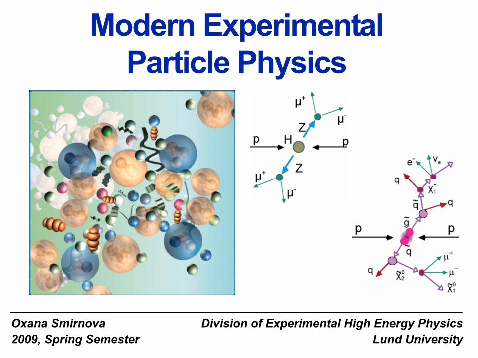
Oxana Smirnova Division of Experimental High Energy Physics2009, Spring Semester Lund University

Modern Experimental Particle Physics

Oxana Smirnova Lund University 2

I. Basic concepts

Figure 1: Object sizes and observation instruments


Main concepts

Particle physics studies elementary “building blocks” of matter and interactions between them.

Matter consists of particles. Matter is built of particles called “fermions”: those that have half-integer spin, e.g. 1/2; obey Fermi-Dirac statistics.

Particles interact via forces.Interaction is an exchange of a force-carrying particle.

Force-carrying particles are called gauge bosons (spin-1).


Forces of nature

Figure 2: Forces and their carriers


Summary table of forces:

Force Acts on/couples to: Carrier Range Strength Stable

systemsInduced reaction

Gravityall particles

Mass/E-p tensor

graviton G

(has not yet been observed)

long∼ Solar system Object falling

Weak forcefermions

hyperchargebosons W+,W-

and Z < m None -decay

Electro-magnetism

charged particles

electric chargephoton γ

long Atoms, molecules

Chemical reactions

Strong forcequarks and

gluons

colour charge

gluons g(8 different) m Hadrons,

nucleiNuclear reactions

F 1 r2⁄∝ 10 39–

10 17– 10 5–β

F 1 r2⁄∝1 137⁄

10 15– 1


The Standard Model

Electromagnetic and weak forces can be described by a single theory ⇒ the “Electroweak Theory” was developed in 1960s (Glashow, Weinberg, Salam).

Theory of strong interactions appeared in 1970s: “Quantum Chromodynamics” (QCD).

The “Standard Model” (SM) combines all the current knowledge.Gravitation is VERY weak at particle scale, and it is not included in the SM. Moreover, quantum theory for gravitation does not exist yet.

Main postulates of SM:

1) Basic constituents of matter are quarks and leptons (spin 1/2)

2) They interact by exchanging gauge bosons (spin 1)

3) Quarks and leptons are subdivided into 3 generations


SM does not explain neither appearance of the mass nor the reason for existence of the 3 generations.

Figure 3: Standard Model: quarks, leptons and bosons


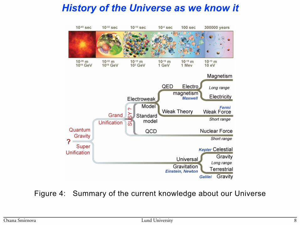
History of the Universe as we know it

Figure 4: Summary of the current knowledge about our Universe


Units and dimensions

Particle energy is measured in electron-volts: 1 eV ≈ 1.602 × 10-19 J (1)

1 eV is energy of an electron upon passing a voltage of 1 Volt.

1 keV = 103 eV; 1 MeV = 106 eV; 1 GeV = 109 eV

The reduced Planck constant and the speed of light: ≡ h / 2π = 6.582 ×10-22 MeV s (2)

c = 2.9979 × 108 m/s (3)

and the “conversion constant” is:c = 197.327 × 10-15 MeV m (4)

For simplicity, natural units are used: = 1 and c = 1 (5)

thus the unit of mass is eV/c2, and the unit of momentum is eV/c

h

h

h


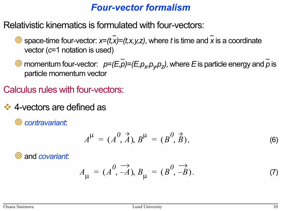
Four-vector formalism

Relativistic kinematics is formulated with four-vectors:space-time four-vector: x=(t,x)=(t,x,y,z), where t is time and x is a coordinate vector (c=1 notation is used)

momentum four-vector: p=(E,p)=(E,px,py,pz), where E is particle energy and p is particle momentum vector

Calculus rules with four-vectors:

4-vectors are defined as contravariant:

, (6)

and covariant:

. (7)

Aμ A0 A,( ) Bμ, B0 B,( )= =

Aμ A0 A–,( ) Bμ, B0 B–,( )= =


Scalar product of two four-vectors is defined as:

. (8)

Scalar products of momentum and space-time four-vectors are thus:

(9)

4-vector product of coordinate and momentum represents particle wavefunction

(10)

4-momentum squared gives particle’s invariant mass

For relativistic particles, we can see that E2=p2+m2 (c=1) (11)

A B⋅ A0B0 A B⋅( )– AμBμ AμBμ= = =

x p⋅ x0p0 x p⋅( )– Et x p⋅( )–= =

p p⋅ p2 p0= p0 p p⋅( )– E2 p2

–= = m2≡


Antiparticles

Particles are described by wavefunctions:

(12)

is the coordinate vector, - momentum vector, E and t are energy and time.

Particles obey the classical Schrödinger equation:

(13)

here (14)

For relativistic particles, E2=p2+m2 (11), and (13) is replaced by the Klein-Gordon equation (15):

⇓

Ψ x t,( ) Nei px Et–( )=

x p

it∂

∂ Ψ x t,( ) HΨ x t,( ) p22m-------Ψ x t,( ) 1

2m-------∇2

Ψ x t,( )–== =

p h2πi--------∇ ∇

i----≡=


(15)

There exist negative energy solutions with E+<0 !

There is a problem with the Klein-Gordon equation: it is second order in derivatives. In 1928, Dirac found the first-order form having the same solutions:

(16)

Here αi and β are 4×4 matrices, and Ψ are four-component wavefunctions: spinors (for particles with spin 1/2).

t2

2

∂

∂– Ψ( ) H2Ψ x t,( ) ∇2Ψ x t,( ) m2

Ψ x t,( )+–==

Ψ∗ x t,( ) N∗ ei p– x E+t+( )

⋅=

i∂Ψ∂t-------- i αi

∂Ψ∂xi-------- βmΨ+

i∑–=

Ψ x t,( )

Ψ1 x t,( )

Ψ2 x t,( )

Ψ3 x t,( )

Ψ4 x t,( )

=


Dirac-Pauli representation of matrices αi and β:

Here I is a 2×2 unit matrix, 0 is a 2×2 matrix of zeros, and σi are 2×2 Pauli matrices:

Also possible is Weyl representation:

αi0 σiσi 0 ⎠

⎟⎟⎞

⎝⎜⎜⎛

= β I 00 I–⎝ ⎠

⎜ ⎟⎛ ⎞

=

σ10 11 0⎝ ⎠

⎜ ⎟⎛ ⎞

= σ20 i–i 0⎝ ⎠

⎜ ⎟⎛ ⎞

= σ31 00 1–⎝ ⎠

⎜ ⎟⎛ ⎞

=

αiσi– 0

0 σi ⎠⎟⎟⎞

⎝⎜⎜⎛

= β 0 II 0⎝ ⎠

⎜ ⎟⎛ ⎞

=


Dirac’s picture of vacuum

The “hole” created by appearance of an electron with “normal” energy is interpreted as the presence of electron’s antiparticle with the opposite charge.

Every charged particle must have an antiparticle of the same mass and opposite charge, to solve the mystery of “negative” energy.

Figure 5: Fermions in Dirac’s representation


Discovery of the positron1933, C.D.Andersson, Univ. of California (Berkeley) observed with the Wilson cloud chamber 15 tracks in cosmic rays:

Figure 6: Photo of the track in the Wilson chamber

positrontrack

lead plate


Feynman diagrams

In 1940s, R.Feynman developed a diagram technique for representing processes in particle physics.

Main assumptions and requirements:Time runs from left to right

Arrow directed towards the right indicates a particle, and otherwise - antiparticle

At every vertex, momentum, angular momentum and charge are conserved (but not necessarily energy)

Particles are shown by solid lines, gauge bosons - by helices or dashed lines

Figure 7: A Feynman diagram example: e+e- -> γ


A virtual process does not require energy conservation

a) e- → e- + γ b) γ + e- → e-

c) e+ → e+ + γ d) γ + e+ → e+

e) annihilation e+ + e- → γ f) pair production γ → e+ + e-

g) vacuum → e+ + e- + γ h) e+ + e- + γ → vacuum

Figure 8: Feynman diagrams for VIRTUAL processes involving e+, e- and γ


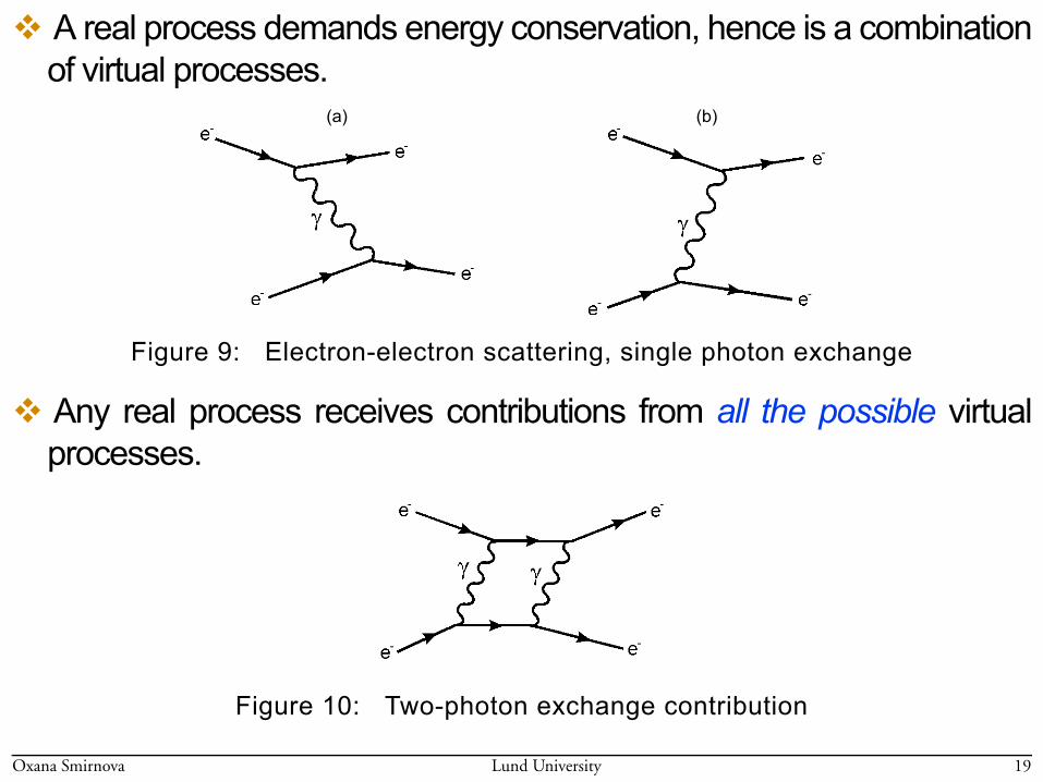
A real process demands energy conservation, hence is a combination of virtual processes.

Any real process receives contributions from all the possible virtual processes.

(a) (b)

Figure 9: Electron-electron scattering, single photon exchange

Figure 10: Two-photon exchange contribution


Probability P(e-e- → e-e-) = |M(1 γ exchange) + M(2 γ exchange) + M(3 γ exchange) +... |2 (M stands for contribution, “Matrix element”)

Number of vertices in a diagram is called its order. Each vertex has an associated probability proportional to a coupling constant, usually denoted as “α”. In discussed processes this constant is

(17)

Matrix element for a two-vertex process is proportional to , where each vertex has a factor . Probability for a process is P=|M|2=α2

For the real processes, a diagram of order n gives a contribution to probability of order αn.

Provided sufficiently small α, high order contributions are smaller and smaller and the result is convergent: P(real) = |M(α)+M(α2)+M(α3)...|2

Often lowest order calculation is precise enough.

αeme2

4πε0------------ 1

137--------- 1«≈=

M α α⋅=α


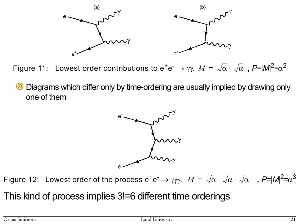
Diagrams which differ only by time-ordering are usually implied by drawing only one of them

This kind of process implies 3!=6 different time orderings

(a) (b)

Figure 11: Lowest order contributions to e+e- → γγ. , P=|M|2=α2

Figure 12: Lowest order of the process e+e- → γγγ. , P=|M|2=α3

M α α⋅=

M α α α⋅ ⋅=


Knowing order of diagrams is sufficient to estimate the ratio of appearance rates of processes:

This ratio can be measured experimentally; it appears to be R= 0.9×10-3, which is smaller than αem, being only a first order prediction.

For nuclei, the coupling is proportional to Z2α, hence the rate of this process is of order Z2α3

Figure 13: Diagrams that are not related by time ordering

R Rate e+e- γγγ→( )

Rate e+e- γγ→( )-----------------------------------------------≡ O α3( )

O α2( )---------------- O= α( )=


Exchange of a massive boson

In the rest frame of particle A:

where , , ,

From this one can estimate the maximum distance over which X can propagate before being absorbed: , and this

energy violation can exist only for a period of time Δt≈ /ΔE(Heisenberg’s uncertainty relation), hence the range of the interaction is r ≈ R ≡( / MX )c = Δt c

Figure 14: Exchange of a massive particle X

A E0 p0,( ) A EA p,( ) X Ex p–,( )+→

E0 MA= p0 0 0 0, ,( )= EA p2 MA2+= EX p2 MX

2+=

ΔE EX EA MA MX≥–+=

h_

h_


For a massless exchanged particle, the interaction has an infinite range (e.g., electromagnetic)

In case of a very heavy exchanged particle (e.g., a W boson in weak interaction), the interaction can be approximated by a zero-range, or point interaction:

E.g., for a W boson: RW = /MW = /(80.4 GeV/c2) ≈ 2 × 10-18 m

Figure 15: Point interaction as a result of Mx → ∞

h_

h_


Yukawa potential (1935)

Considering particle X as an electrostatic spherically symmetric potential V(r), the Klein-Gordon equation (15) for it will look like

(18)

(In 3D polar coordinates system, , ).

Integration of (18) gives the solution of

(19)

Here g is an integration constant, and it is interpreted as the coupling strength for particle X to the particles A and B.

V r( )∇2 1r2----- ∂

∂r----- r2∂V

∂r------⎝ ⎠

⎛ ⎞ MX2 V r( )==

t2

2

∂∂ V r( ) 0( )= ∇2V r( ) 1

r2----- ∂

∂r----- r2

r∂∂ V r( )⎝ ⎠

⎛ ⎞=

V r( ) g2

4πr---------e r R⁄––=


In Yukawa theory, g is analogous to the electric charge in QED, and the analogue of αem is

αX characterizes the strength of the interaction at distances r ≤ R.

Consider a particle being scattered by the potential (19), thus receiving a

momentum transfer

Potential (19) has the corresponding amplitude, which is its Fourier-transform (like in optics):

(20)

αXg2

4π------=

q

f q( ) V x( )eiqxd3x∫=


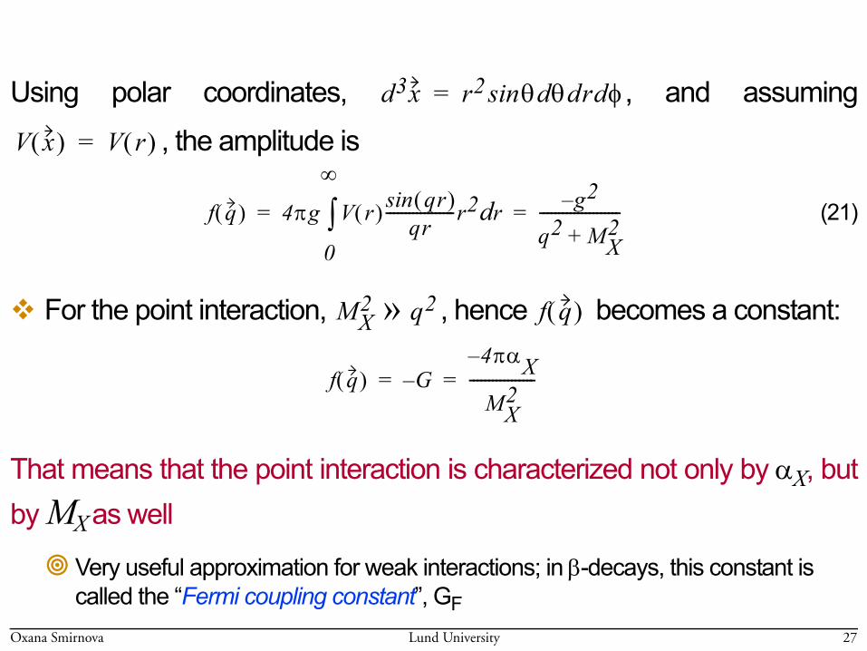
Using polar coordinates, , and assuming

, the amplitude is

(21)

For the point interaction, , hence becomes a constant:

That means that the point interaction is characterized not only by αX, but by MX as well

Very useful approximation for weak interactions; in β-decays, this constant is called the “Fermi coupling constant”, GF

d3x r2 θdθdrdφsin=

V x( ) V r( )=

f q( ) 4πg V r( ) qr( )sinqr

------------------r2 rd0

∞

∫g– 2

q2 MX2+

---------------------= =

MX2 q2» f q( )

f q( ) G–4– παXMX

2-----------------= =

Modern Experimental Particle Physics - Lunds … · Oxana Smirnova Lund University 3 Main concepts...

Documents

Transcript of Modern Experimental Particle Physics - Lunds … · Oxana Smirnova Lund University 3 Main concepts...