Modern Approach for Designing and Solving Interval ... · programming model (IELFPM) are obtained...
16
795 Available at http://pvamu.edu/aam Appl. Appl. Math. ISSN: 1932-9466 Vol. 9, Issue 2 (December 2014), pp. 795-810 Applications and Applied Mathematics: An International Journal (AAM) Modern Approach for Designing and Solving Interval Estimated Linear Fractional Programming Models S. Ananthalakshmi Department of Statistics Manonmaniam Sundaranar University Tirunelveli 627 012 Tamilnadu, India [email protected] C. Vijayalakshmi and V. Ganesan Department of Mathematics VIT University, Chennai Campus Chennai-600 127 Tamilnadu, India [email protected] Received: March 23, 2013; Accepted: June 26, 2013 Abstract Optimization methods have been widely applied in statistics. In mathematical programming, the coefficients of the models are always categorized as deterministic values. However uncertainty always exists in realistic problems. Therefore, interval-estimated optimization models may provide an alternative choice for considering the uncertainty into the optimization models. In this aspect, this paper concentrates, the lower and upper values of interval estimated linear fractional programming model (IELFPM) are obtained by using generalized confidence interval estimation method. An IELFPM is a LFP with interval form of the coefficients in the objective function and all requirements. The solution of the IELFPM is also analyzed. Keywords: Interval estimated linear fractional programming model (IELFPM); linear fractional programming (LFP); interval valued function (IVF); optimum solution; confidence interval MSC 2010 No.: 90C05, 90C32, 90C30, 65K99
Transcript of Modern Approach for Designing and Solving Interval ... · programming model (IELFPM) are obtained...

795
Available at
http://pvamu.edu/aam Appl. Appl. Math.
ISSN: 1932-9466
Vol. 9, Issue 2 (December 2014), pp. 795-810
Applications and Applied
Mathematics:
An International Journal
(AAM)
Modern Approach for Designing and Solving Interval
Estimated Linear Fractional Programming Models
S. Ananthalakshmi Department of Statistics
Manonmaniam Sundaranar University
Tirunelveli 627 012
Tamilnadu, India
C. Vijayalakshmi and V. Ganesan Department of Mathematics
VIT University, Chennai Campus
Chennai-600 127
Tamilnadu, India
Received: March 23, 2013; Accepted: June 26, 2013
Abstract
Optimization methods have been widely applied in statistics. In mathematical programming, the
coefficients of the models are always categorized as deterministic values. However uncertainty
always exists in realistic problems. Therefore, interval-estimated optimization models may
provide an alternative choice for considering the uncertainty into the optimization models. In this
aspect, this paper concentrates, the lower and upper values of interval estimated linear fractional
programming model (IELFPM) are obtained by using generalized confidence interval estimation
method. An IELFPM is a LFP with interval form of the coefficients in the objective function and
all requirements. The solution of the IELFPM is also analyzed.
Keywords: Interval estimated linear fractional programming model (IELFPM); linear
fractional programming (LFP); interval valued function (IVF); optimum solution;
confidence interval
MSC 2010 No.: 90C05, 90C32, 90C30, 65K99
796 S. Ananthalakshmi et al.
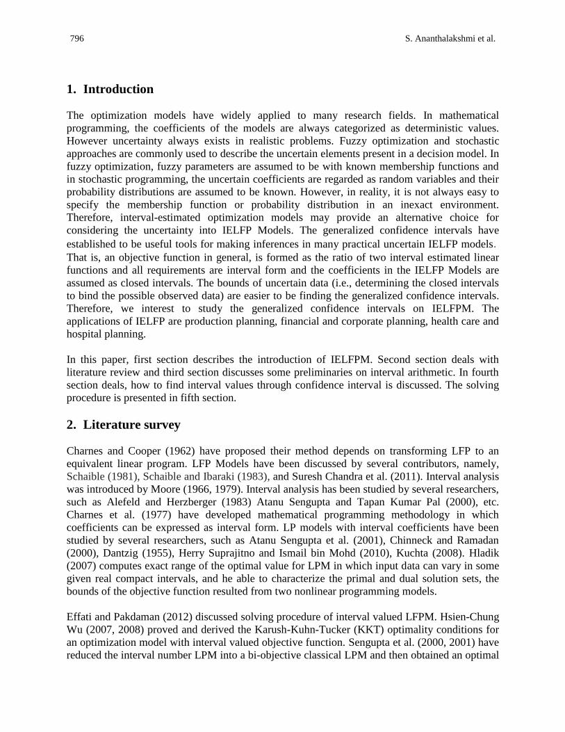
1. Introduction
The optimization models have widely applied to many research fields. In mathematical
programming, the coefficients of the models are always categorized as deterministic values.
However uncertainty always exists in realistic problems. Fuzzy optimization and stochastic
approaches are commonly used to describe the uncertain elements present in a decision model. In
fuzzy optimization, fuzzy parameters are assumed to be with known membership functions and
in stochastic programming, the uncertain coefficients are regarded as random variables and their
probability distributions are assumed to be known. However, in reality, it is not always easy to
specify the membership function or probability distribution in an inexact environment.
Therefore, interval-estimated optimization models may provide an alternative choice for
considering the uncertainty into IELFP Models. The generalized confidence intervals have
established to be useful tools for making inferences in many practical uncertain IELFP models. That is, an objective function in general, is formed as the ratio of two interval estimated linear
functions and all requirements are interval form and the coefficients in the IELFP Models are
assumed as closed intervals. The bounds of uncertain data (i.e., determining the closed intervals
to bind the possible observed data) are easier to be finding the generalized confidence intervals.
Therefore, we interest to study the generalized confidence intervals on IELFPM. The
applications of IELFP are production planning, financial and corporate planning, health care and
hospital planning.
In this paper, first section describes the introduction of IELFPM. Second section deals with
literature review and third section discusses some preliminaries on interval arithmetic. In fourth
section deals, how to find interval values through confidence interval is discussed. The solving
procedure is presented in fifth section.
2. Literature survey
Charnes and Cooper (1962) have proposed their method depends on transforming LFP to an
equivalent linear program. LFP Models have been discussed by several contributors, namely,
Schaible (1981), Schaible and Ibaraki (1983), and Suresh Chandra et al. (2011). Interval analysis
was introduced by Moore (1966, 1979). Interval analysis has been studied by several researchers,
such as Alefeld and Herzberger (1983) Atanu Sengupta and Tapan Kumar Pal (2000), etc.
Charnes et al. (1977) have developed mathematical programming methodology in which
coefficients can be expressed as interval form. LP models with interval coefficients have been
studied by several researchers, such as Atanu Sengupta et al. (2001), Chinneck and Ramadan
(2000), Dantzig (1955), Herry Suprajitno and Ismail bin Mohd (2010), Kuchta (2008). Hladik
(2007) computes exact range of the optimal value for LPM in which input data can vary in some
given real compact intervals, and he able to characterize the primal and dual solution sets, the
bounds of the objective function resulted from two nonlinear programming models.
Effati and Pakdaman (2012) discussed solving procedure of interval valued LFPM. Hsien-Chung
Wu (2007, 2008) proved and derived the Karush-Kuhn-Tucker (KKT) optimality conditions for
an optimization model with interval valued objective function. Sengupta et al. (2000, 2001) have
reduced the interval number LPM into a bi-objective classical LPM and then obtained an optimal

AAM: Intern. J., Vol. 9, Issue 2 (December 2014) 797
solution. Suprajitno and Mohd (2008) and Suprajitno et al. (2009) presented some interval linear
programming models, where the coefficients and variables are in the form of intervals.
Krishnamoorthy and Mathew (2004) discussed on one sided tolerance limits in balanced and
unbalanced one-way random effects ANOVA model. Weerahandi (2004) has introduced the
concept of a generalized pivotal quantity (GPQ) for a scalar parameter µ and using that
parameter, one can construct an interval estimator for µ in situations where standard pivotal
quantity based approaches may not be applicable. He referred to such intervals as generalized
confidence intervals (GCI).
3. Preliminaries
This section is to present some notations, which are useful in our further consideration.
Let us denote by I the class of all closed and bounded intervals in R. If a and b are closed and
bounded intervals, we also adopt the notation aaa , and bbb , , where ba, and ba,
mean the lower and upper bounds of a and b . Let aaa , and bbb , be in I. Then,
by definition,
(i) , .a b a b a b I
(ii) , .a b a b a b I
(iii) , .a a a I
(iv) , , if 0,
,, , if 0,
x a xa xx a a
xa xa x
where x is a real number.
(v) An interval a is said to be positive, if 0a and negative, if 0a .
(vi) If aaa , and bbb , are bounded and real intervals, we define the
multiplication of two intervals as follows:
min , , , , max , , ,a b ab ab ab ab ab ab ab ab
,
1) If 0 and 0a a b b , then we have
ababba , . (3.1)

798 S. Ananthalakshmi et al.
2) If bbaa 0and0 , then we have
abbaba , . (3.2)
(vii) There are several approaches to define interval division. We define the quotient of two
intervals as follows:
Let aaa , and also bbb , be two nonempty bounded real intervals. Then, if
0 ],[ bb , we have
bbaaba
1,
1],[][][ . (3.3)
(viii) Power of interval for n Z is given as:
When n is positive and odd or a is positive, then nnnaaa , .
When n is positive and even, then
, , if 0,
, , if 0,
[0,max{ ) , ( ) }], otherwise.
n n
nn n
n n
a a a
a a a a
a a
When n is negative and odd or even, then
n
n
aa
][
1 .
(ix) For an interval a such that 0a , define the square root of a denoted by ][a as:
][a = { abab : }.
(x) Mid-point of an interval a is defined as aaam 2
1)][( .
(xi) Width of an interval a is defined as aaaw )][( .
(xii) Half-width of an interval a is defined as )(2
1)][( aaahw .
AAM: Intern. J., Vol. 9, Issue 2 (December 2014) 799
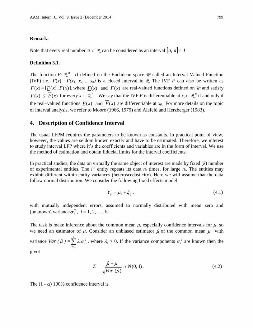
Remark:
Note that every real number a R can be considered as an interval Iaa , .
Definition 3.1.
The function F: R n I defined on the Euclidean space Rn called an Interval Valued Function
(IVF) i.e., F(x) =F(x1, x2, …, xn) is a closed interval in R. The IVF F can also be written as
( ) [ ( ), ( ) ],F x F x F x where )(and)( xFxF are real-valued functions defined on Rn and satisfy
)()( xFxF for every x R n. We say that the IVF F is differentiable at x0 R
n if and only if
the real–valued functions )(and)( xFxF are differentiable at x0. For more details on the topic
of interval analysis, we refer to Moore (1966, 1979) and Alefeld and Herzberger (1983).
4. Description of Confidence Interval
The usual LFPM requires the parameters to be known as constants. In practical point of view,
however, the values are seldom known exactly and have to be estimated. Therefore, we interest
to study interval LFP where it’s the coefficients and variables are in the form of interval. We use
the method of estimation and obtain fiducial limits for the interval coefficients.
In practical studies, the data on virtually the same object of interest are made by fixed (k) number
of experimental entities. The ith
entity repeats its data ni times, for large ni. The entities may
exhibit different within entity variances (heteroscedasticity). Here we will assume that the data
follow normal distribution. We consider the following fixed effects model
ijiijY , (4.1)
with mutually independent errors, assumed to normally distributed with mean zero and
(unknown) variance 2
i , i = 1, 2, …, k.
The task is make inference about the common mean , especially confidence intervals for , so
we need an estimator of . Consider an unbiased estimator ̂ of the common mean with
variance Var ( ̂ ) =
k
i
ii
1
2 , where i > 0. If the variance components 2
i are known then the
pivot
)1,0()ˆ(
ˆN
VarZ
. (4.2)
The (1 - ) 100% confidence interval is

800 S. Ananthalakshmi et al.
)ˆ()2/1(ˆ)ˆ()2/1(ˆ VarVar , (4.3)
where (.) is quantile function of normal distribution. If the variance components 2
i are
unknown then we find the exact distribution of Z.
So we want to compare some approximate confidence intervals for common mean derived from
the simple t-statistic, the t-statistic with Satterthwaite’s degrees of freedom, the t-statistic derived
from Kenward- Roger method and by Welch’s quantile approximation.
Interval derived from simple t-statistic
The simple t-statistic T is given by
)( n
n
YVar
YT
, (4.4)
where
NSYVar n
2
)( ,
.)1()(,)()1(
,,,
1
212
1
2.
12
1
.1
1 1
1.
k
i
ii
n
j
iijii
k
i
iin
k
i
n
j
ijiii
SnkNSYYnS
YnNYYnYnN
i
i
This statistic was derived under the assumption of the variance homogeneity and has a t-
distribution with N - k degrees of freedom.
The (1 - ) 100% confidence interval is
)()( )2/1()2/1( nkNnnkNn YVartYYVartY , (4.5)
where tdf (.) is quantile function of Student’s t-distribution with df degrees of freedom.
Interval derived from t-statistic with Satterthwaite’s degrees of freedom
The t-test, Ts, is given by
)( n
n
S
YVar
YT
, (4.6)
where
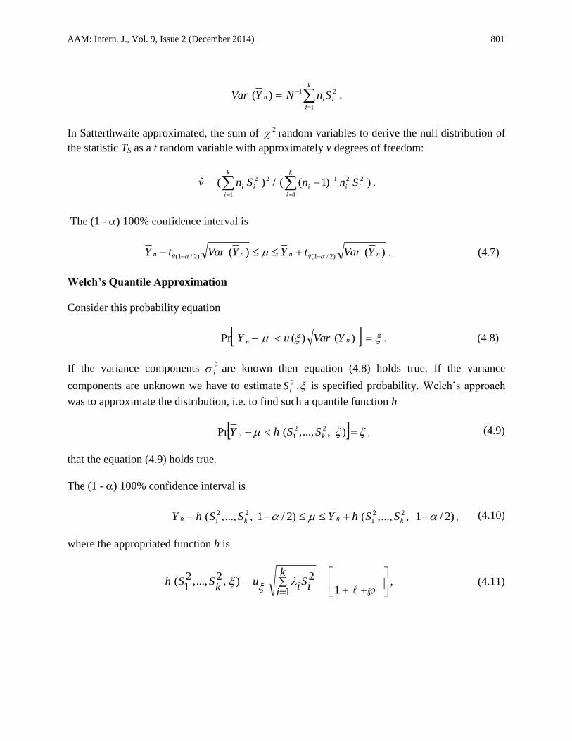
AAM: Intern. J., Vol. 9, Issue 2 (December 2014) 801
k
i
iin SnNYVar1
21)( .
In Satterthwaite approximated, the sum of 2 random variables to derive the null distribution of
the statistic TS as a t random variable with approximately v degrees of freedom:
))1((/)(ˆ1
2212
1
2
k
i
iii
k
i
ii SnnSnv .
The (1 - ) 100% confidence interval is
)()( )2/1(ˆ)2/1(ˆ nvnnvn YVartYYVartY . (4.7)
Welch’s Quantile Approximation
Consider this probability equation
)()(Pr nn YVaruY . (4.8)
If the variance components 2
i are known then equation (4.8) holds true. If the variance
components are unknown we have to estimate 2
iS . is specified probability. Welch’s approach
was to approximate the distribution, i.e. to find such a quantile function h
),...,,(Pr 22
1 kn SShY , (4.9)
that the equation (4.9) holds true.
The (1 - ) 100% confidence interval is
)2/1,...,,()2/1,...,,( 22
1
22
1 knkn SShYSShY , (4.10)
where the appropriated function h is
1
2
1),2...,,2
1( iS
k
iiu
kSSh
, (4.11)

802 S. Ananthalakshmi et al.
,
32
)/(93215
3
/53
,
2
/1
4
/1
4
1
2
1
242442
3
1
2
1
26342
2
1
2
1
2422
2
1
2
1
422
k
iii
k
iiii
k
iii
k
iiii
k
iii
k
iiii
k
iii
k
iiii
S
fSuuu
S
fSuu
S
fSu
S
fSu
fi = ni - 1, 2N
ni
i , for i = 1, 2, …, k.
Interval Derived by Kenward Roger Method
Kenward and Roger derived the method to estimate the variance of the generalized least square
estimator (GLSE) and derived a test statistic about expected values.
)( ˆ
ˆ
YVar
YTKR
, (4.12)
where
,ˆ2
1
1ˆ)ˆ(
k
iiYVar
12ˆ ˆ ˆˆ/ , ,
1 1
k kn S Y Yii i i i i
i i
and ̂ is penalty derived from Kenward and Roger method. The statistic TKR has a t-distribution
with approximately m̂ degrees of freedom, where degrees of freedom m̂ are derived by
Satterthwaite’s method.
The (1 - ) 100% confidence interval is
)()( ˆ)2/1(ˆˆˆ)2/1(ˆ YVartYYVartY mm . (4.13)
AAM: Intern. J., Vol. 9, Issue 2 (December 2014) 803
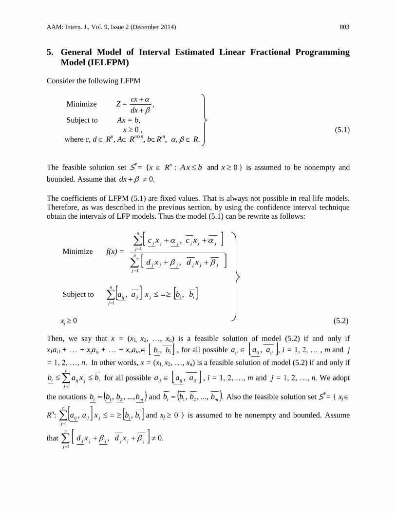
5. General Model of Interval Estimated Linear Fractional Programming
Model (IELFPM)
Consider the following LFPM
Minimize Z =
dx
cx,
Subject to Ax = b,
x 0 , (5.1)
where c, d Rn, A R
mxn, bR
m, , R.
The feasible solution set S*= {x R
n : 0and xbxA } is assumed to be nonempty and
bounded. Assume that dx 0.
The coefficients of LFPM (5.1) are fixed values. That is always not possible in real life models.
Therefore, as was described in the previous section, by using the confidence interval technique
obtain the intervals of LFP models. Thus the model (5.1) can be rewrite as follows:
Minimize f(x) =
n
j
jjjjjj
n
j
jjjjjj
xdxd
xcxc
1
1
,
,
Subject to iij
n
j
ijij bbxaa ,,1
xj 0 (5.2)
Then, we say that x = (x1, x2, …, xn) is a feasible solution of model (5.2) if and only if
x1ai1 + … + xjaij + … + xnain ii bb , , for all possible ijijij aaa , , i = 1, 2, … , m and j
= 1, 2, …, n. In other words, x = (x1, x2, …, xn) is a feasible solution of model (5.2) if and only if
i
n
ij
jiji bxab
for all possible ijijij aaa , , i = 1, 2, …, m and j = 1, 2, …, n. We adopt
the notations mi bbbb ...,,, 21 and mi bbbb ...,,, 21 . Also the feasible solution set S*= { xj
Rn: iij
n
j
ijij bbxaa ,,1
and xj 0 } is assumed to be nonempty and bounded. Assume
that
n
j
jjjjjj xdxd1
, 0.

804 S. Ananthalakshmi et al.
Let
p(x) =
n
j
jjjjjj xcxc1
, , (5.3)
q(x) =
n
j
jjjjjj xdxd1
, . (5.4)
From (5.3) and (5.4) we consider
)(xp
n
j
jjj xc1
)( , )(xp )(1
n
j
jjj xc ,
)(xq =
n
j
jjj xd1
)( , )(xq =
n
j
jjj xd1
)( .
We suppose that 0 q(x) for each feasible solution x, so we should have
0 < )(xq )(xq or )(xq )(xq < 0. (5.5)
Using preliminaries (vii) and equation (3.3) the objective function of IVLFP of the model (5.2)
can be rewrite into the following form
f(x)=
n
j jjjjjj
jjjjjjxdxd
xcxc1
1,
1,
. (5.6)
Now we can consider two possible cases:
Case (1) When 0 < )(xq )(xq , we have two possibilities
i) If 0 )(xp )(xp , using preliminaries (vi) and equation (3.1) we have
f(x) =
n
j jjj
jjj
jjj
jjj
xd
xc
xd
xc
1
,
. (5.7)
ii) If )(xp < )(xp < 0, using preliminaries (vi) and equation (3.2) we have
AAM: Intern. J., Vol. 9, Issue 2 (December 2014) 805
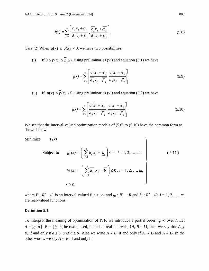
f(x) =
n
j jjj
jjj
jjj
jjj
xd
xc
xd
xc
1
,
. (5.8)
Case (2) When )(xq )(xq < 0, we have two possibilities:
(i) If 0 )(xp )(xp , using preliminaries (vi) and equation (3.1) we have
f(x) =
n
j jjj
jjj
jjj
jjj
xd
xc
xd
xc
1
,
. (5.9)
(ii) If )(xp < )(xp < 0, using preliminaries (vi) and equation (3.2) we have
f(x) =
n
j jjj
jjj
jjj
jjj
xd
xc
xd
xc
1
,
. (5.10)
We see that the interval-valued optimization models of (5.6) to (5.10) have the common form as
shown below:
Minimize F(x)
Subject to gi (x) =
ij
n
j
ij bxa1
0, i = 1, 2, …, m, ( 5.11 )
hi (x ) =
ij
n
j
ij bxa1
0 , i = 1, 2, …, m,
xi 0.
where F : Rn →I is an interval-valued function, and gi : R
n →R and hi : R
n →R, i = 1, 2, …, m,
are real-valued functions.
Definition 5.1.
To interpret the meaning of optimization of IVF, we introduce a partial ordering over I. Let
A = ],[ aa , B = ],[ bb be two closed, bounded, real intervals, IBA , , then we say that A
B, if and only if baandba . Also we write A B, if and only if A B and A B. In the
other words, we say A B, if and only if
806 S. Ananthalakshmi et al.
.bababa
oror
bababa
(5.12)
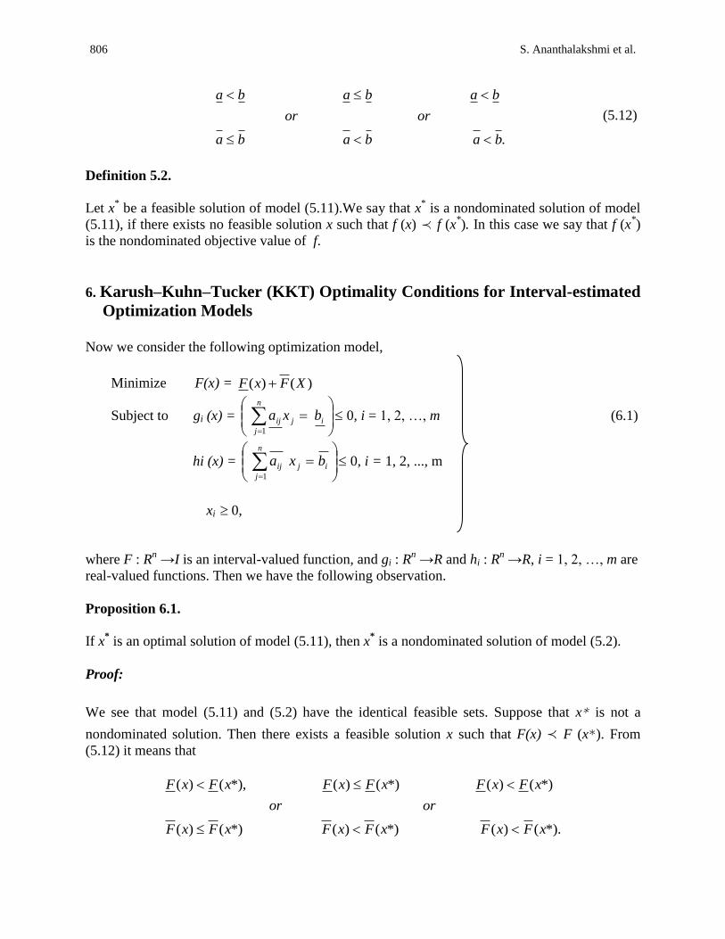
Definition 5.2.
Let x* be a feasible solution of model (5.11).We say that x
* is a nondominated solution of model
(5.11), if there exists no feasible solution x such that f (x) f (x*). In this case we say that f (x
*)
is the nondominated objective value of f.
6. Karush–Kuhn–Tucker (KKT) Optimality Conditions for Interval-estimated
Optimization Models
Now we consider the following optimization model,
Minimize F(x) = )()( XFxF
Subject to gi (x) =
ij
n
j
ij bxa1
0, i = 1, 2, …, m (6.1)
hi (x) =
ij
n
j
ij bxa1
0, i = 1, 2, ..., m
xi 0,
where F : Rn →I is an interval-valued function, and gi : R
n →R and hi : R
n →R, i = 1, 2, …, m are
real-valued functions. Then we have the following observation.
Proposition 6.1.
If x* is an optimal solution of model (5.11), then x
* is a nondominated solution of model (5.2).
Proof:
We see that model (5.11) and (5.2) have the identical feasible sets. Suppose that x∗ is not a
nondominated solution. Then there exists a feasible solution x such that F(x) ≺ F (x∗). From
(5.12) it means that
*).()(*)()(*)()(
*)()(*)()(*),()(
xFxFxFxFxFxF
oror
xFxFxFxFxFxF
AAM: Intern. J., Vol. 9, Issue 2 (December 2014) 807
It also shows that F (x) < F (x∗), which contradicts the fact that x∗, is an optimal solution of
model (5.11). We complete the proof.
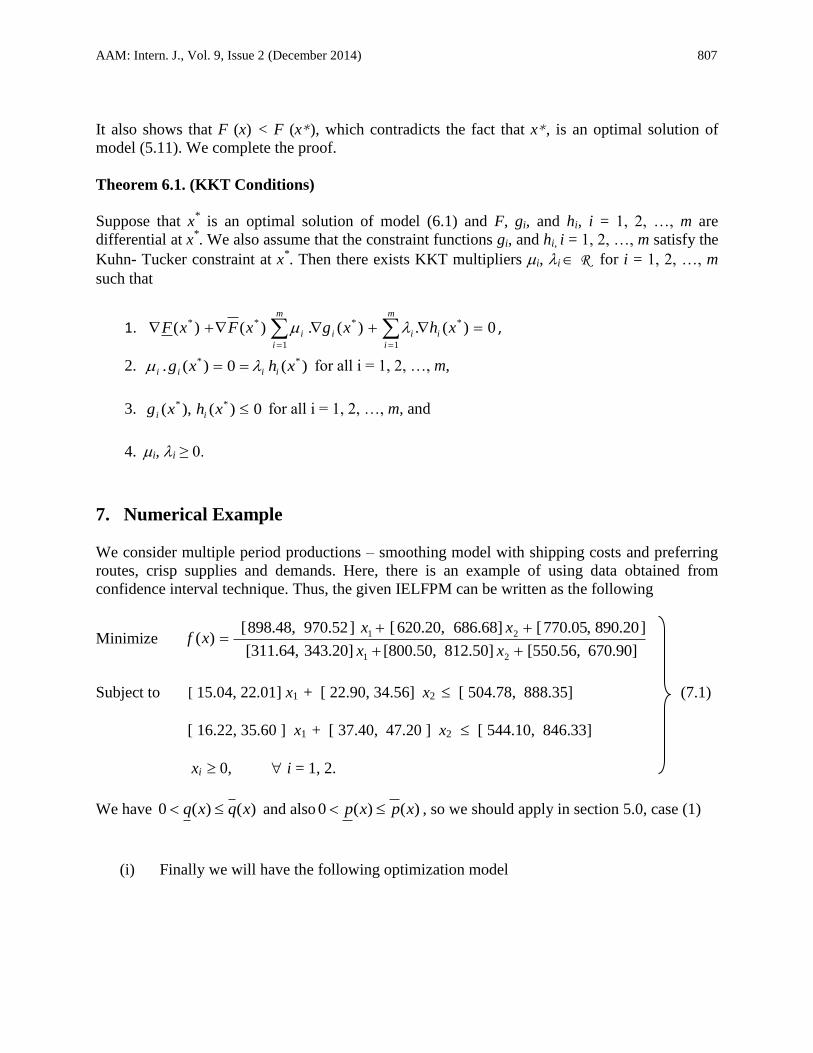
Theorem 6.1. (KKT Conditions)
Suppose that x* is an optimal solution of model (6.1) and F, gi, and hi, i = 1, 2, …, m are
differential at x*. We also assume that the constraint functions gi, and hi, i = 1, 2, …, m satisfy the
Kuhn- Tucker constraint at x*. Then there exists KKT multipliers i, i R for i = 1, 2, …, m
such that
1. 0)(.)(.)()( *
1
*
1
**
xhxgxFxF i
m
i
ii
m
i
i ,
2. )(0)(. ** xhxg iiii for all i = 1, 2, …, m,
3. 0)(),( ** xhxg ii for all i = 1, 2, …, m, and
4. i, i ≥ 0.
7. Numerical Example
We consider multiple period productions – smoothing model with shipping costs and preferring
routes, crisp supplies and demands. Here, there is an example of using data obtained from
confidence interval technique. Thus, the given IELFPM can be written as the following
Minimize 670.90][550.56, 812.50] [800.50, 343.20] [311.64,
]20.890,05.770[ 686.68] 620.20,[ ]970.52 898.48,[ )(
21
21
xx
xxxf
Subject to [ 15.04, 22.01] x1 + [ 22.90, 34.56] x2 [ 504.78, 888.35] (7.1)
[ 16.22, 35.60 ] x1 + [ 37.40, 47.20 ] x2 [ 544.10, 846.33]
xi 0, i = 1, 2.
We have )()(0 xqxq and also )()(0 xpxp , so we should apply in section 5.0, case (1)
(i) Finally we will have the following optimization model

808 S. Ananthalakshmi et al.
Minimize
90.67050.81220.343
20.89068.68652.970,
56.55050.80064.311
05.77020.62048.898)(
21
21
21
21
xx
xx
xx
xxxf
Subject to g1( 1x , 2x ) = 15.04 1x + 22.90 2x = 504.78
h1( 1x , 2x ) = 22.01 1x + 34.56 2x = 888.35
g2( 1x , 2x ) = 16.22 1x + 37.40 2x = 544.10
(7.2)
h2( 1x , 2x ) = 35.60 1x + 47.20 2x = 846.33
1x , 2x 0.
Now to obtain a nondominated solution for (7.2), we use proposition (6.1) and solve the
following optimization model
Minimize
90.6705.81220.343
20.89068.68652.970
56.55050.80064.311
05.77020.62048.898)(
21
21
21
21
xx
xx
xx
xxxf
Subject to 15.04 1x + 22.90 2x = 504.78
22.01 1x + 34.56 2x = 888.35
16.22 1x + 37.40 2x = 544.10
(7.3)
35.60 1x + 47.20 2x = 846.33
1x , 2x 0.
By using Excel Solver, the optimal solution is *
1x 10.55255, *
2x = 9.971596 with optimal value
(x*) = 2.840901
8. Conclusion
In this paper, first we introduce a LFPM with interval valued parameters. Then we have
suggested using confidence intervals for estimating interval values to IELFPM. In practical point
of view, confidence intervals based on t- statistic and Welch’s method has very good reporting
properties for almost all cases. The method based on Satterthwaite’s degrees of freedom has
good reporting properties whenever the number of observations in one experimental unit is

AAM: Intern. J., Vol. 9, Issue 2 (December 2014) 809
sufficiently large or number of experimental units is increasing. The method based on Kenward
and Roger does not have good properties for this model with small number of observations in
one experimental unit. By using Karush–Kuhn–Tucker optimality conditions, it is proved that we
can convert the model of the IELFPM to the nonlinear fractional programming model and
obtained an optimal solution. The study of very complicated system can be done with the help of
this model and can be adapted to adjust the variation in the uncertain environments of real
situations. Work is in progress to apply and check the approach for solving optimization problem
under interval data environment.
REFERENCES
Alefeld, G. and Herzberger, J. (1983). Introduction to interval computations, Academic Press,
New York.
Atanu Sengupta, and Tapan Kumar Pal (2000). Theory and Methodology: On comparing interval
numbers, European Journal of Operational Research, 27: 28 - 43.
Atanu Sengupta, Tapan Kumar Pal and Debjani Chakraborty (2001). Interpretation of inequality
constraints involving interval coefficients and a solution to interval linear programming-
Fuzzy Sets and Systems, European Journal of Operational Research, 119:129-138.
Charnes, A. and Cooper, W. W. (1962). Naval Research Log. Quart., 9:181-186.
Charnes, A., Granot, F. and Phillips, E. (1977). An algorithm for solving interval linear
programming problems, Operations Research 25: 688-695.
Chinneck, J.W. and Ramadan, K. (2000). Linear programming with interval coefficients, JORS,
51: 209-220.
Dantzig, G. B. (1955). Linear programming under uncertainty, Management Science, 1: 197-206.
Herry Suprajitno and Ismail bin Mohd (2010). Linear Programming with Interval Arithmetic, Int.
J. Contemp. Math. Sciences, 5(7): 323 – 332.
Hladik M. (2007). Optimal value range in interval linear programming, Faculty of Mathematics
and Physics, Charles University, Prague.
Krishnamoorthy, K. and Mathew, T. (2004). One-sided tolerance limits in balanced and
unbalanced one-way random models based on generalized confidence limits, Technometrics,
46: 44–52.
Kuchta, D. (2008). A modification of a solution concept of the linear programming problem with
interval coefficients in the constraints, CEJOR, 16: 307-316.
Moore, R. E. (1966). Interval analysis. Englewood Cliffs, NJ: Prentice-Hall.
Moore, R. E. (1979). Method and Application of Interval Analysis, Philadelphia, SIAM.
Schaible, S. (1981). Fractional programming: applications and algorithms, European Journal of
Operational Research, 7(2): 111-120.
Schaible, S. and Ibaraki, T. (1983). Fractional programming, European Journal of Operational
Research, 12(3): 325-338.
Sohrab Effati and Morteza Pakdaman (2012). Solving the Interval-Valued Linear Fractional
Programming Problem, American Journal of Computational Mathematics, 2:51-55
Suprajitno H. and Mohd I.B. (2008). Interval Linear Programming, presented in ICoMS-3,
Bogor, Indonesia.
810 S. Ananthalakshmi et al.
Suprajitno H., Mohd I.B., Mamat M. and Ismail F. (2009). Linear Programming with Interval
Variables, presented in 2nd ICOWOBAS, Johor Bahru, Malaysia.
Suresh Chandra, Jayadeva and Aparna Mehra (2011). Numerical Optimization with
Applications, Narosa Publishing House, New Delhi, 442-475.
Weerahandi S. (2004). Generalized Inference in Repeated Measures, New York Wiley.
Wu H.-C. (2007). The Karush-Kuhn-Tucker Optimality Conditions in an Optimization Problem
with Interval- valued Objective Function, European Journal of Operational Research,
176(1): 46-59.
Wu H.-C. (2008). On Interval-Valued Nonlinear Programming Problems, Journal of
Mathematical Analysis and Applications, 338(1): 299-316.
Authors’ Bios
Dr. S. Ananthalakshmi is currently working as Assistant Professor in Department of Mathematics, Annai Hajira
Women’s, College, Malapalayam, Tirunelveli Tamilnadu (India). She is a Visiting Professor in Department of
Statistics, Manonmaniam Sundaranar University, Tirunelveli, Tamil Nadu Her research interests concern applied
mathematical methods for advanced linear programming model, risk analysis, uncertainty analysis, inventory
management, sensitivity analysis and decision analysis. She is a life member of the Indian Society for Probability
and Statistics.
Dr. C. Vijayalakshmi is currently working as Associate Professor in SAS,Mathematics Division,VIT University,
Chennai, Tamil Nadu. She has more than 15 years of teaching experience at Graduate and Post Graduate level. She
has published more than Twenty research papers in International and National Journals and authored three books for
Engineering colleges, Anna University. She has received Bharat Jyothi Award for outstanding services,
achievements and contributions, Best Teachers award for academic excellence. Her area of specialization is
Stochastic Processes and their applications. Her other research interests include Optimization Techniques, Data
mining and Bio-Informatics.
Dr. V. Ganesan is a Visiting Professor in Department of Statistics, Manonmaniam Sundaranar University,
Tirunelveli, Tamil Nadu. He has more than 30 years of teaching experience at Graduate and Post Graduate level in
Government colleges. He has published Twenty Three research papers in International and National Journals and
authored one book for quality services. His area of specialization is Queueing Processes and their applications. His
other research interests include Optimization Techniques and Stochastic Processes.