Models of Landscape Structure

Instructor: K. McGarigal

Assigned Reading: McGarigal (Lecture notes)

Objective: Provide a basic description of several alternative models of landscape structure,including models based on point, categorical and continuous patterns. Highlight the importanceof selecting a meaningful model for the question under consideration given the constraints ofdata availability and software tools available for analyzing pattern-process relationships.

Topics covered:1. Models of landscape structure2. Point pattern model3. Patch mosaic model - island biogeographic and landscape mosaic models 4. Landscape gradient model 5. Graph matrix model

1. Models of Landscape Structure

There are many different ways to model or represent landscape structure corresponding todifferent perspectives on landscape heterogeneity. Here we will review five common alternativemodels: (1) point pattern model; (2) island biogeographic model based on categorical mappatterns; (3) landscape mosaic model based on categorical map patterns; (4) landscape gradientmodel based on continuous surface patterns; and (5) graph-theoretic model.

7.8

The choice of model in any particular application depends on several criteria:

• The ecological pattern-process under consideration and the objective of the analysis• The spatial character of the landscape with respect to the relevant attributes• Available spatial data (type, structure and quality)• Available analytical methods (software tools)• Available computational resources

7.9

2. Point Pattern Model

2.1. Data Characteristics

Point pattern data comprise collections of the locations of entities of interest, wherein the dataconsists of a list of entities referenced by their (x,y) locations. Familiar examples include:

• Map of all trees in a forest stand, perhaps by species• Map of all occurrences of a focal ecosystem (e.g., seasonal wetland) in a study area• Map of all detections of an individual of a species during a season or over a lifetime

7.10

2.2. Data Structure

Point pattern data typically are represented using a vector data structure, wherein each point isreferenced by its (x,y) location and occupies no real space. Alternatively, it may be convenient insome applications (see below) to represent point patterns using a raster data structure, whereineach point is represented as a cell (or pixel) in a raster grid and thus occupies the space of onecell. Lastly, it may be useful in some applications to address point patterns using a graph matrixdata structure, which is described later as a special model of landscape structure.

7.11

2.3. Pattern Elements

Point pattern data consist of a single pattern element - points. The points are oftenindistinguishable from each other (i.e., unweighted), wherein only the (x,y) location of the pointsis of interest. Alternatively, the points may be distinguished from each other on the basis of oneor more attributes (e.g., weights), so that not all points are equal, and this information is thentaken into account in the analysis.

7.12

2.4. Pattern Metrics

The goal of point pattern analysis is typically to quantify the intensity of points at multiple scalesand there are numerous methods for doing so. Here we will review only a few of the morepopular approaches.

(1) 1 -order point patternsst

The primary data for point pattern analysis consist of n points tallied by location within an area ofsize A (e.g., hundreds of individual trees in a 1-ha stand). The simplest of pattern metrics merelyquantify the number and density of points. However, a plethora of techniques have beendeveloped for analyzing more complex aspects of spatial point patterns, some based on samplequadrats or plots and others based on nearest-neighbor distances. A typical distance-basedapproach is to use the mean point-to-point distance to derive a mean area per point, and then toinvert this to get a mean point density (points per unit area), Lambda, from which test statisticsabout expected point density are derived. There are nearly uncountable variations on this theme,ranging from quite simple to less so (e.g., Clark and Evans 1954). Most of these techniquesprovide a single global measure of point pattern aimed at distinguishing clumped and uniformdistributions from random distributions, but do not help to distinguish the characteristic scale orscales of the point pattern.

7.13

7.14

(2) 2 -order point patterns – Ripley’s K-distributionnd

The most popular means of analyzing (i.e., scaling) point patterns is the use of second-orderstatistics (statistics based on the co-occurrences of pairs of points). The most common techniqueis Ripley's K-distribution or K-function (Ripley 1976, 1977), which we discussed previously as ascaling technique for point pattern data. Recall that the K-distribution is the cumulativefrequency distribution of observations at a given point-to-point distance (or within a distanceclass); that is, it is based on the number of points tallied within a given distance or distance class.Because it preserves distances at multiple scales, Ripley's K can quantify the intensity of patternat multiple scales.

In the real-world example shown here for the distribution of vernal pools in a small region inMassachusetts, the K function reveals that pools are more clumped than expected under aspatially random distribution out to a distance of at least 3.5 km, and are perhaps most clumpedat a scale of about 400 m. The scale of clumping of pools is interesting given the dependence ofmany vernal pool amphibians on metapopulation processes such as dispersal of individualsamong ponds. For most of these vernal pool-dependent species the pools are highly clumped atscales corresponding to the range of dispersal distances.

7.15

(3) Local pattern intensity – Kernel estimators

The previous methods provide a numerical summary of the global point pattern; that is, theyprovide a quantitative description of the average pattern of points across the entire landscape.Often times, however, it is more useful to assess the local point pattern and produce a patternintensity map. The kernel estimator (Silverman 1986; Worton 1989) is a density estimator, whichwe discussed previously as a scaling technique for point pattern data. Recall that a kernelestimator involves placing a “kernel” of any specified shape and width over each point andsumming the values to create a cumulative kernel surface that represents a distance-weightedpoint density estimate. Because we can specify any bandwidth, the kernel estimator can be usedto depict the intensity of point pattern at multiple scales.

In the example shown here, a bivariate normal kernel was placed over each vernal pool in a smallstudy area from western Massachusetts, and the cumulative kernel surfaces are illustrated here inthree dimensions. The kernel surface on the left results from a bivariate normal kernel with abandwidth (standard deviation) of 200m. The one on the right has a bandwidth of 400m. Clearly,the smaller the bandwidth, the rougher the surface. The peaks represent regions of high vernalpool density, the troughs represent regions of low vernal pool density.

7.16

2.5. Applications

(1) Home range estimation and mapping

One of the most common applications of point pattern analysis is in home range estimation andmapping, wherein the data consist of a set of point locations for a single animal collected overthe course of a fixed time period. While there are a number of methods for estimating homerange size and distribution based on such data, the most popular technique is based on kernelestimation. In this approach, a kernel of specified shape and width is centered on each pointlocation. The cumulative kernel surface represents the spatial utilization distribution for theanimal. Slicing the cumulative kernel surface at a particular height allows one to depict the area(or areas) used during a specified percentage of the time. Thus, by slicing the kernel surface quitelow, for example, one can depict say the 95% utilization distribution; that is, the area containing95% of the animal’s home range use. Conversely, by slicing the kernel surface quite high, onecan depict only core high use areas. In the example shown here, the kernel home range based onseveral utilization thresholds is overlaid on the minimum convex polygon surrounding alllocations for a moose in central Massachusetts. It is clear that the kernel approach does a muchbetter job of estimating and depicting the spatial distribution of home range use than theminimum convex polygon.

7.17

(2) Modeling ecological processes

Another way in which kernel point pattern analysis is being applied is in the modeling ofecological processes. Kernels are ideal for modeling point-based ecological processes becausethe shape and size or width of the kernel can be adjusted to reflect the particular ecologicalprocess under consideration. The flexibility in the shape of the kernel allows one to depictnonlinear and even nonparametric ecological processes. In the example shown here, we appliedthe concept of a dispersal kernel, which describes the scatter of offspring about the parent plantin the form of a probability density function, to a landscape dispersal kernel weighted by percentcover of ponderosa pine in areas adjacent to high-severity patches. Essentially, this involvesplacing a kernel over every potential seed tree within the burn and surrounding area. We used aGaussian kernel and varied the smoothing parameter (h) to examine different potential seeddispersal distance functions. Number of seedlings at distances less than 60 m can be high in earlypost-fire periods, but remotely dispersed individuals may lead to variations at greater distancesthrough time. The Gaussian model approaches zero rapidly with distance, making migration acoherent, stepwise process as compared to fat-tailed models which are expected for higher ratesof dispersal. As shown here, an h=150 m had the best fit and shown a strong relationship withponderosa pine regeneration in terms of both total percent cover and stem density. The resultingkernel map depicts the expected spatial distribution in pine regeneration within the high severityburn patches.

7.18

In this example, Meador et al. (2009) used point pattern analysis to quantify the spatialdistribution of ponderosa pine trees in historical stands (pre-European land use) and comparethem to the contemporary stand structures (post-European land use) in northern Arizona in aneffort to discern the effects of human land use practices on forest structure. Specifically, theysurveyed a 2.59 ha stand of ponderosa pine forest characteristic of southwestern ponderosa pineforests in northern Arizona and recorded the location (and size) of all trees existing prior to thefirst selective harvest in 1894. Historical trees were located based on the presence of old livetrees and “evidences” of historical (pre-1894) trees, based primarily on stumps and logs, which ispossible because of the arid conditions and very slow decomposition rates. Based on this survey,they were able to plot the location of every tree (with some confidence) in the pre-1894 stand andevery tree in the contemporary stand.

7.19

As shown here, they used Ripley’s K distribution to quantify the scale of clumping in the treedistribution. Specifically, they observed a moderate, but significant, clumping of trees at the 0-20m scale in the pre-harvest (or pre-1894) stand, indicative of trees existing in small clumps andgroups of a few to several trees. Post-harvest, the trees were significantly more clumped and at amuch coarser scale, or even to some degree at all scales considered. However, in thecontemporary stand, the magnitude of clumping decreased dramatically even though it was stillsignificantly clumped at all scales. They interpreted the differences as indicative of contemporarystands having lost the fine-scale “clumpy-groupy” structure that was characteristic of pre-European land use stands.

7.20

(3) Modeling species-environment relationships

Point pattern analysis offers myriad possibilities for modeling species-environment relationshipswhere either the species or the relevant environmental attributes are best represented as pointfeatures of the landscape. In the example shown here, we used kernel estimators to depict thespatial distribution of piping plover nests and productivity on Long Island, New York, in relationto several environmental determinants. In this first slide, the distribution of plover nests along aportion of the barrier beach are depicted as point locations.

7.21

In this slide, we have used a Guassian kernel to estimate nest density as a continuous surface.The width of the kernel was selected based on empirical data on territory size. The cumulativekernel surface clearly distinguishes the areas of highest nest density. The following two slidesdepict the distribution of nest productivity (i.e., number of young fledged per nest)(red) inrelation to nest density (blue). Note, the nest productivity distribution is based on weighted pointdata, where each point location (nest) also contains a weight, in this case, productivity of thenest. In addition, note that high nest density does not always equal high nest productivity – why?

7.22

7.23

We also used point-based kernels to depict the distribution of certain environmental variablesdeemed to be potentially important determinants of plover distribution, abundance and/orproductivity. Human activity on beeches is believed to be a major form of disturbance to nestingplovers, and it comes in many forms as shown in this slide. The next two slides depict thedistribution of people on the beach recorded during regular aerial surveys and the cumulativekernel surface derived from the point locations. The kernel map only shows the highest values(288-4000 people/km ).2

7.24

7.25

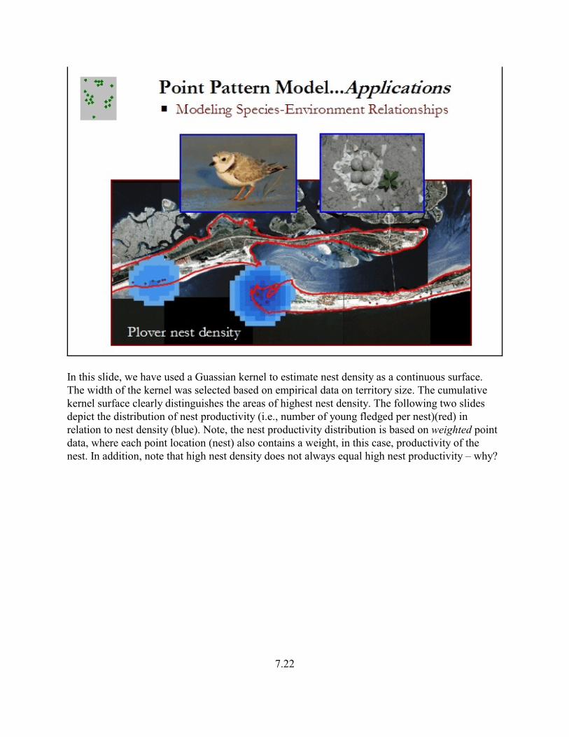
This slide shows the plover nest density kernel overlaid on the people on beech kernel and thereis some indication of an inverse relationship between nest density and people density (i.e., nestdensity increases where people density decreases). However, this relationship must be exploredstatistically before any inferences about the relationship can be made.

7.26

Lastly, we have used the point-based kernel approach to estimate the distribution of severalpoint-based environmental variables. Two others shown here are beach off-road vehicle (ORV)activity (where each ORV is recorded as a separate point location) and gull intensity (where eachrecorded gull is recorded as a separate point location). Gulls of several species are potentialpredators of plover chicks. Currently, we are using statistical procedures to examine therelationship between plover nest density and productivity and each of these and several otherenvironmental variables. The key point here is that point pattern analysis underpins most of ouranalysis into the plover-environment relationship.

7.27

2.6. Pros and Cons

Considering the information presented thus far, what are the strengths and limitations of the pointpattern model of landscape structure?

7.28

3. Patch Mosaic Model

3.1. Data Characteristics

The patch mosaic model represents data in which the system property of interest is represented asa mosaic of discrete patches that can be intuitively defined by the notion of "edge" (a patch is anarea with edges adjoining other patches). From an ecological perspective, patches representrelatively discrete areas of relatively homogeneous environmental conditions at a particular scale.The patch boundaries are distinguished by abrupt discontinuities (boundaries) in environmentalcharacter states from their surroundings of magnitudes that are relevant to the ecologicalphenomenon under. The patch mosaic model is the dominant model of landscape structure in usetoday. Familiar examples include:

• Map of land cover types• Map of ownership parcels

7.29

3.2. Data Structure

In the patch mosaic model, the data consists of polygons (vector) or grid cells (raster) classifiedinto discrete classes. There are many methods for deriving a categorical map of patches. Patchesmay be classified and delineated qualitatively through visual interpretation of the data (e.g.,delineating vegetation polygons through interpretation of aerial photographs), as is typically thecase with vector maps constructed from digitized lines. Alternatively, with raster grids,information at every location, typically obtained through remote sensing, may be used to classifycells into discrete classes and then to delineate patches by outlining them, and there are a varietyof methods for doing this.

7.30

3.3. Pattern Elements

In the patch mosaic model three major landscape elements are typically recognized: patches,corridors and matrix, and the extent and configuration of these elements defines the pattern ofthe landscape. The patch mosaic model is most powerful when meaningful patches can be clearlydefined and accurately mapped as discrete patches, and when the variation within a patch isdeemed relatively insignificant. The patch mosaic model assumes patches are homogeneouswithin (or treats them so) and categorically different from one another. For example, breedinghabitat for many pond-breeding amphibians can be clearly defined and delineated with relativelylittle uncertainty, and the variation in habitat quality within ponds is insignificant compared toamong-pond differences or pond-upland differences. Similarly, forested woodlots embeddedwithin a contrasting agricultural or urban landscape, fields in a forested landscape, stands ofdeciduous trees within a coniferous forest, and many other examples can be represented easilyand meaningfully in a categorical map. In general, whenever disturbances (natural oranthropogenic) either create discrete patches or leave behind discrete remnant patches, the patchmosaic model is likely to be useful.

7.31

(1) Patch

In the patch mosaic model, landscapes are composed of a mosaic of patches (Urban et al. 1987).Landscape ecologists have used a variety of terms to refer to the basic elements or units thatmake up a patch mosaic, including ecotope, biotope, landscape component, landscape element,landscape unit, landscape cell, geotope, facies, habitat, and site (Forman and Godron 1986). Anyof these terms, when defined, are satisfactory according to the preference of the investigator. Likethe landscape, patches comprising the landscape are not self-evident; patches must be definedrelative to the phenomenon under consideration. For example, from a timber managementperspective a patch may correspond to the forest stand. However, the stand may not function as apatch from a particular organism's perspective. From an ecological perspective, patches representrelatively discrete areas (spatial domain) or periods (temporal domain) of relatively homogeneousenvironmental conditions where the patch boundaries are distinguished by discontinuities inenvironmental character states from their surroundings of magnitudes that are perceived by orrelevant to the organism or ecological phenomenon under consideration (Wiens 1976). From astrictly organism-centered view, patches may be defined as environmental units between whichfitness prospects, or "quality", differ; although, in practice, patches may be more appropriatelydefined by nonrandom distribution of activity or resource utilization among environmental units,as recognized in the concept of "Grain Response".

7.32

Patches are dynamic and occur on a variety of spatial and temporal scales that, from an organism-centered perspective, vary as a function of each animal's perceptions (Wiens 1976 and 1989,Wiens and Milne 1989). A patch at any given scale has an internal structure that is a reflection ofpatchiness at finer scales, and the mosaic containing that patch has a structure that is determinedby patchiness at broader scales (Kotliar and Wiens 1990). Thus, regardless of the basis fordefining patches, a landscape does not contain a single patch mosaic, but contains a hierarchy ofpatch mosaics across a range of scales.

7.33

Patch boundaries are artificially imposed and are in fact meaningful only when referenced to aparticular scale (i.e., grain size and extent). For example, even a relatively discrete patchboundary between an aquatic surface (e.g., lake) and terrestrial surface becomes more and morelike a continuous gradient as one progresses to a finer and finer resolution. However, mostenvironmental dimensions possess one or more "domains of scale" (Wiens 1989) at which theindividual spatial or temporal patches can be treated as functionally homogeneous; atintermediate scales the environmental dimensions appear more as gradients of continuousvariation in character states. Thus, as one moves from a finer resolution to coarser resolution,patches may be distinct at some scales (i.e., domains of scale) but not at others.

7.34

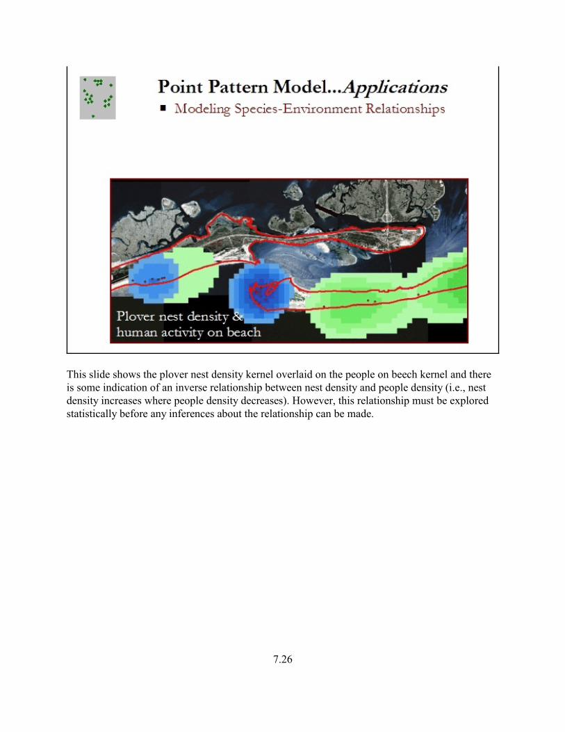
KEY POINT: It is not my intent to argue for a particular definition of patch. Rather, I wish topoint out the following: (1) that patch must be defined relative to the phenomenon underinvestigation or management; (2) that, regardless of the phenomenon under consideration (e.g.,a species, geomorphological disturbances, etc), patches are dynamic and occur at multiplescales; and (3) that patch boundaries are only meaningful when referenced to a particular scale.It is incumbent upon the investigator or manager to establish the basis for delineating amongpatches and at a scale appropriate to the phenomenon under consideration.

7.35

(2) Corridor

Corridors are linear landscape elements that can be defined on the basis of structure or function.Forman and Godron (1986) define corridors as “narrow strips of land which differ from thematrix on either side. Corridors may be isolated strips, but are usually attached to a patch ofsomewhat similar vegetation.” These authors focus on the structural aspects of the linearlandscape element and recognize three different types of structural corridors: (1) line corridors,in which the width of the corridor is too narrow to allow for interior environmental conditions todevelop; (2) strip corridors, in which the width of the corridor is wide enough to allow forinterior conditions to develop; and (3) stream corridors, which are a special category.Alternatively, these authors also classify corridors based on the agent of formation, including: (1)disturbance corridors, in which the corridor is established by a disturbance event, usuallyanthropogenic (e.g., roads, utility lines, fences); (2) remnant corridors, in which the corridor isthe result of disturbance around the corridor, leaving the corridor as an intact remnant of theformally widespread cover type; and (3) environmental corridors, in which the corridor is theresult of a strong linear environmental gradient, such as a riparian corridor created by the land-water interface along a stream.

7.36

As a consequence of their form and context, structural corridors may function as habitat,dispersal conduits, barriers, or as a source of abiotic and biotic effects on the surrounding matrix:

• Habitat Corridor.--Linear landscape element that provides for survivorship, natality, andmovement (i.e., habitat), and may provide either temporary or permanent habitat. Habitatcorridors passively increase landscape connectivity for the focal organism(s).

• Facilitated Movement Corridor.–Linear landscape element that provides for survivorship andmovement, but not necessarily natality, between other habitat patches. Facilitated movementcorridors actively increase landscape connectivity for the focal organism(s).

• Barrier or Filter Corridor.–Linear landscape element that prohibits (i.e., barrier) ordifferentially impedes (i.e., filter) the flow of energy, mineral nutrients, and/or species across(i.e., flows perpendicular to the length of the corridor). Barrier or filter corridors activelydecrease matrix connectivity for the focal process.

• Source of Abiotic and Biotic Effects on the Surrounding Matrix.–Linear landscape elementthat modifies the inputs of energy, mineral nutrients, and/or species to the surrounding matrixand thereby effects the functioning of the surrounding matrix.

7.37

Most of the past attention and debate has focused on facilitated movement corridors. It has beenargued that this corridor function can only be demonstrated when the immigration rate to thetarget patch is increased over what it would be if the linear element was not present (Rosenberget al. 1997). Unfortunately, as Rosenberg et al. point out, there have been few attempts toexperimentally demonstrate this. In addition, just because a corridor can be distinguished on thebasis of structure, it does not mean that it assumes any of the above functions. Moreover, thefunction of the corridor will vary among organisms due to the differences in how organismsperceive and scale the environment. More recently, the attention has shifted to the role ofcorridors as barriers or impediments to ecological flows.

KEY POINT: Corridors are distinguished from patches by their linear nature and can bedefined on the basis of either structure or function or both. If a corridor is specified, it isincumbent upon the investigator or manager to define the structure and implied function relativeto the phenomena (e.g., species) under consideration.

7.38

(3) Matrix

In the patch mosaic model, the matrix is the most extensive and most connected element, andtherefore plays the dominant role in the functioning of the landscape. For example, in a largecontiguous area of mature forest embedded with numerous small disturbance patches, the matureforest constitutes the matrix because it is greatest in extent, is mostly connected, and exerts adominant influence on the biota and ecological processes. In most landscapes the matrix isobvious to the investigator or manager. However, in some landscapes, or at a certain point intime, the matrix will not be obvious, and it may not be appropriate to consider any element as thematrix. The designation of a matrix is largely dependent upon the phenomenon underconsideration. For example, in the study of geomorphological processes, the geological substratemay serve to define the matrix and patches; whereas, in the study of vertebrate populations,vegetation structure may serve to define the matrix and patches. In addition, what constitutes thematrix is dependent on the scale of investigation or management. For example, at a particularscale, mature forest may be the matrix with disturbance patches embedded within; whereas, at acoarser scale, agricultural land may be the matrix with mature forest patches embedded within.

KEY POINT: A matrix element is not inherent to the landscape. It is incumbent upon theinvestigator or manager to determine whether a matrix element exists and should be designatedgiven the scale and phenomenon under consideration.

7.39

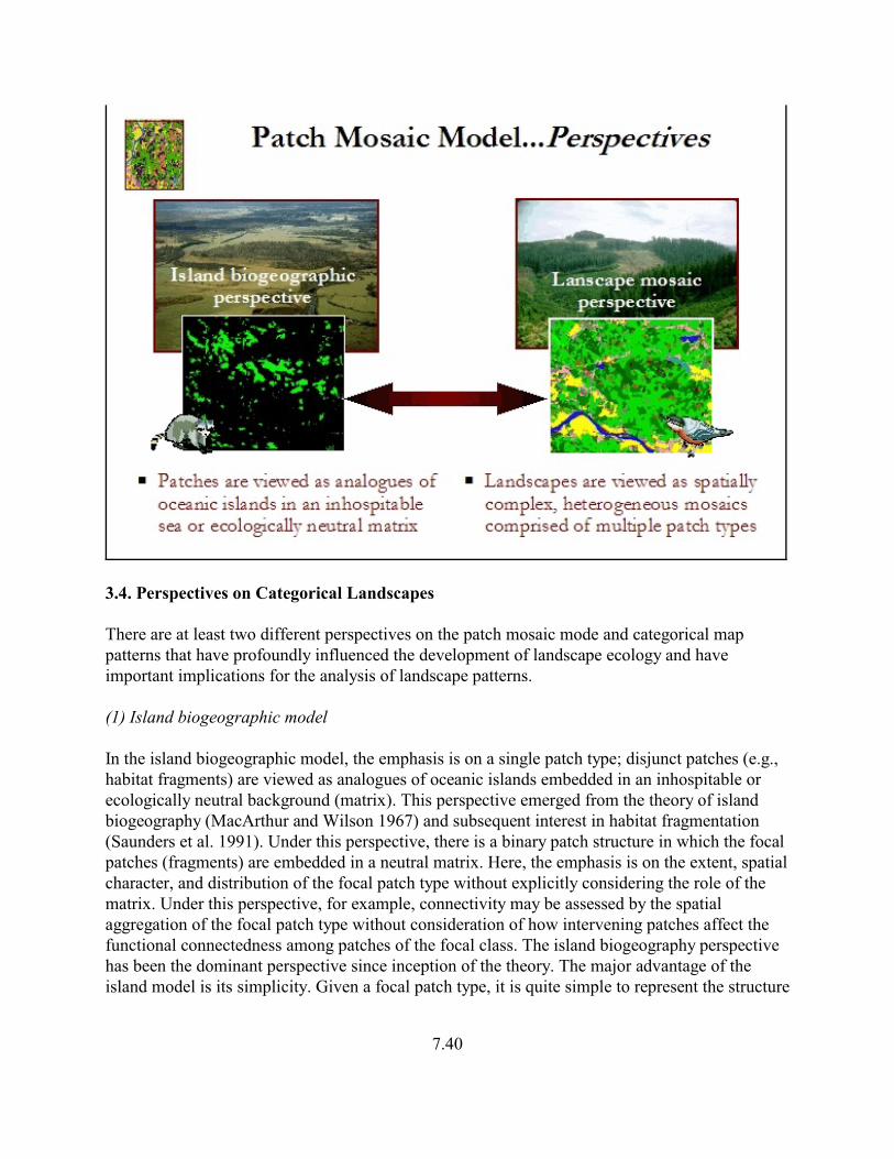
3.4. Perspectives on Categorical Landscapes

There are at least two different perspectives on the patch mosaic mode and categorical mappatterns that have profoundly influenced the development of landscape ecology and haveimportant implications for the analysis of landscape patterns.

(1) Island biogeographic model

In the island biogeographic model, the emphasis is on a single patch type; disjunct patches (e.g.,habitat fragments) are viewed as analogues of oceanic islands embedded in an inhospitable orecologically neutral background (matrix). This perspective emerged from the theory of islandbiogeography (MacArthur and Wilson 1967) and subsequent interest in habitat fragmentation(Saunders et al. 1991). Under this perspective, there is a binary patch structure in which the focalpatches (fragments) are embedded in a neutral matrix. Here, the emphasis is on the extent, spatialcharacter, and distribution of the focal patch type without explicitly considering the role of thematrix. Under this perspective, for example, connectivity may be assessed by the spatialaggregation of the focal patch type without consideration of how intervening patches affect thefunctional connectedness among patches of the focal class. The island biogeography perspectivehas been the dominant perspective since inception of the theory. The major advantage of theisland model is its simplicity. Given a focal patch type, it is quite simple to represent the structure

7.40

of the landscape in terms of focal patches contrasted sharply against a uniform matrix, and it isrelatively simple to devise metrics that quantify this structure. Moreover, by considering thematrix as ecologically neutral, it invites ecologists to focus on those patch attributes, such as sizeand isolation, that have the strongest effect on species persistence at the patch level. The majordisadvantage of the strict island model is that it assumes a uniform and neutral matrix, which inmost real-world cases is a drastic over-simplification of how organisms interact with landscapepatterns.

(2) Landscape mosaic model

In the landscape mosaic model, landscapes are viewed as spatially complex, heterogeneousassemblages of patch types, which can not be simply categorized into discrete elements such aspatches, matrix, and corridors (With 2000). Rather, the landscape is viewed from the perspectiveof the organism or process of interest. Patches are bounded by patches of other patch types thatmay be more or less similar to the focal patch type, as opposed to highly contrasting and oftenhostile habitats, as in the case of the island model. Connectivity, for example, may be assessed bythe extent to which movement is facilitated or impeded through different patch types across thelandscape. The landscape mosaic perspective derives from landscape ecology (Forman 1995) andhas only recently emerged as a viable alternative to the island biogeographic model. The majoradvantage of the landscape mosaic model is its more realistic representation of how organismsperceive and interact with landscape patterns. Few organisms, for example, exhibit a binary (allor none) response to habitats (patch types), but rather use habitats proportionate to the fitnessthey confer to the organism. Moreover, movement among suitable habitat patches usually is afunction of the character of the intervening habitats. The major disadvantage of the landscapemosaic model is that it requires detailed understanding of how organisms interact with landscapepattern, and this has delayed the development of additional quantitative methods that adopt thisperspective.

7.41

3.5. Pattern Metrics

Regardless of data format (raster or vector) and method of classifying and delineating patches,the goal of categorical map pattern analysis with such data is to characterize the composition andspatial configuration of the patch mosaic, and a plethora of metrics has been developed for thispurpose. We will explore these pattern metrics in detail in a subsequent lecture (and lab), so fornow, suffice it to say that there are many different metrics available for quantifying thecomposition and configuration of the patch mosaic. It is worth noting that in contrast to theemphasis on identifying the scale of pattern with point data and continuous data, so-calledscaling techniques for categorical map data are less commonly employed in landscape ecology.This may seem somewhat surprising given the predominant use of categorical data in landscapeecological investigations – after all, the predominant patch mosaic model of landscape structureis based on a categorical data format. However, there has been a plethora of landscape metricsdeveloped for quantifying various aspects of categorical map patterns and these have largelytaken the place of the more conventional scaling techniques. In addition, in applicationsinvolving categorical map patterns, the relevant scale of the mosaic is often defined a prioribased on the phenomenon under consideration. In such cases, it is usually assumed that it wouldbe meaningless to determine the so-called characteristic scale of the mosaic after its construction.

7.42

3.6. Applications

(1) Landscape ecological assessment

Landscape ecological assessment based on the patch mosaic model of landscape structure isincreasingly common. Given the inherent complexity of ecological systems and the dauntingchallenges confronting managers seeking to sustain ecosystems in the face of increasing humanpressures, it is not too surprising that managers are increasingly seeking effective ecologicalindicators. Landscape metrics that quantify the composition and configuration of the patchmosaic are increasingly being used as course-scale ecological indicators of change. In theexample shown here, several different pattern metrics were evaluated for their sensitivity to landuse change between 1974 and 1999 at Fort Benning, Georgia. In the realm of wetland ecologicalassessment there has been a similar explosion in the use of landscape pattern metrics to evaluatethe condition of wetlands as part of a regional wetlands monitoring and assessment program.While the current methods almost exclusively adopt pattern metrics based on the patch mosaicmodel of landscape structure, it is important to note that this is only by convention and thatmetrics derived from other conceptual models of landscape structure apply equally well.

7.43

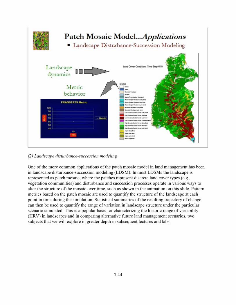
(2) Landscape disturbance-succession modeling

One of the more common applications of the patch mosaic model in land management has beenin landscape disturbance-succession modeling (LDSM). In most LDSMs the landscape isrepresented as patch mosaic, where the patches represent discrete land cover types (e.g.,vegetation communities) and disturbance and succession processes operate in various ways toalter the structure of the mosaic over time, such as shown in the animation on this slide. Patternmetrics based on the patch mosaic are used to quantify the structure of the landscape at eachpoint in time during the simulation. Statistical summaries of the resulting trajectory of changecan then be used to quantify the range of variation in landscape structure under the particularscenario simulated. This is a popular basis for characterizing the historic range of variability(HRV) in landscapes and in comparing alternative future land management scenarios, twosubjects that we will explore in greater depth in subsequent lectures and labs.

7.44

(3) Modeling species-environment relationships

Perhaps the most common application of pattern analysis based on the patch mosaic model is inmodeling species-environment relationships, and there are myriad examples of such applications.An increasingly common example involves quantifying the landscape structure around samplelocations for the purpose of building statistical models to explain and/or predict the distribution,abundance or performance of a species. In the example shown here, we adopted the patch mosaicmodel to map the distribution of several major cover types deemed potentially relevant to avariety of moth species in the pine barrens of southeastern Massachusetts. Conventionallandscape pattern analysis involves quantifying the structure of the entire landscape mosaic andreturning a single computed value for each metric.

7.45

However, in this study we were more interested in quantifying the local neighborhood structurearound each point location (represented as a cell in the raster grid). To do this, we passed amoving window of specified shape and size across the landscape one cell at time. Within eachwindow, we compute the desired landscape metric and returned the value to the focal (center)cell. By doing this for every cell in the input landscape, the result was a new grid depicting acontinuous surface representing the local landscape structure as measured by the particularmetric.

As shown in the next two slides, we repeated this process for several different landscape metricsat several different scales (i.e., window sizes). These local landscape structure surfacesrepresented independent variables in a logistic regression, where the dependent variable waspresence/absence of a particular moth species. Using statistical procedures, we identified thecombination of metrics and scales that best predicted each species presence/absence. Byoverlaying the predicted distribution of each species, we were able to identify areas of high mothrichness, which might serve to inform conservation decisions regarding where to focus landconservation efforts.

7.46

7.47

3.7. Pros and Cons

Considering the information presented thus far, what are the strengths and limitations of thepatch mosaic model of landscape structure?

7.48

4. Landscape Gradient Model

4.1. Data Characteristics

An alternative approach to the conventional patch mosaic model involves representingheterogeneity continuously – as a gradient. In this model, heterogeneity does not exist in discretepatches, but rather exists as a continuously varying property of the local environment andlandscape. Here, the data can be conceptualized as representing a three-dimensional surface,where the measured value at each geographic location is represented by the height of the surface.For example, instead of representing habitat as discrete patches, it is represented as a suitabilityor capability index, where the value at each location represents the quality of habitat and can takeon continuous values. In practice, habitat suitability or capability is often classified intocategories representing, say, high-, moderate-, and low-quality habitat, but this is more oftendone for convenience to facilitate further analysis with conventional categorical-basedprocedures or to simplify the presentation of results. Other familiar examples of inherentlycontinuous gradients include:

• Map of elevation• Map of burn severity• Map of leaf area index

7.49

4.2. Data Structure

Continuous surface pattern data typically are represented using a raster data structure, whereineach cell (or pixel) takes on a continuous value. Alternatively, it may be convenient in someapplications to represent continuous surface data using a vector data structure, wherein thesurface is represented as a series of contours (lines) as in the familiar topographic map.

7.50

4.3. Pattern Elements

Interestingly, there are no pattern elements in the landscape gradient model, making it the mostparsimonious of the landscape structure models.

7.51

4.4. Pattern Metrics

A wide variety of methods have been developed for quantifying the intensity and scale of patternin regionalized quantitative variables. Recall that a “regionalized” variable is one that takes onvalues based on its spatial location and that the analysis of the spatial dependencies (orautocorrelation – the ability to predict values of a variable from known values at other locations,as described by a ‘structure function’) in the measured characteristic is the purview ofgeostatistics. Recall that a variety of techniques exist for measuring the intensity and scale of thisspatial autocorrelation, and while the location of the data points (or quadrats) is known and ofinterest, it is the values of the measurement taken at each point that are of primary concern.

(1) Autocorrelation Structure Functions

The most basic and common measures of pattern in regionalized quantitative variables (i.e.,landscape gradients) are based on autocorrelation structure functions, including for exampleMoran’s I autocorrelation coefficient and semivariance, which we described previously as scalingtechniques for continuous gradient data. Both measures are typically used to describe themagnitude of autocorrelation as a function of distance between locations, as expressed by thecorrelogram and variogram (or semi-variogram), respectively, and illustrated here for a gradientin the topographic moisture index along a transect at the Coweeta Experiment Station.

7.52

(2) Other Structure Functions

There are many other methods for analyzing the intensity and scale of pattern with continuousdata, especially when the data is collected along continuous transects or two-dimensionalsurfaces, which we described previously as scaling techniques for continuous gradient data. Likethe autocorrelation structure functions, these techniques are typically used to quantify spatialdependencies in a quantitative variable in relation to scale (distance). Recall that no onetechnique has been found to be superior for all applications.

7.53

(3) Surface metrology metrics

The autocorrelation and other related structure functions described above can provide usefulindices to quantitatively compare the intensity and extent of autocorrelation in quantitativevariables among landscapes. However, while they can provide information on the distance atwhich the measured variable becomes statistically independent, and reveal the scales of repeatedpatterns in the variable, if they exist, they do little to describe other interesting aspects of thesurface. For example, the degree of relief, density of troughs or ridges, and steepness of slopesare not measured. Fortunately, a number of gradient-based metrics that summarize these andother interesting properties of continuous surfaces have been developed in the physical sciencesfor analyzing three-dimensional surface structures (Barbato et al. 1996, Sout et al. 1994,Villarrubia 1997). In the past ten years, researchers involved in microscopy and molecularphysics have made tremendous progress in this area, creating the field of surface metrology(Barbato et al. 1996).

7.54

In surface metrology, several families of surface pattern metrics have become widely utilized.One so-called family of metrics quantify intuitive measures of surface amplitude in terms of itsoverall roughness, skewness and kurtosis, and total and relative amplitude. Another familyrecords attributes of surfaces that combine amplitude and spatial characteristics such as thecurvature of local peaks. Together these metrics quantify important aspects of the texture andcomplexity of a surface. A third family measures certain spatial attributes of the surfaceassociated with the orientation of the dominant texture. A final family of metrics is based on thesurface bearing area ratio curve (or Abbott curve). The Abbott curve is computed by inversion ofthe cumulative height distribution histogram. The curve describes the distribution of mass in thesurface across the height profile. A number of indices have been developed from the proportionsof this cumulative height-volume curve which describe structural attributes of the surface.

Many of the patch-based metrics for analyzing categorical landscapes have analogs in surfacemetrology. For example, compositional metrics such as patch density, percent of landscape andlargest patch index are matched with peak density, surface volume, and maximum peak height.Configuration metrics such as edge density, nearest neighbor index and fractal dimension indexare matched with mean slope, mean nearest maximum index and surface fractal dimension. Manyof the surface metrology metrics, however, measure attributes that are conceptually quite foreignto conventional landscape pattern analysis. Landscape ecologists have not yet explored thebehavior and meaning of these new metrics; it remains for them to demonstrate the utility ofthese metrics, or develop new surface metrics better suited for landscape ecological questions.

7.55

McGarigal et al. (2009) examined landscapes in Turkey defined using both the landscapegradient and patch mosaic models according to a variety of landscape definition schemes andconducted multivariate statistical analyses to identify the universal, consistent and importantcomponents of surface patterns and their relationship to patch-based metrics. They observed fourrelatively distinct components of landscape structure based on empirical relationships among 17surface metrics across 18 landscape gradient models:

1. Surface roughness

The dominant structural component of the surfaces was actually a combination of two distinctsub-components: (1) the overall variability in surface height and (2) the local variability in slope.The first sub-component refers to the nonspatial (composition) aspect of the vertical heightprofile; that is, the overall variation in the height of the surface without reference to thehorizontal variability in the surface, and is represented by three surface amplitude metrics:average roughness (Sa), root mean square roughness (Sq), and ten-point height(S10z)(Appendix). These metrics are analogous to the patch type diversity measures (e.g.,Simpson's diversity index) in the patch mosaic paradigm, whereby greater variation in surfaceheight equates to greater landscape diversity. Importantly, while these metrics reflect overallvariability in surface height, they say nothing about the spatial heterogeneity in the surface.

7.56

The second sub-component refers to the spatial (configuration) aspect of surface roughness withrespect to local variability in height (or steepness of slope), and includes two surface metrics:surface area ratio (Sdr) and root mean square slope (Sdq)(Appendix). These metrics areanalogous to the edge density and contrast metrics (e.g., contrast-weighted edge density, totaledge contrast index) in the patch mosaic paradigm, whereby greater local slope variation equatesto greater density and contrast of edges. Interestingly, while these surface metrics reflectsomething akin to edge contrast, they do so without the need to supply edge contrast weightsbecause they are structural metrics. These two metrics appear to have the greatest overall analogyto the patch-based measures of spatial heterogeneity and overall patchiness. A fine-grained patchmosaic (as represented by any number of common patch metrics, such as mean patch size ordensity) is conceptually equivalent to a rough surface with high local variability.

On conceptual and theoretical grounds, these spatial and nonspatial aspects of surface roughnessare independent components of landscape structure; however, in the landscape gradients weexamined these two aspects were highly correlated empirically. This distinction betweenconceptually and/or theoretically related metrics and groupings based on their empirical behaviorhas also been demonstrated for patch metrics.

7.57

2. Shape of the surface height distribution

Another important nonspatial (composition) component of the surfaces we examined was theshape of the surface height distribution. This component was comprised of five metrics:skewness (Ssk), kurtosis (Sku), surface bearing index (Sbi), valley fluid retention index (Svi),and core fluid retention index (Sci). All of these metrics measure departure from a Gaussiandistribution of surface heights, but emphasize different aspects of departure from normality(Appendix). Ssk and Sku measure the familiar skewness and kurtosis of the surface heightdistribution, while the surface bearing metrics, Sbi, Sci and Svi, measure different aspects of thesurface height distribution in its cumulative form. This component was universally present acrosslandscape models, but the composition of metrics varied somewhat among models reflecting thecomplexities inherent in measuring non-parametric shape distributions. There were no strongpatch mosaic analogs to these surface metrics; however, departure from a Gaussian distributionof surface heights was weakly correlated with, and conceptually most closely related to,patch-based measures of landscape dominance (or its compliment, evenness) such as Simpson'sevenness index (SIEI) and largest patch index (LPI). Importantly, these five surface metricsmeasure the 'shape' of the surface height distribution and are not affected by the surfaceroughness (as defined above) per se.

7.58

3. Angular texture

A third prominent component of the surfaces we examined was the angular orientation(direction) of the surface texture and its magnitude. This component is inherently spatial, sincethe arrangement of surface peaks and valleys determines whether the surface has a particularorientation or not, and is represented by four spatial metrics: dominant texture direction (Std),texture direction index (Stdi), and two texture aspect ratios (Str20 and Str37). The computationalmethods behind these metrics are too complex to describe here (but see Appendix), but are basedon common geostatistical methods (Fourier spectral analysis and autocorrelation functions) thatdetermine the degree of anisotropy (orientation) in the surface. Not surprisingly given ourknowledge of the study landscape, we did not observe sample landscapes with a strong textureorientation. We did observe mild levels of texture orientation in some landscapes, but many werewithout apparent orientation. Importantly, the measurement of texture direction has no obviousanalog in the patch mosaic paradigm; indeed, we observed no pairwise correlation greater than±0.22 between any of these four surface metrics and any of the 28 patch metrics.

7.59

4. Radial texture

The fourth prominent component of the surfaces we examined was the radial texture of thesurface and its magnitude. Radial texture refers to repeated patterns of variation in surface heightradiating outward in concentric circles from any location. Like angular texture, this component isinherently spatial, since the arrangement of surface peaks and valleys determines whether thesurface has any radial texture or not, and is represent by three spatial metrics: dominant radialwavelength (Srw), radial wave index (Srwi), and fractal dimension (Sfd). Again, thecomputational methods behind these metrics are based on common geostatistical methods. Alimitation of these and other metrics based on Fourier spectral analysis and autocorrelationfunctions is that they are only sensitive to repeated, regular patterns. We observed that in theabsence of a prominent radial texture, the dominant radial wavelength (Srw) ends up being equalto the diameter of the sample landscape. As a result, in some of our landscape gradient modelswe observed too little variation in this metric and were forced to drop it from the final analyses.Despite these limitations, we observed sample landscapes with varying degrees of radial texturebased on the other two metrics. In contrast to angular texture, the measurement of radial texturehas at least one conceptual analog in the patch mosaic paradigm - mean and variability in nearestneighbor distance. On conceptual grounds, Srw should equate to mean nearest neighbor distance,and Srwi and Sfd should equate to the coefficient of variation in nearest neighbor distance.However, in our study the corresponding pairwise correlations did not exceed ±0.22, nor werethere any pairwise correlations greater than ±0.40 between either of these surface metrics and anyof the 28 patch metrics.

7.60

4.5. Applications

(1) Scaling gradient patterns

By far the most common application of surface pattern metrics in landscape ecology has been toidentify the characteristic scale or scales of the ecological phenomena or to elucidate the natureof the scaling relationship. One thing that is true of pattern, as we have already seen, is that itsexpression varies with scale. Thus, a careful evaluation of the relationship between scale andpattern is often considered an important first step in the characterization of pattern. In addition,we noted previously, quantifying the scaling relationship of the ecological phenomenon ofinterest can provide unique insights into potential pattern-process relationships. For example,multi-scaled patterns (i.e., those with two or more distinctive characteristic scales) revealedthrough scaling techniques can indicate the existence of multiple agents of pattern formationoperating at different scales. Conversely, scaling techniques can be used to assess a priorihypotheses concerning agents of pattern formation; e.g., is the expected scale or scales of patternexpressed in the data?

7.61

In the example shown here, semivariance was used to examine the scale of pattern in theabundance of coastal cutthroat trout in several Pacific Northwest streams. In this case, theregionalized quantitative variable of interest is fish abundance and the spatial lag is streamdistance; i.e., the distance between two points on the stream along the flow path. Thesemivariograms reveal different patterns of variation among streams. For example, the pattern ofvariation for Glenn Creek in the Coast Range shows a distinct sill with a range of approximately1100 m. In contrast, the pattern for Miller Creek in the Cascade Range reveals a nested patchypattern with a gradient; that is, a distinct scale of patchiness at roughly 300-400 m superimposedon a coarse-scale gradient of increasing dissimilarity in fish abundance with increasing streamdistance. These patterns may reveal something about the differences between these streamsystems in the underlying distribution of habitat (e.g., the distribution of channel unit types).

7.62

In the example shown here (from Meador et al. 2009), continuing with the example shown earlierin the point pattern analysis section, correlograms were used to discern the pattern of spatialautocorrelation in tree diameter (dbh) as a proxy fo establishment age in historical forest stands(pre-European land use) versus contemporary forest stands (post-European land use) inponderosa pine forests of northern Arizona. In all cases, there was strong autocorrelation outto15-30 m in the pre-1894 and contemporary stands, which the authors interpreted as evidence ofthe “clumpy-groupy” nature of tree establishment, whereby trees establish in small groups largelyin the openings between the patches of canopy.

7.63

They also estimated tree establishment age for all the historical trees and contemporary trees andfit a semivariogram to the data (as shown) and then used the process of krigging to create aninterpolated surface of tree establishment age. In the figure shown here, the colored areasrepresent contours of tree establishment age, with the immediate post-harvest 1909 residual treesshown as points (with the symbol sized proportionate to dbh). The pattern reveals that treeslargely established in cohorts up until the last regeneration event in 1953 and established first inthe openings in clumps/groups and then gradually established closer to the existing canopies andlastly underneath the existing canopy.

7.64

(2) Landscape disturbance-succession modeling

Another application of landscape gradient model in land management has been in landscapedisturbance-succession modeling (LDSM). As noted previously, most LDSMs adopt the patchmosaic model of landscape structure; however, some models utilize a gradient-based approach ora hybrid approach in which some aspects of the landscape are represented as a continuoussurface. For example, the LANDIS model represents vegetation as a continuous surface whereeach cell can take on continuous values for the abundance of each tree species and age cohort.Disturbance and succession processes operate in various ways to alter the distribution ofindividual species and age cohorts over time, essentially modifying the continuous surfacestructure in species abundance and age. Simple landscape composition metrics that quantify thetotal area occupied by each species and age class can then be computed for each timestep of themodel and summarized for the simulation as a whole. And while surface metrology metrics havenot yet been employed to describe the changing landscape structure in connection with thissimulation model, the potential exists to do so.

7.65

(3) Modeling pattern-process relationships

There are myriad possibilities for using the landscape gradient model to explore pattern-processrelationships, which we will illustrate here with a couple of examples.

In the first example, Moody et al. (2007) used the gradient model to examine the relationshipbetween burn severity and runoff after a large wildfire. Extreme floods often follow wildfire inmountainous watersheds. However, a quantitative relation between the runoff response and burnseverity at the watershed scale has not been established. Runoff response was measured as therunoff coefficient C, which is equal to the peak discharge per unit drainage area divided by theaverage maximum 30 min rainfall intensity during each rain storm. The magnitude of the burnseverity was expressed as the change in the normalized burn ratio, a continuous surface derived

ifrom LandsatTM imagery. A new burn severity variable, hydraulic functional connectivity Ç wasdeveloped and incorporates both the magnitude of the burn severity and the spatial sequence ofthe burn severity along hillslope flow paths. The runoff response and the burn severity weremeasured in seven subwatersheds in the upper part of Rendija Canyon burned by the 2000 CerroGrande Fire near Los Alamos, New Mexico, USA. The runoff coefficient was a linear function ofthe mean hydraulic functional connectivity of the subwatersheds. Moreover, the variability of themean hydraulic functional connectivity was related to the variability of the mean runoffcoefficient, and this relation provides physical insight into why the runoff response from thesame subwatershed can vary for different rainstorms with the same rainfall intensity.

7.66

In the second example, Cushman et al. (2006) used the gradient model to examine therelationship between gene flow and landscape structure in black bears in northern Idaho. Theytested several hypotheses about environmental factors affecting gene flow, including thehypothesis that observed gene flow was best explained by landscape resistance represented as acontinuous surface based on a factorial combination of elevation, slope, vegetative cover, androads. Here, landscape resistance derived from multiple environmental attributes was portrayedas a continuous surface using the landscape gradient model of landscape structure. As will beexplained in more detail in a subsequent lecture, they used statistical procedures to compare thegenetic distance among the individual bears sampled across the landscape to the ecologicaldistance among sample locations based on least cost distances derived from the resistantlandscape surface.

7.67

4.6. Pros and Cons

Considering the information presented thus far, what are the strengths and limitations of thelandscape gradient model of landscape structure?

7.68

5. Graph matrix model

5.1. Data Characteristics

An altogether different approach for representing landscape structure that in many ways adoptsaspects of all the preceding models is based on graph theory. In the graph-theoretic model, thedata consists of a collection of nodes (patches) and linkages (connections) represented as datamatrices. In this model, the landscape is simplified into a graph depicting the focal points orpatches as the nodes and the linkages between nodes as connections. In the example shown here,the grass openings, representing habitat patches, are the nodes and the shortest pathway betweenpatches are the links. Graph theory is widely used in computer science and engineering, andbecame popular in food-web theory and landscape ecology in the early 90's. In landscapeecology, graph theory has been described as a tool that bridges the gap between structuralmeasures and functional measures of a landscape, where it has been proven useful in examiningconnectivity and ecological flows.

7.69

5.2. Data Structure

The graph-matrix model is distinctive in representing the landscape structure as a set of datamatrices, wherein the spatial heterogeneity is summarized in two non-spatial data matrices:

1. Node data matrix – contains the x,y coordinates of the nodes and may also contain additionalinformation about the nodes such as the size and/or quality of the patch.

2. Link data matrix – square matrix containing information pertaining to the links betweenevery pair of nodes. There are at least three different sorts of edge matrices possible:a. Distance matrix – containing ecological distances between every pair of nodes, based on

simple Euclidean distance or functional distance, for example using least cost pathsderived from resistance surfaces. In addition, distances can be from nearest patch edge topatch edge or from patch centroid to patch centroid.

b. Flux/Dispersal probability matrix – containing rates of ecological flow (e.g., dispersal)between every pair of nodes, derived from the distance matrix by applying some functionto the distance, from some attribute of the nodes (e.g., patch size, population size), orfrom empirical data collected in the field.

c. Adjacency matrix – binary indicator matrix containing 0's for disconnected links and 1'sfor connected links. The adjacency matrix could be created from either of above matricesusing a threshold distance to define connectivity.

7.70

5.3. Pattern Elements

Graph matrices contain two basic elements: nodes and links.

1. Nodes – nodes (also referred to as vertices) can represent any point or patch features of thelandscape relevant to the phenomenon under consideration. It is important to recognize that in thegraph nodes are depicted as points, but in reality they may represent patches of widely varyingsizes. In most cases, the patch centroid is used to represent the patch location in the graph.

2. Links – links (also referred to as edges in the graph theoretic framework) represent theconnections between nodes. Again, it is important to recognize that in the graph links aredepicted as straight lines between nodes, but in reality they may represent nonlinear pathwaysbetween nodes or flux rates between nodes that don’t have an explicit spatial representation.Moreover, the links can have directionality; that is, the distance or flux rate between two nodesmay not be the same in both directions. For example, if flux rate is influenced by gravitationalfields, then the “distance” between node A downslope and node B upslope may dependdramatically on whether the link as from A to B or the reverse.

7.71

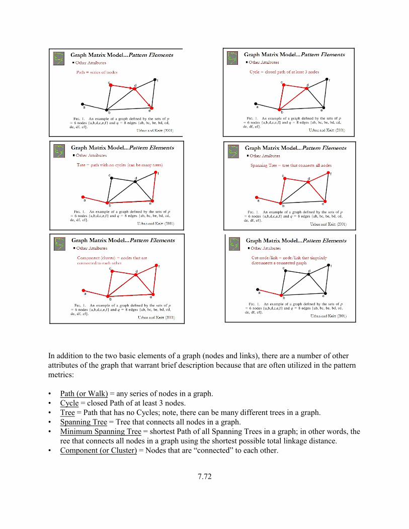
In addition to the two basic elements of a graph (nodes and links), there are a number of otherattributes of the graph that warrant brief description because that are often utilized in the patternmetrics:

• Path (or Walk) = any series of nodes in a graph.• Cycle = closed Path of at least 3 nodes.• Tree = Path that has no Cycles; note, there can be many different trees in a graph.• Spanning Tree = Tree that connects all nodes in a graph.• Minimum Spanning Tree = shortest Path of all Spanning Trees in a graph; in other words, the

ree that connects all nodes in a graph using the shortest possible total linkage distance.• Component (or Cluster) = Nodes that are “connected” to each other.

7.72

• Cut-node/Cut-link = a Node/Link that singularly disconnects a connected graph.

5.4. Pattern Metrics

Not surprisingly, there are many ways to measure the differences between graphs. Here, wereview some of the more common ones:

• Number = number of components (disjunct clusters) in a graph.• Order = number of nodes in the largest component.• Diameter = diameter of the largest component, where diameter is defined as the “distance”

between the two nodes furthest apart and the path taken is always the shortest (also called theMaximum Eccentricity).

• Expected cluster size = area-weighted mean component (cluster) size, where the componentsize is defined as the total area contained in the corresponding nodes.

• Correlation length = area-weighted mean component (cluster) radius of gyration, where theradius of gyration is defined as the mean distance between each point or cell in a cluster andthe centroid of the cluster. Note, this measure is conceptually very similar to expected clustersize, but uses the average distance traversed within a cluster as opposed to the absolute areaof the cluster. Thus, the unit of measurement is a distance instead of an area.

7.73

• Connected graph = logical or binary indicator of whether all nodes are connected to all othernodes or not.

• Node-connectivity = number of nodes that need to be removed to disconnect a connectedgraph.

• Edge-connectivity = number of links that need to be removed to disconnect a connectedgraph.

7.74

It is important to remember that graph links can be defined on the basis of any measure ofecological distance, univariate or multivariate, and it is this feature that provides great flexibilityto the graph matrix model.

7.75

5.5. Applications

(1) Examining connectivity thresholds

The vast majority of applications have involved examining connectivity thresholds using amixture of both theoretical and empirical approaches. Let’s begin with a brief theoreticalexample fro Urban and Keitt (2001). One way to explore connectivity thresholds is tosequentially remove links by progressively decreasing the threshold distance for determiningwhether nodes are connected or not – the so called “edge thinning” approach. In the hypotheticalexample shown here, the graph is nearly connected at a threshold of 1500 m – there are but twocomponents (clusters). As the threshold distance is progressively decreased, the graph isincreasingly fragmented into a larger number of smaller components.

7.76

The structural changes in the graph occurring during this edge thinning experiment are shownhere. Specifically, the figure shown here depicts the changes in the number of components(number), number of nodes in the largest remaining component (order), and diameter of thelargest remaining component (diameter). As edges are progressively loss, moving from the rightto the left on the graph, at first there is no change in the metrics. This is because the edge-connectivity of the graph is greater than one, which means that each node is connected bymultiple links to other nodes so that the loss of any one link does not effect the overallconnectivity of the graph. However, at some point the diameter of the largest component goes upbefore eventually going down, which seems counter-intuitive at first. This happens because thedirect paths between nodes are lost at first- then stepping stones are lost. Thus, the cluster orderremains the same (i.e., no nodes are lost), but the shortest pathway between the two furthest apartnodes (diameter) increases. As links continue to be lost, at some point there is a rather abruptchange in all of the metrics. This threshold-like behavior reflects sudden and dramatic changes inthe connectivity of the graph as the connected graph begins to get fragmented into many smallercomponents. Ecologically, the implications are obvious – there may be critical ecologicaldistances (e.g., dispersal distances) that once crossed dramatically reduce connectivity of thelandscape.

7.77

An alternative way to explore connectivity thresholds is to sequentially remove nodes – the socalled “node thinning” approach. In the hypothetical example shown here, nodes wereprogressively removed using three different approaches: (1) randomly, (2) the smallest nodes (interms of area), and (3) the end-node with the smallest area. The right-hand figure shows therelationship between the number of nodes removed under the three removal methods and thegraph diameter. There were a couple of important findings from this study. First, the exact shapeof the resulting curves was landscape dependent, preventing generally applicable conclusions.Second, in this particular landscape, end-node removal showed an advantage over the otherremoval methods and exhibited threshold behavior, suggesting that node position in thelandscape can be important and that connectivity may change abruptly with the loss of criticalnodes.

7.78

Now let’s consider an empirical example. In the example shown here, the graph matrix modelwas used to examine connectivity thresholds in winter habitat of woodland Caribou in Manitoba,Canada (O’Brien et al. 2006). Caribou, a threatened species in Canada, require lichen-rich,mature conifer habitat, especially in winter. Past forestry practices have favored white-tailed deerand moose over caribou, though caribou can adapt to some habitat fragmentation as long asenough connected habitat is provided.

7.79

In this study, the graph matrix model was used to depict the distribution of high-quality winterhabitat patches and the potential linkages between those patches using data from 20 radio-collared animals. More specifically, nodes were defined as high-quality (lichen-rich jack pine andsparsely treed rock) winter habitat patches >5 ha. It is worth noting that this approach essentiallytreats all other land cover as non-habitat that is only traversed to get between habitat patches.This may or may not be a reasonable assumption. Links were defined as the least-cost pathwaysbetween habitat patches, where cost was based on a resource selection function derived usinglogistic regression.

7.80

The figure shown here depicts the relationship between expected cluster size (defined earlier),interpreted as a measure of overall landscape connectivity, and the cost distance based on leastcost pathways. Several things are evident in this figure. First, habitat patches connect graduallyover small scales, with large increases in ECS occurring at cost distances of 800, 1600 and 2250.These correspond to Euclidean distances of approximately 650 m, 1250 m, and 1750 m,respectively. These thresholds represent scales where the graph includes sub-clusters connectedby only a few links into one much larger cluster. Second, at a cost distance of roughly 2500 m(approximately 2000 m Euclidean distance), the graph is completely connected (i.e., all habitatpatches are connected into a single large cluster). Third, the curve for the late winter habitat useis greater than the curve for all winter and very close to the curve for the maximum cluster size,indicating that late winter animals utilize the largest available habitat clusters.

7.81

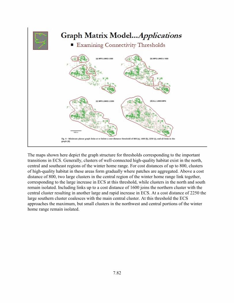
The maps shown here depict the graph structure for thresholds corresponding to the importanttransitions in ECS. Generally, clusters of well-connected high-quality habitat exist in the north,central and southeast regions of the winter home range. For cost distances of up to 800, clustersof high-quality habitat in these areas form gradually where patches are aggregated. Above a costdistance of 800, two large clusters in the central region of the winter home range link together,corresponding to the large increase in ECS at this threshold, while clusters in the north and southremain isolated. Including links up to a cost distance of 1600 joins the northern cluster with thecentral cluster resulting in another large and rapid increase in ECS. At a cost distance of 2250 thelarge southern cluster coalesces with the main central cluster. At this threshold the ECSapproaches the maximum, but small clusters in the northwest and central portions of the winterhome range remain isolated.

7.82

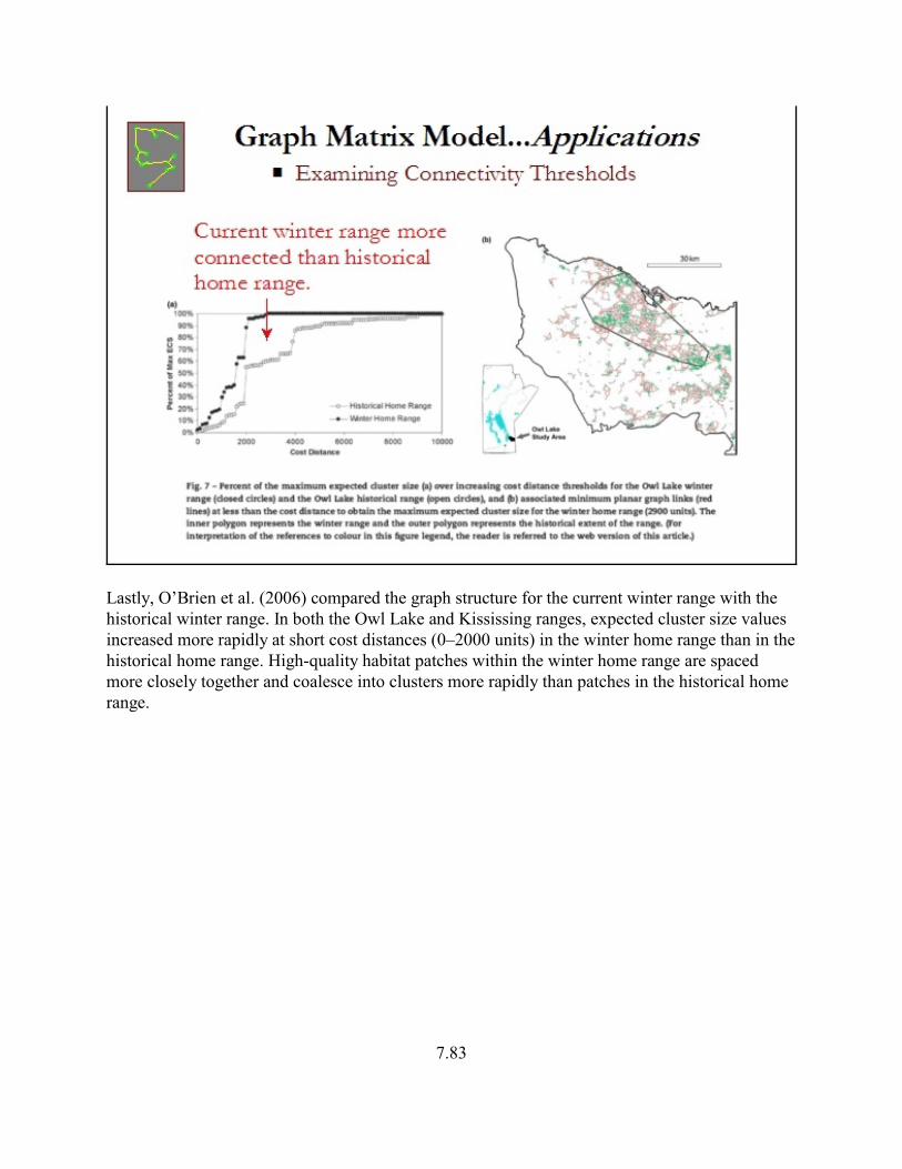
Lastly, O’Brien et al. (2006) compared the graph structure for the current winter range with thehistorical winter range. In both the Owl Lake and Kississing ranges, expected cluster size valuesincreased more rapidly at short cost distances (0–2000 units) in the winter home range than in thehistorical home range. High-quality habitat patches within the winter home range are spacedmore closely together and coalesce into clusters more rapidly than patches in the historical homerange.

7.83

(2) Identifying critical linkages

A closely related application of graph theory involves not only examining connectivity thresholdsbut identifying the critical linkages and/or nodes associated with threshold changes inconnectivity. In the classic study by Keitt et al. (1997), the authors used the graph matrix modelto represent habitat patches of the Mexican spotted owl in Colorado, Utah, Arizona and NewMexico. The links were simply Euclidean distances between patches.

7.84

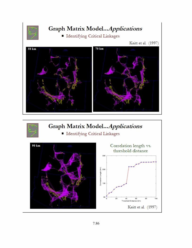
In the following series of figures, habitat patches are depicted in yellow and the links are inpurple. In the first figure, all links < 10 km are highlighted. The graph is highly disconnected.The second figure depicts all links <30 km. The graph is more connected, but still largelycomprised of several separate clusters. The next three figures depict the graph structure forthreshold distances of 50, 70 and 90 km. By definition, the correlation length of the graph(defined above) increases monotonically with increasing threshold distance. However, the graphshows a distinct threshold in the vicinity of 40 km, where correlation length almost doubles asthe threshold distance increases slightly. Interestingly, 40 km corresponds roughly to thedispersal distance of juvenile spotted owls.

7.85

7.86

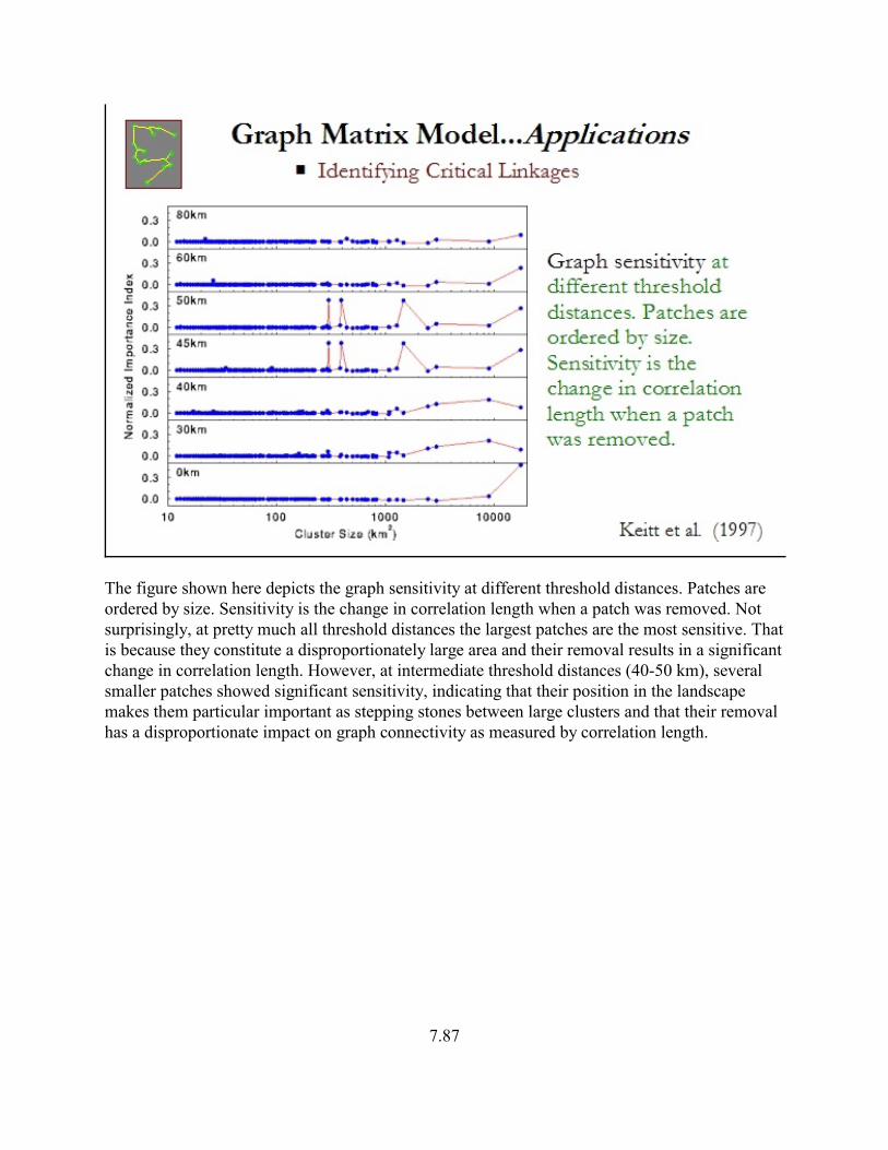
The figure shown here depicts the graph sensitivity at different threshold distances. Patches areordered by size. Sensitivity is the change in correlation length when a patch was removed. Notsurprisingly, at pretty much all threshold distances the largest patches are the most sensitive. Thatis because they constitute a disproportionately large area and their removal results in a significantchange in correlation length. However, at intermediate threshold distances (40-50 km), severalsmaller patches showed significant sensitivity, indicating that their position in the landscapemakes them particular important as stepping stones between large clusters and that their removalhas a disproportionate impact on graph connectivity as measured by correlation length.

7.87

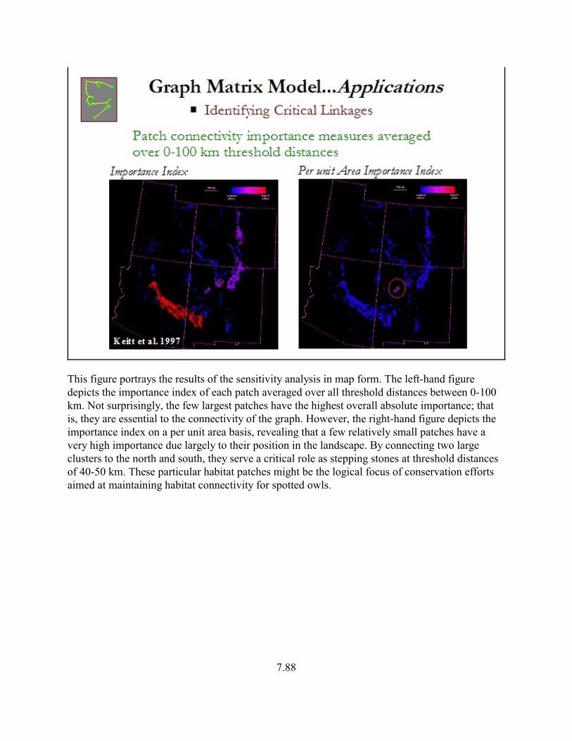
This figure portrays the results of the sensitivity analysis in map form. The left-hand figuredepicts the importance index of each patch averaged over all threshold distances between 0-100km. Not surprisingly, the few largest patches have the highest overall absolute importance; thatis, they are essential to the connectivity of the graph. However, the right-hand figure depicts theimportance index on a per unit area basis, revealing that a few relatively small patches have avery high importance due largely to their position in the landscape. By connecting two largeclusters to the north and south, they serve a critical role as stepping stones at threshold distancesof 40-50 km. These particular habitat patches might be the logical focus of conservation effortsaimed at maintaining habitat connectivity for spotted owls.

7.88

5.6. Pros and Cons

Considering the information presented thus far, what are the strengths and limitations of thegraph matrix model of landscape structure?

7.89