How much is enough? Requisite modelling for socio-technical problems
Modelling the socio-economic impact of implementing innovative infrastructure and rolling stock concepts on railway
Trans-European Corridors
Claudio Lombardi
Thesis to obtain the Master of Science Degree in
Civil Engineering
Supervisor: Professor Paulo Manuel da Fonseca Teixeira
Examination Committee
Chairperson: Professor João Torres de Quinhones Levy
Supervisor: Professor Paulo Manuel da Fonseca Teixeira
Members of the Committee: Professor Maria do Rosário Maurício Ribeiro Macário
September 2016

i
AKNOWLEDGMENTS
This thesis marks the end of my Master studies, started in Milan in October 2013. Some months after, I took the
decision to come to Lisbon, where this thesis was written.
This work was performed in the framework of the Capacity4rail EU research project. I had the privilege to be involved
in this project thanks to my supervisor from Instituto Superior Técnico, professor Paulo Teixeira. I really thank him for
this opportunity and for his constant help in finding and exploiting my margins of improvement.
I am also indebted to Frederico Francisco, PhD, from Instituto Superior Técnico research team in charge for
Capacity4rail. Without his permanent availability and his solid awareness, this work would not have been possible.
I also thank my Italian supervisor from Politecnico di Milano, professor Roberto Maja. Despite the distance, he always
followed my progress in the work, giving valid advice.
There are also many other people in the backstage that deserve to be thanked.
First of all my parents: I want to thank you for the chances you allowed me to take in life, supporting me with your
money and words. You also felt personally my stress during my academic path and the writing of this thesis.
Renan, thank you too. Living side by side with me, you felt, more than anyone else, my stress and you were always
there to encourage me. I am thankful to you for this.
Jessica, you also deserve to be thanked at the beginning of this work. You were the first person to receive any news
about its progess, usually while eating a fat Portuguese cake at Técnico Cafeteria and you were also there to
encourage me and stimulating to work on it.
Thank you Angelica, you were also constantly updated about my progress via super-long voice messages and you
encouraged me with other super-long voice messages.
I also want to thank the people that spent these last months with me and demonstrated care in trying to know how
the work was going and gave some encouragement to me: my dear friends Laura and Cristina, my cousins Mattia, Alba
and Sara, my friends Carmela, Solène, Mariangela, Pilar, Giorgia, Dario and Xavi and everyone else.
Thank you all for your support.
ii
ABSTRACT AND KEYWORDS
Transport constitutes a key sector of European economy as well as a major contributor to economy itself.
European Union set challenging goals in its transport policy, collecting them in its White Papers on transport.
These objectives, especially congestion and Green-House Gases emissions reductions cannot be achieved without the
solution of the main European railways current challenges: scarcity of capacity, lack of reliability and low travel
competitiveness.
Manifold are the projects currently under development regarding railways world in response to these challenges,
including the development of TEN-T projects.
Many research projects are also supported by European funds. Among them there is Capacity4Rail.
Due to their global character, these projects need the building of new tools to allow the assessment of the profitability
of the investments, which constitutes a major concern of EC policy, especially in a period of global crisis as the one we
are living.
The main aim of this work is indeed to cooperate with the Instituto Superior Técnico researchers’ team in establishing
a methodology to assess the socio-economic impact of innovations developed within the framework of the European
Project Capacity4rail.
After a revision of the current practices on railway infrastructure project appraisal, the methodology elaborated in
partnership with IST research team in charge for C4R is presented, highlighting what differentiates it from a common
Cost-Benefits Analysis, in particular the solution to the scarcity and uncertainty of input data and the evaluation of
capacity occupation and extreme events consequences in terms of delays.
An example of application of the elaborated methodology to the Swedish part of the TEN-T Scandinavian-
Mediterranean corridor is then presented.
Eventually, inputs on further requirements and improvability of the approach developed are provided, in particular
the extension of the approach to bigger sections of corridors is also considered, with regards to the necessary
modifications.
Keywords: White papers, European Transport Policy, TEN-T, Capacity4Rail, Cost-Benefit Analysis, Capacity Occupation,
Delays, Scan-Med corridor
iii
RESUMO E PALAVRAS-CHAVES
Os transportes constituem um sector-chave da economia europeia, bem como um dos principais contribuintes para a
própria economia.
A União Europeia estabeleceu metas desafiadoras na sua política de transportes, recolhendo-as nos Livros Brancos
sobre os transportes.
Estes objectivos, em particular o congestionamento e as reduções das emissões de gases com efeito de estufa, não
podem ser alcançados sem a solução dos principais desafios atuais das ferrovias europeias: escassez de capacidade,
falta de fiabilidade e baixa competitividade do tempo de viagem.
Vários são os projetos atualmente em desenvolvimento sobre ferrovias em resposta a estes desafios, incluindo o
desenvolvimento dos projectos RTE-T.
Muitos projetos de investigação também são apoiados por fundos da União Europeia. O Capacity4Rails está entre
eles.
Devido ao seu carácter global, estes projectos precisam da construção de novas ferramentas para permitir a avaliação
da rentabilidade dos investimentos, o que constitui uma das principais preocupações da política da Comissão
Europeia, especialmente num período de crise mundial como o que estamos a viver.
O principal objectivo desta dissertação é, de facto, a cooperação com a equipa de pesquisadores do Instituto Superior
Técnico no estabelecimento de uma metodologia para avaliar o impacto sócio-económico das inovações
desenvolvidas no âmbito do Projecto Europeu Capacity4rail.
Depois de uma revisão do estado da arte sobre a avaliação dos projetos de infra-estruturas ferroviárias, a
metodologia, elaborada em parceria com a equipa de investigação do IST encarregada de C4R, é apresentada,
destacando o que a diferencia de uma Análise Custos-Benefícios comum, em particular, a solução para a escassez e
incerteza dos dados de entrada e a avaliação das consequências da ocupação da capacidade e dos eventos extremos
em termos de atrasos.
Um exemplo de aplicação da metodologia elaborada à parte sueca do corredor RTE-T Escandinavo-Mediterrânico é
então apresentado.
Finalmente, pistas sobre outros requisitos e melhoramentos da abordagem desenvolvida são fornecidas, em particular
a extensão da abordagem a secções maiores de corredores também é considerada, no que diz respeito às
modificações necessárias.
Palavras-chave: White papers, Política europeia de transportes, RTE-T, Capacity4Rail, Análise Custo-Benefício,
Ocupação da Capacidade, Atrasos, Corredor Scan-Med
iv
INDEX
AKNOWLEDGMENTS ............................................................................................................................................................ i
ABSTRACT AND KEYWORDS ................................................................................................................................................ ii
RESUMO E PALAVRAS-CHAVES .......................................................................................................................................... iii
INDEX ................................................................................................................................................................................. iv
LIST OF TABLES ..................................................................................................................................................................viii
LIST OF GRAPHS ................................................................................................................................................................. ix
LIST OF FIGURES ................................................................................................................................................................. ix
LIST OF ABBREVIATIONS .................................................................................................................................................... xi
1. INTRODUCTION ........................................................................................................................................................... 1
1.1 Background ....................................................................................................................................................... 1
1.2 Outline of the study .......................................................................................................................................... 1
1.3 Thesis structure ................................................................................................................................................. 2
2. SCOPE OF THE WORK .................................................................................................................................................. 3
2.1 Outlines of European transport policy .............................................................................................................. 3
2.2 Railway infrastructure ....................................................................................................................................... 3
2.2.1 Advantages and disadvantages of the railway system ................................................................................. 3
2.2.2 Components of the railway system .............................................................................................................. 4
2.3 Current challenges for European Railways ....................................................................................................... 7
2.4 Possible answers to European Railways challenges .......................................................................................... 7
2.4.1 Trans-European Transport Network (TEN-T) ................................................................................................ 8
v
2.4.2 Capacity4Rail (C4R) research project ............................................................................................................ 9
3. RAILWAY INVESTMENTS APPRAISAL ......................................................................................................................... 12
3.1 Investment appraisal tools to assess major investments................................................................................ 12
3.2 Cost-Benefits Analysis according to EC guidelines .......................................................................................... 12
3.2.1 Description of the context .......................................................................................................................... 13
3.2.2 Definition of objectives ............................................................................................................................... 13
3.2.3 Project identification .................................................................................................................................. 14
3.2.4 Technical feasibility and environmental sustainability ............................................................................... 15
3.2.5 Financial analysis......................................................................................................................................... 17
3.2.6 Economic analysis ....................................................................................................................................... 20
3.2.7 Risk assessment .......................................................................................................................................... 21
3.3 Focus on Economic Analysis ............................................................................................................................ 23
3.3.1 Introduction ................................................................................................................................................ 23
3.3.2 Decision criteria .......................................................................................................................................... 33
3.4 Main critical aspects of CBA and possible complementary methods ............................................................. 38
4. APPROACH TO ASSESS THE IMPACT OF TECHNOLOGICAL INNOVATIONS ............................................................... 40
4.1 Main features of the approach ....................................................................................................................... 40
4.2 The structure of the approach ........................................................................................................................ 41
4.3 Input Data........................................................................................................................................................ 42
4.3.1 Sections, traffic and list of works ................................................................................................................ 42
4.3.2 Value of time and of externalities ............................................................................................................... 43
4.3.3 Economic parameters ................................................................................................................................. 43
4.3.4 Traffic: the vehicles ..................................................................................................................................... 44
4.3.5 Specific country-related data: present maintenance and operating costs, GHG emissions ....................... 45
4.4 The Scenarios .................................................................................................................................................. 46
vi
4.4.1 Baseline scenario ........................................................................................................................................ 46
4.4.2 TEN-T scenario ............................................................................................................................................ 47
4.4.3 C4R scenario: possible innovations costs and effects ................................................................................. 47
4.5 Traffic growth in case of investments ............................................................................................................. 51
4.6 Traffic: business, leisure, commuter ............................................................................................................... 52
4.7 Capacity occupation ........................................................................................................................................ 52
4.8 Reactionary delays .......................................................................................................................................... 53
4.9 Extreme events ............................................................................................................................................... 54
4.10 Monetary evaluation of delays ....................................................................................................................... 54
4.11 The comparisons: C4R vs Baseline, C4R vs TEN-T ........................................................................................... 55
5. APPLICATION TO SWEDISH CASE STUDY .................................................................................................................. 56
5.1 Preliminary considerations about the building of scenarios ........................................................................... 56
5.2 Classification of the scenarios ......................................................................................................................... 57
5.3 Overview of the scenarios ............................................................................................................................... 57
5.4 Deterministic analysis ..................................................................................................................................... 58
5.4.1 Results ......................................................................................................................................................... 58
5.4.2 Comment on the results ............................................................................................................................. 64
5.5 Sensitivity analysis ........................................................................................................................................... 66
5.6 Probabilistic analysis ....................................................................................................................................... 67
5.6.1 Critical variables distributions ..................................................................................................................... 68
5.6.2 Discussion about the number of iterations ................................................................................................ 68
5.6.3 Results ......................................................................................................................................................... 69
5.6.4 Comment on the results ............................................................................................................................. 76
6. CONCLUSIONS ........................................................................................................................................................... 79
7. REFERENCES .............................................................................................................................................................. 81

vii
8. ANNEXES ................................................................................................................................................................... 83
ANNEX 1 – RESULTS OF SENSITIVITY ANALYSIS ............................................................................................................ 83
ANNEX 2 – MAXIMUM TRAIN LENGTH IN THE SCAN-MED CORRIDOR. ........................................................................ 88
viii
LIST OF TABLES
Table 1 - Classification of railway lines according to the maximum axle load and the maximum load per meter they can
bear, from UIC. ................................................................................................................................................................... 6
Table 2 - Description of the main negative externalities, classified per transport mode [Adaptation from De Rus et al.
(2010), Manual de evaluación económica de proyectos de transporte]. ......................................................................... 30
Table 3 - Passenger reference train characteristics. ......................................................................................................... 44
Table 4 - Operating costs and GHG emissions of the various types of vehicles. .............................................................. 45
Table 5 - Present fixed and variable maintenance costs of track and S&C per lane. ........................................................ 45
Table 6 - Baseline freight reference train characteristics. ................................................................................................ 47
Table 7 - Standard and new solutions for freight wagons. Source: Confidential data, from Capacity4rail project.......... 49
Table 8 - Summarization of costs and effects of each innovation. ................................................................................... 51
Table 9 - Overview of the scenarios. ................................................................................................................................ 57
Table 10 - Results of CBA applied to Scenario D.W.A. ...................................................................................................... 58
Table 11 - Results of CBA applied to Scenario D.W.P.1. ................................................................................................... 58
Table 12 - Results of CBA applied to Scenario D.W.P.2. ................................................................................................... 59
Table 13 - Results of CBA applied to Scenario D.W.P.3. ................................................................................................... 60
Table 14 - Results of CBA applied to Scenario D.W.P.4. ................................................................................................... 60
Table 15 - Results of CBA applied to Scenario D.L.A. ........................................................................................................ 61
Table 16 - Results of CBA applied to Scenario D.L.P.1. ..................................................................................................... 62
Table 17 - Results of CBA applied to Scenario D.L.P.2. ..................................................................................................... 62
Table 18 - Results of CBA applied to Scenario D.L.P.3. ..................................................................................................... 63
Table 19 - Results of CBA applied to Scenario D.L.P.4. ..................................................................................................... 64
Table 20 - Definition of the adopted distributions for the critical variables considered for the Probabilistic Analysis. .. 68
Table 21 - Results of Probabilistic Analysis applied to Scenario P.W.A. ........................................................................... 70
Table 22 - Results of Probabilistic Analysis applied to Scenario P.W.P.1. ........................................................................ 70
ix
Table 23 - Results of Probabilistic Analysis applied to Scenario P.W.P.2. ........................................................................ 71
Table 24 - Results of Probabilistic Analysis applied to Scenario P.W.P.3. ........................................................................ 71
Table 25 - Results of Probabilistic Analysis applied to Scenario P.W.P.4. ........................................................................ 72
Table 26 - Results of Probabilistic Analysis applied to Scenario P.L.A. ............................................................................. 73
Table 27 - Results of Probabilistic Analysis applied to Scenario P.L.P.1. .......................................................................... 73
Table 28 - Results of Probabilistic Analysis applied to Scenario P.L.P.2. .......................................................................... 74
Table 29 - Results of Probabilistic Analysis applied to Scenario P.L.P.3. .......................................................................... 75
Table 30 - Results of Probabilistic Analysis applied to Scenario P.L.P.4. .......................................................................... 75
LIST OF GRAPHS
Graph 1 - Comparison of Deterministic Scenarios for NPV. ............................................................................................. 64
Graph 2 - Comparison of Deterministic Scenarios for IRR. ............................................................................................... 65
Graph 3 - Convergence analysis considering C4R vs Baseline NPV mean value. .............................................................. 68
Graph 4 - Convergence analysis considering C4R vs TEN-T NPV mean value. .................................................................. 69
Graph 5 - Comparison of Probabilistic Scenarios for E (NPV). .......................................................................................... 76
Graph 6 - Comparison of Probabilistic Scenarios for FNPV (0)............................................................................................ 77
Graph 7 - Comparison of Probabilistic Scenarios for E (NPV) / E(NPV|NPV ≤ 0). ............................................................. 78
LIST OF FIGURES
Figure 1 - Risk levels [European Commission (2014), Guide to Cost-Benefit Analysis of Investment Projects]. .............. 22
Figure 2 - Possible measures for the main risk [European Commission (2014), Guide to Cost-Benefit Analysis of
Investment Projects]. ........................................................................................................................................................ 22
x
Figure 3 - Generalized cost of trips and Willingness-To-Pay [Adaptation from De Rus et al. (2010), Manual de
evaluación económica de proyectos de transporte]. ....................................................................................................... 25
Figure 4 - Decision criteria disregarding uncertainties [Adaptation from De Rus et al. (2010), Manual de evaluación
económica de proyectos de transporte] .......................................................................................................................... 35
Figure 5 - ENPV distribution. [Adaptation from De Rus et al. (2010), Manual de evaluación económica de proyectos de
transporte] ........................................................................................................................................................................ 37
Figure 6 - Basic SE Matrix [From RAILPAG] ....................................................................................................................... 38
Figure 7 - Technology Readiness Level (TRL) scale. .......................................................................................................... 40
Figure 8 - The structure of the approach. ......................................................................................................................... 41
xi
LIST OF ABBREVIATIONS
AC Alternating Current
BAU Business as Usual
C4R Capacity4Rail
CBA Cost-Benefit Analysis
CPI Consumer Price Index
DC Direct Current
DCF Discounted Cash Flow
DFR Discount Flow Rate
EA Economic Analysis
EC European Commission
EIA Environmental Impact Assessment
ENPV Economic Net Present Value
ERR Economic Return Rate
ERTMS European Rail Traffic Management System
ETCS European Train Control System
EU European Union
FA Financial Analysis
FNPV Financial Net Present Value
FRR Financial Return Rate
GHG Green-House Gases
IST Instituto Superior Técnico
LCC Life Cycle Cost
MCDA Multiple-criteria decision analysis
xii
MGT Millions Gross Tons
NPV Net Present Value
OM Operating and Maintenance
RTE-T Rede Trans-Europeia de Transportes
RV Residual Value
S&C Switches and Crossings
SDR Social Discount Rate
SP Sub-project
TEN-T Trans-European Transport Network
TGR Traffic Growth Rate
TRL Technology Readiness Level
VAT Value Added Tax
VOT Value of Time
WP Work Package
WTP Willingness-to-pay
1
1. INTRODUCTION
1.1 Background
Transport constitutes a key sector of European economy as well as a major contributor to economy itself.
Due mainly to its capacity, low energy consumption and cleanness, railway system matches many objectives of current
European transport policy, arising as one of the key sectors of the future of European transport system, as well as one
of the main fields of action for European funds.
However, European railways nowadays are facing great challenges, in particular the scarcity of capacity, the lack of
reliability and the low travel time competitiveness.
Manifold are the projects currently under development regarding railways world in response to these challenges,
including the development of TEN-T projects.
Many research projects are also supported by European funds. Among them there is Capacity4Rail.
Due to their global character, these projects need the building of new tools to allow the assessment of the profitability
of the investments, which constitutes a major concern of EC policy, especially in a period of global crisis as the one we
are living.
1.2 Outline of the study
The main aim of the present work is indeed to cooperate with the Instituto Superior Técnico researchers’ team in
establishing a methodology, to assess the socio-economic impacts of innovations to be developed within the
framework of the European Project Capacity4rail.
Before elaborating a new methodology, a revision of the current practices on railway infrastructure project appraisal
should be made.
The application of the proposed methodology to selected sections of Trans-European Core Network (TEN-T) corridors
should then be foreseen.
An analysis considering the uncertainty associated with the inputs related to the Innovations to be implemented (new
modular slab track system, innovative freight wagons, innovative freight terminal concepts, new monitoring systems)
should also be included, together with a probabilistic analysis, based on Monte Carlo techniques.
The work should involve also an assessment of the contribution of innovative systems towards the fulfillment of
European Commission Transport Policy goals for the horizon 2030/2050 (towards an affordable, adaptable,
automated, resilient and high-capacity railway).
2
Finally, inputs on further requirements and improvability of the approach developed will be provided.
1.3 Thesis structure
After this brief introduction, Chapter 2 will refer the main outlines of European transport policy, highlighting the main
objectives of EC regarding the transport field, then it will be shown that the main advantages of railway system match
some of the objectives above referred, but European railways are facing major challenges. The main components of
railway infrastructures are described and paragraphs are dedicated to an outline of TEN-T and C4R projects. The
contribution of innovative systems towards the fulfillment of European Commission Transport Policy goals is
highlighted.
The third chapter constitutes a review of the current practices on railway infrastructure project appraisal, focusing
especially on Cost-Benefit Analysis. The review is mainly based on the most updated guidelines, published by
European Commission in December 2014, but RAILPAG is also considered.
Chapter 4 describes the main features of the assessment methodology elaborated in partnership with the research
team of IST in charge for C4R in the framework of the present work. In particular, all the adopted inputs are justified
and the structure of the approach is described. A special care is reserved to the description of the complementary
tools elaborated within the framework of this work to supplement the deficiencies of traditional appraisal processes:
the methodology of calculation of capacity occupation, to the determination of the consequent delays, to the
consequences of extreme events and to the monetary evaluation of delays.
Chapter 5 regards the application of the proposed methodology to the Swedish part of the Scandinavian
Mediterranean Trans-European Core Network (TEN-T) corridor, with the consideration of multiple scenarios. First of
all, a deterministic analysis is run, then the uncertainty associated with the inputs related to the Innovations to be
implemented is analyzed through a sensitivity analysis and, finally, a probabilistic robustness analysis based on Monte
Carlo techniques is performed. The obtained results are commented and conclusions about possible investment
strategies are drawn.
In chapter 6 conclusions are drawn up and inputs on further requirements and improvability of the approach
developed are provided, in particular the extension of the approach to bigger sections of corridors is also considered,
with regards to the necessary modifications.
3
2. SCOPE OF THE WORK
2.1 Outlines of European transport policy
Besides constituting a key sector of the economy, transport is also a major contributor of EU economy, being
responsible for 4.8% - 548bln € - in gross value added overall for the 28 EU countries and sustaining over 11 million
jobs in Europe.
This is the main reason why transport has constituted one of EU’s main investment fields since its foundation in 1957.
The European Commission aims to develop and promote transport policies that are efficient, safe, secure and
sustainable, to create the conditions for a competitive industry that generates jobs and prosperity.
As our societies become ever more mobile, EU policy seeks to help our transport systems meet the major challenges
facing them.
Since 2001, EU has elaborated two books, called White Papers, where the main issues of EU transport systems are
addressed. According to the last of these papers, the major challenges nowadays are:
congestion affects both road and air traffic. It costs Europe around 1% of annual GDP – and freight and
passenger transport alike are set to grow.
oil dependency – despite improvements in energy efficiency, transport still depends on oil for 96% of its
energy needs. Oil will become scarcer in future, increasingly sourced from unstable parts of the world. By
2050, the price is projected to more than double compared to 2005.
greenhouse gas emissions – by 2050, the EU must cut transport emissions by 60% compared with 1990 levels,
if we are to limit global warming to an increase of just 2ºC.
infrastructure quality is uneven across the EU.
competition – the EU’s transport sector faces growing competition from fast-developing transport markets in
other regions.
2.2 Railway infrastructure
2.2.1 Advantages and disadvantages of the railway system
The railway system was firstly introduced in UK in 1825, having a major development in the following decades.
The main advantages and disadvantages of this system are presented in the following text.
Indeed, many are the disadvantages of railways:
4
rigidity of adaptation to the territory;
not door-to-door character;
few competition due to state control.
However, it also presents major advantages:
more capacity than road transport;
less energy consumption;
regulation, making it safe and reliable;
cleanness (reduced externalities);
speed.
Thus, the railways play a leadership role in the following sectors:
long distance transport of freight;
mass people transport in big urban areas, with subway and commuter trains;
intercity links.
It is easily understandable that many of the railways features in terms of advantages match the EU transport policy
objectives, especially in terms of congestion reduction, oil dependency and green-house gases emissions. Together
with the importance of the fields where railway system is the leader, this constitute the reason why railway system is
given a major role in the future of transport in Europe and EU allocates many funds for railways investments.
Some of the main projects in progress involving railways innovations funded by EC will be presented in the following
paragraphs, but, before this, a brief introduction about railways and their main components has to be carried out.
2.2.2 Components of the railway system
A first very important feature of railways is the track gauge, that may be defined as the distance between the rails
measured 14 mm below the rolling surface. Originally for military purposes, track gauge is not the same all over the
world and, even inside Europe, there are some differences: for example, while most of the countries present the
standard gauge (1435 mm), Portugal and Spain have the Iberian gauge (1668 mm) and Finland and Russia have a
gauge of 1524 mm.
The variability of track gauge across Europe is considered among the interoperability problems, obstacles to the
development of international railway transports. Another obstacle can be found in the different electrification
systems adopted by the different countries: nowadays in Europe more than 6 different electrification systems are
present, varying for Voltage and for the fact of the current being direct (DC) or alternating (AC).
Another important characteristic of railway lines is the loading gauge or gabarit. It deals with the allowed dimensions
of the circulating trains and it is usually important for freight transport. According to the gabarit, each segment of
railway line is classified in one of the following four categories: A, B, B1, C, where C is the biggest one.
5
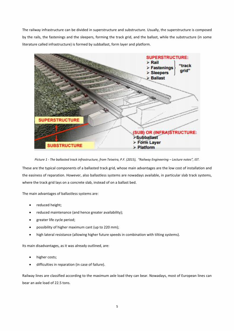
The railway infrastructure can be divided in superstructure and substructure. Usually, the superstructure is composed
by the rails, the fastenings and the sleepers, forming the track grid, and the ballast, while the substructure (in some
literature called infrastructure) is formed by subballast, form layer and platform.
Picture 1 - The ballasted track infrastructure, from Teixeira, P.F. (2015), “Railway Engineering – Lecture notes”, IST.
These are the typical components of a ballasted track grid, whose main advantages are the low cost of installation and
the easiness of reparation. However, also ballastless systems are nowadays available, in particular slab track systems,
where the track grid lays on a concrete slab, instead of on a ballast bed.
The main advantages of ballastless systems are:
reduced height;
reduced maintenance (and hence greater availability);
greater life cycle period;
possibility of higher maximum cant (up to 220 mm);
high lateral resistance (allowing higher future speeds in combination with tilting systems).
Its main disadvantages, as it was already outlined, are:
higher costs;
difficulties in reparation (in case of failure).
Railway lines are classified according to the maximum axle load they can bear. Nowadays, most of European lines can
bear an axle load of 22.5 tons.
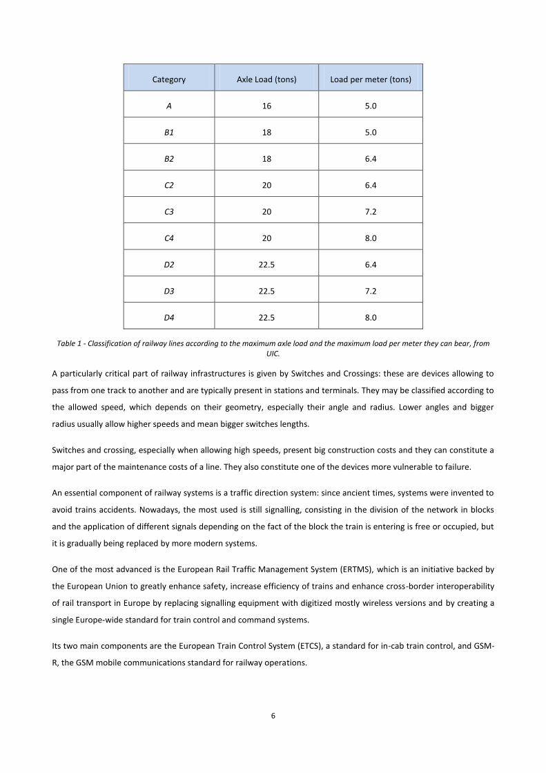
6
Category Axle Load (tons) Load per meter (tons)
A 16 5.0
B1 18 5.0
B2 18 6.4
C2 20 6.4
C3 20 7.2
C4 20 8.0
D2 22.5 6.4
D3 22.5 7.2
D4 22.5 8.0
Table 1 - Classification of railway lines according to the maximum axle load and the maximum load per meter they can bear, from UIC.
A particularly critical part of railway infrastructures is given by Switches and Crossings: these are devices allowing to
pass from one track to another and are typically present in stations and terminals. They may be classified according to
the allowed speed, which depends on their geometry, especially their angle and radius. Lower angles and bigger
radius usually allow higher speeds and mean bigger switches lengths.
Switches and crossing, especially when allowing high speeds, present big construction costs and they can constitute a
major part of the maintenance costs of a line. They also constitute one of the devices more vulnerable to failure.
An essential component of railway systems is a traffic direction system: since ancient times, systems were invented to
avoid trains accidents. Nowadays, the most used is still signalling, consisting in the division of the network in blocks
and the application of different signals depending on the fact of the block the train is entering is free or occupied, but
it is gradually being replaced by more modern systems.
One of the most advanced is the European Rail Traffic Management System (ERTMS), which is an initiative backed by
the European Union to greatly enhance safety, increase efficiency of trains and enhance cross-border interoperability
of rail transport in Europe by replacing signalling equipment with digitized mostly wireless versions and by creating a
single Europe-wide standard for train control and command systems.
Its two main components are the European Train Control System (ETCS), a standard for in-cab train control, and GSM-
R, the GSM mobile communications standard for railway operations.
7
Various levels of ERTMS can be applied. At level 1 signals still coexist with ERTMS balizes; at level 2 no signals are
present, the position of the train is just updated through balizes and all the information is transmitted through GSM-R,
but the network is still divided in blocks for traffic control purposes; level 3 differs from level 2 because the concept of
moving block is introduced, thus the exact position of the preceding train is known.
2.3 Current challenges for European Railways
Even though railway system might contribute greatly to the achieving of EU policy goals in the transportation field,
especially in terms of congestion reduction, oil dependency and green-house gases emissions, Rail transport in Europe
has been in decline in recent decades, especially in freight.
Rail’s share in the freight land transport market dropped from 32.6 % in 1970 (EU-15) to just 16.7 % in 2006 in the EU-
27. In absolute terms, based on the amount of goods carried and distances transported, rail freight transport activity
(EU-15) declined between 1970 and 2006 by about 1%. However, freight transport by road more than tripled in the
same period.
In terms of passenger transport, in 1970 (EU-15), rail’s share of passenger land transport was over 10% but this fell to
a 6.9% in 2006 in the EU-27, even though there was more rail travel in absolute terms.
This is due to the fact that rail does have certain weaknesses that it must overcome.
There is still a certain lack of dynamism, reliability, flexibility and customer orientation on the part of railway
undertakings. At times the political influence on the railway business is too strong, while there is still insufficient
interoperability between national rail systems as well as insufficient — and decreasing — investment.
In addition, rail is often hamstrung by outdated business and operational practices, by the presence of too much
ageing infrastructure and rolling stock and by a financial situation that is often weak.
The main consequences of EU rail weaknesses are:
the scarcity of capacity, meaning that the old technologies adopted in the infrastructures and rolling stock,
including the limitation of the axle load to 22.5 tons, and the sharing of the infrastructures between
passengers and freight fix a very low limit to capacity;
the lack of reliability, meaning that the possibilities of creating delays, especially in freight transport is rather
high, mainly due to the scarcity of capacity;
the low travel time competitiveness, due to many factors, including delays due to the scarce capacity and
interoperability issues when the service has to cross a border.
2.4 Possible answers to European Railways challenges
EU funded many projects concerning railway system during the last decades, in order to seek answers to the
challenges presented in the last paragraph.
8
Much work has been carried out with the aim of giving priority to some very important corridors. These corridors
constitute a network covering almost every corner of the territory of the continent and their importance is strategic.
Since July 1996, after a decision of EU parliament and council, this network has the name of TEN-T (Trans-European
Transport Network) and has been object of great EU funding. In the following, a paragraph is dedicated to a brief
description of what TEN-T actually is.
Many research projects focused on the development of new technologies have also been funded by EU.
Among the most important projects funded in the recent past we may find Eurobalt and Innotrack.
The Eurobalt project set as its goal to determine, model and understand which parameters in the train/track
interaction are primarily responsible for the serious degradation problems occurring especially when the track is
loaded with high speed or freight trains. Based on the experimental results, advanced parametric models were
subsequently proposed in order to optimize track design and maintenance. A set of concluding specifications has also
been proposed with the objective of aiding the future construction of tracks.
The INNOTRACK project is a joint response of the major stakeholders in the rail sector for the development of cost-
effective high-performance track infrastructure, aiming at providing innovative solutions towards significant
reductions in both investment and maintenance of infrastructure costs.
Today, a new major project is in progress, involving new technologies both on the infrastructure and on the vehicles
sides and its name is Capacity4Rail (C4R). As it is clear from the name, the project’s main objective is to find solutions
for the scarcity of available capacity, but many of the rail weaknesses previously described are considered. An entire
paragraph in the following of the text is dedicated to this project, which constitutes the framework in which the
present work has been developed.
2.4.1 Trans-European Transport Network (TEN-T)
The Trans-European Transport Networks (TEN-T) are a planned set of road, rail, air and water transport networks in
the European Union. They are part of a wider system of Trans-European Networks (TENs), including a
telecommunications network (eTEN) and a proposed energy network (TEN-E or Ten-Energy). The European
Commission adopted the first action plans on trans-European networks in 1990.
Trans-European transport network was planned in order to strengthen the social, economic and territorial cohesion of
the European Union.
As stated in article 4 of the Regulation (EU) 1315/2013 the aim is to create a single European transport area, which is
efficient and sustainable, to increase the benefits for its users and to support inclusive growth.
As referred in the same document, the Member States agreed to lists of corridor specific objectives, which have to be
met by the Corridor by 2030 the latest.
Regarding railways, seven main objectives are identified:
9
- implementation of the standard track gauge of 1435 mm;
- implementation of full electrification and the same electrification system;
- full implementation of ERTMS/ETCS;
- allow a train length of, at least, 740 m;
- allow an axle load of, at least, 22.5 tons;
- implementation of, at least, loading gauge P400 (for semitrailers);
- minimum speed of 100 km/h.
The compliance of specific corridors with the objectives is graphically represented in compliance maps, annexes to the
TEN-T core network reports.
For example, a map representing the compliance to the maximum train length objective in the Scandinavian
Mediterranean corridor, is presented in ANNEX 2.
In order to reach the referred objectives, projects are necessary.
Depending on the compliance of a certain corridor with the objectives, lists of projects were elaborated. Also these
lists are annexes to the reports.
2.4.2 Capacity4Rail (C4R) research project
2.4.2.1 Project overview
As mentioned earlier, the EC has put an important effort financing large scale research projects envolving the industry
main players, in order to foster the competitiveness of the railway system. Among those, the currently ongoing C4R
project envolving 48 partners (among which IST) and proposes to address a number of current limitations of European
railways.
As suggested by the project’s name, one of the main issues addressed is railway capacity.
C4R aims at paving the way for the future railway system, delivering coherent, demonstrated, innovative and
sustainable solutions.
The project is composed by many Work Packages (WP), grouped in 6 sub-projects (SP), devoted to infrastructure, new
concepts for efficient freight systems, operations for enhanced capacity, advanced monitoring, system assessment
and migration to 2030/2050 and management, dissemination, training & exploitation.
As it was already referred in chapter 1, the aim of the present work will be the building of a possible assessment tool
for the innovations introduced by C4R, however, before doing so, it seems good to explore which are the innovations
being developed by C4R project studies, in order to understand their possible performances and impacts.
The main technological innovations that will be developed regard:

10
- new track concepts;
- Switches and Crossings;
- novel freight wagons;
- upgrade of interchanges;
- advanced monitoring systems.
Each of these elements will be briefly described in the following paragraphs.
2.4.2.2 The introduced innovations
2.4.2.2.1 New track concepts
In WP1 new track concepts, based on the prefabricated slab track, will be developed.
The new track will be low maintenance due to advance maintainability because of health monitoring.
Environmental efficiency and LCC will also be taken into account: because of the use of recycled materials, it will also
be low carbon.
The resilience to natural hazard will also be considered an important aspect, mainly for extreme weather conditions,
including heavy rain and flooding.
Part of this task of the project is also the development of rapid construction techniques based on modular
construction.
2.4.2.2.2 Switches and Crossings
Nowadays, these devices constitute one of the components of the infrastructure responsible for the most failures and,
thus, maintenance costs and operational problems.
A new generation of Switches and Crossings will be developed through a deep study of failure modes.
Curving physics will also be taken into account, in order to improve curving, dynamics of running through switch and,
hence, lower material damage.
2.4.2.2.3 Novel freight wagons
SP 2 will develop the rail freight system of the future.
The design of the wagons will enhance its and the train capacity. In particular, trains with an axle load of 25 tons will
be foreseen.
Integrate couplers, mechanical and electronic connections and other means will permit longer trains.
Failure detection systems will also be developed.
11
2.4.2.2.4 Upgrade of interchanges
Novel technologies and operational measures (e.g. extended automation) are foreseen to be developed in order to
enhance the terminal performance and the behavior of the future terminal.
2.4.2.2.5 Advanced monitoring
The objective of SP4 is to develop new concepts for railways structural and operational monitoring to enhance the
availability of the track combined with automated maintenance forecasts, a prediction of the structural lifetime, a
fast-check of track and structures after natural hazards and a support for train operation by train monitoring.
2.4.2.3 The challenge of assessing the future impact of innovations
C4R is also aimed to answer the question “How to obtain an affordable, adaptable, automated, resilient and high-
capacity railway for 2020, 2030 and 2050?” and develop a ‘roadmap’ that paves the way for an affordable, automated,
resilient and high-capacity railway.
Due to the special character of the project, a big challenge is to provide adapted methods and tools for the
assessment of innovations, technologies and concepts, creating and assessing scenarios with the objective of
achieving European Transport Policy goals.
The present work is indeed aimed to elaborate a proposal of an assessment tool for the innovations introduced by
C4R, developed in partnership with the investigation team of IST in charge for C4R, and evaluate some basic scenarios
in order to take conclusions that could help to orientate about which is the most profitable combination of
innovations. The main goal is to understand if the new technologies have any impact and, then, if it is a positive or
negative impact and which combination of investments has the best impact.
Some of the questions we will try to answer with this work are: “Is it worth to invest?”, “Is it better to invest in the
application of all the innovations or just of a restricted group of them?”, “Is it better to invest just in the most
congested segments or in the whole network?”.
The following chapter will be dedicated to the revision of the state of art about assessment methodologies, in order to
establish which of them is the most suitable for this situation.
12
3. RAILWAY INVESTMENTS APPRAISAL
3.1 Investment appraisal tools to assess major investments
The main aim of economic evaluation of projects is to identify and quantify their contribution to the well-being of
society. Due to the lack of resources, which is always reflected by public administrations, together with the need for
investment decision, the Cost-Benefit Analysis (CBA) of public investments became a fundamental instrument of
projects evaluation.
CBA is defined as an analytical tool used to appraise an investment decision in order to assess the welfare change
attributable to it.
It has a role to play not just in ex ante evaluations, but also when the project is being executed (in medias res) or even
when it has already been finished (ex post). In these last two cases the aim is not to decide whether to execute the
project or not, but rather to assess if modifications are necessary, considered the new available information (in
medias res), or to draw important lessons that may improve the design of future projects (ex post).
European legislation requires a CBA as a basis for decision making in the appraisal of the so-called major projects,
being a major project an investment operation comprising “a series of works, activities or services intended to
accomplish an indivisible task of a precise economic and technical nature which has clearly identified goals and for
which the total eligible cost exceeds EUR 50 million” (Article 100 of Regulation (EU) No 1303/2013). In this definition,
the total eligible cost is the part of the investment cost which is eligible for EU co-financing.
However, CBA analysis presents some critical aspects. For example, distributional effects are usually not considered.
That is why CBA can be compensated by other types of analysis in the assessment of major investment: Multiple-
criteria decision analysis (MCDA) can be a valuable complementary tool to CBA.
3.2 Cost-Benefits Analysis according to EC guidelines
European Commission (EC) offers practical guidance on major projects appraisal through Guides to Cost-Benefit
Analysis of investment projects, the last of which was published in 2014 updating and expanding the previous version
of 2008.
According to EC guidelines, a standard CBA should be structured in seven steps:
1. Description of the context
2. Definition of objectives
3. Identification of the project
4. Technical feasibility and Environmental sustainability
5. Financial analysis
6. Economic analysis
13
7. Risk assessment.
The following paragraphs shall describe each of the indicated steps.
3.2.1 Description of the context
The first step of the project appraisal process involves a description of the social, economic, political and institutional
context in which the project is going to be implemented.
Context description is instrumental to forecast future trends, in particular demand trends.
This step is also useful to understand if the project is appropriate to the context in which it takes place.
The implementation of a project should always be justified and the reason to justify it should always base on the
diagnosis of an initial situation where possible improvements are detected: a project contributes to social well-being
insofar as the benefits generated by the resolution of an existing problem overcome the costs of the intervention. If
no problems exist, benefits could hardly be generated.
3.2.2 Definition of objectives
From the analysis of all the contextual elements listed in the previous section, the regional and/or sectorial needs that
can be addressed by the project must be assessed, in compliance with the sectorial strategy prepared by the Member
State and accepted by the European Commission. The project objectives should then be defined in explicit relation to
needs.
As far as possible, objectives should be quantified through indicators and targeted.
A clear definition of the project objectives is necessary to:
identify the effects of the project to be further evaluated in the CBA.
verify the project’s relevance.
A common mistake is to confuse project objectives with its outputs. For instance, if the main objective of the project is
to improve the accessibility of a peripheral area, the construction of a new road or the modernization of the existing
network are not objectives, but the means through which the objective of improving the area’s accessibility will be
accomplished.
Typical objectives for transport projects may be:
reduction of congestion within a network, link or node by resolving capacity constraints;
improvement of the capacity and/or performance of a network, link or node by increasing travel speeds and
by reducing operating costs and accidents;
improvement of the reliability and safety of a network, link or node;
14
minimization of GHG emissions, pollution and limitation of the environmental impact (important examples
are projects supporting the shift from individual, i.e. cars, to collective transport);
adjustment to EU standards and completion of missing links or poorly linked networks: transport networks
have often been created on a national and/or regional basis, which may no longer meet the transport
requirements of the single market (this is mainly the case with railways);
improvement of accessibility in peripheral areas or regions.
3.2.3 Project identification
A transport project is an intervention over a transport market able to modify the equilibrium that would be obtained
in this market and in the rest of economy if the intervention would not be carried out.
Its evaluation will consist in the comparison between different equilibrium conditions. Through this comparison, the
impacts of the project on society may be determined.
According to EC 2014 Guide to Cost-benefit Analysis of Investment Projects, a project is considered clearly identified
when:
the physical elements and the activities that will be implemented to provide a given good or service, and to
achieve a well-defined set of objectives, consist of a self-sufficient unit of analysis;
the body responsible for implementation (often referred to as ʻprojectpromoterʼ or ʻbeneficiaryʼ) is identified
and its technical, financial and institutional capacities analyzed; and
the impact area, the final beneficiaries and all relevant stakeholders are duly identified (ʻwho has standing?ʼ).
The first condition means that the project must include all the elements necessary for its working and exclude all the
elements that are projects perfectly separable and separately evaluable. The exclusion of components that are
necessary from the project definition may increase fictitiously the project profitability, while the inclusion of separable
projects may lead to an average profitability hiding the profitability of every single project individually considered.
About the identification of the project owner of promoter, his technical, financial and institutional capacities must be
described. The technical capacity refers to the relevant staff resources and staff expertise available within the
organization of the project promoter and allocated to the project to manage its implementation and subsequent
operation. The financial capacity refers to the financial standing of the body, which should demonstrate that it is able
to guarantee adequate funding both during implementation and operations. The institutional capacity refers to all the
institutional arrangements needed to implement and operate the project, including the legal and contractual issues
for project licensing. When the operator is different from the owner, a brief description of the operating company
should be added.
The third element necessary for the definition of a project is the answer to the questions ʻwho has standing?ʼ. Even
though the definition of the bodies affected by the project may depend on the level of aggregation and vary between
the projects, the following list of agents should at least be taken into account:
15
transport infrastructures and services users, including both the direct consumers of transport services and
infrastructures and the owners of the freight consuming them. They may be individuals, social groups or even
companies;
transport infrastructures and services producers: usually they are public or private companies making
available services or infrastructures, but in the case of own-account operations, producers and users
coincide. When the evaluation requires it, the producers could be divided into owners of the assets, of the
work and of the lands;
tax-payers, to be included when the project involves modifications of taxes and subsidies;
the rest of society, affected by not internalized external effects.
The effects of the project may not be limited to the primary transport market (the one where the intervention is
realized), but they often have implications on other markets related to the primary (secondary markets) and on the
global economic activity (additional economic effects).
The impact on the primary market are usually defined as direct effects, while the impact on the secondary market are
referred to as indirect effect.
About the indirect effects, they may be disregarded if no significant distortions affecting the free interaction between
offer and demand are present in the market.
Thus far, there are no models available for the study of the additional economic effects, that are mainly related to
factors like economies of scale or agglomeration economies, or to the long-term reaction of the social agents to the
improvements introduced in the transport system. In small projects, it is considered advisable to disregard completely
these effects, while more sophisticated macroeconomic analysis are justified for big projects.
It is remarkable that effects deriving from the improvement of transport services on markets of products using these
services as an input must be ignored. This is not due to a disregarding choice, but to the fact that the benefits of the
reduction of the cost of transport will have already been evaluated in the primary market and the evaluation of those
effects would consists in a case of double-counting.
The evaluator must be constantly worried about avoiding double-counting.
3.2.4 Technical feasibility and environmental sustainability
Although these analyses are not formally part of the CBA, their results should be briefly reported and used as data
source for the CBA.
According to EU CBA guidelines, detailed information should be provided on:
demand analysis;
options analysis;
environment and climate change considerations;
16
technical design, cost estimates and implementation schedule.
The demand analysis should identify both the current demand (based on statistics provided by service operators or
national or local government) and the future demand (based on reliable forecasting models).
For every problem an adequate range of options should be provided. The diversity of the alternatives depends on the
level of discretion left to the evaluator. For example, if he deals with the construction of a certain motorway, most
alternatives will be related to the path or the constructive processes, while, if more discretion is given to the
evaluator, for example instructing him to solve the problem of the connection between two cities, the alternatives
range will be wider, including, besides the motorway, other transport mode solutions.
In the elaboration of the alternatives, particular care should be put in the role assigned to technology: sometimes,
adequate maintenance or small improvements of the existing technology have a larger impact on social well-being
than the most technologically advanced option.
However, disregarding viable alternatives may lead to great mistakes.
CBA is always carried out in an incremental approach, meaning by comparison of every solution (with-project
situation) with the so-called counterfactual scenario (without-project situation) evaluating their differences in benefits
and costs. The counterfactual scenario is then a special option representing which would have been the evolution of
the markets where the investment is realized, if it had not been realized at all.
Depending on the type of project and the available information, the counterfactual scenario might be given by a “Do-
minimum” scenario, where very small modifications are assumed to be realized or by a “Do-nothing” scenario or
“Business As Usual” (BAU). Even in this case, the without-project scenario does not consist in considering conditions to
be kept constant, but a future projection of the present equilibrium is considered, with possible changes in demand
and offer.
Environmental sustainability of the project should also be evaluated. When appropriate, an Environmental Impact
assessment (EIA) must be carried out to identify, describe and assess the direct and indirect effects of the project on
human beings and the environment. While the EIA is a formally distinct and self-standing procedure, its outcomes
need to be integrated in the CBA and be in the balance when choosing the final project option.
Impacts of the project on climate, in terms of reduction of GHG emissions, are referred to as climate change
mitigation and must be included in the EIA.
To conclude this chapter of the analysis, a summary of the proposed solutions should be presented, including the
following information: location, technical design, production plan, cost estimates, implementation timing.
17
3.2.5 Financial analysis
We get to the core of CBA analysis, where projects are evaluated in monetary terms. The difference between Financial
and Economic analysis is mainly related with the point of view from which they are carried out and the consequences
that this fact has.
While Economic analysis is usually carried out from the point of view of society, so it must include all the social costs
and benefits of all the stakeholders affected by the project, Financial analysis should generally be carried out from the
point of view of the infrastructure owner, then it just considers cash outflows and inflows.
In the majority of the projects analyzed with a CBA procedure, costs and benefits do not coincide with cash outflows
and inflows, that is why Financial and Economic analysis are two separate processes, even though they are related. It
is usual to start from the Financial analysis and then pass to the Economic one, basing on it.
The financial analysis should be based on the Discounted Cash Flow (DCF) method: project cash inflows and outflows
are estimated and displayed for every year during a time period called time horizon (or reference period), which
depends on the project's economically useful life and long term impacts.
The cash flows are usually expressed in constant (real) prices i.e. with prices fixed at a base-year. The use of current
(nominal) prices (i.e. prices adjusted by the Consumer Price Index (CPI)) would involve a forecast of CPI that does not
seem always necessary.
The analysis should be carried out net of Value Added Tax (VAT) both on costs and revenues, when it is recoverable by
the project promoter. Otherwise, it must be included. Direct taxes (on capital, income or other) are not considered for
the calculation of the financial profitability, which is calculated before such tax deductions. The rationale is to avoid
capital income tax rules complexity and variability across time and countries.
Clearly, during the first years, outflows will usually overcome inflows (construction period), while later the opposite
situation will be faced (operation period).
Through this method, a cash flow will be produced for every alternative. The matter is then to establish ways to
compare them. Even though many flows comparison tools exist, the most used in CBA field is the Financial Net
Present Value (FNPV), defined as the sum that results when the discounted values of the expected investment and
operating costs of the project are deducted from the discounted value of the expected revenues:
𝐹𝑁𝑃𝑉 = ∑𝑆𝑡
(1+𝑖)𝑡𝑛𝑡=0 =
𝑆0
(1+𝑖)0+
𝑆1
(1+𝑖)1+ ⋯ +
𝑆𝑛
(1+𝑖)𝑛, ( 1 )
where:
𝑡 indicates the year;
𝑖 is the Discount Flow Rate (DFR);
𝑆t is the sum resulting when the discounted values of the expected investment and operating costs of the
project in year 𝑡 are deducted from the discounted value of the expected revenues in year 𝑡.
18
The concept of flows discounting is fundamental both in FA and EA. This operation leads to the calculation of the
present value of future flows. Actually, it is not mandatory to consider the present value of the flows, because it is
possible to consider their value in another reference moment of the future, however it is common to calculate the
value of the flows at the moment of the beginning of the reference period.
This operation is based on the adoption of an appropriate Discount Flow Rate (DFR). About this rate, the European
Commission recommends a value of 4 % as the reference parameter for the programming period 2014-2020.
Even though the NPV is the most used indicator of financial profitability, it is not the only one. In fact, the Financial
Rate of Return (FRR) on investment is also considered a key indicator.
These two indicators are related: a negative FNPV implies a FRR lower than the applied DFR, which means that the
generated inflows do not cover the outflows and the project needs public investment assistance. On contrary, a
positive FNPV is associated with a FRR greater than the applied DFR.
3.2.5.1 Flows identification
Let us now focus on the identification of every possible item of the inflows and outflows list of a certain project. The
main focus will be on transport projects as they are the object of the analysis presented in the following chapter.
3.2.5.1.1 Investment costs
The first big group of outflows is given by the investment costs. Traditionally, they can deal with three different
processes: they may be construction costs of a new infrastructure, may be associated with the rehabilitation or the
modification of an existing infrastructure or may pay the purchase of assets needed for the implementation of new
services or for the modification of the existing ones.
In particular, when the construction of new infrastructures is involved, four sub-categories of investments costs can be
distinguished:
Planning costs, associated with technical and economical studies prior to the project start.
Costs of purchase and preparation of the lands.
Real construction costs.
Interruption costs, associated with the alterations suffered by transport users and the rest of society during
the construction.
Empirical evidence showed statistically that the majority of the projects incur in extra-costs.
3.2.5.1.2 Residual value
When the economic life of a given asset or infrastructure just coincides with the time horizon of the analysis, at the
end of this period it does not have any value and no further calculation are needed. However, this happens rather
19
rarely and, in the majority of transport projects, the economic life of the assets is greater than the evaluation
reference period: that is why the concept of Residual Value (RV) must be introduced.
The RV is a measure of the value that the assets or the infrastructure still have after the end of the time horizon of the
analysis.
Since it corresponds to a moment far away in time and many variables may have influence on it, much uncertainty
remains concerning its determination. Two main methods are available:
Getting the RV basing on the initial investment. The value of the RV is just a function, usually a simple
percentage, of the initial investment. This method has the clear advantage of being very simple, but the fact
that the RV does not have any relation with the project inflows and outflows is a big disadvantage.
Getting the RV from the NPV of inflows and outflows subsequent to the evaluation horizon. This method
presents a greater consistency compared to the previous one, though it requires a greater computational
effort.
3.2.5.1.3 Operating and maintenance (O&M)
Before characterizing these parts of the outflows, it should be specified that not always do all of them be considered
in the FA. This is related to the adopted point of view and to the role of the personality whose point of view is
considered. For example, if the considered point of view is the owner's and he is not in charge for transport
operations, just infrastructure maintenance outflows will be considered. However, in the most general case, the
owner of the infrastructure is also in charge for the operation and both of the outflows component have to be
considered.
The Maintenance outflows are the ones that guarantee that the infrastructures, the vehicles and the rest of the assets
remain in adequate conditions during all the reference period of the analysis.
Operating outflows are, instead, related to the usual operation of infrastructures, vehicles and other assets.
Even though both these items of outflows may have a fixed portion, part of them is usually variable and proportional
to the traffic demand.
Both these costs components share the characteristic of being spread all over the life of the project, unlike the
investment costs, which are usually concentrated mainly in the first period.
It could be useful to classify both Maintenance and Operating flows according to their origin:
Costs related to vehicles or assets in general. They include mainly maintenance and reparations. Annual fall in
price must not be included here, because the entire costs of vehicles and other assets was taken into account
when the initial investment was considered.
Costs related to using time, where the main component is usually given by the personnel for service to
passengers and freight.
20
Costs related to travelled distance, where the main component is usually fuel.
3.2.5.1.4 Revenues
The project revenues are defined as the “cash in-flows directly paid by users for the goods or services provided by the
operation, such as charges borne directly by users for the use of infrastructure, sale or rent of land or buildings, or
payments for services” (Article 61 (Operations generating net revenue after completion) of (EU) Regulation
1303/2013).
These revenues will be determined by the quantities forecasts of goods/services provided and by their prices.
Incremental revenues may come from increases in quantities sold, in the level of prices, or both.
For compliance with the regulatory requirements, where relevant tariffs shall be fixed in compliance with the polluter-
pays and the full-cost recovery principles.
3.2.6 Economic analysis
This can be considered the most important part of CBA: in this phase the project's contribution to the welfare is
evaluated through the analysis of its costs and benefits. Due to its importance, more attention will be dedicated to
this step in the following part of the text.
A key concept of EA is the use of shadow prices reflecting the real social opportunity cost of goods and services
instead of their market prices, which may suffer distortion.
When a PA takes the decision to allocate funds for the execution of a certain project, it renounces at the same time to
the benefits that could be got if the same funds would have been allocated for other purposes. When a choice needs
to be made between several mutually exclusive alternatives, the opportunity cost of a project is given by the benefits
that society might obtain from the best alternative forgone.
Dealing with shadow prices is not as straightforward as dealing with simple monetary outflows. Some of the items
that will be considered have a market and, in these cases, the determination of shadow prices is simpler, because it
can consist just in correcting their market prices with a factor. However, some of the items considered do not have
any market and their market prices have to be determined with a project-specific study or, for minor project that do
not justify it, basing on existing studies.
About the goods for which a market exists, market prices could be a good approximation of their shadow prices
whenever the market is not affected by notable distortions. Possible sources of market distortions (or market failures)
are manifold:
non-efficient markets where the public sector and/or operators exercise their power (e.g. subsidies for
energy generation from renewable sources, prices including a mark-up over the marginal cost in the case of
monopoly, etc.);
21
administered tariffs for utilities may fail to reflect the opportunity cost of inputs due to affordability and
equity reasons;
some prices include fiscal requirements (e.g. duties on import, excises, VAT and other indirect taxes, income
taxation on wages, etc.);
for some effects no market (and prices) are available (e.g. reduction of air pollution, time savings).
The standard approach to EA is to move from Financial to Economic Analysis. Firstly, the following adjustments should
be made:
fiscal corrections;
conversion from market to shadow prices;
evaluation of non-market impacts and correction for externalities.
After these adjustments, costs and benefits occurring at different times should be discounted. The discount rate in the
economic analysis of investment projects, the Social Discount Rate (SDR), reflects the social view on how future
benefits and costs should be valued against present ones. For the programming period 2014-2020, the European
Commission recommends that for the social discount rate 5 % is used for major projects in Cohesion countries and 3 %
for the other Member States.
After the use of the appropriate SDR, it is possible to calculate the project economic performance measured by the
following indicators: Economic Net Present Value (ENPV), Economic Rate of Return (ERR) and benefit/cost ratio (B/C
ratio).
3.2.7 Risk assessment
A risk assessment should always be included in the CBA, in order to deal with the uncertainty that is always associated
to investment project, included climate change. The steps recommended to carry out a risk assessment procedure are:
sensitivity analysis;
qualitative risk analysis;
probabilistic risk analysis;
risk prevention and mitigation.
3.2.7.1 Sensitivity analysis
This analysis allows the identification of the “critical variables” of the project, which are the variables whose variations
have the largest impact on the project’s financial and/or economic performance. The analysis is carried out varying
one variable at a time and determining the effect of that change on the NPV. The recommendation is to consider
critical those variables for which a variation of ± 1% of the value adopted in the base case gives rise to a variation
greater than 1% in the final value of NPV.
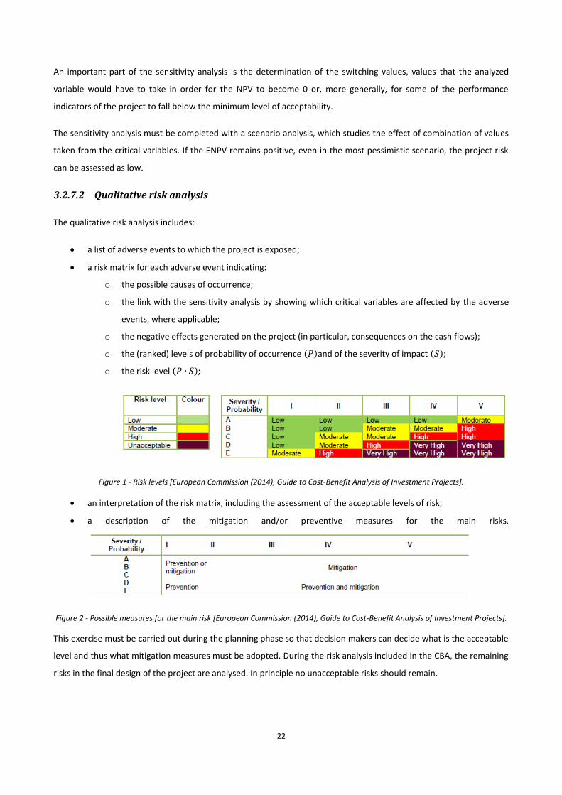
22
An important part of the sensitivity analysis is the determination of the switching values, values that the analyzed
variable would have to take in order for the NPV to become 0 or, more generally, for some of the performance
indicators of the project to fall below the minimum level of acceptability.
The sensitivity analysis must be completed with a scenario analysis, which studies the effect of combination of values
taken from the critical variables. If the ENPV remains positive, even in the most pessimistic scenario, the project risk
can be assessed as low.
3.2.7.2 Qualitative risk analysis
The qualitative risk analysis includes:
a list of adverse events to which the project is exposed;
a risk matrix for each adverse event indicating:
o the possible causes of occurrence;
o the link with the sensitivity analysis by showing which critical variables are affected by the adverse
events, where applicable;
o the negative effects generated on the project (in particular, consequences on the cash flows);
o the (ranked) levels of probability of occurrence (𝑃)and of the severity of impact (𝑆);
o the risk level (𝑃 ∙ 𝑆);
Figure 1 - Risk levels [European Commission (2014), Guide to Cost-Benefit Analysis of Investment Projects].
an interpretation of the risk matrix, including the assessment of the acceptable levels of risk;
a description of the mitigation and/or preventive measures for the main risks.
Figure 2 - Possible measures for the main risk [European Commission (2014), Guide to Cost-Benefit Analysis of Investment Projects].
This exercise must be carried out during the planning phase so that decision makers can decide what is the acceptable
level and thus what mitigation measures must be adopted. During the risk analysis included in the CBA, the remaining
risks in the final design of the project are analysed. In principle no unacceptable risks should remain.
23
For each adverse event, it is suggested to assess the residual risk after the implementation of the measures. If risk
exposure is assessed to be acceptable (i.e. there are no longer high or very high risk levels), the proposed qualitative
risk strategy can be adopted. If a substantial risk remains, it is required to move to a probabilistic quantitative analysis
to further investigate the project risks.
3.2.7.3 Probabilistic risk analysis
This analysis is required where the residual risk exposure is still significant. In other cases, it may be carried out where
appropriate, depending on project size and data availability.
It consists in assigning a probability distribution to each of the critical variables figured out in the sensitivity analysis in
order to calculate the expected values of the financial and economic performance indicators.
Once established the probability distributions of the critical variables, it is possible to proceed to the calculation of the
probability distribution of the FRR or the ENPV of the project. It is suggested the use of Monte Carlo method,
consisting in repeated random extractions of a set of values for the critical variables, taken within the respective
defined intervals.
Then, the performance indices for the project (FRR, ENPV or others) are calculated from each set of extracted
variables.
The values obtained enable the analyst to infer significant judgments about the level of risk of the project.
3.2.7.4 Risk prevention and mitigation
Risk assessment should be the basis for risk management, which is the identification of strategies to reduce risks,
including how to allocate them to the parties involved and which risks to transfer to professional risk management
institutions such as insurance companies. Risk management is a complex task and it can be considered as a role for
professionals, under the responsibility of the managing authority and the beneficiary.
The project promoter should, however, following the risk assessment, at least identify specific measures (including
responsibilities for their application) for the mitigation and/or prevention of the identified risks, according to
international good practice.
3.3 Focus on Economic Analysis
3.3.1 Introduction
As it was already referred, the standard approach to EA is to move from Financial to Economic Analysis. Firstly, the
following adjustments should be made:
fiscal corrections;
conversion from market to shadow prices;

24
evaluation of non-market impacts and correction for externalities.
After these adjustments, costs and benefits occurring at different times should be discounted. Then, it is possible to
calculate the project economic performance measured by the following indicators: Economic Net Present Value
(ENPV), Economic Rate of Return (ERR) and benefit/cost ratio (B/C ratio).
3.3.1.1 Fiscal correction
Taxes and subsidies are transfer payments that do not represent real economic costs or benefits for society as they
involve merely a transfer of control over certain resources from one group in society to another. Some general rules
can be established to correct such distortions:
prices for input and output must be considered net of VAT;
prices for input should be considered net of direct and indirect taxes;
prices (e.g. tariffs) used as a proxy for the value of outputs should be considered net of any subsidy and other
transfer granted by a public entity.
3.3.1.2 Conversion from market to shadow prices
As it was already referred, when market prices do not reflect the opportunity cost of inputs and outputs, the usual
approach is to convert them into shadow prices to be applied to the items of the financial analysis. To do so, the
following operational approach could be applied.
For project inputs:
If they are tradable goods, border prices are used. If a project uses an imported input, e.g. gas and oil, the
shadow price is the import cost plus insurance and freight in more liberalized (i.e. competitive and
undistorted) markets, thus excluding any custom duties or taxes applied once the good enters the national
market.
If they are non-tradable goods:
Standard Conversion Factors are used;
ad Hoc assumptions are made;
for manpower, shadow wage is calculated. Typically, in an economy characterized by extensive
unemployment or underemployment, this may be less than the actual wage rates paid.
For project outputs:
Users’ marginal Willingness-To-Pay (WTP), which measures the maximum amount consumers are willing to
pay for a unit of a given good, is used to estimate the direct benefit(s) related to the use of the goods or
services rendered by the project.
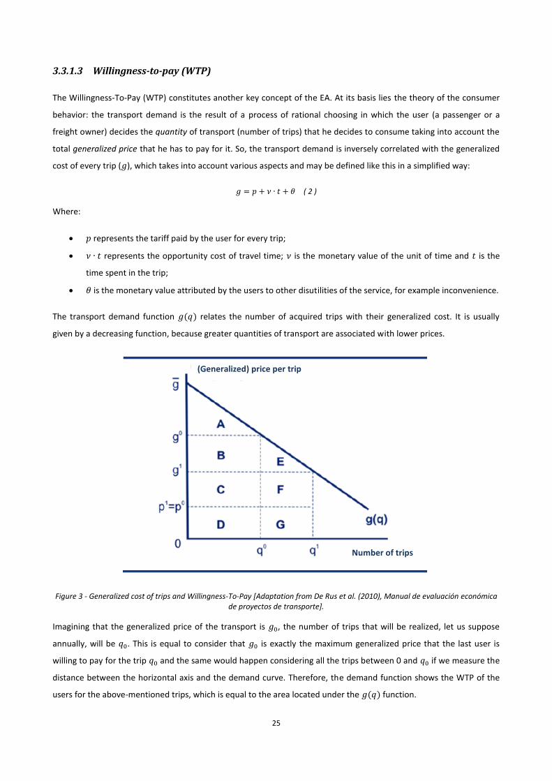
25
3.3.1.3 Willingness-to-pay (WTP)
The Willingness-To-Pay (WTP) constitutes another key concept of the EA. At its basis lies the theory of the consumer
behavior: the transport demand is the result of a process of rational choosing in which the user (a passenger or a
freight owner) decides the quantity of transport (number of trips) that he decides to consume taking into account the
total generalized price that he has to pay for it. So, the transport demand is inversely correlated with the generalized
cost of every trip (𝑔), which takes into account various aspects and may be defined like this in a simplified way:
𝑔 = 𝑝 + 𝜈 ∙ 𝑡 + 𝜃 ( 2 )
Where:
𝑝 represents the tariff paid by the user for every trip;
𝜈 ∙ 𝑡 represents the opportunity cost of travel time; 𝜈 is the monetary value of the unit of time and 𝑡 is the
time spent in the trip;
𝜃 is the monetary value attributed by the users to other disutilities of the service, for example inconvenience.
The transport demand function 𝑔(𝑞) relates the number of acquired trips with their generalized cost. It is usually
given by a decreasing function, because greater quantities of transport are associated with lower prices.
Figure 3 - Generalized cost of trips and Willingness-To-Pay [Adaptation from De Rus et al. (2010), Manual de evaluación económica de proyectos de transporte].
Imagining that the generalized price of the transport is 𝑔0, the number of trips that will be realized, let us suppose
annually, will be 𝑞0. This is equal to consider that 𝑔0 is exactly the maximum generalized price that the last user is
willing to pay for the trip 𝑞0 and the same would happen considering all the trips between 0 and 𝑞0 if we measure the
distance between the horizontal axis and the demand curve. Therefore, the demand function shows the WTP of the
users for the above-mentioned trips, which is equal to the area located under the 𝑔(𝑞) function.
(Generalized) price per trip
Number of trips
26
Of course, in this type of model, a decrease in the generalized costs of the transport would lead to an increase of the
number of trips.
Different techniques, including revealed preference and stated preference, exist to empirically estimate the demand
curve.
3.3.1.4 Evaluation of non-market impacts and externalities
In this part of the CBA, winners and losers are established, i.e. the positive and negative impacts of the project on
every agent identified in paragraph 3.2.3 are evaluated.
The impacts can be divided into four major groups:
variation of consumer surplus;
variation of producer surplus;
variation of tax-payers surplus;
variation of rest of society surplus.
In the evaluation the objective is not to seek the total surplus, but the variation it experiences as a consequence of the
project.
3.3.1.4.1 Consumer surplus
The variation of the consumer surplus is a monetary measure of the improvement of the well-being of this group of
agents and it is related with the concept of WTP which was presented in paragraph 3.3.1.3. Formally, the consumer
surplus is defined as the difference between the total value that the users attribute to the transport quantity they are
acquiring and the generalized price they pay for it.
Considering again the graph in paragraph 3.3.1.3, imagining that (𝑔0, 𝑞0) is the initial equilibrium condition, in this
state the consumer surplus is given just by A area, i.e.:
𝐶𝑆0 =1
2∙ (�̅� − 𝑔0) ∙ 𝑞0, ( 3 )
whilst in the new equilibrium condition established after the project implementation (𝑔1, 𝑞1), the consumer surplus is
given by the sum of areas A+B+E:
𝐶𝑆1 =1
2∙ (�̅� − 𝑔1) ∙ 𝑞1. ( 4 )
Since the objective is not to look for the total surplus, but just its variation passing from the initial condition to the
new one, the consumer surplus to be considered is just B+E, that is the difference between the two previous
expressions. This surplus has two components: the effect of the reduction of the generalized costs (area B) and the
surplus of the new users who join the analyzed transport market (area E).
27
In order to calculate the consumer surplus, we should start from the consideration that the main changes that are
going to be considered are related to the time savings obtained by existing and diverted users and with the WTP of
new users.
First of all, comparing the with-project situation with the without-project one, existing and induced traffic should be
determined and the induced one should also be divided into diverted and generated traffic:
existing traffic is given by those users that were already part of the analyzed transport market and would
have continued there even without the project realization;
diverted traffic is formed by those users that leave another infrastructure or transport mode to take
advantage of the generalized price reduction in the primary market as a consequence of the improvements
introduced by the project implementation;
generated traffic is the one that would not exist in absence of the project and may be given by the same
users that increase the number of trips or by new users whose marginal benefit from realizing the trip was
smaller than the without project generalized price.
Time savings are multiplied directly for the number of users of existing and deviated traffic, while, for the generated
traffic, just half of the time saving is considered for the benefit calculation in order to consider the fact that users in
this category have different WTP. This convention is known as “Rule of Half”.
Of course, the calculation of time savings is subordinated to capacity problems.
Also tariff changes must be considered for the determination of the Users’ surplus.
Improvements of the quality of the existing services, especially the ones related with services comfort and reliability,
may constitute other possible benefits to be considered for the evaluation of users’ surplus. However, they are often
disregarded due to the difficulty of their determination, mainly related to the fact that they are not market goods and
no many studies have been carried out about their possible monetary values.
When passing to the matter of attaching a money value to the obtained benefits, many ways could be followed.
For example, for the monetization of time savings, the main options are:
a specific study for the users of the particular case under consideration could be carried out. This always
constitutes the best option, provided that financial and time resources enough are available;
when the previous option is not viable, it is advisable to adopt recommended values at national or
international level for transport project social evaluation;
if no recommended values exist, it is possible to use data from other studies or similar countries, considering
the proper adaptations.
The value of time usually grows with time; the most frequent way to model its growth is to assume a growing rate
equal to the GDP per capita, although some studies recommend to consider an elasticity between 0.7 and 1.
28
In the absence of specific studies and national recommended values, the values collected in the European project
HEATCO constitute, thus far, the widest and most recent collection of reference values.
3.3.1.4.2 Producer surplus
The producer surplus is the difference between the total income and the total variable costs of all the companies
(either public or private) participating in the construction and exploitation of the transport infrastructures and services
considered. Double counting of costs and benefits must be strictly avoided, so, if a FA from the point of view of an
owner who is also a service operator has been performed, no other producer surplus has to be considered. However,
if owner and service operator are different, the FA should be carried out from the point of view of the owner, whilst in
this part of the analysis the service operator surplus should be considered.
Simplifying considering just one operator, the producer surplus is given by the following expression.
𝑃𝑆 = 𝑝 ∙ 𝑞 − 𝐶, ( 5 )
where:
𝑝 is the tariff users pay in exchange for the service;
𝑞 is the quantity of service acquired by the users;
𝐶 is the total cost for the producer, given mainly by operation costs.
The difference in PS between the situations with or without the project, ∆𝑃𝑆 = 𝑃𝑆1 − 𝑃𝑆0, can be calculated with the
following expression.
∆𝑃𝑆 = (𝑝1 ∙ 𝑞1 − 𝑝0 ∙ 𝑞0) − (𝐶1 − 𝐶0), ( 6 )
its sign and quantity depending on the way the project conditions income and costs of the companies.
As it was referred in the paragraph about FA, operating costs are related to the usual operation of vehicles and other
assets.
A part of them is usually variable and proportional to the traffic demand.
It could be useful to classify both them according to their origin:
Costs related to vehicles or assets in general. They include mainly maintenance and reparations. Annual fall in
price must not be included here, because the entire costs of vehicles and other assets was taken into account
when the initial investment was considered.
Costs related to using time, where the main component is usually given by the personnel for service to
passengers and freight.
Costs related to travelled distance, where the main component is usually fuel.
In order to monetize these costs, when specific information about the evaluated case is available, this is the base that
should be use. Otherwise, reference values and formulas should be sought. For the road traffic case many studies and,
29
consequently, reference values and formulas are available, while for the other transport modes the availability is
smaller.
3.3.1.4.3 Tax-payers surplus
Tax-payers surplus is given by the difference between the income they get by tax revenues and the expenditures due
to subsidies. If we simplify, admitting that those tax revenues and subsidies can be expressed through a unitary net
value of tax revenues per trip denoted by 𝜁, the variation of tax-payers surplus (Δ𝑇𝑃𝑆) is simply given by the
following expression.
𝛥𝑇𝑃𝑆 = 𝜁1 ∙ 𝑞1 − 𝜁0 ∙ 𝑞0, ( 7 )
where 𝜁 ∙ 𝑞 represents the tax-revenues, net of subsidies.
3.3.1.4.4 Rest of society surplus
The impacts being part of this group of effects of the project are also referred to as “externalities”, because they
affect agents that are external to the analyzed transport market (e.g. pollution and noise suffered by people that do
not use the mean of transport causing them) .
Taking into account that the majority of externalities in transport projects are costs, we can determine the variation of
the rest of society surplus (Δ𝑅𝑆𝑆) defining externalities as a unitary cost per trip (E):
(𝛥𝑅𝑆𝑆) = −(𝐸1 ∙ 𝑞1 − 𝐸0 ∙ 𝑞0). ( 8 )
This formula is actually a big simplification, because externalities are actually many and the determination of their
effects is not always so straight-forward.
The most evident externalities are atmospheric pollution (both local and global, like the Green House effect),
produced by all types of vehicles burning fuel, and noise. However, they are not the only possible externalities.
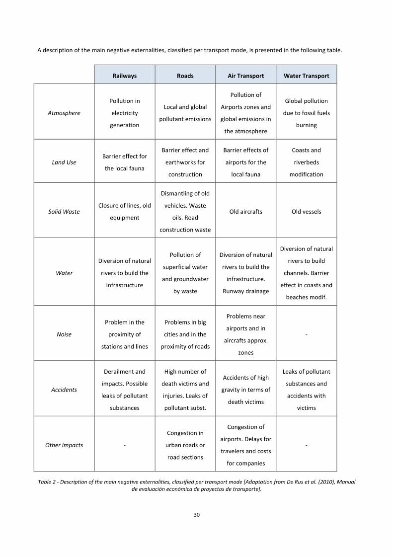
30
A description of the main negative externalities, classified per transport mode, is presented in the following table.
Railways Roads Air Transport Water Transport
Atmosphere
Pollution in
electricity
generation
Local and global
pollutant emissions
Pollution of
Airports zones and
global emissions in
the atmosphere
Global pollution
due to fossil fuels
burning
Land Use Barrier effect for
the local fauna
Barrier effect and
earthworks for
construction
Barrier effects of
airports for the
local fauna
Coasts and
riverbeds
modification
Solid Waste Closure of lines, old
equipment
Dismantling of old
vehicles. Waste
oils. Road
construction waste
Old aircrafts Old vessels
Water
Diversion of natural
rivers to build the
infrastructure
Pollution of
superficial water
and groundwater
by waste
Diversion of natural
rivers to build the
infrastructure.
Runway drainage
Diversion of natural
rivers to build
channels. Barrier
effect in coasts and
beaches modif.
Noise
Problem in the
proximity of
stations and lines
Problems in big
cities and in the
proximity of roads
Problems near
airports and in
aircrafts approx.
zones
-
Accidents
Derailment and
impacts. Possible
leaks of pollutant
substances
High number of
death victims and
injuries. Leaks of
pollutant subst.
Accidents of high
gravity in terms of
death victims
Leaks of pollutant
substances and
accidents with
victims
Other impacts -
Congestion in
urban roads or
road sections
Congestion of
airports. Delays for
travelers and costs
for companies
-
Table 2 - Description of the main negative externalities, classified per transport mode [Adaptation from De Rus et al. (2010), Manual de evaluación económica de proyectos de transporte].
31
Other externalities can be considered
landscape alteration: it affects almost all the infrastructures and implies loss of recreational and aesthetic
value;
vibrations: mainly coming from railways and air transport, they can interfere with some productive or
consume activities;
climate change: Green House Gases (GHG), mainly represented by CO2, included in the emissions of
transport, have global long-term effects that are more complex to quantify.
One way to firstly identify and then evaluate externalities to be considered in CBA is through dose-response functions.
In terms of the analysis, the transport activity would constitute the dose, while the response would be the
environmental impact, that has then to be evaluated to obtain the externality.
About the ways to attach a money value to the quantified externalities, different paths have to be followed according
to the type of externality considered.
For noise a study involving several European countries was realized recently (Navrud et al., 2006) and it includes the
calculation by a declared preferences method of the average amount of money that people are willing to pay per year
in order to eliminate the discomfort caused by noise produced by road or rail transport. Other studies contain possible
reference values for this type of externality: (Van den Berg at al.,2003 and Bickel at al., 2003).
About air pollution, besides its impact on life quality and human health, including morbidity or even death, has other
effects, as smaller visibility, deterioration of materials (buildings, statues, etc.) or climate effects. The most advisable
approach is a specific study on the evaluated case. The inconvenient of using other studies results is mainly related
with the fact that impacts are strongly dependent on the place and project studied. In lack of the possibility of a
specific study, HEATCO values could be adopted.
Landscape externalities constitute an impact which is extremely related to the place where the project is going to be
realized, so no reference values can be established and a study of every case is necessary.
Soil pollution may have effect over flora and fauna, agricultural productivity and, even, human health. For some of
these impacts, market prices could be used, while, for effects on human health, declared or revealed preference
method could be used.
Water pollution may have many different effects that can even be felt only later and be not circumscribed to the zone
where the pollution point is. No reference money values can be established, but every single case should be evaluated
on its own. Marin and fluvial fauna (including fishing production), the corresponding ecosystems, agricultural
production, recreational value of natural spaces, human health can all be affected.
Transport projects impacts on climate change are mainly related to emissions of GHG, like Carbon Dioxide (CO2),
methane (CH4) or nitrous oxide (N2O). These impacts are usually global long-term effects of rather different natures.
Many studies quantify the values to attribute to GHG emissions. These values are usually not defined for single
32
countries, due to the global impact of the emission, and they are considered to be growing in time. One more time, in
lack of better sources, it is advisable to use HEATCO values for tons of CO2 equivalent emissions.
Vibrations impacts can be divided into two groups:
discomfort to the listeners situated in the influence area: this impact may be included in the noise effects;
negative effect on infrastructures or productive activities: these effect could be valued using market prices.
However, vibrations are usually not values, because their global impact is not significant.
As it has already been referred, also accidents are considered to be externalities. All transport activities involve the
risk of suffering some type of accident. Some of these costs are covered by the victims and/or their families, while the
rest is paid by society. Usually three categories of accident-related costs are defined:
1. Costs deriving from the loss of human lives, usually referred to as “value of a statistical life”, and direct costs
covered by the victim’s family (transfer and funeral expenses, etc.).
2. Loss of well-being of family and friends, associated to pain and suffering.
3. Other costs (hospitalization costs, administrative costs, police feed, legal expenses, etc.) and material
damages to physical assets.
The value of a statistical life can be calculated basing on a declared preferences method. Users are asked to declare
the quantity of money they would be willing to pay in order to decrease the probability of losing their lives of a certain
amount. The values so obtained are then summed up to convert the risk level to a sure probability of dying
(probability equal to 1). If, for example, people were willing, on average, to increase the dying probability of 1 over
10,000 in exchange for 100 € per year, this would be equivalent to a value of a statistical life of 1 million €.
Similar methods may be used to calculate the value attributed by the users to the decrease of the probability of other
types of accidents.
However, usually, in lack of such studies for the case under analysis, the most advisable solution is to pick up HEATCO
reference values. Here accidents are classified, according to their gravity, in fatalities, severe injuries and slight
injuries. The monetary value attributed to the second is about 10% of the one attributed to fatalities, while slight
injuries are valued about 1% of the value attributed to deaths. The value attached to fatalities varies much, mainly
according to the GDP of the considered country.
3.3.1.5 Indirect effects (other markets)
Of course, the project may have indirect impacts on other transport markets (𝑖 ≠ 𝑗), different from the one where
direct impacts have been determined. These effects may be represented as changes in their correspondent
equilibriums (𝑞1𝑖 − 𝑞0𝑖), multiplied by a factor representing the difference between marginal benefit and cost in every
market (𝐷). So, the group of indirect effects is given by the following expression.
∑ 𝐷𝑖𝑖≠𝑗 ∙ (𝑞1𝑖 − 𝑞0𝑖), ( 9 )
33
which could give a positive, negative or null result.
3.3.1.6 Economic performance indicators
Once all the social costs and benefits have been quantified and valued in money terms, it is possible to measure the
economic performance of the project by the calculation of one of the following economic performance indicators:
Economic Net Present Value (ENPV): the difference between the total discounted social benefits and costs;
Economic Rate of Return (ERR): the discount rate that produces a zero value for the ENPV;
Benefits/Costs ratio (B/C): ratio between discounted economic benefits and costs.
Similarly to what happens for FA, a negative ENPV corresponds to a ERR lower than the adopted social discount rate.
ERR and B/C have the advantage of being independent of the project size, however their use may be problematic.
3.3.1.7 ENPV and Kaldor–Hicks criterion
ENPV is an inter-personal and inter-temporal mean of comparison between projects. Its inter-personal character is
given by the fact that benefits and costs belonging to different groups of people are summed up in the same indicator,
while it is an inter-temporal parameter because the discount method allows the comparison in the present of future
costs and benefits valued at their present value.
The aggregation of the benefits referring to each agent during ENPV calculation is performed without the introduction
of any type of weighting. This is implicitly equivalent to attribute them all the same weight for the calculation of the
total social benefit. This theory is based upon the Kaldor–Hicks criterion: according to this criterion the same value is
given to a monetary unit independently on who receives it.
Economists usually consider that the social value of one additional euro earned by an individual with high income has
smaller consequences on his social benefit than when it is obtained by an individual with low income. According to
this theory, benefits earned by individuals with low income should be given a greater weight than the one given to
high-income-people benefits.
However, the practice of attributing different weights to the agents according to their income has been criticized by
many institutions (World bank being among them) and it is advisable to carry out CBA without any type of weighting.
This is mainly due to the risk of accepting the implementation of inefficient projects not because of their utility, but to
satisfy the criterion of inequality between the various income groups. The evaluation would also require much more
time.
3.3.2 Decision criteria
In order to approve/reject a project or choose among mutually exclusive alternatives through the use of a CBA,
decision criteria must be decided and publicized before the project elaboration process.

34
The two chapters of the analysis previously presented, FA and EA, answer to two different questions. The EA actually
answers the question “Has the project to be realized?”, while the FA answers the question “Is private participation
possible?”. As it is well known, private agents aim to maximize their profit, so they just invest money in projects that
can guarantee the achievement of this objective. FA is also crucial to understand possible implications of the project
over public finances.
However, every decision over a transport project has to be taken necessarily under uncertainty conditions. The main
sources of uncertainty associated with project evaluation are:
project uncertainty; for example it may happen that the real demand is smaller than the predicted one;
evaluation uncertainty, which is present even when no project uncertainty is foreseen.
Both types of uncertainty could be considered in the evaluation converting costs and benefits into random variables
basing on the intervals of their values and their probability of distribution.
Passing to real decision taking criteria, they are mainly influenced by two elements: the number of considered
alternatives and the way the evaluator decides to consider uncertainty.
When there is just one alternative, the decision consists simply in approving or rejecting a certain project. Otherwise,
the decision process consists in the comparison between two or more projects competing for the same financing.
The evaluator is responsible for the decision of the way to consider uncertainty. There are three possibilities:
1. ignore completely the existence of uncertainty;
2. consider uncertainty through a sensitivity analysis;
3. consider uncertainty directly in the decision criteria.
The consideration of uncertainty is carried out in four steps:
1. identification of the variables affected by uncertainty;
2. determination of the extreme values of these variables (maximums and minimums) and characterization of
their probability distributions as much as possible (mean value, mode, variance);
3. calculation of the probability distribution of the NPV;
4. adoption of the decision.
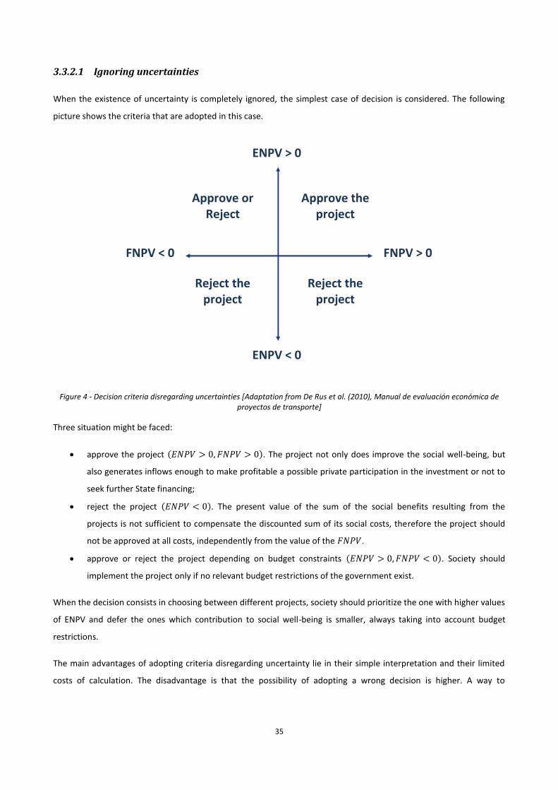
35
3.3.2.1 Ignoring uncertainties
When the existence of uncertainty is completely ignored, the simplest case of decision is considered. The following
picture shows the criteria that are adopted in this case.
Figure 4 - Decision criteria disregarding uncertainties [Adaptation from De Rus et al. (2010), Manual de evaluación económica de proyectos de transporte]
Three situation might be faced:
approve the project (𝐸𝑁𝑃𝑉 > 0, 𝐹𝑁𝑃𝑉 > 0). The project not only does improve the social well-being, but
also generates inflows enough to make profitable a possible private participation in the investment or not to
seek further State financing;
reject the project (𝐸𝑁𝑃𝑉 < 0). The present value of the sum of the social benefits resulting from the
projects is not sufficient to compensate the discounted sum of its social costs, therefore the project should
not be approved at all costs, independently from the value of the 𝐹𝑁𝑃𝑉.
approve or reject the project depending on budget constraints (𝐸𝑁𝑃𝑉 > 0, 𝐹𝑁𝑃𝑉 < 0). Society should
implement the project only if no relevant budget restrictions of the government exist.
When the decision consists in choosing between different projects, society should prioritize the one with higher values
of ENPV and defer the ones which contribution to social well-being is smaller, always taking into account budget
restrictions.
The main advantages of adopting criteria disregarding uncertainty lie in their simple interpretation and their limited
costs of calculation. The disadvantage is that the possibility of adopting a wrong decision is higher. A way to
Approve the project
Reject the project
Reject the project
Approve or Reject
FNPV > 0
FNPV < 0
ENPV > 0
ENPV < 0
36
supplement this process, typically used in conventional CBA technics, is to add a sensitivity analysis, to see how and
how much the NPV varies modifying certain parameters.
3.3.2.2 Criteria under uncertainty
When uncertainty is considered in the evaluation, in addition to the expected value of the NPV, the decision-taker is
provided with the probability distribution of the NPV. This information is quite useful for the private sector, usually
adverse to risk.
For the public sector, no all the theories agree about whether it should be neutral to risk or not. The most general
position is the one based on the Arrow-Lind Theorem, according to which the sharing of the risk between a very high
number of people make its cost tend to zero. When these conditions consist, it makes sense to work with expected
values.
Coming back to decision taking considering uncertainty, basically, when the probability distribution of the ENPV does
not show any positive value, the project must be rejected. When, instead, all the values shown are positive, the
project should be approved. When the distribution covers both positive and negative values, the expected value
should be examined, approving those project having:
𝐸(𝐸𝑁𝑃𝑉) ≥ 0, ( 10 )
where 𝐸(𝐸𝑁𝑃𝑉) denotes the expected value of 𝐸𝑁𝑃𝑉.
This still simple criterion is adequate in the cases where no budget restrictions exist and the decision-taker is neutral
to risk.
When the risk associated to the probability of obtaining a negative 𝐸𝑁𝑃𝑉 is relevant for the decision-taker, all the
information deriving from the probability distribution should be included in the decision process and the decision to
approve or reject the project shall depend on the risk threshold that he is prone to accept. The threshold may be
measured in terms of the tolerance level to negative results (probability 𝛼). So, 𝐹𝐸𝑁𝑃𝑉 represents the cumulate
probability function of the 𝐸𝑁𝑃𝑉 (distribution function) and 𝐹𝐸𝑁𝑃𝑉(0) the probability that 𝐸𝑁𝑃𝑉 is negative.
Therefore, the project should be approved only if
𝐹𝐸𝑁𝑃𝑉(0) ≤ 𝛼, ( 11 )
as it is shown in the following picture, where it is considered that the critical value 𝛼 has to be fixed exogenously and
before carrying out the evaluation.
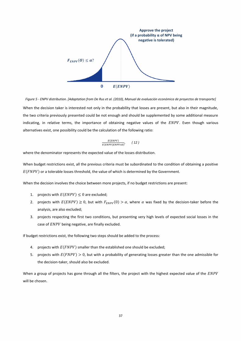
37
Figure 5 - ENPV distribution. [Adaptation from De Rus et al. (2010), Manual de evaluación económica de proyectos de transporte]
When the decision taker is interested not only in the probability that losses are present, but also in their magnitude,
the two criteria previously presented could be not enough and should be supplemented by some additional measure
indicating, in relative terms, the importance of obtaining negative values of the 𝐸𝑁𝑃𝑉. Even though various
alternatives exist, one possibility could be the calculation of the following ratio:
𝐸(𝐸𝑁𝑃𝑉)
𝐸(𝐸𝑁𝑃𝑉|𝐸𝑁𝑃𝑉≤0), ( 12 )
where the denominator represents the expected value of the losses distribution.
When budget restrictions exist, all the previous criteria must be subordinated to the condition of obtaining a positive
𝐸(𝐹𝑁𝑃𝑉) or a tolerable losses threshold, the value of which is determined by the Government.
When the decision involves the choice between more projects, if no budget restrictions are present:
1. projects with 𝐸(𝐸𝑁𝑃𝑉) ≤ 0 are excluded;
2. projects with 𝐸(𝐸𝑁𝑃𝑉) ≥ 0, but with 𝐹𝐸𝑁𝑃𝑉(0) > 𝛼, where 𝛼 was fixed by the decision-taker before the
analysis, are also excluded;
3. projects respecting the first two conditions, but presenting very high levels of expected social losses in the
case of 𝐸𝑁𝑃𝑉 being negative, are finally excluded.
If budget restrictions exist, the following two steps should be added to the process:
4. projects with 𝐸(𝐹𝑁𝑃𝑉) smaller than the established one should be excluded;
5. projects with 𝐸(𝐹𝑁𝑃𝑉) > 0, but with a probability of generating losses greater than the one admissible for
the decision-taker, should also be excluded.
When a group of projects has gone through all the filters, the project with the highest expected value of the 𝐸𝑁𝑃𝑉
will be chosen.
Approve the project (if a probability α of NPV being
negative is tolerated)
𝑭𝑬𝑵𝑷𝑽(𝑶) ≤ 𝜶?
𝑬(𝑬𝑵𝑷𝑽)
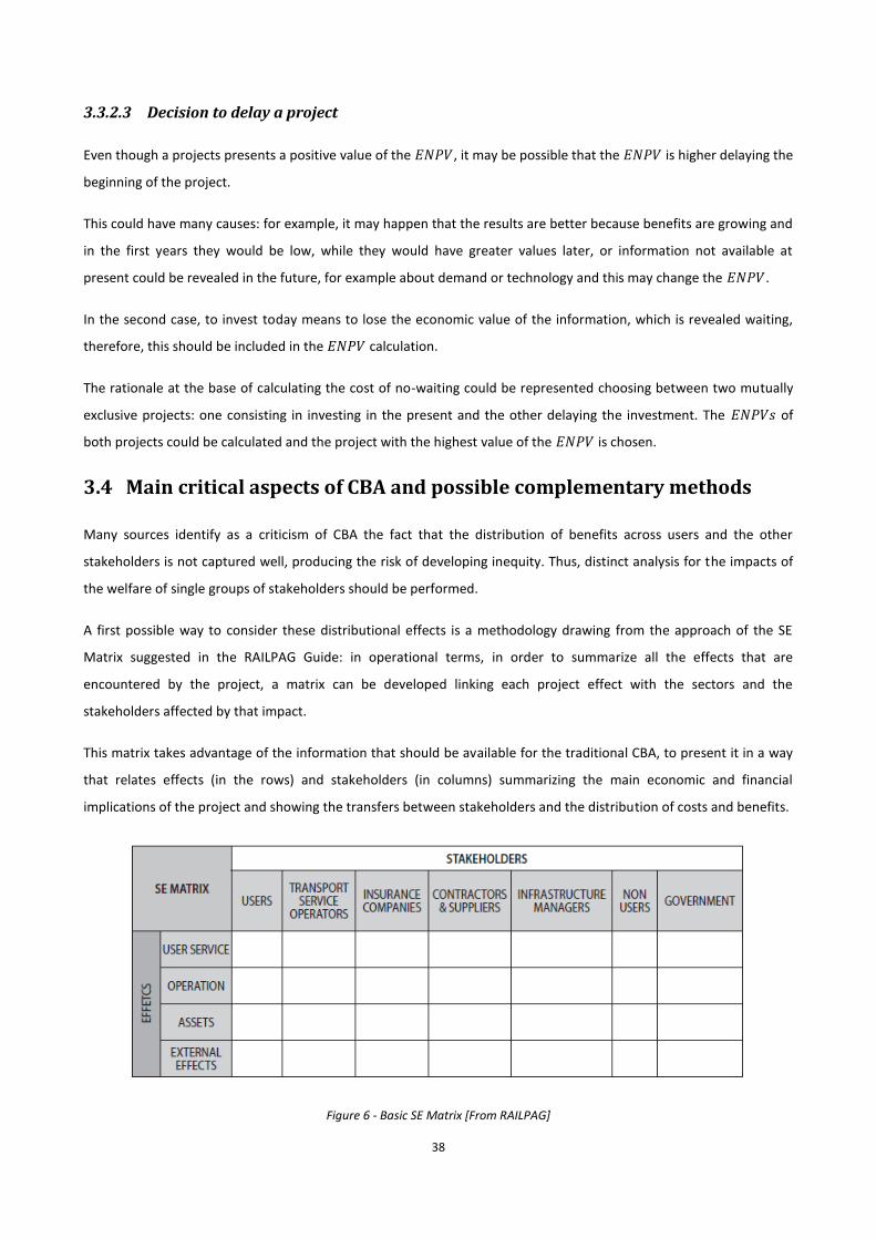
38
3.3.2.3 Decision to delay a project
Even though a projects presents a positive value of the 𝐸𝑁𝑃𝑉, it may be possible that the 𝐸𝑁𝑃𝑉 is higher delaying the
beginning of the project.
This could have many causes: for example, it may happen that the results are better because benefits are growing and
in the first years they would be low, while they would have greater values later, or information not available at
present could be revealed in the future, for example about demand or technology and this may change the 𝐸𝑁𝑃𝑉.
In the second case, to invest today means to lose the economic value of the information, which is revealed waiting,
therefore, this should be included in the 𝐸𝑁𝑃𝑉 calculation.
The rationale at the base of calculating the cost of no-waiting could be represented choosing between two mutually
exclusive projects: one consisting in investing in the present and the other delaying the investment. The 𝐸𝑁𝑃𝑉𝑠 of
both projects could be calculated and the project with the highest value of the 𝐸𝑁𝑃𝑉 is chosen.
3.4 Main critical aspects of CBA and possible complementary methods
Many sources identify as a criticism of CBA the fact that the distribution of benefits across users and the other
stakeholders is not captured well, producing the risk of developing inequity. Thus, distinct analysis for the impacts of
the welfare of single groups of stakeholders should be performed.
A first possible way to consider these distributional effects is a methodology drawing from the approach of the SE
Matrix suggested in the RAILPAG Guide: in operational terms, in order to summarize all the effects that are
encountered by the project, a matrix can be developed linking each project effect with the sectors and the
stakeholders affected by that impact.
This matrix takes advantage of the information that should be available for the traditional CBA, to present it in a way
that relates effects (in the rows) and stakeholders (in columns) summarizing the main economic and financial
implications of the project and showing the transfers between stakeholders and the distribution of costs and benefits.
Figure 6 - Basic SE Matrix [From RAILPAG]
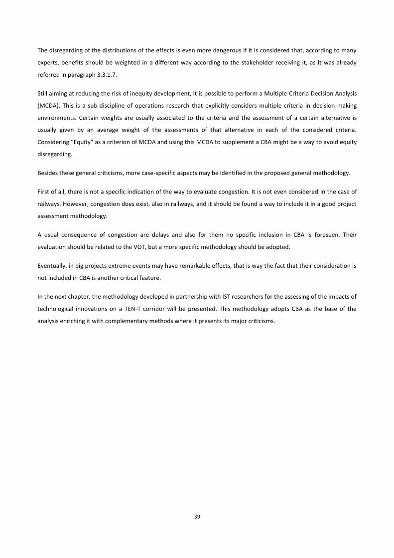
39
The disregarding of the distributions of the effects is even more dangerous if it is considered that, according to many
experts, benefits should be weighted in a different way according to the stakeholder receiving it, as it was already
referred in paragraph 3.3.1.7.
Still aiming at reducing the risk of inequity development, it is possible to perform a Multiple-Criteria Decision Analysis
(MCDA). This is a sub-discipline of operations research that explicitly considers multiple criteria in decision-making
environments. Certain weights are usually associated to the criteria and the assessment of a certain alternative is
usually given by an average weight of the assessments of that alternative in each of the considered criteria.
Considering “Equity” as a criterion of MCDA and using this MCDA to supplement a CBA might be a way to avoid equity
disregarding.
Besides these general criticisms, more case-specific aspects may be identified in the proposed general methodology.
First of all, there is not a specific indication of the way to evaluate congestion. It is not even considered in the case of
railways. However, congestion does exist, also in railways, and it should be found a way to include it in a good project
assessment methodology.
A usual consequence of congestion are delays and also for them no specific inclusion in CBA is foreseen. Their
evaluation should be related to the VOT, but a more specific methodology should be adopted.
Eventually, in big projects extreme events may have remarkable effects, that is way the fact that their consideration is
not included in CBA is another critical feature.
In the next chapter, the methodology developed in partnership with IST researchers for the assessing of the impacts of
technological innovations on a TEN-T corridor will be presented. This methodology adopts CBA as the base of the
analysis enriching it with complementary methods where it presents its major criticisms.
40
4. APPROACH TO ASSESS THE IMPACT OF
TECHNOLOGICAL INNOVATIONS
The challenge of this chapter is trying to develop an assessment methodology to evaluate the profitability of a certain
combination of investments along a TEN-T corridor, assessing the impacts of technological innovations to be
developed under C4R project.
The assessment tool is made up by a spreadsheet. One of its main features is the fact that it must be easily adaptable
to the different corridors.
4.1 Main features of the approach
In view of the above, it is clear that we are not dealing with an ordinary investment appraisal:
first of all, the geographic scope of every analysis is extremely wide. Every corridor crosses more than one
country, each of them having different social, economic, political and institutional contexts. Also the technical
and operational characteristics of the railways may present big differences between the countries;
the analyzed investments are made up by dozens of individual projects, characterized by different locations,
timing, budgets and stakeholders;
the considered investments are based on the implementation of technologies that are still under
development, meaning that much about them is just estimated, including their costs of implementation and
maintenance, their installation rates and the year of achieving of Technology Readiness Level (TRL) 9, which is
the level corresponding to “system ready for full scale deployment”, being the maximum TRL in a scale of 9;
Figure 7 - Technology Readiness Level (TRL) scale.
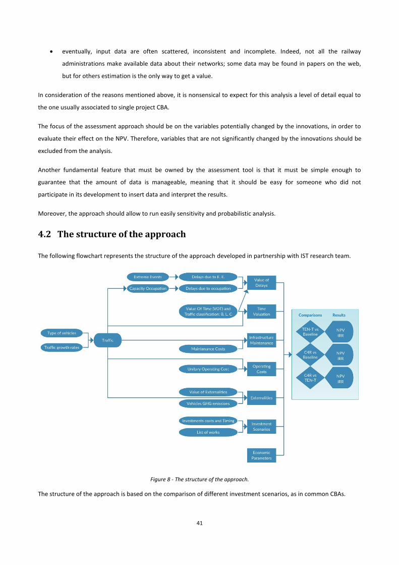
41
eventually, input data are often scattered, inconsistent and incomplete. Indeed, not all the railway
administrations make available data about their networks; some data may be found in papers on the web,
but for others estimation is the only way to get a value.
In consideration of the reasons mentioned above, it is nonsensical to expect for this analysis a level of detail equal to
the one usually associated to single project CBA.
The focus of the assessment approach should be on the variables potentially changed by the innovations, in order to
evaluate their effect on the NPV. Therefore, variables that are not significantly changed by the innovations should be
excluded from the analysis.
Another fundamental feature that must be owned by the assessment tool is that it must be simple enough to
guarantee that the amount of data is manageable, meaning that it should be easy for someone who did not
participate in its development to insert data and interpret the results.
Moreover, the approach should allow to run easily sensitivity and probabilistic analysis.
4.2 The structure of the approach
The following flowchart represents the structure of the approach developed in partnership with IST research team.
Figure 8 - The structure of the approach.
The structure of the approach is based on the comparison of different investment scenarios, as in common CBAs.
42
One of the scenarios will always be given by the “Do-minimum scenario”, in this approach called “Baseline”. This
scenario does not foresee any investment but the ones due to the end of the useful life of parts of the infrastructure
and assets.
The TEN-T scenario is also always considered and it includes the investments listed in the TEN-T corridor reports,
available on the European Commission website.
Then, C4R investments are considered. When C4R innovations are foreseen, it is always considered that also TEN-T
investments are executed, meaning the adoption of an incremental approach. However, many combinations of
different C4R technologies in different locations are considered, creating thus many C4R scenarios. This is done mainly
to find out which combination would be the most profitable.
The comparison is based on the elements represented with rectangles: costs and benefits deriving from Investments
scenarios, Externalities, Operating costs, Infrastructure maintenance, Time valuation and Value of Delays are summed
up and discounted according to the economic parameters.
In the following paragraphs, each part of the structure will be analyzed and described.
4.3 Input Data
The inputs of the analysis play a fundamental role, because they may have a rather big effect on the final value of the
NPV. That is why an entire part of the C4R project is dedicated just to the elaboration of the inputs to be used for the
assessment. However, nowadays many of these studies about the inputs are not available yet and for the present
work many of them were just estimated.
Most of the costs estimations were based on the available literature, especially Baumgartner J.P., 2001. Prices and
Costs in the railway sector; Flodén J., 2011, Rail Freight Costs and Michas G., 2012. Slab Track Systems for High-Speed
Railways with the collaboration of IST research team.
The following paragraphs will report the main strategies adopted in order to get significant data to be used in the
analysis.
4.3.1 Sections, traffic and list of works
European Commission takes care of elaborating periodical reports about its core network rail corridors. These reports
constitute a very precious source of information to be used as inputs for the scope of the analysis.
First of all, the reports include a very clear description of the structure of the network, which allows to elaborate the
list of the sections in which the network is divided, each of them with the indication of the nods of start and end of the
section and its total length. The network segmentation is applied both to the railways network and the roads one,
nevertheless the two segmentations may differ somehow. This constitutes a first complication, that can be easily
solved considering the real geography of the region.
43
The reports contain also traffic projections. Actually, they have to be considered as demand projections, foreseeing
the future evolution of demand, in absence of any important investment. Sometimes they are based on public reports,
while sometimes they are directly offered by the infrastructures managers. Since these traffic data come from
different sources, they are often expressed in different units, for example trains per day in some cases and passengers
per day in others. This fact leads to complications because some of the data have to be adapted to the other unit in
order to work with them.
The character of these traffic projections is always very simplistic, because just the values of traffic in two different
years are shown and the average annual growth rate is estimated considering a linear growth. The fact that the two
years for which traffic is shown do not coincide in the projections for all the lines constitutes another complication.
Another very important piece of information available in the report is given by the list of projects. It contains the
transport mode considered, a brief description of the project, the timing, the costs and other information. The list of
projects is useful for the construction of the TEN-T scenario, because it includes all the projects considered for TEN-T
innovations.
4.3.2 Value of time and of externalities
For value of time and externalities, it was chosen to rely on the values referred in HEATCO, a document published in
2006 whose objective was to propose harmonized guidelines for project assessment for trans-national projects in
Europe.
As it was referred in chapter 3, the main CBA guidelines, including the ones by EC, suggest to rely on this document
when no more recent studies developed in the specific country under analysis are available.
Both values for VOT and GHG emissions are included in this document. VOT values depend on the country considered,
while GHG emission monetary value is independent on the country due to the global character of this externality.
All the values in this manual are expressed in € of 2001 and, in order to be used for the analysis, they should be
actualized. A possible way to do so is through the consideration of the variation of the Consumer Price Index (CPI).
4.3.3 Economic parameters
Regarding these parameters, they show a character which is slightly different from the ones previously referred.
Indeed, they do not belong to the technical field, but rather to the economy word. However, their influence on the
final result of the analysis may be great.
The first of them is the time horizon of the analysis amounting to 40 years. This value is rather typical for railway
investment projects.
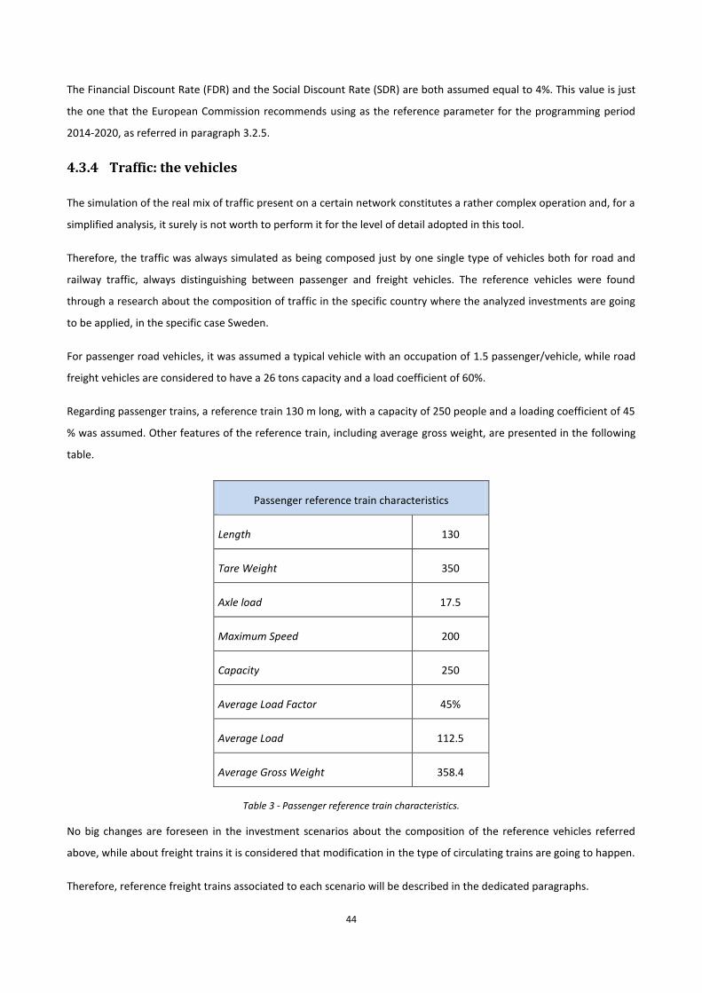
44
The Financial Discount Rate (FDR) and the Social Discount Rate (SDR) are both assumed equal to 4%. This value is just
the one that the European Commission recommends using as the reference parameter for the programming period
2014-2020, as referred in paragraph 3.2.5.
4.3.4 Traffic: the vehicles
The simulation of the real mix of traffic present on a certain network constitutes a rather complex operation and, for a
simplified analysis, it surely is not worth to perform it for the level of detail adopted in this tool.
Therefore, the traffic was always simulated as being composed just by one single type of vehicles both for road and
railway traffic, always distinguishing between passenger and freight vehicles. The reference vehicles were found
through a research about the composition of traffic in the specific country where the analyzed investments are going
to be applied, in the specific case Sweden.
For passenger road vehicles, it was assumed a typical vehicle with an occupation of 1.5 passenger/vehicle, while road
freight vehicles are considered to have a 26 tons capacity and a load coefficient of 60%.
Regarding passenger trains, a reference train 130 m long, with a capacity of 250 people and a loading coefficient of 45
% was assumed. Other features of the reference train, including average gross weight, are presented in the following
table.
Passenger reference train characteristics
Length 130
Tare Weight 350
Axle load 17.5
Maximum Speed 200
Capacity 250
Average Load Factor 45%
Average Load 112.5
Average Gross Weight 358.4
Table 3 - Passenger reference train characteristics.
No big changes are foreseen in the investment scenarios about the composition of the reference vehicles referred
above, while about freight trains it is considered that modification in the type of circulating trains are going to happen.
Therefore, reference freight trains associated to each scenario will be described in the dedicated paragraphs.
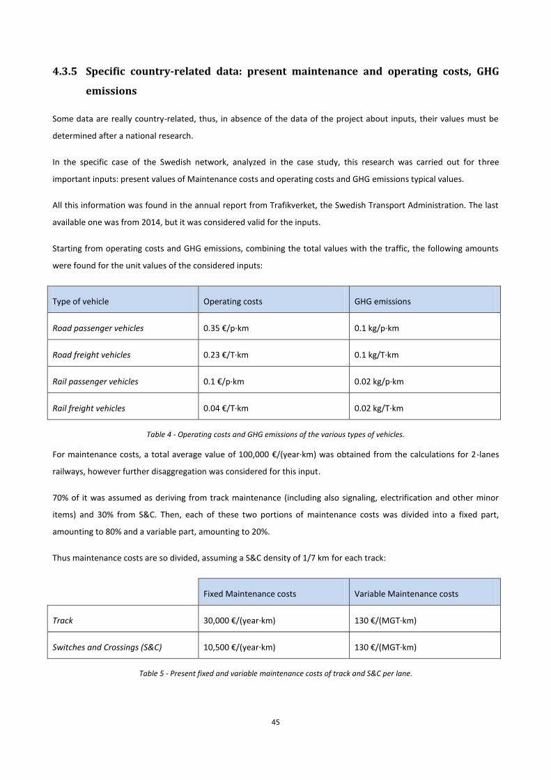
45
4.3.5 Specific country-related data: present maintenance and operating costs, GHG
emissions
Some data are really country-related, thus, in absence of the data of the project about inputs, their values must be
determined after a national research.
In the specific case of the Swedish network, analyzed in the case study, this research was carried out for three
important inputs: present values of Maintenance costs and operating costs and GHG emissions typical values.
All this information was found in the annual report from Trafikverket, the Swedish Transport Administration. The last
available one was from 2014, but it was considered valid for the inputs.
Starting from operating costs and GHG emissions, combining the total values with the traffic, the following amounts
were found for the unit values of the considered inputs:
Type of vehicle Operating costs GHG emissions
Road passenger vehicles 0.35 €/p·km 0.1 kg/p·km
Road freight vehicles 0.23 €/T·km 0.1 kg/T·km
Rail passenger vehicles 0.1 €/p·km 0.02 kg/p·km
Rail freight vehicles 0.04 €/T·km 0.02 kg/T·km
Table 4 - Operating costs and GHG emissions of the various types of vehicles.
For maintenance costs, a total average value of 100,000 €/(year·km) was obtained from the calculations for 2-lanes
railways, however further disaggregation was considered for this input.
70% of it was assumed as deriving from track maintenance (including also signaling, electrification and other minor
items) and 30% from S&C. Then, each of these two portions of maintenance costs was divided into a fixed part,
amounting to 80% and a variable part, amounting to 20%.
Thus maintenance costs are so divided, assuming a S&C density of 1/7 km for each track:
Fixed Maintenance costs Variable Maintenance costs
Track 30,000 €/(year·km) 130 €/(MGT·km)
Switches and Crossings (S&C) 10,500 €/(year·km) 130 €/(MGT·km)
Table 5 - Present fixed and variable maintenance costs of track and S&C per lane.
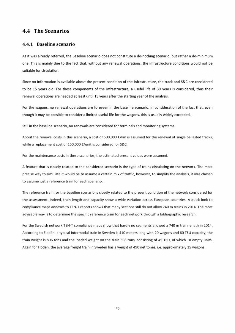
46
4.4 The Scenarios
4.4.1 Baseline scenario
As it was already referred, the Baseline scenario does not constitute a do-nothing scenario, but rather a do-minimum
one. This is mainly due to the fact that, without any renewal operations, the infrastructure conditions would not be
suitable for circulation.
Since no information is available about the present condition of the infrastructure, the track and S&C are considered
to be 15 years old. For these components of the infrastructure, a useful life of 30 years is considered, thus their
renewal operations are needed at least until 15 years after the starting year of the analysis.
For the wagons, no renewal operations are foreseen in the baseline scenario, in consideration of the fact that, even
though it may be possible to consider a limited useful life for the wagons, this is usually widely exceeded.
Still in the baseline scenario, no renewals are considered for terminals and monitoring systems.
About the renewal costs in this scenario, a cost of 500,000 €/km is assumed for the renewal of single ballasted tracks,
while a replacement cost of 150,000 €/unit is considered for S&C.
For the maintenance costs in these scenarios, the estimated present values were assumed.
A feature that is closely related to the considered scenario is the type of trains circulating on the network. The most
precise way to simulate it would be to assume a certain mix of traffic, however, to simplify the analysis, it was chosen
to assume just a reference train for each scenario.
The reference train for the baseline scenario is closely related to the present condition of the network considered for
the assessment. Indeed, train length and capacity show a wide variation across European countries. A quick look to
compliance maps annexes to TEN-T reports shows that many sections still do not allow 740 m trains in 2014. The most
advisable way is to determine the specific reference train for each network through a bibliographic research.
For the Swedish network TEN-T compliance maps show that hardly no segments allowed a 740 m train length in 2014.
According to Flodén, a typical intermodal train in Sweden is 410 meters long with 20 wagons and 60 TEU capacity; the
train weight is 806 tons and the loaded weight on the train 398 tons, consisting of 45 TEU, of which 18 empty units.
Again for Flodén, the average freight train in Sweden has a weight of 490 net tones, i.e. approximately 15 wagons.
47
Considering these data, the reference train of the baseline scenario could be described as so:
Baseline freight reference train characteristics
Length 400
Tare Weight 400
Axle Loas 22.5
Cargo Capacity 1,000
Average Load Factor 50%
Average Load 500
Average Gross Weight 900
Operating Cost 0.04
GHG Emissions 0.02
Table 6 - Baseline freight reference train characteristics.
4.4.2 TEN-T scenario
In this scenario, it is considered the realization of the works listed in the TEN-T report. Since in this list all the costs of
the projects are specified, no costs estimation is needed.
About the effects, the main ones regard the change of the typical freight train: a longer train is considered, meaning a
Higher Average Load and a higher Average Gross Weight, while smaller operational costs and GHG emissions are
considered.
Specifically, in the adopted case study, a 700 m train is considered, with an operating cost of 0.03 €/T·km and GHG
emissions of 0.018 kg/T·km, considering a 10% reduction compared with the Baseline Scenario.
4.4.3 C4R scenario: possible innovations costs and effects
The innovations that are going to be developed by C4R project and then possibly introduced in the existing network
are listed in the Description of Work of C4R. The main ones are:
the upgrade to slab track;
the replacement of switching and crossing;
the introduction of a new fleet of wagons with 25 t/axle, modern coupling, braking and intelligence;
the upgrade of interchanges;
48
the introduction of new monitoring systems.
All the new technologies are considered to reach TRL 9 in 2025 and to be applied in the same year.
Each of the listed innovations has specific costs and effects on the benefits. Unlike TEN-T projects, investments costs
are often unknown for C4R innovations and estimations are necessary.
4.4.3.1 Slab track
No C4R files are yet available regarding slab track implementation costs. However, most slab track designs nowadays
cost 750 to 1,100 €/meter. Thus, a medium value of 1,000 €/meter was assumed in the deterministic analysis, giving
rise to a cost of 1,000,000 €/km.
The main effects associated to an upgrade to slab track are connected to the need of less maintenance and, thus, the
reduction of the variable maintenance costs. Specifically, the introduction of slab track is considered to decrease the
present variable maintenance costs to just the half of it. The values considered are so 130 €/(MGT km) for Baseline
and TEN-T scenarios and 65 €/(MGT km) for the scenarios involving the introduction of this first innovation.
4.4.3.2 Upgrade of interchanges
About the upgrade of the interchanges, a final document is already available. An average investment cost of 100
M€/terminal may be assumed.
The real consequences of the upgrade of a terminal seem quite difficult to determine in detail, therefore a simplified
approach has to be assumed.
Surely, the benefit deriving from this innovation has to be sought in the operating costs: one of the main effects of the
upgrade for the terminal would be quicker loading and unloading operations, meaning the employment of less people
in the terminals to execute the same work. Since no detailed information is available about this, a reduction of the
operating costs of freight railway transport in the order of 10% is assumed as a consequence of this innovation.
Quicker loading and unloading operation can be considered also through a reduction of freight trains travel time,
assumed in the order of 5%.
4.4.3.3 Switches and crossings (S&C)
Also about S&C, no C4R files are available yet, thus both costs and effects have to be estimated. As it was referred in
paragraph 4.4.1, the cost of the replacement of S&C is nowadays around 150,000 €, showing a great variability
according to their geometric characteristics (as radius, tangent and length), which are closely related to the allowed
speed.
As a very rough approximation, an installation cost equal to the double of the present average value can be assumed,
thus 300,000 €/unit will be the considered value.
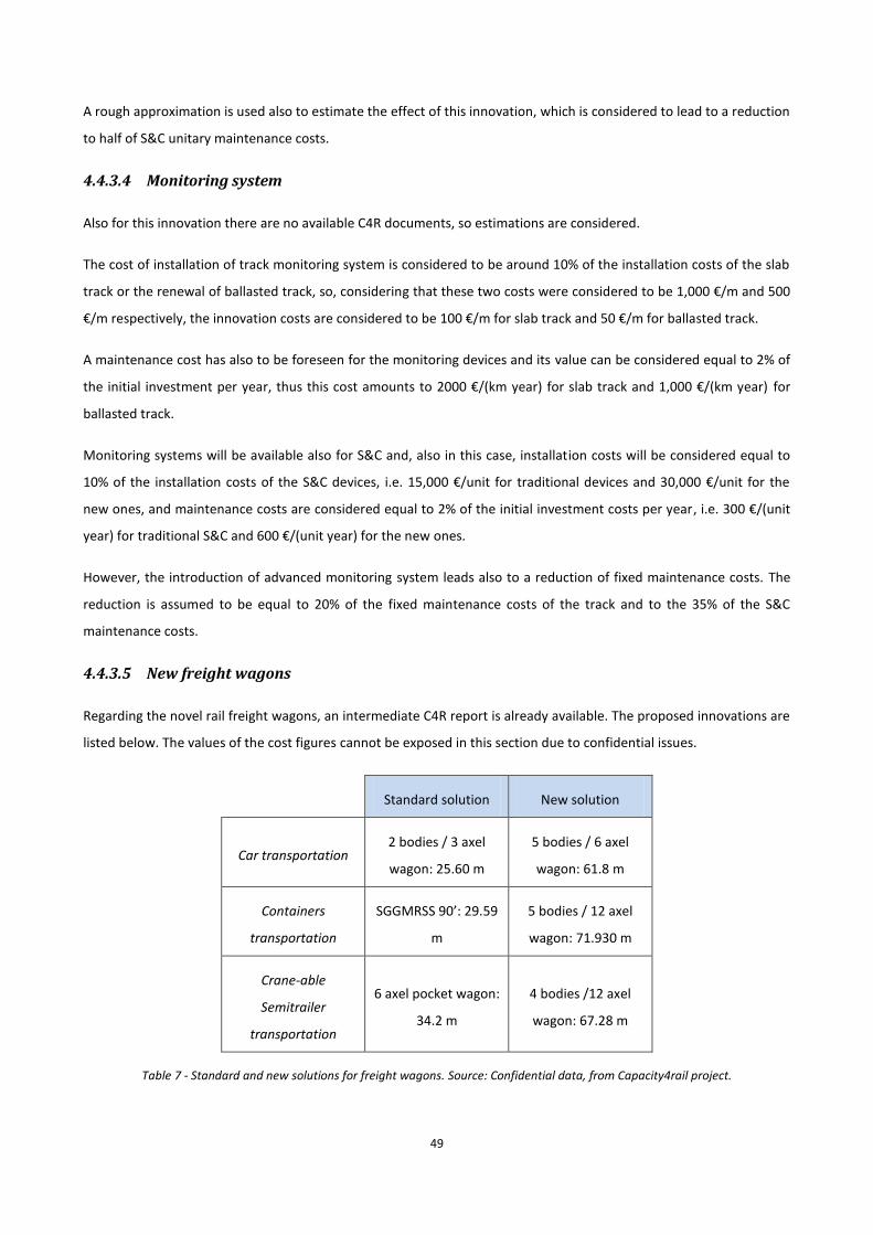
49
A rough approximation is used also to estimate the effect of this innovation, which is considered to lead to a reduction
to half of S&C unitary maintenance costs.
4.4.3.4 Monitoring system
Also for this innovation there are no available C4R documents, so estimations are considered.
The cost of installation of track monitoring system is considered to be around 10% of the installation costs of the slab
track or the renewal of ballasted track, so, considering that these two costs were considered to be 1,000 €/m and 500
€/m respectively, the innovation costs are considered to be 100 €/m for slab track and 50 €/m for ballasted track.
A maintenance cost has also to be foreseen for the monitoring devices and its value can be considered equal to 2% of
the initial investment per year, thus this cost amounts to 2000 €/(km year) for slab track and 1,000 €/(km year) for
ballasted track.
Monitoring systems will be available also for S&C and, also in this case, installation costs will be considered equal to
10% of the installation costs of the S&C devices, i.e. 15,000 €/unit for traditional devices and 30,000 €/unit for the
new ones, and maintenance costs are considered equal to 2% of the initial investment costs per year, i.e. 300 €/(unit
year) for traditional S&C and 600 €/(unit year) for the new ones.
However, the introduction of advanced monitoring system leads also to a reduction of fixed maintenance costs. The
reduction is assumed to be equal to 20% of the fixed maintenance costs of the track and to the 35% of the S&C
maintenance costs.
4.4.3.5 New freight wagons
Regarding the novel rail freight wagons, an intermediate C4R report is already available. The proposed innovations are
listed below. The values of the cost figures cannot be exposed in this section due to confidential issues.
Standard solution New solution
Car transportation 2 bodies / 3 axel
wagon: 25.60 m
5 bodies / 6 axel
wagon: 61.8 m
Containers
transportation
SGGMRSS 90’: 29.59
m
5 bodies / 12 axel
wagon: 71.930 m
Crane-able
Semitrailer
transportation
6 axel pocket wagon:
34.2 m
4 bodies /12 axel
wagon: 67.28 m
Table 7 - Standard and new solutions for freight wagons. Source: Confidential data, from Capacity4rail project.

50
The total investment cost should be calculated considering the replacement of the whole existing present fleet, basing
on the present transport tonnage capacity.
Since no information is available about the capacity of the new wagons, but just regarding their length, it will be
assumed that the capacity of the new wagons is the double of the old ones’, meaning that just half of the present
number of wagons will be needed.
The main effects of the introduction of the new wagons are, first of all, the reduction of the number of wagons
needed, due to their larger capacity (bigger wagons and higher axel load), and the reduction of the operational costs,
in the order of 10% compared to the TEN–T value.
Unlike the innovations previously presented, when a small network is considered, the replacement of the wagons is
considered to be applied to the entire network.
If, in some scenarios, wagons replacement is not combined with the upgrade to slab track in any part of the network,
maintenance costs should be considered to increase in those parts as an effect of the circulation of wagons with a
higher axle load. In these cases, a renewal of the track is programmed before the introduction of the new wagons and,
then, the maintenance costs are considered to be equal to the baseline values multiplied by the factor (25/22.5)2, i.e.
the square of the ratio between the new axle load and the born one.
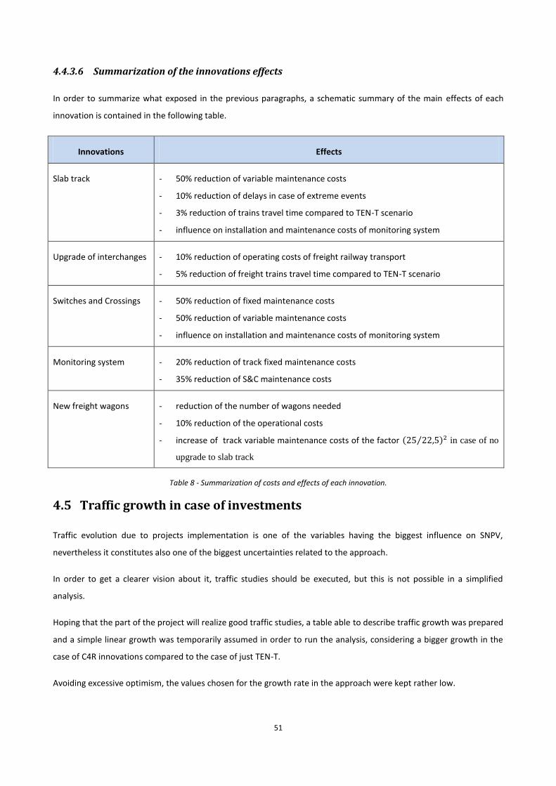
51
4.4.3.6 Summarization of the innovations effects
In order to summarize what exposed in the previous paragraphs, a schematic summary of the main effects of each
innovation is contained in the following table.
Innovations Effects
Slab track - 50% reduction of variable maintenance costs
- 10% reduction of delays in case of extreme events
- 3% reduction of trains travel time compared to TEN-T scenario
- influence on installation and maintenance costs of monitoring system
Upgrade of interchanges - 10% reduction of operating costs of freight railway transport
- 5% reduction of freight trains travel time compared to TEN-T scenario
Switches and Crossings - 50% reduction of fixed maintenance costs
- 50% reduction of variable maintenance costs
- influence on installation and maintenance costs of monitoring system
Monitoring system - 20% reduction of track fixed maintenance costs
- 35% reduction of S&C maintenance costs
New freight wagons - reduction of the number of wagons needed
- 10% reduction of the operational costs
- increase of track variable maintenance costs of the factor (25 22,5⁄ )2 in case of no
upgrade to slab track
Table 8 - Summarization of costs and effects of each innovation.
4.5 Traffic growth in case of investments
Traffic evolution due to projects implementation is one of the variables having the biggest influence on SNPV,
nevertheless it constitutes also one of the biggest uncertainties related to the approach.
In order to get a clearer vision about it, traffic studies should be executed, but this is not possible in a simplified
analysis.
Hoping that the part of the project will realize good traffic studies, a table able to describe traffic growth was prepared
and a simple linear growth was temporarily assumed in order to run the analysis, considering a bigger growth in the
case of C4R innovations compared to the case of just TEN-T.
Avoiding excessive optimism, the values chosen for the growth rate in the approach were kept rather low.
52
For TEN-T, it was assumed an annual traffic growth rate of 0.6% in diverted traffic from road to rail, while an annual
traffic growth rate of 0.2% was adopted for generated traffic.
For C4R, it was assumed an annual traffic growth rate of 1.2% in diverted traffic from road to rail, while an annual
traffic growth rate of 0.4% was adopted for generated traffic. As it was previously referred, C4R growth in both the
types of traffic is calculated in addition to the growth foreseen with just TEN-T.
4.6 Traffic: business, leisure, commuter
As it is widely known, the value of time (VOT) depends largely upon the purpose of the journey and passenger traffic
may be divided into three main categories: business, leisure and commuter trips.
The percentages corresponding to each category should be investigated by traffic studies, nevertheless in the present
work precise data about this classification are not available yet, thus typical percentages are assumed: it is considered
that 50% of passenger trips are for business purposes, 40% are commuter and 10% for leisure purposes.
4.7 Capacity occupation
A major parameter for the determination of the total amount of delays and the consequent losses of benefits is the
total capacity consumption.
It was decided to evaluate capacity consumption according to the guidelines contained in UIC 406 file.
These guidelines base the evaluation on the fraction of time during which the infrastructure results occupied.
The formula, as presented in UIC 406, is the following:
𝑘 = 𝐴 + 𝐵 + 𝐶 + 𝐷, ( 13 )
where:
𝑘 is the total consumption time [min];
𝐴 is the infrastructure occupation [min];
𝐵 is the buffer time [min];
𝐶 is the supplement for single-track lines [min];
𝐷 indicates the supplements for maintenance [min].
In percentage terms, we have:
𝐾 = 𝑘 ∙ 100/𝑈, ( 14 )
where:
𝐾 is the capacity consumption [%];
𝑈 is the chosen time window [min].
53
Once again, due to the scarcity of available data, the approach for this evaluation will be simplified.
In order to determine the infrastructure occupation, the block length is considered: for both passenger and freight
services, the number of trains per day is multiplied by the block length and then divided by the average speed and the
results are summed up. The obtained value is then multiplied for a factor including the buffer time and the crossing
buffer. The result is then divided by the number of tracks. The total supplement time for maintenance is then added
to the obtained value and the final result in percentage terms is got dividing by 24 and multiplying by 100. The
referred calculation can be expressed through the following formula:
𝐾 = {[(𝑃∙𝐵
𝑆𝑝+
𝐹∙𝐵
𝑆𝑓) ∙ (1 + 𝑏𝑡 + 𝑐𝑏) ∙
1
𝑛] + 𝑀} ∙
1
24∙ 100, ( 15 )
where:
𝐾 is the capacity consumption [%];
𝑃 is the number of passenger trains per day;
𝐹 is the number of freight trains per day;
𝐵 is the average block length in a specific section, assumed equal to 15 km, because a density of 1 S&C/7 km
is assumed;
𝑆𝑝 is the average speed of passenger trains in a certain section [km/h];
𝑆𝑓 is the average speed of freight trains in a certain section [km/h];
𝑏𝑡 is the increase due to the buffer time, assumed equal to 5%;
𝑐𝑏 is the increase due to the crossing buffer, assumed equal to 5% when the section is single-track;
𝑛 is the number of tracks;
𝑀 is the supplement time for maintenance, assumed equal to 5 hours.
Applying this formula to each section of the considered network, it is possible to determine a percentage
corresponding to the capacity consumption.
4.8 Reactionary delays
Obviously, high capacity consumption means a higher probability to show delays, called in this case reactionary
delays.
Among the models relating capacity occupation rate and delays, it was chosen to adopt a model presented by Stephen
Gibson, Grahame Cooper, and Brian Ball in the paper “Developments in transport policy: The evolution of capacity
charges on the UK rail network” (2002).
According to this study, the form that best fitted the observed data was an exponential one and the form of the
relationship chosen was:
𝐷𝑖𝑡 = 𝐴𝑖 ∙ 𝑒𝑥𝑝(𝛽 ∙ 𝐶𝑖𝑡), ( 16 )
54
where:
𝐷𝑖𝑡 is the reactionary delay on track section 𝑖 during time period 𝑡;
𝐴𝑖 is a route section specific constant;
𝛽 is a route specific constant;
𝐶𝑖𝑡 is the capacity occupation index (as defined above in paragraph 4.7) on track section 𝑖 during time period 𝑡.
One again, due to the scarcity of data for the network under analysis, the values of the constant in the formula will be
assumed, considering that the results of future studies will allow better estimations.
For the moment, a value of 1 is assumed for 𝐴𝑖, while a value of 2.5 is assumed for 𝛽, foreseeing to adjust the
parameters when reports from C4R will be available.
4.9 Extreme events
In order to the make the analysis more complete, it was chosen to include the modeling of extreme events. Typical
cases of extreme events that may happen in Sweden include flooding due to heavy rain or snow and ice. These
meteorological circumstances can add further delays to the ones predicted by capacity consumption.
A simple but clear model regarding the effects of precipitations on flooding of the railways was found in the master
thesis of Tim Gilbert, University of Birmingham.
This model relates the annual delay minutes (𝐷) with the monthly precipitation (𝑟𝑚 , 𝑖𝑛 𝑚𝑚) through the following
formula:
𝐷 = 370,4 ∙ ∑ (𝑟𝑚 − 80).12𝑚=1 ( 17 )
4.10 Monetary evaluation of delays
Delays result in an increase of time losses and, thus, in increasing costs. However, it is not correct to evaluate these
losses with the same VOT considered for travel time. In order to calculate the Total Costs of Travel Time Variability, it
is possible to use a formula proposed by one of the most advanced guidelines set for Transport Studies, the Transport
Analysis Guidance (DfT, 2011) provided by the UK Department of Transport (WebTAG).
The recommended formula is the following:
𝑇𝐶𝑇𝑇𝑉 = ∑ (𝛼 ∙ 𝐿+ + 𝛼 ∙ 𝛽 ∙ 𝑆𝐷+ + 𝛼 ∙ 𝑆𝐼 ∙ 1,5)𝑛 ∙ 𝑉𝑂𝑇𝑛 ∙ 𝑃𝑎𝑠𝑠𝑛 ( 18)
where:
𝑇𝐶𝑇𝑇𝑉 is the total cost of travel time variability;
𝛼 is the lateness factor (3 for umpredictable delays, 1 for predictable);
𝛽 is the reliability ratio (1.4 for trains and other PT, 0.8 for cars);
𝐿+ is the mean lateness;

55
𝑆𝐷+ is the standard deviation of travel times (the early arrivals are accounted as on time arrivals);
𝑆𝐼 is the service interval between the cancelled and the next train;
𝑉𝑂𝑇𝑛 is the Value Of Time (differentiated by the type of trip and user segment, if available);
𝑃𝑎𝑠𝑠𝑛 is the number of passangers (differentiated by the type of trip and user segment, if available).
UK Passenger Demand Forecasting Handbook states that only 25% of passengers are aware of advertised delay, thus 𝛼
should be calculated like this:
𝛼 = 0,25 ∙ 1 + 0,75 ∙ 3 = 2,5, ( 19 )
while 𝑆𝐼 could be determined from the mean interval between train passages.
4.11 The comparisons: C4R vs Baseline, C4R vs TEN-T
Finally, it is worth to describe the way profitability is evaluated.
In order to evaluate the profitability of each scenario involving C4R investments, the total net benefits produced by
the implementation of C4R innovations were compared both to the ones produced in the Baseline scenario and to the
ones produced in the TEN-T scenario.
Of course, the first difference is always bigger than the second one, because in the second case much more benefits
are produced.
Also the profitability of TEN-T was taken into account, comparing the total net benefits of this scenario to the ones of
Baseline.
All the results related to various scenarios and the respective considerations are collected in the following chapter.
56
5. APPLICATION TO SWEDISH CASE STUDY
With this chapter, the reader is entering maybe the most interesting part of the work, that is the one where the tool
elaborated basing on the theoretical assumptions presented above is used to evaluate the profitability of different
investments scenarios.
As it was already referred, for the application of the tool, a restricted geographic area was chosen, thus the analysis
was applied just to the Swedish part of the Scandinavian – Mediterranean Core Network corridor. This choice is mainly
justified by the fact that this part of the corridor, being slightly isolated, appeared to be the part where it was less
complex to test the tool.
First of all, some brief considerations about the building of the scenarios must be presented.
5.1 Preliminary considerations about the building of scenarios
As it was already referred, the main innovations introduced by C4R, i.e. the ones considered for the building of the
scenarios, are:
the upgrade to slab track;
the replacement of switches and crossings;
the introduction of a new fleet of wagons with 25 t/axle, modern coupling, braking and intelligence;
the upgrade of interchanges;
the introduction of new monitoring systems.
Each of the mentioned innovations has its own costs and benefits, that are presented in paragraph 4.4.3.
Theoretically, considering that it is possible to apply or not each one of the innovations to each segment of the
considered network and that every combination thus obtained might be considered as a different scenario, the
number of possible scenarios possibly obtained would be rather high. However, some considerations can lead us to
cut the number of scenarios, excluding the ones that do not make sense.
First of all, it must be considered, as it was outlined, that, theoretically, innovations may be applied globally, that is
involving the whole network, or locally, that is just in some segments. Nevertheless, some innovations do not make
much sense if applied just locally in this study. For example, it is the case of freight wagons replacement, due to the
small dimensions of the considered network. Also the upgrade of isolated interchanges will not be considered as a real
possibility.
Regarding the other innovations, it can make sense to apply them just in some sections, but, in case it is decided to
invest on local upgrades, the choice of the sections should be based on some rationale. In this study, it was chosen to
investigate the effects of local innovations on the segments characterized by the biggest traffic rates, based on the
traffic occupation table.
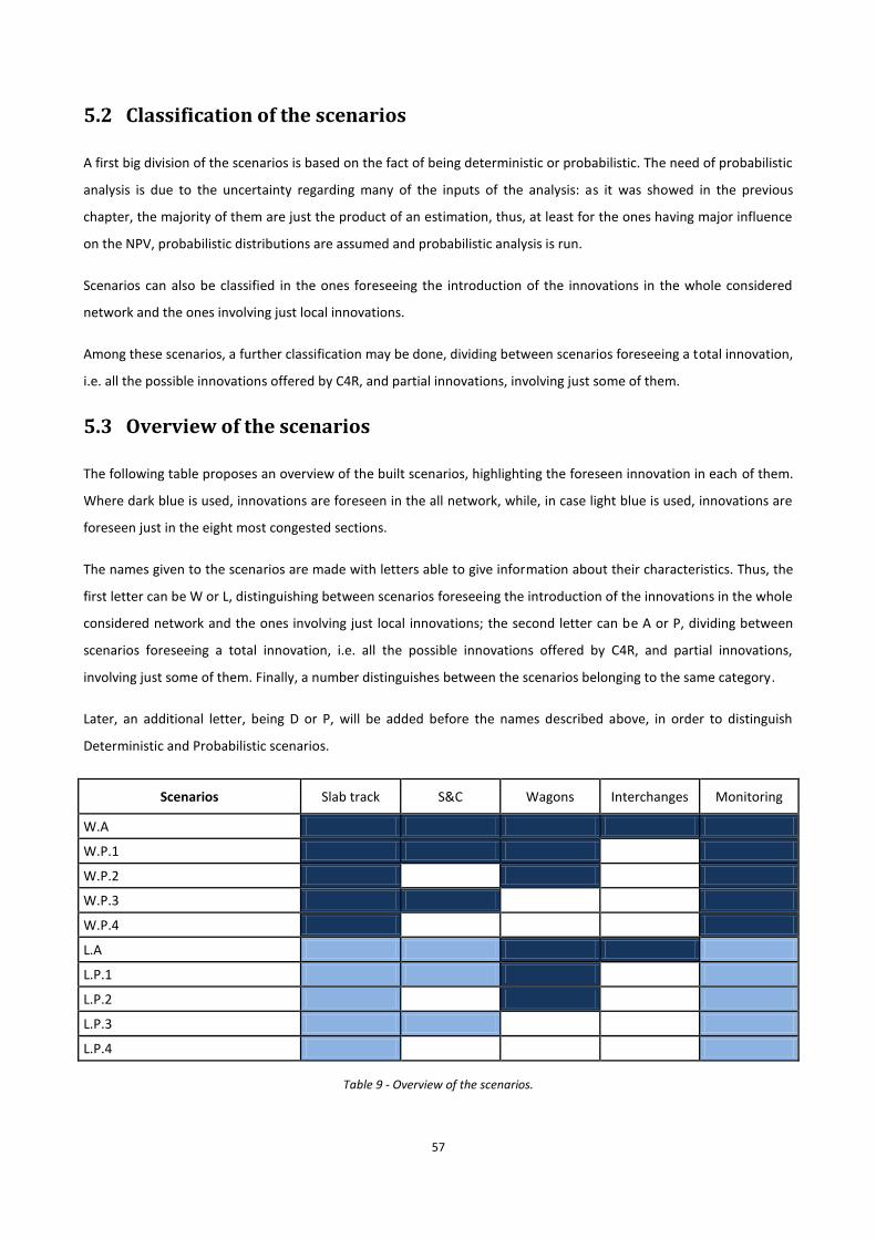
57
5.2 Classification of the scenarios
A first big division of the scenarios is based on the fact of being deterministic or probabilistic. The need of probabilistic
analysis is due to the uncertainty regarding many of the inputs of the analysis: as it was showed in the previous
chapter, the majority of them are just the product of an estimation, thus, at least for the ones having major influence
on the NPV, probabilistic distributions are assumed and probabilistic analysis is run.
Scenarios can also be classified in the ones foreseeing the introduction of the innovations in the whole considered
network and the ones involving just local innovations.
Among these scenarios, a further classification may be done, dividing between scenarios foreseeing a total innovation,
i.e. all the possible innovations offered by C4R, and partial innovations, involving just some of them.
5.3 Overview of the scenarios
The following table proposes an overview of the built scenarios, highlighting the foreseen innovation in each of them.
Where dark blue is used, innovations are foreseen in the all network, while, in case light blue is used, innovations are
foreseen just in the eight most congested sections.
The names given to the scenarios are made with letters able to give information about their characteristics. Thus, the
first letter can be W or L, distinguishing between scenarios foreseeing the introduction of the innovations in the whole
considered network and the ones involving just local innovations; the second letter can be A or P, dividing between
scenarios foreseeing a total innovation, i.e. all the possible innovations offered by C4R, and partial innovations,
involving just some of them. Finally, a number distinguishes between the scenarios belonging to the same category.
Later, an additional letter, being D or P, will be added before the names described above, in order to distinguish
Deterministic and Probabilistic scenarios.
Scenarios Slab track S&C Wagons Interchanges Monitoring
W.A
W.P.1
W.P.2
W.P.3
W.P.4
L.A
L.P.1
L.P.2
L.P.3
L.P.4
Table 9 - Overview of the scenarios.
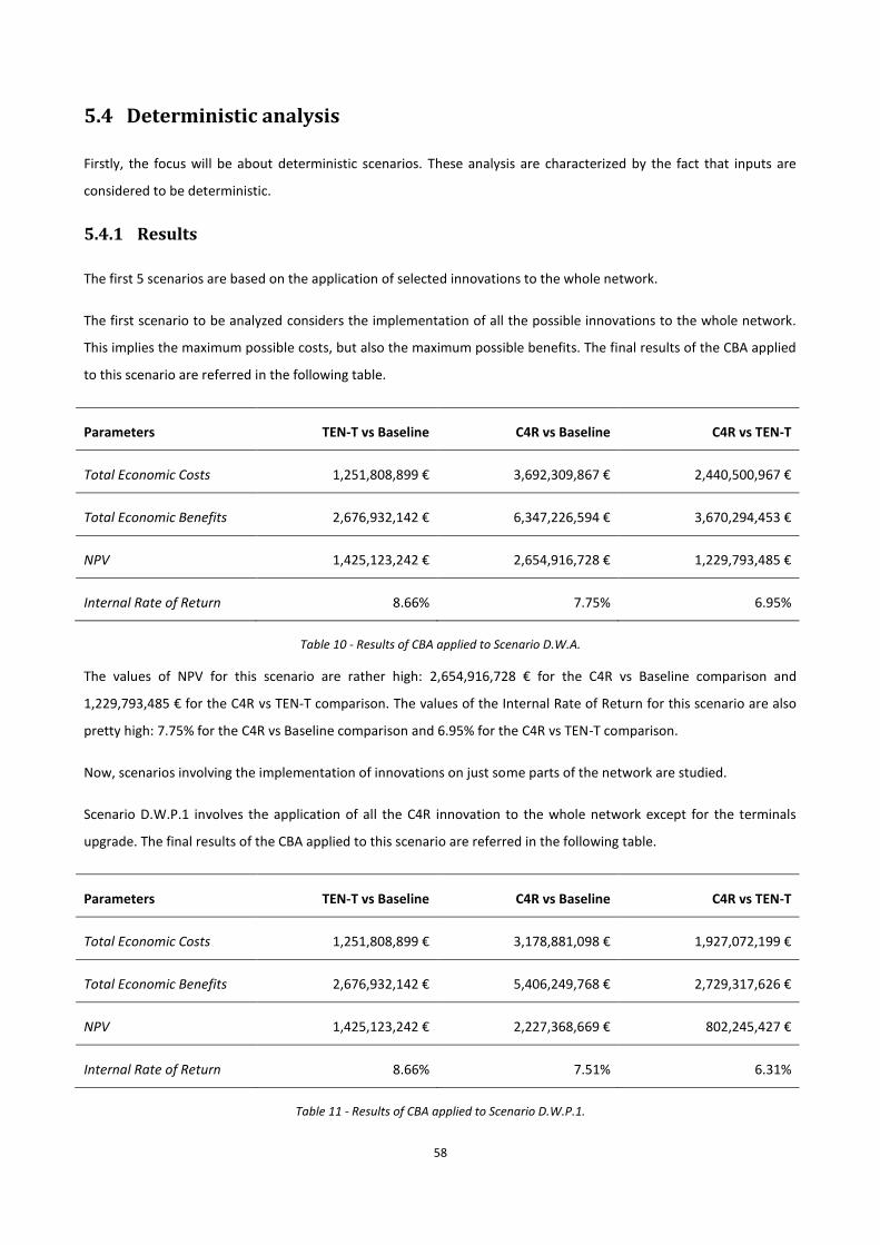
58
5.4 Deterministic analysis
Firstly, the focus will be about deterministic scenarios. These analysis are characterized by the fact that inputs are
considered to be deterministic.
5.4.1 Results
The first 5 scenarios are based on the application of selected innovations to the whole network.
The first scenario to be analyzed considers the implementation of all the possible innovations to the whole network.
This implies the maximum possible costs, but also the maximum possible benefits. The final results of the CBA applied
to this scenario are referred in the following table.
Parameters TEN-T vs Baseline C4R vs Baseline C4R vs TEN-T
Total Economic Costs 1,251,808,899 € 3,692,309,867 € 2,440,500,967 €
Total Economic Benefits 2,676,932,142 € 6,347,226,594 € 3,670,294,453 €
NPV 1,425,123,242 € 2,654,916,728 € 1,229,793,485 €
Internal Rate of Return 8.66% 7.75% 6.95%
Table 10 - Results of CBA applied to Scenario D.W.A.
The values of NPV for this scenario are rather high: 2,654,916,728 € for the C4R vs Baseline comparison and
1,229,793,485 € for the C4R vs TEN-T comparison. The values of the Internal Rate of Return for this scenario are also
pretty high: 7.75% for the C4R vs Baseline comparison and 6.95% for the C4R vs TEN-T comparison.
Now, scenarios involving the implementation of innovations on just some parts of the network are studied.
Scenario D.W.P.1 involves the application of all the C4R innovation to the whole network except for the terminals
upgrade. The final results of the CBA applied to this scenario are referred in the following table.
Parameters TEN-T vs Baseline C4R vs Baseline C4R vs TEN-T
Total Economic Costs 1,251,808,899 € 3,178,881,098 € 1,927,072,199 €
Total Economic Benefits 2,676,932,142 € 5,406,249,768 € 2,729,317,626 €
NPV 1,425,123,242 € 2,227,368,669 € 802,245,427 €
Internal Rate of Return 8.66% 7.51% 6.31%
Table 11 - Results of CBA applied to Scenario D.W.P.1.
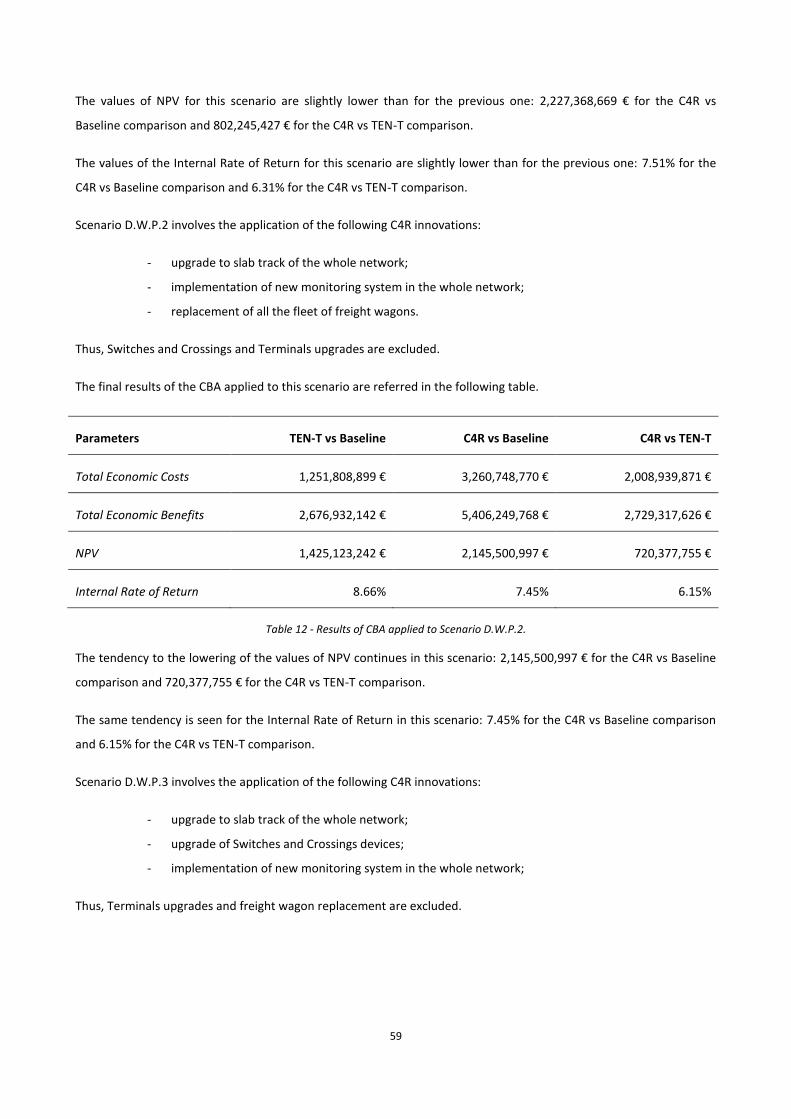
59
The values of NPV for this scenario are slightly lower than for the previous one: 2,227,368,669 € for the C4R vs
Baseline comparison and 802,245,427 € for the C4R vs TEN-T comparison.
The values of the Internal Rate of Return for this scenario are slightly lower than for the previous one: 7.51% for the
C4R vs Baseline comparison and 6.31% for the C4R vs TEN-T comparison.
Scenario D.W.P.2 involves the application of the following C4R innovations:
- upgrade to slab track of the whole network;
- implementation of new monitoring system in the whole network;
- replacement of all the fleet of freight wagons.
Thus, Switches and Crossings and Terminals upgrades are excluded.
The final results of the CBA applied to this scenario are referred in the following table.
Parameters TEN-T vs Baseline C4R vs Baseline C4R vs TEN-T
Total Economic Costs 1,251,808,899 € 3,260,748,770 € 2,008,939,871 €
Total Economic Benefits 2,676,932,142 € 5,406,249,768 € 2,729,317,626 €
NPV 1,425,123,242 € 2,145,500,997 € 720,377,755 €
Internal Rate of Return 8.66% 7.45% 6.15%
Table 12 - Results of CBA applied to Scenario D.W.P.2.
The tendency to the lowering of the values of NPV continues in this scenario: 2,145,500,997 € for the C4R vs Baseline
comparison and 720,377,755 € for the C4R vs TEN-T comparison.
The same tendency is seen for the Internal Rate of Return in this scenario: 7.45% for the C4R vs Baseline comparison
and 6.15% for the C4R vs TEN-T comparison.
Scenario D.W.P.3 involves the application of the following C4R innovations:
- upgrade to slab track of the whole network;
- upgrade of Switches and Crossings devices;
- implementation of new monitoring system in the whole network;
Thus, Terminals upgrades and freight wagon replacement are excluded.
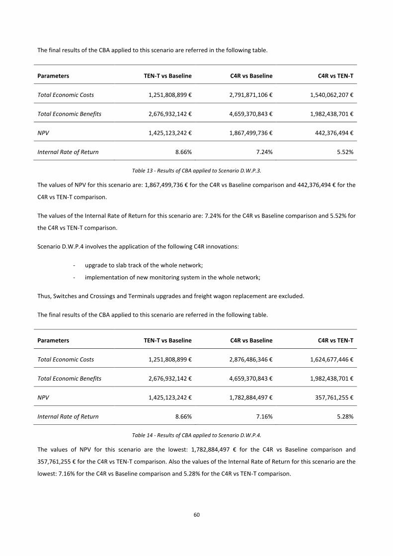
60
The final results of the CBA applied to this scenario are referred in the following table.
Parameters TEN-T vs Baseline C4R vs Baseline C4R vs TEN-T
Total Economic Costs 1,251,808,899 € 2,791,871,106 € 1,540,062,207 €
Total Economic Benefits 2,676,932,142 € 4,659,370,843 € 1,982,438,701 €
NPV 1,425,123,242 € 1,867,499,736 € 442,376,494 €
Internal Rate of Return 8.66% 7.24% 5.52%
Table 13 - Results of CBA applied to Scenario D.W.P.3.
The values of NPV for this scenario are: 1,867,499,736 € for the C4R vs Baseline comparison and 442,376,494 € for the
C4R vs TEN-T comparison.
The values of the Internal Rate of Return for this scenario are: 7.24% for the C4R vs Baseline comparison and 5.52% for
the C4R vs TEN-T comparison.
Scenario D.W.P.4 involves the application of the following C4R innovations:
- upgrade to slab track of the whole network;
- implementation of new monitoring system in the whole network;
Thus, Switches and Crossings and Terminals upgrades and freight wagon replacement are excluded.
The final results of the CBA applied to this scenario are referred in the following table.
Parameters TEN-T vs Baseline C4R vs Baseline C4R vs TEN-T
Total Economic Costs 1,251,808,899 € 2,876,486,346 € 1,624,677,446 €
Total Economic Benefits 2,676,932,142 € 4,659,370,843 € 1,982,438,701 €
NPV 1,425,123,242 € 1,782,884,497 € 357,761,255 €
Internal Rate of Return 8.66% 7.16% 5.28%
Table 14 - Results of CBA applied to Scenario D.W.P.4.
The values of NPV for this scenario are the lowest: 1,782,884,497 € for the C4R vs Baseline comparison and
357,761,255 € for the C4R vs TEN-T comparison. Also the values of the Internal Rate of Return for this scenario are the
lowest: 7.16% for the C4R vs Baseline comparison and 5.28% for the C4R vs TEN-T comparison.
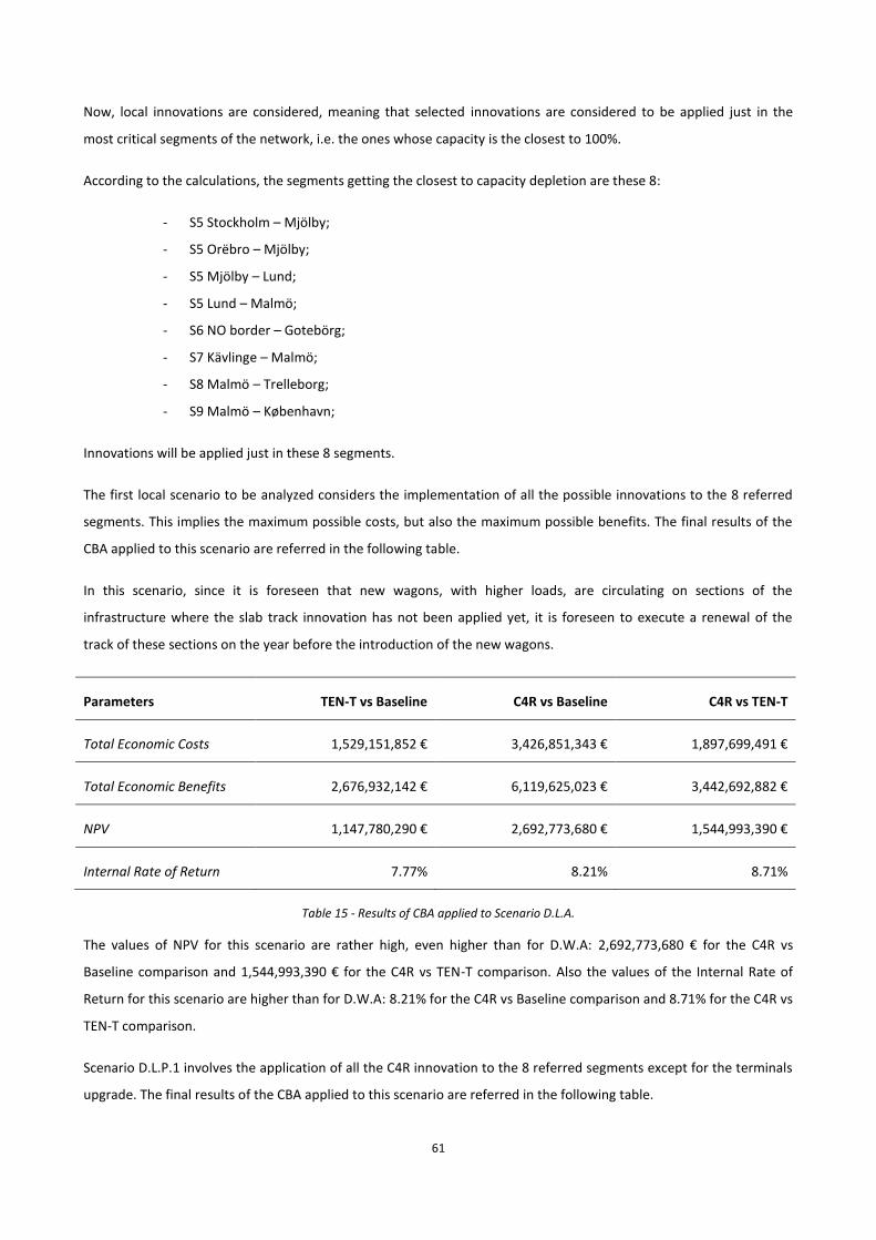
61
Now, local innovations are considered, meaning that selected innovations are considered to be applied just in the
most critical segments of the network, i.e. the ones whose capacity is the closest to 100%.
According to the calculations, the segments getting the closest to capacity depletion are these 8:
- S5 Stockholm – Mjölby;
- S5 Orëbro – Mjölby;
- S5 Mjölby – Lund;
- S5 Lund – Malmö;
- S6 NO border – Gotebörg;
- S7 Kävlinge – Malmö;
- S8 Malmö – Trelleborg;
- S9 Malmö – København;
Innovations will be applied just in these 8 segments.
The first local scenario to be analyzed considers the implementation of all the possible innovations to the 8 referred
segments. This implies the maximum possible costs, but also the maximum possible benefits. The final results of the
CBA applied to this scenario are referred in the following table.
In this scenario, since it is foreseen that new wagons, with higher loads, are circulating on sections of the
infrastructure where the slab track innovation has not been applied yet, it is foreseen to execute a renewal of the
track of these sections on the year before the introduction of the new wagons.
Parameters TEN-T vs Baseline C4R vs Baseline C4R vs TEN-T
Total Economic Costs 1,529,151,852 € 3,426,851,343 € 1,897,699,491 €
Total Economic Benefits 2,676,932,142 € 6,119,625,023 € 3,442,692,882 €
NPV 1,147,780,290 € 2,692,773,680 € 1,544,993,390 €
Internal Rate of Return 7.77% 8.21% 8.71%
Table 15 - Results of CBA applied to Scenario D.L.A.
The values of NPV for this scenario are rather high, even higher than for D.W.A: 2,692,773,680 € for the C4R vs
Baseline comparison and 1,544,993,390 € for the C4R vs TEN-T comparison. Also the values of the Internal Rate of
Return for this scenario are higher than for D.W.A: 8.21% for the C4R vs Baseline comparison and 8.71% for the C4R vs
TEN-T comparison.
Scenario D.L.P.1 involves the application of all the C4R innovation to the 8 referred segments except for the terminals
upgrade. The final results of the CBA applied to this scenario are referred in the following table.
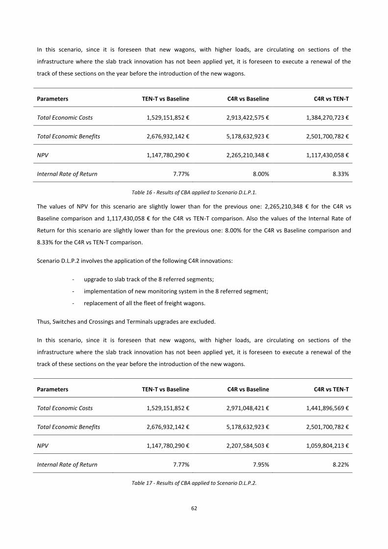
62
In this scenario, since it is foreseen that new wagons, with higher loads, are circulating on sections of the
infrastructure where the slab track innovation has not been applied yet, it is foreseen to execute a renewal of the
track of these sections on the year before the introduction of the new wagons.
Parameters TEN-T vs Baseline C4R vs Baseline C4R vs TEN-T
Total Economic Costs 1,529,151,852 € 2,913,422,575 € 1,384,270,723 €
Total Economic Benefits 2,676,932,142 € 5,178,632,923 € 2,501,700,782 €
NPV 1,147,780,290 € 2,265,210,348 € 1,117,430,058 €
Internal Rate of Return 7.77% 8.00% 8.33%
Table 16 - Results of CBA applied to Scenario D.L.P.1.
The values of NPV for this scenario are slightly lower than for the previous one: 2,265,210,348 € for the C4R vs
Baseline comparison and 1,117,430,058 € for the C4R vs TEN-T comparison. Also the values of the Internal Rate of
Return for this scenario are slightly lower than for the previous one: 8.00% for the C4R vs Baseline comparison and
8.33% for the C4R vs TEN-T comparison.
Scenario D.L.P.2 involves the application of the following C4R innovations:
- upgrade to slab track of the 8 referred segments;
- implementation of new monitoring system in the 8 referred segment;
- replacement of all the fleet of freight wagons.
Thus, Switches and Crossings and Terminals upgrades are excluded.
In this scenario, since it is foreseen that new wagons, with higher loads, are circulating on sections of the
infrastructure where the slab track innovation has not been applied yet, it is foreseen to execute a renewal of the
track of these sections on the year before the introduction of the new wagons.
Parameters TEN-T vs Baseline C4R vs Baseline C4R vs TEN-T
Total Economic Costs 1,529,151,852 € 2,971,048,421 € 1,441,896,569 €
Total Economic Benefits 2,676,932,142 € 5,178,632,923 € 2,501,700,782 €
NPV 1,147,780,290 € 2,207,584,503 € 1,059,804,213 €
Internal Rate of Return 7.77% 7.95% 8.22%
Table 17 - Results of CBA applied to Scenario D.L.P.2.
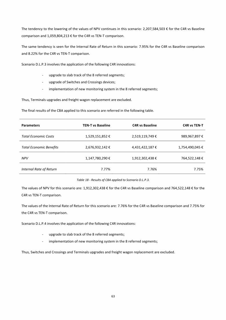
63
The tendency to the lowering of the values of NPV continues in this scenario: 2,207,584,503 € for the C4R vs Baseline
comparison and 1,059,804,213 € for the C4R vs TEN-T comparison.
The same tendency is seen for the Internal Rate of Return in this scenario: 7.95% for the C4R vs Baseline comparison
and 8.22% for the C4R vs TEN-T comparison.
Scenario D.L.P.3 involves the application of the following C4R innovations:
- upgrade to slab track of the 8 referred segments;
- upgrade of Switches and Crossings devices;
- implementation of new monitoring system in the 8 referred segments;
Thus, Terminals upgrades and freight wagon replacement are excluded.
The final results of the CBA applied to this scenario are referred in the following table.
Parameters TEN-T vs Baseline C4R vs Baseline C4R vs TEN-T
Total Economic Costs 1,529,151,852 € 2,519,119,749 € 989,967,897 €
Total Economic Benefits 2,676,932,142 € 4,431,422,187 € 1,754,490,045 €
NPV 1,147,780,290 € 1,912,302,438 € 764,522,148 €
Internal Rate of Return 7.77% 7.76% 7.75%
Table 18 - Results of CBA applied to Scenario D.L.P.3.
The values of NPV for this scenario are: 1,912,302,438 € for the C4R vs Baseline comparison and 764,522,148 € for the
C4R vs TEN-T comparison.
The values of the Internal Rate of Return for this scenario are: 7.76% for the C4R vs Baseline comparison and 7.75% for
the C4R vs TEN-T comparison.
Scenario D.L.P.4 involves the application of the following C4R innovations:
- upgrade to slab track of the 8 referred segments;
- implementation of new monitoring system in the 8 referred segments;
Thus, Switches and Crossings and Terminals upgrades and freight wagon replacement are excluded.
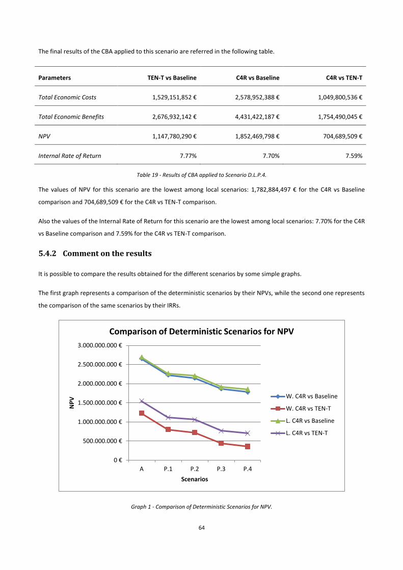
64
The final results of the CBA applied to this scenario are referred in the following table.
Parameters TEN-T vs Baseline C4R vs Baseline C4R vs TEN-T
Total Economic Costs 1,529,151,852 € 2,578,952,388 € 1,049,800,536 €
Total Economic Benefits 2,676,932,142 € 4,431,422,187 € 1,754,490,045 €
NPV 1,147,780,290 € 1,852,469,798 € 704,689,509 €
Internal Rate of Return 7.77% 7.70% 7.59%
Table 19 - Results of CBA applied to Scenario D.L.P.4.
The values of NPV for this scenario are the lowest among local scenarios: 1,782,884,497 € for the C4R vs Baseline
comparison and 704,689,509 € for the C4R vs TEN-T comparison.
Also the values of the Internal Rate of Return for this scenario are the lowest among local scenarios: 7.70% for the C4R
vs Baseline comparison and 7.59% for the C4R vs TEN-T comparison.
5.4.2 Comment on the results
It is possible to compare the results obtained for the different scenarios by some simple graphs.
The first graph represents a comparison of the deterministic scenarios by their NPVs, while the second one represents
the comparison of the same scenarios by their IRRs.
Graph 1 - Comparison of Deterministic Scenarios for NPV.
0 €
500.000.000 €
1.000.000.000 €
1.500.000.000 €
2.000.000.000 €
2.500.000.000 €
3.000.000.000 €
A P.1 P.2 P.3 P.4
NP
V
Scenarios
Comparison of Deterministic Scenarios for NPV
W. C4R vs Baseline
W. C4R vs TEN-T
L. C4R vs Baseline
L. C4R vs TEN-T
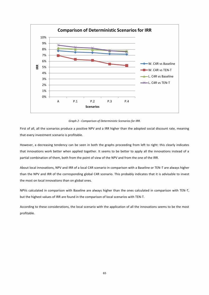
65
Graph 2 - Comparison of Deterministic Scenarios for IRR.
First of all, all the scenarios produce a positive NPV and a IRR higher than the adopted social discount rate, meaning
that every investment scenario is profitable.
However, a decreasing tendency can be seen in both the graphs proceeding from left to right: this clearly indicates
that innovations work better when applied together. It seems to be better to apply all the innovations instead of a
partial combination of them, both from the point of view of the NPV and from the one of the IRR.
About local innovations, NPV and IRR of a local C4R scenario in comparison with a Baseline or TEN-T are always higher
than the NPV and IRR of the corresponding global C4R scenario. This probably indicates that it is advisable to invest
the most on local innovations than on global ones.
NPVs calculated in comparison with Baseline are always higher than the ones calculated in comparison with TEN-T,
but the highest values of IRR are found in the comparison of local scenarios with TEN-T.
According to these considerations, the local scenario with the application of all the innovations seems to be the most
profitable.
0%
1%
2%
3%
4%
5%
6%
7%
8%
9%
10%
A P.1 P.2 P.3 P.4
IRR
Scenarios
Comparison of Deterministic Scenarios for IRR
W. C4R vs Baseline
W. C4R vs TEN-T
L. C4R vs Baseline
L. C4R vs TEN-T
66
5.5 Sensitivity analysis
After the deterministic analysis, a sensitivity analysis was performed in order to find out which are the critical
variables of the present analysis.
The individuation of the critical variables was carried out through the method suggested in the EU guidelines: as it was
already referred in paragraph 3.2.7.1, the recommendation is to consider critical those variables for which a variation
of ± 1% of the value adopted in the base case gives rise to a variation greater than 1% in the final value of NPV.
Once again, the special character and the complexity of the analysis are displayed in this step. The “base case” of the
present analysis is indeed given by 10 different scenarios, thus, considering all of them, an enormous number of
calculation would be executed.
Therefore, for the determination of the critical variables, just scenario D.W.A was considered, which is also the
scenario giving the best results in terms of economic performance.
EU guidelines recommend to test at least the following variables, being the ones that usually have the biggest
influence on NPV:
value of time;
accident costs;
assumptions on GDP and other economic variables trend;
rate of increase of traffic over time;
number of years necessary for the realization of the infrastructure;
investment and maintenance costs (as disaggregated as possible);
fare/tariff/toll.
In the present case, accidents are not considered, the realization time of the innovations is considered in a simplified
way being always considered equal to 1 year and fares are not considered, because transferences of money from one
agent to another one are left out of the analysis for the moment.
All the other variables in the list are analyzed, together with many others. The variable not showing any variation from
TEN-T to C4R scenarios were excluded from the sensitivity analysis.
The calculation leading to the determination of the critical variables are summarized in the table in ANNEX 1. For each
considered variable, both the variation imposed to the input, amounting to ± 1%, and the corresponding variation in
the final values of NPVs are displayed. The variables for which this variation is greater than 1 % are then highlighted
and considered as critical variables.
Summarizing the results, these were found out to be the critical variables of the present case:
Social discount rate;
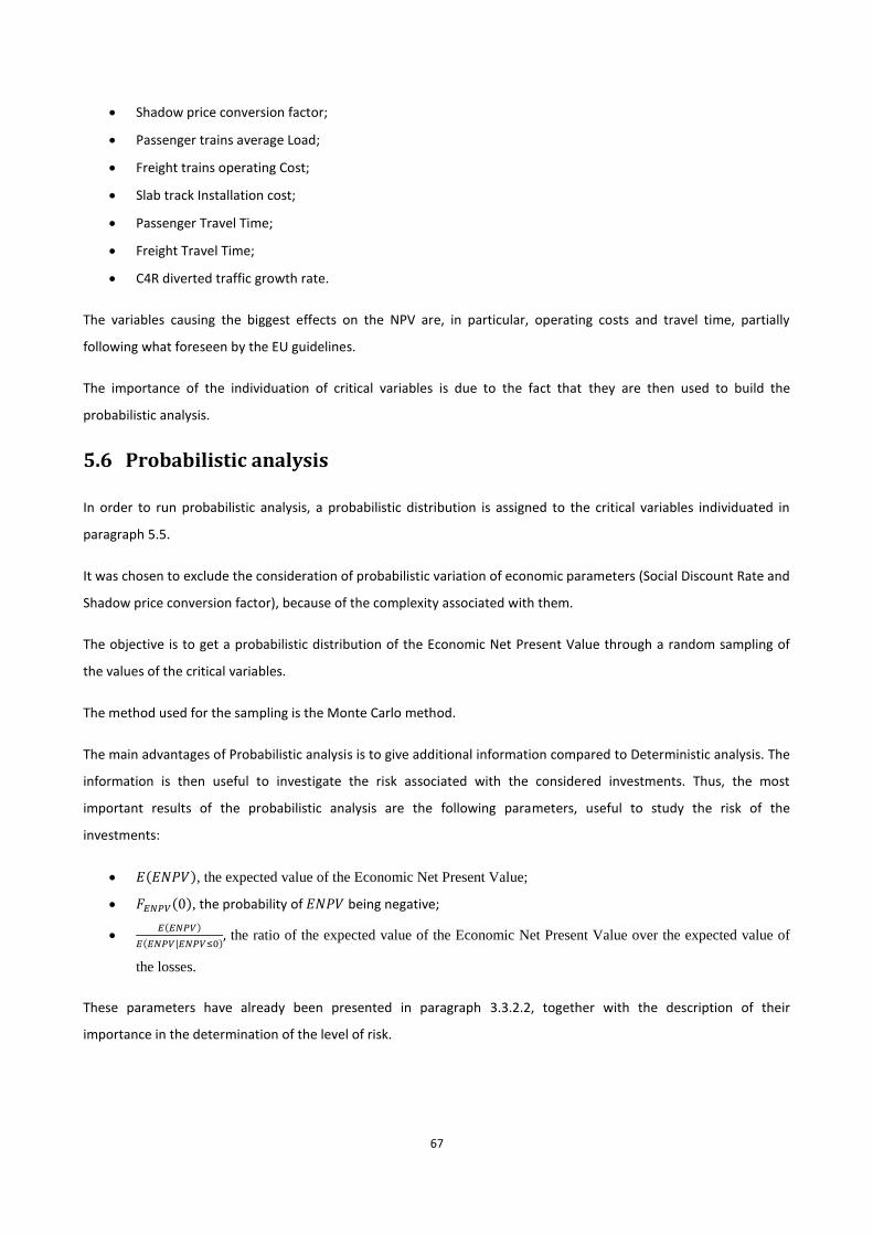
67
Shadow price conversion factor;
Passenger trains average Load;
Freight trains operating Cost;
Slab track Installation cost;
Passenger Travel Time;
Freight Travel Time;
C4R diverted traffic growth rate.
The variables causing the biggest effects on the NPV are, in particular, operating costs and travel time, partially
following what foreseen by the EU guidelines.
The importance of the individuation of critical variables is due to the fact that they are then used to build the
probabilistic analysis.
5.6 Probabilistic analysis
In order to run probabilistic analysis, a probabilistic distribution is assigned to the critical variables individuated in
paragraph 5.5.
It was chosen to exclude the consideration of probabilistic variation of economic parameters (Social Discount Rate and
Shadow price conversion factor), because of the complexity associated with them.
The objective is to get a probabilistic distribution of the Economic Net Present Value through a random sampling of
the values of the critical variables.
The method used for the sampling is the Monte Carlo method.
The main advantages of Probabilistic analysis is to give additional information compared to Deterministic analysis. The
information is then useful to investigate the risk associated with the considered investments. Thus, the most
important results of the probabilistic analysis are the following parameters, useful to study the risk of the
investments:
𝐸(𝐸𝑁𝑃𝑉), the expected value of the Economic Net Present Value;
𝐹𝐸𝑁𝑃𝑉(0), the probability of 𝐸𝑁𝑃𝑉 being negative;
𝐸(𝐸𝑁𝑃𝑉)
𝐸(𝐸𝑁𝑃𝑉|𝐸𝑁𝑃𝑉≤0), the ratio of the expected value of the Economic Net Present Value over the expected value of
the losses.
These parameters have already been presented in paragraph 3.3.2.2, together with the description of their
importance in the determination of the level of risk.

68
5.6.1 Critical variables distributions
It was chosen to run the probabilistic analysis considering a Normal distribution for each of the critical variables,
having the original value of the variable as average value and variance equal to 10% of the average value.
The definition of the adopted distributions is contained in the following table.
Critical Variable Type of distribution Mean Value Standard deviation
Freight Train Operating cost [€/T·km] Normal 0.0288 0.00288
Slab Track Installation cost [€/km] Normal 1,000,000 100,000
Passenger Trains Journey Time [h] Normal Deterministic Value 0.1·Deterministic Value
Freight Trains Journey Time [h] Normal Deterministic Value 0.1·Deterministic Value
Div. Traffic Growth rate 2025 – 2030 Normal 6% 0,6%
Table 20 - Definition of the adopted distributions for the critical variables considered for the Probabilistic Analysis.
5.6.2 Discussion about the number of iterations
In order to choose the number of iterations to run the probabilistic analysis, a convergence analysis was executed,
considering the P.W.A. scenario with 1,000, 2,000, 5,000 and 10,000 iterations. Each number of iterations was tested
5 times. The results, both for C4R vs Baseline mean NPV and C4R vs TEN-T mean NPV, are shown in the following
graphs:
Graph 3 - Convergence analysis considering C4R vs Baseline NPV mean value.
2,48E+09
2,5E+09
2,52E+09
2,54E+09
2,56E+09
2,58E+09
2,6E+09
2,62E+09
0 2000 4000 6000 8000 10000 12000Me
an o
f N
PV
of
C4
R v
s B
ase
line
[€
]
Number of iterations
Convergence analysis - C4R vs Baseline
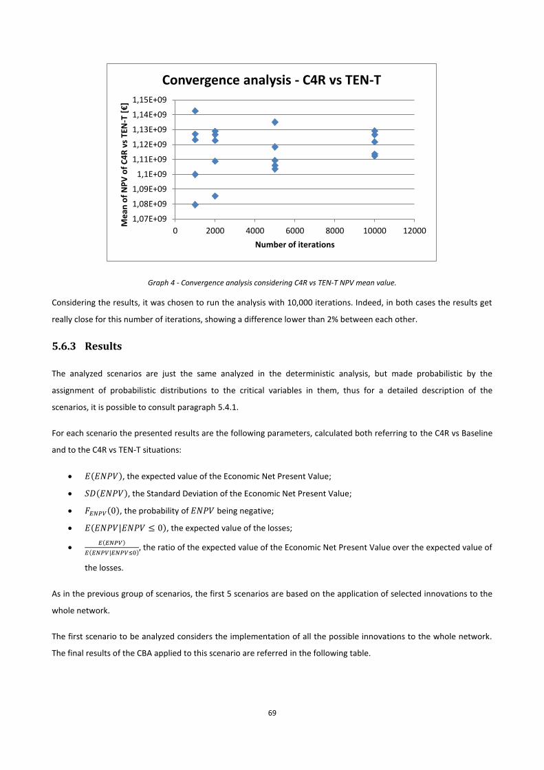
69
Graph 4 - Convergence analysis considering C4R vs TEN-T NPV mean value.
Considering the results, it was chosen to run the analysis with 10,000 iterations. Indeed, in both cases the results get
really close for this number of iterations, showing a difference lower than 2% between each other.
5.6.3 Results
The analyzed scenarios are just the same analyzed in the deterministic analysis, but made probabilistic by the
assignment of probabilistic distributions to the critical variables in them, thus for a detailed description of the
scenarios, it is possible to consult paragraph 5.4.1.
For each scenario the presented results are the following parameters, calculated both referring to the C4R vs Baseline
and to the C4R vs TEN-T situations:
𝐸(𝐸𝑁𝑃𝑉), the expected value of the Economic Net Present Value;
𝑆𝐷(𝐸𝑁𝑃𝑉), the Standard Deviation of the Economic Net Present Value;
𝐹𝐸𝑁𝑃𝑉(0), the probability of 𝐸𝑁𝑃𝑉 being negative;
𝐸(𝐸𝑁𝑃𝑉|𝐸𝑁𝑃𝑉 ≤ 0), the expected value of the losses;
𝐸(𝐸𝑁𝑃𝑉)
𝐸(𝐸𝑁𝑃𝑉|𝐸𝑁𝑃𝑉≤0), the ratio of the expected value of the Economic Net Present Value over the expected value of
the losses.
As in the previous group of scenarios, the first 5 scenarios are based on the application of selected innovations to the
whole network.
The first scenario to be analyzed considers the implementation of all the possible innovations to the whole network.
The final results of the CBA applied to this scenario are referred in the following table.
1,07E+09
1,08E+09
1,09E+09
1,1E+09
1,11E+09
1,12E+09
1,13E+09
1,14E+09
1,15E+09
0 2000 4000 6000 8000 10000 12000
Me
an o
f N
PV
of
C4
R v
s TE
N-T
[€
]
Number of iterations
Convergence analysis - C4R vs TEN-T
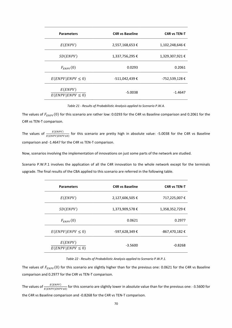
70
Parameters C4R vs Baseline C4R vs TEN-T
𝐸(𝐸𝑁𝑃𝑉) 2,557,168,653 € 1,102,248,646 €
𝑆𝐷(𝐸𝑁𝑃𝑉) 1,337,756,295 € 1,329,307,921 €
𝐹𝐸𝑁𝑃𝑉(0) 0.0293 0.2061
𝐸(𝐸𝑁𝑃𝑉|𝐸𝑁𝑃𝑉 ≤ 0) -511,042,439 € -752,539,128 €
𝐸(𝐸𝑁𝑃𝑉)
𝐸(𝐸𝑁𝑃𝑉|𝐸𝑁𝑃𝑉 ≤ 0) -5.0038 -1.4647
Table 21 - Results of Probabilistic Analysis applied to Scenario P.W.A.
The values of 𝐹𝐸𝑁𝑃𝑉(0) for this scenario are rather low: 0.0293 for the C4R vs Baseline comparison and 0.2061 for the
C4R vs TEN-T comparison.
The values of 𝐸(𝐸𝑁𝑃𝑉)
𝐸(𝐸𝑁𝑃𝑉|𝐸𝑁𝑃𝑉≤0) for this scenario are pretty high in absolute value: -5.0038 for the C4R vs Baseline
comparison and -1.4647 for the C4R vs TEN-T comparison.
Now, scenarios involving the implementation of innovations on just some parts of the network are studied.
Scenario P.W.P.1 involves the application of all the C4R innovation to the whole network except for the terminals
upgrade. The final results of the CBA applied to this scenario are referred in the following table.
Parameters C4R vs Baseline C4R vs TEN-T
𝐸(𝐸𝑁𝑃𝑉) 2,127,606,505 € 717,225,007 €
𝑆𝐷(𝐸𝑁𝑃𝑉) 1,373,909,578 € 1,358,352,729 €
𝐹𝐸𝑁𝑃𝑉(0) 0.0621 0.2977
𝐸(𝐸𝑁𝑃𝑉|𝐸𝑁𝑃𝑉 ≤ 0) -597,628,349 € -867,470,182 €
𝐸(𝐸𝑁𝑃𝑉)
𝐸(𝐸𝑁𝑃𝑉|𝐸𝑁𝑃𝑉 ≤ 0) -3.5600 -0.8268
Table 22 - Results of Probabilistic Analysis applied to Scenario P.W.P.1.
The values of 𝐹𝐸𝑁𝑃𝑉(0) for this scenario are slightly higher than for the previous one: 0.0621 for the C4R vs Baseline
comparison and 0.2977 for the C4R vs TEN-T comparison.
The values of 𝐸(𝐸𝑁𝑃𝑉)
𝐸(𝐸𝑁𝑃𝑉|𝐸𝑁𝑃𝑉≤0) for this scenario are slightly lower in absolute value than for the previous one: -3.5600 for
the C4R vs Baseline comparison and -0.8268 for the C4R vs TEN-T comparison.
71
Scenario P.W.P.2 involves the application of all the C4R innovation to the whole network except for Switches and
Crossings and Terminals upgrades.
The final results of the CBA applied to this scenario are referred in the following table.
Parameters C4R vs Baseline C4R vs TEN-T
𝐸(𝐸𝑁𝑃𝑉) 2,041,748,985 € 623,027,018 €
𝑆𝐷(𝐸𝑁𝑃𝑉) 1,369,941,468 € 1,370,747,607 €
𝐹𝐸𝑁𝑃𝑉(0) 0.0672 0.3258
𝐸(𝐸𝑁𝑃𝑉|𝐸𝑁𝑃𝑉 ≤ 0) -640,977,191 € -901,250,184 €
𝐸(𝐸𝑁𝑃𝑉)
𝐸(𝐸𝑁𝑃𝑉|𝐸𝑁𝑃𝑉 ≤ 0) -3.1853 -0.6912
Table 23 - Results of Probabilistic Analysis applied to Scenario P.W.P.2.
The tendency to the increasing of the values of 𝐹𝐸𝑁𝑃𝑉(0) continues in this scenario: 0.0672 for the C4R vs Baseline
comparison and 0.3258 for the C4R vs TEN-T comparison.
The opposite tendency is seen for absolute values of 𝐸(𝐸𝑁𝑃𝑉)
𝐸(𝐸𝑁𝑃𝑉|𝐸𝑁𝑃𝑉≤0) in this scenario: -3.1853 for the C4R vs Baseline
comparison and -0.6912 for the C4R vs TEN-T comparison.
Scenario P.W.P.3 involves the application of all the C4R innovation to the whole network except for Terminals
upgrades and freight wagon replacement.
The final results of the CBA applied to this scenario are referred in the following table.
Parameters C4R vs Baseline C4R vs TEN-T
𝐸(𝐸𝑁𝑃𝑉) 1,750,494,170 € 329,721,494 €
𝑆𝐷(𝐸𝑁𝑃𝑉) 1,218,083,354 € 1,228,428,048 €
𝐹𝐸𝑁𝑃𝑉(0) 0.0761 0.3878
𝐸(𝐸𝑁𝑃𝑉|𝐸𝑁𝑃𝑉 ≤ 0) -531,948,130 € -888,059,361 €
𝐸(𝐸𝑁𝑃𝑉)
𝐸(𝐸𝑁𝑃𝑉|𝐸𝑁𝑃𝑉 ≤ 0) -3.2907 -0.3712
Table 24 - Results of Probabilistic Analysis applied to Scenario P.W.P.3.
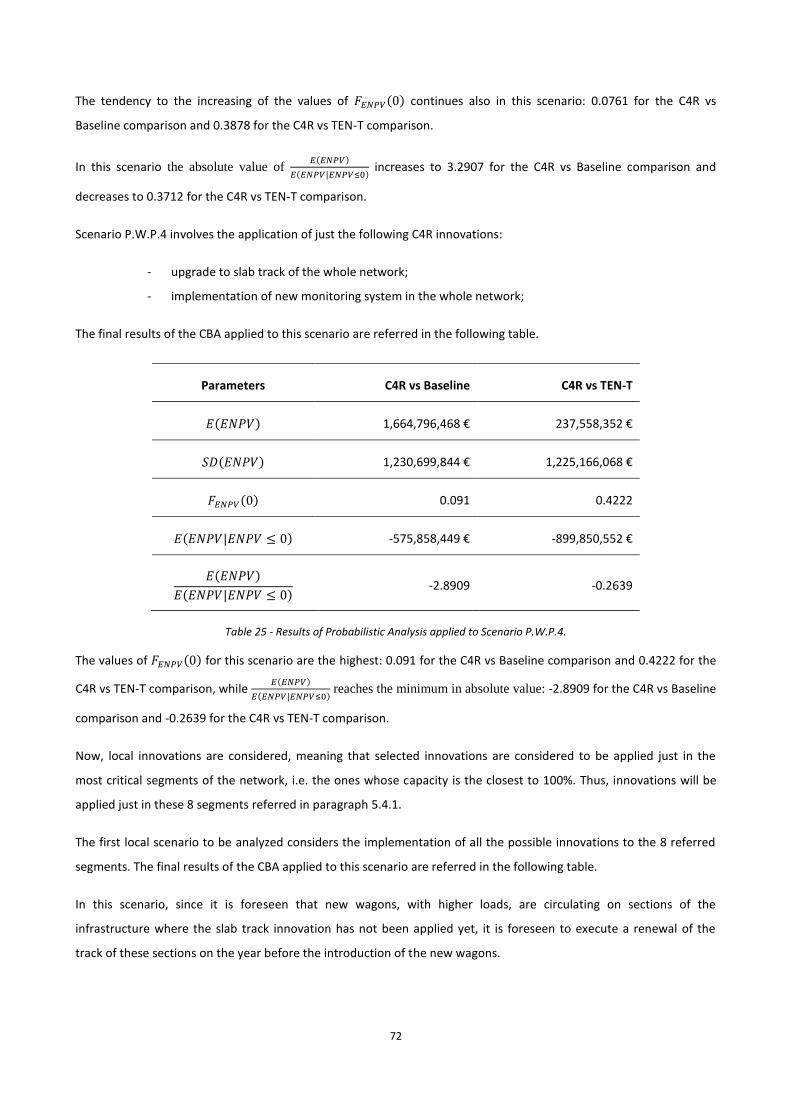
72
The tendency to the increasing of the values of 𝐹𝐸𝑁𝑃𝑉(0) continues also in this scenario: 0.0761 for the C4R vs
Baseline comparison and 0.3878 for the C4R vs TEN-T comparison.
In this scenario the absolute value of 𝐸(𝐸𝑁𝑃𝑉)
𝐸(𝐸𝑁𝑃𝑉|𝐸𝑁𝑃𝑉≤0) increases to 3.2907 for the C4R vs Baseline comparison and
decreases to 0.3712 for the C4R vs TEN-T comparison.
Scenario P.W.P.4 involves the application of just the following C4R innovations:
- upgrade to slab track of the whole network;
- implementation of new monitoring system in the whole network;
The final results of the CBA applied to this scenario are referred in the following table.
Parameters C4R vs Baseline C4R vs TEN-T
𝐸(𝐸𝑁𝑃𝑉) 1,664,796,468 € 237,558,352 €
𝑆𝐷(𝐸𝑁𝑃𝑉) 1,230,699,844 € 1,225,166,068 €
𝐹𝐸𝑁𝑃𝑉(0) 0.091 0.4222
𝐸(𝐸𝑁𝑃𝑉|𝐸𝑁𝑃𝑉 ≤ 0) -575,858,449 € -899,850,552 €
𝐸(𝐸𝑁𝑃𝑉)
𝐸(𝐸𝑁𝑃𝑉|𝐸𝑁𝑃𝑉 ≤ 0) -2.8909 -0.2639
Table 25 - Results of Probabilistic Analysis applied to Scenario P.W.P.4.
The values of 𝐹𝐸𝑁𝑃𝑉(0) for this scenario are the highest: 0.091 for the C4R vs Baseline comparison and 0.4222 for the
C4R vs TEN-T comparison, while 𝐸(𝐸𝑁𝑃𝑉)
𝐸(𝐸𝑁𝑃𝑉|𝐸𝑁𝑃𝑉≤0) reaches the minimum in absolute value: -2.8909 for the C4R vs Baseline
comparison and -0.2639 for the C4R vs TEN-T comparison.
Now, local innovations are considered, meaning that selected innovations are considered to be applied just in the
most critical segments of the network, i.e. the ones whose capacity is the closest to 100%. Thus, innovations will be
applied just in these 8 segments referred in paragraph 5.4.1.
The first local scenario to be analyzed considers the implementation of all the possible innovations to the 8 referred
segments. The final results of the CBA applied to this scenario are referred in the following table.
In this scenario, since it is foreseen that new wagons, with higher loads, are circulating on sections of the
infrastructure where the slab track innovation has not been applied yet, it is foreseen to execute a renewal of the
track of these sections on the year before the introduction of the new wagons.
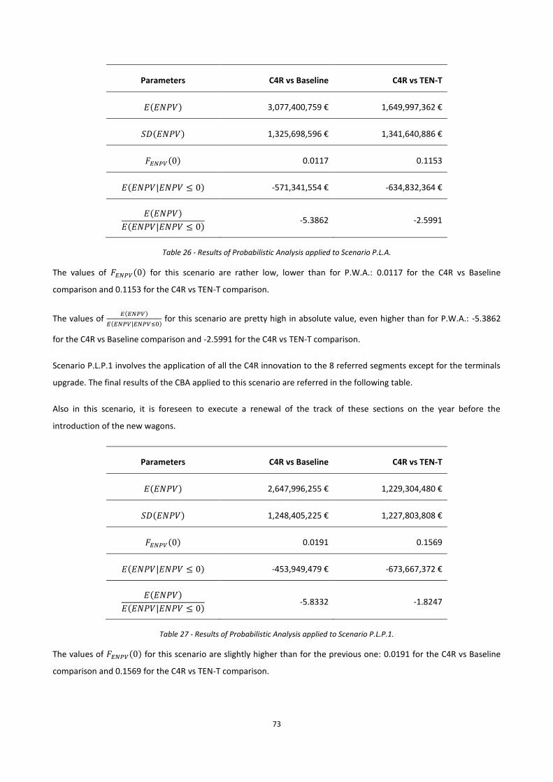
73
Parameters C4R vs Baseline C4R vs TEN-T
𝐸(𝐸𝑁𝑃𝑉) 3,077,400,759 € 1,649,997,362 €
𝑆𝐷(𝐸𝑁𝑃𝑉) 1,325,698,596 € 1,341,640,886 €
𝐹𝐸𝑁𝑃𝑉(0) 0.0117 0.1153
𝐸(𝐸𝑁𝑃𝑉|𝐸𝑁𝑃𝑉 ≤ 0) -571,341,554 € -634,832,364 €
𝐸(𝐸𝑁𝑃𝑉)
𝐸(𝐸𝑁𝑃𝑉|𝐸𝑁𝑃𝑉 ≤ 0) -5.3862 -2.5991
Table 26 - Results of Probabilistic Analysis applied to Scenario P.L.A.
The values of 𝐹𝐸𝑁𝑃𝑉(0) for this scenario are rather low, lower than for P.W.A.: 0.0117 for the C4R vs Baseline
comparison and 0.1153 for the C4R vs TEN-T comparison.
The values of 𝐸(𝐸𝑁𝑃𝑉)
𝐸(𝐸𝑁𝑃𝑉|𝐸𝑁𝑃𝑉≤0) for this scenario are pretty high in absolute value, even higher than for P.W.A.: -5.3862
for the C4R vs Baseline comparison and -2.5991 for the C4R vs TEN-T comparison.
Scenario P.L.P.1 involves the application of all the C4R innovation to the 8 referred segments except for the terminals
upgrade. The final results of the CBA applied to this scenario are referred in the following table.
Also in this scenario, it is foreseen to execute a renewal of the track of these sections on the year before the
introduction of the new wagons.
Parameters C4R vs Baseline C4R vs TEN-T
𝐸(𝐸𝑁𝑃𝑉) 2,647,996,255 € 1,229,304,480 €
𝑆𝐷(𝐸𝑁𝑃𝑉) 1,248,405,225 € 1,227,803,808 €
𝐹𝐸𝑁𝑃𝑉(0) 0.0191 0.1569
𝐸(𝐸𝑁𝑃𝑉|𝐸𝑁𝑃𝑉 ≤ 0) -453,949,479 € -673,667,372 €
𝐸(𝐸𝑁𝑃𝑉)
𝐸(𝐸𝑁𝑃𝑉|𝐸𝑁𝑃𝑉 ≤ 0) -5.8332 -1.8247
Table 27 - Results of Probabilistic Analysis applied to Scenario P.L.P.1.
The values of 𝐹𝐸𝑁𝑃𝑉(0) for this scenario are slightly higher than for the previous one: 0.0191 for the C4R vs Baseline
comparison and 0.1569 for the C4R vs TEN-T comparison.
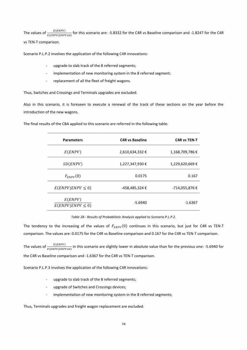
74
The values of 𝐸(𝐸𝑁𝑃𝑉)
𝐸(𝐸𝑁𝑃𝑉|𝐸𝑁𝑃𝑉≤0) for this scenario are: -5.8332 for the C4R vs Baseline comparison and -1.8247 for the C4R
vs TEN-T comparison.
Scenario P.L.P.2 involves the application of the following C4R innovations:
- upgrade to slab track of the 8 referred segments;
- implementation of new monitoring system in the 8 referred segment;
- replacement of all the fleet of freight wagons.
Thus, Switches and Crossings and Terminals upgrades are excluded.
Also in this scenario, it is foreseen to execute a renewal of the track of these sections on the year before the
introduction of the new wagons.
The final results of the CBA applied to this scenario are referred in the following table.
Parameters C4R vs Baseline C4R vs TEN-T
𝐸(𝐸𝑁𝑃𝑉) 2,610,634,332 € 1,168,709,786 €
𝑆𝐷(𝐸𝑁𝑃𝑉) 1,227,347,930 € 1,229,620,669 €
𝐹𝐸𝑁𝑃𝑉(0) 0.0175 0.167
𝐸(𝐸𝑁𝑃𝑉|𝐸𝑁𝑃𝑉 ≤ 0) -458,485,324 € -714,055,876 €
𝐸(𝐸𝑁𝑃𝑉)
𝐸(𝐸𝑁𝑃𝑉|𝐸𝑁𝑃𝑉 ≤ 0) -5.6940 -1.6367
Table 28 - Results of Probabilistic Analysis applied to Scenario P.L.P.2.
The tendency to the increasing of the values of 𝐹𝐸𝑁𝑃𝑉(0) continues in this scenario, but just for C4R vs TEN-T
comparison. The values are: 0.0175 for the C4R vs Baseline comparison and 0.167 for the C4R vs TEN-T comparison.
The values of 𝐸(𝐸𝑁𝑃𝑉)
𝐸(𝐸𝑁𝑃𝑉|𝐸𝑁𝑃𝑉≤0) in this scenario are slightly lower in absolute value than for the previous one: -5.6940 for
the C4R vs Baseline comparison and -1.6367 for the C4R vs TEN-T comparison.
Scenario P.L.P.3 involves the application of the following C4R innovations:
- upgrade to slab track of the 8 referred segments;
- upgrade of Switches and Crossings devices;
- implementation of new monitoring system in the 8 referred segments;
Thus, Terminals upgrades and freight wagon replacement are excluded.
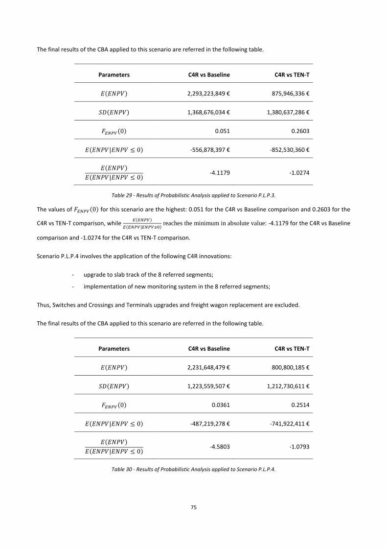
75
The final results of the CBA applied to this scenario are referred in the following table.
Parameters C4R vs Baseline C4R vs TEN-T
𝐸(𝐸𝑁𝑃𝑉) 2,293,223,849 € 875,946,336 €
𝑆𝐷(𝐸𝑁𝑃𝑉) 1,368,676,034 € 1,380,637,286 €
𝐹𝐸𝑁𝑃𝑉(0) 0.051 0.2603
𝐸(𝐸𝑁𝑃𝑉|𝐸𝑁𝑃𝑉 ≤ 0) -556,878,397 € -852,530,360 €
𝐸(𝐸𝑁𝑃𝑉)
𝐸(𝐸𝑁𝑃𝑉|𝐸𝑁𝑃𝑉 ≤ 0) -4.1179 -1.0274
Table 29 - Results of Probabilistic Analysis applied to Scenario P.L.P.3.
The values of 𝐹𝐸𝑁𝑃𝑉(0) for this scenario are the highest: 0.051 for the C4R vs Baseline comparison and 0.2603 for the
C4R vs TEN-T comparison, while 𝐸(𝐸𝑁𝑃𝑉)
𝐸(𝐸𝑁𝑃𝑉|𝐸𝑁𝑃𝑉≤0) reaches the minimum in absolute value: -4.1179 for the C4R vs Baseline
comparison and -1.0274 for the C4R vs TEN-T comparison.
Scenario P.L.P.4 involves the application of the following C4R innovations:
- upgrade to slab track of the 8 referred segments;
- implementation of new monitoring system in the 8 referred segments;
Thus, Switches and Crossings and Terminals upgrades and freight wagon replacement are excluded.
The final results of the CBA applied to this scenario are referred in the following table.
Parameters C4R vs Baseline C4R vs TEN-T
𝐸(𝐸𝑁𝑃𝑉) 2,231,648,479 € 800,800,185 €
𝑆𝐷(𝐸𝑁𝑃𝑉) 1,223,559,507 € 1,212,730,611 €
𝐹𝐸𝑁𝑃𝑉(0) 0.0361 0.2514
𝐸(𝐸𝑁𝑃𝑉|𝐸𝑁𝑃𝑉 ≤ 0) -487,219,278 € -741,922,411 €
𝐸(𝐸𝑁𝑃𝑉)
𝐸(𝐸𝑁𝑃𝑉|𝐸𝑁𝑃𝑉 ≤ 0) -4.5803 -1.0793
Table 30 - Results of Probabilistic Analysis applied to Scenario P.L.P.4.
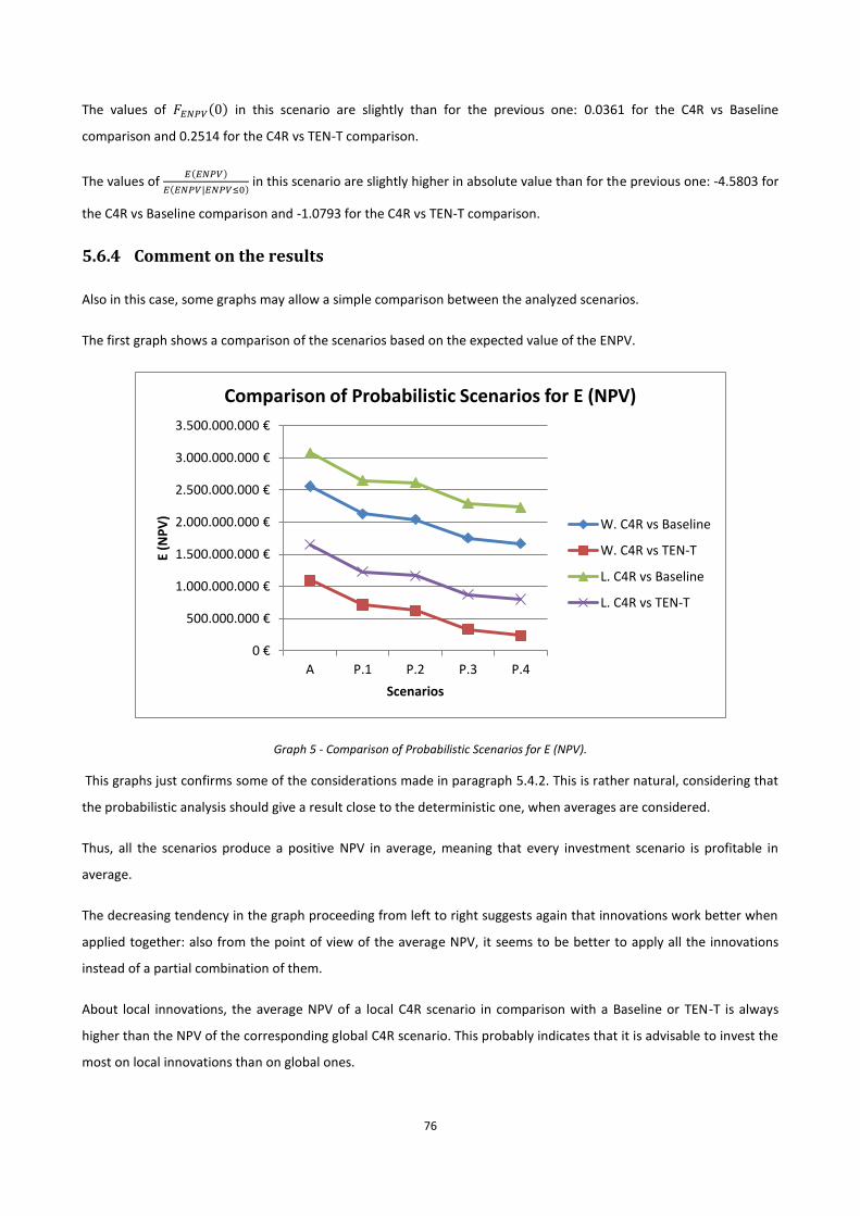
76
The values of 𝐹𝐸𝑁𝑃𝑉(0) in this scenario are slightly than for the previous one: 0.0361 for the C4R vs Baseline
comparison and 0.2514 for the C4R vs TEN-T comparison.
The values of 𝐸(𝐸𝑁𝑃𝑉)
𝐸(𝐸𝑁𝑃𝑉|𝐸𝑁𝑃𝑉≤0) in this scenario are slightly higher in absolute value than for the previous one: -4.5803 for
the C4R vs Baseline comparison and -1.0793 for the C4R vs TEN-T comparison.
5.6.4 Comment on the results
Also in this case, some graphs may allow a simple comparison between the analyzed scenarios.
The first graph shows a comparison of the scenarios based on the expected value of the ENPV.
Graph 5 - Comparison of Probabilistic Scenarios for E (NPV).
This graphs just confirms some of the considerations made in paragraph 5.4.2. This is rather natural, considering that
the probabilistic analysis should give a result close to the deterministic one, when averages are considered.
Thus, all the scenarios produce a positive NPV in average, meaning that every investment scenario is profitable in
average.
The decreasing tendency in the graph proceeding from left to right suggests again that innovations work better when
applied together: also from the point of view of the average NPV, it seems to be better to apply all the innovations
instead of a partial combination of them.
About local innovations, the average NPV of a local C4R scenario in comparison with a Baseline or TEN-T is always
higher than the NPV of the corresponding global C4R scenario. This probably indicates that it is advisable to invest the
most on local innovations than on global ones.
0 €
500.000.000 €
1.000.000.000 €
1.500.000.000 €
2.000.000.000 €
2.500.000.000 €
3.000.000.000 €
3.500.000.000 €
A P.1 P.2 P.3 P.4
E (N
PV
)
Scenarios
Comparison of Probabilistic Scenarios for E (NPV)
W. C4R vs Baseline
W. C4R vs TEN-T
L. C4R vs Baseline
L. C4R vs TEN-T
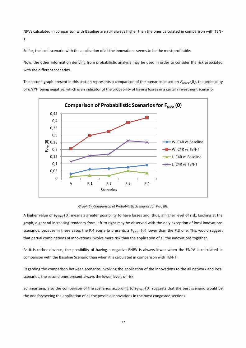
77
NPVs calculated in comparison with Baseline are still always higher than the ones calculated in comparison with TEN-
T.
So far, the local scenario with the application of all the innovations seems to be the most profitable.
Now, the other information deriving from probabilistic analysis may be used in order to consider the risk associated
with the different scenarios.
The second graph present in this section represents a comparison of the scenarios based on 𝐹𝐸𝑁𝑃𝑉(0), the probability
of 𝐸𝑁𝑃𝑉 being negative, which is an indicator of the probability of having losses in a certain investment scenario.
Graph 6 - Comparison of Probabilistic Scenarios for FNPV (0).
A higher value of 𝐹𝐸𝑁𝑃𝑉(0) means a greater possibility to have losses and, thus, a higher level of risk. Looking at the
graph, a general increasing tendency from left to right may be observed with the only exception of local innovations
scenarios, because in these cases the P.4 scenario presents a 𝐹𝐸𝑁𝑃𝑉(0) lower than the P.3 one. This would suggest
that partial combinations of innovations involve more risk than the application of all the innovations together.
As it is rather obvious, the possibility of having a negative ENPV is always lower when the ENPV is calculated in
comparison with the Baseline Scenario than when it is calculated in comparison with TEN-T.
Regarding the comparison between scenarios involving the application of the innovations to the all network and local
scenarios, the second ones present always the lower levels of risk.
Summarizing, also the comparison of the scenarios according to 𝐹𝐸𝑁𝑃𝑉(0) suggests that the best scenario would be
the one foreseeing the application of all the possible innovations in the most congested sections.
0
0,05
0,1
0,15
0,2
0,25
0,3
0,35
0,4
0,45
A P.1 P.2 P.3 P.4
F NP
V(0
)
Scenarios
Comparison of Probabilistic Scenarios for FNPV (0)
W. C4R vs Baseline
W. C4R vs TEN-T
L. C4R vs Baseline
L. C4R vs TEN-T
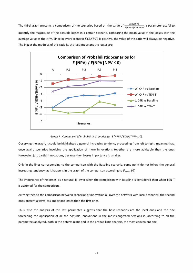
78
The third graph presents a comparison of the scenarios based on the value of 𝐸(𝐸𝑁𝑃𝑉)
𝐸(𝐸𝑁𝑃𝑉|𝐸𝑁𝑃𝑉≤0), a parameter useful to
quantify the magnitude of the possible losses in a certain scenario, comparing the mean value of the losses with the
average value of the NPV. Since in every scenario 𝐸(𝐸𝑁𝑃𝑉) is positive, the value of this ratio will always be negative.
The bigger the modulus of this ratio is, the less important the losses are.
Graph 7 - Comparison of Probabilistic Scenarios for E (NPV) / E(NPV|NPV ≤ 0).
Observing the graph, it could be highlighted a general increasing tendency proceeding from left to right, meaning that,
once again, scenarios involving the application of more innovations together are more advisable than the ones
foreseeing just partial innovations, because their losses importance is smaller.
Only in the lines corresponding to the comparison with the Baseline scenario, some point do not follow the general
increasing tendency, as it happens in the graph of the comparison according to 𝐹𝐸𝑁𝑃𝑉(0).
The importance of the losses, as it natural, is lower when the comparison with Baseline is considered than when TEN-T
is assumed for the comparison.
Arriving then to the comparison between scenarios of innovation all over the network with local scenarios, the second
ones present always less important losses than the first ones.
Thus, also the analysis of this last parameter suggests that the best scenarios are the local ones and the one
foreseeing the application of all the possible innovations in the most congested sections is, according to all the
parameters analyzed, both in the deterministic and in the probabilistic analysis, the most convenient one.
-7
-6
-5
-4
-3
-2
-1
0
A P.1 P.2 P.3 P.4
E (N
PV
) /
E(N
PV
|NP
V ≤
0)
Scenarios
Comparison of Probabilistic Scenarios forE (NPV) / E(NPV|NPV ≤ 0)
W. C4R vs Baseline
W. C4R vs TEN-T
L. C4R vs Baseline
L. C4R vs TEN-T
79
6. CONCLUSIONS
In this last chapter, the conclusions of the work are exposed.
In Chapter 2 the main outlines of European transport policy were presented, highlighting the main objectives of EU
regarding the transport field. The main of these are the reduction of congestion, oil dependency and GHG emissions.
Railways would have a great potential in helping EU to achieve these goals, however European railways are facing
major challenges nowadays: scarcity of capacity, lack of reliability and low travel time competitiveness are the main
ones. That is why many projects are now ongoing, trying to answer these challenges. Among these, TEN-T individuated
the most important railway corridors and the main investments to perform on them, while C4R is developing
technological innovations to be applied on these corridors with the aim of obtaining an affordable, adaptable,
automated, resilient and high-capacity railway.
The global character of these projects implies that normal appraisal tools, usually adopted for projects cannot be used
in these cases. Thus, the challenged faced in this work is presented: to elaborate an assessment methodology for the
impacts of technological innovations along TEN-T corridors.
In chapter 3 a revision of the current practices on railway infrastructure projects appraisal is made. Firstly, EC
guidelines about Cost-Benefits Analysis are presented and then the attention is focused on Economic Analysis.
The main critical aspects of traditional CBA are found out and outlined: the potential inequity that can be developed,
the disregard of distributional effects, the lack of consideration of capacity occupation, extreme events and delays
connected with these two issues.
Chapter 4 describes the main features of the assessment methodology elaborated in partnership with the research
team of IST in charge for C4R in the framework of the present work. All the adopted inputs are justified and the
structure of the approach is described. The adopted methodology is based on traditional CBA, enriched by some
features elaborated in the framework of this work, covering CBA main critical gaps: the calculation of capacity
occupation, the determination of the consequent delays, the consequences of extreme events and the monetary
evaluation of delays.
Chapter 5 regards the application of the proposed methodology to the Swedish part of the Scandinavian
Mediterranean Trans-European Core Network (TEN-T) corridor, with the consideration of multiple scenarios. First of
all, a deterministic analysis is run, then the uncertainty associated with the inputs related to the Innovations to be
implemented is analyzed through a sensitivity analysis and, finally, a probabilistic robustness analysis based on Monte
Carlo techniques is performed.
It was found out that scenarios showed to be less profitable as long as they involved less innovations and that
scenarios involving local innovations, i.e. innovations just on the most congested segments of the network, were more
profitable than the ones involving the applications of the same innovations on the whole network.

80
Probabilistic analysis confirmed that investing on scenarios involving more innovations is safer than on the ones
involving less and investments on local innovations are safer than investments on global ones.
Thus, according to the developed methodology, the scenario foreseeing the application of all the possible innovations
in the most congested sections is, according to all the parameters analyzed, both in the deterministic and in the
probabilistic analysis, the most convenient one.
At the end of this work, it must be highlighted that a methodology able to give significant orientations about
investments choices has been developed, though there are some critical points and the tool could be improved in
various aspects.
First of all, the tool would need to be more automated, meaning that, at the moment, when an input is varied, almost
all its consequences have to be changed by hand, one by one, in the spreadsheet. This is especially true when it is
decided to change the considered C4R scenario: when considering a different scenario, all its consequence, for
example the changes in maintenance costs or travel time, have to be changed one by one, while the future aim is to
make the tool as automated as possible.
This last observation is in line with one of the main objective of the tool, that is making it simple.
This is especially important in view of the extension of the tool to the analysis of the entire corridor. When applying
the tool to the entire corridor, the first problem will be data search, but then, if the structure of the tool is not simple,
the user will have to hand a really big amount of data and the spreadsheet can become a black box, difficult to be
managed.
Another aspect to be improved regards the consideration of distributional effects, described in paragraph 3.4. At the
moment, in order not to add further complexity, the transferences of money between stakeholders (as operators
tariffs, infrastructure manager taxes, etc.) are not automatically calculated by the tool, thus there are no elements to
determine all the relevant effects on stakeholders and, in particular, to build the SE matrix. However, it is important to
consider distributional effects, especially in railways projects, so a fundamental improvement would be the adding of
these calculations to the assessment tool.
One more critical point is in the models for the calculation of delays, especially the one for extreme events. This
model, in particular, gives positive values of delays just when the precipitation value is higher than 80 mm. Thus, more
detailed model with eventually the consideration of other extreme events, for example big snowing, would be a great
improvement.
Despite all of these aspects, it must be remarked that the tool already gives significant indications about investment
decision and this is considered a satisfactory starting point, open to the improvements presented above and many
others that could be added in the future.
81
7. REFERENCES
Baumgartner J.P., 2001. Prices and Costs in the railway sector. Lausanne.
De Rus et al., 2010. Manual de evaluación económica de proyectos de transporte. Madrid.
DfT, 2011. Transport Analysis Guidance, Department of Transport. [Online] Available at:
http://www.dft.gov.uk/webtag/index.php [Accessed 15 June 2016].
European Parliament, 2013. Regulation (EU) No 1315/2013. Brussels.
European Commission, 2001. White paper on transport. Luxembourg: Office for Official Publications of
the European Communities.
European Commission, 2004. HEATCO: Developing Harmonised European Approaches for Transport
Costing and Project Assessment, Deliverable 5. Brussels.
European Commission, 2008. Modern rail modern Europe. Luxembourg: Office for Official Publications of
the European Communities.
European Commission, 2011. White paper on transport. Luxembourg: Publications Office of the
European Union.
European Commission, 2014. Guide to Cost-Benefit Analysis of Investment Projects. Luxembourg:
Publications Office of the European Union.
European Commission, 2014. Scandinavian-Mediterranean Compliance Maps. Brussels.
European Commission, 2014. Scandinavian-Mediterranean Core Network Corridor Study, Final Report.
Brussels.
European Investment Bank, 2006. RAILPAG – Railway project appraisal guidelines. Luxembourg.
Flodén J., 2011, Rail Freight Costs, report part of the project "Strategic modelling of combined transport
between road and rail in Sweden". Göteborg, March.
Gibson S. et al., 2002. Developments in transport policy: The evolution of capacity charges on the UK rail
network. Journal of Transport Economics and Policy, vol. 32, no. 2, pp. 341-354, 2002.
Gilbert T., 2010. The effect of precipitation on flooding of the railways, Master thesis. Birmingham.
Michas G., 2012. Slab Track Systems for High-Speed Railways, Master Degree Project, p.75. Stockholm.

82
Trafikverket, 2014. The Swedish Transport Administration Annual Report 2013. Stockholm.
UIC, 2004. Kodex 406. Paris.
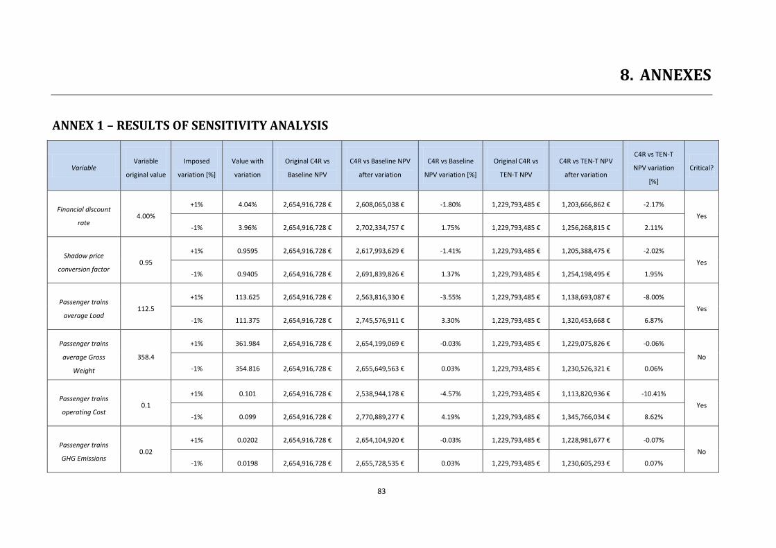
83
8. ANNEXES
ANNEX 1 – RESULTS OF SENSITIVITY ANALYSIS
Variable Variable
original value
Imposed
variation [%]
Value with
variation
Original C4R vs
Baseline NPV
C4R vs Baseline NPV
after variation
C4R vs Baseline
NPV variation [%]
Original C4R vs
TEN-T NPV
C4R vs TEN-T NPV
after variation
C4R vs TEN-T
NPV variation
[%]
Critical?
Financial discount
rate 4.00%
+1% 4.04% 2,654,916,728 € 2,608,065,038 € -1.80% 1,229,793,485 € 1,203,666,862 € -2.17%
Yes
-1% 3.96% 2,654,916,728 € 2,702,334,757 € 1.75% 1,229,793,485 € 1,256,268,815 € 2.11%
Shadow price
conversion factor 0.95
+1% 0.9595 2,654,916,728 € 2,617,993,629 € -1.41% 1,229,793,485 € 1,205,388,475 € -2.02%
Yes
-1% 0.9405 2,654,916,728 € 2,691,839,826 € 1.37% 1,229,793,485 € 1,254,198,495 € 1.95%
Passenger trains
average Load 112.5
+1% 113.625 2,654,916,728 € 2,563,816,330 € -3.55% 1,229,793,485 € 1,138,693,087 € -8.00%
Yes
-1% 111.375 2,654,916,728 € 2,745,576,911 € 3.30% 1,229,793,485 € 1,320,453,668 € 6.87%
Passenger trains
average Gross
Weight
358.4
+1% 361.984 2,654,916,728 € 2,654,199,069 € -0.03% 1,229,793,485 € 1,229,075,826 € -0.06%
No
-1% 354.816 2,654,916,728 € 2,655,649,563 € 0.03% 1,229,793,485 € 1,230,526,321 € 0.06%
Passenger trains
operating Cost 0.1
+1% 0.101 2,654,916,728 € 2,538,944,178 € -4.57% 1,229,793,485 € 1,113,820,936 € -10.41%
Yes
-1% 0.099 2,654,916,728 € 2,770,889,277 € 4.19% 1,229,793,485 € 1,345,766,034 € 8.62%
Passenger trains
GHG Emissions 0.02
+1% 0.0202 2,654,916,728 € 2,654,104,920 € -0.03% 1,229,793,485 € 1,228,981,677 € -0.07%
No
-1% 0.0198 2,654,916,728 € 2,655,728,535 € 0.03% 1,229,793,485 € 1,230,605,293 € 0.07%
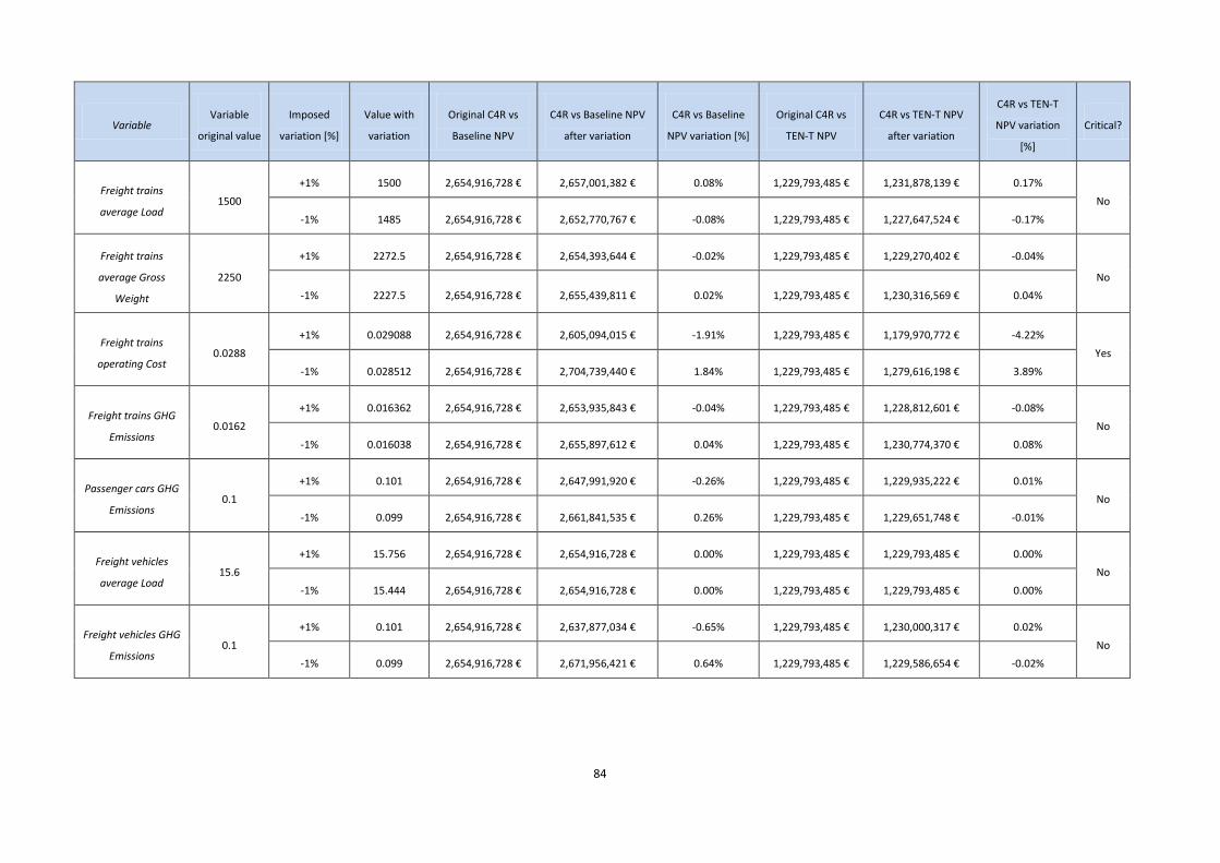
84
Variable Variable
original value
Imposed
variation [%]
Value with
variation
Original C4R vs
Baseline NPV
C4R vs Baseline NPV
after variation
C4R vs Baseline
NPV variation [%]
Original C4R vs
TEN-T NPV
C4R vs TEN-T NPV
after variation
C4R vs TEN-T
NPV variation
[%]
Critical?
Freight trains
average Load 1500
+1% 1500 2,654,916,728 € 2,657,001,382 € 0.08% 1,229,793,485 € 1,231,878,139 € 0.17%
No
-1% 1485 2,654,916,728 € 2,652,770,767 € -0.08% 1,229,793,485 € 1,227,647,524 € -0.17%
Freight trains
average Gross
Weight
2250
+1% 2272.5 2,654,916,728 € 2,654,393,644 € -0.02% 1,229,793,485 € 1,229,270,402 € -0.04%
No
-1% 2227.5 2,654,916,728 € 2,655,439,811 € 0.02% 1,229,793,485 € 1,230,316,569 € 0.04%
Freight trains
operating Cost 0.0288
+1% 0.029088 2,654,916,728 € 2,605,094,015 € -1.91% 1,229,793,485 € 1,179,970,772 € -4.22%
Yes
-1% 0.028512 2,654,916,728 € 2,704,739,440 € 1.84% 1,229,793,485 € 1,279,616,198 € 3.89%
Freight trains GHG
Emissions 0.0162
+1% 0.016362 2,654,916,728 € 2,653,935,843 € -0.04% 1,229,793,485 € 1,228,812,601 € -0.08%
No
-1% 0.016038 2,654,916,728 € 2,655,897,612 € 0.04% 1,229,793,485 € 1,230,774,370 € 0.08%
Passenger cars GHG
Emissions 0.1
+1% 0.101 2,654,916,728 € 2,647,991,920 € -0.26% 1,229,793,485 € 1,229,935,222 € 0.01%
No
-1% 0.099 2,654,916,728 € 2,661,841,535 € 0.26% 1,229,793,485 € 1,229,651,748 € -0.01%
Freight vehicles
average Load 15.6
+1% 15.756 2,654,916,728 € 2,654,916,728 € 0.00% 1,229,793,485 € 1,229,793,485 € 0.00%
No
-1% 15.444 2,654,916,728 € 2,654,916,728 € 0.00% 1,229,793,485 € 1,229,793,485 € 0.00%
Freight vehicles GHG
Emissions 0.1
+1% 0.101 2,654,916,728 € 2,637,877,034 € -0.65% 1,229,793,485 € 1,230,000,317 € 0.02%
No
-1% 0.099 2,654,916,728 € 2,671,956,421 € 0.64% 1,229,793,485 € 1,229,586,654 € -0.02%
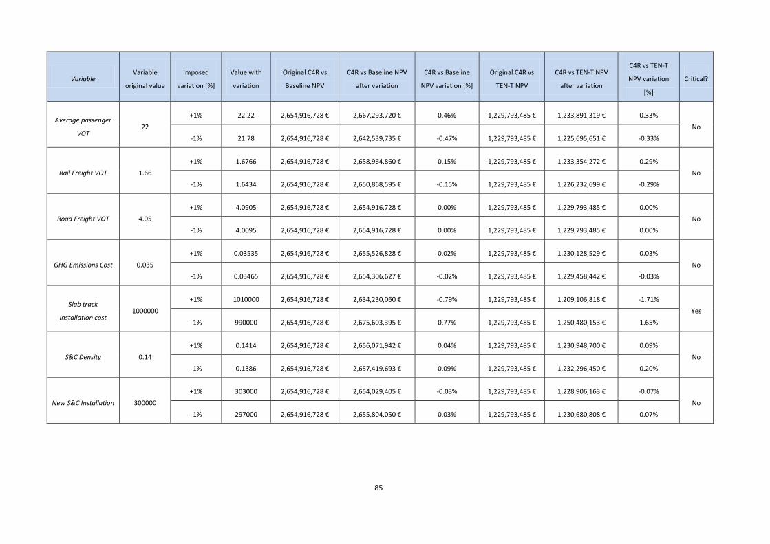
85
Variable Variable
original value
Imposed
variation [%]
Value with
variation
Original C4R vs
Baseline NPV
C4R vs Baseline NPV
after variation
C4R vs Baseline
NPV variation [%]
Original C4R vs
TEN-T NPV
C4R vs TEN-T NPV
after variation
C4R vs TEN-T
NPV variation
[%]
Critical?
Average passenger
VOT 22
+1% 22.22 2,654,916,728 € 2,667,293,720 € 0.46% 1,229,793,485 € 1,233,891,319 € 0.33%
No
-1% 21.78 2,654,916,728 € 2,642,539,735 € -0.47% 1,229,793,485 € 1,225,695,651 € -0.33%
Rail Freight VOT 1.66
+1% 1.6766 2,654,916,728 € 2,658,964,860 € 0.15% 1,229,793,485 € 1,233,354,272 € 0.29%
No
-1% 1.6434 2,654,916,728 € 2,650,868,595 € -0.15% 1,229,793,485 € 1,226,232,699 € -0.29%
Road Freight VOT 4.05
+1% 4.0905 2,654,916,728 € 2,654,916,728 € 0.00% 1,229,793,485 € 1,229,793,485 € 0.00%
No
-1% 4.0095 2,654,916,728 € 2,654,916,728 € 0.00% 1,229,793,485 € 1,229,793,485 € 0.00%
GHG Emissions Cost 0.035
+1% 0.03535 2,654,916,728 € 2,655,526,828 € 0.02% 1,229,793,485 € 1,230,128,529 € 0.03%
No
-1% 0.03465 2,654,916,728 € 2,654,306,627 € -0.02% 1,229,793,485 € 1,229,458,442 € -0.03%
Slab track
Installation cost 1000000
+1% 1010000 2,654,916,728 € 2,634,230,060 € -0.79% 1,229,793,485 € 1,209,106,818 € -1.71%
Yes
-1% 990000 2,654,916,728 € 2,675,603,395 € 0.77% 1,229,793,485 € 1,250,480,153 € 1.65%
S&C Density 0.14
+1% 0.1414 2,654,916,728 € 2,656,071,942 € 0.04% 1,229,793,485 € 1,230,948,700 € 0.09%
No
-1% 0.1386 2,654,916,728 € 2,657,419,693 € 0.09% 1,229,793,485 € 1,232,296,450 € 0.20%
New S&C Installation 300000
+1% 303000 2,654,916,728 € 2,654,029,405 € -0.03% 1,229,793,485 € 1,228,906,163 € -0.07%
No
-1% 297000 2,654,916,728 € 2,655,804,050 € 0.03% 1,229,793,485 € 1,230,680,808 € 0.07%
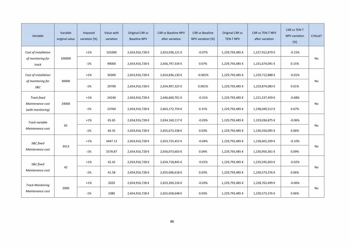
86
Variable Variable
original value
Imposed
variation [%]
Value with
variation
Original C4R vs
Baseline NPV
C4R vs Baseline NPV
after variation
C4R vs Baseline
NPV variation [%]
Original C4R vs
TEN-T NPV
C4R vs TEN-T NPV
after variation
C4R vs TEN-T
NPV variation
[%]
Critical?
Cost of installation
of monitoring for
track
100000
+1% 101000 2,654,916,728 € 2,653,036,121 € -0.07% 1,229,793,485 € 1,227,912,879 € -0.15%
No
-1% 99000 2,654,916,728 € 2,656,797,334 € 0.07% 1,229,793,485 € 1,231,674,091 € 0.15%
Cost of installation
of monitoring for
S&C
30000
+1% 30300 2,654,916,728 € 2,654,836,130 € -0.001% 1,229,793,485 € 1,229,712,888 € -0.01%
No
-1% 29700 2,654,916,728 € 2,654,997,325 € 0.001% 1,229,793,485 € 1,229,874,083 € 0.01%
Track fixed
Maintenance cost
(with monitoring)
24000
+1% 24240 2,654,916,728 € 2,646,660,701 € -0.31% 1,229,793,485 € 1,221,537,459 € -0.68%
No
-1% 23760 2,654,916,728 € 2,663,172,754 € 0.31% 1,229,793,485 € 1,238,049,512 € 0.67%
Track variable
Maintenance cost 65
+1% 65.65 2,654,916,728 € 2,654,160,117 € -0.03% 1,229,793,485 € 1,229,036,875 € -0.06%
No
-1% 64.35 2,654,916,728 € 2,655,673,338 € 0.03% 1,229,793,485 € 1,230,550,095 € 0.06%
S&C fixed
Maintenance cost 3413
+1% 3447.13 2,654,916,728 € 2,653,725,452 € -0.04% 1,229,793,485 € 1,228,602,209 € -0.10%
No
-1% 3378.87 2,654,916,728 € 2,656,073,603 € 0.04% 1,229,793,485 € 1,230,950,361 € 0.09%
S&C fixed
Maintenance cost 42
+1% 42.42 2,654,916,728 € 2,654,718,845 € -0.01% 1,229,793,485 € 1,229,595,603 € -0.02%
No
-1% 41.58 2,654,916,728 € 2,655,696,618 € 0.03% 1,229,793,485 € 1,230,573,376 € 0.06%
Track Monitoring
Maintenance cost 2000
+1% 2020 2,654,916,728 € 2,653,269,226 € -0.03% 1,229,793,485 € 1,228,763,499 € -0.06%
No
-1% 1080 2,654,916,728 € 2,655,658,648 € 0.03% 1,229,793,485 € 1,230,573,376 € 0.06%
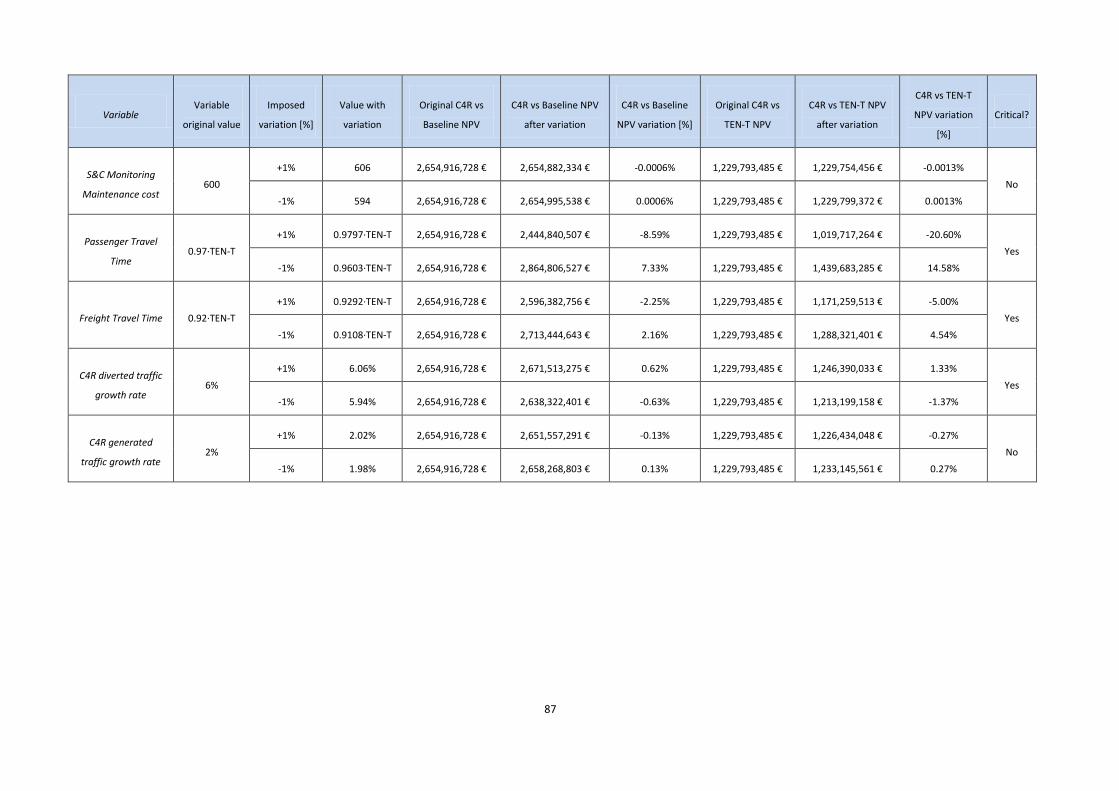
87
Variable Variable
original value
Imposed
variation [%]
Value with
variation
Original C4R vs
Baseline NPV
C4R vs Baseline NPV
after variation
C4R vs Baseline
NPV variation [%]
Original C4R vs
TEN-T NPV
C4R vs TEN-T NPV
after variation
C4R vs TEN-T
NPV variation
[%]
Critical?
S&C Monitoring
Maintenance cost 600
+1% 606 2,654,916,728 € 2,654,882,334 € -0.0006% 1,229,793,485 € 1,229,754,456 € -0.0013%
No
-1% 594 2,654,916,728 € 2,654,995,538 € 0.0006% 1,229,793,485 € 1,229,799,372 € 0.0013%
Passenger Travel
Time 0.97·TEN-T
+1% 0.9797·TEN-T 2,654,916,728 € 2,444,840,507 € -8.59% 1,229,793,485 € 1,019,717,264 € -20.60%
Yes
-1% 0.9603·TEN-T 2,654,916,728 € 2,864,806,527 € 7.33% 1,229,793,485 € 1,439,683,285 € 14.58%
Freight Travel Time 0.92·TEN-T
+1% 0.9292·TEN-T 2,654,916,728 € 2,596,382,756 € -2.25% 1,229,793,485 € 1,171,259,513 € -5.00%
Yes
-1% 0.9108·TEN-T 2,654,916,728 € 2,713,444,643 € 2.16% 1,229,793,485 € 1,288,321,401 € 4.54%
C4R diverted traffic
growth rate 6%
+1% 6.06% 2,654,916,728 € 2,671,513,275 € 0.62% 1,229,793,485 € 1,246,390,033 € 1.33%
Yes
-1% 5.94% 2,654,916,728 € 2,638,322,401 € -0.63% 1,229,793,485 € 1,213,199,158 € -1.37%
C4R generated
traffic growth rate 2%
+1% 2.02% 2,654,916,728 € 2,651,557,291 € -0.13% 1,229,793,485 € 1,226,434,048 € -0.27%
No
-1% 1.98% 2,654,916,728 € 2,658,268,803 € 0.13% 1,229,793,485 € 1,233,145,561 € 0.27%
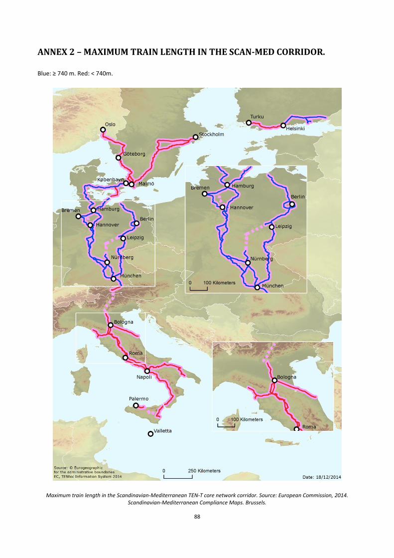
88
ANNEX 2 – MAXIMUM TRAIN LENGTH IN THE SCAN-MED CORRIDOR.
Blue: ≥ 740 m. Red: < 740m.
Maximum train length in the Scandinavian-Mediterranean TEN-T core network corridor. Source: European Commission, 2014. Scandinavian-Mediterranean Compliance Maps. Brussels.