Modelling the impact of policy interventions on income in ...

Modelling the impact of policy interventions on income in Scotland

Richard Marsh, Anouk Berthier and Thomas Kane, 4-consultingDecember 2017

Published by NHS Health Scotland

1 South Gyle CrescentEdinburgh EH12 9EB

© NHS Health Scotland 2017

All rights reserved. Material contained in this publication may not be reproduced in whole or part without prior permission of NHS Health Scotland (or other copyright owners).While every effort is made to ensure that the information given here is accurate, no legal responsibility is accepted for any errors, omissions or misleading statements.

NHS Health Scotland is a WHO Collaborating Centre for Health Promotion and Public Health Development.

This resource may also be made available on request in the following formats:

0131 314 5300

[email protected]

mailto:nhs.healthscotland-alternativeformats%40nhs.net?subject=

i

Contents

Acknowledgements ............................................................................................ 1 Abbreviations ...................................................................................................... 1 Executive summary ............................................................................................ 2 1. Introduction ............................................................................................... 5 1.1 Background ................................................................................................. 5 1.2 Aim .............................................................................................................. 5 1.3 Report structure .......................................................................................... 6 2. Methods ..................................................................................................... 6 2.1 Background ................................................................................................. 6 2.2 EUROMOD ................................................................................................. 7 2.3 Family Resources Survey ........................................................................... 8 2.4 Policy scenarios modelled ........................................................................... 9 2.5 Simulation of taxes and benefits in EUROMOD ........................................ 10 2.6 Benefit take-up rates ................................................................................. 11 2.7 Integrating behavioural responses into EUROMOD .................................. 11 2.8 Multiplier effects ........................................................................................ 12 3. Results ..................................................................................................... 123.1 Overview ................................................................................................... 12 3.2 Basic rate of income tax decreased by 1p ................................................ 14 3.2.1 Policy scenario ....................................................................................... 14 3.2.2 Impact on poverty and income inequality ............................................... 14 3.2.3 Impact on household disposable income ............................................... 14 3.3 Decreasing income tax .............................................................................. 16 3.3.1 Policy scenario ....................................................................................... 16 3.3.2 Impact on poverty and income inequality ............................................... 16 3.3.3 Impact on household disposable income ............................................... 17 3.4 Decreasing the Personal Allowance .......................................................... 18 3.4.1 Policy scenario ....................................................................................... 18 3.4.2 Impact on poverty and income inequality ............................................... 18 3.4.3 Impact on household disposable income ............................................... 19 3.5 Increasing the Carer’s Allowance .............................................................. 20 3.5.1 Policy scenario ....................................................................................... 20 3.5.2 Impact on poverty and income inequality ............................................... 20 3.5.3 Impact on household disposable income ............................................... 21 3.6 Introducing a Citizen’s Income .................................................................. 22 3.6.1 Policy scenario ....................................................................................... 22 3.6.2 Impact on poverty and income inequality ............................................... 23 3.6.3 Impact on household disposable income ............................................... 24 3.7 Increasing Council Tax for bands E-H ....................................................... 25 3.7.1 Policy scenario ....................................................................................... 25 3.7.2 Impact on poverty and income inequality ............................................... 25 3.7.3 Impact on household disposable income ............................................... 25 3.8 Replacing Council Tax with a Local income tax ........................................ 27 3.8.1 Policy scenario ....................................................................................... 27

ii

3.8.2 Impact on poverty and income inequality ............................................... 27 3.8.3 Impact on household disposable income ............................................... 28 3.9 Impact on taxes paid and benefits received .............................................. 29 3.10 Multiplier effects ........................................................................................ 30 3.11 Summary of findings .............................................................................. 31 4. Discussion ............................................................................................... 324.1 Main results ............................................................................................... 32 4.2 Limitations ................................................................................................. 34 4.2.1 Limitations of EUROMOD and FRS ....................................................... 34 4.2.2 Policy scenarios ..................................................................................... 35 4.3 Recommendations .................................................................................... 36 5. References ............................................................................................... 37

Appendix 1: Taxes, benefits and modelling in EUROMOD ................................. 42 Appendix 2: Benefit and tax credit take-up rates in EUROMOD ......................... 47 Appendix 3: A review of behavioural responses to tax and benefit changes ...... 48 Appendix 4: Empirical evidence on TIEs ............................................................. 57 Appendix 5: Case study, 50p additional rate 2010-11 to 2013-14 ...................... 64 Appendix 6: Estimating multiplier effects ............................................................ 67 Appendix 7: Bridging results between income and deprivation ........................... 69

1

Acknowledgements We are grateful to Ralph Leishman (4-consulting) and Dr Paola De Agostini, (University of Essex) Abbreviations AHC After Housing Costs BHC Before Housing Costs DDA Disability Discrimination Act DWP Department for Work and Pensions EFO Economic and Fiscal Outlook EMTR Effective Marginal Tax Rate ESA Employment and Support Allowance FDI Foreign Direct Investment FRS Family Resources Survey HDI Household Disposable Income HMRC HM Revenue and Customs IFS Institute for Fiscal Studies III Informing Investment to reduce Inequalities IRS Internal Revenue Service ISER Institute for Social and Economic Research JSA Jobseeker’s Allowance NatCen National Centre for Social Research OBR Office for Budget Responsibility OECD Organisation for Economic Co-Operation and Development ONS Office for National Statistics PAF Postcode Address File PTR Participation Tax Rate RR Replacement Rate SDA Severe Disability Allowance SRIT Scottish Rate of Income Tax TIE Taxable Income Elasticity VAT Value Added Tax

2

Executive summary

Background Health inequalities in Scotland are worse than elsewhere in Central and Western Europe and have therefore become a particular focus for public policy. NHS Health Scotland is the lead organisation providing, collating and interpreting evidence, with the aim of supporting policy and practice development to reduce health inequalities and improve health in Scotland.

There is therefore a need to be able to model the potential effects of new policies for each of these aims separately, but it is essential to know the simultaneous effects on both aims together, in order to make balanced policy decisions.

Aim The overall aim of this research was to estimate the impact on household income distribution in Scotland of a broad range of policies. This would allow modelling of policy effects on health inequalities and health improvement through the Scottish Public Health Observatory’s Informing Investment to reduce health Inequalities (‘III’) tool.

Methods The EUROMOD model was used to estimate the impact of a range of policy scenarios on household incomes. EUROMOD is a detailed model of the UK tax and benefit system that calculates liabilities to income tax, National Insurance contributions and council tax, as well as entitlements to the main benefits and tax credits. It is part of a European-wide project and is managed in the UK by a team based in the Institute for Social and Economic Research (ISER) at the University of Essex. EUROMOD enables users to model changes to the tax and benefit system. The effects of those changes can be seen across a range of variables including household income, tax revenues, public expenditure and inequality.

The policy scenarios considered for Scotland were as follows: • The basic rate of income tax was reduced by 1p.• The basic rate of income tax was increased by 5p.• The higher rate of income tax was increased by 5p.• The basic, higher and additional rates of income tax were reduced by 1p.• Personal allowance was reduced by £1,000.• Personal allowance was increased by £1,000.• Carer’s allowance was increased by £10 a week.• A citizen's income (basic income) was introduced.• Council tax was increased among higher bands.• Council tax was replaced with a local income tax• A wealth tax was introduced based on high value properties.

3

Summary of key results The Summary Table provides a summary of the impact of the policy scenarios modelled on average equivalised household disposable income. The results presented do not incorporate the impact of behavioural responses to the modelled policy scenarios. They also do not account for secondary impacts such as impacts on public spending or the redistribution/use of additional tax revenue. Introducing a citizen’s income was modelled to have the largest impact on household disposable income; however, the scenario should be considered as illustrative as it did not incorporate other changes to the tax and benefit system. Replacing council tax with a local income tax was also modelled to increase household disposable incomes in Scotland. These policies were also estimated to result in the largest reduction in income inequalities in Scotland by disproportionately raising the income of those on lower incomes. Increasing the carer’s allowance payments did not make much of an impact on poverty rates or inequality, but the additional income is well targeted at the lowest income households. Changes in the rate of income tax are useful in demonstrating the relative impact of the basic, higher and additional rates of income tax. Raising the basic rate of income tax by 1p has a higher impact on higher income households in Scotland than raising the higher or additional rate of income tax by 1p. This is because the number of households paying income tax at the higher or additional rates is relatively small. The results show that efforts to increase household disposable income among Scotland’s low income households may also increase income among higher income households. Introducing a citizen’s income and replacing council tax with a local income tax were the most expensive policy scenarios. They might therefore be best considered in combination with the impacts of tax raising policies.

4

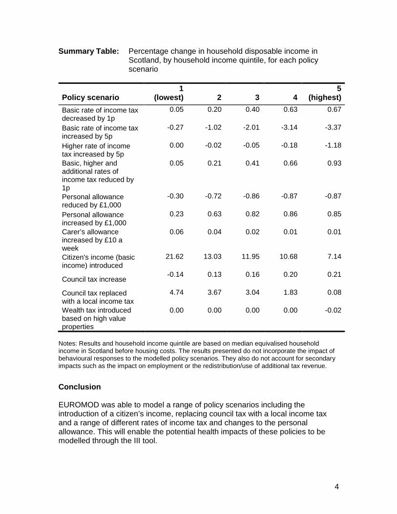
Summary Table: Percentage change in household disposable income in Scotland, by household income quintile, for each policy scenario

Policy scenario 1

(lowest) 2 3 4 5

(highest) Basic rate of income tax decreased by 1p

0.05 0.20 0.40 0.63 0.67

Basic rate of income tax increased by 5p

-0.27 -1.02 -2.01 -3.14 -3.37

Higher rate of income tax increased by 5p

0.00 -0.02 -0.05 -0.18 -1.18

Basic, higher and additional rates of income tax reduced by 1p

0.05 0.21 0.41 0.66 0.93

Personal allowance reduced by £1,000

-0.30 -0.72 -0.86 -0.87 -0.87

Personal allowance increased by £1,000

0.23 0.63 0.82 0.86 0.85

Carer’s allowance increased by £10 a week

0.06 0.04 0.02 0.01 0.01

Citizen's income (basic income) introduced

21.62 13.03 11.95 10.68 7.14

Council tax increase -0.14 0.13 0.16 0.20 0.21

Council tax replaced with a local income tax

4.74 3.67 3.04 1.83 0.08

Wealth tax introduced based on high value properties

0.00 0.00 0.00 0.00 -0.02

Notes: Results and household income quintile are based on median equivalised household income in Scotland before housing costs. The results presented do not incorporate the impact of behavioural responses to the modelled policy scenarios. They also do not account for secondary impacts such as the impact on employment or the redistribution/use of additional tax revenue. Conclusion EUROMOD was able to model a range of policy scenarios including the introduction of a citizen’s income, replacing council tax with a local income tax and a range of different rates of income tax and changes to the personal allowance. This will enable the potential health impacts of these policies to be modelled through the III tool.

5

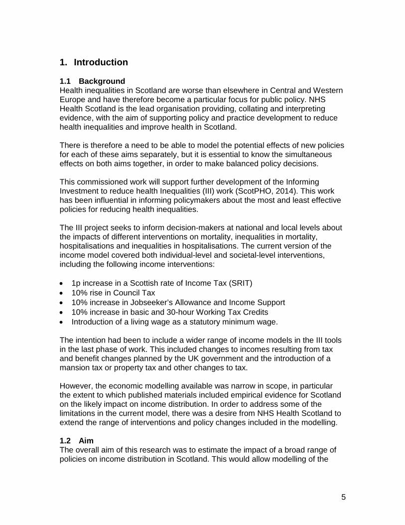
1. Introduction 1.1 Background Health inequalities in Scotland are worse than elsewhere in Central and Western Europe and have therefore become a particular focus for public policy. NHS Health Scotland is the lead organisation providing, collating and interpreting evidence, with the aim of supporting policy and practice development to reduce health inequalities and improve health in Scotland. There is therefore a need to be able to model the potential effects of new policies for each of these aims separately, but it is essential to know the simultaneous effects on both aims together, in order to make balanced policy decisions. This commissioned work will support further development of the Informing Investment to reduce health Inequalities (III) work (ScotPHO, 2014). This work has been influential in informing policymakers about the most and least effective policies for reducing health inequalities. The III project seeks to inform decision-makers at national and local levels about the impacts of different interventions on mortality, inequalities in mortality, hospitalisations and inequalities in hospitalisations. The current version of the income model covered both individual-level and societal-level interventions, including the following income interventions: • 1p increase in a Scottish rate of Income Tax (SRIT) • 10% rise in Council Tax • 10% increase in Jobseeker’s Allowance and Income Support • 10% increase in basic and 30-hour Working Tax Credits • Introduction of a living wage as a statutory minimum wage. The intention had been to include a wider range of income models in the III tools in the last phase of work. This included changes to incomes resulting from tax and benefit changes planned by the UK government and the introduction of a mansion tax or property tax and other changes to tax. However, the economic modelling available was narrow in scope, in particular the extent to which published materials included empirical evidence for Scotland on the likely impact on income distribution. In order to address some of the limitations in the current model, there was a desire from NHS Health Scotland to extend the range of interventions and policy changes included in the modelling. 1.2 Aim The overall aim of this research was to estimate the impact of a broad range of policies on income distribution in Scotland. This would allow modelling of the

6

impact on health inequalities through the Informing Investment to reduce health Inequalities (III) tool. 1.3 Report structure The remainder of this report sets out the methods used to model the policy impacts, the data sources used to populate the models, and how impacts were analysed. The report also provides an overview and interpretation of the modelled policy scenarios. To manage the large amount of data produced during this project, additional results have been provided electronically in a Microsoft Excel workbook. 2. Methods 2.1 Background A wide range of policy scenarios were discussed at the start of the research project. The Scottish Public Health Observatory (ScotPHO) website describes the policy scenarios to which the III tools have previously been applied (ScotPHO, 2014). The tax-benefit model developed during this research project would therefore need to be reasonably comprehensive. Following the inclusion of the previous tax-benefit model to inform the III tool, there was a desire to develop a more interactive tax-benefit model (as outlined in the previous section). Additionally, the tax-benefit system has changed since the previous research. For example, the UK-wide National Living Wage, payable to workers aged over 25 years, came into effect on 1 April 2016. In addition to providing modelled outcomes, this research project sought to provide an opportunity for users to access the tax-benefit model. This would allow further changes to taxes and benefits to be modelled with outcomes updated accordingly. A microsimulation model is already available and is currently used to inform policies on taxes, welfare and inequality in Scotland. The EUROMOD model has been used by the Scottish Parliament, and academics to model the impact of changes to taxes and benefits on income distribution and inequality. The key strengths of the EUROMOD model include: • highly flexible policy settings • intuitive user interface • special-purpose tax-benefit modelling language • extensive library of policies • continual updates and development • accessible and transparent modelling process.

7

EUROMOD can be linked to, or used alongside, other types of model (behavioural, macro-economic or environmental) as a tax-benefit policy calculator or to provide a distributional perspective. EUROMOD’s flexibility means that it can be adapted to shortcut the process of building tax-benefit models with potentially comparable outputs for any country. 2.2 EUROMOD EUROMOD is a detailed model of the UK tax and benefit system that calculates liabilities to income tax, National Insurance contributions and council tax, as well as entitlements to the main benefits and tax credits. It is part of a European-wide project and is managed in the UK by a team based in the Institute for Social and Economic Research (ISER) at the University of Essex. EUROMOD enables users to model changes to the tax and benefit system and to see the effect that this has on a range of variables (e.g. household income, tax revenues, public expenditure, inequality, etc.).i EUROMOD uses two input files and produces one output file per modelling run. The input files are: • The Family Resources Survey (FRS) (see Section 2.2.4). • A file containing tax requirements and benefit and tax credit entitlements that

apply in June in a given year. The effect of a policy change can be analysed by comparing the input dataset and the output file. This is a straightforward exercise as the output file is in the same format as the input dataset. There are different simulated values for each survey respondent and each variable based on the system that is being modelled. The effect of a given policy can therefore be assessed across a range of variables that cover the impact on the population on the one hand (for instance, disposable income, benefits received, taxes paid) and the impact on public finances on the other (tax revenues, social security expenditure). The major benefits of EUROMOD are its user-friendly interface, the high level of flexibility the policy settings have, that ISER keep the tax and benefit rules up-to-date (the model is generally updated within 3 months of a UK Budget, Statement or Spending Review), and the existence of some sub-regional data. For instance, the Council Tax freeze up to 2016 in Scotland was incorporated into the modelling. The results, for instance the effect of disposable income, are generally calculated for individuals or households according to household disposable income (HDI) i The EUROMOD Country Report for the UK (2011-2015) can be accessed here: https://www.euromod.ac.uk/sites/default/files/country-reports/year6/Y6_CR_UK_final_13-04-2016.pdf

https://www.euromod.ac.uk/sites/default/files/country-reports/year6/Y6_CR_UK_final_13-04-2016.pdf

https://www.euromod.ac.uk/sites/default/files/country-reports/year6/Y6_CR_UK_final_13-04-2016.pdf

8

equivalised by the “modified OECD” equivalence scale. HDI are calculated as the sum of all income sources of all household members net of income tax and social insurance contributions.ii 2.3 Family Resources Survey The FRS is an annual population survey carried out by the Office for National Statistics (ONS), which collects a wide range of information on the income and circumstances of private households in the UK. The FRS sample is designed to be representative of private households in the United Kingdom.iii The Great Britain FRS sample is drawn from the Royal Mail’s small users Postcode Address File (PAF). In each eligible household, the aim is to interview all adults aged 16 years and over, except those aged 16 to 19 years who were classed as dependent children (UK Government 2015). The most recent version available for use in EUROMOD is 2013-14: this includes 46,166 individuals in 20,137 households in the UK as a whole, and 6,378 individuals in 3,000 households in Scotland. Once weighted, this represents 5,227,999 individuals in 2,406,370 households in Scotland. As EUROMOD currently uses the 2013-14 FRS, when modelling policy changes after 2013, the monetary variables that relate to income are projected forwards using the Office for Budget Responsibility’s Economic and Fiscal Outlook (EFO) (this is a bi-annual publication). Caution must be used when interpreting results as projecting data from 2013 to 2016 in this manner may not capture the full effect of the recession. Indeed, changes in the composition or distribution of market incomes (e.g. inequality) since 2013 are not modelled, except those captured by updating income source. In addition, and perhaps most importantly in the context of modelling in Scotland relative to the UK as a whole, the FRS 2013/14 is not adjusted to reflect demographic changes. Thus, the modelling, as it uses the FRS 2013/14, is based on a weighted population of 5,227,999 individuals. This is 2.7% lower than the estimated population of Scotland as at 30 June 2015, which stood at 5,373,000 (ONS 2016). Using data provided in the EFO, it is possible to model forwards using EUROMOD up to 2020-21. However, this is subject to huge uncertainty given the effect that unexpected changes to the economic situation and as-yet unannounced policy changes between now and then would have.

ii The weights in the OECD equivalence are: first adult=1; additional people aged 14+ = 0.5;

additional people aged under 14 = 0.3. iii Therefore, it does not include institutionalised populations.

https://www.ons.gov.uk/peoplepopulationandcommunity/populationandmigration/populationestimates/bulletins/annualmidyearpopulationestimates/latest

9

Analysis was undertaken using the standard EUROMOD model but with three additional areas of work. First, the standard model was extended to include characteristics of interest to NHS Health Scotland (including age, gender, disability, ethnicity and marital status). The analysis of income changes by gender analysis was undertaken at the individual (not equivalised) level rather than household level. This was because the majority of households in Scotland contained both males and females and changes to household income do not provide meaningful information for outcomes by gender. Second, the modelled outcomes were adjusted for behavioural responses. Finally, the outcomes were adjusted to take into account direct and multiplier effects. The approaches used to estimate behavioural responses and multiplier effects are outlined in sections 2.4 and 2.5, respectively. 2.4 Policy scenarios modelled The policy scenarios considered for Scotland were as follows: • The basic rate of income tax was reduced by 1p. • The basic rate of income tax was increased by 5p. • The higher rate of income tax was increased by 5p. • The basic, higher and additional rates of income tax were reduced by 1p. • Personal allowance was reduced by £1,000. • Personal allowance was increased by £1,000. • Carer’s allowance was increased by £10 a week. • A citizen's income (basic income) was introduced. • Council tax was increased among higher bands.iv • Council tax was replaced with a local income tax • A wealth tax was introduced based on high value properties. Modelled outcomes for all of the above policy scenarios were also produced for the UK based on the same modelled assumptions. The only exception was the introduction of a wealth tax based on high value properties which was not modelled for the UK. All of the scenarios listed in this section are available in the accompanying Microsoft Excel workbook. The standard EUROMOD model was extended to include estimates by protected characteristics of interest to NHS Health Scotland (including age, gender, disability, ethnicity and marital status). The standard EUROMOD model produces outcomes based on equivalised household income before housing costs. An estimate of housing costs from the FRS was added to the EUROMOD model to also produce estimates of changes in equivalised household income after housing costs. The modelled outcomes included poverty rates and measures of inequality. Households at risk of being in poverty were those with equivalised disposable

iv Note that a version of this policy was introduced by the Scottish Government in 2017 (see http://www.gov.scot/Topics/Government/local-government/17999/counciltax )

10

household income (before housing costs) below 60% of the median equivalised disposable household income. The assumed benefit and tax credit take-up rates in EUROMOD used in the scenarios are shown in Appendix 2. Changes in the poverty rates arise through income changes among each of the above cohorts and changes to median income for the whole population. Poverty rates were measured for: • Children: those aged 18 years or younger. • Working age people: those aged between 19 and 64 years (inclusive). • Working age people (economically active): working age people with

employment or self-employment income. • Elderly people: those aged 65 years or older. The outcomes from the standard EUROMOD model include the Gini coefficient (based on equivalised household income before housing costs). The Gini coefficient is a widely-used measure of income inequality. It is expressed as a number between 0 and 1. A Gini coefficient of 0 represents perfect income equality, where everyone has the same income. A Gini coefficient of 1 represents perfect income inequality, with all income accruing to one specific group or person. 2.5 Simulation of taxes and benefits in EUROMOD EUROMOD enables the user to model the effect of a policy, this is called “simulating” the policy. Policies are modelled to varying degrees of accuracy and some policies cannot be simulated at all. If the eligibility (for benefits) and liability criteria (for taxes) are present in the FRS, then the policy is fully simulated in EUROMOD. If the data are not available, the policy can only be partially simulated or not at all, in which case if another variable in the FRS provides the value of the tax or benefit, some simple modifications can be made to the tax or benefit in question. For instance, the FRS does not contain sufficient data on carers (namely on the benefits received by the person being cared for, carer working hours, etc.) for EUROMOD to be able to fully simulate Carer’s Allowance. However, the FRS does ask whether the respondent is in receipt of Carer’s Allowance. Carer’s Allowance is “imputed” from the survey data in EUROMOD. Therefore, EUROMOD can model an absolute or relative change in Carer’s Allowance but cannot change the eligibility criteria for this benefit. Appendix 1 summarises the main taxes and social security benefits in the UK and explains whether they are simulated in EUROMOD. It also includes information on how well they are simulated in EUROMOD compared to most recent available administrative datasets from official sources such as the Department for Work and Pensions (DWP).

11

EUROMOD uses a slightly modified version of the FRS in order to make it compatible with a micro-simulation model and try and ameliorate known margins of error over the years. This is discussed in the University of Essex’s report on EUROMOD in the UK (Agostini & Sutherland, 2016). It is important to note that under-representation of non-simulated benefits has implications for the values of the simulated benefits, if these depend in some way upon receipt of the non-simulated benefits. Where receipt of the latter automatically “passports” eligibility for a simulated benefit, this will lead to under-estimation of that benefit. On the other hand, if income from the non-simulated benefit is included in a means-test for a simulated benefit, under-estimation of the former will lead to over-estimation of the latter. Similar mechanisms apply in reverse to the case of over-estimation of non-simulated benefits. 2.6 Benefit take-up rates EUROMOD measures eligibility for benefits. If all those eligible were considered to be in receipt of those benefits, the model would overestimate the number of people on benefits as not all those who are eligible actually claim them. EUROMOD adjusts for this by using a “take-up correction” based on DWP and HM Revenue and Customs (HMRC) data. For example, EUROMOD assumes that 6% of lone parents do not receive the Child Tax Credit and Working Tax Credit they are entitled to. Appendix 2 shows the take-up rates for the benefits that are simulated in EUROMOD. Setting take-up rates based on best available data allows for much more accurate modelling. However, EUROMOD is still limited by a number of factors that must be taken into account in order to produce high quality modelling that is explicit on the error margins involved. 2.7 Integrating behavioural responses into EUROMOD EUROMOD is a static model: it calculates only the “mechanical” effect of a policy change. A literature review was undertaken to assess the evidence on behavioural responses to changes in taxes and benefits, including changes in tax planning, migration and labour supply responses. The review is presented in Appendix 3. No account is made for behavioural responses in the results presented in this report with the exception of the progressive change in female pension age, for which EUROMOD includes a minor behavioural response (Agostini & Sutherland 2016).

12

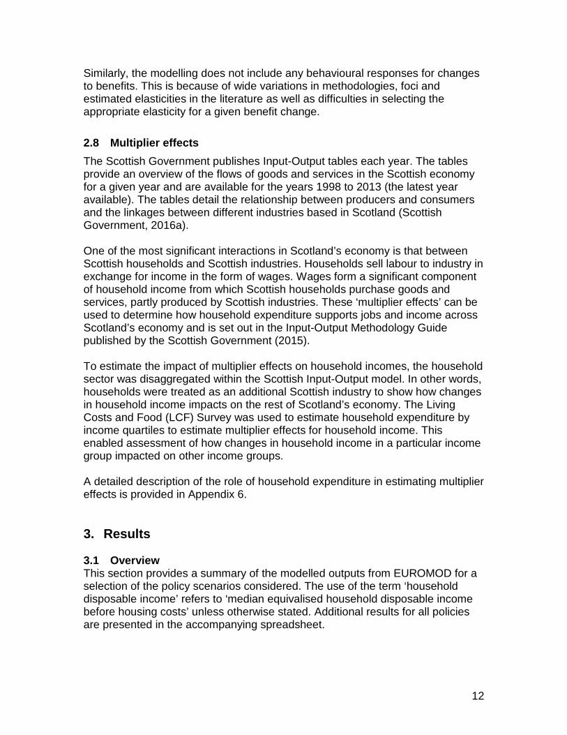
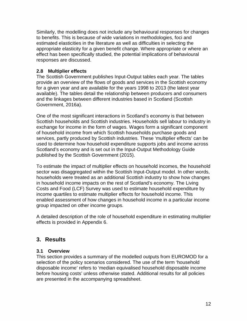
Similarly, the modelling does not include any behavioural responses for changes to benefits. This is because of wide variations in methodologies, foci and estimated elasticities in the literature as well as difficulties in selecting the appropriate elasticity for a given benefit change. 2.8 Multiplier effects The Scottish Government publishes Input-Output tables each year. The tables provide an overview of the flows of goods and services in the Scottish economy for a given year and are available for the years 1998 to 2013 (the latest year available). The tables detail the relationship between producers and consumers and the linkages between different industries based in Scotland (Scottish Government, 2016a). One of the most significant interactions in Scotland’s economy is that between Scottish households and Scottish industries. Households sell labour to industry in exchange for income in the form of wages. Wages form a significant component of household income from which Scottish households purchase goods and services, partly produced by Scottish industries. These ‘multiplier effects’ can be used to determine how household expenditure supports jobs and income across Scotland’s economy and is set out in the Input-Output Methodology Guide published by the Scottish Government (2015). To estimate the impact of multiplier effects on household incomes, the household sector was disaggregated within the Scottish Input-Output model. In other words, households were treated as an additional Scottish industry to show how changes in household income impacts on the rest of Scotland’s economy. The Living Costs and Food (LCF) Survey was used to estimate household expenditure by income quartiles to estimate multiplier effects for household income. This enabled assessment of how changes in household income in a particular income group impacted on other income groups. A detailed description of the role of household expenditure in estimating multiplier effects is provided in Appendix 6. 3. Results 3.1 Overview This section provides a summary of the modelled outputs from EUROMOD for a selection of the policy scenarios considered. The use of the term ‘household disposable income’ refers to ‘median equivalised household disposable income before housing costs’ unless otherwise stated. Additional results for all policies are presented in the accompanying spreadsheet.

12

Similarly, the modelling does not include any behavioural responses for changes to benefits. This is because of wide variations in methodologies, foci and estimated elasticities in the literature as well as difficulties in selecting the appropriate elasticity for a given benefit change. Where appropriate or where an effect has been specifically studied, the potential implications of behavioural responses are discussed. 2.8 Multiplier effects The Scottish Government publishes Input-Output tables each year. The tables provide an overview of the flows of goods and services in the Scottish economy for a given year and are available for the years 1998 to 2013 (the latest year available). The tables detail the relationship between producers and consumers and the linkages between different industries based in Scotland (Scottish Government, 2016a). One of the most significant interactions in Scotland’s economy is that between Scottish households and Scottish industries. Households sell labour to industry in exchange for income in the form of wages. Wages form a significant component of household income from which Scottish households purchase goods and services, partly produced by Scottish industries. These ‘multiplier effects’ can be used to determine how household expenditure supports jobs and income across Scotland’s economy and is set out in the Input-Output Methodology Guide published by the Scottish Government (2015). To estimate the impact of multiplier effects on household incomes, the household sector was disaggregated within the Scottish Input-Output model. In other words, households were treated as an additional Scottish industry to show how changes in household income impacts on the rest of Scotland’s economy. The Living Costs and Food (LCF) Survey was used to estimate household expenditure by income quartiles to estimate multiplier effects for household income. This enabled assessment of how changes in household income in a particular income group impacted on other income groups. A detailed description of the role of household expenditure in estimating multiplier effects is provided in Appendix 6. 3. Results 3.1 Overview This section provides a summary of the modelled outputs from EUROMOD for a selection of the policy scenarios considered. The use of the term ‘household disposable income’ refers to ‘median equivalised household disposable income before housing costs’ unless otherwise stated. Additional results for all policies are presented in the accompanying spreadsheet.

13

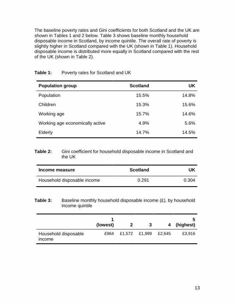
The baseline poverty rates and Gini coefficients for both Scotland and the UK are shown in Tables 1 and 2 below. Table 3 shows baseline monthly household disposable income in Scotland, by income quintile. The overall rate of poverty is slightly higher in Scotland compared with the UK (shown in Table 1). Household disposable income is distributed more equally in Scotland compared with the rest of the UK (shown in Table 2). Table 1: Poverty rates for Scotland and UK

Population group Scotland UK

Population 15.5% 14.8%

Children 15.3% 15.6%

Working age 15.7% 14.6%

Working age economically active 4.9% 5.6%

Elderly 14.7% 14.5%

Table 2: Gini coefficient for household disposable income in Scotland and

the UK

Income measure Scotland UK

Household disposable income 0.291 0.304

Table 3: Baseline monthly household disposable income (£), by household

income quintile

1 (lowest) 2 3 4

5 (highest)

Household disposable income

£964 £1,572 £1,999 £2,645 £3,916

14

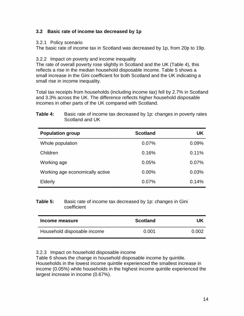
3.2 Basic rate of income tax decreased by 1p 3.2.1 Policy scenario The basic rate of income tax in Scotland was decreased by 1p, from 20p to 19p. 3.2.2 Impact on poverty and income inequality The rate of overall poverty rose slightly in Scotland and the UK (Table 4), this reflects a rise in the median household disposable income. Table 5 shows a small increase in the Gini coefficient for both Scotland and the UK indicating a small rise in income inequality. Total tax receipts from households (including income tax) fell by 2.7% in Scotland and 3.3% across the UK. The difference reflects higher household disposable incomes in other parts of the UK compared with Scotland. Table 4: Basic rate of income tax decreased by 1p: changes in poverty rates

Scotland and UK


Whole population 0.07% 0.09%




Elderly 0.07% 0.14%

Table 5: Basic rate of income tax decreased by 1p: changes in Gini

coefficient


Household disposable income 0.001 0.002

3.2.3 Impact on household disposable income Table 6 shows the change in household disposable income by quintile. Households in the lowest income quintile experienced the smallest increase in income (0.05%) while households in the highest income quintile experienced the largest increase in income (0.67%).

15

Table 6: Basic rate of income tax decreased by 1p: change in household

disposable income, by household income quintile

1 (lowest) 2 3 4

5 (highest)

Change in household disposable income (%)

0.05 0.20 0.40 0.63 0.67

Table 7 shows the increase in household income was higher among households without any disabled individuals. This included all individuals using the Disability Discrimination Act core definition. There was little difference in the change in household income when the ethnic group of the household reference person was considered. Table 7: Basic rate of income tax decreased by 1p: change in household

disposable income, by protected characteristics

Protected characteristic Change in household disposable income (%)

Disability

All households with disabled individuals 0.33

Households with no disabled individuals 0.57

Ethnicity

Household reference person belongs to ethnic minority group 0.45

Other households 0.50

Gender

Male 0.58

Female 0.41

Marital status

Married or in civil partnership 0.56

Not married or in civil partnership 0.45

16

The increase in income was slightly higher among males than among females. This is likely to reflect higher incomes, and therefore income tax paid, among males in Scotland. Table 7 also shows that the increase in income was marginally higher among households where the household reference person was married or in a civil partnership. The five-year age group in Scotland which saw the largest increase in disposable income (before housing costs) was 30-34 year olds (0.62%). Those aged 16-19 years old in Scotland saw the lowest increase in disposable income (close to zero percent). 3.3 Decreasing income tax 3.3.1 Policy scenario Income tax was decreased by 1p on earnings at the basic, higher and additional rates (19p, 39p, and 44p). 3.3.2 Impact on poverty and income inequality Table 8 shows the change in poverty rates resulting from decreasing all income tax rates. The decrease across all rates of income tax resulted in the overall rate of poverty rising (0.13%). The increase in the overall rate of poverty in Scotland was slightly higher than when only the basic rate of income in Scotland was increased by 1p (0.07%). Most of change in the poverty rate and inequality, shown in Table 8, was due to the change in the basic rate of income tax from 20p to 19p. Table 8: Decreasing income tax: changes in poverty rates Scotland

Population group Scotland (all rates reduced)

Scotland (basic rate reduced)

Whole population 0.13% 0.07%




Elderly 0.07% 0.07%

Table 9 shows the change in the Gini coefficient for Scotland when all income tax rates were reduced compared to when the basic rate of income tax only was reduced. The rise in the Gini coefficient was small with the decrease in the basic rate accounting for around half of the rise in inequality.

17

Table 9: Decreasing income tax: changes in Gini coefficient

Income measure Scotland (all rates reduced)

Scotland (basic rate

reduced) Household disposable income 0.002 0.001

3.3.3 Impact on household disposable income Table 10 shows the change in average equivalised household disposable income by quintile. Low income households (first quintile) experienced the smallest increase in income (0.1%) while households in the fifth quintile experienced the largest increase in income (0.9%). Table 10: Decreasing income tax: change in household disposable income,

by household income quintile.

1 (lowest) 2 3 4

5 (highest)


0.05 0.21 0.41 0.66 0.93

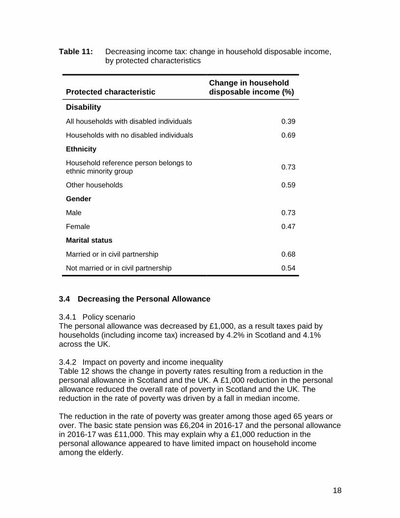
There were small differences in the changes in disposable income across the characteristics set out in Table 11. The decrease across all tax rates appears to have a limited impact on disposable household income when compared with polices such as a citizen’s income. The five-year age group that experienced the largest increase in disposable income was 50-54 year olds (0.77%). This may reflect higher incomes among this age group.

18

Table 11: Decreasing income tax: change in household disposable income, by protected characteristics


Disability



Ethnicity



Gender

Male 0.73

Female 0.47

Marital status



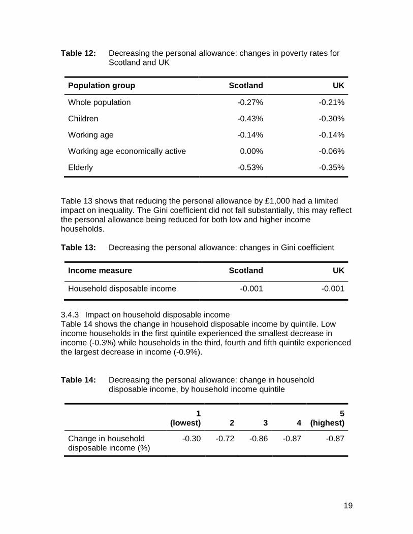
3.4 Decreasing the Personal Allowance 3.4.1 Policy scenario The personal allowance was decreased by £1,000, as a result taxes paid by households (including income tax) increased by 4.2% in Scotland and 4.1% across the UK. 3.4.2 Impact on poverty and income inequality Table 12 shows the change in poverty rates resulting from a reduction in the personal allowance in Scotland and the UK. A £1,000 reduction in the personal allowance reduced the overall rate of poverty in Scotland and the UK. The reduction in the rate of poverty was driven by a fall in median income. The reduction in the rate of poverty was greater among those aged 65 years or over. The basic state pension was £6,204 in 2016-17 and the personal allowance in 2016-17 was £11,000. This may explain why a £1,000 reduction in the personal allowance appeared to have limited impact on household income among the elderly.

19

Table 12: Decreasing the personal allowance: changes in poverty rates for Scotland and UK


Whole population -0.27% -0.21%

Children -0.43% -0.30%

Working age -0.14% -0.14%

Working age economically active 0.00% -0.06%

Elderly -0.53% -0.35%

Table 13 shows that reducing the personal allowance by £1,000 had a limited impact on inequality. The Gini coefficient did not fall substantially, this may reflect the personal allowance being reduced for both low and higher income households. Table 13: Decreasing the personal allowance: changes in Gini coefficient


Household disposable income -0.001 -0.001

3.4.3 Impact on household disposable income Table 14 shows the change in household disposable income by quintile. Low income households in the first quintile experienced the smallest decrease in income (-0.3%) while households in the third, fourth and fifth quintile experienced the largest decrease in income (-0.9%). Table 14: Decreasing the personal allowance: change in household


1 (lowest) 2 3 4

5 (highest)


-0.30 -0.72 -0.86 -0.87 -0.87

20

There were small differences in the changes in household disposable income across the characteristics set out in Table 15. The £1,000 reduction in the personal allowance covers the whole population and would be expected to reduce disposable income across a range of different groups. The five-year age group that experienced the largest decline in household disposable income was 45-49 year olds (-0.91%). This may reflect higher incomes among this age group. Table 15: Decreasing the personal allowance: change in household



Disability



Ethnicity



Gender

Male 0.58

Female 0.41

Marital status



3.5 Increasing the Carer’s Allowance 3.5.1 Policy scenario This scenario considered an increase in carer's allowance of £10 a week. This covered all those who declared being in receipt of it in the FRS (2013/14). 3.5.2 Impact on poverty and income inequality Table 16 shows the change in poverty rates resulting from the increase in carer's allowance. The impact on poverty among the elderly was higher in Scotland compared with the UK as a whole. This may be explained in part by lower

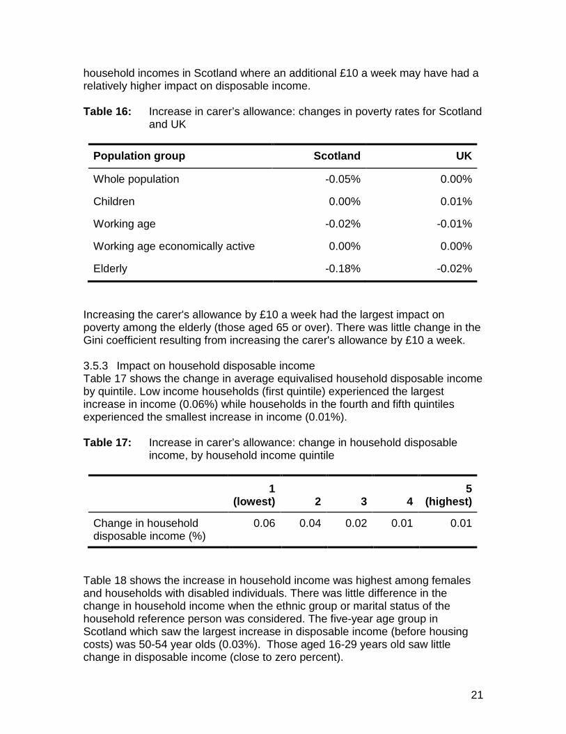
21

household incomes in Scotland where an additional £10 a week may have had a relatively higher impact on disposable income. Table 16: Increase in carer’s allowance: changes in poverty rates for Scotland

and UK


Whole population -0.05% 0.00%




Elderly -0.18% -0.02%

Increasing the carer's allowance by £10 a week had the largest impact on poverty among the elderly (those aged 65 or over). There was little change in the Gini coefficient resulting from increasing the carer's allowance by £10 a week. 3.5.3 Impact on household disposable income Table 17 shows the change in average equivalised household disposable income by quintile. Low income households (first quintile) experienced the largest increase in income (0.06%) while households in the fourth and fifth quintiles experienced the smallest increase in income (0.01%). Table 17: Increase in carer’s allowance: change in household disposable

income, by household income quintile

1 (lowest) 2 3 4

5 (highest)


0.06 0.04 0.02 0.01 0.01

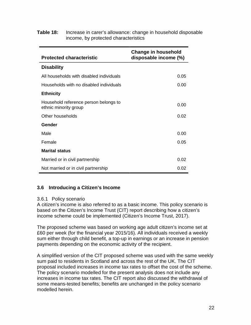
Table 18 shows the increase in household income was highest among females and households with disabled individuals. There was little difference in the change in household income when the ethnic group or marital status of the household reference person was considered. The five-year age group in Scotland which saw the largest increase in disposable income (before housing costs) was 50-54 year olds (0.03%). Those aged 16-29 years old saw little change in disposable income (close to zero percent).

22

Table 18: Increase in carer’s allowance: change in household disposable income, by protected characteristics


Disability



Ethnicity



Gender

Male 0.00

Female 0.05

Marital status



3.6 Introducing a Citizen’s Income 3.6.1 Policy scenario A citizen’s income is also referred to as a basic income. This policy scenario is based on the Citizen’s Income Trust (CIT) report describing how a citizen’s income scheme could be implemented (Citizen’s Income Trust, 2017). The proposed scheme was based on working age adult citizen’s income set at £60 per week (for the financial year 2015/16). All individuals received a weekly sum either through child benefit, a top-up in earnings or an increase in pension payments depending on the economic activity of the recipient. A simplified version of the CIT proposed scheme was used with the same weekly sum paid to residents in Scotland and across the rest of the UK. The CIT proposal included increases in income tax rates to offset the cost of the scheme. The policy scenario modelled for the present analysis does not include any increases in income tax rates. The CIT report also discussed the withdrawal of some means-tested benefits; benefits are unchanged in the policy scenario modelled herein.

23

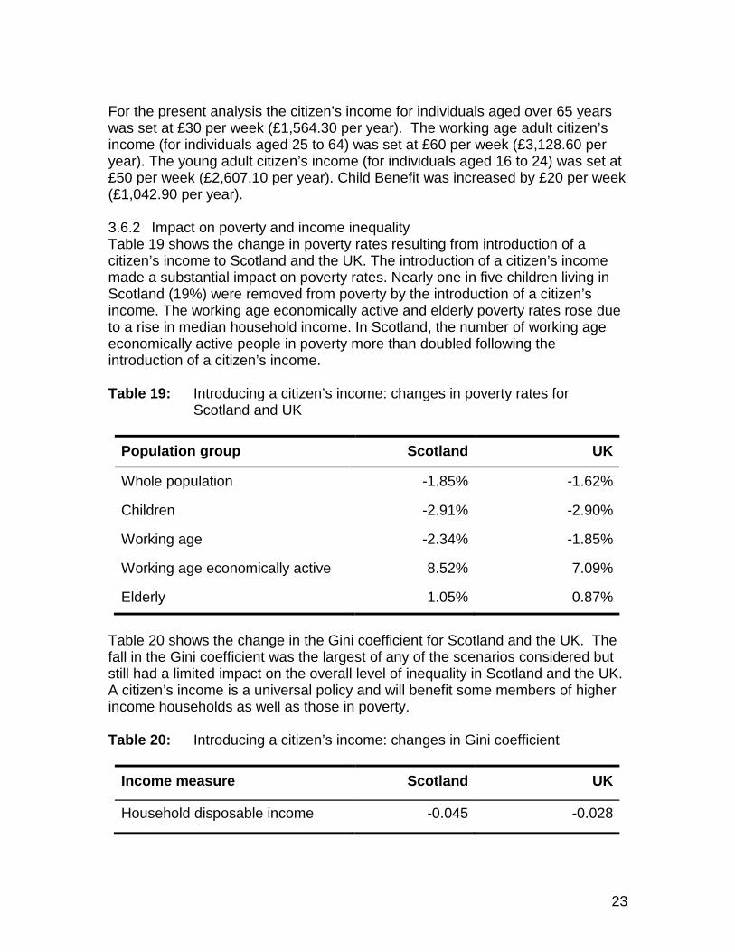
For the present analysis the citizen’s income for individuals aged over 65 years was set at £30 per week (£1,564.30 per year). The working age adult citizen’s income (for individuals aged 25 to 64) was set at £60 per week (£3,128.60 per year). The young adult citizen’s income (for individuals aged 16 to 24) was set at £50 per week (£2,607.10 per year). Child Benefit was increased by £20 per week (£1,042.90 per year). 3.6.2 Impact on poverty and income inequality Table 19 shows the change in poverty rates resulting from introduction of a citizen’s income to Scotland and the UK. The introduction of a citizen’s income made a substantial impact on poverty rates. Nearly one in five children living in Scotland (19%) were removed from poverty by the introduction of a citizen’s income. The working age economically active and elderly poverty rates rose due to a rise in median household income. In Scotland, the number of working age economically active people in poverty more than doubled following the introduction of a citizen’s income. Table 19: Introducing a citizen’s income: changes in poverty rates for

Scotland and UK



Children -2.91% -2.90%



Elderly 1.05% 0.87%

Table 20 shows the change in the Gini coefficient for Scotland and the UK. The fall in the Gini coefficient was the largest of any of the scenarios considered but still had a limited impact on the overall level of inequality in Scotland and the UK. A citizen’s income is a universal policy and will benefit some members of higher income households as well as those in poverty. Table 20: Introducing a citizen’s income: changes in Gini coefficient



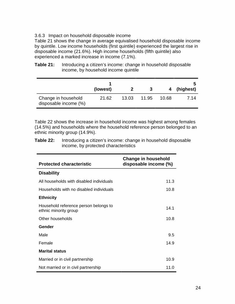
24

3.6.3 Impact on household disposable income Table 21 shows the change in average equivalised household disposable income by quintile. Low income households (first quintile) experienced the largest rise in disposable income (21.6%). High income households (fifth quintile) also experienced a marked increase in income (7.1%). Table 21: Introducing a citizen’s income: change in household disposable

income, by household income quintile

1 (lowest) 2 3 4

5 (highest)


21.62 13.03 11.95 10.68 7.14

Table 22 shows the increase in household income was highest among females (14.5%) and households where the household reference person belonged to an ethnic minority group (14.9%). Table 22: Introducing a citizen’s income: change in household disposable

income, by protected characteristics


Disability



Ethnicity



Gender

Male 9.5

Female 14.9

Marital status



25

3.7 Increasing Council Tax for bands E-H 3.7.1 Policy scenario In this scenario council tax was increased by the following amounts: • Band E: 7.5% • Band F: 12.5% • Band G: 17.5% • Band H: 22.5%

3.7.2 Impact on poverty and income inequality Table 23 shows the change in poverty rates resulting from the above increase in council tax. The rate of poverty fell slightly, overall and for each of the cohorts considered. The impact on poverty among the elderly was slightly higher in Scotland than in the UK as a whole. It is difficult to explain the differences as Scotland operates a different system of council tax to other parts of the UK. However, it is possible that those aged 65 years or over living in Scotland may live in residential properties with higher council tax liabilities (relative to disposable household income). Increasing council tax results in little change in the Gini coefficient. This is perhaps unsurprising given that most households will be liable to pay council tax. Additionally, council tax liabilities are likely to be higher for those households with more disposable income. Table 23: Council tax increased among higher bands: changes in poverty

rates for Scotland and UK



Children -0.13% -0.05%


Working age economically active -0.03% -0.01%

Elderly -0.25% -0.03%

3.7.3 Impact on household disposable income Table 24 shows the change in average equivalised household disposable income by quintile. Higher income households (fifth quintile) experienced the largest reduction in disposable income (-0.21%).

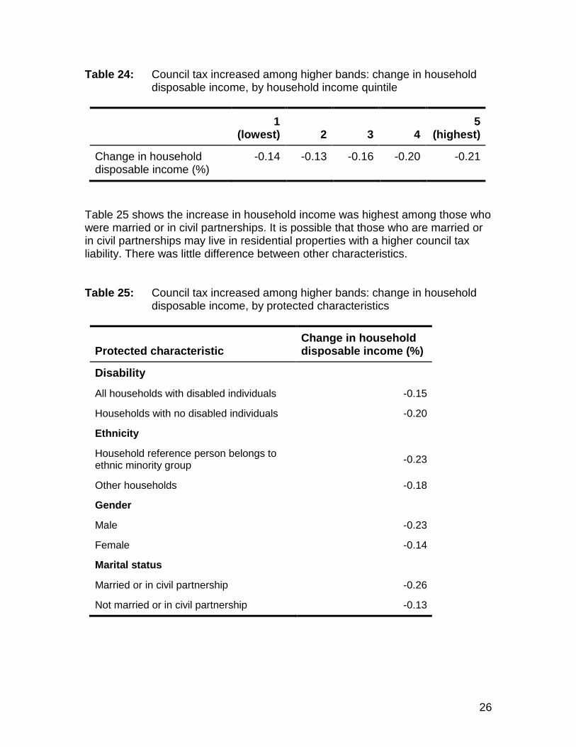
26

Table 24: Council tax increased among higher bands: change in household disposable income, by household income quintile

1 (lowest) 2 3 4

5 (highest)


-0.14 -0.13 -0.16 -0.20 -0.21

Table 25 shows the increase in household income was highest among those who were married or in civil partnerships. It is possible that those who are married or in civil partnerships may live in residential properties with a higher council tax liability. There was little difference between other characteristics. Table 25: Council tax increased among higher bands: change in household



Disability

All households with disabled individuals -0.15

Households with no disabled individuals -0.20

Ethnicity

Household reference person belongs to ethnic minority group -0.23

Other households -0.18

Gender

Male -0.23

Female -0.14

Marital status

Married or in civil partnership -0.26

Not married or in civil partnership -0.13

27

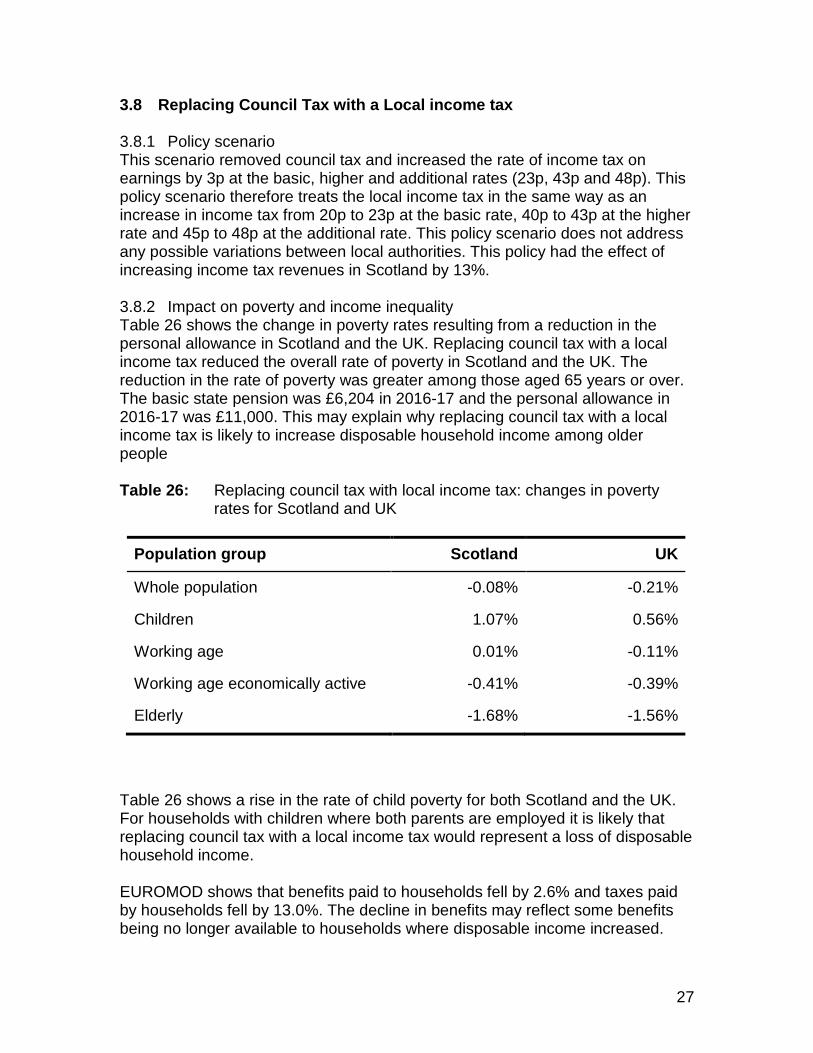
3.8 Replacing Council Tax with a Local income tax 3.8.1 Policy scenario This scenario removed council tax and increased the rate of income tax on earnings by 3p at the basic, higher and additional rates (23p, 43p and 48p). This policy scenario therefore treats the local income tax in the same way as an increase in income tax from 20p to 23p at the basic rate, 40p to 43p at the higher rate and 45p to 48p at the additional rate. This policy scenario does not address any possible variations between local authorities. This policy had the effect of increasing income tax revenues in Scotland by 13%. 3.8.2 Impact on poverty and income inequality Table 26 shows the change in poverty rates resulting from a reduction in the personal allowance in Scotland and the UK. Replacing council tax with a local income tax reduced the overall rate of poverty in Scotland and the UK. The reduction in the rate of poverty was greater among those aged 65 years or over. The basic state pension was £6,204 in 2016-17 and the personal allowance in 2016-17 was £11,000. This may explain why replacing council tax with a local income tax is likely to increase disposable household income among older people Table 26: Replacing council tax with local income tax: changes in poverty

rates for Scotland and UK




Working age 0.01% -0.11%

Working age economically active -0.41% -0.39%

Elderly -1.68% -1.56%

Table 26 shows a rise in the rate of child poverty for both Scotland and the UK. For households with children where both parents are employed it is likely that replacing council tax with a local income tax would represent a loss of disposable household income. EUROMOD shows that benefits paid to households fell by 2.6% and taxes paid by households fell by 13.0%. The decline in benefits may reflect some benefits being no longer available to households where disposable income increased.

28

The net effect of this policy increased total equivalised household disposable income in Scotland by 1.9%, the equivalent figure for the UK was 1.6%. This suggests that income tax rates in Scotland would need to rise by more than 3% for the policy to be revenue neutral. Table 27 shows that replacing council tax with a local income tax reduced the Gini coefficient. However, the decline in inequality was modest. Table 27: Replacing council tax with local income tax: changes in Gini

coefficient



3.8.3 Impact on household disposable income Table 28 shows the change in average equivalised household disposable income by quintile. Low income households (first quintile) experienced the largest increase in income (4.7%) while households in the fifth quintile also experienced an increase in disposable income, albeit a more modest one (0.9%). Table 28: Replacing council tax with local income tax: change in household


1 (lowest) 2 3 4

5 (highest)


4.74 3.67 3.04 1.83 0.08

Table 29 sets out differences in the changes in disposable income by protected characteristics. Households with disabled individuals experienced the largest increase in disposable household income (2.25%). The age group that experienced the largest rise in disposable income were those aged 75 years or over (3.7%). This may reflect lower household incomes among this group.

29

Table 29: Replacing council tax with local income tax: change in household disposable income, by protected characteristics


Disability



Ethnicity



Gender

Male 1.98

Female 1.60

Marital status



3.9 Impact on taxes paid and benefits received Information on the costs associated with the scenarios is set out in the accompanying Microsoft Excel workbook. EUROMOD produces a wide range of indicators related to taxes, benefits and income, providing an indication of the main direction of change and broad scale of change. The policy scenarios that were a net cost to the public purse were: basic rate of income tax decreased by 1p, carer’s allowance increase, introducing a citizen’s income, decreasing income tax by 1p (all rates), council tax replaced by a local income tax and increasing the personal allowance. The policy scenarios that were a net benefit to the public purse were: council tax increase, decreasing the personal allowance, basic rate of income tax increased by 5p, higher rate of income tax increased by 5p and wealth tax introduction.

30

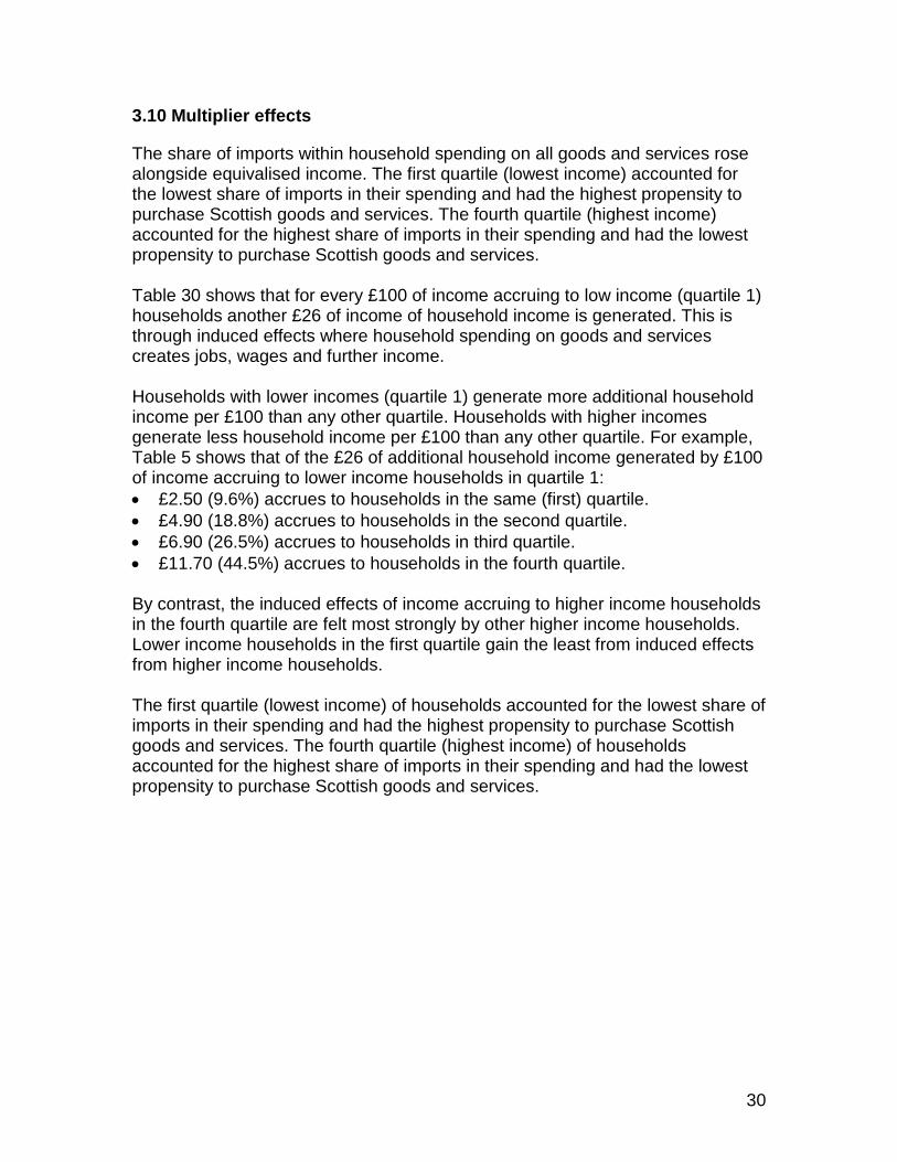
3.10 Multiplier effects

The share of imports within household spending on all goods and services rose alongside equivalised income. The first quartile (lowest income) accounted for the lowest share of imports in their spending and had the highest propensity to purchase Scottish goods and services. The fourth quartile (highest income) accounted for the highest share of imports in their spending and had the lowest propensity to purchase Scottish goods and services. Table 30 shows that for every £100 of income accruing to low income (quartile 1) households another £26 of income of household income is generated. This is through induced effects where household spending on goods and services creates jobs, wages and further income. Households with lower incomes (quartile 1) generate more additional household income per £100 than any other quartile. Households with higher incomes generate less household income per £100 than any other quartile. For example, Table 5 shows that of the £26 of additional household income generated by £100 of income accruing to lower income households in quartile 1: • £2.50 (9.6%) accrues to households in the same (first) quartile. • £4.90 (18.8%) accrues to households in the second quartile. • £6.90 (26.5%) accrues to households in third quartile. • £11.70 (44.5%) accrues to households in the fourth quartile. By contrast, the induced effects of income accruing to higher income households in the fourth quartile are felt most strongly by other higher income households. Lower income households in the first quartile gain the least from induced effects from higher income households. The first quartile (lowest income) of households accounted for the lowest share of imports in their spending and had the highest propensity to purchase Scottish goods and services. The fourth quartile (highest income) of households accounted for the highest share of imports in their spending and had the lowest propensity to purchase Scottish goods and services.

31

Table 30: Impact of multiplier effects on additional £100 of household disposable income, by household income quartile

Impact on household

income

Lowest income quartile

receives £100

Income quartile 2 receives

£100

Income quartile 3 receives

£100

Highest income quartile

receives £100

1 (lowest) £102.5 £2.1 £1.7 £1.5

2 £4.9 £104.1 £3.3 £3.1

3 £6.9 £5.9 £104.6 £4.3

4 (highest) £11.7 £9.9 £7.8 £107.2

Total impact £126.0 £121.9 £117.4 £116.1

3.11 Summary of findings The results of modelling the policy scenarios were presented, including a wide range of indicators of poverty, inequality and income distribution. The indicators are useful in setting out the effectiveness of policies in raising incomes for different groups. A summary of the change in household disposable income by household income quintile is set out in Table 31. All of the scenarios outlined in this section are included in the accompanying Microsoft Excel workbook.

32

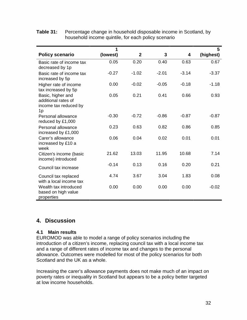
Table 31: Percentage change in household disposable income in Scotland, by household income quintile, for each policy scenario

Policy scenario 1

(lowest) 2 3 4 5

(highest) Basic rate of income tax decreased by 1p

0.05 0.20 0.40 0.63 0.67

Basic rate of income tax increased by 5p

-0.27 -1.02 -2.01 -3.14 -3.37

Higher rate of income tax increased by 5p

0.00 -0.02 -0.05 -0.18 -1.18

Basic, higher and additional rates of income tax reduced by 1p

0.05 0.21 0.41 0.66 0.93

Personal allowance reduced by £1,000

-0.30 -0.72 -0.86 -0.87 -0.87

Personal allowance increased by £1,000

0.23 0.63 0.82 0.86 0.85

Carer’s allowance increased by £10 a week

0.06 0.04 0.02 0.01 0.01

Citizen's income (basic income) introduced

21.62 13.03 11.95 10.68 7.14

Council tax increase -0.14 0.13 0.16 0.20 0.21

Council tax replaced with a local income tax

4.74 3.67 3.04 1.83 0.08

Wealth tax introduced based on high value properties

0.00 0.00 0.00 0.00 -0.02

4. Discussion 4.1 Main results EUROMOD was able to model a range of policy scenarios including the introduction of a citizen’s income, replacing council tax with a local income tax and a range of different rates of income tax and changes to the personal allowance. Outcomes were modelled for most of the policy scenarios for both Scotland and the UK as a whole. Increasing the carer’s allowance payments does not make much of an impact on poverty rates or inequality in Scotland but appears to be a policy better targeted at low income households.

33

The introduction of a citizen’s income (with no other changes to the tax and benefit system) was modelled to have the largest impact on disposable incomes among low income households. After the citizen’s income, the policy scenario that had the largest impact on low income households was the replacement of council tax with a local income tax. The overall effect of replacing council tax with a local income tax increased total equivalised household disposable income in Scotland by 1.9%, compared with 10.9% in the citizen’s income scenario. A higher proportion of the additional household income arising from the introduction of a citizen’s income accrues to households outside the lowest household income quintile (compared to the local income tax scenario). However, the introduction of a citizen’s income results in the largest reduction in income inequality. Introducing a citizen’s income and replacing council tax with a local income tax were also the most expensive policy scenarios. In both scenarios, the increase in household income reflects the additional public spending associated with each policy. The relative poverty rates suggest that the introduction of a citizen’s income would markedly raise disposable income levels for low income households. However, this policy is likely to be of limited benefit for those in work, measured by the working age economically active population. Indeed, some people already in work would move into relative poverty. Similarly, replacing council tax with a local income tax had the effect of moving children into relative poverty. The policy provided the largest increase in disposable income for those 65 years of age or older, those aged 16-24 years also enjoyed a sizeable increase in disposable income. For households with children where both parents are employed it is likely that replacing council tax with a local income tax would represent a loss of disposable household income. The policy scenarios modelled here show that efforts to increase disposable household income among Scotland’s low income households may also increase disposable household income among higher income households. Increasing the carer’s allowance payments does not make much of an impact on poverty rates or inequality in Scotland but appears to be a policy better targeted at low income households. Changes in the rate of income tax are useful in demonstrating the relative impact of the basic, higher and additional rates of income tax. Raising the basic rate of income tax by 1p has a higher impact on higher income households in Scotland than raising the higher or additional rate of income tax by 1p. This is because the number of households paying income tax at the higher or additional rates is relatively small.

34

The inclusion of multiplier effects allowed the impact of long term changes in disposable household income on the wider Scottish economy to be assessed. The multiplier effects provide evidence both of ‘trickle up’ effects where income and spending from low income households benefit higher income households. The multiplier effects broadly have the effect of making interventions more cost effective, for example replacing council tax with a local income tax becomes broadly cost neutral. The multiplier effects also have the effect of reducing the impact of interventions on inequality. 4.2 Limitations 4.2.1 Limitations of EUROMOD and FRS EUROMOD cannot produce a fully comprehensive analysis. The main limitations of EUROMOD are threefold. First, the modelling is limited by the information available in the input dataset. If the information required in order to calculate a tax requirement or a benefit eligibility for an individual or household is not available in the input dataset, it cannot be modelled. Some taxes and benefits are beyond the scope of EUROMOD entirely and are neither included in the input or the output dataset. For instance, there is no variable linked to Value Added Tax (VAT) charged to individuals or companies. Other variables cannot be accurately simulated with the available data and are included in the datasets, but the rules governing them may not be changed by the model. For example, the FRS includes a question on whether the respondent is in receipt of Carer’s Allowance. Basic modelling can be done around this, for example Carer’s Allowance can be increased by 10% for everyone over the age of 70 years, but the eligibility criteria cannot be changed in detail, for example Carer’s Allowance is dependent on the benefits received by the person being cared for. This condition cannot be modified directly in EUROMOD as there are no data on the individual that a carer provides care to. Furthermore, the modelling depends on how well the FRS represents the population. Like all “weighted” population surveys, FRS data are scaled up to represent the overall population. The Office for National Statistics (ONS) provide weights for each household in the FRS, with each household representing about 600 households. Although the sample size of the FRS survey data is large by international standards, care should still be taken in interpreting results for small sub-groups of the population. Certain groups and income types are known to be underrepresented such as the number of high-income taxpayers, self-

35

employment earnings and investment income. This compromises the accuracy of modelling on these groups. ISER makes minor adjustments to the FRS in order to maximize the usability of the FRS. Some values are artificially assigned or “imputed”. Variables subject to this include but are not limited to: • Mortgage interest, which is estimated for people where a single repayment

amount includes both interest and capital repayment. • Rent is calculated to be gross although in some cases housing benefit has

been deducted from reported rent. • The regime under which individuals pay National Insurance contributions is

estimated from information on gross earnings and the contribution payment. • The categorization of state pension as the FRS data only includes one

variable covering all state pension payments. • Council Tax: only about 20% report the amount of council tax (gross of

council tax benefit) so it needs to be imputed for the other 80%. The FRS does include a variable for council tax band.

• Income support for carers. • Increase in female pension age. The second reason why EUROMOD cannot produce a fully comprehensive analysis is that the model is static, which means it does not include behavioural responses. For instance, raising taxes may cause a change in the labour supply, and while this potential effect can be included in the modelling, it is beyond the scope of EUROMOD as a standalone model. In addition EUROMOD is a microsimulation model, it does not simulate the effects of a policy change on macroeconomic variables such as trade, productivity and employment. Nevertheless, from 2017 the input dataset will include information on household expenditure, which will allow for some modelling of indirect taxes such as VAT and excise duties. 4.2.2 Policy scenarios Citizen’s Income, also referred to as Citizen’s Basic Income and Universal Basic Income, has received a lot of academic and policy attention in recent years. The Citizen’s Income modelled in this report was simplistic as no other changes to the tax and benefit system were made. This was a deliberate choice to illustrate the likely direction of the effect on household disposable income across household income quintiles. The Institute of Public Policy Research has evaluated the impact of Citizen’s Income scenarios that would be deemed ‘cost-neutral’ through tax and benefit adjustments (Martinelli, 2017). Although the scale of household income change would be less marked, the cost-neutral policies were progressive with lower income households in the UK, on average, gaining the most. This, in turn, leads to a reduction in income inequalities. However, the report also emphasises that for a significant minority of lower income households their base income would fall.

36

Replacing council tax with a local income tax was another policy that had large impacts on household disposable income in our modelling, particularly for lower income households. This was considered an alternative to the current property-based council tax in Scotland by the Commission on Local Tax Reform in Scotland (2015). However, it was identified that in practical terms it would be challenging for savings, investment and dividend income to be subject to local tax meaning some high-wealth individuals with substantial unearned income would pay little or no tax. In addition, it was highlighted that such a system may be problematic as it would not take into account income after necessary costs, such as caring for children or those with a disability. The Commission concluded that a replacement council tax would benefit from including multiple forms of tax, including income tax, to ensure fairness. Although multiple forms of tax mechanisms were not modelled in this study for the replacement of council tax, the local income tax modelled provides a useful illustration of the potential impact of alternative approaches in Scotland. 4.3 Recommendations This research project sought to provide an opportunity for users to access the tax-benefit model directly. This would allow further policy scenarios on taxes and benefits to be modelled with outcomes updated accordingly. The modelled scenarios outlined in this report can be expanded on with a modest commitment from NHS Health Scotland to develop some capacity to use EUROMOD.

37

5. References Aarbu, K. & Thoreson, T. (2001) “Income Responses to Tax Changes: Evidence from the Norwegian Tax Reform," National Tax Journal, 54(2): pp319-334. Adam, S. (2012). The IFS Green Budget. [online] Institute for Fiscal Studies. Available at: https://www.ifs.org.uk/budgets/gb2012/gb2012.pdf (Accessed 1 Mar. 2017). Auten, G. and Carroll, R. (1999). The Effect of Income Taxes on Household Income. Review of Economics and Statistics, 81(4), pp.681-693. Auten, G., Carroll, R. and Gee, G. (2008). The 2001 and 2003 Tax Rate Reductions: An Overview and Estimate of the Taxable Income Response. National Tax Journal, 61(3), pp.345-364. Bell, D. (2015). Behavioural responses to changes in income tax rates: What Will Happen in Scotland? [online] Evidence to the Scottish Parliament Finance Committee. Available at: http://www.parliament.scot/S4_FinanceCommittee/General%20Documents/David_Bell_briefing.pdf (Accessed 1 Mar. 2017). Blow, L. and Preston, I. (2002) Deadweight Loss and Taxation of Earned Income: Evidence from Tax Records of the UK Self-Employed, IFS Working Paper No. 02/15. Blundell, R., Duncan, A., and Meghir, C. (1998) Estimating Labour supply responses using tax reforms, in Econometrica Vol. 66, No.4 Blundell, R. and MaCurdy T. (1999) Labour supply: a review of alternative approaches. In: Ashenfelter, O. Card, D. (eds). Handbook of Labour Economics, Vol. 3. Available at: http://www.ucl.ac.uk/~uctp39a/Blundell-MaCurdy-1999.pdf (Accessed 1 Mar. 2017) Brewer, M., Saez, E. and Shephard, A. (2010). Means-testing and Tax Rates on Earnings, The Mirrlees Review: Reforming the Tax System for the 21st Century, [online] IFS. Available at: http://www.ifs.org.uk/uploads/mirrleesreview/dimensions/ch2.pdf (Accessed 1 Mar. 2017). Browne, J. (2015). The Impact of Proposed Tax, Benefit and Minimum Wage Reforms on Household Incomes and Work incentives, (Online) Institute for Fiscal Studies. Available at: https://www.ifs.org.uk/uploads/publications/comms/R111.pdf (Accessed 1 Mar. 2017)

https://www.ifs.org.uk/budgets/gb2012/gb2012.pdf

http://www.parliament.scot/S4_FinanceCommittee/General%20Documents/David_Bell_briefing.pdf

http://www.parliament.scot/S4_FinanceCommittee/General%20Documents/David_Bell_briefing.pdf

http://www.ucl.ac.uk/%7Euctp39a/Blundell-MaCurdy-1999.pdf

http://www.ifs.org.uk/uploads/mirrleesreview/dimensions/ch2.pdf

https://www.ifs.org.uk/uploads/publications/comms/R111.pdf

38

Brulhart et al. (2016) Cesifo Working Paper No. 5966, Taxing Wealth: Evidence from Switzerland. Available at: http://www.nber.org/papers/w22376 (Accessed 1 Mar. 2017) Carroll, R., and Hrung, W. (2005) ‘What Does the Taxable Income Elasticity Say about Dynamic Responses to Tax Changes?’, American Economic Review, 95, pp426–31. Chetty, R. (2009) ‘Bounds on Elasticities with Optimization Frictions: A Synthesis of Micro and Macro Evidence on Labour Supply’, National Bureau of Economic Research (NBER), Working Paper 15616. Available at: http://www.nber.org/papers/w15616 (Accessed 1 Mar. 2017) Chetty, R. Friedman, J. Olsen, T., & Pistaferri, L. (2011) Adjustment Costs, Firm Responses, and Micro vs. Macro Labour Supply Elasticities: Evidence from Danish Tax. Available at: https://dash.harvard.edu/bitstream/handle/1/9639984/Friedman-AdjustmentCosts.pdf?sequence=1 (Accessed 1 Mar. 2017) Citizen’s Income Trust (2017) Citizen’s Basic Income A Brief Introduction. Available at: http://citizensincome.org/wp-content/uploads/2016/03/Citizens-Basic-Income-FINAL_WEB.pdf (Accessed 1 Mar. 2017) Commission on Local Tax Reform. (2015) Just Change: A New Approach to Local Taxation. APS Group. Cullen, J., & Roger G. (2007) “Taxes and Entrepreneurial Risk-Taking: Theory and Evidence in the U.S.,” Journal of Public Economics. 91(7-8): pp1479- 1505. Feldstein, M. (1995) The effect of marginal tax rates on taxable income: a panel study of the 1986 Tax Reform Act. Journal of Political Economy 103 (3), pp551-572 Gentry, W. & Glenn H., (2000) Tax Policy and Entrepreneurial Entry, American Economic Review 90(2): pp283-287. Giertz, S (2005) “A Sensitivity Analysis of the Elasticity of Taxable Income”, CBO Working Paper 2005-01 Giertz, S. (2010) The Elasticity of Taxable Income during the 1990s: New Estimates and Sensitivity Analyses, Economics Department Faculty Publications, Economic Department. Available at: http://digitalcommons.unl.edu/cgi/viewcontent.cgi?article=1069&context=econfacpub (Accessed 1 Mar. 2017)

http://www.nber.org/papers/w22376


https://dash.harvard.edu/bitstream/handle/1/9639984/Friedman-AdjustmentCosts.pdf?sequence=1

https://dash.harvard.edu/bitstream/handle/1/9639984/Friedman-AdjustmentCosts.pdf?sequence=1

http://citizensincome.org/wp-content/uploads/2016/03/Citizens-Basic-Income-FINAL_WEB.pdf

http://citizensincome.org/wp-content/uploads/2016/03/Citizens-Basic-Income-FINAL_WEB.pdf

http://digitalcommons.unl.edu/cgi/viewcontent.cgi?article=1069&context=econfacpub

http://digitalcommons.unl.edu/cgi/viewcontent.cgi?article=1069&context=econfacpub

39

Goolsbee, A., (2000) “What happens when you tax the rich? Evidence from executive compensation.” Journal of Political Economy 108(2), pp352-378. Gruber, J. & Saez, E. (2002) The Elasticity of Taxable Income: Evidence and Implications, Journal of Public Economics, 84, pp1-32 Heckman, J. Lochner, L., & Taber, C. (1999) ‘General Equilibrium Cost Benefit Analysis of Education and Tax Policies’, in G. Ranis and L. Raut (eds), Trade Development and Growth: Essays in Honor of T. N. Srinivasan, Amsterdam: Elsevier Publishers. HMRC (2015) Disaggregation of HMRC tax receipts. UK Government. Available at: https://www.gov.uk/government/statistics/disaggregation-of-hmrc-tax-receipts#history (Accessed 1 Mar. 2017) Johnson, P & Phillips, D. (2014), 50p tax – strolling across the summit of the Laffer curve? Institute for Fiscal Studies. Available at: https://www.ifs.org.uk/publications/7066 (Accessed 1 Mar. 2017) Kopczuk, W. (2005), ‘Tax Bases, Tax Rates and the Elasticity of Reported Income’, Journal of Public Economics, 89, pp2093–119. Kopczuk, W. (2010) ‘Economics of Estate Taxation: A Brief Review of Theory and Evidence’, National Bureau of Economic Research (NBER), Working Paper 15741. Available at: www.nber.org/papers/w15741 (Accessed 1 Mar. 2017) Kose, M., Prasa, E. and Terrones M. (2008) Does Openness to International Financial Flows Raise Productivity Growth? IMF Working Paper, Research Department, WP/08/242. Available at: http://ec.europa.eu/economy_finance/events/2008/20081016/kose_p.pdf (Accessed 1 Mar. 2017) Lindsey, L. (1987) Individual Taxpayer Response to Tax Cuts: 1982-1984, with Implications for the Revenue Maximizing Tax Rate, Journal of Public Economics, 33(2): pp173-61 206 Long, J. (1999) The Impact of Marginal Tax Rates on Taxable Income: Evidence from State Income Tax Differentials. Southern Economic Journal 65(4): pp855-869. Martinelli, L. (2017) Exploring the Distributional and Work Incentive Effects of Plausible Illustrative Basic Income Schemes. Institute of Public Policy Research, University of Bath. Available at: http://www.bath.ac.uk/publications/exploring-the-distributional-work-incentive-effects-of-plausible-illustrative-basic-income-schemes/attachments/Luke_WP2_Web.pdf

https://www.gov.uk/government/statistics/disaggregation-of-hmrc-tax-receipts#history

https://www.gov.uk/government/statistics/disaggregation-of-hmrc-tax-receipts#history

https://www.ifs.org.uk/publications/7066


http://ec.europa.eu/economy_finance/events/2008/20081016/kose_p.pdf

40

McNicoll, I. & McLellan, D. (2003) Extensions to the Scottish Input-Output Modelling System: A Disaggregation of the Household Sector, Scottish Economic Statistics. Meade, J. (1978), The Structure and Reform of Direct Taxation: Report of a Committee Chaired by Professor J. E. Meade for the Institute for Fiscal Studies, London: George Allen & Unwin. Available at: http://www.ifs.org.uk/publications/3433 (Accessed 1 Mar. 2017) Milligan, K. & Smart, M. (2016) Taxation and top incomes in Canada. Available at: http://homes.chass.utoronto.ca/~msmart/cje-3.pdf (Accessed 1 Mar. 2017) Mirrlees J., Adam S., Besley T., Blundell R., Bond S., Chote R., Gammie M., Johnson P., Myles G. & Poterba J. (2011) Institute for Fiscal Studies, Tax by design, Oxford University Press. Available at: https://www.ifs.org.uk/publications/5353 (Accessed 1 Mar. 2017) OECD (2010) Tax Policy Reform and Economic Growth, OECD Publishing. Available at: http://www.oecd.org/ctp/tax-policy/tax-policy-reform-and-economic-growth-9789264091085-en.htm (Accessed 1 Mar. 2017) OECD (2012) Tax Effects on Foreign Direct Investment, Policy Brief. Available at: https://www.oecd.org/investment/investment-policy/40152903.pdf (Accessed 1 Mar. 2017) Saez, E. (2001) Using Elasticities to Derive Optimal Tax Rates, Review of Economic Studies, Vol. 68 Saez, E. (2004) Reported Incomes and Marginal Tax Rates, 1960-2000: Evidence and Policy Implications”, NBER Working Paper No.10273, National Bureau of Economic Research. Saez, E., Slemrod, J., & Giertz, S. (2009) The Elasticity of Taxable Income with Respect to Marginal Tax Rates: A Critical Review. Available at: http://www.nber.org/papers/w15012.pdf (Accessed 1 Mar. 2017) Saez, E. (2016) Taxing the Rich More: Preliminary Evidence from the 2013 Tax Increase. Available at: http://eml.berkeley.edu/~saez/saezNBERWP16TPE.pdf (Accessed 1 Mar. 2017) Scottish Enterprise (2014) Scottish Enterprise Economic Impact Guidance. Available at: http://www.evaluationsonline.org.uk/evaluations/Documents.do?action=download&id=693 (Accessed 1 Mar. 2017) Scottish Government (2015) Input-Output Methodology Guide.

http://www.ifs.org.uk/publications/3433

http://homes.chass.utoronto.ca/%7Emsmart/cje-3.pdf

http://www.ifs.org.uk/people/profile/203


http://www.lse.ac.uk/economics/people/facultyPages/TimBesley.aspx#DynamicJumpMenuManager_1_Anchor_3





http://economics.mit.edu/faculty/poterba

https://www.ifs.org.uk/publications/5353

http://www.oecd.org/ctp/tax-policy/tax-policy-reform-and-economic-growth-9789264091085-en.htm

http://www.oecd.org/ctp/tax-policy/tax-policy-reform-and-economic-growth-9789264091085-en.htm

https://www.oecd.org/investment/investment-policy/40152903.pdf

http://www.nber.org/papers/w15012.pdf

http://eml.berkeley.edu/%7Esaez/saezNBERWP16TPE.pdf

http://www.evaluationsonline.org.uk/evaluations/Documents.do?action=download&id=693

http://www.evaluationsonline.org.uk/evaluations/Documents.do?action=download&id=693

41

Scottish Government (2016a) 2013 Input-Output Tables. Scottish Government (2016b) The impact of an increase in the additional rate of income tax from 45p to 50p Scotland. Available at: http://www.gov.scot/Resource/0049/00497818.pdf (Accessed 1 Mar. 2017) Scottish Public Health Observatory. (2014) Informing investment to reduce inequalities: a commentary. Edinburgh; ScotPHO. Available at: http://www.scotpho.org.uk/comparative-health/health-inequalities-tools/informing-investment-to-reduce-health-inequalities-iii (Accessed 1 Mar. 2017) Selen, J (2002) “Taxable income response to tax changes: Evidence from the 1990/91 Swedish Tax Reform," FIEF Working Paper No. 177. Sianesi, B & Reenen, J. (2000). The Returns to Education: A Review of the Macro-Economic Literature. Available at: http://cee.lse.ac.uk/ceedps/ceedp06.pdf (Accessed 1 Mar. 2017) Slemrod, J. (1998) Methodological issues in measuring and interpreting taxable income elasticities. National Tax Journal 51 (4), pp773–788. Slemrod, J. and Kopczuk, W. (2002) “The optimal elasticity of taxable income,” Journal of Public Economics 84 (2002) pp91–112. Available at: http://www.ucl.ac.uk/~uctp39a/Slemrod_Kopczuk_2002_Journal-of-Public-Economics.pdf (Accessed 1 Mar. 2017) UK Government. (2009) Budget 2009, Building Britain’s future, Economic and Fiscal Strategy Report and Financial Statement and Budget Report. Available at: http://webarchive.nationalarchives.gov.uk/20130129110402/http:/www.hm-treasury.gov.uk/d/bud09_completereport_2520.pdf (Accessed 1 Mar. 2017) UK Government (2010) Budget 2010, Securing the Recovery, Economic and Fiscal Strategy Report and Financial Statement and Budget Report. Available at: http://webarchive.nationalarchives.gov.uk/20100413203226/http:/www.hm-treasury.gov.uk/d/budget2010_complete.pdf (Accessed 1 Mar. 2017) UK Government (2012) The Exchequer effect of the 50 per cent additional rate of income tax, HMRC. Available at: http://webarchive.nationalarchives.gov.uk/20130129110402/http:/www.hmrc.gov.uk/budget2012/excheq-income-tax-2042.pdf (Accessed 1 Mar. 2017)

http://www.gov.scot/Resource/0049/00497818.pdf

http://www.scotpho.org.uk/comparative-health/health-inequalities-tools/informing-investment-to-reduce-health-inequalities-iii

http://www.scotpho.org.uk/comparative-health/health-inequalities-tools/informing-investment-to-reduce-health-inequalities-iii

http://cee.lse.ac.uk/ceedps/ceedp06.pdf

http://www.ucl.ac.uk/%7Euctp39a/Slemrod_Kopczuk_2002_Journal-of-Public-Economics.pdf

http://www.ucl.ac.uk/%7Euctp39a/Slemrod_Kopczuk_2002_Journal-of-Public-Economics.pdf

http://webarchive.nationalarchives.gov.uk/20130129110402/http:/www.hm-treasury.gov.uk/d/bud09_completereport_2520.pdf

http://webarchive.nationalarchives.gov.uk/20130129110402/http:/www.hm-treasury.gov.uk/d/bud09_completereport_2520.pdf

http://webarchive.nationalarchives.gov.uk/20100413203226/http:/www.hm-treasury.gov.uk/d/budget2010_complete.pdf

http://webarchive.nationalarchives.gov.uk/20100413203226/http:/www.hm-treasury.gov.uk/d/budget2010_complete.pdf

http://webarchive.nationalarchives.gov.uk/20130129110402/http:/www.hmrc.gov.uk/budget2012/excheq-income-tax-2042.pdf

http://webarchive.nationalarchives.gov.uk/20130129110402/http:/www.hmrc.gov.uk/budget2012/excheq-income-tax-2042.pdf

42

Appendix 1: Taxes, benefits and modelling in EUROMOD Taxes/National Insurance contributions Income Tax Modelled: Yes Notes: The number of taxpayers is overestimated by 3% (basic rate

taxpayers: 6%; higher: 14% and additional: 38%). Revenue is underestimated by 16% (basic rate tax: no discrepancy; higher rate 13% and more than 60% for the additional rate). This is because there is some underreporting of high incomes and an under-representation in the FRS of high-income taxpayers.

National Insurance contributions Modelled: Yes Notes: Number of contributors was underestimated by 19% in

EUROMOD (in 2008 – latest data available). Employee and employer revenue are underestimated by 15% only (in 2015). Self-employed contributions however are over-estimated by 54% (in 2012). Special schemes for small groups of people are ignored in the modelling.

Council Tax Modelled: Included but not simulated Notes: The number of taxpayers is probably slightly overestimated in

the FRS. Gross Council Tax revenue is well estimated (in 2012). Comparison with external figures must consider that later years are net of Council tax benefit/support whereas EUROMOD figures remain gross. It is not simulated because there are no data on the property value and no local information below the standard region (which would become an issue if local authorities in Scotland no longer maintained the freeze).

Capital Gains Tax Modelled: No Notes: No information on asset sales in FRS Inheritance Tax Modelled: No Notes: No information on receipt of an estate in FRS Stamp Duty and Stamp Duty Land Tax Modelled: No

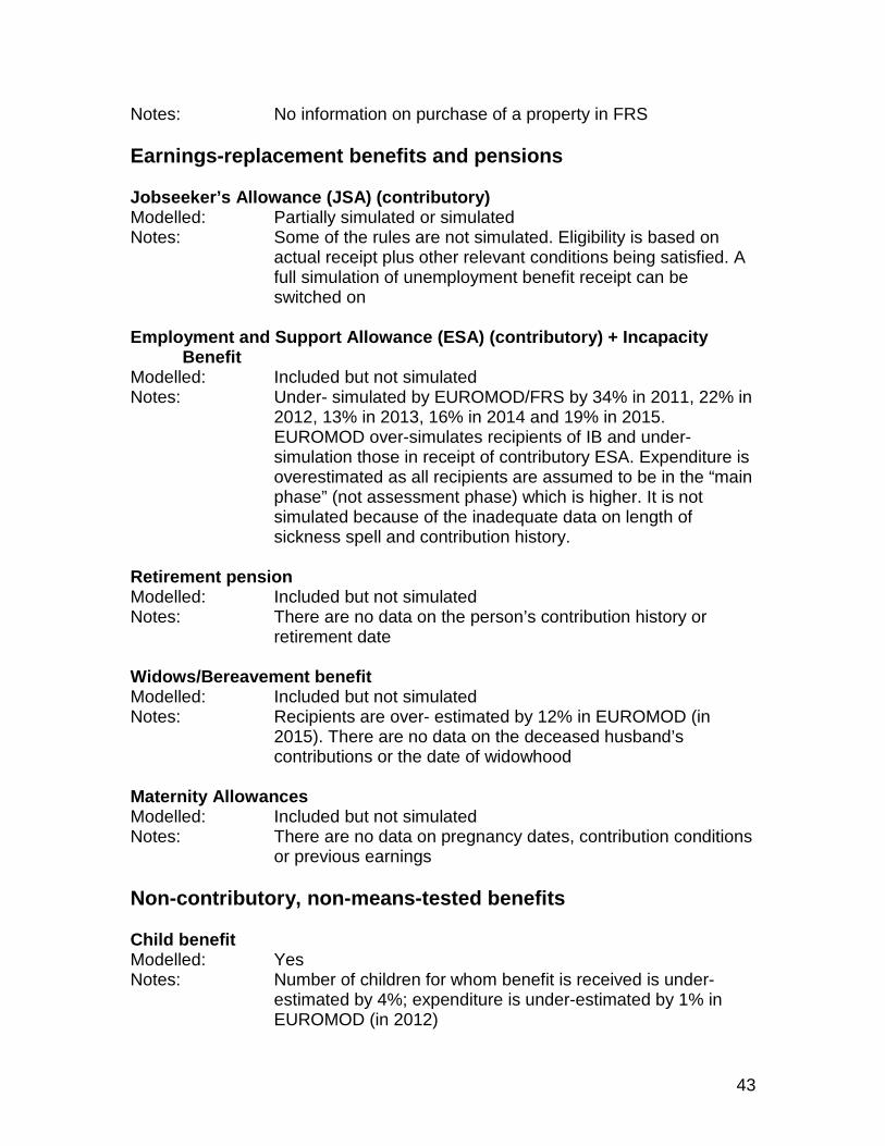
43

Notes: No information on purchase of a property in FRS Earnings-replacement benefits and pensions Jobseeker’s Allowance (JSA) (contributory) Modelled: Partially simulated or simulated Notes: Some of the rules are not simulated. Eligibility is based on

actual receipt plus other relevant conditions being satisfied. A full simulation of unemployment benefit receipt can be switched on

Employment and Support Allowance (ESA) (contributory) + Incapacity

Benefit Modelled: Included but not simulated Notes: Under- simulated by EUROMOD/FRS by 34% in 2011, 22% in

2012, 13% in 2013, 16% in 2014 and 19% in 2015. EUROMOD over-simulates recipients of IB and under-simulation those in receipt of contributory ESA. Expenditure is overestimated as all recipients are assumed to be in the “main phase” (not assessment phase) which is higher. It is not simulated because of the inadequate data on length of sickness spell and contribution history.

Retirement pension Modelled: Included but not simulated Notes: There are no data on the person’s contribution history or

retirement date Widows/Bereavement benefit Modelled: Included but not simulated Notes: Recipients are overestimated by 12% in EUROMOD (in

2015). There are no data on the deceased husband’s contributions or the date of widowhood

Maternity Allowances Modelled: Included but not simulated Notes: There are no data on pregnancy dates, contribution conditions

or previous earnings Non-contributory, non-means-tested benefits Child benefit Modelled: Yes Notes: Number of children for whom benefit is received is under-

estimated by 4%; expenditure is under-estimated by 1% in EUROMOD (in 2012)

44

Attendance Allowance Modelled: Included but not simulated Notes: Recipients are under-reported in the FRS by 50%. There is

insufficient information on the person’s disability to simulate it. Disability Living Allowance + Personal Independence Payment Modelled: Included but not simulated Notes: EUROMOD underestimates number of recipients by 1% after

adjustment (in 2015). There is insufficient information on the person’s disability to simulate it.

Severe Disability Allowance (SDA) Modelled: Included but not simulated Notes: Recipients under-reported in the FRS, perhaps because of

respondent confusion between SDA and the disability premia in the Pension Credit. There is insufficient information on the person’s disability to simulate it.

Carer’s Allowance Modelled: Included but not simulated Notes: Recipients are underestimated by 29% (in 2015). There is

insufficient information on the disability of the person being cared for to simulate it.

Industrial Injuries Disablement Benefit Modelled: Included but not simulated Notes: There is insufficient information on the person’s disability to

simulate it. Guardian’s Allowance Modelled: No Notes: There is no information linking the respondent to a child they

may be caring for. War Pension and allowances Modelled: Included but not simulated Notes: There is no information on past circumstances. Winter fuel allowance Modelled: Yes Notes: Number of recipients overestimated by 3%; expenditure is

under-estimated by 2% (in 2015).

45

Means-tested benefits Income Support (contributory) Modelled: Yes Notes: Recipients are over-estimated by 22% (in 2012). Income

Support + JSA (income-based) + ESA expenditure is over-estimated by 23% (in 2012).

Jobseeker’s Allowance (income-based) Modelled: Yes Notes: Simulated as part of Income Support. Employment Support Allowance (income-based) Modelled: Yes Pension Credit Modelled: Yes Notes: Recipients are under-estimated by 11% (in 2012). Expenditure

is under-estimated by 16% (in 2012) after take-up correction (see below)

Housing Benefit Modelled: Yes Notes: Recipients are under-estimated by 12% after take-up

correction (in 2012). Expenditure is under-estimated by 22% (in 2012) after take-up correction

Local Housing Allowance Modelled: Yes Council Tax Benefit/Council Tax Reduction Scheme Modelled: Yes Notes: Recipients are over-estimated by 14% (in 2012) after take-up

correction. Expenditure is overestimated by 10% (in 2012) after take-up correction. From 2013 onwards it has been administered by local authorities, however EUROMOD assumes it operate as the 2012 national system did.

Working Tax Credit Modelled: Yes Notes: Recipients are under-estimated by 35% (in 2012) after take-up

correction. Expenditure is underestimated by 44% (in 2012) after take-up correction

Child Tax Credit Modelled: Yes

46

Notes: Recipients are under-estimated by 14% (in 2012) after take-up correction. Expenditure is underestimated by 25% (in 2012) after take-up correction.

Social Fund Modelled: No Notes: There are no data available, and it is not possible to model

local discretion. Universal Credit Modelled: Yes Others Statutory Sick Pay and Statutory Maternity Pay Modelled: Included but not simulated Notes: There are no data on the qualifying conditions and no data on

pregnancy dates or previous employment record or earnings Private pensions Modelled: Yes Notes: The implicit rate is calculated from recorded contribution and

earnings. Child Support Modelled: No Notes: Insufficient information on children and living situation. Student Loans Modelled: Included but not simulated Notes: Insufficient information on nature of the loan. Foster allowances Modelled: No Notes: There is no information linking the respondent to a child they

may be caring for. Training allowances and education maintenance allowance Modelled: Included but not simulated Notes: There is insufficient information on school attendance Benefit cap Modelled: Yes

47

Appendix 2: Benefit and tax credit take-up rates in EUROMOD Benefit and tax credit claimant type Probability

of take-up Housing benefit for pensioners (>60/65) if not receiving Pension Credit

0.825

Housing benefit for people of working age in work if not receiving IS

0.45

Housing benefit for people of working age without work if not receiving IS

0.95

Council tax benefit for owners (with and without mortgage) if not receiving Income Support or Pension Credit

0.385

Council tax benefit for private tenants 0.83

Council tax benefit for social tenants 0.905

Pension credit (guarantee or guarantee + savings) 0.765

Pension credit (savings only) 0.455

Income support for people without children 0.795

Income support for people with children 0.875

Child tax credit and working tax credit for lone parents (not London)

0.94

Child tax credit and working tax credit for couples with children (not London)

0.74

Child tax credit and working tax credit (all parents) in London 0.69

Child tax credit family element only 0.68

Working tax credit (no children) 0.27

48

Appendix 3: A review of behavioural responses to tax and benefit changes

Tax changes and behavioural responses Tax changes are expected to lead to changes in tax revenue: for instance, a 5% tax rise should lead to a 5% increase in revenue, all other things being equal. This is known as the “mechanical effect” of a tax change. Changes to taxes may cause taxpayers to react in order to minimise their tax burden: these are known as “behavioural responses” and they have an impact on the tax revenue. The bigger the behavioural response, the bigger the difference between the mechanical (or pre-behavioural) tax yield and the post-behavioural tax yield. In describing behavioural responses this section focuses on income tax because: • It is a direct tax and changes have an immediate impact on the individual. • It is a tax on a relatively mobile tax base, taxable income, compared to, for

example, property taxes which are on a tax base that is immobile. • It is the biggest source of tax revenue for most governments. In the UK for

instance, income tax revenue accounted for close to a third of total HMRC receipts in 2014-15

There are two sorts of “immediate” or “first-order” behavioural responses to changes in income tax. First, permanent changes in behaviour such as: • Changes to the labour supply (numbers of hours worked or effort put into

work). • Early or deferred retirement. • Choosing a career that has a higher/lower remuneration. • Migration. Second, temporary changes (which can also become permanent), including: Changes to the nature of income including:

• Converting income to capital gains. • Incorporating and converting earnings to dividends. • Increasing contributions to private pensions. • Increasing charitable contributions. • Transferring income between spouses.

Changes to the timing of income:

• Forestalling (when income is brought forward) to avoid a tax increase. • Delaying income to benefit from a tax decrease.

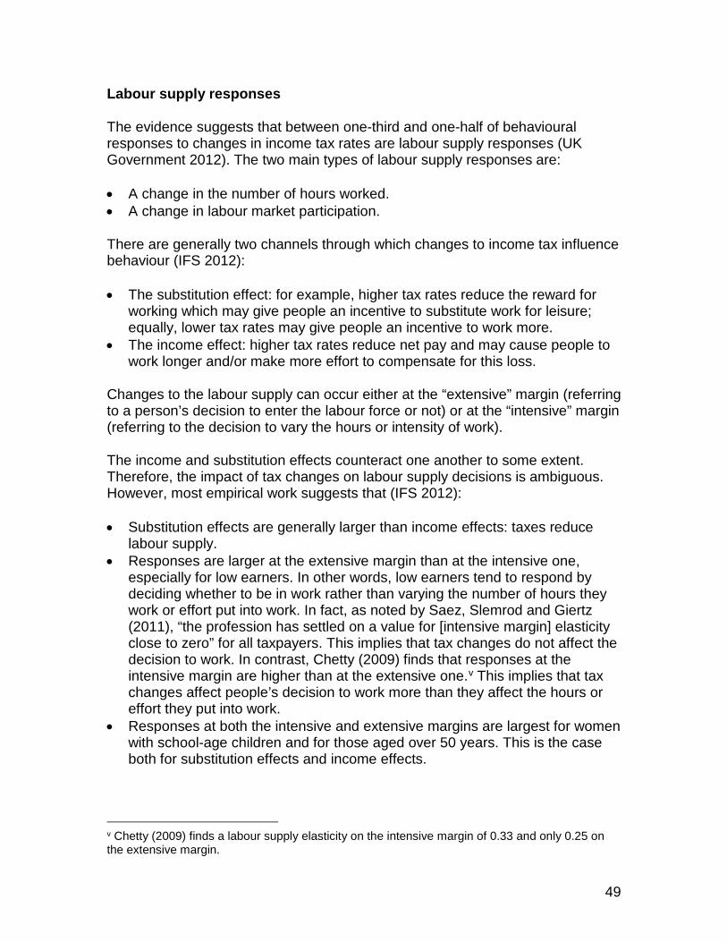
49

Labour supply responses

The evidence suggests that between one-third and one-half of behavioural responses to changes in income tax rates are labour supply responses (UK Government 2012). The two main types of labour supply responses are:

• A change in the number of hours worked. • A change in labour market participation.

There are generally two channels through which changes to income tax influence behaviour (IFS 2012):

• The substitution effect: for example, higher tax rates reduce the reward for working which may give people an incentive to substitute work for leisure; equally, lower tax rates may give people an incentive to work more.

• The income effect: higher tax rates reduce net pay and may cause people to work longer and/or make more effort to compensate for this loss.

Changes to the labour supply can occur either at the “extensive” margin (referring to a person’s decision to enter the labour force or not) or at the “intensive” margin (referring to the decision to vary the hours or intensity of work).

The income and substitution effects counteract one another to some extent. Therefore, the impact of tax changes on labour supply decisions is ambiguous. However, most empirical work suggests that (IFS 2012):

• Substitution effects are generally larger than income effects: taxes reduce labour supply.

• Responses are larger at the extensive margin than at the intensive one, especially for low earners. In other words, low earners tend to respond by deciding whether to be in work rather than varying the number of hours they work or effort put into work. In fact, as noted by Saez, Slemrod and Giertz (2011), “the profession has settled on a value for [intensive margin] elasticity close to zero” for all taxpayers. This implies that tax changes do not affect the decision to work. In contrast, Chetty (2009) finds that responses at the intensive margin are higher than at the extensive one.v This implies that tax changes affect people’s decision to work more than they affect the hours or effort they put into work.

• Responses at both the intensive and extensive margins are largest for women with school-age children and for those aged over 50 years. This is the case both for substitution effects and income effects.

v Chetty (2009) finds a labour supply elasticity on the intensive margin of 0.33 and only 0.25 on the extensive margin.

50

Labour market participation can change due to: • Migration (inward and outward); this is enhanced by open labour markets. • Retirement decisions. Emigration has the biggest impact on tax revenues as it leads to a permanent loss in income tax revenue but also other taxes (VAT, etc.). On the other hand, immigration can lead to a rise in tax revenue higher than expected without behavioural responses as the tax base grows. Retirement has an effect on income tax revenue and may have an effect on other taxes, but less so than migration. Changes in tax planning, avoidance and evasion These changes can be grouped into three categories: • An increase in tax planning or avoidance activities e.g. around tax relief,

converting income into capital gains, increasing contributions to private pensions, transferring income between spouses and entering into artificial avoidance schemes. These measures have a long-term effect on tax receipts and economic growth.

• An increase in evasion; this is a criminal act. This also has a long-term effect on taxes and growth.

• An increase in tax planning or avoidance activity, which has a one-off effect on tax liabilities. A common response if circumstances permit, is forestalling. This involves doing something in advance of a forthcoming change, for example:

- People may change the timing and/or nature of their income in anticipation of an income tax change.

- People may change the point at which they sell or buy a house in anticipation of a change in stamp duties.

Tax planning and avoidance are legitimate and are difficult to prevent using anti-avoidance measures. The UK Government circumvents this by announcing tax changes shortly before they come into effect. The vast literature on employment responses to hourly wage and other income changes highlights that the main avenue available for low income earners to respond to tax reform are labour supply responses, whereas medium to high income earners and the self-employed are more able to respond through tax planning and other additional avenues available to them (IFS 2012).

51

Migration The risk of migration may be increasing due to the increased labour mobility of highly skilled workers in the last 15 to 20 years as the legal impediments and general migration costs have reduced (UK Government 2012). For example, in a UK survey by the Skandia life assurance company in 2011, high taxation was the most frequently cited reason for considering leaving the UK (31% of respondents; UK Government 2012). The above study considered the extent to which people might consider leaving the UK and whether high taxation might influence this decision. There is limited empirical evidence on the extent to which high taxation played a role in the decision of emigrants to leave the UK. It is difficult to survey those who left the UK about the reasons for leaving the UK and whether high taxation influenced them. Indirect behavioural responses In addition to immediate effects on behaviour, taxes can have indirect, second-order, generally longer-term effects on behaviour. Firstly, some kinds of behavioural response will affect only income tax revenue whereas others will affect revenue from other taxes as well. A change in labour supply will generally have an impact on income tax revenue, as well as National Insurance contributions. This will impact on household spending as well, and so VAT revenues. Secondly, tax changes can have a long-term impact as people adapt to new circumstances. For instance, higher petrol taxes have more effect on petrol consumption in the long run as people seek more fuel-efficient cars and manufacturers respond by providing them (IFS 2012). Thirdly, tax rates may have an impact on economic growth. A cross-national study carried out by the OECD (2010) finds that this is the case, and that corporate taxes have the biggest impact, followed by income taxes, consumption taxes, and finally immovable property taxes. As noted by HMRC on the OECD’s study:

“This ranking reflects the way that each category of tax affects the decisions that firms and individuals make. These decisions determine the amount of labour that is supplied by households and demanded by firms, as well as the levels of saving, investment and the accumulation of human capital.” (UK Government 2012)

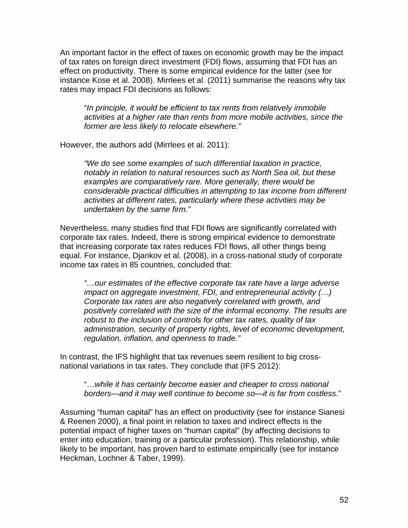
52

An important factor in the effect of taxes on economic growth may be the impact of tax rates on foreign direct investment (FDI) flows, assuming that FDI has an effect on productivity. There is some empirical evidence for the latter (see for instance Kose et al. 2008). Mirrlees et al. (2011) summarise the reasons why tax rates may impact FDI decisions as follows:

“In principle, it would be efficient to tax rents from relatively immobile activities at a higher rate than rents from more mobile activities, since the former are less likely to relocate elsewhere.”

However, the authors add (Mirrlees et al. 2011):

“We do see some examples of such differential taxation in practice, notably in relation to natural resources such as North Sea oil, but these examples are comparatively rare. More generally, there would be considerable practical difficulties in attempting to tax income from different activities at different rates, particularly where these activities may be undertaken by the same firm.”

Nevertheless, many studies find that FDI flows are significantly correlated with corporate tax rates. Indeed, there is strong empirical evidence to demonstrate that increasing corporate tax rates reduces FDI flows, all other things being equal. For instance, Djankov et al. (2008), in a cross-national study of corporate income tax rates in 85 countries, concluded that:

“…our estimates of the effective corporate tax rate have a large adverse impact on aggregate investment, FDI, and entrepreneurial activity (…) Corporate tax rates are also negatively correlated with growth, and positively correlated with the size of the informal economy. The results are robust to the inclusion of controls for other tax rates, quality of tax administration, security of property rights, level of economic development, regulation, inflation, and openness to trade.”

In contrast, the IFS highlight that tax revenues seem resilient to big cross-national variations in tax rates. They conclude that (IFS 2012):

“…while it has certainly become easier and cheaper to cross national borders—and it may well continue to become so—it is far from costless.”

Assuming “human capital” has an effect on productivity (see for instance Sianesi & Reenen 2000), a final point in relation to taxes and indirect effects is the potential impact of higher taxes on “human capital” (by affecting decisions to enter into education, training or a particular profession). This relationship, while likely to be important, has proven hard to estimate empirically (see for instance Heckman, Lochner & Taber, 1999).

53

Furthermore, some studies have found that personal income rates have a significant effect on entrepreneurial activity in the US (see for instance Gentry & Hubbard (2000) and Cullen and Gordon (2007). Effect on tax revenue Behavioural responses can lead to a permanent loss of tax revenue for the tax that has been changed but also for other taxes. For instance, if a taxpayer migrates, their income tax may drop to zero and they may reduce some if not all of their spending in the country of origin, which leads to a decrease in indirect taxes such as VAT. If an individual shifts their earnings into dividends, their liabilities for income tax on earnings decrease but their liabilities on dividend tax increase. This is discussed by Slemrod (1998) including the importance of accounting for shifts across tax bases (individual to corporate, for example) and across time (e.g., a shift to deferred compensation or greater use of retirement accounts). How are behavioural responses measured? Behavioural responses are measured using elasticity. This measures the change in the tax base (what is being taxed, for instance the price of a good for VAT, taxable income for income tax, property value for property taxes, etc.) after a tax change, due to behavioural responses. For income tax, this indicator is called taxable income elasticity (TIE). It measures the change in taxable income due to behavioural responses. For example, a TIE of 0.4 implies that a 1% change in the net-of-tax rate will lead to a fall in total taxable income of 0.4%. With TIEs, it is not necessary to separately measure all the underlying behaviours that influence taxable income and this became an increasingly popular way of assessing behavioural responses in the mid-1990s (Giertz 2010). TIE does not just take into account a change in the marginal rate of income tax. It looks at the change in the average rate of tax for a taxpayer – this includes all the tax rates they are liable for (e.g. basic and higher for higher rate taxpayers) as well as their National Insurance contributions. It is very difficult to measure behavioural responses and disentangle the effect of a tax change on taxpayers’ behaviour from other factors such as labour market conditions, inflation, etc. Various models have been developed over time to control for transitory and permanent shocks in income, leading to a wide range of methodologies and proposed elasticities which can be hard to compare: they use different measures of income for example, focus on different types of taxpayers, account for exogenous factors in different ways and use different statistical methods. In addition, as noted by Kopzcuk (2005), most studies fail to adequately isolate the effect of tax changes from other factors. The extent to which a tax change leads to behavioural responses is very difficult to estimate. Reasons for this include:

54

• Every tax change is different and it is likely that even if a given tax change is

identical to one in the past, other changes will also have occurred to the rest of the fiscal system.

• Economic circumstances may have changed leading to different incentives for taxpayers.

• Regulations (both national and international) may have changed, such as anti-avoidance measures.

Using empirical studies to predict future behavioural responses is problematic. Even two identical tax changes (for example, increasing the additional rate of income tax from 45p to 50p) will cause different behavioural responses. This is because two circumstances are never identical. There may have been: • Changes to the rest of the fiscal system. • Changes in the economy and aggregate shocks that cause varying income

trends which are hard to disentangle from tax-induced behavioural responses. • Changes to regulations such as anti-avoidance measures (different

opportunities for taxpayers). • Changes in composition of tax-paying population. • Differences in cultural factors when comparing different countries. When assessing the relevance of the conclusions they draw for the purposes of the present project, it is important to bear in mind that behavioural responses are highly idiosyncratic and depend on the economic situation, the nature of the tax system and the taxpayers who are affected at the time (culture, psychology, etc.). In addition, as mentioned, due to the absence of a counterfactual (“what would have happened if the tax had not been changed?”), it is challenging to disentangle the role of taxation, as opposed to other factors such as international trade and skill-based demand shocks (Gruber & Saez 2002). The following section provides a broad overview of the literature on this topic and explores ways in which behavioural responses could be included in EUROMOD. While the amount of evidence on the size of the TIE is growing, the IFS notes that it is still “rather limited” (IFS 2012). Most studies look at tax changes that have a direct impact on the individual; assessing the effect of changes to corporate and other taxation that does not impact directly on the individual is a very complex task (IFS 1994). Appendix 4 sets out empirical evidence on TIEs. Behavioural responses to benefit changes In order to assess the impact of changes to benefits and tax credits, we can explore changes in incentives individuals face to enter paid work or increase their earnings. Financial work incentives depend on the relationship between hours of

55

work and net income (after taxes and benefits), known as “budget constraint”. This depends on: • The amount of income received without working. • The gross wage rate an individual can command when working. • The taxes and benefits payable to or from them at different levels or earnings. The IFS (Browne, 2015) use summary measures of work incentives for modelling purposes. These are: • The incentive an individual faces to do paid work at all, as opposed to not

working; two measures are used to quantify a change in this incentive: - The participation tax rate (PTR), which measures the incentive to be in

paid work at all. It evaluates the proportion of gross wages that does not increase an employee’s net income because it is lost in either higher tax liabilities or lower benefit entitlements; this measures the extent to which the tax and benefit system distorts an individual’s decision whether to work or not.

- The replacement rate (RR), which evaluates the amount of income an individual receives when not working as a proportion of their in-work income. This measures the pure incentive to work people face.

• The incentive for someone already in work to earn a little more for instance by working more hours, seeking promotion or moving to a better-paid job. This is measured using the effective marginal tax rate (EMTR), the proportion of a small increase in earnings that is lost in either higher tax payments or lower benefit entitlements.

Higher RRs, PTRs and EMTRs all mean weaker work incentives. In Tax by Design, the IFS provide the distribution of PTRs and EMTRs among UK workers (Mirrlees et al. 2011). On PTRs, they state:

“PTRs are relatively low at low levels of earnings, on average, and especially for low-wage single parents and those with working partners, whose employment decisions are particularly responsive to financial incentives. The highest PTRs apply to sole earners in couples with children, and to a lesser extent to single people and sole earners in couples without children—the types of people who are likely to stay in work even if the incentive to do so is relatively weak.”

On EMTRs, the authors note:

“EMTRs are highest, on average, at an employer cost of about £170 a week, just before the peak of the earnings distribution: there are relatively few people at that point (who might reduce their incomes in response) but many people above that point (so the high EMTR delivers a lot of revenue). Average EMTRs are lower at, say, £400, around the peak of the

56

distribution. There are many people at that point (so strong disincentives would be damaging) and fewer people above it.”

Overall, they conclude:

“…high PTRs and EMTRs apply to people who stand to lose a lot of state support if they work—usually because they have children and/or substantial housing costs, and do not have a working partner whose earnings exhaust entitlement.”

The IFS (Browne, 2015) also provide a comprehensive methodology for analysing the effect of UK Government’s Spring 2015 Budget tax and benefit reform proposals. This methodology can in principle also be applied in the context of EUROMOD. However, it should be noted that (Browne, 2015):

“… changes in financial work incentive measures are only one element of what will determine what happens to employment levels over the next few years. First, although changes in work incentive measures will give us some sense of the direction and scale of likely changes in labour supply levels, these will ultimately also depend on how responsive people are to the changes in the incentives they face. Second, even if there are changes in the amount of labour individuals want to supply, this may or may not be matched by demand for this labour from employers.”

In addition, changes in work incentives have different effects on different people depending on their income levels, family circumstances, age, disability status, housing tenure and consumption patterns, partly because people’s tax liabilities and benefit entitlements depend on all these factors (Browne, 2015).

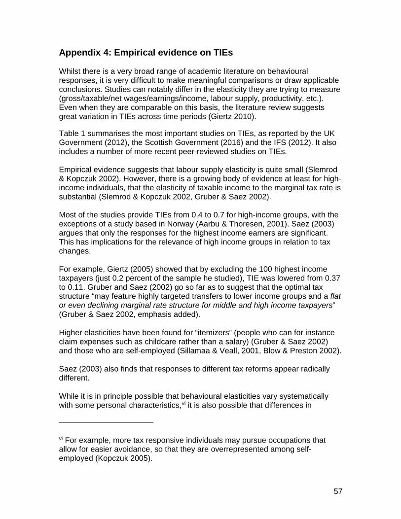
57

Appendix 4: Empirical evidence on TIEs Whilst there is a very broad range of academic literature on behavioural responses, it is very difficult to make meaningful comparisons or draw applicable conclusions. Studies can notably differ in the elasticity they are trying to measure (gross/taxable/net wages/earnings/income, labour supply, productivity, etc.). Even when they are comparable on this basis, the literature review suggests great variation in TIEs across time periods (Giertz 2010).

Table 1 summarises the most important studies on TIEs, as reported by the UK Government (2012), the Scottish Government (2016) and the IFS (2012). It also includes a number of more recent peer-reviewed studies on TIEs. Empirical evidence suggests that labour supply elasticity is quite small (Slemrod & Kopczuk 2002). However, there is a growing body of evidence at least for high-income individuals, that the elasticity of taxable income to the marginal tax rate is substantial (Slemrod & Kopczuk 2002, Gruber & Saez 2002). Most of the studies provide TIEs from 0.4 to 0.7 for high-income groups, with the exceptions of a study based in Norway (Aarbu & Thoresen, 2001). Saez (2003) argues that only the responses for the highest income earners are significant. This has implications for the relevance of high income groups in relation to tax changes. For example, Giertz (2005) showed that by excluding the 100 highest income taxpayers (just 0.2 percent of the sample he studied), TIE was lowered from 0.37 to 0.11. Gruber and Saez (2002) go so far as to suggest that the optimal tax structure “may feature highly targeted transfers to lower income groups and a flat or even declining marginal rate structure for middle and high income taxpayers” (Gruber & Saez 2002, emphasis added).

Higher elasticities have been found for “itemizers” (people who can for instance claim expenses such as childcare rather than a salary) (Gruber & Saez 2002) and those who are self-employed (Sillamaa & Veall, 2001, Blow & Preston 2002).

Saez (2003) also finds that responses to different tax reforms appear radically different.

While it is in principle possible that behavioural elasticities vary systematically with some personal characteristics,vi it is also possible that differences in

vi For example, more tax responsive individuals may pursue occupations that allow for easier avoidance, so that they are overrepresented among self-employed (Kopczuk 2005).

58

behaviour result from differences in the tax and institutional environment faced by different individuals (Kopczuk 2005).

Devereux (2004) shows there may be a negative and economically significant labour supply response of women to changes in their husband’s wages. This may partly explain why, as shown by Blundell and MaCurdy (1999), the responsiveness of male labour supply to after-tax wages is low, although it is higher (and perhaps much higher, namely if they have dependent children) for female/secondary earner labour supply. There have been few studies on the effect of tax changes in the UK on people’s behaviour. HMRC highlight that the most relevant study estimating a TIE for high incomes in the UK is the report by Brewer, Saez and Shephard (2008), which estimated a central TIE of 0.46 (UK Government 2012). Summary of key literature on TIEs Brulhart et al. (2016) Estimates of TIE

• percentage-point rise in wealth taxation lowers reported wealth by 3.5% in aggregate. Expressed relative to taxable capital income flows, this implies a net-of-tax elasticity of roughly 1.2 (this is large compared to literature)

• Elasticity of tax revenues with respect to tax rates -0.2 (implies that current rates are well below the revenue maximizing rate)

Comments • Switzerland (highest rate of annual wealth taxation in the developed world) • Study of wealth tax on reported wealth • Aggregate & micro data on wealth holdings by canton and individual-level

data for the canton of Bern. • Taxpayers bunch below the tax threshold (this is due to changes in

reported wealth and not by mobility) • Observed responses are driven by changes in wealth holdings rather than

mobility • Financial wealth is somewhat more responsive than non-financial wealth:

little distortion to wealth holdings from income taxation, but annual wealth tax has a considerable impact on wealth accumulation.

Saez (2016) Estimates of TIE

• Short-run TIE > 1 • 2011 to 2015: small medium-term response to tax increase • at most 20% of the projected tax revenue increase from the 2013 tax

reform is lost through behavioural responses. Comments

• US 2013 tax increase on top marginal tax rates on capital income by 9.5 points & on labour income by 6.5 points

59

• Uses tax statistics from the IRS • High short-run TIE due to income retiming for tax avoidance purposes and

is particularly high for realized capital gains and dividends, and highest at the very top of the income distribution.

• Conclusion: 2013 tax increase was an efficient way to raise revenue. Bell (2015) Estimates of TIE

• No estimates Comments

• Difficult to assess how findings from other studies can be applied in the Scottish context.

• Migration responses are potentially important. • Cultural acceptance of tax rate differences is probably country specific.

Milligan & Smart (2014) Estimates of TIE

• Elasticities of reported income are large for incomes in the top one percent, but small elsewhere.

Comments • Sub-national variation in Canadian provinces 1991 to 2010: look at income

reported by the top earners using the Canadian Tax and Credit Simulator to form tax rates & income data come from the CANSIM high income database (compares constructed income share data & real income data)

• Response happens both through earned and capital income UK Government (2012) Estimates of TIE

• Central estimate: 0.48 (“Monte Carlo simulation” estimates that true TIE for the model is likely to lie anywhere in the range of 0.14 to 0.81)

Comments • TIE within the range of academic studies and is close to the only other UK

study focusing on high income individuals Chetty et al. (2011) Estimates of TIE

• Lower bound of 0.34 (all income groups) Comments

• Denmark • Look at kink point in Danish tax data (where marginal rates jump) rather

than discrete tax changes Giertz (2010) Estimates of TIE

• Clear short-term behavioural response but not necessarily a longer-term response

60

• Incomes > $10,000 & with income controls TIE: 0 (single-year intervals) – 0.31 (three-year intervals)

• Incomes > $50,000 & with income controls TIE 0.19 (single-year intervals) – 0.33 (three-year intervals), hard to estimate over six-year period.

Comments • US 1990s tax increases (panel data for 1984, 1985 and 1988-1995) • Highlights that estimated elasticities when looking at US 1990s reforms

over a third smaller than analogous estimates for the 1980s • Controls for mean reversion • States: “it is incredibly difficult to isolate responses to changes in tax rates

from income changes due to myriad other complex factors.” Brewer et al. (2010) Estimates of TIE

• Top 1% of income earners: 0.46 (some as high as 0.7 without controls) Comments

• UK study: most relevant for estimating a TIE for high incomes in the UK • Assessment of effect of UK tax changes for top earners between 1978 &

2003 • Uses a difference-in-difference framework to compare the top 1% with

income groups just below this • Study does not explicitly control for diverging income trends • Summary:

o Second earners & low-education individuals have bigger extensive than intensive responses

o Responsiveness of hours worked may be as low as zero o Responsiveness of taxable earnings could be 0.25 for low-middle

income earners, rising for high-income earners o May be no scope for raising EMTRs for top earners in UK as this

may reduce government revenue • HMRC thinks TIE today might be higher than reported in this study as

labour mobility has increased over time, but also lower as the scope for tax avoidance is reduced

Chetty (2009) Estimates of TIE

• TIEs >0 and significant throughout the earnings distribution • Labour supply elasticity of 0.33 on the intensive margin & 0.25 on the

extensive margin Comments

• USA (Tax Reform Act 1986) • Theoretical paper (synthetic model)

Saez et al. (2009) Comments

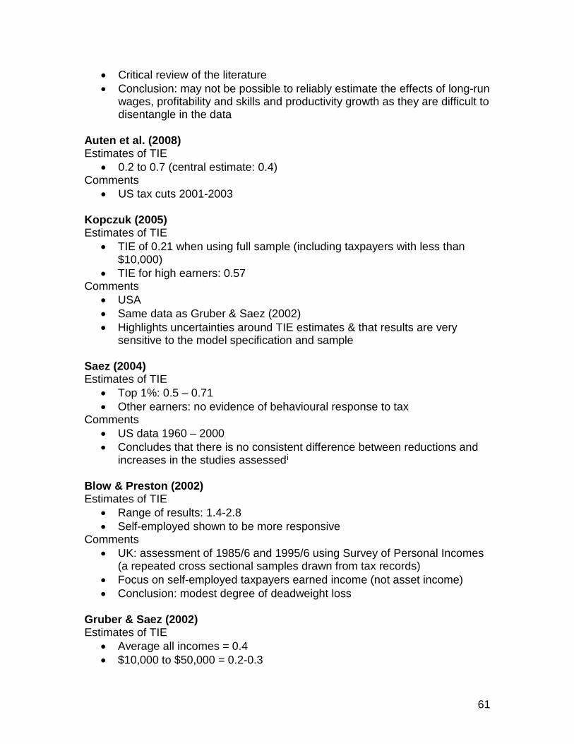
61

• Critical review of the literature • Conclusion: may not be possible to reliably estimate the effects of long-run

wages, profitability and skills and productivity growth as they are difficult to disentangle in the data

Auten et al. (2008) Estimates of TIE

• 0.2 to 0.7 (central estimate: 0.4) Comments

• US tax cuts 2001-2003 Kopczuk (2005) Estimates of TIE

• TIE of 0.21 when using full sample (including taxpayers with less than $10,000)

• TIE for high earners: 0.57 Comments

• USA • Same data as Gruber & Saez (2002) • Highlights uncertainties around TIE estimates & that results are very

sensitive to the model specification and sample Saez (2004) Estimates of TIE

• Top 1%: 0.5 – 0.71 • Other earners: no evidence of behavioural response to tax

Comments • US data 1960 – 2000 • Concludes that there is no consistent difference between reductions and

increases in the studies assessedi Blow & Preston (2002) Estimates of TIE

• Range of results: 1.4-2.8 • Self-employed shown to be more responsive

Comments • UK: assessment of 1985/6 and 1995/6 using Survey of Personal Incomes

(a repeated cross sectional samples drawn from tax records) • Focus on self-employed taxpayers earned income (not asset income) • Conclusion: modest degree of deadweight loss

Gruber & Saez (2002) Estimates of TIE

• Average all incomes = 0.4 • $10,000 to $50,000 = 0.2-0.3

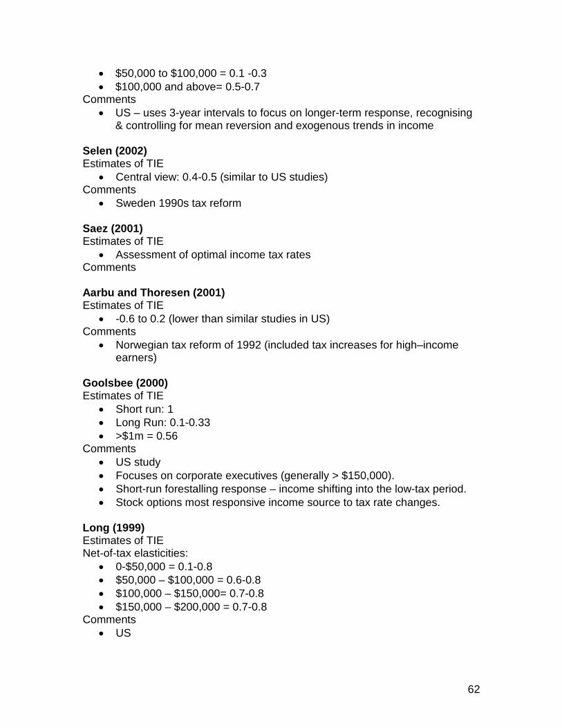
62

• $50,000 to $100,000 = 0.1 -0.3 • $100,000 and above= 0.5-0.7

Comments • US – uses 3-year intervals to focus on longer-term response, recognising

& controlling for mean reversion and exogenous trends in income Selen (2002) Estimates of TIE

• Central view: 0.4-0.5 (similar to US studies) Comments

• Sweden 1990s tax reform Saez (2001) Estimates of TIE

• Assessment of optimal income tax rates Comments Aarbu and Thoresen (2001) Estimates of TIE

• -0.6 to 0.2 (lower than similar studies in US) Comments

• Norwegian tax reform of 1992 (included tax increases for high–income earners)

Goolsbee (2000) Estimates of TIE

• Short run: 1 • Long Run: 0.1-0.33 • >$1m = 0.56

Comments • US study • Focuses on corporate executives (generally > $150,000). • Short-run forestalling response – income shifting into the low-tax period. • Stock options most responsive income source to tax rate changes.

Long (1999) Estimates of TIE Net-of-tax elasticities:

• 0-$50,000 = 0.1-0.8 • $50,000 – $100,000 = 0.6-0.8 • $100,000 – $150,000= 0.7-0.8 • $150,000 – $200,000 = 0.7-0.8

Comments • US

63

• High income taxpayers are found to be more responsive to rate changes than lower-income individuals, may be primarily due to access to reliefs and deductions.

Feldstein (1995) Estimates of TIE

• Central estimate 2.14, range 1 to 3 Comments

• US • Trend-setting study in the 1990s • May overestimate the impact of tax change

Blundell et al. (1998) Estimates of TIE

• Highlights that labour supply effects have been notoriously difficult to estimate in a robust and generally accepted way

• UK tax reforms in 1980s • Focus on labour supply responses of married or cohabiting women • Uses difference-in-difference method (provides a control group) • Positive & moderate wage elasticities • Negative income effects for women with children • Other income elasticities quite small and for women without children these

are zero Lindsey (1987) Estimates of TIE

• Central view 1.75, but as high as 2.75 Comments

• Trend-setting study in the 1980s – looks at income reported on tax returns • May overstate the TIE as does not control for income trends, so may

attribute rising income inequality to tax rate changes.

64

Appendix 5: Case study, 50p additional rate 2010-11 to 2013-14 In April 2010, the UK Government introduced a 50p rate of income tax for earnings above £150,000. The introduction of an additional rate of income tax at 50p was initially proposed in April 2009 (UK Government 2009). Table 2 shows the UK Government’s forecast revenue for the 50p rate between 2009 and 2010. Table 2: Forecast revenue raised at the 50p rate (and from 50% trust rate),

2010-11 to 2012-13, £m 2010-11 2011-12 2012-13 2009 Budget 1,130 1,810 n/a 2010 Budget 1,300 3,050 2,660

Source: UK Government 2009 & 2010

The UK Government used a TIE of 0.35 for its’ 2010 forecast. HMRC noted that this was deliberately at the low end of the academic elasticities surveyed (UK Government 2012). If there had been no behavioural response, the IFS estimated that the 50p rate would have raised £6.5bn in 2012-13 (Adam et al. 2012). This compares to the UK Government’s £2.7bn (Table 1). The IFS noted the Government had used a TIE of 0.35, which assumes quite a low behavioural response from affected taxpayers. The authors concluded (Adam et al. 2012):

“It is therefore clear that a substantial degree of behavioural response has been incorporated into [the UK Government’s] estimate.”

According to the IFS (Johnson & Phillips, 2014) “[perhaps] the best evidence” available on the TIE of the 50p rate is that produced by HMRC (UK Government 2012) in 2012 once all tax returns for 2010-11 had become available. HMRC note (UK Government 2012):

“The analysis shows that a considerable behavioural response to the rate change, including a substantial amount of forestalling: around £16 billion to £18 billion of income is estimated to have been brought forward to 2009-10 to avoid the introduction of the additional rate of tax (…). The modelling suggests the underlying behavioural response was greater than estimated previously in Budget 2009 and in March Budget 2010, decreasing the pre-behavioural yield by at least 83 per cent.”

It estimated TIEs of 0.40-0.48 for the introduction of the 50p rate, with a central measure of 0.45. In other words, the introduction of the 50p rate of income tax reduced taxable income by 0.45%. In his 2012 Budget speech in March 2012, the Chancellor George Osborne used HMRC’s estimate (UK Government 2012):

65

“HMRC finds that an astonishing £16 billion of income was deliberately shifted into the previous tax year, at a cost to the taxpayer of £1 billion—something that the previous Government’s figures made no allowance for whatsoever. Self-assessment receipts this year are below forecast by some £3.6 billion, while other tax receipts have held up. The increase from 40p to 50p raised just a third of the £3 billion that we were told it would raise.”

Although subject to a wide range of uncertainty, it estimated that forestalling may have increased 2009-10 liabilities by £7.3 billion, with a corresponding reduction in 2010-11 liabilities of £6.6 billion - the overall impact of forestalling on combined 2009-10 and 2010-11 liabilities therefore being around £0.7 billion (UK Government 2012). This is consistent with the £3.6 billion shortfall in Self-Assessment tax revenues observed in January and February 2012 (the months in which balancing payments relating to 2010-11 liabilities are received) (UK Government 2012). Forestalling of income other than dividends and employment income was relatively low (UK Government 2012). HMRC estimated that in 2010-11, 2011-12 and 2012-13, behavioural responses could have caused extra revenue to be two thirds lower than they otherwise would have been without a behavioural response. It estimated that in 2010-11 the 50p rate would raise £6.5 billion in income tax liabilities before behavioural responses were taken into account, but only £1.3 billion once they were included (UK Government 2012). The 50p rate may also have caused migration. In 2012, HMRC noted (UK Government 2012):

“The evidence on the impact of the 50 per cent rate on migration since its introduction in 2010 is more qualitative and anecdotal at this stage.”

This includes a 28% increase from the previous year in the number of British citizens working in the banking and financial services who moved to Switzerland in 2010 and a 29% increase in long-term work permits in 2010 (UK Government 2012). HMRC’s report also suggested that without any behavioural response, reducing the 50p rate to 45p could reduce revenues by about £3.5 billion in 2015-16. However, once behavioural responses were included, their central estimate was that revenue would only decrease by £100 million. This implies that raising the rate from 45p to 50p would also have raised around £100 million. The IFS commented on HMRC’s estimate and stated (Johnson & Phillips, 2014):

“…once one allows for behavioural response, their [HMRC’s] central estimate was a cost of just £100 million – a very small amount of money. The best available estimate of what reversing the cut would raise is therefore about £100 million too. However, it is important to bear in mind

66

that there is substantial uncertainty around this central estimate (…) HMRC’s central estimate is that this elasticity was 0.45 (…) If instead the true elasticity was 0.35 (which is well within the range of uncertainty), reducing the top rate of tax from 50p to 45p will have cost the exchequer about £700 million, whilst if the true elasticity was 0.55 (again, within the range of uncertainty), it will have actually raised about £600 million.”

The IFS concluded there was “little additional evidence to suggest that a 50p rate would raise more than was estimated by HMRC back in 2012” (Johnson & Phillips, 2014). This demonstrates the considerable uncertainty around estimates of behavioural responses. The Scottish Government (2016b) also highlighted the risk of behavioural responses on the Scottish budget when it published an analysis of the setting the 45p additional rate at 50p. It concluded (Scottish Government 2016b):

“There is therefore likely to be a significant revenue risk associated with increases to the Scottish additional rate of income tax above that applicable in the rest of the UK. A further risk will impact on future tax revenues where an increased additional rate of tax reduces the attractiveness of locating in Scotland in the future and reduces the potential economic and tax growth rates.”

When modelling the impact of income tax changes, HMRC modelling uses different TIEs for different income brackets defined in increments of £10,000, with higher TIEs for total income tax changes compared to tax changes in non-savings non-dividend (NSND) income. TIEs for total income tax range from 0 to 0.45 and TIEs for income NSND income range from 0 to 0.7.vii

vii Based on personal correspondence with HMRC.

67

Appendix 6: Estimating multiplier effects The Scottish Government publishes Input-Output tables each year. The tables provide an overview of the flows of goods and services in the Scottish economy for a given year and are available for the years 1998 to 2013 (the latest year available). The tables detail the relationship between producers and consumers and the linkages between different industries based in Scotland (Scottish Government, 2016a) One of the most significant interactions in Scotland’s economy is that between Scottish households and Scottish industries. Households sell labour to industry in exchange for income in the form of wages. Wages form a significant component of household income from which Scottish households purchase goods and services, partly produced by Scottish industries. The multiplier effect described above is set out in the Input-Output Methodology Guide published by the Scottish Government (2015). Type I multiplier effects capture the direct effects of an industry (including wages paid directly to industry employees). The type I multiplier also captures indirect effects stimulated through supply chain linkages where one Scottish industry purchases goods and services from another Scottish industry creating further jobs and income along the industry supply chain (Scottish Government, 2015). Estimating the flows of money in and out of households and the effect of these transactions upon industries is referred to as the induced effect. If the induced effect is added to the direct and indirect effects, it is referred to as a Type II multiplier. Put simply, households are treated as an additional industry by measuring the demand for labour from households through ‘compensation of employees’. The demand from households for goods and services produced by Scottish industries is measured through ‘household expenditure’. The last attempt, to the best of our knowledge, to disaggregate the household sector within a Scottish Input-Output model was undertaken by McNicoll and McLellan in 2003. Following the approach set out by McNicoll and McLellan an internal satellite extension was developed. The new data will act as a satellite to the existing Input-Output table (McNicoll, I. & McLellan, D, 2003). It is internal in that it is concerned with the disaggregation of data already contained in the tables rather than the addition of new data.

68

The Input-Output table usually contains a single column relating to household expenditure and a single row relating to household income. The single household row and column in the 2013 Scottish Input-Output tables were replaced with equivalent separate rows and columns for identified sub-sets of Scottish households in different income bands. This allowed the derivation of a "disaggregate Type II" Input-Output model for Scotland. The McNicoll and McLellan model was based on household income, this research used equivalised household income quartiles. This approach is preferable in order to categorise households based on their equivalised income drawing on data from the Living Costs and Food Survey (2013). Once households had been allocated to quartiles their aggregate unequivalised household income and spending was used to link the new household columns, reflecting household spending patterns, to the Input-Output table. The McNicoll and McLellan model also disaggregated the household row measuring income from employment from each industry. This helped to show what proportion of wages from each industry flowed to poorer or wealthier households. The household row was not disaggregated in the current model as the data available from the Living Costs and Food Survey (2013) was limited. The main influence on the household multiplier effect is the household spending column. Household expenditure was estimated based on total purchases of goods and services both domestically produced and imported. Import coefficients were then used to estimate the value of goods purchased and services produced within Scotland for each household income quartile. The McNicoll and McLellan model included household income quintiles and produced similar results. Income accruing to the lowest income quintile benefited the highest income quintile the most. Additionally, income accruing to the lowest income quintile had the highest overall impact on household income (across all quintiles). McNicoll and McLellan state their model “provides evidence both of "trickle up" (i.e. income receipts of the poorer benefiting the better-off) and "trickle down" (i.e. income receipts of the better-off benefiting the poorer)”. Similar trickle up and trickle down effects are evident in Scotland’s economy today as show in Table 5. Caution should be taken in interpreting the Input-Output model. The model is static and doesn’t consider marginal changes to consumption, the multiplier effects are fixed and will be the same for an additional £1,000 of household income or £10,000 of household income.

69

Appendix 7: Bridging results between income and deprivation The previous tax-benefit model used by III provided changes in equivalised household incomes by quintile resulting from changes in taxes and benefits. The III tool then mapped these changes directly to the 2016 Scottish Index of Multiple Deprivation (SIMD) in order to make a further estimate of changes in health outcomes. As EUROMOD is developed using the Family Resources Survey (FRS) it was possible to link the model with the 2013-14 FRS survey. This allowed the model’s tax-benefit variables to be matched to a wider range of indicators covering education, employment and health. The most recent SIMD includes the following domains, with % weights used by the Scottish Government for each domain shown in brackets; Income (28%), Employment (28%), Health (14%), Education, skills and training (14%), Geographic access to services (9%), Crime (5%) and Housing (2%). The indicators used to construct the income, employment, education and health domains are set out below: Income:

• Income Support and Income-based Employment Support Allowance claimants (16-59).

• Job Seekers Allowance and Guaranteed Pension Credit Claimants (All ages).

• Universal Credit claimants with no employment marker. • Number of children in JSA, IS or ESA households. • Number of adults and children dependent on adults in receipt of tax

credits.

Employment: • Unemployment Claimant Count averaged over 12 months. • Working age Incapacity Benefit or Employment Support Allowance

recipients. • Working age Severe Disablement Allowance Recipients.

Education:

• School pupil attendance. • School pupil performance. • Working age people with no qualifications. • 17-21 year olds enrolling into full time higher education. • School leavers aged 16-19 not in education, employment or training.

70

Health • Standardised Mortality Ratio. • Hospital stays related to alcohol misuse. • Hospital stays related to drug misuse. • Comparative Illness Factor. • Emergency stays in hospital. • Proportion of population being prescribed drugs for anxiety, depression or

psychosis. • Proportion of live singleton births of low birth weight.

Four indicators were chosen from the FRS:

• The proportion of those claiming Job Seekers Allowance (JSA) was used to represent the SIMD income domain.

• Whether any adults in the household were disabled under the Disability Discrimination Act (DDA) core definition was used to represent the health domain.

• Whether the household reference person held any qualifications was used to represent the education domain.

• The number who were unemployed (ILO definition) was used to represent the employment domain.

Each of the indicators was quantified by quintiles of three measures of household income: before housing costs (Table A2), after housing costs (Table A3) and equivalised household disposable income (Table A4). Each of the indicators was divided by the average to show the relative score of each quintile within each domain. The scores were multiplied by the weight for each domain to produce a weighted score for each quintile. The three different measures of household income reveal a similar pattern. The weighted deprivation score declines as household income rises. This suggests a direct mapping is likely between household income and the SIMD. However, the weighted score for quintiles 4 and 5 are similar suggesting there may be little difference in deprivation scores. The lowest household income quintile has by a sizeable margin the lowest weighted deprivation score.

71

Table A2: Weighted deprivation score by household income quintiles

(unequivalised before housing costs)

SIMD Weight 0.28 0.16 0.16 0.28 Weighted

Score Domain Income Health Education Employ

Quintile 1 4.0 1.3 1.5 5.4 3.0 Quintile 2 1.3 1.2 1.8 1.8 1.3 Quintile 3 0.6 1.2 1.1 0.8 0.7 Quintile 4 0.3 0.8 0.7 0.2 0.4 Quintile 5 0.1 0.6 0.4 0.3 0.3

Table A3: Weighted deprivation score by household income quintiles

(unequivalised after housing costs)




Table A4: Weighted deprivation score by equivalised disposable household

income




www.healthscotland.scot 6312

12/

2017

http://www.healthscotland.scot

Modelling the impact of policy interventions on income in ...

Documents

Transcript of Modelling the impact of policy interventions on income in ...