Lakes & Reservoirs: Research and Management

2002

7

: 189–199

Modelling the impact of historical land uses on surface-water quality using groundwater flow and

solute-transport models

Karen G. Wayland,

1

David W. Hyndman,

1*

David Boutt,

1

Bryan C. Pijanowski

2

and David T. Long

1

Departments of

1

Geological Sciences and

2

Zoology, Michigan State University, East Lansing, Michigan, USA

Abstract

Groundwater age, and its influence on contemporary water chemistry, needs to be accurately described to quantify thetemporally varying impacts of land use on water quality. The time lags between solute inputs at the land surface and impactson stream chemistry can be an important factor for managing land use in regional watersheds. Our approach uses a modifiedgroundwater flow code to simulate reverse groundwater flow, regional flow and the solute-transport model where a unitconcentration of a conservative solute serves as a proxy for groundwater age. Solute-contour lines represent groundwatertravel time, which can then be coupled with Geographic Information System analyses to examine the relationship betweenwater quality and historical land-use patterns. The reverse flow and solute modelling produced a reasonable distribution ofgroundwater travel times across the watershed, given the hydrology of the system. These groundwater flow paths would beunexpected if surface topography or even surface hydrology were used to predict groundwater movement. Approximately 70%of the watershed has a groundwater lag of

≤

30 years. When the temporal lags for individual drainage areas within the water-shed are compared, flush times vary dramatically. This variability is related both to the size of the sourceshed and its geology.The influence of a particular land use on stream chemistry changes depending on the time scale considered, and also depend-ing on the sourceshed in question as a result of landscape diversity. The results suggest that land-use management practicesto reduce solute loading to a watershed might not result in water-quality improvements for many years, especially if imple-mented on land far from streams. The influence of long groundwater flow paths that integrate past and current land uses mustbe considered in the interpretation of land-use effects on surface-water quality.

Key words

groundwater lag time, groundwater modelling, land use, water quality, watersheds.

INTRODUCTION

The biogeochemistry of surface water and groundwater arerelated to land use and land cover as well as to the geologyof a region. One of the most common approaches toexamine these relationships is to develop statistical correl-ations between water chemistry and current land use in thedrainage basins of surface-water sampling points. Althoughthis provides a good initial assessment, it does not accountfor the temporal lag for solutes to travel from the landsurface to discharge points at streams or lakes. This timelag is commonly a period of decades for the groundwater

inputs that supply the base-flow component of stream flow.Evaluating the distribution of time lags between the sourceinput and the impact on stream chemistry can be animportant factor for managing land use in regionalwatersheds.

The environmental impacts of land use/cover are notstatic in time or space. Variations in natural processes, suchas microbial activity or plant growth, or seasonal variationin land-use intensity can cause seasonal variations in streamchemistry. Temporal effects also occur on longer timescales. Recent research indicates that watershed land usein the 1950s was the best predictor of present-day aquaticinvertebrate and fish diversity in three North Carolinarivers (Harding

et al

. 1998). Surface-water quality samplestaken at low flow are known to be representative of thegroundwater chemistry in humid regions (Modica

et al

.

*Corresponding author.

Email: hyndman@msu.edu

Accepted for publication 24 June 2002.

190 K. G. Wayland

et al

.

1997). However, it is rarely considered that each stream-water sample taken at low flow represents a wide variety ofgroundwater ages, and thus reflects a time-weightedaverage of anthropogenic inputs from the land surface.Therefore, groundwater age, and its influence on contem-porary water chemistry, needs to be accurately describedto quantify the temporally varying impacts of land use onwater quality.

Ultimately, our research will explore whether a dynamicland-use database that incorporates temporal changes canbetter explain current stream chemistry than static data-bases of land use at a single point in time. This paperdescribes the first step of our work, which is the develop-ment of a groundwater flow and transport-modellingmethod that will allow us to link current stream chemistrymeasured at base flow with historical land-use distri-butions. Groundwater age distributions will be coupledwith Geographic Information System (GIS)-derived land-use patterns to improve our understanding of the time lagbetween watershed-scale landscape changes and observedeffects in surface waters. The approach presented in thiswork provides critical input for watershed planners on thepotential delay between implementing land-use manage-

ment strategies and observing improvements in surface-water quality.

STUDY SITE

The Grand Traverse Bay Watershed (GTBW) in theNorthern

Lower

Peninsula

of

Michigan

(Fig. 1)

waschosen for this research because of the rapid populationgrowth

and

land-use

intensification

occurring

in

theregion over the past several decades. The region was arelatively

pristine

watershed

and

has

had

increasedurban

and

agricultural

development

over

the

past50 years.

As

a

result,

there

is

increased

concern

aboutthe impacts of these

changes

on

the

high-quality

surfaceand

groundwater resources. Grand Traverse Bay is one ofthe last remaining oligotrophic bays in Lake Michigan.However, a 1998 summary of conditions in the bayindicated that the water quality in near-shore areas hasdeteriorated as a result of nutrient loading (Grand TraverseBay Watershed Initiative 1998). Previous work in thewatershed

has

documented

potential

correlationsbetween

high

nitrate

concentrations

in

groundwaterand

cherry

orchards

(Rajagopal

1978).

Nitrogen

loadingin the watershed

has

also

been

linked

to

atmospheric

Fig. 1. Grand Traverse Bay

Watershed, Michigan.

Land use legacy effect on water quality 191

deposition, animal waste, septic tanks and fertilizers(Cummings

et al

. 1990).The 2600-km

2

watershed contains over 100 lakes,including the Torch and Elk Lakes systems. The BoardmanRiver is the main tributary draining the GTBW and exertsa strong influence on groundwater flow and gradient in thesouthern half of the watershed (Cummings

et al

. 1990;Boutt

et al

. 2001). The surficial sediments of the watershed,which can be as thick as 275 m, are predominantly glacialoutwash, till, lacustrine sand and gravel, and dunes, all ofwhich overlay shale and limestone bedrock (Cummings

et al

. 1990; Boutt

et al

. 2001). The water table is close to thesurface in most areas of the watershed. Drinking-waterwells

in

the

area

are

generally

screened

in

the

range

of15–45 m below ground surface in the outwash and lacus-trine deposits (Cummings

et al

. 1990). The water tablefluctuates seasonally, with highest levels in the winter andspring, and lowest levels in the summer (Cummings

et al

.1990).

Land use/land cover in the watershed is predominantlyforest (49%) and agriculture (20%; Fig. 2). Urban land usecomprises 6% of the total area of the watershed, with theTraverse City urban region located on the shores of GrandTraverse Bay. The other main land cover categories areshrub/brush (15%), water (9%) and wetlands (1%). Land-use distributions for our analysis were obtained from the1980 Michigan Resource Inventory System database(MIRIS). The population of the greater Grand Traverse Bayregion has increased by 42% from 1980 to 2000, resulting in

greater intensification of the 1980 land uses rather than insignificant changes in land-use distributions. This is largelya result of the fact that almost all the forested land in thewatershed is protected state forest and thus cannot beconverted to any other land use.

The work described in this paper is part of a largerresearch effort in the GTBW to study the relationshipbetween land use and water-quality indicators. Othercomponents of this project include the development ofgeochemical fingerprints of land use through synopticsampling of approximately 80 surface water-sampling sitesin the watershed, modelling land-use change based onsocioeconomic drivers, and fingerprinting

Escherichia coli

deoxyribonucleic acid to identify bacterial sources tostreams and beaches. We previously developed andcalibrated a groundwater-flow model for this region andsimulated the transport of chloride from road salt to surfacewater-bodies (Boutt

et al

. 2001). This model showed thatalthough road salt is not the only source of chloride to thiswatershed, it is does appear to be the most significant on aregional scale. Through our surface-water samplingprogramme, we have also found strong associationsbetween the amount of urban land in a drainage area andelevated levels of sodium, potassium and chloride instreams (Wayland

et al

. 2003).

METHODSGrand Traverse Bay Watershed flow model

The groundwater model that was used in this research hastwo layers, over one million grid 100

×

100 m cells, andmore than 34 000 river cells (Boutt

et al

. 2001). Aquiferproperties were obtained by compiling records of oil andgas wells and residential drinking wells in the watershedalong with information from a detailed map of surficialgeology (Farrand & Bell 1982). The shale formation under-lying the surficial aquifer or the overlying thick clay layerpresent in some areas of the watershed was identified inregional well logs and geostatistically interpolated to pro-vide the bottom of the simulated aquifer. This shale/clayunit is assumed to be a confining layer impeding verticalflow. Six zones of similar glacial units were identified andassigned unique hydraulic conductivity values based onpump tests (Cummings

et al

. 1990) or published values forsimilar materials (Freeze & Cherry 1979). Both layers wereassigned the same value except where lacustrine sand andgravel overlied low conductivity clays. Head distributionssimulated by the flow model accurately representedobserved heads across the watershed; thus, the model wasused to produce the reverse vectors necessary to simulategroundwater age distributions.

Fig. 2.

Distribution of urban, agriculture and forested land in the

Grand Traverse Bay Watershed.

192 K. G. Wayland

et al

.

The hydrologic boundary of the groundwater system isshown in Fig. 3 overlain by the watershed boundary asdetermined by surface topography. The surface boundaryis typically used to delineate the area of watershed formanagement purposes, but groundwater inputs to thecorresponding

surface

water-body

might

not

coincidewith areas generating overland flow. Subwatersheds, orsourcesheds, also have different boundaries when deter-mined by surface topography and groundwater flow.

Reverse groundwater flow modelling approach

Direct methods for dating groundwater age, such as iso-topes and environmental tracers, rely on decay constants(isotopes) or time of introduction into the environment(environmental tracers such as chlorofluorocarbons andtritium). These methods are primarily useful for deter-mining recent groundwater from older water (Domenico &Schwartz 1990). Direct methods cannot delineate specificareas within a sourceshed that have contributed ground-water to a stream over a specific time period due tolimitations

caused

by the mixing of waters of differentages and the uncertainty of production, deposition anddecay. Groundwater age distributions can be developedusing a relatively new modelling technique introduced byGoode (1996). Goode’s direct simulation method uses amodified solute-transport equation with age substituted forconcentration and a unit ageing term that increases by onefor each day of the simulation (Goode 1996; Varni &Carrera 1998). An alternative modelling technique thathas received little attention in the literature is reverse-flow modelling, which was used in this project togenerate groundwater age distributions for eachsourceshed.

Our approach involved modifying the regional flow andsolute-transport model to simulate reverse groundwaterflow, the resulting flow distributions at each time step arecoupled with GIS analysis to examine the relationshipbetween water quality measured at surface-water samplingsites and historical land-use patterns in each sampling site’sdrainage area. We first estimated the source region of waterto each stream reach between sampling points, which wecalled a ‘sourceshed.’ The development of sourcesheds willbe explained in greater depth below. We then simulated thetravel time for water to reach the stream by trackingparticles backwards from the streams to the water tablealong simulated groundwater flow paths. This groundwatertransport time map depicted the time for groundwater toflow to reach any surface water-body, which ranges fromcurrent ages near streams to decades-old ages far fromstreams.

The regional flow and solute-transport model (Bouttet al. 2001) was used to simulate groundwater flow movingaway from perennial streams instead of flowing to thesedischarge points. A similar approach was used to estimatehistorical nitrogen loading from the Waquoit Bay water-shed (Brawley et al. 2000). Brawley et al. (2000) usedreverse-particle tracking to establish flow paths andgroundwater travel times from streams, bay shoreline andponds. Our approach differed in two respects. First, reverseflow is achieved by modifications to the MODFLOW codeso that water flowed from surface-water discharge pointsbackwards to recharge points. Forward-flow vectors weremultiplied by −1 to produce reverse-flow vectors, and therecharge flux became evapotranspiration loss. Second, thesolute-transport modelling with the MT3D code producedadvective fronts that represented contour lines of traveltime. Rather than tracking specific particles to establishtravel times as was done by Brawley et al. (2000), allsurface water-bodies became sources of an unreactivespecies with a constant concentration of 1. As the solute-transport simulation progressed, a concentration frontmoved from discharge to recharge along groundwater

Fig. 3. Groundwater and surface-water boundaries for the Grand

Traverse Bay Watershed and sourcesheds.

Surface water sampling siteGTBW surface water boundarySourceshed surface water boundarySourceshed groundwater boundaryGTBW groundwater boundary

Land use legacy effect on water quality 193

flow paths. Areas within the concentration front wereexpected to contribute recharge water to surface water-bodies over the specified time-frame.

The model was run for 150 years and output was saved atannual time-steps. Output files for annual time-steps wereprocessed by converting all cells with concentrations>0.5–1 and concentrations <0.5 as 0 because the advectivefront was represented by the 50% arrival location inadvection dispersion simulations. All processed outputfiles were then summed together to provide the number ofyears that an advective front was present. The final ground-water legacy map was then produced by subtracting thissum by one less than the maximum number of years (149).For ease of data manipulation, cell information was aggre-gated into 10-year intervals. This groundwater transport-time database depicts the time for groundwater to flow toreach any surface wate- body, which will range fromcurrent ages near streams to decades-old ages far fromstreams.

SourceshedsThe resulting flow distributions at each time step arecoupled with GIS analysis to examine the relationshipbetween water quality and historical land-use patterns.We have developed both groundwater and surface-watersourcesheds for each sample point. Surface-watersourcesheds are based on digital elevation models (DEM)data, and groundwater sourcesheds were developed fromthe groundwater model. Although development of agroundwater flow model is the most accurate method ofdetermining groundwater sourcesheds, they can also bedeveloped using an interpolated map of measured headdata, provided that enough data are available to approxi-mate the location of the water table. Thus, an assessment ofregional land-use impacts on stream-water quality can bedeveloped without the expense of model development.

Sourcesheds were created by converting the DEM datainto ground contour lines using the WATERSHED com-mand in the GRID module of the Arc/Info geographicinformation system (ESRI, Redlands, CA, USA). A rasterdrainage network was generated in GRID using theFLOWDIRECTION and FLOWACCUMULATION com-mands in Arc/Info GRID. Each sampling point was thenassigned to a grid cell within the drainage network. TheWATERSHED process requires a set of one or more seedpoints for which a drainage area will be delineated. Todelineate the total sourcesheds, an Arc Macro Languagescript was used to iteratively select the 80 sample sites andseed the DEM using only one site at a time. Followingdelineation, each set of sourcesheds was converted topolygons. The polygon layer was then intersected with a

gridded Level 1 Anderson land use/land cover data fromthe 1980 MIRIS.

The travel-time contour files for each decadal intervalwere clipped with the boundaries of each groundwatersourceshed using Arc/INFO. Data were organized byan integer code (001–147) containing information aboutdecade and land use. Each line of data was assigned a coderepresenting the decade (0–14) and the appropriateAnderson Level I land-se category (1–7) from the MIRISdatabase. For example, the value 21 represents the period20–30 years before present and the land-use categoryurban (1). The value 103 indicates years 100–110 beforepresent and forested land (3). The resulting grids werethen stored as individual raster grids for future analysis.The portion of each sourceshed polygon in a particular landuse for each decade was calculated by summing cells in thatland use. The 3-digit combined code was then separatedback into two sets of codes representing decade and landuse. The resulting table was exported to a spreadsheetprogram and used to examine changes in the contributingarea of a sourceshed over time, and also how land-usedistributions within contributing area changes with decade.

SURFACE-WATER SAMPLINGThe sourcesheds discussed in the following section werechosen based on a comparison of estimated annual massloadings of nitrate, sodium and chloride at different sites inthe watershed. Surface-water samples and flow measure-ments were taken during base-flow synoptic sampling inOctober 2000 at approximately 63 sites within the water-shed. Sites 2, 5, 9 and 12 consistently had some of thehighest mass loadings of solutes (Fig. 3). These sites werealso located in different regions of the watershed, andcurrently have a wide range of land-use types. Sites 2, 5 and9 are mixed-use sourcesheds undergoing rapid urbaniz-ation, particularly in the downstream regions near theGTBW shore. Site 12 is located at the mouth of the southbranch of the Boardman River and drains forested andagricultural land. In a typical watershed planning scenario,these drainage areas would receive high priority formanagement activities because of their contributions tototal pollutant loads from the watershed, and we thereforechose to illustrate the relationship between land use andgroundwater age in these four sourcesheds.

RESULTS AND DISCUSSIONGroundwater flow and age distribution

The reverse flow and solute modelling produced a distri-bution of groundwater travel times across the watershedthat appears to be reasonable given the hydrology of the

194 K. G. Wayland et al.

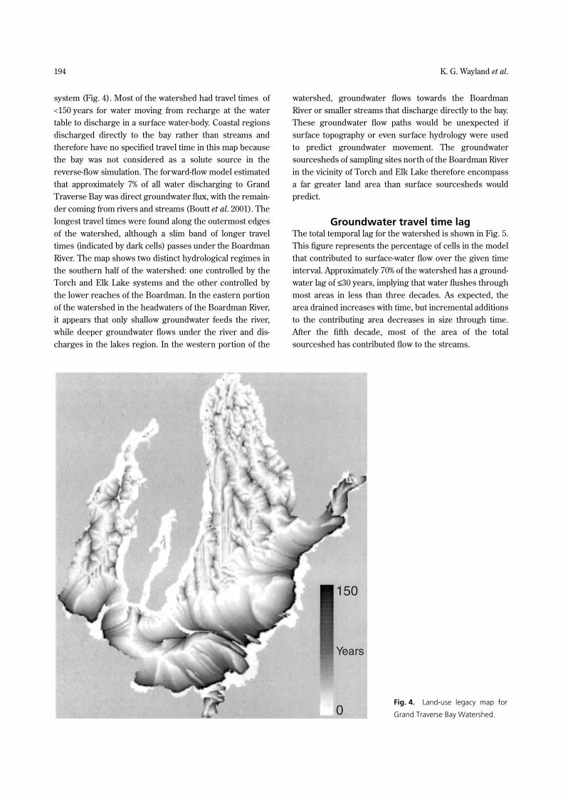
system (Fig. 4). Most of the watershed had travel times of<150 years for water moving from recharge at the watertable to discharge in a surface water-body. Coastal regionsdischarged directly to the bay rather than streams andtherefore have no specified travel time in this map becausethe bay was not considered as a solute source in thereverse-flow simulation. The forward-flow model estimatedthat approximately 7% of all water discharging to GrandTraverse Bay was direct groundwater flux, with the remain-der coming from rivers and streams (Boutt et al. 2001). Thelongest travel times were found along the outermost edgesof the watershed, although a slim band of longer traveltimes (indicated by dark cells) passes under the BoardmanRiver. The map shows two distinct hydrological regimes inthe southern half of the watershed: one controlled by theTorch and Elk Lake systems and the other controlled bythe lower reaches of the Boardman. In the eastern portionof the watershed in the headwaters of the Boardman River,it appears that only shallow groundwater feeds the river,while deeper groundwater flows under the river and dis-charges in the lakes region. In the western portion of the

watershed, groundwater flows towards the BoardmanRiver or smaller streams that discharge directly to the bay.These groundwater flow paths would be unexpected ifsurface topography or even surface hydrology were usedto predict groundwater movement. The groundwatersourcesheds of sampling sites north of the Boardman Riverin the vicinity of Torch and Elk Lake therefore encompassa far greater land area than surface sourcesheds wouldpredict.

Groundwater travel time lagThe total temporal lag for the watershed is shown in Fig. 5.This figure represents the percentage of cells in the modelthat contributed to surface-water flow over the given timeinterval. Approximately 70% of the watershed has a ground-water lag of ≤30 years, implying that water flushes throughmost areas in less than three decades. As expected, thearea drained increases with time, but incremental additionsto the contributing area decreases in size through time.After the fifth decade, most of the area of the totalsourceshed has contributed flow to the streams.

Fig. 4. Land-use legacy map for

Grand Traverse Bay Watershed.

Land use legacy effect on water quality 195

When the temporal lags for individual sourcesheds arecompared, flush times vary dramatically. Figure 6 showsthe cumulative proportion of the total sourceshed area thatcontributes to current stream water in a given decade andthe incremental area added during each decade. While 70%of the Site 2 sourceshed area has a groundwater lag of lessthan 30 years, at Site 5 the lag time is closer to 80 years.Sites 9 and 12 have 70% lag times of 7 decades. Water movesfrom the farthest reaches of the sourceshed to the outletin 70, 120, 140 and 120 years for Sites 2, 5, 9 and 12,respectively, based on 95% of the total area of eachsourceshed.

Variability in flush times is related both to the size ofthe sourceshed and its geology. Site 2 is the smallestsourceshed with an area of approximately 18 km2; sites 5,9, and 12 are 95, 110 and 212 km2, respectively. The effectsof geology are reflected in the incremental additions ofarea, as shown in Fig. 6, and also in the change of the slopein the cumulative area curves. The slopes of the curves

are shallower as water moves through areas of lowerhydraulic conductivity, such as tills (3 m/day) and dunesands (10 m/day). Water moves faster through lacustrinesand and gravel deposits (21 m/day) and outwash plains(24 m/day) and, therefore, more area per decade is addedto the contributing area of the sourceshed in higherconductivity zones. The best example of this effect can beseen at Site 5 where the cumulative percent curve showspronounced steps as the geology changes from sandand gravel to end moraine to outwash moving from themouth of the sourceshed to its headwaters. The bottomcurve representing the incremental addition of area perdecade has two peaks during which a greater percentageof area is added to the sourceshed. These peaks likelycorrespond to high conductivity zones within thesourceshed.

There are several implications of differences in flushtimes across a watershed for land-use planners and environ-mental managers. The reverse-flow model shows that thetime period for groundwater to move through 90% of thearea of a sourceshed fluctuates spatially in the GTBW(Fig. 7). The shortest flush times (20–50 years) occur insmall coastal sourcesheds, while larger coastal source-sheds and the downstream reaches of large streams canhave 90% flush times exceeding 80 years. Watershed-management strategies applied uniformly across the land-scape to reduce solute loading will therefore have variableinfluence on stream chemistry related to the flush time ofindividual sourcesheds. An understanding of flush-timedistributions can help target priority drainage areas andalso create realistic expectations for the short-termeffectiveness of management activities.

Fig. 5. Proportion of total watershed flushed at a given time

interval.

Fig. 6. Variations in flush times and incremental area/decade for individual sourcesheds. (–�–) Cumulative area (%), (�) total area (%).

196 K. G. Wayland et al.

A second and related implication of our results is thatregardless of the size or geology of a sourceshed, the lagtime between groundwater recharge at the landscapesurface and discharge in surface waters is significantlylonger than the life of most management plans. Land-useplans are typically developed for relatively short timeperiods compared to groundwater travel times. Countymaster plans in Michigan are redrawn at 5-year intervals;state environmental grants rarely exceed the same timeperiod. Therefore, 20 years might be considered long-termplanning. The effects of management practices might notresult in water-quality improvements for many years,especially if implemented on land far from streams. In theGTBW, 60–80% of many smaller sourcesheds are drained in20 years, while in some of the large sourcesheds, ground-water moves through less than 20% of the area duringthe same time period (Fig. 8). Furthermore, managementstrategies to improve surface-water quality frequently focuson infiltration enhancement to reduce overland flowbecause run-off is often the greatest source of non-pointsource pollution in a watershed. Cassell & Clausen (1993)modelled a shift in phosphorus export from a field after

run-off controls were implemented to increased loadingthrough infiltration. Thus, some management strategiesmight initially improve water quality while resulting incontinued loading to the groundwater system that willeventually discharge to surface waters. This is particularlya concern for conservative species, such as chloride and, tolesser extent, sodium.

Changing influence of land use on stream chemistry

Land uses are not evenly spread across landscapes and,therefore, the land-use distribution in the contributing areaof a sourceshed will change as travel time front movesthrough the sourceshed. The patchiness of landscapes isreflected in Fig. 9. Each curve represents the cumulativetotal of a land use within the contributing area for the timestep divided by the total sourceshed area. In other words,the influence of a particular land use on stream chemistrychanges depending on the time scale considered, and alsodepending upon the sourceshed in question as a result oflandscape diversity. Site 2 does not exhibit much landscapediversity while Site 5 has patches of different land uses that

Fig. 7. Flush time for 90% of

total sourceshed area.

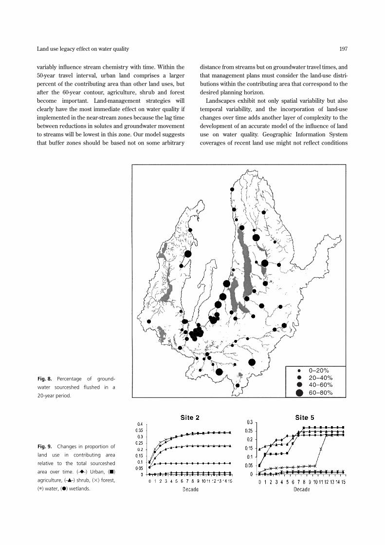
Land use legacy effect on water quality 197

variably influence stream chemistry with time. Within the50-year travel interval, urban land comprises a largerpercent of the contributing area than other land uses, butafter the 60-year contour, agriculture, shrub and forestbecome important. Land-management strategies willclearly have the most immediate effect on water quality ifimplemented in the near-stream zones because the lag timebetween reductions in solutes and groundwater movementto streams will be lowest in this zone. Our model suggeststhat buffer zones should be based not on some arbitrary

distance from streams but on groundwater travel times, andthat management plans must consider the land-use distri-butions within the contributing area that correspond to thedesired planning horizon.

Landscapes exhibit not only spatial variability but alsotemporal variability, and the incorporation of land-usechanges over time adds another layer of complexity to thedevelopment of an accurate model of the influence of landuse on water quality. Geographic Information Systemcoverages of recent land use might not reflect conditions

Fig. 8. Percentage of ground-

water sourceshed flushed in a

20-year period.

Fig. 9. Changes in proportion of

land use in contributing area

relative to the total sourceshed

area over time. (–�–) Urban, (�)

agriculture, (–�–) shrub, (�) forest,

(�) water, (�) wetlands.

198 K. G. Wayland et al.

in the watershed during most of the transport period.More robust chemical signatures for individual land usesmight appear if the legacy of land use is consideredinstead of a static distribution of land uses based on asingle year, as is shown in Fig. 9. The next step in ourresearch is to merge the areas for each decadal time stepwith a land-use database corresponding to the appropriatetime interval.

CONCLUSIONSThe approach presented in this paper provides a ground-water transport-time distribution that can be coupled withGIS-based land-use data to improve our understanding oflinkages between land use and surface-water chemistry. Werecognize that the impacts of overland flow and near-surface groundwater flow during storm events representsa significant source of anthropogenic solutes to a water-shed. However, our approach addresses the impact of landuse on stream chemistry through groundwater inputs, bothspatially and temporally, which is rarely given weight inmanagement plans. The results from preliminary workwith this approach illustrate the importance of consideringthe time lag between management activities in uplandregions and effects in surface waters. Regions that haverapid transport to surface water can be quickly identified onthe map of predicted travel times. Thus, rather thandeveloping stream buffer zones based on some arbitrarydistance, they can be determined based on the simulatedtravel time to surface water-bodies. The groundwater-flowmodel also emphasizes that surface topography does notalways coincide with groundwater-flow patterns and, there-fore, groundwater sourcesheds should be delineated alongwith surface sourcesheds to accurately target land usescontributing solutes to streams. In addition, the degree towhich constituents measured in surface-water samplesactually arise from groundwater inputs, and the influenceof long groundwater-flow paths that integrate past withcurrent land uses must be considered in the interpretationof land-use effects on surface-water quality.

Groundwater-travel time from recharge to discharge canbe ≥100 years in some watersheds and, therefore, base flowis a mixture of groundwater ages. Therefore, base-lowgeochemistry is an integration of land use, both spatiallyand temporally. Effective watershed modelling andmanagement efforts must address the imprint of pastland uses on groundwater, or the land-use legacy. Morerobust relationships between stream chemistry and landuses might appear if a dynamic database of land uses isconsidered instead of a static distribution of land usesbased on a single year. Future work with the reversegroundwater flow and solute-transport model will include

the incorporation of multiple databases on land-use distri-butions in the watershed as far back as 1938. The model willalso be used to predict the sensitivity of water quality atindividual sampling sites to different land uses.

REFERENCESBoutt D. F., Hyndman D. W., Pijanowski B. P. & Long D. T.

(2001) Modeling impacts of land use on groundwaterand surface water quality. Ground Water 39, 24–34.

Brawley J. W., Collins G., Kremer J. N. & Sham C. H.(2000) A time-dependent model of nitrogen loading toestuaries from coastal watersheds. J. Environ. Qual. 29,1448–61.

Cassell E. A. & Clausen J. C. (1993) Dynamic simulationmodeling for evaluating water quality response to agri-cultural BMP implementation. Water Sci. Technol. 28,635–648.

Cummings T. R., Gillespie J. L. & Grannemann N. G.(1990) Hydrology and land use in Grand TraverseCounty, Michigan. US Geological Survey, Open FileReports Section, Denver, CO; 90–4122.

Domenico P. & Schwartz F. W. (1990) Physical andChemical Hydrogeology. John Wiley and Sons, NewYork.

Farrand W. & Bell D. (1982) Quaternary Geology ofSouthern Michigan. University of Michigan. Ann ArborMI.

Freeze R. A. & Cherry J. A. (1979) Groundwater. PrenticeHall, Englewood Cliffs, N.J.

Goode D. J. (1996) Direct simulation of groundwater age.Water Resources Res. 32, 289–96.

Grand Traverse Bay Watershed Initiative. (1998) GrandTraverse Bay: State of the Bay. Grand Traverse BayWatershed Initiative, Traverse City, Michigan.

Harding J. S., Benfield E. F., Bolstad P. V., Helfman G. S. &Jones E. B. (1998) Stream biodiversity: the ghost of landuse past. Proc. Natl. Acad. Sci. 95, 14 843–7.

Modica E., Reilly T. E. & Pollock D. W. (1997) Patterns andage distribution of ground-water flow to streams.Ground Water 35, 523–37.

Rajagopal R. (1978) Impact of land use on ground waterquality in the Grand Traverse Bay region of Michigan.J. Environ. Qual. 7, 93–8.

Varni M. & Carrera J. (1998) Simulation of groundwaterage distributions. Wat. Resources Res. 34, 3271–81.

Wayland K. G., Long D. T., Hyndman D. W., Pijanowski B.& Woodhams S. M. (2000) Biogeochemical fingerprint-ing of a rapidly urbanizing watershed. In: Proceedings ofthe 8th National Nonpoint Source Monitoring Workshop(ed. J. C. Clausen). Environmental Protection Agency,Chicago, IL; EPA/905–R–01–008.

Land use legacy effect on water quality 199

Wayland K. G., Long D. T., Hyndman D. W., PijanowskiB. C., Woodhams S. M. & Haack S. K. (2003) Identifyingrelationships between baseflow geochemistry and land

use with synoptic sampling and R–mode factor analysis.J. Environ. Quality. (in press)