Modelling the High-Frequency FX Market: An Agent...
183
Modelling the High-Frequency FX Market: An Agent-Based Approach Monira Essa Aloud A thesis submitted for the degree of Doctor of Philosophy School of Computer Science and Electronic Engineering University of Essex April 2013
Transcript of Modelling the High-Frequency FX Market: An Agent...

Modelling the High-Frequency FX Market: AnAgent-Based Approach
Monira Essa Aloud
A thesis submitted for the degree ofDoctor of Philosophy
School of Computer Science and Electronic EngineeringUniversity of Essex
April 2013

i
Abstract
In this thesis, we use an agent-based modelling (ABM) approach to model the trad-
ing activity in the Foreign Exchange (FX) market which is the most liquid financial
market in the world. We first establish the statistical properties (stylized facts) of the
trading activity in the FX market using a unique high-frequency dataset of anonymised
individual traders’ historical transactions on an account level, spanning 2.25 years. To
the best of our knowledge, this dataset is the biggest available high-frequency dataset
of individual FX market traders’ historical transactions. We then construct an agent-
based FX market (ABFXM) which features a number of distinguishing elements in-
cluding zero-intelligence directional-change event (ZI-DCT0) trading agents and asyn-
chronous trading-time windows. The individual agents are characterised by different
levels of wealth, trading time windows, different profit objectives and risk appetites
and initial activation conditions. Using the identified stylized facts as a benchmark,
we evaluate the trading activity reproduced from the ABFXM and we establish that
this resembles to a satisfactory level the trading activity of the real FX market.
In the course of this thesis, we study in depth the constructed ABFXM. We focus on
performing a systematic exploration of the constituent elements of the ABFXM and
their impact on the dynamics of the FX market behaviour. In particular, our study
explores and identifies the essential elements under which the stylized facts of the
FX market trading activity are exhibited in the ABFXM. Our study suggests that the
key elements are the ZI-DCT0 agents, heterogeneity which has been embedded in
our model in different ways, asynchronous trading time windows, initial activation
conditions and the generation of limit orders. We also show that the dynamics of the
market trading activity depend on the number of agents one considers.
We explore the emergence of the stylized facts in the trading activity when the
ABFXM is populated with agents with three different strategies: a variation of the
zero-intelligence with a constraint (ZI-CV) strategy; the ZI-DCT0 strategy; and a ge-
netic programming-based (GP) strategy. Our results show that the ZI-DCT0 agents
best reproduce and explain the stylized facts observed in the FX market transactions
data. Our study suggests that some the observed stylized facts could be the result of
introducing a threshold which triggers the agents to respond to fixed periodic patterns
in the price time series.

ii
To my Loving Dad, Mom and Husband!

iii
Acknowledgements
I would like to express my sincere thanks to everyone who offered kind assistance or
support to me during the course of my PhD. All praises and thanks are addressed to
Allah for giving me the strength to successfully complete my PhD study.
I wish to express my deep thanks to my supervisors, Prof. Maria Fasli, Prof. Edward
Tsang and Prof. Richard Olsen, for the guidance, constant support and bright ideas
they have given me throughout my years of PhD study. Special thanks should go to my
supervisor Prof. Maria Fasli for her invaluable guidance and continuous supervision;
this PhD thesis could not have been possible without her and her patience. I am looking
forward to continue working together in the nearest future.
Thank to OANDA Corporationa for providing the FX market high-frequency datasets.
I am also deeply thankful to Olsen Ltd.b for their involvement in this study. I am very
grateful to Dr. Alexandre Dupuis, head of quantitative research at Olsen Ltd., for his
helpful discussions and for his constant valuable support and involvement in this study.
Many thanks to Marisa Bostock, Nick May and all the administrative staff at the School
of Computer Science and Electronic Engineering. I am also grateful to the technical
support officers in the School of Computer Science and Electronic Engineering; with-
out their help and support I could not have accomplished all the necessary experiments.
Thanks also to King Saud University for their scholarship and to the Saudi cultural bu-
reau in London for their services and support. I wish to thank a special friend, Shaimaa
Masry, whose support and cooperation was central during the course of my PhD.
I owe a debt of gratitude to my loving parents for simply everything; for blessing and
nurture at every step of my life and for raising me to be an independent, motivated
person who always aims high. For my parents also, special thanks for having an ad-
vanced interest in my research, and for your kind motivation to discuss my research
topic. Also, I am grateful to my sisters and brothers, who have constantly encour-
aged and supported me in the pursuit of my goals, especially when I was distressed. I
am indebted to my father-, mother- and sisters-in-law for their unconditional love and
support.
The accomplishment of this thesis would never have come about without the kind,
pleasant support and encouragement of my husband, Mohammed Aleisa, who thought-
fully followed every single step of my PhD study. Last but not least, I am also grateful
to my children Ibrahim and Nora, for their patient understanding of my continued
work. With them, the PhD journey was a pleasant experience.
ahttp://www.oanda.com/bhttp://www.olsen.ch/

Contents
1 Introduction 11.1 Motivation . . . . . . . . . . . . . . . . . . . . . . . . . . . . . . . . . . . . . . . . . . . . 1
1.2 Aim and Objectives . . . . . . . . . . . . . . . . . . . . . . . . . . . . . . . . . . . . . . 3
1.3 Thesis Overview . . . . . . . . . . . . . . . . . . . . . . . . . . . . . . . . . . . . . . . . 4
1.4 Thesis Structure . . . . . . . . . . . . . . . . . . . . . . . . . . . . . . . . . . . . . . . . . 5
1.5 Publications . . . . . . . . . . . . . . . . . . . . . . . . . . . . . . . . . . . . . . . . . . . 8
2 Background and Literature Survey 102.1 Introduction . . . . . . . . . . . . . . . . . . . . . . . . . . . . . . . . . . . . . . . . . . . 10
2.2 The Efficient Market Hypothesis . . . . . . . . . . . . . . . . . . . . . . . . . . . . . . . . 10
2.3 Stylized Facts of Asset Returns . . . . . . . . . . . . . . . . . . . . . . . . . . . . . . . . . 11
2.4 Overview of the FX Market . . . . . . . . . . . . . . . . . . . . . . . . . . . . . . . . . . 13
2.5 Empirical Studies of the FX Market Behaviour . . . . . . . . . . . . . . . . . . . . . . . . 14
2.6 Agent-Based Financial Markets . . . . . . . . . . . . . . . . . . . . . . . . . . . . . . . . 15
2.6.1 SF ASM . . . . . . . . . . . . . . . . . . . . . . . . . . . . . . . . . . . . . . . . 16
2.6.2 CHASM Framework . . . . . . . . . . . . . . . . . . . . . . . . . . . . . . . . . . 16
2.6.3 Minimal Agent-Based Model . . . . . . . . . . . . . . . . . . . . . . . . . . . . . 17
2.6.4 Other Agent-Based Financial Markets . . . . . . . . . . . . . . . . . . . . . . . . . 18
2.7 Design Choices in ABMs . . . . . . . . . . . . . . . . . . . . . . . . . . . . . . . . . . . . 19
2.7.1 Agent Trading Strategy . . . . . . . . . . . . . . . . . . . . . . . . . . . . . . . . 20
2.7.2 Market Mechanism . . . . . . . . . . . . . . . . . . . . . . . . . . . . . . . . . . . 21
2.7.3 Assets . . . . . . . . . . . . . . . . . . . . . . . . . . . . . . . . . . . . . . . . . 22
2.7.4 Time . . . . . . . . . . . . . . . . . . . . . . . . . . . . . . . . . . . . . . . . . . 22
2.7.5 Benchmark and Validation . . . . . . . . . . . . . . . . . . . . . . . . . . . . . . . 23
2.8 Artificial Intelligence in Financial Forecasting . . . . . . . . . . . . . . . . . . . . . . . . . 23
2.8.1 Artificial Neural Networks . . . . . . . . . . . . . . . . . . . . . . . . . . . . . . . 24
2.8.2 Genetic Algorithms . . . . . . . . . . . . . . . . . . . . . . . . . . . . . . . . . . . 24
2.8.3 Learning Classifier Systems . . . . . . . . . . . . . . . . . . . . . . . . . . . . . . 24
2.8.4 Genetic Programming . . . . . . . . . . . . . . . . . . . . . . . . . . . . . . . . . 25
2.9 High-Frequency Data . . . . . . . . . . . . . . . . . . . . . . . . . . . . . . . . . . . . . . 25
2.9.1 Significance of High-Frequency Data . . . . . . . . . . . . . . . . . . . . . . . . . 25
2.9.2 Challenges Associated with High-Frequency Data . . . . . . . . . . . . . . . . . . 26
2.10 Conclusion . . . . . . . . . . . . . . . . . . . . . . . . . . . . . . . . . . . . . . . . . . . 26
iv

CONTENTS v
3 The Directional-Change Event Approach 293.1 Introduction . . . . . . . . . . . . . . . . . . . . . . . . . . . . . . . . . . . . . . . . . . . 29
3.2 Intrinsic Time . . . . . . . . . . . . . . . . . . . . . . . . . . . . . . . . . . . . . . . . . . 30
3.3 The Directional-Change Event . . . . . . . . . . . . . . . . . . . . . . . . . . . . . . . . . 31
3.4 Spectral Analysis of Tick Data . . . . . . . . . . . . . . . . . . . . . . . . . . . . . . . . . 33
3.5 The Price-Curve Coastline . . . . . . . . . . . . . . . . . . . . . . . . . . . . . . . . . . . 34
3.6 ZI-DCT0 . . . . . . . . . . . . . . . . . . . . . . . . . . . . . . . . . . . . . . . . . . . . 39
3.6.1 Experiment . . . . . . . . . . . . . . . . . . . . . . . . . . . . . . . . . . . . . . . 39
3.6.2 Results . . . . . . . . . . . . . . . . . . . . . . . . . . . . . . . . . . . . . . . . . 39
3.7 Conclusion . . . . . . . . . . . . . . . . . . . . . . . . . . . . . . . . . . . . . . . . . . . 40
4 Filtering of a High-Frequency FX Transactions Dataset 424.1 Introduction . . . . . . . . . . . . . . . . . . . . . . . . . . . . . . . . . . . . . . . . . . . 42
4.2 Overview of the Dataset . . . . . . . . . . . . . . . . . . . . . . . . . . . . . . . . . . . . 43
4.3 Outliers . . . . . . . . . . . . . . . . . . . . . . . . . . . . . . . . . . . . . . . . . . . . . 44
4.4 Filtering Process . . . . . . . . . . . . . . . . . . . . . . . . . . . . . . . . . . . . . . . . 45
4.4.1 OANDA’s Internal System Procedure . . . . . . . . . . . . . . . . . . . . . . . . . 45
4.4.1.1 Storage of Transactions . . . . . . . . . . . . . . . . . . . . . . . . . . . 45
4.4.1.2 Interest Payment Procedure . . . . . . . . . . . . . . . . . . . . . . . . . 48
4.4.2 Flow of Transactions . . . . . . . . . . . . . . . . . . . . . . . . . . . . . . . . . . 48
4.4.3 Results . . . . . . . . . . . . . . . . . . . . . . . . . . . . . . . . . . . . . . . . . 50
4.5 Validation . . . . . . . . . . . . . . . . . . . . . . . . . . . . . . . . . . . . . . . . . . . . 50
4.6 Behaviour and Effects of the Filtered Dataset . . . . . . . . . . . . . . . . . . . . . . . . . 51
4.7 Conclusion . . . . . . . . . . . . . . . . . . . . . . . . . . . . . . . . . . . . . . . . . . . 52
5 Stylized Facts of Trading Activity in the FX Market 535.1 Introduction . . . . . . . . . . . . . . . . . . . . . . . . . . . . . . . . . . . . . . . . . . . 53
5.2 Scaling Laws . . . . . . . . . . . . . . . . . . . . . . . . . . . . . . . . . . . . . . . . . . 54
5.2.1 Empirical Evidence on Existing Stylized Facts . . . . . . . . . . . . . . . . . . . . 54
5.2.2 The New Scaling Laws . . . . . . . . . . . . . . . . . . . . . . . . . . . . . . . . . 57
5.2.3 Discussion . . . . . . . . . . . . . . . . . . . . . . . . . . . . . . . . . . . . . . . 60
5.3 Seasonality . . . . . . . . . . . . . . . . . . . . . . . . . . . . . . . . . . . . . . . . . . . 61
5.3.1 Intraday Seasonality . . . . . . . . . . . . . . . . . . . . . . . . . . . . . . . . . . 62
5.3.2 Intraweek Seasonality . . . . . . . . . . . . . . . . . . . . . . . . . . . . . . . . . 62
5.4 Correlation Behaviour . . . . . . . . . . . . . . . . . . . . . . . . . . . . . . . . . . . . . 65
5.5 Conclusion . . . . . . . . . . . . . . . . . . . . . . . . . . . . . . . . . . . . . . . . . . . 67
6 The Agent-Based FX Market 696.1 Introduction . . . . . . . . . . . . . . . . . . . . . . . . . . . . . . . . . . . . . . . . . . . 69
6.2 General Setting of the ABFXM . . . . . . . . . . . . . . . . . . . . . . . . . . . . . . . . . 69
6.3 The Market-Maker . . . . . . . . . . . . . . . . . . . . . . . . . . . . . . . . . . . . . . . 71
6.4 Assets . . . . . . . . . . . . . . . . . . . . . . . . . . . . . . . . . . . . . . . . . . . . . . 71
6.5 Agent Design . . . . . . . . . . . . . . . . . . . . . . . . . . . . . . . . . . . . . . . . . . 72

CONTENTS vi
6.5.1 Initial Wealth Distribution . . . . . . . . . . . . . . . . . . . . . . . . . . . . . . . 72
6.5.2 Margin Trading . . . . . . . . . . . . . . . . . . . . . . . . . . . . . . . . . . . . 73
6.5.3 Portfolio . . . . . . . . . . . . . . . . . . . . . . . . . . . . . . . . . . . . . . . . 73
6.5.4 Profit Objective and Risk Appetite . . . . . . . . . . . . . . . . . . . . . . . . . . 74
6.5.5 Trading Strategy . . . . . . . . . . . . . . . . . . . . . . . . . . . . . . . . . . . . 75
6.5.6 Limit Orders . . . . . . . . . . . . . . . . . . . . . . . . . . . . . . . . . . . . . . 77
6.5.7 Random Trade . . . . . . . . . . . . . . . . . . . . . . . . . . . . . . . . . . . . . 77
6.5.8 Order Size . . . . . . . . . . . . . . . . . . . . . . . . . . . . . . . . . . . . . . . 77
6.5.9 Asynchronous Trading Time Window . . . . . . . . . . . . . . . . . . . . . . . . . 78
6.5.9.1 Initial Activation Condition . . . . . . . . . . . . . . . . . . . . . . . . . 79
6.5.9.2 Business Hours and Holidays . . . . . . . . . . . . . . . . . . . . . . . . 79
6.6 Trading Cycle . . . . . . . . . . . . . . . . . . . . . . . . . . . . . . . . . . . . . . . . . 79
6.7 Market Clearance . . . . . . . . . . . . . . . . . . . . . . . . . . . . . . . . . . . . . . . . 80
6.8 The Platform . . . . . . . . . . . . . . . . . . . . . . . . . . . . . . . . . . . . . . . . . . 81
6.9 Validation . . . . . . . . . . . . . . . . . . . . . . . . . . . . . . . . . . . . . . . . . . . . 85
6.9.1 Experimental Setup . . . . . . . . . . . . . . . . . . . . . . . . . . . . . . . . . . . 85
6.9.2 Validation Design . . . . . . . . . . . . . . . . . . . . . . . . . . . . . . . . . . . 87
6.9.3 Significance Testing Design . . . . . . . . . . . . . . . . . . . . . . . . . . . . . . 87
6.9.4 Results . . . . . . . . . . . . . . . . . . . . . . . . . . . . . . . . . . . . . . . . . 88
6.10 Conclusion . . . . . . . . . . . . . . . . . . . . . . . . . . . . . . . . . . . . . . . . . . . 92
7 A Systematic Exploration of Market Features 947.1 Introduction . . . . . . . . . . . . . . . . . . . . . . . . . . . . . . . . . . . . . . . . . . . 94
7.2 Number of Agents . . . . . . . . . . . . . . . . . . . . . . . . . . . . . . . . . . . . . . . . 94
7.3 Initial Activation Condition . . . . . . . . . . . . . . . . . . . . . . . . . . . . . . . . . . 98
7.4 Limit Orders . . . . . . . . . . . . . . . . . . . . . . . . . . . . . . . . . . . . . . . . . . 99
7.5 Initial Wealth Distribution . . . . . . . . . . . . . . . . . . . . . . . . . . . . . . . . . . . 102
7.6 Distribution of the Profit Objective . . . . . . . . . . . . . . . . . . . . . . . . . . . . . . . 105
7.7 Risk Appetites . . . . . . . . . . . . . . . . . . . . . . . . . . . . . . . . . . . . . . . . . . 108
7.8 Contrarian and Trend-Following Strategies . . . . . . . . . . . . . . . . . . . . . . . . . . . 112
7.9 Trading Time Window . . . . . . . . . . . . . . . . . . . . . . . . . . . . . . . . . . . . . 116
7.10 Order Size . . . . . . . . . . . . . . . . . . . . . . . . . . . . . . . . . . . . . . . . . . . . 119
7.11 Simplicity and Heterogeneity . . . . . . . . . . . . . . . . . . . . . . . . . . . . . . . . . . 123
7.12 Conclusion . . . . . . . . . . . . . . . . . . . . . . . . . . . . . . . . . . . . . . . . . . . 124
8 The Impact of Trading Strategies on the Stylized Facts 1268.1 Introduction . . . . . . . . . . . . . . . . . . . . . . . . . . . . . . . . . . . . . . . . . . . 126
8.2 Related Work . . . . . . . . . . . . . . . . . . . . . . . . . . . . . . . . . . . . . . . . . . 126
8.3 Agent Strategies . . . . . . . . . . . . . . . . . . . . . . . . . . . . . . . . . . . . . . . . . 129
8.3.1 ZI-CV Agents . . . . . . . . . . . . . . . . . . . . . . . . . . . . . . . . . . . . . 129
8.3.2 Genetic Programming-Based Agents . . . . . . . . . . . . . . . . . . . . . . . . . 129
8.3.2.1 The GPA Forecasting Mechanism . . . . . . . . . . . . . . . . . . . . . . 130
8.3.2.2 Technical Indicators . . . . . . . . . . . . . . . . . . . . . . . . . . . . . 132

CONTENTS vii
8.3.2.3 Fundamental Analysis . . . . . . . . . . . . . . . . . . . . . . . . . . . 134
8.4 Experiments . . . . . . . . . . . . . . . . . . . . . . . . . . . . . . . . . . . . . . . . . . 134
8.4.1 Experimental Setup . . . . . . . . . . . . . . . . . . . . . . . . . . . . . . . . . . . 135
8.4.2 Results . . . . . . . . . . . . . . . . . . . . . . . . . . . . . . . . . . . . . . . . . 135
8.5 Discussion and Conclusions . . . . . . . . . . . . . . . . . . . . . . . . . . . . . . . . . . 144
9 Conclusions 1469.1 Summary . . . . . . . . . . . . . . . . . . . . . . . . . . . . . . . . . . . . . . . . . . . . 146
9.2 Contributions . . . . . . . . . . . . . . . . . . . . . . . . . . . . . . . . . . . . . . . . . . 148
9.3 Future Work . . . . . . . . . . . . . . . . . . . . . . . . . . . . . . . . . . . . . . . . . . . 150
Bibliography 152

List of Algorithms
3.1 Defining directional-change (DC) and overshoot (OS) events . . . . . . . . . . . . . . . . . 35
6.1 The core trading mechanism for the two groups of ZI-DCT0 agents . . . . . . . . . . . . . . 76
8.1 Pseudo code for the forecasting mechanism that the GPAs follow. . . . . . . . . . . . . . . 131
viii
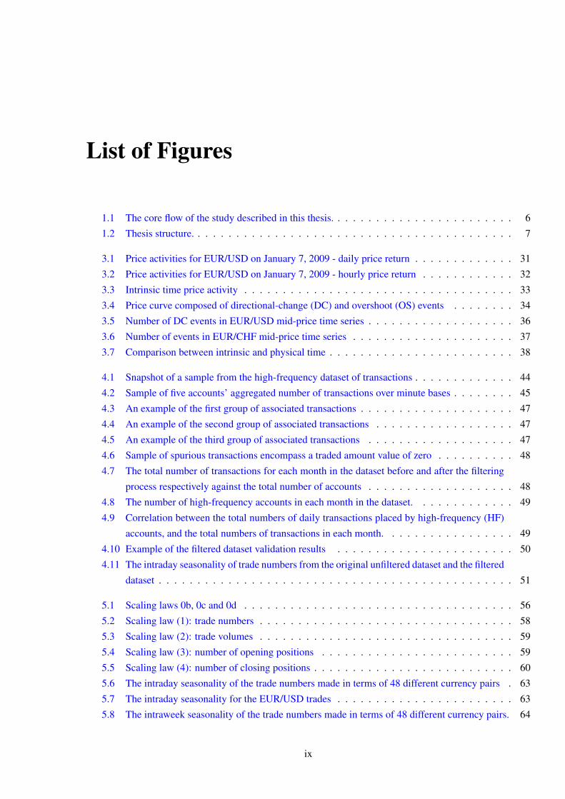
List of Figures
1.1 The core flow of the study described in this thesis. . . . . . . . . . . . . . . . . . . . . . . . 6
1.2 Thesis structure. . . . . . . . . . . . . . . . . . . . . . . . . . . . . . . . . . . . . . . . . . 7
3.1 Price activities for EUR/USD on January 7, 2009 - daily price return . . . . . . . . . . . . . 31
3.2 Price activities for EUR/USD on January 7, 2009 - hourly price return . . . . . . . . . . . . 32
3.3 Intrinsic time price activity . . . . . . . . . . . . . . . . . . . . . . . . . . . . . . . . . . . 33
3.4 Price curve composed of directional-change (DC) and overshoot (OS) events . . . . . . . . 34
3.5 Number of DC events in EUR/USD mid-price time series . . . . . . . . . . . . . . . . . . . 36
3.6 Number of events in EUR/CHF mid-price time series . . . . . . . . . . . . . . . . . . . . . 37
3.7 Comparison between intrinsic and physical time . . . . . . . . . . . . . . . . . . . . . . . . 38
4.1 Snapshot of a sample from the high-frequency dataset of transactions . . . . . . . . . . . . . 44
4.2 Sample of five accounts’ aggregated number of transactions over minute bases . . . . . . . . 45
4.3 An example of the first group of associated transactions . . . . . . . . . . . . . . . . . . . . 47
4.4 An example of the second group of associated transactions . . . . . . . . . . . . . . . . . . 47
4.5 An example of the third group of associated transactions . . . . . . . . . . . . . . . . . . . 47
4.6 Sample of spurious transactions encompass a traded amount value of zero . . . . . . . . . . 48
4.7 The total number of transactions for each month in the dataset before and after the filtering
process respectively against the total number of accounts . . . . . . . . . . . . . . . . . . . 48
4.8 The number of high-frequency accounts in each month in the dataset. . . . . . . . . . . . . 49
4.9 Correlation between the total numbers of daily transactions placed by high-frequency (HF)
accounts, and the total numbers of transactions in each month. . . . . . . . . . . . . . . . . 49
4.10 Example of the filtered dataset validation results . . . . . . . . . . . . . . . . . . . . . . . 50
4.11 The intraday seasonality of trade numbers from the original unfiltered dataset and the filtered
dataset . . . . . . . . . . . . . . . . . . . . . . . . . . . . . . . . . . . . . . . . . . . . . . 51
5.1 Scaling laws 0b, 0c and 0d . . . . . . . . . . . . . . . . . . . . . . . . . . . . . . . . . . . 56
5.2 Scaling law (1): trade numbers . . . . . . . . . . . . . . . . . . . . . . . . . . . . . . . . . 58
5.3 Scaling law (2): trade volumes . . . . . . . . . . . . . . . . . . . . . . . . . . . . . . . . . 59
5.4 Scaling law (3): number of opening positions . . . . . . . . . . . . . . . . . . . . . . . . . 59
5.5 Scaling law (4): number of closing positions . . . . . . . . . . . . . . . . . . . . . . . . . . 60
5.6 The intraday seasonality of the trade numbers made in terms of 48 different currency pairs . 63
5.7 The intraday seasonality for the EUR/USD trades . . . . . . . . . . . . . . . . . . . . . . . 63
5.8 The intraweek seasonality of the trade numbers made in terms of 48 different currency pairs. 64
ix

LIST OF FIGURES x
5.9 The intraweek seasonality for the EUR/USD trades . . . . . . . . . . . . . . . . . . . . . . 64
5.10 The correlation of EUR/USD trading activity . . . . . . . . . . . . . . . . . . . . . . . . . 66
6.1 The main components of the ABFXM and their interaction. . . . . . . . . . . . . . . . . . . 70
6.2 The platform’s main screen . . . . . . . . . . . . . . . . . . . . . . . . . . . . . . . . . . . 82
6.3 The market and traders parameters windows. . . . . . . . . . . . . . . . . . . . . . . . . . 83
6.4 The market-maker parameters windows. . . . . . . . . . . . . . . . . . . . . . . . . . . . . 83
6.5 The currency-pair parameters window. . . . . . . . . . . . . . . . . . . . . . . . . . . . . . 84
6.6 Intraday and intraweek seasonality of EUR/USD trades from the real data and the simulation
results. . . . . . . . . . . . . . . . . . . . . . . . . . . . . . . . . . . . . . . . . . . . . . . 89
6.7 Scaling laws of EUR/USD transactions for (a) the real data and (b) the simulation results . . 91
7.1 Intraday seasonality of trade numbers from the simulation results for different number of
agents . . . . . . . . . . . . . . . . . . . . . . . . . . . . . . . . . . . . . . . . . . . . . . 95
7.2 Intraday seasonality of trade volumes from the simulation results for different number of
agents . . . . . . . . . . . . . . . . . . . . . . . . . . . . . . . . . . . . . . . . . . . . . . 95
7.3 Scaling laws are plotted from simulation results for different total number of agents . . . . . 97
7.4 Intraday seasonality of trade numbers without the INAC. . . . . . . . . . . . . . . . . . . . 98
7.5 Scaling laws are plotted from simulation results without the activation of the initial condition
being set up . . . . . . . . . . . . . . . . . . . . . . . . . . . . . . . . . . . . . . . . . . . 100
7.6 Intraday seasonality of trade numbers and volumes from the simulation results without the
limit orders being generated . . . . . . . . . . . . . . . . . . . . . . . . . . . . . . . . . . 101
7.7 Scaling laws are plotted from simulation results without limit orders being generated . . . . 101
7.8 Intraday seasonality of trade numbers and volumes from two different settings for the initial
wealth distribution in the simulation . . . . . . . . . . . . . . . . . . . . . . . . . . . . . . 103
7.9 Scaling laws are plotted from the simulation results with different settings for the initial
wealth distribution . . . . . . . . . . . . . . . . . . . . . . . . . . . . . . . . . . . . . . . 104
7.10 Intraday seasonality of trade numbers and volumes from two different settings of the simu-
lation run for the distribution of the agents’ profit objectives . . . . . . . . . . . . . . . . . 106
7.11 Scaling laws are plotted from two different settings of the simulation run for the distribution
method for the agents’ profit objectives . . . . . . . . . . . . . . . . . . . . . . . . . . . . 107
7.12 Intraday seasonality of trade numbers and volumes from the simulation results with different
settings of the agents’ risk appetites . . . . . . . . . . . . . . . . . . . . . . . . . . . . . . 109
7.13 Scaling laws are plotted from the simulation results with different settings of the agents’ risk
appetites . . . . . . . . . . . . . . . . . . . . . . . . . . . . . . . . . . . . . . . . . . . . . 110
7.14 he intraday seasonality of trade numbers with the inclusion of heterogeneity in terms of the
agents’ adopted trading strategies . . . . . . . . . . . . . . . . . . . . . . . . . . . . . . . . 113
7.15 Scaling laws are plotted from the simulation results with different settings of the agents’
trading strategies . . . . . . . . . . . . . . . . . . . . . . . . . . . . . . . . . . . . . . . . 115
7.16 Intraday seasonality of trade numbers from the simulation results, without incorporating the
role of FX market trading sessions. . . . . . . . . . . . . . . . . . . . . . . . . . . . . . . . 117
7.17 Scaling laws are plotted from the simulation results without incorporating the role of FX
market trading sessions . . . . . . . . . . . . . . . . . . . . . . . . . . . . . . . . . . . . . 118

LIST OF FIGURES xi
7.18 Intraday seasonality of trade numbers and volumes from the simulation results with two
different settings of the order size parameter . . . . . . . . . . . . . . . . . . . . . . . . . . 120
7.19 Scaling laws are plotted from the simulation results with two different settings of the order
size parameter . . . . . . . . . . . . . . . . . . . . . . . . . . . . . . . . . . . . . . . . . . 122
8.1 The Backus Naur Form (BNF) of a decision tree. . . . . . . . . . . . . . . . . . . . . . . . 130
8.2 Example of a decision tree and a decision rule derived from the decision tree. . . . . . . . . 130
8.3 The intraday seasonality of the trade numbers from the different data samples . . . . . . . . 136
8.4 Scaling laws (1) from the different data samples . . . . . . . . . . . . . . . . . . . . . . . . 140
8.5 Scaling laws (2) from the different data samples . . . . . . . . . . . . . . . . . . . . . . . . 141
8.6 Scaling laws (3) from the different data samples . . . . . . . . . . . . . . . . . . . . . . . . 142
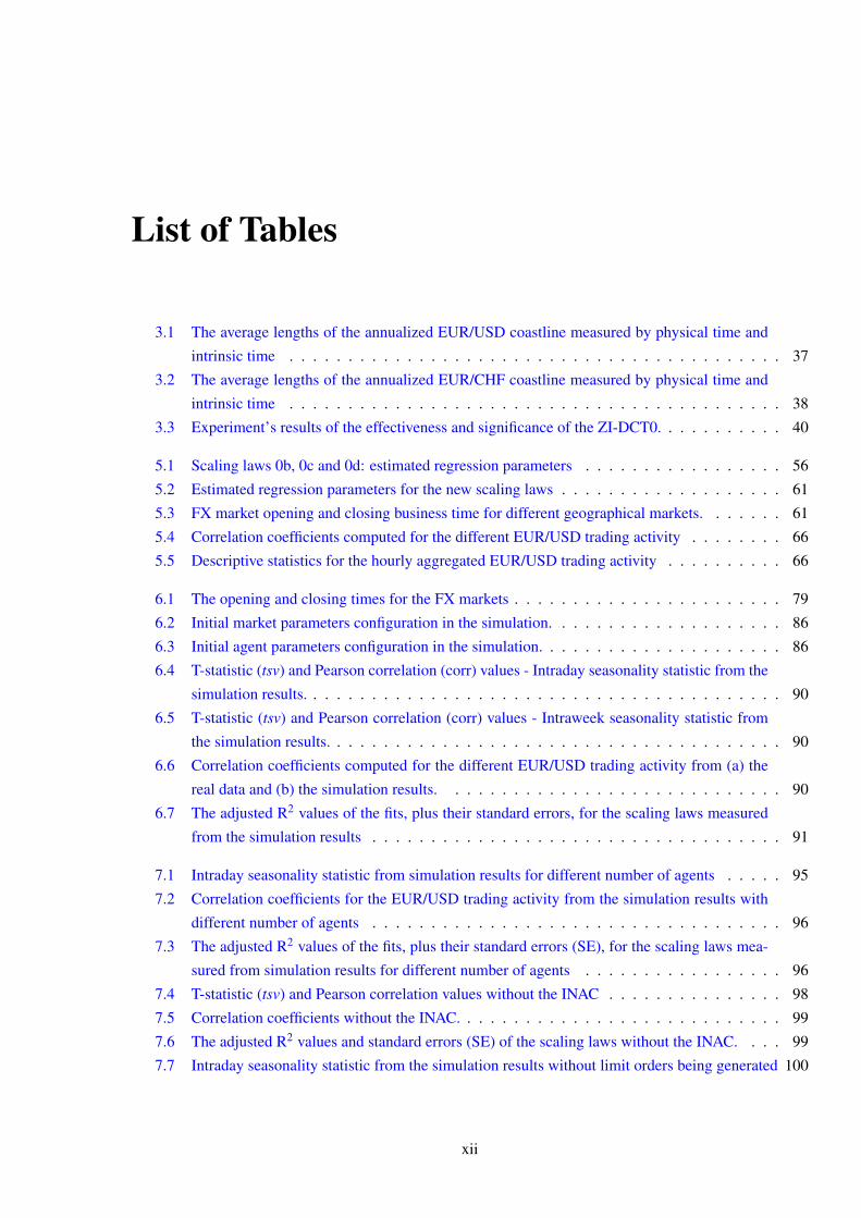
List of Tables
3.1 The average lengths of the annualized EUR/USD coastline measured by physical time and
intrinsic time . . . . . . . . . . . . . . . . . . . . . . . . . . . . . . . . . . . . . . . . . . 37
3.2 The average lengths of the annualized EUR/CHF coastline measured by physical time and
intrinsic time . . . . . . . . . . . . . . . . . . . . . . . . . . . . . . . . . . . . . . . . . . 38
3.3 Experiment’s results of the effectiveness and significance of the ZI-DCT0. . . . . . . . . . . 40
5.1 Scaling laws 0b, 0c and 0d: estimated regression parameters . . . . . . . . . . . . . . . . . 56
5.2 Estimated regression parameters for the new scaling laws . . . . . . . . . . . . . . . . . . . 61
5.3 FX market opening and closing business time for different geographical markets. . . . . . . 61
5.4 Correlation coefficients computed for the different EUR/USD trading activity . . . . . . . . 66
5.5 Descriptive statistics for the hourly aggregated EUR/USD trading activity . . . . . . . . . . 66
6.1 The opening and closing times for the FX markets . . . . . . . . . . . . . . . . . . . . . . . 79
6.2 Initial market parameters configuration in the simulation. . . . . . . . . . . . . . . . . . . . 86
6.3 Initial agent parameters configuration in the simulation. . . . . . . . . . . . . . . . . . . . . 86
6.4 T-statistic (tsv) and Pearson correlation (corr) values - Intraday seasonality statistic from the
simulation results. . . . . . . . . . . . . . . . . . . . . . . . . . . . . . . . . . . . . . . . . 90
6.5 T-statistic (tsv) and Pearson correlation (corr) values - Intraweek seasonality statistic from
the simulation results. . . . . . . . . . . . . . . . . . . . . . . . . . . . . . . . . . . . . . . 90
6.6 Correlation coefficients computed for the different EUR/USD trading activity from (a) the
real data and (b) the simulation results. . . . . . . . . . . . . . . . . . . . . . . . . . . . . 90
6.7 The adjusted R2 values of the fits, plus their standard errors, for the scaling laws measured
from the simulation results . . . . . . . . . . . . . . . . . . . . . . . . . . . . . . . . . . . 91
7.1 Intraday seasonality statistic from simulation results for different number of agents . . . . . 95
7.2 Correlation coefficients for the EUR/USD trading activity from the simulation results with
different number of agents . . . . . . . . . . . . . . . . . . . . . . . . . . . . . . . . . . . 96
7.3 The adjusted R2 values of the fits, plus their standard errors (SE), for the scaling laws mea-
sured from simulation results for different number of agents . . . . . . . . . . . . . . . . . 96
7.4 T-statistic (tsv) and Pearson correlation values without the INAC . . . . . . . . . . . . . . . 98
7.5 Correlation coefficients without the INAC. . . . . . . . . . . . . . . . . . . . . . . . . . . . 99
7.6 The adjusted R2 values and standard errors (SE) of the scaling laws without the INAC. . . . 99
7.7 Intraday seasonality statistic from the simulation results without limit orders being generated 100
xii

LIST OF TABLES xiii
7.8 Correlation coefficients for the EUR/USD trading activity from the simulation results with-
out limit orders being generated . . . . . . . . . . . . . . . . . . . . . . . . . . . . . . . . 101
7.9 The adjusted R2 values of the fits, plus their standard errors, for the scaling laws measured
from the simulation results without limit orders being generated . . . . . . . . . . . . . . . 102
7.10 Intraday seasonality statistic from two different settings for the initial wealth distribution in
the simulation . . . . . . . . . . . . . . . . . . . . . . . . . . . . . . . . . . . . . . . . . . 103
7.11 Correlation coefficients of the EUR/USD trading activities from the simulation results with
different settings for the initial wealth distribution . . . . . . . . . . . . . . . . . . . . . . . 103
7.12 The adjusted R2 values of the fits, plus their standard errors, for the scaling laws measured-
from the simulation results with different settings for the initial wealth distribution . . . . . 105
7.13 Intraday seasonality statistic for two different settings of the simulation for the distribution
of the agents’ profit objectives . . . . . . . . . . . . . . . . . . . . . . . . . . . . . . . . . 106
7.14 Correlation coefficients for the EUR/USD trading activity for two different settings of the
simulation run for the distribution of the agents’ profit objectives . . . . . . . . . . . . . . . 106
7.15 The adjusted R2 values of the fits, plus their standard errors (SE), for the scaling laws mea-
sured from two different settings of the simulation run for the distribution method for the
agents’ profit objectives . . . . . . . . . . . . . . . . . . . . . . . . . . . . . . . . . . . . . 108
7.16 Intraday seasonality statistic of trade numbers and volumes from the simulation results with
different settings of the agents’ risk appetites . . . . . . . . . . . . . . . . . . . . . . . . . 109
7.17 Correlation coefficients for the EUR/USD trading activity from the simulation results with
different settings of the agents’ risk appetites . . . . . . . . . . . . . . . . . . . . . . . . . 110
7.18 The adjusted R2 values of the fits, plus their standard errors, for the scaling laws measured
from the simulation results with different settings of the agents’ risk appetites . . . . . . . . 111
7.19 Basic descriptive statistics of the agents’ ROI from four independent runs of the simulation . 112
7.20 T-statistic (tsv) and Pearson correlation (corr) values with the inclusion of heterogeneity in
terms of the agents’ adopted trading strategies . . . . . . . . . . . . . . . . . . . . . . . . . 114
7.21 Correlation coefficients for the EUR/USD trading activity from three different simulation
results with the inclusion of heterogeneity in terms of the agents’ adopted trading strategies. 114
7.22 The adjusted R2 values of the fits, plus their standard errors, for the scaling laws measured
from five different simulation results with the inclusion of heterogeneity in terms of the
agents’ adopted trading strategies . . . . . . . . . . . . . . . . . . . . . . . . . . . . . . . . 114
7.23 Intraday seasonality statistic from simulation results without incorporating the role of FX
market trading sessions . . . . . . . . . . . . . . . . . . . . . . . . . . . . . . . . . . . . . 117
7.24 Correlation coefficients for the EUR/USD trading activity from the simulation results with-
out incorporating the role of FX market trading sessions . . . . . . . . . . . . . . . . . . . . 117
7.25 The adjusted R2 values of the fits, plus their standard errors, for the scaling laws measured
from the simulation results without incorporating the role of FX market trading sessions . . 118
7.26 Intraday seasonality statistic from the simulation results with two different settings of the
order size parameter . . . . . . . . . . . . . . . . . . . . . . . . . . . . . . . . . . . . . . . 120
7.27 Correlation coefficients for the EUR/USD trading activity from the simulation results with
two different settings of an agents order size parameter . . . . . . . . . . . . . . . . . . . . 121

LIST OF TABLES xiv
7.28 The adjusted R2 values and standard errors of the scaling law fits from the simulation results
with two different settings of the order size parameter . . . . . . . . . . . . . . . . . . . . . 121
8.1 The indicators used by GPAs to form decision rules and their respective short and long-term
periods. . . . . . . . . . . . . . . . . . . . . . . . . . . . . . . . . . . . . . . . . . . . . . 132
8.2 Initial configuration for for the GP parameter values used for the GPAs. . . . . . . . . . . . 135
8.3 T-statistic and Pearson correlation from the different data samples . . . . . . . . . . . . . . 137
8.4 Correlation coefficients computed for the different EUR/USD trading activity from the dif-
ferent data samples . . . . . . . . . . . . . . . . . . . . . . . . . . . . . . . . . . . . . . . 138
8.5 The adjusted R2 values of the fits, plus their standard errors, for the scaling laws from the
different data samples . . . . . . . . . . . . . . . . . . . . . . . . . . . . . . . . . . . . . . 139
8.6 Descriptive statistics of the agents’ ROI from the different data samples . . . . . . . . . . . 143

Chapter 1
Introduction
1.1 Motivation
Classical theories of economics are founded on strong assumptions such as perfect rationality, homogeneity
and efficient market hypothesis [25, 59, 61, 79]. Some of these assumptions used in classical economic
theories are flawed. Classical economic theories fail to explain the dynamics of financial market behaviour
and the forces that drive such behaviour [33, 102, 148, 155, 156, 216, 220]. In order to better understand
and analyse financial and other markets, researchers attempt to identify patterns in the data. The observed
statistical properties of the financial market data are referred to as stylized facts [63]. The variance between
classical economics theories and the empirical stylized facts observed in financial markets data are the main
driving force for the development and the usage of different approaches to studying the behaviour of such
markets. For instance, the concept of bounded rationality has exclusively replaced the concept of full rational
homogeneous representative agents [20, 21, 204–206]. Such a change in conception motivates the need to
study and revise some of the existing economic theories which are based upon many idealised assumptions.
Three major approaches have been used to study and analyse the behaviour of the Foreign Exchange
(FX) market in the literature: behavioural finance, analytical models and agent-based modelling. The be-
havioural finance approach is a theory which employs psychology to explore and describe the behaviour
of financial market traders and their behavioural influence on the market dynamics. A good review of
behavioural finance is provided in [29, 203, 211]. A substantial number of studies have established the
existence of several psychological underpinnings for FX market traders’ behaviour. For example, these in-
clude studies of financial market traders’ herding behaviour [125], feedback trading in the market [1, 38,
136], traders’ heterogeneous expectations and beliefs [87, 88, 116, 162, 173, 178], traders’ overconfidence
[28, 97, 179], and loss aversion bias [180]. The second approach employs analytical models to study FX
market behaviour. A number of studies in this area, have considered the effect of order flow [34, 75, 77],
market news arrival [10, 14, 47, 76, 78], fundamentals trading on price movements [75, 78], and behaviour
of market participants. The major weakness of the analytical models is the lack of direct insight into the
microscopic nature of the market stylized facts [131].
Due to the current large number and complexity of financial market data, especially high-frequency
data, compared to earlier times, traditional analytical models present some difficulties in analysing finan-
cial market behaviour [172]. Agent-based markets (ABMs) have emerged as an alternative approach for
exploring and studying dynamic behaviour in financial and other markets, especially where the application
of analytical models is difficult and their use may be not be able to yield satisfactory results or useful in-
1

CHAPTER 1. INTRODUCTION 2
sights [172]. An ABM uses computer programs to model the behaviour of a real market which is made up
of various aspects such as a trading mechanism, traded assets and trading agents that may emulate human
traders. The ABM approach has been successfully applied in different financial studies, from macroeco-
nomic models to payment card markets [2, 15, 17, 126, 129]. A good introduction to ABMs can be found
in [214]. For an overview of the most influential works in the field of ABMs, we refer interested readers to
[62, 137, 143, 193].
ABMs that emulate the behaviour of real markets need to be modelled in such a way so as to exhibit
the same stylized facts as real ones [143]. In an ABM, the observation of the same stylized facts as the real
market serves as a useful benchmark and as evidence that the ABM is indeed closely modelling the real
market with a high degree of confidence. ABMs that exhibit the same stylized facts as real markets can be
used to identify and interpret their origins through comprehensive experimentation; this can provide useful
insights into the workings of the real market, the forces that drive behaviour and their impact on the market
dynamics which would not otherwise be possible [138]. A number of ABMs have been able to exhibit some
of the markets’ stylized facts [5–7, 21, 42, 46, 48, 49, 56, 64, 83, 95, 114, 128, 138, 145, 146, 149, 150, 153,
158, 159, 170, 172, 215, 232, 238], whereas only some of these ABMs have clearly defined and interpreted
the origins of the market stylized facts, such as the work in [5–7, 64, 172].
Although ABMs offer a number of advantages in modelling markets, the use of ABMs has been criti-
cized from a number of viewpoints and in particular with regard to the complexity of these ABMs, the prob-
lem of calibration, the numerous parameters needed for developing the ABM, etc. [96, 137, 141, 143, 230].
Despite the existence of previous or contemporary studies on modelling financial markets using ABMs, a
number of issues have not been well-studied or properly addressed as yet:
• Although there are many different works which have studied the trading activity in the FX market,
there has been no systematic study of its properties using a high-frequency dataset and an ABM.
Previous studies of the FX markets have acquired either large samples of low frequency datasets [77],
or small samples of high-frequency datasets [34], neither of which are at the account level. In finance,
high-frequency data represent an extremely large amount of data which is the full historical record of
transactions in the market, and the characteristics associated with transactions at frequencies higher
than on a daily basis [74]. A systematic exploration of properties of the trading activity in the FX
market requires the use of a high-frequency dataset of individual traders’ historical transactions over
a substantially long period of time.
• ABMs have generally aimed at reproducing some of the stylized facts of financial markets such as
[5–7, 21, 42, 46, 48, 49, 56, 64, 83, 95, 114, 128, 138, 145, 146, 149, 150, 153, 158, 159, 170, 172,
215, 232, 238]. However, many of these studies such as [21, 48, 146, 150, 232] pay little attention
to identifying and understanding the origins of the market stylized facts. For instance, the authors
of the Santa Fe Artificial Stock Market (SF ASM) do not provide a quantitative description of the
reproduced stylized facts, neither do they explain the dynamics of the self-organization of the markets
[21, 146]. LeBaron suggested that, “It is important in agent based models not just to reproduce
features of real markets, but also to show which aspects of the model may have led to them” ([138],
p. 226). Examples of ABMs that attempt to explain the origin of stylized facts of the price returns
are [5–7, 64, 172]. Alfi et al. in [5–7] present an ABM containing the simplest possible elements to
define and understand the origin of the stylized facts of price returns. In contrast, Martinez-Jaramillo
and Tsang in [171, 172] model a simple market mechanism of a stock market which operated with
CHAPTER 1. INTRODUCTION 3
sophisticated genetic programming based agents. Their work identifies the minimal set of essential
conditions under which the stylized facts of endogenously generated prices resemble those of real
market prices. The work done by Daniel in [64] focuses on the intraday stylized facts of order flow
and price returns in the stock market. Daniel studies the origin of the stylized facts using a double
auction market mechanism operated with zero-intelligence models of agents.
• To the best of our knowledge, none of the previous studies have identified the essential elements
under which the stylized facts of the trading activity in the high-frequency FX market-makers markets
emerge in an ABM. The FX market is the largest financial market in the world with a high volume of
transactions and a high level of liquidity [63]. To acquire an understanding of the dynamics of trading
behaviour in the high-frequency FX market, it is essential to define and understand the origin of the
trading activity in the market, and the forces that drive the flow of the market trading activity which
may be far from traditional assumptions of economics.
• Although ABMs are a powerful tool for modelling markets and understanding their behaviour, they
have often been criticised for the level of complexity involved in their set up [110]. Developers
are faced with a daunting set of design choices [137]. Simplicity is essential in designing ABMs
[110, 143, 193] as a complex design may impede the study, understanding and interpretation of the
origins of the stylized facts [110]. Although it is often tempting to develop ABMs with intricate
set ups and numerous composite parameters, such often unwarranted complexity makes it difficult
to identify which elements of the market are accountable for the emergence of the stylized facts and
whether all of the elements are equally important for reproducing them [143].
• One of the issues in ABMs is that of validation [96, 137, 141, 143, 230]. Constructed ABMs need
to be able to reproduce to a satisfactory extent the same behaviour as the corresponding real markets.
Therefore establishing the stylized facts of the real market is essential for providing a benchmark for
ABMs [137, 141, 143, 146]. Otherwise, the validity of any theoretical results drawn from ABMs
would be of concern. However, in order to establish stylized facts for a market, one needs to have
access to real market data, in particular high-frequency data, and the problem is the lack of such
market data.
• Defining the parameter space in an ABM is a daunting task as the parameter space can be very big.
LeBaron explained that "... understanding exactly where the parameter boundaries are between simple
and complex behaviors is crucial to understanding the mechanisms that drive agent based markets"
([137], p. 258).
• Timing is an important design issue in terms of building ABMs. In some ABMs, trading is synchro-
nized and there are no representations of physical time [18, 21, 150, 170, 172, 238]. In addition,
some ABMs employ low-frequency timing where each trading round corresponds to one simulated
day which doesn’t reflect real markets [172].
1.2 Aim and Objectives
This thesis aims to identify and study the essential elements under which the stylized facts of the trading
activity in the high-frequency FX market emerge in the context of an ABM. This aim is comprised of the

CHAPTER 1. INTRODUCTION 4
following major objectives:
• To identify a number of stylized facts that characterise the trading activity in the high-frequency FX
markets which can serve as a benchmark for validating ABMs. This foundational step includes the
acquiring of a high-frequency dataset of individual traders’ historical transactions in the FX market.
Such a dataset permits us to conduct an analysis of the FX market traders’ collective behaviour in
order to establish a set of stylized facts.
• To define and construct an agent-based FX market (ABFXM) that simulates the trading activity at the
level of an FX market-maker market. The ABFXM should be able to reproduce the stylized facts of
the trading activity as exhibited in the real FX market to a satisfactory extent.
• To model individual heterogeneous trading agents. The design and structure of the agents should be
as simple as possible, and with the minimal number of elements which, at the same time, are still
able to reproduce the stylized facts of the FX market trading activity. Simplicity allows for a detailed
and clear interpretation of the origin of the market stylized facts in isolation from complex trading
behaviour. Heterogeneity is inherent in real markets where participants have different preferences,
demands, aspirations, trading strategies and trading hours.
• To evaluate the ABFXM. The ABFXM that is to be developed must be thoroughly evaluated in order
to ascertain the ability of the ABFXM to approximate the stylized facts of the trading activity of the
FX market.
• To examine in a systematic manner the impact of changes in different elements of the ABFXM on
the emergence of the trading activity stylized facts in the FX market. Such an examination results
in a comprehensive search for a set of essential elements under which the stylized facts of the high-
frequency FX market trading activity emerge in an ABM.
• To study and explore impact of different trading strategies in the market and on the emergence of the
trading activity stylized facts in the FX market.
1.3 Thesis Overview
To model the trading activity in the FX markets, we use two different approaches: the analysis of actual
traders’ behaviour and ABM. We start from the analysis of actual traders’ behaviour moving towards the
agent-based models. Such a combination allows us to achieve a good understanding in terms of both theory
and practice of the behaviour of the trading activity in the FX markets.
Figure 1.1 depicts the core flow of the study described in this thesis. The initial part of this study is to
establish a number of stylized facts that characterise the trading activity in FX markets, using a unique high-
frequency dataset of traders’ historical transactions. The dataset is provided by the OANDA Corporation. To
the best of our knowledge, this dataset is considered to be the largest available high-frequency dataset of FX
market traders’ historical transactions. Prior to the analysis of the dataset, we conduct a filtering procedure
to remove any possible misleading and spurious transactions in terms of the traders’ actual activity. We build
an ABFXM which overcomes the limitations and issues discussed above (section 1.1), aiming at reproducing
the stylized facts of the real FX market’s trading activity. Using the identified stylized facts as a benchmark,

CHAPTER 1. INTRODUCTION 5
we evaluate the trading activity reproduced from the ABFXM. A systematic exploration of the implications
of varying the features and parameters of the ABFXM is undertaken. The aim is to identify the essential
elements involved in our ABFXM which are responsible for reproducing the stylized facts of the trading
activity in the FX markets.
Our work is different from the work done in [5–7, 21, 42, 46, 48, 49, 56, 64, 83, 95, 114, 128, 138, 145,
146, 149, 150, 153, 158, 159, 170, 172, 215, 232, 238], in that we used an agent-based approach to model
trading behaviour in the high-frequency FX market and investigate the emergence of the stylized facts of
transactions data in a systematic way. We have been able to study extensively the effect of each of the
constituent elements of the ABFXM on the stylized facts through anchoring the simulation results by using
a historical high-frequency prices dataset. The use of this dataset enables us to run multiple simulation runs
and draw comparisons and conclusions for each market setting against the real data but also by comparing
different market settings against each other. As far as we know, this has not been done before.
To the best of our knowledge, the work presented in this thesis is the first study which has attempted to
identify and understand the design effect of the agents’ trading strategy in the emergence of the FX market
stylized facts. Our work is different from the studies done in [54, 99, 189, 225] in four major aspects. Firstly,
we examine three alternative approaches to the design of the agents’ strategies, two of which are commonly
used for modelling agents in ABMs. Secondly, we examine the impact of the design of the agent’s trading
strategy in the emergence of the trading activity stylized facts in the high-frequency FX market, rather that
examining the impact on the market mechanism as done in [54, 99, 225] or on the stylized facts of the order
flow as done in [189]. Thirdly, our study focuses on the FX market, while the studies in [54, 99, 189] use a
double auction market and the study in [225] uses a web-based prediction market platform. Finally, to our
knowledge, this is the first study that uses a unique high-frequency dataset of individual traders’ historical
transactions to validate the results of the ABFXM.
1.4 Thesis Structure
The thesis structure is depicted in Figure 1.2 and is as follows. Chapter 2 provides an introduction in terms
of a background to the study and an outline literature review of the financial markets and, in particular,
the FX markets. In this chapter, we present references to some of the important studies into the behaviour
of the FX markets’ traders. Nevertheless, it is not our intention to provide a comprehensive review of the
literature regarding the FX markets. Furthermore, chapter 2 reviews the literature with regard to ABMs.
In this chapter, we review some of the important and most promising studies that have been undertaken
in ABMs and which we consider relevant to the study presented in this thesis. In addition, this chapter
illustrates artificial intelligence techniques in general, and evolutionary computation in particular, that are
used in financial forecasting. We conclude this chapter by describing the high-frequency data of financial
markets; show their potential usefulness, and consider the challenges associated with dealing with them.
Financial markets witness high levels of activity at certain times, but remain calm at others. This makes
the flow of physical time discontinuous. Therefore, using physical time scales for studying financial time
series runs the risk of missing important periods of activity in the markets. An alternative approach is the
use of an event-based time that captures periodic activities in the market. Chapter 3 describes a special
type of event, called a directional-change event which can be used for studying financial time series. In this
chapter, we show the potential usefulness of this approach in terms of capturing periodic market activities.

CHAPTER 1. INTRODUCTION 6
Figure 1.1: The core flow of the study described in this thesis.

CHAPTER 1. INTRODUCTION 7
Figure 1.2: Thesis structure.
We measure the length of the price curve coastline, which represents the profit potential, as defined by
directional-change events, as well as physical time scales. Furthermore, in chapter 3, we construct a new
trading strategy based on the directional-change event approach. A series of controlled experiments were
conducted aiming to study the impact of such a trading strategy on a trader’s performance.
In chapter 4, we process a unique high-frequency dataset representing the full transaction history of more
than 40,000 anonymised accounts on the OANDA FX trading platform over 2.25 years. Prior to exploring
and analysing the data to discover and define the stylized facts of the trading activity in the FX market, we
perform a filtering procedure to remove misleading and spurious data from the dataset that would affect the
validity of any forthcoming results. We conclude chapter 4 by validating the adopted filtering procedure and
showing the behaviour and effects of the filtered dataset.
Chapter 5 describes a benchmark for validating FX market agent-based models. In this chapter we
conduct an analysis of the trading activity in the OANDA FX trading platform using the high-frequency
dataset of individual traders’ historical transactions. This allows us to establish a set of stylized facts which
characterize the trading activity of the FX market and apply on transactions data. These established stylized
facts can be grouped under three main headings: scaling laws, seasonality and correlation behaviour. These
independent stylized facts describe the trading activity in the FX market from different angles.
Chapter 6 describes the development of the ABFXM. It begins with describing the ABFXM mechanism,
CHAPTER 1. INTRODUCTION 8
and the available traded assets in the market. Then it describes the design and structure of the trading
agents, the trading cycle and the market clearance. Later on in this chapter, the computational platform
of the ABFXM is briefly described together with a description of the flexibility and extensibility of the
ABFXM. Furthermore, chapter 6 reports the experimental and validation design to validate the precision of
the ABFXM in reproducing the stylized facts of trading activity as exhibited in the real high-frequency FX
market. The results of the experiments that have been performed are presented to confirm the validity of the
ABFXM.
Chapter 7 offers a detailed examination and exploration of the implications of changing some of the
elements of the ABFXM presented in chapter 6. A systematic approach is used due to the different possible
combinations of the elements involved in the ABFXM. Accordingly, in this chapter, we draw conclusions
on what seem to be the important elements of the ABFXM that lead to the emergence of the stylized facts
in the high-frequency FX market.
One of the most critical design issues that developers face in electronic markets is that of the agents’
trading strategies. In chapter 8, we examine the impact of trading strategies on the high-frequency FX
market. In particular, our goal is to explore the emergence of the stylized facts in the trading activity under
different settings where the market is populated with agents with three different strategies: a variation of
the zero-intelligence with a constraint (ZI-CV) strategy; the zero-intelligence directional-change event (ZI-
DCT0) strategy; and the genetic programming-based (GP) strategy.
The thesis concludes with chapter 9 which provides a summary of the thesis, lists its main contributions,
and proposes possible avenues for future work.
1.5 Publications
The work presented in this thesis has led to the following publications:
• Aloud, M., E. Tsang, R. Olsen, and A. Dupuis (2012), A directional-change events approach for
studying financial time series, Economics: The Open-Access, Open-Assessment E-Journal, 6 (36).
http://dx.doi.org/10.5018/economics-ejournal.ja.2012-36
• Aloud, M., E. Tsang, and R. Olsen (2012), Modelling the FX market traders’ behaviour: an agent-
based approach, Chapter 15, in Simulation in Computational Finance and Economics: Tools and
Emerging Applications, edited by B. Alexandrova-Kabadjova, S. Martinez-Jaramillo, A. Garcia-Almanza,
and E. Tsang, IGI Global, Hershey, Pennsylvania, 202-228.
• Aloud, M., and M. Fasli (2012), The impact of strategies on the stylized facts in the FX market, Tech.
rep. CES-528, University of Essex, United Kingdom.
• Aloud, M., M. Fasli, E. Tsang, A. Dupuis, and R. Olsen (2012), Modelling the high-frequency FX
market: an agent-based approach, Tech. Rep. CES-519, University of Essex, United Kingdom.
• Aloud, M., M. Fasli, E. Tsang, A. Dupuis, and R. Olsen (2012), Stylized facts of trading activity in
the high frequency FX market: An Empirical Study, Tech. Rep. CES-520, University of Essex, United
Kingdom.
CHAPTER 1. INTRODUCTION 9
• Aloud, M., and E. Tsang (2011), Modelling the trading behaviour in high-frequency markets, in 3rd
Computer Science and Electronic Engineering Conference (CEEC), IEEE Xplore, Colchester, United
Kingdom.
• Aloud, M., E. Tsang, A. Dupuis, and R. Olsen (2011), Minimal agent-based model for the origin of
trading activity in foreign exchange market, in IEEE Symposium on Computational Intelligence for
Financial Engineering & Economics, IEEE Xplore, Paris, France.
• Masry, S., M. Aloud, A. Dupuis, R. Olsen, and E. Tsang (2010), High frequency FOREX market
transaction data handling, in 4th CSDA International Conference on Computational and Financial
Econometrics, London, United Kingdom.
• Aloud, M., E. Tsang, and R. Olsen (2010), Definitions of directional-change events, in 2nd Computer
Science and Electronic Engineering Conference (CEEC), IEEE Xplore, Colchester, United Kingdom.
• Masry, S., M. Aloud, A. Dupuis, R. Olsen, and E. Tsang (2010), A novel approach for studying the
high-frequency FOREX market, in 2nd Computer Science and Electronic Engineering Conference
(CEEC), University of Essex, IEEE Xplore, Colchester, United Kingdom.

Chapter 2
Background and Literature Survey
2.1 Introduction
Financial markets are institutions whose objective is to facilitate the exchange of assets. Financial markets
allow trading in financial securities, commodities and other exchangeable assets, depending on the market
type and can be categorised into different groups, based on the type of traded asset. Some examples of
financial markets are: capital markets, commodity markets, stock markets, foreign exchange markets and
derivatives markets. For a good introductory reference to financial markets, we refer the interested reader
to [200]. In this thesis, we focus on studying the Foreign Exchange (FX) market. One of the important
research activities associated with financial markets is to define and explain the origin and nature of trading
activities in these markets.
In this chapter, it is not our intention to provide a broad overview neither of the financial markets nor of
the FX market. This chapter aims to explain the Efficient Market Hypothesis (EMH) (section 2.2); present
the common stylized facts of financial assets (section 2.3); provide an overview of the FX market structure
(section 2.4); present an outline of the empirical studies of FX market behaviour (section 2.5). In this
chapter, we review the state of the art in agent-based markets (ABMs) (section 2.6). We start by providing
an overview of some ABMs which are relevant to our work. In section 2.7, we describe and survey the
design routes with regard to building an ABM. In section 2.8, we discuss artificial intelligence techniques in
general, and evolutionary computation in particular, that are used in financial forecasting. We conclude this
chapter by describing the high-frequency data and show their potential usefulness and challenges (section
2.9).
2.2 The Efficient Market Hypothesis
Many empirical financial economic studies in previous decades have engaged in an intense debate about the
concept of market efficiency [33, 102, 148, 155, 156, 216, 220]. The Efficient Market Hypothesis (EMH)
states that financial markets are "informationally efficient" if the price reflects all the available information
[80]. In terms of the EMH, the information set is considered to be anything that may possibly affect the
movement of an asset’s price. Based on the information set available, there are three common forms of
the EMH [68]: the Weak Form Efficiency hypothesis asserts that all relevant available information is fully
reflected in current and historical asset prices. The Semi-Strong Form Efficiency hypothesis asserts that
all publicly available information is fully reflected in current and historical asset prices. The Strong Form
10

CHAPTER 2. BACKGROUND AND LITERATURE SURVEY 11
Efficiency hypothesis asserts that all information, including public and private information, is fully reflected
in current and historical asset prices.
In the past, the concept of market efficiency has indicated that price changes follow a random walk [163],
whereas the facts derived from the statistical analysis of the financial market data evidently now show the
opposite [155]. The random walk hypothesis states that asset returns are serially independent, which means
that they do not follow any trend or pattern. As a result, the next period return is not a result of the previous
ones [220]. In other words, historical data cannot be used to predict the future movements of the asset price
in such a way as to outperform the market. Many empirical studies have been conducted in order to examine
the concept of the EMH by explaining the behaviour of assets’ prices, such as [148, 156]. In addition, many
researchers such as [33, 102, 155, 216] have rejected the concept of EMH. Beyond the debates with regard
to EMH and the concept of a random walk, our work sheds some light into explaining patterns in price time
series and, most importantly, provides an explanation for the origins of some of the trading activity in the
FX market.
2.3 Stylized Facts of Asset Returns
Stylized facts of asset returns are the observed statistical properties of the time series of asset price returns.
Such stylized facts are considered to be common across a wide range of financial markets and time periods
[57]. They have become an important feature for researchers, which has led to a greater understanding of
financial market behaviour [63]. In building a model of the financial market, stylized facts are considered
to be the first verification criterion [142]. In addition, numerous financial market models have been built in
an attempt to reproduce and explain some of the stylized facts. Reproducing such stylized facts is not an
easy task, as noted by Cont ". . . these stylized facts are so constraining that it is not easy to exhibit even an
(ad hoc) stochastic process which possesses the same set of properties and one has to go to great lengths to
reproduce them with a model" ([57], p. 224). One of the most basic requirements when analyzing market
data is that the stylized facts remain stable over different periods, and there is a need to clearly identify
them. More specifically, it is necessary to ensure that a statistical property does not depend on a certain time
period, but it is observed at different times.
In most studies, the statistical analysis of the financial asset price time series is performed using the
continuously compounded return or log return [172]. The log return is defined as follows:
Rt ≡ log(Pt
Pt−1) = log(Pt)− log(Pt−1) (2.1)
where Rt denotes the return at time t, Pt denotes the price of an asset, a market stock, index or an
exchange rate, at time t.
The common stylized facts relevant to a broad set of financial assets, as described in detail in [57] are:
1. Absence of linear auto-correlation: (linear) autocorrelation of asset returns is usually insignificant,
but some correlations may be present for small intra-day time scales (minutes or less). This statistical
property corresponds to the state of an efficient market in which it is not possible to make a profit
without risk [5]. In addition, due to the lack of autocorrelation in returns, each return is considered to
be independent from the previous returns, giving support to the notion that prices perform a random
walk. One can verify if the generated asset price return from a certain market model shows evidence of
the absence of autocorrelation, by reporting the correlations of the log returns, the square log returns

CHAPTER 2. BACKGROUND AND LITERATURE SURVEY 12
and the absolute log returns for different time intervals. The log returns’ correlations should be around
zero for different time intervals if there is a lack of linear auto correlation [172]. Empirical studies
of various market data have been performed to test the absence of autocorrelation properties in asset
price return. Hsieh in [113] performed a study of the daily changes of five foreign exchange rates and
found evidence of no linear correlation. Brooks in [43] examined 10 daily Sterling exchange rates and
found that there was no linear autocorrelation in many of the time series. Ammermann and Patterson
[12] indicated that nonlinear serial dependencies are very important in the returns for a wide range of
financial time series.
2. Heavy tails: the (unconditional) distribution of returns displays a heavy tail with positive excess
kurtosis. In most assets, exchange rates and indexes, the tail index is finite, higher than two and less
than five. The heavy tail definition as noted by Martinez-Jaramillo and Tsang "The term “fat tails”
refers to higher density on the tails of a distribution in comparison to the tails’ density under the
normal distribution" ([172], p. 34). In order to quantify the deviation from the normal distribution,
one can report the log return’s kurtosis [57]. Kurtosis is commonly defined as the fourth central
moment of a distribution, and it measures the degree of flatness relative to a normal distribution and is
a useful indicator of fat tails [172]. The kurtosis of a normal distribution is three. In many empirical
studies of financial market data, it has been found that the sample kurtosis is larger than three, which
is known as excess kurtosis and is a signature of fat tails [172].
3. Conditional heavy tail: the residual time series exhibits heavy tails even after correcting returns for
volatility clustering, but the tails are less heavy than in the unconditional distribution of return. This
statistical property can be tested by reporting the sum of the ARCH and GARCH coefficients in which,
the closer the sum is to one, the more persistence of volatility, the more volatile the stocks are [172].
4. Volatility clustering: a different measure of volatility shows a positive correlation over a number of
days which quantifies that high-volatility events tend to cluster in time. According to Mandelbort
in [164]: ". . . large changes tend to be followed by large changes, of either sign, and small changes
tend to be followed by small changes". Volatility is considered to be the greatest puzzle in finance
and the difficulties associated with it was first demonstrated by Shiller in [201]. An update of this
report can be found in [142, 202]. The persistence of volatility in financial time series has lead to
an entire industry of models, ARCH by Engle in [73], GARCH by Bollerslev in [41], which aim
to describe several related effects to the phenomenon of financial volatility such as excess kurtosis
[142]. Volatility clustering can be measured through the use of the autocorrelation of the absolute and
squared log returns [164]. If such positive autocorrelations happen, then it is an obvious signature of
volatility clustering.
5. Volume/volatility correlation: studies show that the trading volume, the number of assets traded during
a specific period, is correlated with all measures of volatility.
6. Intermittency: financial asset returns shows a high degree of variability using any time scale.
7. Aggregational gaussianity: asset returns appear to be normally distributed over a long time period.
As a result, increasing the time scale results in their returns distribution looking increasingly like a
normal distribution. Moreover, the distribution varies between different time scales. One can indicate
CHAPTER 2. BACKGROUND AND LITERATURE SURVEY 13
whether the sampled market data is drawn from a normal distribution or not by performing the Jarque-
Bera test, which measures the departure from normality using the skewness and the kurtosis of the
sample data [172].
2.4 Overview of the FX Market
The Foreign Exchange market, also referred to as the Forex or FX market, is considered the largest and
most liquid financial market in the world [63]. The FX market is where the buying and selling of foreign
currencies takes place in order to facilitate the trade of a range of currencies around the world. Participants
in the FX market consist of governments, central banks, large banks, institutional investors, individual
investors, etc.
The FX market is not a single market, but is composed of a global network of FX markets that connect
investors from all around the world. The fact that the FX market is a decentralized market means that there
is no central marketplace, and that transactions are conducted over the counter. Most FX trading firms are
market-makers. The rapid advances in communications technology, particularly in web-related technology,
in the last two decades have led to huge changes in the FX market in that a number of independent brokers
have developed internet-based trading platforms - the so-called market-maker FX market. The role of the
electronic market-maker has increased rapidly in the last decade and electronic market-makers play an
important role in the growth of the financial market. With the advent of retail market-maker FX market
online platforms, individual retail traders represent an important part of the FX market.
A market-maker is an institution which provides liquidity for a number of currency pairs, and quotes
both a buy and a sell price on its platform in an attempt to make a profit through the bid/ask spread. In an FX
trading environment, the market-maker is equipped to buy from and sell to its investors and other market-
makers at those quoted bid and ask prices. In other words, the market-maker takes the opposite side of a
trade. The market-maker’s role is essential in maintaining the liquidity with regard to a given security that
is held in his inventory. A market-maker adjusts the price based on the demand and supply in the market, on
their inventory holdings, on news and prices from other market-makers, as well as other factors.
In contrast to stock markets, the FX market operates 24 hours a day, 7 days a week. Despite the fact that
the FX market operates continuously, 24 hours a day, the trading activity is not homogenous in time, which
leads to difficulties in analyzing the data [63]. The peak liquidity occurs when the business trading hours of
multiple time zones overlap [63]. It is essential to understand the correlation between market activity and
daytime over different periods of the day.
The characteristics of the FX market are, to some extent, different from other financial markets such as
the stock market. For instance, the FX market implies an investment of one currency for another currency,
in contrast to other financial markets that imply an exchange of a valuable asset for a sum of money. In
the FX market, each transaction entails a pair of currencies, e.g. EUR/USD. A currency pair in the FX
market is represented as a base and a quote (base/quote) where both of these two currencies are traded. For
illustration, the base of EUR/USD is EUR while the quote is USD. A trader can sell a number of units of
the base currency at the bid price and buy an equivalent number of units of the quoted currency to buy the
base currency. This entails a trader opening a short position. Similarly, a trader can buy a number of units
of the base currency at the ask price and sell an equivalent number of units of the quoted currency to pay for
the base currency, which entails a trader opening a long position.

CHAPTER 2. BACKGROUND AND LITERATURE SURVEY 14
2.5 Empirical Studies of the FX Market Behaviour
Classical economics is built on strong and oversimplifying assumptions such as perfect rationality, homo-
geneity and market efficiency, which fail to explain behaviour in financial markets [218]. This has led to the
development of a number of approaches to studying the behaviour of financial markets, aimed at providing
a good understanding of financial market behaviour and the forces driving such behaviour. A number of
works in the literature have contributed to a better understanding of the behaviour of financial assets and
traders. Dacorogna et al. [63] provide a good overview of the main stylized facts with regard to foreign
exchange rates. These stylized facts are grouped under four main headings for HFD: autocorrelation of
return, distributional issues, scaling laws, and seasonality. In their work, they found remarkable similarity
between the stylized facts of the different types of asset in financial markets. Cont [57] presents a review of
the asset’s price return stylized facts at low and high frequencies in various types of financial markets. These
stylized facts of asset returns are: distributional properties, tail properties, linear and nonlinear dependence
of returns in time [57].
A considerable number of works have determined the scaling laws for a wide range of market data and
time intervals [27, 60, 63, 67, 91, 98, 104, 167, 174]. There is one scaling law that is widely reported in the
literature [27, 60, 63, 67, 91, 98, 104, 167, 174]: the size of the mean absolute change of the price is scaled
to the size of the time interval of its occurrence. This scaling law has been applied to studying volatility
and measuring risk [66, 90, 93, 208]. The scaling law discovered by Guillaume et al. relates the number of
so-called directional changes to the directional-changes sizes [104].
Glattfelder et al. discovered 12 independent new scaling laws in foreign exchange price data series hold-
ing across 13 currency exchange prices [98]. Their statistical analysis depends on the so-called directional-
change event approach. The discovered scaling laws give an estimation of the length of the price-curve
coastline which turns to be long. The first scaling law discovered in [98] relates the average number of ticks
observed during a price move of size ∆x to the size of that threshold ∆x . According to Glattfelder et al. a
tick is defined as a price move larger than 0.02%. The second scaling law counts the average yearly number
of price moves of size ∆x . The third scaling law relates the average difference between the high and low
price levels during a time interval ∆t to the size of that time interval ∆t . Law four relates the average time
interval for a price change of size ∆x to occur to the size of the threshold and similarly law five considers
directional changes instead of a price move of size ∆x . A set of six scaling laws emerge from the so-called
total-move of the price which decompose into directional change and overshoot events. The last scaling law
considers cumulative price moves for a price move of size ∆x to this threshold ∆x . These scaling laws have
the potential to provide us with better insights into how the FX market works and what affects its dynamics.
The directional change event approach used in [98] is explained in chapter 3. In chapter 5, we have extended
Glattfelder et al.’s work by discovering four new scaling laws on the transaction data.
Reviewing the FX market literature reveals three major approaches which have been adopted with regard
to studying the behaviour of the FX market: behavioural finance, analytical models and agent-based mod-
elling. The behavioural finance approach is a psychology-based approach which studies how traders’ psy-
chology influences their trading reactions to asset returns and to new information affecting the market. For a
good review of studies using the behavioural finance approach, we refer interested readers to [29, 203, 211].
Adam Smith was the first significant contributor to a study of the relationship between economics and psy-
chology in an attempt to explain some of the psychological principles of market traders’ behaviour in his
book ‘The Theory of Moral Sentiments’ [207]. A considerable number of studies have established and

CHAPTER 2. BACKGROUND AND LITERATURE SURVEY 15
confirmed the existence of several psychological biases on the part of FX market traders’ behaviour. These
consist of studies of traders’ herding behaviour [125], feedback trading [1, 38, 136], traders’ heterogeneous
expectations and beliefs [87, 88, 116, 162, 173, 178], traders’ overconfidence [28, 97, 179], and loss aver-
sion bias [180]. Although the behavioural finance approach has been successful in explaining a number
of properties and observations with regard to financial markets, it leaves many properties and observations
unexplained such as the properties of price time series.
The second approach uses analytical models to study and analyse the FX market microstructure. Using
analytical models, a number of researchers in this area have analysed the effect of order flow [34, 75,
77], institutional interventions [176, 184], fundamentals trading on asset returns [75, 78], feedback trading
impact on order flow [72, 75, 89] and market news arrival [10, 14, 47, 76, 78]. The main limitation of
analytical models is the lack of direct insight into the microscopic nature of the market statistical properties
[131]. Moreover, analytical models currently face several challenges in analysing market behaviour due to
the large number and complexity of financial market data in contrast to earlier times [172].
The limitations of the behavioural finance and analytical model approaches have led to the emerging
field of agent-based modelling [214]. Using an agent-based modelling approach, one can build an ABM
which exhibits the stylized facts of real financial markets. Studying the behaviour of financial markets
using simulations allows us to reveal and explain many properties of market behaviour, possible market
crises, and traders’ behaviour. In addition, simulations enable the study of the consequence of changes in
market mechanisms, market conditions and traders’ behaviour in the market as a whole, and particularly
with regard to traders’ performance. Furthermore, using simulations one can potentially design, test and
study algorithmic trading strategies. For a good review of the significant studies in the area of ABMs, we
refer interested readers to [62, 137, 143, 193].
2.6 Agent-Based Financial Markets
ABMs have emerged as indispensable tools in exploring and understanding the trading behaviour in financial
markets [85]. These are in essence computer programs that simulate the financial markets behaviour which
comprises different features such as a market mechanism, traded assets and trading agents that could be
modelled to emulate the behaviour of human traders. In modelling a specific market, it is important that this
is able to reproduce the same stylized facts as those exhibited by the corresponding real one [62, 137]. For a
good review of the work conducted in the area of ABMs, we refer interested readers to [62, 137, 143, 193].
Recently, the ABM area has witnessed a continuous increase in the number of works produced. Samanidou
et al. in [193] provided an overview of some influential ABM used by economists and physicists, and the
contributions previously made by a number of researchers in this field. LeBaron in [143] provided a sur-
vey on some of the important works done in ABMs. He focused on how computational tools, in particular
ABMs, are necessary for the exploration and understanding of the financial markets due to the limitations
of the analytical models. Several design routes have been used in ABMs, and in many cases it is difficult to
differentiate one model from the others.
In the following sections we review some of the important works in this field that relate to the work in
this thesis.

CHAPTER 2. BACKGROUND AND LITERATURE SURVEY 16
2.6.1 SF ASM
One of the earliest ABM platforms was the Santa Fe Artificial Stock Market (SF ASM) which was developed
in the late 1980s [140]. This is the leading influential work in the area of ABMs [137]. The SF ASM is a
simple model which consists of a combination of traditional economic structures and evolutionary trading
agent dynamics. The aim of the SF ASM is to investigate the dynamics of prices in a market operated with
heterogeneous agents that adopt forecasting strategies. Detailed descriptions of the SF ASM can be found
in [21, 140].
The SF ASM is composed of two tradable assets, a risk-free bond and a risky stock asset. In this market,
the number of the risky stock assets is equal to the number of agents. The share price in the SF ASM reflects
either excess demand or excess supply [140]. Therefore, the market trading mechanism implies that if there
is an excess demand, then there will be an increase in price, whereas if there is an excess supply, there will
be decrease in price. The price formation of the early SF ASM can be defined as
pt+1 = pt +ϑ (dt − st) (2.2)
where pt , dt , st are the price, demand and supply, respectively at time t. ϑ is a measure of market
depth which represents the sensitivity of the market to the imbalance of aggregated orders. This type of
price formation has advantages of being fast, implying a market continuously in disequilibrium, and which
facilitates the analysis of the market [137]. However, there are some drawbacks with regard to this type of
price formation. It has been found that prices in the SF ASM are very sensitive to the ϑ parameter [137].
For instance, setting ϑ too low makes the price change too slowly in response to excess demand. A second
drawback relates to buying and selling orders which were not filled [140].
In the SF ASM, agents are modelled as operating with learning and adapting strategies using artificial
intelligence techniques. In particular, agents would find a matching rule for the current market conditions
and come to the market with a decision to buy or to sell a particular stock. During the market run, the
number of active agents is constant. This is because all agents in the SF ASM are endowed with trading
rules that match all the potential states of the market [62]. The most important element of the SF ASM is
the ability of the agents to learn and forecast future price movements using a classifier forecasting system
which maps the current states of information in the market and turns it into a conditional forecast of future
prices [140]. The novelty of the SF ASM is the existence of heterogeneity in the agents’ expectations [62].
The SF ASM reproduces a number of the stylized facts of the price returns observed in stock markets.
Unfortunately, the developers of the SF ASM do not offer a quantitative description of the reproduced styl-
ized facts [62]. Moreover, the complexity of the agent’s design makes understanding the origins of the
stylized facts a difficult task [135]. Modifications and expansions by many researchers have been continu-
ously introduced to the SF ASM. For instance, some of these ABMs differ from the SF ASM in terms of the
type of trading agents used on the market such as in [23, 48, 99, 170, 172, 212, 232]; the market mechanism
such as in [149, 150, 158]; and the number of traded assets such as in [212].
2.6.2 CHASM Framework
Another important piece of research is the CHASM framework (Co-evolutionary Heterogeneous Artificial
Stock Market) developed by Martinez-Jaramillo and Tsang [171, 172]. CHASM uses an ABM to study the
behaviour of stock markets. The aim is to identify the conditions under which the stylized facts with regard

CHAPTER 2. BACKGROUND AND LITERATURE SURVEY 17
to the generated prices from an ABM resemble the behaviour of real stock market prices.
In CHASM, there are two different types of assets: a risk-free asset represented by cash and a risky asset
represented by stock shares. Before the launch of the market, all the agents are endowed with a specified
amount of cash and a specific number of shares. Hence, CHASM lacks heterogeneity in the distribution
of the agents’ wealth before the launch of the market. The market mechanism used in CHASM is similar
to that used in the SF ASM. Therefore, price formation is determined by either excess demand or excess
supply. CHASM adopts discrete-time trading in which the market allows agents to place an order or to hold.
Therefore, the total number of active agents is not constant at every time period of the market. Unfortunately,
CHASM does not present a practical level of asynchronicity, because at every time period of the market,
each agent has to perform some trading computation.
CHASM supports the modelling of the fundamental characteristics of real markets by incorporating
different types of agents (including fundamental, technical, and noise or hybrid agents). A noise agent
places an order based on a constant probability defined before the launch of the market. A fundamental agent
places an order when the asset price departs from a value that the agent considers to be the fundamental value
of the price. The behaviour of the fundamental agents in CHASM is taken from [82]. A technical agent
is a genetic programming based agent who forecasts price changes using EDDIE (Evolutionary Dynamic
Data Investment Evaluator) [152, 221, 222]. The novelty of CHASM is the existence of heterogeneity in
modelling the agents’ trading strategies and their desired expectations. However, the complexity of the
trading strategy of technical agents makes studying the origin of the stylized facts a difficult task.
CHASM reproduced some of the stylized facts of price time series in the stock market. By using
CHASM, They observed and studied the stylized facts of end-of-day price time series (low frequency data)
in the stock market. Therefore, the authors identified the conditions under which the stylized facts of the
price time series are exhibited in an ABM. The key conditions are heterogeneity and behavioural constraints
in modelling the agents, the generation of limit orders and agents possessing learning and adapting strategies.
2.6.3 Minimal Agent-Based Model
Alfi et al. in [5–7] developed an ABM reproducing the stylized facts of price time series. The aim is to search
for the essential elements that an ABM must include in terms of reproducing the stylized facts. According
to the authors, this is a minimal ABM for reproducing the stylized facts. Due to its simplicity, it facilitates
the investigation of the problem of the self-organization of financial markets and the understanding of the
dynamics of markets operating with a different number of agents.
This minimal ABM takes and revises four central features from the Lux-Marchesi (LM) model [62].
These four features are the modelling of fundamentalists and chartist agents, the role of herding behaviour
and the mechanism of price formation. The fundamentalists’ trading behaviour has a stabilizing effect on
the dynamics of prices in the market. On the other hand, the chartists’ trading behaviour has a destabilizing
effect on the price dynamics. The fundamental agents sell when the asset price is above its fundamental
value; otherwise they buy. As in the LM model, all the fundamental agents have the same belief regarding the
fundamental value of the traded asset price [62]. Thus, the fundamental agents’ model lacks heterogeneity
in terms of the agents’ expectations of price changes. The chartists take decisions to invest in the market
using price historical data. In particular, chartists use the price moving average as an indicator of investment
opportunity. Accordingly, chartists follow the price trend upwards and downwards to detect investment
opportunities.

CHAPTER 2. BACKGROUND AND LITERATURE SURVEY 18
There are two types of traded assets in the market, a risk-free and a risky asset. The price formation
depends on the demands of the two types of agents, fundamentalists and chartists. The fundamentalists’
demand (d f ) is given by
d f =N f
Nξ (p f ,t − pt) (2.3)
where N f , N are the number of fundamentalists and the total number of agents respectively. ξ is a
parameter which represents the impact on the price due to the behaviour of the fundamentalists. p f ,t is the
fundamental price at time t whereas pt is the current asset price at time t. The chartists’ demand (dc) is given
by
dc =Nc
Nϕ
q−1(pt − pMov,t) (2.4)
where Nc , N are the number of chartists and the total number of agents respectively. q denotes the time
window. The ϕ parameter is the strength of the chartists’ signal potential and the expression q− 1 makes
the chartists’ signal potential independent of the time window q [5]. pt is the current asset price at time t,
whereas pMov,t is the price moving average at time t. The price at time t +1 is defined by
pt+1 = pt +dc +d f + ε (2.5)
where ε is white noise. The drawback of this price formation is that it completely depends on the agents’
trading strategies. Thus, it is considered to be a customized price formation, and cannot be generalized for
agent-based financial markets.
Alfi et al.’s study provides a detailed analysis of the self-organization phenomenon, in which the stylized
facts emerge in an ABM. The results of this study lead to a detailed understanding of fat tails and volatility
clustering. In their study, they drew attention to the minimal essential elements that are responsible for
reproducing real financial market stylized facts. The study focused on four essential elements in the form
of fundamentals and chartist agents, the analysis of price movement for both of the two strategies, the
possibility of changing trading strategies and the total number of agents who participate in the market. By
using this ABM, the authors show that the dynamics of the price in the time series depends on the number
of agents one considers. Most importantly, they show the significance of introducing a threshold in terms of
the agent’s action, in which the agent can enter or leave the market depending on the behaviour of the price.
2.6.4 Other Agent-Based Financial Markets
The Kim and Markowitz model is considered to be the first modern multi-agent model in economics [124].
The building of this model was motivated by the US stock market crash in 1987 when it fell by more than
twenty per cent. The need for this new model was because the market crash could not be explained by the
emergence of significant new information [193]. However, the origins of this crash are still ambiguous, and
an acceptable clarification of such a crash has still not been provided [197]. The authors aim to show the
effect of margin and investment practice in the market. The market model contains two types of participants
both of whom hold only two assets in the form of stock and cash. The first type of participant is the rebalance
trader whose strategy is to ensure a balance between their wealth in stocks and cash. Such a strategy has a
stabilizing effect on the market [124]. The second type of participant is the portfolio insurers’ trader whose
strategy aim is to achieve a specified expatriation date to ensure a specified amount of wealth. This model

CHAPTER 2. BACKGROUND AND LITERATURE SURVEY 19
does not aim to understand the origin of the market stylized facts. However, a later study [193] examined
whether or not the Kim-Markowitz model reproduces the stylized facts, and the result was negative.
The Genoa artificial stock market (Genoa ASM) was developed by Marchesi et al. [168]. This ABM is
populated by heterogeneous agents that decide randomly whether they are a buyer or a seller. Following this,
the agent places a limit sell or buy order determined by their budget constraints, their cash availability and
their asset portfolio. In the Genoa artificial market, the prices are generated as random variables and there
is one traded asset. The market clearing mechanism is very simple and it performs by first collecting all
the limit orders, assigned by the agents participating in the market. Following this, the market is cleared by
crossing the supply and demand curves based on the current limit orders. The intersection point determines
the new asset price. Only orders whose limit prices are compatible with the new price are satisfied. The
results from the Genoa artificial market show that the price time series exhibits random walk behaviour and
it generates fat tails distribution of returns, uncorrelated returns and persistent price volatility. The drawback
of the design of the Genoa ASM is that prices are generated as random variables. Such randomness induces
vagueness in understanding the reasons behind the price behaviour.
Many models have been implemented to date to reproduce the stylized facts of real market data using an
order-book trading mechanism. For example, Rieck in [191] used a simple order-book trading mechanism
to observe the evolution of trading strategies. He concluded from his results that fundamental strategies
cannot lead the price movement to the fundamental value. Another important example was the work of Iori
and Chiarella who introduced an agent-based double-auction market with heterogeneous agents (including
fundamental, technical and noise traders) in which these traders place orders in an electronic order book
system [115]. Their investigation showed the impact of the different trading strategies on market behaviour.
Also, their model showed how the interaction between different trading strategies produces realistic price
series. They concluded that their market model was able to reproduce many of the complex phenomena
observed in real stock markets. Similarly, Preis et al. in [187] introduced a simple market model based
on a single order book. Their model was capable of producing the empirical stylized facts of real financial
behaviour.
Several models of the foreign exchange market have taken the step of explaining the behaviour of such
markets. Considerable research has led to the development of a model of the foreign exchange market.
Among them are those of Hooper and Morton in [111] and Kirman in [127]. Similarly, Kirman and
Teyssière’s model, with interacting agents, captures the empirical long-memory properties of real finan-
cial market data [128]. Another highly relevant contribution is that of Lyons in [161] who examined how
information of the order flows impact on prices in real markets. Another example is that of Lux who ex-
amined the dynamic results from the learning process through the use of genetic algorithms for explaining
the main stylized facts of the exchange rate [160]. Further work by Kirman et al. [130] used a foreign ex-
change market model to allow traders to forecast prices based on chartists and fundamentals and indicated
that traders can switch between these two types based on their expectations.
2.7 Design Choices in ABMs
In designing and developing an ABM, several design choices need to be made regarding the trading strate-
gies, market mechanism, traded assets, timing, etc. Different choices can be made depending on the un-
derlying purpose for developing the ABM as has been described in the previous sections. However, all the

CHAPTER 2. BACKGROUND AND LITERATURE SURVEY 20
developed ABMs are based on the same concept in that the macro behaviour is a result of the micro inter-
actions of the market participants [137]. A good review of the design choices for building an ABM can be
found in [62, 103, 137].
2.7.1 Agent Trading Strategy
The trading strategies of the agents that will be used in an ABM constitute, without doubt, the most important
design question and decision when building a model of financial markets [137]. In the literature, the design
of the agent’s trading strategies in an ABM ranges from simple budget constrained zero intelligence agents
as in [26, 32, 45, 64, 69, 84, 99, 100, 118, 119, 212, 226] to intelligent agents as in [15, 16, 21, 48, 50, 51,
53, 70, 130, 140, 154, 160, 167, 170, 172, 198, 232, 236, 239].
Real-world strategies
There are several design choices that one can take when representing the trading agents that will participate
in the market [137]. One way to model agents is to endow them with strategies that emulate those used by
real traders [137]. One of the drawbacks is that the dynamics of the asset price is the result of these mapped
trading strategies. Thus, what if a number of essential trading strategies which exist in the real market were
left out, or what if the agents’ believed it was necessary to change their current trading strategy [137]. Also,
it is not easy to find out exactly how real traders operate. Another drawback is that this type of agent might
lack a well-defined objective (utility) function. There are a number of useful aspects associated with having
a well-defined utility function for evaluation purposes [137]. An example is that agents can measure and
evaluate their performance in the market using a utility function. A further drawback is that this type of
agent does not change their trading strategy, whereas traders in the real market are likely to change their
trading strategy over time [172].
Zero intelligence
Another type of trading strategy is the zero intelligence (ZI) in which the agent’s behaviour is random ruled
by a simple budget constraint. Although their trading behaviour gives the impression of being a form of
learning, these type of agents do not learn. Becker in [32] showed that budget constraint strategies can
ensure the appropriate slope of the supply and demand curves. Gode and Sunder in [99] were the first to
introduce the concept of the ZI agent. The authors used this type of agent to model market transactions in
double auctions. ZI agents were used in [26, 45, 64, 69, 84, 118, 119, 212, 226]. The drawback of the use
of ZI agents is the lack of a clearly defined trading strategy. Therefore, randomness in the agents’ trading
behaviour creates an element of vagueness in understanding the reasons behind the agents’ decisions and
overall effect on the market.
Learning and adapting strategies
In a financial market environment, learning is important where agents may improve their behaviour/utility
by being able to recognise patterns, learn trends and adapt to the new conditions in the market. An example
of ABMs use such a type of agent is the SF ASM [140]. Similar to these are the ones done by [15, 16, 21,
48, 50, 51, 53, 70, 130, 144, 145, 154, 160, 167, 170, 172, 198, 232, 236, 239]. This type of agent uses a
variety of artificial intelligence techniques to model changes in agent strategies. This approach has a number

CHAPTER 2. BACKGROUND AND LITERATURE SURVEY 21
of drawbacks [137]. Among them is the complexity of the computational tools that are used in modeling the
trading agents. In addition, the complexities of the evolved agents’ strategies represent a limitation in the
analytical tractability of agents’ behaviour. Also, there are limitations on the search space of trading rules
caused by the design of the agents’ trading strategies. As some of these learning strategies attempt to find
the best decision rule by searching a space of trading/decision rules, if this space is very big, they may not
be able to find the best rule within an acceptable amount of time.
Forecasts of future prices
There are agents who are modelled to forecast future price changes. This type of agent uses a number
of evolutionary techniques to model the forecasting mechanism. Section 2.8 provides a brief description
of some of the most popular evolutionary techniques that have been used to perform financial forecasting.
These evolutionary techniques are: artificial neural networks, genetic algorithms, learning classifier systems
and genetic programming. Agents adopting a forecasting strategy were used in [11, 16, 21, 48, 70, 130,
138, 170, 172, 232, 236, 238]. The forecasting of future prices can be fed into (a) the agent decision making
framework as in the SF ASM [140] or (b) progress the agent decisions directly such as in [15].
Objective function
A different way to design the agents is to make use of an objective function. Agents could be modelled
with an objective function either implicitly or explicitly with regard to the agent’s decision making process.
An implicit objective function implies that the agent’s objective is incorporated indirectly into the decision
making process. An example of an implicit objective function is maximizing the agent’s outcomes [11, 82,
150]. On the other hand, most of the agents in ABMs have an explicit objective function where the agent’s
performance in the market can be measured through the use of a utility function. Examples of such models
are the ones developed by [21, 48, 170, 172, 183, 232, 236, 239].
Social learning
There are agents whose strategy is based on observing other individuals’ trades in the market and adjusting
their strategies based on the observed actions of these other traders. This phenomenon is often called social
learning or herding behaviour [143]. An example of ABMs using such an agent are the models introduced
in [3, 4, 26, 58, 112, 126, 157, 158]. These ABMs aim to model the trading agents by incorporating herding
behaviour. Hott showed in [112] that price bubbles can be explained by herding behaviour.
We have summarized above the most important design issues regarding the modelling of the trading
agents strategies. In addition, we have illustrated some examples of ABMs which use different trading
strategies.
2.7.2 Market Mechanism
The market mechanism is the second most important design question which faces researchers when building
an ABM [137]. There is a variety of trading mechanisms that one can use in an ABM. The majority of ABMs
follow four methods of solving this design problem. The simplest way is to assume that price movements
respond to the excesses of demand and supply. Thus, if there is an excess of demand, the price will rise.

CHAPTER 2. BACKGROUND AND LITERATURE SURVEY 22
Conversely, if there is an excess of supply, the price falls. An earlier version of the SF ASM used this
trading method [137]. There are some ABMs that use the same method for the trading mechanism including
[48, 58, 82, 170, 172]. In [83], the author used a similar trading mechanism but the excess demand or supply
for assets is filled by a market marker. In [194], during the simulation, the price was amended by a market
maker in the direction of the excess demand. This type of market mechanism has a number of advantages:
(a) it is fast, (b) it pressures a market continuously in disequilibrium and (c) it facilitates the analytical
tractability of market behaviour [137]. Nevertheless, it has some drawbacks among which is the sensitivity
of the parameters used, and the fact that some orders never get satisfied [137].
Alternatively there is a model of the market where a local equilibrium price can easily be found. Such
types of market mechanisms have the advantage of generating a well-defined demand function for the agents.
However, this method requires us to define a market with more economic structure, so that a certain temporal
equilibrium price can be found [172]. Examples of ABMs using this type of trading mechanism are [21,
150].
The third trading mechanism is to model the actual trading mechanism found in markets. This method
implies the implementation of a realistic trading mechanism as used in a real market. According to LeBaron
in [137], this method is the most appealing in terms of the modelling of a high-frequency market. Such a
method gives the developer of the ABM a lot of market structure to work with [137].
An alternative to the three aforementioned market mechanisms is to implement a continuous double auc-
tion mechanism with limit orders, and some other realistic features present in real markets. Some examples
of such models are [50, 52, 54, 55, 64, 96, 99–101, 115, 118, 119, 126, 188, 189, 232].
2.7.3 Assets
The traded assets are an important characteristic of every ABM. There are mainly three different issues
regarding the modelling of the traded assets: number of assets, types of assets and finally the assets’ prop-
erties.
Regarding the number of traded assets, the majority of ABMs have two different assets: a risk free asset
and a risky asset [137]. A small number of ABMs operate with many more than two assets in the market
such as [49, 128, 229, 239]. The main reason for restricting the market to operating just with two assets
is because this facilitates the analysis of the individual traders’ and overall market behaviour; having more
than two assets in the market can make the analysis very complicated.
Regarding the types of assets, in most of the ABMs, the agents have the choice of opting for a risky asset
or a risk-free one [5, 21, 124, 140, 144, 145, 150, 168, 170, 172, 232]. Each asset has different properties.
For instance, the risk-free asset could be cash or bonds, while the risky one could be a stock, a currency or
even a security associated to a fundamental value.
2.7.4 Time
Timing is another important design issue in building ABMs. In an ABM, timing refers to many things
including the time span of the previous information considered by the agents. This is an important issue in
terms of an ABM as almost all the learning mechanisms are fed by previous information. LeBaron in [139]
performed an experiment to explore the impact of different memory lengths of the agents with regard to
market prices. Timing refers also to the order in which events occur. In other words, trading in most ABMs
is synchronized by the designer [137]. These models are based on the assumption that all trades take place

CHAPTER 2. BACKGROUND AND LITERATURE SURVEY 23
between two discrete points in time, whereas in reality there are no fixed periods. Some examples of ABMs
with trading synchronization are [5, 21, 48, 82, 170, 172]. Timing refers also to the frequency with which
agents update their strategies. As can be observed from reality, traders update their behavioural rules over
time, and this has a significant impact on their performance and on market prices. For example, agents in
[138, 170, 172] updated their strategies in the market periodically while in [170, 172, 230] the periodicity
of the strategies is updated through a trading behavioural constraint.
In the literature, there are some empirical studies such as [40, 64] show that the dynamic behaviour of
the ABM differ, according to whether the state of the ABM is updated in continuous-time or in discrete-
time. Continues-time implies that at time t of the simulation run, all agents send their orders and update their
beliefs. Afterwards, the time of the simulation run changed to t+1. The Grand Canonical Minority Game
[120] and CHASM [172] imply discrete-time in which the market allows agents to place an order or to hold.
As a result, the number of agents takes part in the total demand and supply is not constant at every single
time of the simulation run. These two ABMs do not present a realistic level of synchronisation, as at every
time of the simulation run, each agent has to carry out some trading computation. The Genoa Artificial Stock
Market [188] introduced a new approach where the determination of the agents who will be active in the
next period of the simulation run is drawn randomly. This randomisation alone is not adequate as it would
be ambiguous for the arrival time of the order. In [40, 64], their studies conclude that the asynchronous
nature of trading in the financial markets fundamentally has to be considered in ABMs.
2.7.5 Benchmark and Validation
Nearly all ABMs throw up many important questions during the validation of the various ABM structures
[137]. ABMs that emulate the behaviour of real financial markets have to exhibit the same stylized facts
as real ones [143]. In an ABM, the observation of the same stylized facts as the real market serves as
benchmark and evidence that the ABM is indeed closely reproduce the behaviour of the real market. An
ABM can be validated in a number of ways. One approach is to make useful benchmark cases in which the
behaviour of the market is well defined [137]. Another approach is to use parameters in the ABM resulting
from either real markets or ABMs [48, 141, 158, 230, 238, 239].
Due to the large number of parameters that one could potentially set in an ABM, one has numerous
degrees of freedom [137]. However, the potential to have a very large number of parameters raises some
difficulties and complexities when designing an ABM [137]. Often unnecessary complexity makes it hard
to identify which elements of the ABM are responsible for the emergence of the stylized facts and whether
all of the elements are equally essential for reproducing them [143]. The appropriate selection of the market
parameters is a crucial element of the design but, at the same time, it is a tricky one. Researchers should do
experiments with different values for each parameter and then track the changes in market behaviour. This
allows them to define exactly the parameters that will lead the model to reproduce some real market features
[137].
2.8 Artificial Intelligence in Financial Forecasting
The availability of historical financial data provides extensive rich resources for predicting future price
changes in financial time series. The possible reward of a useful tool for forecasting changes in the price
of financial assets is without doubt a major motivator. Financial forecasting has attracted the attention of
CHAPTER 2. BACKGROUND AND LITERATURE SURVEY 24
researchers from a variety of computer science areas. Techniques from Artificial Intelligence and in partic-
ular Evolutionary Computation have been used extensively in the design of financial forecasting techniques
for predicting future price changes in financial time series. The most commonly used techniques are Arti-
ficial Neural Networks (ANNs) [231], Genetic Algorithms (GAs) [108], Genetic Programming (GP) [132]
and Learning Classifier Systems (LCS) [195, 196]. Austin et al. [23] provide an overview of the research
conducted by the Centre for Financial Research (CFR) at Cambridge University’s Judge Institute of Man-
agement, which has been researching trading techniques in FX markets for forecasting intraday or daily
exchange rates.
In this section, our intention is to provide a brief illustrative description of the artificial intelligence
techniques used in financial forecasting and provide a brief description of some of the most relevant works
in the field.
2.8.1 Artificial Neural Networks
In financial forecasting, Artificial Neural Networks (ANNs) are probably the most heavily exploited artificial
intelligence technique. There are many studies in the literature on the subject of ANNs. Amongst them are
[24, 190, 217, 237]. The ANNs technique has been applied in diverse areas of finance. Wong and Selvi in
[231] provide a good survey of the literature on ANNs between 1990 and 1996. An additional recent survey
can be found in [199]. Yao and Tan in [233] provide empirical evidence of the appropriateness of ANNs
with regard to the prediction of foreign exchange rates.
In financial forecasting, the input data is a fundamental issue in terms of the success or failure of ANNs,
as is the case with other forecasting techniques. Nevertheless, this issue is particularly important in the
case of ANNs owing to the lack of flexibility of ANNs techniques. A number of works in which ANNs are
combined with genetic algorithm techniques is demonstrated by [107]. Further relevant examples are the
studies done by [30, 65, 105, 190, 217, 234, 237, 239].
2.8.2 Genetic Algorithms
Genetic Algorithms (GAs) were invented by John H. Holland in 1975 [108]. GAs belong to the evolutionary
algorithms field which offers very popular techniques in optimization and machine learning problems. GAs
use a generation of individuals where each individual is a candidate for a possible solution to the problem. A
new population is produced by means of selecting the fittest individuals from the current population through
the application of genetic operators such as crossover and mutation.
In the finance area, GAs are not limited to forecasting. GAs are not just used for forecasting but they
are also important in modelling learning in an ABM. Examples of relevant works which have involved
financial forecasting using the GAs technique are [9, 31, 147, 160, 166]. There are a number of limitations
of GAs such as the fixed size structure of the individuals and their representation. Nevertheless, GAs can
be used as a meta-heuristic or in combination with other forecasting techniques, to advance the predictions’
performance as can be seen in the works done in [107, 227].
2.8.3 Learning Classifier Systems
A Learning Classifier System (LCS) is a machine learning mechanism wherein a population of rules is
evolved and modified by genetic algorithms. Since GAs are used to select and modify the population of

CHAPTER 2. BACKGROUND AND LITERATURE SURVEY 25
rules, this means that the representation of the rules has to be done with binary strings. Holland and Miller
[109] proposed the use of an LCS to model economic agents. The SF ASM used an LCS to forecast price
changes in time series [21]. In addition, an LCS was used to perform financial forecasting in the work done
in [195, 196].
LCS has the same limitations as GAs in terms of the representation and the fixed size structure of the
individuals of the population. An alternative technique to the GAs and LCS is the genetic programming
technique.
2.8.4 Genetic Programming
Genetic Programming (GP) developed by Koza [132], is an evolutionary technique which overcomes the
fixed size limitation and the representation problems of GAs and LCS. GP is similar to the GAs in terms of
the existence of a population of individuals that are going to be selected for reproduction. It has recently
grown to be one of the most widely used financial forecasting techniques. In GP, individuals are computer
programs hierarchically structured and capable of evolving dynamic structures in both size and shape, to
represent the solution. The most frequently used representation of GP systems are decision trees. Examples
of some of the most relevant works in financial forecasting that use GP can be found in [21, 48, 92, 117, 123,
140, 152, 154, 169, 172, 198, 221–224, 227, 236]. We used GP to model genetic programming-based agents,
which forecast investment opportunities by using technical analysis as their central tool. These efforts are
presented in chapter 8.
2.9 High-Frequency Data
Financial transactions data are now recorded at gradually increasing levels of detail due to advances in
computer technology and data storage, which have brought a dramatic fall in the cost of recording data.
Studying the financial market using a large number of data, referred to as high-frequency data (HFD),
without doubt significantly improves our understanding of financial market behaviour [63]. HFD in finance
refers to an extremely large amount of data which is the complete record of transactions and their associated
characteristics at frequencies higher than on a daily basis [74]. According to Dacarogna et al. “The number
of observations in one single day of a liquid market is equivalent to the number of daily data within 30
years” ([63], p. 6). The HFD by nature are inherently irregularly spaced in time [63]. The structure of a
HFD is based on the policy and procedures of the institution that generate and gather the data [44].
2.9.1 Significance of High-Frequency Data
HFDs have been widely used to study a range of financial market microstructures and issues, by both the
academic community and by industrial analysts [63]. These data have advantages in terms of unique features
that are lacking in data recorded at lower frequencies, such as daily data [63]. As Dacarogna et al. remark
real traders take their decisions observing high frequency data [63]. HFD allows us to study the financial
market at varying time intervals, from seconds to years. The analysis of HFD is valuable with regard to
many issues in finance, including trends and patterns detection, observing and establishing stylized facts of
market and participants’ behaviours, defining scaling properties, understanding competition among related
markets, studying the strategic behaviour of market participants and building models of financial markets
[36, 63]. The study of HFD reveals many properties of market behaviour which consequently requires us to
CHAPTER 2. BACKGROUND AND LITERATURE SURVEY 26
revise some of the primary theories proposed by classical economists [63]. Details of empirical studies on
the usefulness and effectiveness of HFDs are provided by [13, 36, 63, 74, 94].
2.9.2 Challenges Associated with High-Frequency Data
The majority of studies and works reported in the financial literature deal with low-frequency datasets of
financial market data, such as daily data [63]. There are two major reasons: (i) to a certain extent it is still
expensive and time consuming to gather, store and manipulate HFD, (ii) most of the analytical approaches
developed to date have been designed for homogenous time series, whereas there has been little work done
for data that arrive at random time intervals [63]. Nevertheless, at the present time, with the advance in
computer technology, the technical hitches and complications associated with HFD availability is a very
narrow issue. Though the availability of such HFD is becoming less of a problem, new challenges have
emerged with regard to the processing and analysis of these HFDs [13, 36, 63].
Regarding the processing, HFDs may possibly contain data that are not reliable and compatible in terms
of actual market activity. Specifically, HFDs may contain a variety of erroneous data, misleading data
and data gaps. Erroneous and misleading data may possibly result from the institution’s internal system
procedures which may involve using dummy ticks. Data gaps may result from computer system errors
during the storage process. Recording failures can lead to data gaps, and database viruses can lead to
missing ordered time series observations [36, 44, 63]. Consequently, these data errors need to be filtered
and corrected prior to analysis. A filtered dataset is an essential pre-condition for moving on to the next
step, which involves analysing and understanding the HFD. Failure to recognize that such data errors may
exist in the HFD will possibly cause ambiguous results in the statistical analysis. In the literature, there are a
number of works that address the filtering issue of HFD in finance, including [39, 44, 63, 182]. In chapter 4,
we explain how we filtered a HFD of individual traders’ historical transactions on the OANDA FX trading
platform. The aim is to eliminate data which appear incompatible with the prevailing individual trader’s
trading activity.
In terms of the challenges posed by the analysis of the HFD, many critical issues arise as to which
approach should be adopted in dealing with such vast amounts of data that are characterised by irregular
time spacing and which exhibit enormous periodic patterns in market activity. One major issue is that most
of the analytical approaches adopted in the literature are specified for fixed interval, homogenous time series.
This poses extensive difficulties for analysing a HFD. A HFD is inhomogeneous in time, which consequently
means that some of the times included in a HFD may possibly not contain any transactions [63]. Therefore,
a very important decision has to be made concerning the time intervals over which to analyse the dataset.
If fixed time intervals are preferred, then the analyst dealing with high-frequency data must aggregate the
time series data to fixed time intervals, given that the data are inherently irregularly spaced over time [192].
However, such a method runs the risk of losing information as a result of the aggregation of data in the time
series. Otherwise if irregular time intervals are preferred, then the irregular spacing of the dataset in time
must be taken into consideration when analysing the dataset.
2.10 Conclusion
Studying the financial market using HFD over a long sample period will, without doubt, help to achieve a
good insight into market behaviour. In the study described in this thesis, high-frequency data is the primary

CHAPTER 2. BACKGROUND AND LITERATURE SURVEY 27
source for analysing and understanding the behaviour of trading activity in the FX markets.
Part of this chapter surveys the FX market literature in order to present the major approaches adopted
with regard to studying the FX market behaviour, and illustrates some of the key works associated with
each of these approaches. The limitations of both the behavioural finance and analytical model approaches,
and the potential significance of the agent-based modelling approach, have motivated us to explore the
work in the area of ABMs. ABMs are capable of gradually improving our understanding of the behaviour
of financial markets in a simplified way. They are capable of addressing a variety of current issues in
the financial markets, and may lead to new findings about financial behaviour in various situations. The
importance of ABMs has motivated the continuous development of new and efficient ABMs.
One of the crucial limitations of ABMs is the challenge of convincing someone who subscribes to the
traditional analytical financial methods of the significant potential of the ABM in improving our under-
standing of the dynamic behaviour of financial markets. Furthermore, some of the important assumptions in
finance, such as homogenous expectations and full rationality, are rejected in ABMs, and this always creates
debate [80, 81, 183, 202, 203].
The ABMs literature reveals some of the objective and design limitations of such models. On the ob-
jective limitations side, one of the major limitations is that the majority of ABMs focus on reproducing
some of the stylized facts of financial markets, while they pay much less attention to identifying the essen-
tial elements that are accountable for the emergence of the market stylized facts [21, 48, 146, 150, 232].
Identifying such essential elements should be the primary objective of any ABM since such identification
leads us to an understanding of the origin of the market stylized facts [138]. To the best of our knowledge,
there is no systematic study which identifies the essential elements required for modelling trading activity
in the high-frequency FX market. Undertaking such an advanced study presents a challenge that we aim to
address in this thesis.
With regard to the design limitations, there are two major criticisms rendered against ABMs: (a) their
underlying complexity and (b) the synchronicity issue of trading events. The complexity of some of the
ABMs prevents us from identifying the essential elements which are accountable for the emergence of
financial market stylized facts [110, 143, 193]. It is essential for any ABM to be as simple and as clear as
possible, to facilitate the exploration of the market, and to allow an understanding of the market dynamics in
addition to certain phenomena present in the market. In this thesis, we aim to develop a simple agent-based
FX market toward identifying the essential elements of such a market.
The timing issue represents a crucial limitation in ABMs [137]. In the majority of such markets, trading
is synchronized and, most importantly, there are no representations of physical time in terms of the market
[18, 21, 150, 170, 172, 238]. Also, most of these ABMs use low-frequency timing such as daily timing
[172], in order to represent time, which doesn’t reflect the real market. There is a need to address this very
important issue and within this work this has been considered in detail.
One of the main ABM constraints is the validation [96, 137, 141, 143, 230]. The lack of market data,
especially HFD, as a means of validating the accuracy of ABMs, appears to be an obvious critical issue in
many ABMs. In addition, a great deal of work is needed to choose the essential parameters for an ABM.
Most importantly, justifying the values taken by such parameters is a critical task requiring a great deal
of caution. Fortunately, the ABM presented in this thesis benefits from acquiring a HFD of individual
FX market traders’ historical transactions. The dataset is described in chapter 4. In chapter 5, we used
this dataset to establish a number of stylized facts that can serve as a benchmark for validating the trading

CHAPTER 2. BACKGROUND AND LITERATURE SURVEY 28
activity reproduced in an ABM. Prior to establishing the stylized facts, in the next chapter we define and
show the usefulness of a suitable effective approach for analyzing and studying the financial market time
series.
Chapter 3
The Directional-Change Event Approach
3.1 Introduction
Although we measure physical time through a time based system and time scales are equally spaced based
on the chosen time unit (seconds, minutes, hours), trading activity in financial markets is not homogeneous
in nature and this may be due to a number of reasons. For instance, on the announcement of political or
economic news, there tends to be a sharp rise in market trading activity in response to the news, even during
weekends when trading activity has a tendency to decline. Consequently, financial time series are unevenly
spaced, which makes the flow of physical time discontinuous. Hence, it is essential to redefine financial
time series beyond the notion of physical time changes.
To model the non-seasonal fluctuations in terms of volatility, new time scales were introduced by Man-
delbrot and Taylor (1967) [165], Allais (1974) [8], Stock (1988) [210] and Müller et al. (1995) [175]. These
new time scales are called “intrinsic time” as the time is determined by the time series itself and replaces
the notion of physical time scale. Mandelbrot and Taylor in [165] introduced a “transaction clock” that ticks
at every worldwide transaction. Allais in [8] proposed a psychological time scale in which the distinction
to physical time corresponds to a transformation of the time scale. Stock in [210] introduced a time scale
defined by the speed of the aggregated market activity or information flows. Müller et al. in [175] proposed
intrinsic time defined as the cumulated sum of a market activity variable which is a statistical measure of
volatility. Müller et al. successfully applied intrinsic time scale to a FX forecasting model [175].
Guillaume et al. [104] introduced the directional-change event approach where intrinsic time is de-
fined by directional-change events, and events are characterised by a fixed threshold of different sizes. The
directional-change event approach defines time in price time series, eliminating any irrelevant details of price
evolution. Guillaume et al. describe the price evolution by the frequency of directional-change events over
a sampling period which provides an alternative measure of the risk [104]. Later in 2011, using statistical
analysis based on the directional-change event approach, Glattfelder et al. in [98] discovered 12 new empir-
ical scaling laws related to foreign exchange data series across 13 currency exchange rates. These 12 scaling
laws enhance our understanding of the behaviour of prices in financial markets, giving us new insights. Bisig
et al. [37] define the so-called Scale of Market Quakes (SMQ), designed based on the directional-change
event approach. The purpose of SMQ is to quantify the FX market activity on a continuous basis at major
economic and political events announcements. Kablan and Ng [121] developed a new method of capturing
volatility using the directional-change event approach.
In this chapter, we describe the directional-change event approach and demonstrate its application and
29

CHAPTER 3. THE DIRECTIONAL-CHANGE EVENT APPROACH 30
usefulness for studying and analysing financial time series. This is done using a four year data sample of
high-frequency tick-by-tick market data for EUR/USD and EUR/CHF, spanning January 1, 2006 to Decem-
ber 31, 2009. Our study shows that the length of the price-curve coastline defined by a directional-change
event approach is longer than the length of the price-curve coastline defined by fixed time intervals (physical
time).
The remainder of the chapter is organised as follows. Section 3.2 describes the concept of intrinsic
time in combination with showing empirically the limitations of a physical time scale for studying price
time series. Section 3.3 provides a definition of the directional-change event approach. Data and empirical
results, with regard to the directional-change event approach, are presented in section 3.4. Section 3.5 offers
a measurement of the length of the EUR/USD price curve coastline. Section 3.6 describes a trading strategy
based on the directional-change event approach. In addition, in section 3.6, a series of experiments were
conducted to study the impact of such a trading strategy on a trader’s performance. This chapter concludes
with section 3.7.
3.2 Intrinsic Time
The majority of traditional approaches to observe price movements in financial time series are based on
physical time changes [104]. These are the changes that occur in a time series, ranging from seconds
through hourly to daily changes, in which the flow of periodic fixed patterns is discontinuous. As a result
of the availability of high-frequency data, in which data, by its nature is non-homogeneous in time, it has
become increasingly difficult and challenging to observe price movements through the use of physical time
[63]. Figures 3.1 and 3.2 show price activities for the EUR/USD currency rates on January 7, 2009. From
both graphs, it is clear that significant patterns of the trading activity are ignored when considering the time
series of prices based on daily and hourly changes (physical time). By way of illustration, in Figure 3.1 and
Figure 3.2, the price movement from midnight, hour 0, to hour 13 and 57 minutes represents an investment
opportunity to sell, with the price rising by 1.8%. This was overlooked in both the end of that day’s return
and the hourly return.
Physical time fails to clearly capture the important activity of price movements in a significant manner,
since the variety of trading activity obviously depends on the time of day. Using physical time to detect
periodic patterns in time series, maps a variety of patterns with different magnitudes, which makes the flow
of physical time discontinuous. Computational effort is required to analyse and study price time series,
which results in obvious costs associated with the study process. To deal with this vital issue, alternative
solutions have been proposed. Among them is the study of financial time series using intrinsic time [104],
which provides a reliable solution.
Intrinsic time adopts an event-based system in contrast to physical time which adopts a point-based
system. Physical time is homogenous which means time scales equally spaced on any chosen time scale.
In contrast, intrinsic time is inhomogeneous in time and independent of the notion of physical time. In
intrinsic time, time is defined by events. An event is characterized by a fixed threshold ∆x and is defined as
the absolute price change between two local extremal values exceeding a given threshold ∆x [98]. Figure
3.3 shows EUR/USD price activities on the 7, January 2009 sample onto a reduced set of four sequential
events defined by a threshold ∆x = 1%.

CHAPTER 3. THE DIRECTIONAL-CHANGE EVENT APPROACH 31
Figure 3.1: Price activities for EUR/USD on January 7, 2009. The straight line shows the gradient of theprice changes for that day. The graph shows a major part of the activity is overlooked. So, chopping off thetime series of prices will eliminate many significant price activities.
3.3 The Directional-Change Event
According to Tsang [219] a directional-change (DC) event can take one of the two forms - a downturn
event or an upturn event. A downward run is a period between a downturn event and the next upturn event,
while an upward run is a period between an upturn event and the next downturn event. A downturn event
terminates an upward run, and starts a downward run, whereas an upturn event terminates a downward run
and starts an upward run.
During a downward run, the last low price pl is continuously updated to the minimum of (a) the current
market price pt at time t and (b) the last low price pl . Similarly, during an upward run, the last high price
ph is continuously updated to the maximum of (a) the current market price pt at time t and (b) the last high
price ph [219]. At the beginning of the sequence, the last high price ph and last low price pl are set to the
initial market price p0 at the beginning of the sequence.
In an upward run, a downturn event is an event when the absolute price change between the current
market price pt and the last high price ph is lower than a given threshold4xDC:
pt ≤ ph× (1−4xDC) (3.1)
The starting point of a downturn DC event is a downturn point which is the point at which the price last
peaked (ph). The end of a downturn DC event is a downturn DC point which is the point at which the price
has dropped from the last downturn point by the threshold4xDC.
In a downward run, an upturn event is an event when the absolute price change between the current
market price pt and the last low price pl is higher than a given threshold4xDC:

CHAPTER 3. THE DIRECTIONAL-CHANGE EVENT APPROACH 32
Figure 3.2: Price activities for EUR/USD on January 7, 2009. The dashed lines show hourly prices for thatday. Even with hourly prices, some activity is still overlooked.
pt ≥ pl× (1+4xDC) (3.2)
The starting point of an upturn DC event is an upturn point which is the point at which the price last
troughed (pl). The end of an upturn DC event is an upturn DC point which is the point at which the price
has risen from the last upturn point by the threshold4xDC.
A DC event - a downturn event or an upturn event - is usually followed by a price overshoot (OS)
event rather than an opposite DC event direction [98]. The OS event represents the time interval of price
movement beyond the DC event. An OS event can take one of two forms - a downturn OS event or an upturn
OS event. An upturn OS event is a period between the previous upturn DC event and the starting point of
the next downturn DC event. Similarly, a downturn OS event is a period between the previous downturn
DC event and the starting point of the next upturn DC event. Figure 3.4 illustrates how the price curve is
composed of DC and OS events. Algorithm 3.1 illustrates how to define DC and OS events during a time
period T.
A total price movement4xT M between two local extremal price values (minimum and maximum price)
is decomposed into a DC event and an OS event [98]. A total price movement4xT M is defined by:
4xT M =4xDC +4xOS (3.3)
where4xDC is the size of a DC event while4xOS is the size of an OS event.
In a downward run, a downturn DC event is usually followed by a downturn OS event, which is ended by
the next upturn DC event. In an upward run, an upturn DC event is usually followed by an upturn OS event,
which is ended by the next downturn DC event [219]. So the directional-change event approach defines a

CHAPTER 3. THE DIRECTIONAL-CHANGE EVENT APPROACH 33
Figure 3.3: The graph shows a 24-hour EUR/USD mid-price sample and sequential events (solid lines)defined by a threshold ∆x= 1%. Intrinsic time triggers only at periodic events whereas physical time ticksequally across different patterns of different magnitudes in the price curve.
price time series as a sequence of
· · · → downturnDC event→downturnOSevent→upturnDC event→upturnOSevent→downturnDC event→ ···
3.4 Spectral Analysis of Tick Data
We use a high-frequency dataset composed of two currency pairs (EUR/USD and EUR/CHF) spanning a
four year period, from January 1, 2006 to December 31, 2009. The dataset includes a bid and an ask price
of a currency pair at a timestamp. Throughout the thesis, the following definition of mid-price is used
pm,t =(bt +at)
2(3.4)
where pm,t is the mid-price of a currency pair, bt is the bid price and at is the ask price at time t. We
aim to use this high-frequency dataset to show the usefulness and suitability of the directional-change event
approach in capturing periodic market activities.
Directional-change events are significant events as they capture periodic major change in a price time
series in which the magnitude of an event is defined by the observer. Under physical time, we divide time
into periods of equal length which has the drawback of missing significant events in a price time series.
However, different time periods in a price time series may contain a different number of DC events of
different magnitude, which demonstrate that price evolution is separate from physical time changes.
Figures 3.5 and 3.6 report the number of DC events of 0.03% and 0.10% magnitude in different time pe-
riods of the 5th, 7thand 9th January 2009 in EUR/USD and EUR/CHF mid-price time series. For EUR/USD,

CHAPTER 3. THE DIRECTIONAL-CHANGE EVENT APPROACH 34
Figure 3.4: Price movements within 24 hours are shaped by directional-change points (diamond) with athreshold4xDC = 0.4 %. A total price movement between two local values (minimum and maximum price)is decomposed into directional change (solid lines) and an overshoot (dashed lines) events.
we can observe from the results in Figure 3.5, that the period between 9:00 – 11:59 on the 5th (Monday)
January contained 971 events with a threshold of 0.03%, while for the same period on the 7th (Wednesday)
January there were 683 events. On the 7th (Wednesday) January there were 34 events for three periods of
time with a 0.10% threshold, while this was not the case on the 5th (Monday) January. The reported results
in Figures 3.5 and 3.6 highlight two important observations: (a) for different currency pairs the same peri-
ods of time with the same threshold size on different days may contain a different number of events, and
(b) with the same threshold size, some periods on the same day have more events than others. These two
observations indicate that events of different magnitude are independent of physical-time changes.
3.5 The Price-Curve Coastline
Glattfelder et al. discovered scaling laws that give an estimation of the length of the price curve coastline
[98]. They found that the length of the coastline defined by intrinsic time is long. In this section, we have
developed a new method for estimating the length of the price curve coastline based on the price distance
between fixed points. The measurement is defined by two different concepts: intrinsic time (directional-
change events) and physical time changes (fixed time intervals), with the aim of assessing their performance
in summarizing price movements. Assuming perfect foresight, the length of the price-curve coastline over
a defined time period T, represents the profit potential.
The measurement of the length of the price-curve coastline over a time period T, as defined by intrinsic
time, is the average upwards and downwards price moves, considering the number of DC events. Both
the upwards and downwards price movements are defined by a fixed threshold size 4xDC. The downward

CHAPTER 3. THE DIRECTIONAL-CHANGE EVENT APPROACH 35
Algorithm 3.1 Defining directional-change (DC) and overshoot (OS) eventsRequire: initialise variables (DC event is upturn event,4xDC (Fixed ) ≥ 0, tDC,0 = tDC,1 = tOS,0 = tOS,1 = t ,ph= pl=pt at time t)if DC event is upturn event then
if pt ≤ ph× (1−4xDC) thenDC event← downturn eventpl ← pt
tDC,1← t // End time for a downturn DC eventtOS,0← t +1 // Start time for a downward OS event
elseif (ph < pt ) then
ph← pt
tDC,0← t // Start time for a downturn DC eventtOS,1← t -1 // End time for an upward OS event
endifendif
else //DC event is downturn eventif pt ≥ pl× (1+4xDC)then
DC event← upturn eventph← pt
tDC,1← t // End time for an upturn DC eventtOS,0←t +1 // Start time for an upward OS event
elseif ( pl > pt) then
pl←pt
tDC,0←t // Start time for an upturn DC eventtOS,1← t - 1 // End time for a downward OS event
endifendif
endif
price movement is the total price move from a downturn point to the next upturn point. In other words, the
downward price movement is the absolute difference between pi and pi+1, where pi is the price of the i-th
downturn turning point and pi+1 is the price of the next upturn point. Similarly, the upward price movement
is the total price move from an upturn point to the next downturn point. Under intrinsic time, the length of
the price-curve coastline u4xDC is measured by
u4xDC =1
N (4xDC)
N(4xDC)
∑i=1
| pi− pi+1 | (3.5)
where 4xDC is a fixed threshold, N (4xDC) is the total number of DC events on which the length of
the price-curve coastline is measured. Hence, the number of DC events is determined by the threshold size,
4xDC, that we use. pi is the price of the i-th turning point, whether upturn or downturn point.
In contrast, the measurement of the length of the price-curve coastline defined by physical time changes
at fixed time intervals is the average price movement between fixed points over a time period T, in which
the time interval between these fixed points is equivalent. Under physical time, the length of the price-curve
coastline ut is measured by

CHAPTER 3. THE DIRECTIONAL-CHANGE EVENT APPROACH 36
Figure 3.5: Number of DC events of 0.03% and 0.10% magnitude in different periods of the 5th (Monday),7th (Wednesday) and 9th (Friday) January 2009 in EUR/USD mid-price time series.
ut =1n
n
∑i=1| pi− pi+1 | (3.6)
where pi is the price at point i and n is the total number of fixed points which is equal to the number of
DC events used in equation 3.5. For a fair comparison, we use the same number of points in physical time
and intrinsic time.
Figure 3.7 shows EUR/USD mid-price activities over November 5th, 2009. The graph contrasts the price
changes defined by physical time and by intrinsic time using the same number of points. The lines in the
graph summarize the price movements using intrinsic time and physical time (at fixed time intervals). The
price changes under intrinsic time are represented in the graph by dashed lines lining up the upturn/downturn
points in terms of DC events. From Figure 3.7, it is obvious that significant events of trading activity are
ignored when we consider changes over time based on fixed time intervals (physical time changes). By way
of illustration, the price peak at 1.4917 was overlooked on the price curve based on physical time changes.
Therefore, the length of the coastline defined by physical time (0.01%) is shorter than the coastline defined
by intrinsic time (0.10%) which highlights the significance of intrinsic time.
It is important to be acquainted with how well intrinsic time and physical time lines fit prices in a time
series. This allows the evaluation of their performance in terms of which is finest at describing the price
changes in a time series. We measure the total error, eT , of the length of the price curve coastlines under
both physical time and intrinsic time (Figure 3.7). The total error, eT , is a measure of the overall error of
intrinsic time and physical time in summarizing price movement over a time period T, and is defined by
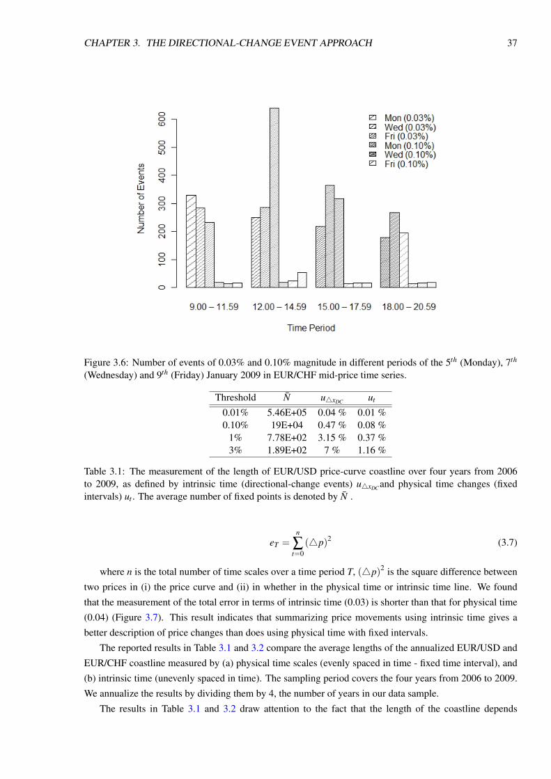
CHAPTER 3. THE DIRECTIONAL-CHANGE EVENT APPROACH 37
Figure 3.6: Number of events of 0.03% and 0.10% magnitude in different periods of the 5th (Monday), 7th
(Wednesday) and 9th (Friday) January 2009 in EUR/CHF mid-price time series.
Threshold N̄ u4xDC ut
0.01% 5.46E+05 0.04 % 0.01 %0.10% 19E+04 0.47 % 0.08 %
1% 7.78E+02 3.15 % 0.37 %3% 1.89E+02 7 % 1.16 %
Table 3.1: The measurement of the length of EUR/USD price-curve coastline over four years from 2006to 2009, as defined by intrinsic time (directional-change events) u4xDC and physical time changes (fixedintervals) ut . The average number of fixed points is denoted by N̄ .
eT =n
∑t=0
(4p)2 (3.7)
where n is the total number of time scales over a time period T, (4p)2 is the square difference between
two prices in (i) the price curve and (ii) in whether in the physical time or intrinsic time line. We found
that the measurement of the total error in terms of intrinsic time (0.03) is shorter than that for physical time
(0.04) (Figure 3.7). This result indicates that summarizing price movements using intrinsic time gives a
better description of price changes than does using physical time with fixed intervals.
The reported results in Table 3.1 and 3.2 compare the average lengths of the annualized EUR/USD and
EUR/CHF coastline measured by (a) physical time scales (evenly spaced in time - fixed time interval), and
(b) intrinsic time (unevenly spaced in time). The sampling period covers the four years from 2006 to 2009.
We annualize the results by dividing them by 4, the number of years in our data sample.
The results in Table 3.1 and 3.2 draw attention to the fact that the length of the coastline depends

CHAPTER 3. THE DIRECTIONAL-CHANGE EVENT APPROACH 38
Figure 3.7: EUR/USD mid-prices time series defined by physical time and intrinsic time. The samplingperiod is over November 5th, 2009. For intrinsic time, the number of events is 30 determined by a thresholdsize of 0.1%.
completely on the frequency of changes in the price. Also, these reported results highlight the importance of
considering events in studying the price-curve, rather than physical time changes due to the long coastline
of price changes based on intrinsic time. In all the thresholds that we have tested, the length of the price-
curve coastline defined by physical time is shorter than the coastline defined by intrinsic time. Intrinsic time
enables the analyst to capture the short term market dynamics involved by presenting significant information
and a clear picture of price behaviour, based on the observer’s expectations of the market. In addition, it
reduces the complexity of real-world price time series given the small number of price points for evaluation.
The computational costs (which include the cost of evaluating data) must not be ignored. Thus, it should be
part of the criteria when it comes to deciding on an approach for studying price time series.
Threshold N̄ u4xDC ut
0.01% 6.99E+05 0.04 % 0.01 %0.10% 7.20E+03 0.56 % 0.07 %
1% 4.10E+02 3.11 % 0.29 %3% 3.00E+01 5.87 % 1.12 %
Table 3.2: The measurement of the length of EUR/CHF price-curve coastline over four years from 2006to 2009, as defined by intrinsic time (directional-change events) u4xDC and physical time changes (fixedintervals) ut . The average number of fixed points is denoted by N̄ .
CHAPTER 3. THE DIRECTIONAL-CHANGE EVENT APPROACH 39
3.6 ZI-DCT0
We would like to investigate whether the concept of directional-change event can be incorporated into a
trading strategy. We define a simple directional-change event trading strategy as one in which a trader will
commit itself to a fixed threshold. Whenever a trader detects an upturn DC event (according to the used
threshold), it will conclude that the market is on an upward run. This could mean an opportunity to buy.
Similarly, a downturn DC event indicates an opportunity to sell. We shall call this strategy a zero-intelligence
directional-change event trading strategy, or ZI-DCT0 for short. A trader that uses ZI-DCT0 will be referred
to as a ZI-DCT0 trader.
Incorporating the directional-change event approach to the traders’ trading strategy will reduce the com-
plexity of the time series of prices. Accordingly traders can capture the short term market dynamics involved
based on their expectations of the market towards an obvious representation of the market dynamic, and,
based on that, it will allow them to detect fewer major periodic stable patterns in a financial time series based
on their expectations of the market. Cautiousness in choosing a suitable threshold is essential to reflect the
real dynamic of the market involved, given that, when a threshold which is either too large or too small is
used, traders will often fail to spot many important patterns on the time series of prices.
3.6.1 Experiment
Experiments were conducted with the aim of studying the impact of ZI-DCT0 on a trader’s performance.
The experiment used daily closing historical prices for six stock indexes: FTSE100 stock index (16/04/2004
to 20/03/2008), SnP500 (26/03/2004 to 20/03/2008), DAX (19/04/2004 to 20/03/2008), Nasdaq (12/04/2004
to 20/03/2008), HangSeng (19/03/2004 to 20/03/2008) and Nikkei (20/02/2004 to 20/03/2008). In addition,
one of the experiments was conducted on randomly generated prices. The data records contain the daily
closing trade price data and each record is time stamped.
We proceed on the assumption that the ZI-DCT0 trader will trade on each stock index based on the
change in the daily closing historical prices over the whole period. Before the experiment begins, the ZI-
DCT0 trader is endowed with 1,000,000 amounts of cash and without any shares. The ZI-DCT0 trader
invests 100% of it cash when buying, and 100% of it shares when selling. The trader’s position on each
of the assets changes over time, as a result of the trader’s decision to buy or sell a specific quantity of the
asset. We used a variety of thresholds to demonstrate the role that the threshold has on the trader’s wealth
distribution.
3.6.2 Results
Table 3.3 presents the potential profits of ZI-DCT0 using different thresholds. These potential profits are the
returns of the trades made by a ZI-DCT0 trader evaluated throughout the complete test period as explained
in section 3.6.1. Several test runs are reported, giving estimates of the effectiveness and significance of the
ZI-DCT0 strategy.
From the results reported in Table 3.3, we see that the threshold plays a critical role in the trader’s
performance and we can see the big impact of each threshold value on the trading return. Speaking broadly,
for the majority of trading returns, the trader made more profits than losses based on the different thresholds
they used. This indicates that the returns are significant but also reminds us of the importance of fitting an
appropriate threshold to an appropriate asset.
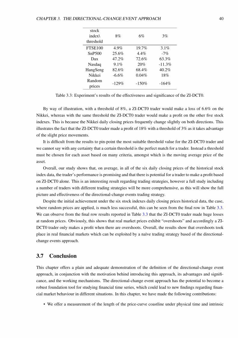
CHAPTER 3. THE DIRECTIONAL-CHANGE EVENT APPROACH 40
stockindex\
threshold8% 6% 3%
FTSE100 4.9% 19.7% 3.1%SnP500 25.6% 4.4% -7%
Dax 47.2% 72.6% 63.3%Nasdaq 9.1% 20% -11.3%
HangSeng 82.6% 68.4% 40.2%Nikkei -6.6% 0.04% 18%
Randomprices
-129% -150% -164%
Table 3.3: Experiment’s results of the effectiveness and significance of the ZI-DCT0.
By way of illustration, with a threshold of 8%, a ZI-DCT0 trader would make a loss of 6.6% on the
Nikkei, whereas with the same threshold the ZI-DCT0 trader would make a profit on the other five stock
indexes. This is because the Nikkei daily closing prices frequently change slightly on both directions. This
illustrates the fact that the ZI-DCT0 trader made a profit of 18% with a threshold of 3% as it takes advantage
of the slight price movements.
It is difficult from the results to pin-point the most suitable threshold value for the ZI-DCT0 trader and
we cannot say with any certainty that a certain threshold is the perfect match for a trader. Instead a threshold
must be chosen for each asset based on many criteria, amongst which is the moving average price of the
asset.
Overall, our study shows that, on average, in all of the six daily closing prices of the historical stock
index data, the trader’s performance is promising and that there is potential for a trader to make a profit based
on ZI-DCT0 alone. This is an interesting result regarding trading strategies, however a full study including
a number of traders with different trading strategies will be more comprehensive, as this will show the full
picture and effectiveness of the directional-change events trading strategy.
Despite the initial achievement under the six stock indexes daily closing prices historical data, the case,
where random prices are applied, is much less successful, this can be seen from the final row in Table 3.3.
We can observe from the final row results reported in Table 3.3 that the ZI-DCT0 trader made huge losses
at random prices. Obviously, this shows that real market prices exhibit “overshoots” and accordingly a ZI-
DCT0 trader only makes a profit when there are overshoots. Overall, the results show that overshoots took
place in real financial markets which can be exploited by a naïve trading strategy based of the directional-
change events approach.
3.7 Conclusion
This chapter offers a plain and adequate demonstration of the definition of the directional-change event
approach, in conjunction with the motivation behind introducing this approach, its advantages and signifi-
cance, and the working mechanisms. The directional-change event approach has the potential to become a
robust foundation tool for studying financial time series, which could lead to new findings regarding finan-
cial market behaviour in different situations. In this chapter, we have made the following contributions:
• We offer a measurement of the length of the price-curve coastline under physical time and intrinsic

CHAPTER 3. THE DIRECTIONAL-CHANGE EVENT APPROACH 41
time which represents the profit potential. The measurement shows a long coastline of price changes
defined by intrinsic time, confirming similar results in Glattfelder et al.’s [98] study. The aim of the
measurement of the length of the price-curve coastline reported in this chapter is to compare its length
measured under both intrinsic and physical time, which has not been explored by the Glattfelder et al.
[98] study. In addition to this, in this chapter we also measured the total error of the length of the price
curve coastline under both intrinsic and physical time, which shows that studying the price movements
using intrinsic time gives an improved description of price changes than does using physical time with
fixed intervals. Once again, this was not presented or mentioned in the Glattfelder et al. [98] study.
• We constructed a new trading strategy based on the directional-change event approach. This trading
strategy is called zero-intelligence directional-change event trading strategy or ZI-DCT0 for short.
ZI-DCT0 would allow traders to capture the short term market dynamics involved in the detection of
major periodic fixed patterns in price time series. Experiments were conducted using daily closing
historical prices for six stock indexes. These show the impact of ZI-DCT0 on a trader’s trading
performance.
In chapter 5, using the directional-change event approach, we study the EUR/USD and EUR/CHF price
time series, and discover four new scaling laws and six established quantitative relationships amongst them,
which hold across EUR/USD and EUR/CHF transactions. In chapter 6, we use the ZI-DCT0 strategy to
model two groups of agents in the market: trend-following and contrarian agents.

Chapter 4
Filtering of a High-Frequency FXTransactions Dataset
4.1 Introduction
High-frequency data (HFD) in finance represent a very large amount of data which is the full record of
transactions and their linked characteristics at frequencies higher than on a daily basis [63, 74]. The fact
that the FX market is the largest and most liquid financial market in the world makes it an important source
of HFD [63]. HFD play an important role in understanding financial market behaviour as they encapsulate
a plethora of information [63].
Although the rapid advances in computing and database technologies have made HFD available, nu-
merous challenges arise with regard to HFD processing and analysis. HFD have no standard structure,
since their structure is based on the policy and procedures of the institution that generates the data [44].
Unfortunately, HFD may incorporate some spurious data, erroneous data or may include some data gaps.
Such data may possibly result from computer system errors or the institution’s internal system procedures
[36, 44, 63]. Failure to identify erroneous data in the HFD could possibly have a significant effect on the
validity of the HFD analysis. Therefore, prior to studying and analysing HFD, a filtering process for the
HFD is an essential first step.
In the literature, there are some notable works dealing with the subject of HFD filtering [39, 44, 63, 182].
Each of these works adopts a different approach because of the different structure and types of erroneous
data of HFD being filtered. Consequently, the HFD filtering process is not standardized. Before undertaking
the filtering of the data, one needs to have an understanding of their nature and structure as well as the
purpose of their use. This will enable to explore and determine the types of erroneous data, and define the
detailed process of filtering, and finally to validate the consistency of the filtered dataset.
In this chapter 1, we present the filtering process associated with the HFD of individual traders’ historical
transactions on the OANDA FX trading platform. The aim of the filtering process is to remove any possible
erroneous data in terms of the traders’ actual transactions. The initial phase of the filtering process that we
conducted relies on two major steps: exploring and understanding the nature and structure of the data, and
1The work presented in this chapter has been taken in parallel by myself and Shaimaa Masry, a PhD student at the Centre forComputational Finance and Economic Agents at the University of Essex. Although we worked in parallel, we adopted differentmethodologies and accordingly developed different code. Fortunately, our results for the filtered dataset are very similar, whichindicates that both of us successfully eliminated the correct outliers from the dataset. Furthermore, such similarity of resultsconfirms the validity of the filtered dataset.
42

CHAPTER 4. FILTERING OF A HIGH-FREQUENCY FX TRANSACTIONS DATASET 43
studying OANDA’s internal system procedures since this might possibly affect the consistency of the data.
As a result of the filtering process, the number of transactions in the dataset was reduced to a total of ~ 59
million transactions from ~147 million transactions. By validating the filtered dataset, we confirmed the
consistency and reliability of the dataset.
The organization of this chapter is as follows. Section 4.2 provides an overview of the underlying dataset
and its potential usefulness. Section 4.3 presents a general overview of the outliers. Section 4.4 describes
the filtering process in conjunction with the results of the process. Section 4.5 provides the validation of the
filtered dataset. Section 4.6 states the behaviour and effects of the filtered dataset.
4.2 Overview of the Dataset
The HFD used in this study were provided by OANDA Corporation - short for Olsen And Associates. The
OANDA Corporation is a financial services provider for currency information and is an internet-based FX
market-maker for the trading of foreign currencies. The OANDA Corporation provides access to one of
the largest existing historical high-frequency datasets of currency exchange rates and transactions. OANDA
serves a diversity of traders, from individual traders to large corporations and financial institutions. In
OANDA, traders trade under the same terms and conditions, particularly under the same prices, with com-
petitive spreads. It is worth highlighting that in terms of FX trading platforms, only OANDA stores the
details of the traders’ historical transactions and their position history over a long time horizon, representing
the worldwide exposure of traders in the FX markets.
The high-frequency dataset used in this study represents OANDA’s individual traders’ historical trans-
actions at an account level made available on an anonymous basis and spanning 2.25 years, from 1st January
2007 to 5th March 2009. The dataset contains ~147 million historical transactions carried out by 45,845
different accounts trading in 48 different currency pairs under the same terms and conditions. The high-
frequency dataset of individual traders’ historical transactions is unique. Thus, the analysis of such a dataset
is extremely valuable, and significant in improving our understanding of FX market behaviour, and also
for building agent-based models of FX market traders. The dataset contains different accounts representing
individual traders, banks, central banks, hedge funds and others. Due to the detailed level of information
and the long time horizon of the dataset, the dataset is rich in terms of observations and interesting patterns.
Each historical transaction contains the following information: the account Id, the transaction Id, the
transaction timestamp, the traded currency pair, the execution price, the number of units traded, the amount
of units traded, and the transaction type. Figure 4.1 provides a snapshot of the high-frequency dataset of
individual traders’ historical transactions. A transaction is defined as an individual executed trade performed
on behalf of a trader’s account. The transaction Id is a unique identity for the executed transaction. Each
account in the OANDA FX trading platform has a unique account Id. It is important to highlight that every
account Id in the dataset has been changed by OANDA Corporation to protect the traders’ identity and
privacy. In addition, it is important to note that one individual trader may have more than one account. The
transaction timestamp is the execution time of the transaction. The transaction timestamp is stored in a Unix
time format. The traded currency pair of a transaction is represented as a base and a quote (base/quote)
e.g. EUR/USD. The amount of a single transaction is equal to the execution price times the number of units
traded, converted to the account’s home currency.
A transaction can be one of the following six types: BuyMarket, SellMarket, CloseTradeB, Close-

CHAPTER 4. FILTERING OF A HIGH-FREQUENCY FX TRANSACTIONS DATASET 44
Figure 4.1: Snapshot of a sample from the high-frequency dataset of individual traders’ historical transac-tions.
TradeS, ClosePositionB or ClosePositionS. A BuyMarket is a transaction to buy a number of units of the
base currency and sell an equal amount of units of the quoted currency to pay for the base currency. A
SellMarket is a transaction to sell a number of units of the base currency and buy an equal amount of the
quoted currency to buy the base currency. Active transactions are called open positions. An open position
is closed by placing a transaction that has an equal amount and takes the opposite type to the open position.
It is possible to increase or decrease an open position’s size. Based on OANDA’s internal system storage
procedures, a single transaction of the type BuyMarket or SellMarket, is recorded in the database as more
than one transaction in the event of a closing previous sell or buy orders placed by the trader. A transaction
of type CloseTradeB closes a single previous transaction of type BuyMarket, while a transaction of type
CloseTradeS closes a single previous transaction of type SellMarket. A transaction of type ClosePositionB
closes a single or a sequence of transactions of type BuyMarket in a certain currency pair. Similarly, a trans-
action of type ClosePositionS closes a single or a sequence of transactions of type SellMarket in a certain
currency pair. Based on OANDA’s internal system storage procedures, transactions of type ClosePositionB
(ClosePositionS) are recorded in the database as more than one transaction in the event of closing more
than one transaction of type BuyMarket (SellMarket) in which each transaction of type ClosePositionB
(ClosePositionS) has a number of traded units equivalent to the units of each open BuyMarket (SellMarket)
order.
4.3 Outliers
Some of the transactions in the dataset may possibly be erroneous transaction data. To test such a hypothesis,
we select five accounts from the dataset at random and aggregate the number of transactions of the accounts
over minute bases (depicted in Figure 4.2). From Figure 4.2, we can see that some possible outliers occur at
different time points in terms of the account’s transaction activities. An outlier is defined as transaction data
that were not placed by an account, and therefore is an incorrectly reported transaction which is identified as
a data error. Such outliers raise an important critical question: do these outliers possibly indicate transactions
data that are incorrectly reported, or are these outliers the result of the sudden change in the account’s trading
behaviour? A failure to identify these outliers as erroneous transactions data will significantly affect the
validity of the analysis. For that reason, it is necessary to filter the dataset to identify any possible erroneous
transactions which do not correspond to the traders’ trading activity.
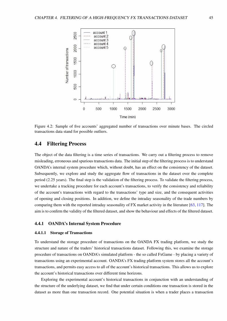
CHAPTER 4. FILTERING OF A HIGH-FREQUENCY FX TRANSACTIONS DATASET 45
Figure 4.2: Sample of five accounts’ aggregated number of transactions over minute bases. The circledtransactions data stand for possible outliers.
4.4 Filtering Process
The object of the data filtering is a time series of transactions. We carry out a filtering process to remove
misleading, erroneous and spurious transactions data. The initial step of the filtering process is to understand
OANDA’s internal system procedure which, without doubt, has an effect on the consistency of the dataset.
Subsequently, we explore and study the aggregate flow of transactions in the dataset over the complete
period (2.25 years). The final step is the validation of the filtering process. To validate the filtering process,
we undertake a tracking procedure for each account’s transactions, to verify the consistency and reliability
of the account’s transactions with regard to the transactions’ type and size, and the consequent activities
of opening and closing positions. In addition, we define the intraday seasonality of the trade numbers by
comparing them with the reported intraday seasonality of FX market activity in the literature [63, 117]. The
aim is to confirm the validity of the filtered dataset, and show the behaviour and effects of the filtered dataset.
4.4.1 OANDA’s Internal System Procedure
4.4.1.1 Storage of Transactions
To understand the storage procedure of transactions on the OANDA FX trading platform, we study the
structure and nature of the traders’ historical transactions dataset. Following this, we examine the storage
procedure of transactions on OANDA’s simulated platform - the so called FxGame - by placing a variety of
transactions using an experimental account. OANDA’s FX trading platform system stores all the account’s
transactions, and permits easy access to all of the account’s historical transactions. This allows us to explore
the account’s historical transactions over different time horizons.
Exploring the experimental account’s historical transactions in conjunction with an understanding of
the structure of the underlying dataset, we find that under certain conditions one transaction is stored in the
dataset as more than one transaction record. One potential situation is when a trader places a transaction

CHAPTER 4. FILTERING OF A HIGH-FREQUENCY FX TRANSACTIONS DATASET 46
of type BuyMarket, SellMarket, ClosePositionB or ClosePositionS that closes previously open sell or buy
orders. Another potential situation is a transaction which takes place as a result of a profit taking limit order
or a stop loss limit order. A profit taking limit order is an order to close an open position once the price
movement has reached a profit threshold. In contrast, a stop loss limit order is an order to close an open
position once the price movement hits a loss threshold. A further potential situation is if a transaction takes
place as a result of a margin call. A margin call is a procedure on the part of the market-maker executing
the transaction to close out an account’s open positions once the account’s balance has cascaded under the
minimum margin required to cover the size of the account’s currently open positions.
Hence, if we were to study and analyse the traders’ historical transactions in the current state of the
dataset, we would probably get ambiguous information regarding the traders’ moves and trading activity
because the dataset contains erroneous data. Thus, we conduct a merging procedure on groups of associated
transactions. These groups of associated transactions can be categorized as follows:
1. The first group includes a sequence of associated transactions which have identical data with regard
to the following: same account Id, same currency pair, same timestamp, same execution price and
same type of transaction. Figure 4.3 shows a sample from the dataset of individual traders’ historical
transactions which represents an example of the first group of associated transactions. This group
of associated transactions is merged into one transaction in which the traded units and amounts are
aggregated.
2. The second group is limited to transactions of types ClosePositionB and ClosePositionS. The features
of the second group are similar to the first group. However, some of the associated transactions in
the second group have different timestamps with a few seconds difference. To identify whether a set
of associated transactions having different timestamps is the result of one trade, we check whether or
not the trader has placed a new transaction of type BuyMarket or SellMarket for the same currency
pair as those for the set of associated transactions in the time period between the set of associated
transactions. If no such transaction is recorded in the dataset, the set of associated transactions is
merged. In detail, the traded units and the amounts in this set of transactions are aggregated, and the
average of the transactions’ timestamps is recorded for the merged transaction. Figure 4.4 shows a
sample from the dataset of individual traders’ historical transactions which represents an example of
the second group of associated transactions.
3. The third group includes a sequence of associated transactions which have identical data with regard
to the following: same account Id, same currency pair, same timestamp and same type of transaction.
However, some of these associated transactions have different execution prices. The transactions in
the third group are either of type BuyMarket or SellMarket. Figure 4.5 shows a sample from the
dataset of individual traders’ historical transactions which represents an example of the third group
of associated transactions. Although these associated transactions may possibly be the results of one
trade, we came to a decision not to merge them. The problem of merging them would be defining an
average price for the trade, but this modification in the execution price could result in information loss
in terms of actual execution prices, and consequently the transaction’s profitability.
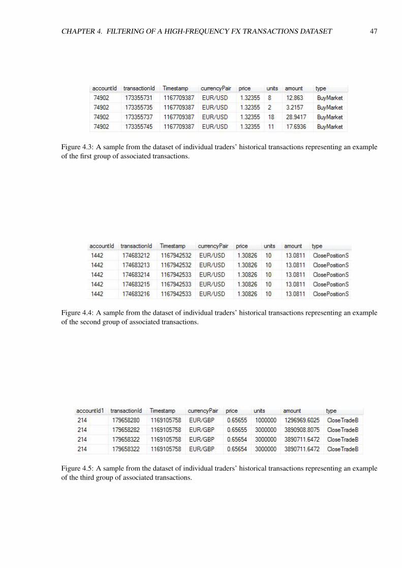
CHAPTER 4. FILTERING OF A HIGH-FREQUENCY FX TRANSACTIONS DATASET 47
Figure 4.3: A sample from the dataset of individual traders’ historical transactions representing an exampleof the first group of associated transactions.
Figure 4.4: A sample from the dataset of individual traders’ historical transactions representing an exampleof the second group of associated transactions.
Figure 4.5: A sample from the dataset of individual traders’ historical transactions representing an exampleof the third group of associated transactions.

CHAPTER 4. FILTERING OF A HIGH-FREQUENCY FX TRANSACTIONS DATASET 48
Figure 4.6: Spurious transactions encompass a traded amount value of zero indicating that interest paymentshave been incurred.
Figure 4.7: The total number of transactions for each month in the dataset (a) before and (b) after the filteringprocess respectively against the (c) total number of accounts.
4.4.1.2 Interest Payment Procedure
The system in the OANDA FX trading platform implies a continuous series of second-by-second interest
payments on each account’s open position. This is in contrast to some of the FX market-maker’s trading
platforms in which interest payment is computed just once a day on each account’s open position. The
dataset of individual traders’ historical transactions does not include detailed information regarding the
computed interest payments. Nevertheless, OANDA’s interest payments’ procedure records spurious trans-
actions which encompass a traded amount value of zero indicating that interest payments have been incurred
(as shown in Figure 4.6). Such spurious transactions are removed from the dataset of individual traders’ his-
torical transactions. The existence of these spurious transactions in the dataset would otherwise affect the
validity of the analysis.
4.4.2 Flow of Transactions
Figure 4.7 shows the total number of transactions for each month in the dataset, before and after the filtering
process respectively, against the total number of accounts in the dataset. Despite the fact that the filtered
dataset does not contain spurious transactions, or even unmerged transactions corresponding to one real
transaction, we can note the high number of transactions during 2007 compared to 2008, and sudden drops
in the numbers of transactions following August 2007. An important observation which has to be explained
is the increase in the total number of transactions in August 2007, followed by a sudden drop in September
2007, combined with an increase in the total number of accounts in October 2007 and throughout 2008. The
drop in the total number of transactions and accounts over March 2009 are a data artefact, and accordingly
must be ignored, given that there were just five days in March 2009.
It is essential to explore and understand the flow of the total number of transactions for each month in

CHAPTER 4. FILTERING OF A HIGH-FREQUENCY FX TRANSACTIONS DATASET 49
Figure 4.8: The number of high-frequency accounts in each month in the dataset.
Figure 4.9: Correlation between the total numbers of daily transactions placed by high-frequency (HF)accounts, and the total numbers of transactions in each month.
the dataset respectively, against the flow of the total number of accounts for each month. This will allow
us to understand whether the sudden increase in the total number of transactions in August 2007 is due to
traders increasing their trading frequency, or whether it is due to spurious transactions. Hence, we examine
the trading frequency for all the accounts in the dataset over the whole period. The trading frequency is
defined as the maximum number of transactions placed by each account in one day for each month.
We find that the daily maximum number of transactions for an account vary from one transaction to
thousands of transactions. We define an account as a high-frequency account when the account has more
than 1,000 transactions for at least one day in a month. The trading frequency of a high-frequency account
can vary over the days. We find 114 high-frequency accounts in the dataset. Figure 4.8 shows the number
of high-frequency active accounts in each month in the dataset. From Figure 4.8, we can observe a high
number of high-frequency accounts in 2007 compared to the remaining dataset time period. By relating the
total numbers of daily transactions placed by high-frequency accounts to the total numbers of transactions
in each month, we find a strong positive correlation between them (Figure 4.9). The strength of this strong
positive correlation is reflected in a correlation coefficient of +0.90. Such a strong positive correlation
indicates that the increase in the number of transactions in 2007 is a result of the large number of transactions
placed by the high-frequency accounts.
We find that 48.33% of the transactions in the dataset are placed by the high-frequency accounts. How-

CHAPTER 4. FILTERING OF A HIGH-FREQUENCY FX TRANSACTIONS DATASET 50
Figure 4.10: Example of the filtered dataset validation results produced by tracking a sample of a sequenceof EUR/USD transactions for a sample account.
ever, an extraordinary and ambiguous feature is that the total trading volumes of the high-frequency accounts
represents merely 0.69 % of the total trading volumes in the dataset. The trading volume is defined as the to-
tal traded units in the dataset. Having an exceptionally small trading volume (0.69%) relative to the number
of transactions (48.33%), the identified high-frequency accounts may possibly be spurious accounts. These
spurious accounts may possibly be part of OANDA’s FX trading platform for testing purposes. For that
reason, we remove the 114 high-frequency accounts, and consequently their transactions.
4.4.3 Results
The output of the filtering process results in a reduction of 70.73% of the transactions from the dataset of the
individual traders’ historical transactions. The total number of transactions in the dataset before the filtering
process was ~ 147 million transactions while after the filtering process the total number of transactions was
reduced to ~ 59 million transactions.
4.5 Validation
Subsequent to filtering a high-frequency dataset, a validation procedure has to be conducted to validate the
reliability and consistency of the filtered dataset. In our study, the validation procedure implies tracking for
each of the account’s traded currency pairs, each transaction’s traded units bought and sold in sequence in
terms of the transactions’ execution time. The validation procedure traces different types of transactions of
each account with reference to a given currency pair, from the opening to the closing of a position. Figure
4.10 offers a straightforward example of the results produced by tracking a sample of sequence EUR/USD
transactions for a sample account. The exposure refers to an account’s total holdings of a traded currency
pair. The exposure is defined as the net sum of the traded units of an opened position transactions. A traded
units are signed in terms of the transaction type. The traded units are represented by a positive sign when
the transaction type is BuyMarket, and negative when the transaction type is SellMarket. The exposure
is signed in terms of the position type. A positive exposure refers to a long position, whereas a negative
exposure refers to a short position.
The results of the validation procedure confirm the reliability and consistency of the filtered dataset of
individual traders’ historical transactions in the OANDA FX trading platform. Whatever the causes behind
the existence of possible misleading and spurious data in the underlying dataset, the filtering process has
successfully eliminated those misleading and spurious data, resulting in a consistent dataset.
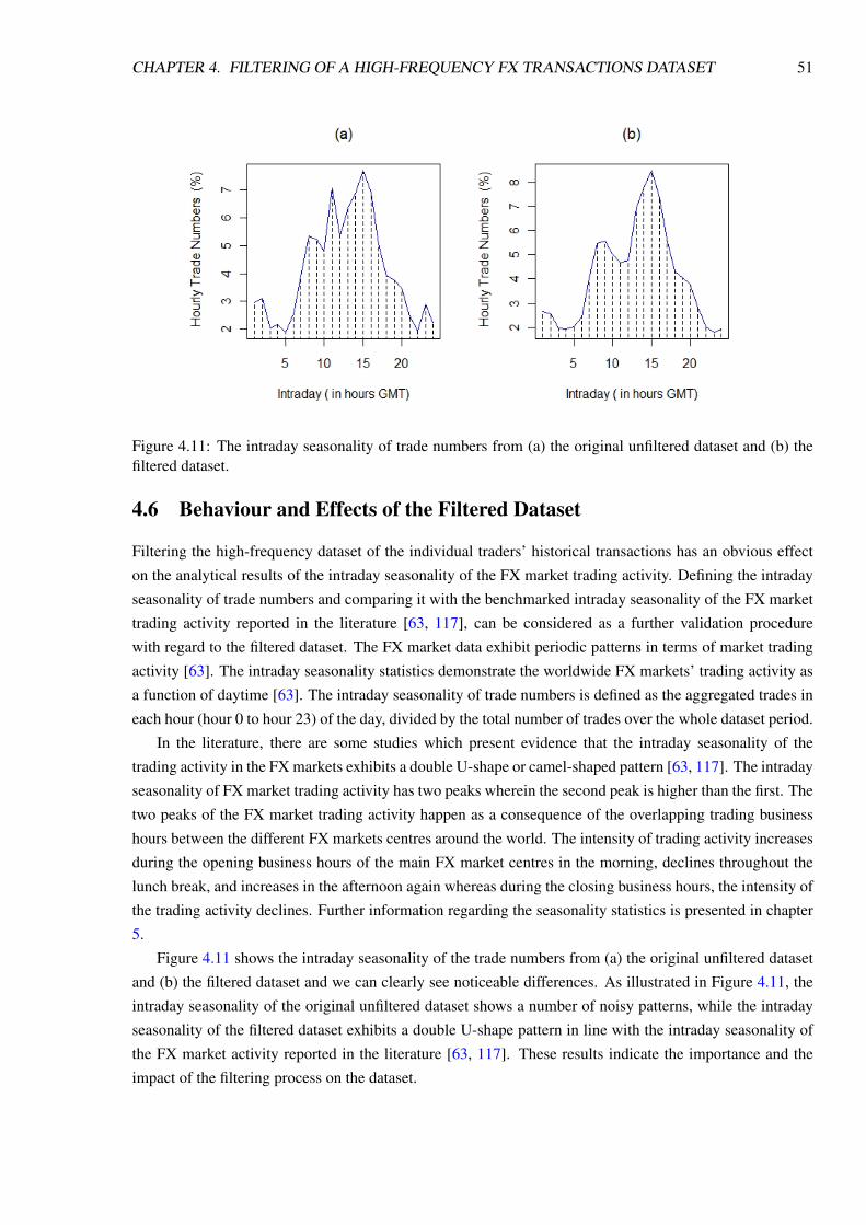
CHAPTER 4. FILTERING OF A HIGH-FREQUENCY FX TRANSACTIONS DATASET 51
Figure 4.11: The intraday seasonality of trade numbers from (a) the original unfiltered dataset and (b) thefiltered dataset.
4.6 Behaviour and Effects of the Filtered Dataset
Filtering the high-frequency dataset of the individual traders’ historical transactions has an obvious effect
on the analytical results of the intraday seasonality of the FX market trading activity. Defining the intraday
seasonality of trade numbers and comparing it with the benchmarked intraday seasonality of the FX market
trading activity reported in the literature [63, 117], can be considered as a further validation procedure
with regard to the filtered dataset. The FX market data exhibit periodic patterns in terms of market trading
activity [63]. The intraday seasonality statistics demonstrate the worldwide FX markets’ trading activity as
a function of daytime [63]. The intraday seasonality of trade numbers is defined as the aggregated trades in
each hour (hour 0 to hour 23) of the day, divided by the total number of trades over the whole dataset period.
In the literature, there are some studies which present evidence that the intraday seasonality of the
trading activity in the FX markets exhibits a double U-shape or camel-shaped pattern [63, 117]. The intraday
seasonality of FX market trading activity has two peaks wherein the second peak is higher than the first. The
two peaks of the FX market trading activity happen as a consequence of the overlapping trading business
hours between the different FX markets centres around the world. The intensity of trading activity increases
during the opening business hours of the main FX market centres in the morning, declines throughout the
lunch break, and increases in the afternoon again whereas during the closing business hours, the intensity of
the trading activity declines. Further information regarding the seasonality statistics is presented in chapter
5.
Figure 4.11 shows the intraday seasonality of the trade numbers from (a) the original unfiltered dataset
and (b) the filtered dataset and we can clearly see noticeable differences. As illustrated in Figure 4.11, the
intraday seasonality of the original unfiltered dataset shows a number of noisy patterns, while the intraday
seasonality of the filtered dataset exhibits a double U-shape pattern in line with the intraday seasonality of
the FX market activity reported in the literature [63, 117]. These results indicate the importance and the
impact of the filtering process on the dataset.
CHAPTER 4. FILTERING OF A HIGH-FREQUENCY FX TRANSACTIONS DATASET 52
4.7 Conclusion
In this chapter, we have filtered a unique high-frequency dataset of individual traders’ historical transactions
consisting of over 40,000 anonymous accounts on the OANDA FX trading platform. The underlying feature
of the filtering process is to identify and eliminate any potential misleading or spurious data which may
possibly affect the validity of the analysis and the subsequent results. This chapter makes the following
contributions to the literature:
• We have conducted a customized filtering procedure to remove potentially misleading and spurious
transactions from the individual traders’ historical transactions dataset. We have found misleading
transactions in the dataset resulting from OANDA’s internal system storage procedure (as explained
in section 4.4.1.1). In addition, we have found spurious transactions in the dataset results with regard
to (a) OANDA’s interest payment procedure (as explained in section 4.4.1.2) and (b) the existence of
spurious accounts (as explained in section 4.4.2).
• We have validated the reliability and consistency of the filtered dataset.
• We have demonstrated the behaviour and effects of the filtered dataset in the exhibition of the intraday
seasonality of the FX market trading activity (demonstrated in section 4.6). Such a demonstration
confirms the importance and the impact of the filtering process on the validity of the analysis of
high-frequency datasets.
In the next chapter, we analyse and study the filtered high-frequency dataset of individual traders’ historical
transactions in the OANDA FX trading platform. The aim is to establish a set of stylized facts which
characterize the traders’ collective behaviour in the FX market in order to provide a benchmark for validating
agent-based models of the FX market.

Chapter 5
Stylized Facts of Trading Activity in the FXMarket
5.1 Introduction
Financial markets are active and dynamic environments generating increasingly large volumes of data at
frequencies higher than on a daily basis. Such data have been the focus of study by both the academic
community and industry analysts from a number of perspectives. One key area in the study of financial
markets data is the establishment of their statistical properties [104]. These statistical properties are known
as stylized facts, and are established from the statistical analysis of data [57]. Stylized facts can provide
useful insights into the workings of the real market, the behaviour of individual traders, the forces that drive
behaviour, and their impact on the market dynamics. Establishing stylized facts with regard to the behaviour
of traders and their trading activities is an important step in modelling financial markets [63]. In building
models of financial markets, stylized facts can be used as verification criteria [137] to confirm that an ABM
is indeed a model of the real market if it is able to reproduce the stylized facts to a satisfactory extent. A
number of studies have established the stylized facts associated with price returns [57, 63, 104], order books
[75, 77] and trading activity [63, 117] in the market.
To establish the stylized facts of FX market traders’ behaviour, we need to explore the high-frequency
data (HFD) of their historical trading activities in the market. HFD allows us to explore some of the prop-
erties of trading behaviour that cannot be observed at lower frequencies (e.g. daily data) [63]. Despite the
availability of studies establishing the stylized facts of price returns and order flow in the financial markets,
the establishment of the stylized facts relating to trading activity in the high-frequency FX market is still in
its infancy [63]. Dacorogna et al. [63] established some basic stylized facts with regard to the seasonality
of trading activity in the FX markets by quantifying the trade frequency and volume using price tick data.
They show that the intraday dynamics of trading activity in the FX market exhibits a double U-shape or
camel-shape pattern. Ito and Hashimoto [117] established basic stylized facts associated with seasonality
and correlation behaviour for the USD/YEN and the EUR/USD. Their work confirmed the existence of the
U-shape pattern of intraday activities for Tokyo and London participants. They have also found that the
price changes and the trade volumes have a positive correlation.
In this chapter, we present a set of stylized facts that have been identified through the study of a HF
transactions dataset. Our study involves a unique HFD representing the physical transactions of anonymous
accounts from January 1, 2007 to March 5, 2009. The large size of the dataset and, most importantly, the
53

CHAPTER 5. STYLIZED FACTS OF TRADING ACTIVITY IN THE FX MARKET 54
level of detail of the dataset, allows for a microscopic analysis of the traders’ trading behaviour. In addition,
our study makes use of EUR/USD and EUR/CHF prices from January 1, 2007 to March 5, 2009. Our aim
is to establish stylized facts of the trading activity in the high-frequency FX market in order to gain insights
into the workings of the market, but also to establish a benchmark for validating FX market agent-based
models. We aim to confirm and extend the seasonality and correlation statistics work described in [63, 117].
Also, we aim to confirm and extend the scaling laws discovered in [98].
The organization of this chapter is as follows. The scaling laws are described in section 5.2, whereas
section 5.3 describes the intraday and intraweek seasonality. Section 5.4 describes the correlation behaviour
of the different FX market trading activity.
5.2 Scaling Laws
Scaling laws establish quantitative relationships between the size of price movements and the market ac-
tivity as a function of the time interval at which they are measured. Following Glattfelder et al.’s work
in [98], we have extended the set of stylized facts of the FX market by observing four new scaling laws,
next to establishing six quantitative relationships amongst them, holding across EUR/USD and EUR/CHF
transactions. Since prices in the market change at uneven time intervals, the measurement of market trading
activity needs to be adaptive beyond the notion of physical time scale changes. In this regard, our statistical
analysis depends on an event-driven approach – the so-called directional-change event approach. For details
regarding the directional-change event approach we refer the interested reader to chapter 3.
In this section, we consider 2.25 years of tick-by-tick data for EUR/USD and EUR/CHF prices over
January 1, 2007 to March 5, 2009. The data includes a bid and an ask price of a currency pair at a timestamp.
Throughout the chpater, the following definition of mid-price is used:
pm,t =(bt +at)
2(5.1)
where pm,t is the mid-price of a currency pair at time t, and bt and at are the bid and ask price respectively
at time t.
5.2.1 Empirical Evidence on Existing Stylized Facts
In this section, we have empirically confirmed from the existing literature four scaling laws and three quan-
titative relationships amongst them. These four scaling laws hold across EUR/USD and EUR/CHF prices.
Law (0a) is observed in a physical time scale whereas the other laws are observed in an intrinsic time scale
(directional-change event). The computation of laws (0b), (0c) and (0d) relies on the detection of DC and
OS events instead of focusing on the stochastic nature of the data-series.
The scaling law (0a) was discovered by Müller et al. in [174] and relates the size of the average absolute
mid-price change (return), sampled at time intervals ∆t, to the size of the time interval
〈|∆xt |〉=(
∆tCx
)Ex
(5.2)
where Cx and Ex are the scaling law parameters and a price move ∆xt at time t is defined as

CHAPTER 5. STYLIZED FACTS OF TRADING ACTIVITY IN THE FX MARKET 55
∆xt =(pm,t − pm,t−1)
pm,t−1(5.3)
The scaling laws parameters are the results of the line fit, where Ex is the slope and Cx is the intercept.
The slope measures the proportional change of the average absolute mid-price change due to an increment
in the time interval.
Using the directional-change event approach as explained in chapter 3, we define DC and OS events in
EUR/USD and EUR/CHF mid-price time series for a set of thresholds of different size, ranging from 0.10%
to 0.80%. We have confirmed the scaling law (0b) which was discovered by Guillaume et al. [104]. Law
(0b) relates the number N (∆xDC) of DC events to the size of the DC event ∆xDC
N (∆xDC) =
(∆xDC
CN,DC
)EN,DC
(5.4)
where CN,DC and EN,DC are the scaling law parameters.
The average results of the different event thresholds that we considered confirm the two scaling laws
discovered by Glattfelder et al. in [98]:
1. Law (0c) relates the time during which events occur to the size of these events. Given a fixed percent-
age threshold, the average time interval 〈∆tx〉 for a price move of size ∆x to occur is scale-invariant to
the size of the threshold
〈∆tx〉=(
∆xCt,x
)Et,x
(5.5)
where Ct,x and Et,x are the scaling law parameters.
2. Law (0d) counts the average number of ticks observed during every event. Given a fixed percentage
threshold, the average number of ticks 〈N (∆xtick)〉 observed during a price move of size ∆x is scale-
invariant to the size of this threshold
〈N (∆xtick)〉=(
∆xCN,tick
)EN,tick
(5.6)
where a tick is defined as an individual quote of bid and ask price by a market-maker, CN,tick and
EN,tick are the scaling law parameters.
The scaling law parameters are estimated using a standard linear regression. Laws (0b), (0c) and (0d) are
plotted in Figure 5.1. Table 5.1 reports the adjusted R2 values and the standard error of the fit.
The average obtained results (given in Figure 5.1) of the different event thresholds that we considered
confirm the three quantitative relationships among laws (0c) and (0d) which were discovered by Glattfelder
et al. in [98]:
1. A DC event of size ∆xDC is followed by one OS event of the same size
(〈∆xDC〉 ≈ 〈∆xOS〉) (5.7)
2. An OS event takes twice as long as a DC event to unfold
(〈|∆tOS|〉 ≈ 2〈|∆tDC|〉) (5.8)

CHAPTER 5. STYLIZED FACTS OF TRADING ACTIVITY IN THE FX MARKET 56
Figure 5.1: Scaling laws (a) 0b, (b) 0c and (c) 0d are plotted where the x-axis shows the price movesthresholds of the EUR/USD and EUR/CHF observations and the y-axis the (a) average number of events,the (b) average time (in seconds) and the (c) average tick numbers.
where 〈|∆tOS|〉 is the average time it takes an OS event to unfold while 〈|∆tDC|〉 is the average time it
takes a DC event to unfold.
3. An OS event contains twice as many ticks as a DC event
(〈N (∆xOS,tick)〉≈ 2〈N (∆xDC,tick)〉) (5.9)
where 〈N (∆xOS,tick)〉 and 〈N (∆xDC,tick)〉 are the average tick numbers in an OS and a DC event,
respectively.
EUR/USD EUR/CHFDC OS DC OS
Adj. R2 SE AAdj. R2 SE Adj. R2 SE Adj. R2 SEDirectional changes 0.99 0.35 - - 0.99 0.44 - -Time interval 0.99 0.34 0.99 0.22 0.99 0.04 0.99 0.05Tick numbers 0.99 0.36 0.99 0.35 0.99 0.43 0.99 0.45
Table 5.1: Estimated regression parameters: the adjusted R2 values of the fits, plus their standard errors(SE), for the scaling laws measured under DC and OS events. The sampling period covers 2.25 years from1st January 2007 to 5th March 2009.

CHAPTER 5. STYLIZED FACTS OF TRADING ACTIVITY IN THE FX MARKET 57
5.2.2 The New Scaling Laws
We have already mentioned in section 5.2.1 that the results of the empirical evidence indicate a scaling
behaviour observed in price data. Extending Glattfelder et al.’s work [98], we identified four new scaling
laws and cross-checked our results by establishing six quantitative relationships amongst them, holding
across EUR/USD and EUR/CHF transactions. It is important to highlight the fact that the first set of scaling
laws reported in section 5.2.1 applies to price data, while the second set of scaling laws reported in this
section applies to transactions data. A transaction represents an executable order in the market.
Scaling Law (1): Trade Numbers
Given a fixed percentage threshold, the average number of trades 〈N (∆xtrade)〉 observed during an event is
scale-invariant to the size of this threshold
〈N (∆xtrade)〉=(
∆xCN,trade
)EN,trade
(5.10)
where a trade is defined as an individual transaction, CN,trade and EN,trade are the scaling law parameters. In
essence, this law counts the average number of trades observed during every event. Law (1) is plotted in
Figure 5.2 and Table 5.2 reports the adjusted R2 values and the standard error of the fit. The results of Law
(1) show that on average, an OS event contains roughly twice as many trades as a DC event
〈N (∆xOS,trade)〉≈ 2〈N (∆xDC,trade)〉 (5.11)
where 〈N (∆xOS,trade)〉 and 〈N (∆xDC,trade)〉 are the average trade numbers in an OS and a DC event,
respectively.
Scaling Law (2): Trade Volumes
Given a fixed percentage threshold, the average volume of trades 〈V (∆xtrade)〉 observed during an event is
scale-invariant to the size of this threshold
〈V (∆xtrade)〉=(
∆xCV,trade
)EV,trade
(5.12)
where a trade volume for a single transaction i, denoted by Vi, is defined as the execution price times the
number of units of the transaction. CV,trade and EV,trade are the scaling law parameters. In detail, this law
counts the average volume of trades observed during every event. Law (2) is plotted in Figure 5.3. Table 5.2
reports the adjusted R2 values and the standard error of the fit. The results of the different event thresholds
that we considered show that on average, an OS event contains roughly twice as many volumes as a DC
event
〈V (∆xOS,trade)〉≈ 2〈V (∆xDC,trade)〉 (5.13)

CHAPTER 5. STYLIZED FACTS OF TRADING ACTIVITY IN THE FX MARKET 58
Figure 5.2: Average EUR/USD and EUR/CHF trade numbers during DC and OS events for selected thresh-old values. The x-axis shows the price moves thresholds of the EUR/USD and EUR/CHF observations andthe y-axis the average trade numbers.
where 〈V (∆xOS,trade)〉 and 〈V (∆xDC,trade)〉 are the average trading volumes in an OS and a DC event,
respectively.
Scaling Law (3): Number of Opening Positions
This law counts the average number of opening positions observed during every event of size ∆x. Given a
fixed percentage threshold, the average number of opening positions 〈N (∆xOP)〉 observed during an event
is scale-invariant to the size of this threshold
〈N (∆xOP)〉=(
∆xCN,OP
)EN,OP
(5.14)
where CN,OP and EN,OP are the scaling law parameters. Law (3) is plotted in Figure 5.4 and Table 5.2
reports the adjusted R2 values and the standard error of the fit.
Scaling Law (4): Number of Closing Positions
This law counts the average number of closing positions observed during every event. Given a fixed per-
centage threshold, the average number of closing positions 〈N (4xCP)〉 observed during an event is scale-
invariant to the size of this threshold
〈N (∆xCP)〉=(
∆xCN,CP
)EN,CP
(5.15)
where CN,CP and EN,CP are the scaling law parameters. Law (4) is plotted in Figure 5.5 and Table 5.2
reports the adjusted R2 values and the standard error of the fit. The average results of Laws (3) and (4) show
two important features:

CHAPTER 5. STYLIZED FACTS OF TRADING ACTIVITY IN THE FX MARKET 59
Figure 5.3: Average EUR/USD and EUR/CHF trade volumes during DC and OS events for selected thresh-old values. The x-axis shows the price moves thresholds of the EUR/USD and EUR/CHF observations andthe y-axis the average trade volumes.
Figure 5.4: Average number of opening EUR/USD and EUR/CHF positions observed during DC and OSevents for selected threshold values. The x-axis shows the price moves thresholds of the EUR/USD andEUR/CHF observations and the y-axis the average number of opening positions.
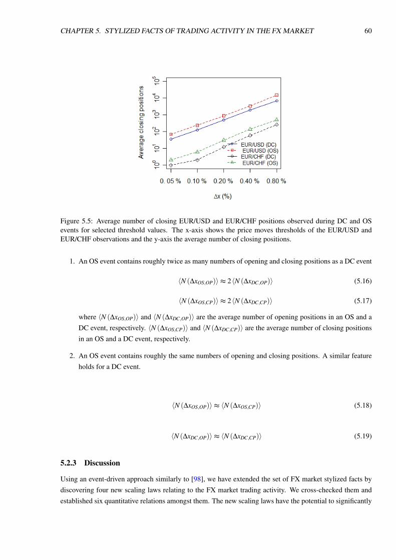
CHAPTER 5. STYLIZED FACTS OF TRADING ACTIVITY IN THE FX MARKET 60
Figure 5.5: Average number of closing EUR/USD and EUR/CHF positions observed during DC and OSevents for selected threshold values. The x-axis shows the price moves thresholds of the EUR/USD andEUR/CHF observations and the y-axis the average number of closing positions.
1. An OS event contains roughly twice as many numbers of opening and closing positions as a DC event
〈N (∆xOS,OP)〉≈ 2〈N (∆xDC,OP)〉 (5.16)
〈N (∆xOS,CP)〉≈ 2〈N (∆xDC,CP)〉 (5.17)
where 〈N (∆xOS,OP)〉 and 〈N (∆xDC,OP)〉 are the average number of opening positions in an OS and a
DC event, respectively. 〈N (∆xOS,CP)〉 and 〈N (∆xDC,CP)〉 are the average number of closing positions
in an OS and a DC event, respectively.
2. An OS event contains roughly the same numbers of opening and closing positions. A similar feature
holds for a DC event.
〈N (∆xOS,OP)〉≈ 〈N (∆xOS,CP)〉 (5.18)
〈N (∆xDC,OP)〉≈ 〈N (∆xDC,CP)〉 (5.19)
5.2.3 Discussion
Using an event-driven approach similarly to [98], we have extended the set of FX market stylized facts by
discovering four new scaling laws relating to the FX market trading activity. We cross-checked them and
established six quantitative relations amongst them. The new scaling laws have the potential to significantly

CHAPTER 5. STYLIZED FACTS OF TRADING ACTIVITY IN THE FX MARKET 61
EUR/USD EUR/CHFDC OS DC OS
Adj. R2 SE Adj. R2 SE Adj. R2 SE Adj. R2 SETrade numbers 0.90 0.37 0.90 0.35 0.95 0.35 0.95 0.35Trade volumes 0.91 0.38 0.90 0.35 0.99 0.35 0.95 0.36Opening positions 0.90 0.35 0.91 0.35 0.94 0.34 0.94 0.36Closing positions 0.90 0.36 0.90 0.35 0.94 0.34 0.94 0.36
Table 5.2: Estimated regression parameters for the new scaling laws: the adjusted R2 values of the fits, plustheir standard errors (SE), under DC and OS events. The sampling period covers 2.25 years from 1st January2007 to 5th March 2009.
Session Major Market Opening time closing timeAsia Tokyo 00:00:00 08:00:00Europe London 08:00:00 16:00:00America New York 13:00:00 21:00:00Australia Sydney 22:00:00 06:00:00
Table 5.3: FX market opening and closing business time for different geographical markets. The time zoneis GMT. The markets are listed in the order of their opening times in GMT.
enhance our understanding of the dynamic behaviour of FX markets. The new laws can improve the fore-
casting quality as regards the behaviour of prices as well as market activities. In addition, they are valuable
tools for risk management, volatility modelling and for creating trading models.
The results obtained show that the trading activity for EUR/USD and EUR/CHF currency pairs exhibit
similar average behaviour. As with regard to the quantitative relationships amongst the new scaling laws,
the explanation of why OS events contain more trading activity than DC events, relies on the fact that a DC
event depicts a pattern set up for the move; such a pattern influences traders’ decisions, assuming that the
current trend will continue in the same direction.
5.3 Seasonality
A periodic pattern exhibited in the market data is referred to as seasonal and such patterns have been con-
firmed in studies such as [63, 117]. Seasonality in terms of price changes has been found in FX market
data using intraday and intraweek frequencies [63, 117]. The seasonality statistics reveal a great amount
of information about the FX market’s active trading hours, volume of trading activity, and how the trading
flow might develop. The seasonal patterns of trading activity are associated with the inherent structure of
the worldwide FX main market centres (e.g., London, Tokyo and New York), and more specifically, their
opening and closing times. Generally, the FX market can be divided into three major trading sessions during
which trading activity peaks in a day: the East Asia, Europe and America [63]. Usually these three trading
sessions are referred to as the Tokyo, London and New York trading sessions. Table 5.3 presents opening
and closing hours in GMT of the major FX market trading sessions. When the trading hours of these market
centres overlap, inevitably, the trading activity of the FX market increases due to more traders participating
in the market.
In this section, we study the intraday and intraweek seasonality of roughly 59 million transactions carried
out by more than 40,000 individual accounts on the OANDA FX trading platform over 2.25 years.

CHAPTER 5. STYLIZED FACTS OF TRADING ACTIVITY IN THE FX MARKET 62
5.3.1 Intraday Seasonality
The intraday seasonality of market activity is defined by means of the daily hourly changes in market ac-
tivity over a defined period of time. For instance, the intraday seasonality of trade numbers stands for the
aggregated trades occurring in each hour (hour 0 to hour 23) of the day, divided by the total trade numbers
in the underlying period. Figures 5.6 and 5.7 construct uniform time grids with 24 hourly intervals. Figure
5.6 shows the intraday seasonality of the trade numbers made in terms of 48 different currency pairs. In
contrast, Figure 5.7 shows the intraday seasonality for the EUR/USD (a) trade numbers, (b) trade volumes,
(c) number of opening positions and (d) number of closing positions. We can spot from Figures 5.6 and
5.7 that the FX market activity exhibits a double U-shape or camel-shape pattern. This result is in line with
the reported results of studies in the literature [63, 117]. The analysis of the intraday seasonality of market
trading activity indicates the following:
• The trading activity starts to peak within the opening trading times of the market centres in the morn-
ing.
• The trading activity declines during the lunch break of the market centres and then peaks in the
afternoon again.
• During the market centres’ closing hours, the trading activity gradually declines.
• The intraday seasonality of trading activity has two peaks with the second peak being higher than the
first. The first peak takes place when the London trading session is open, while the second takes place
when the London and New York trading sessions are open simultaneously.
• The lowest hourly activity of the market outside weekends occurs during the first opening hour of
the Sydney market, about 10:00 pm GMT time, when it is night time for the London and New York
trading sessions.
The intraday statistics results do not differ (a) for traders through different currency pairs and with regard to
the same currency pair (shown in Figure 5.6 and 5.7), and (b) over long and short time horizons.
5.3.2 Intraweek Seasonality
Due to the small number of participants in the FX market during weekends, weekends witness extremely
low trading activity. This in turn implies weekly periodicity patterns. Consequently, it is important to add
intraweek statistics to the intraday statistics when analysing the flow of FX market trading activity [63].
The intraweek analysis of FX market trading activity uses a uniform time grid of 168 hours from Monday
0:00 - 1:00 to Sunday 23:00 – 24:00 (GMT) to display the aggregated market trading activity in each hour
of the weekdays, over a specified period of time [63]. This demonstrates the active trading period of the
main FX market centres during the day, the same as for the intraday seasonality of market trading activity.
Figure 5.8 shows the intraweek seasonality of the trade numbers for 48 different currency pairs. Figure
5.9 shows the intraweek seasonality for the EUR/USD (a) trade numbers, (b) trade volumes, (c) number of
opening positions and (d) number of closing positions. The patterns in Figures 5.8 and 5.9 can be explained
by considering the weekend effect and the intraday seasonality (section 5.3.1). An extremely low level of
trading activity takes place from Friday at 21:00 to Sunday evening at 22:00 as a result of the weekend
effect. In contrast, high level of trading activity takes place as would be expected during the working days.

CHAPTER 5. STYLIZED FACTS OF TRADING ACTIVITY IN THE FX MARKET 63
Figure 5.6: Hourly intraday seasonality of the trade numbers showing the average trade numbers in eachhour of the day. The sampling interval is one hour (∆t = 1). The sampling period covers 2.25 years from1st January 2007 to 5th March 2009. The transactions are made in terms of 48 different currency pairs. Thetime scale is GMT. The total number of transactions is ~ 59 million transactions.
Figure 5.7: Hourly intraday seasonality of EUR/USD (a) trade numbers, (b) trade volumes, (c) number ofopening positions and (d) number of closing positions. The sampling period covers 2.25 years from 1st
January 2007 to 5th March 2009. The time scale is GMT. All the four plots show similar double U-shapes.
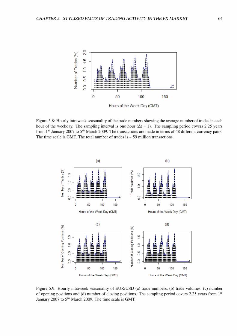
CHAPTER 5. STYLIZED FACTS OF TRADING ACTIVITY IN THE FX MARKET 64
Figure 5.8: Hourly intraweek seasonality of the trade numbers showing the average number of trades in eachhour of the weekday. The sampling interval is one hour (∆t = 1). The sampling period covers 2.25 yearsfrom 1st January 2007 to 5th March 2009. The transactions are made in terms of 48 different currency pairs.The time scale is GMT. The total number of trades is ~ 59 million transactions.
Figure 5.9: Hourly intraweek seasonality of EUR/USD (a) trade numbers, (b) trade volumes, (c) numberof opening positions and (d) number of closing positions. The sampling period covers 2.25 years from 1st
January 2007 to 5th March 2009. The time scale is GMT.

CHAPTER 5. STYLIZED FACTS OF TRADING ACTIVITY IN THE FX MARKET 65
Similarly to the intraday statistics, the intraweek statistics do not differ (a) for traders through different
currency pairs and with regard to the same currency pair (shown in Figures 5.8 and 5.9), and (b) over long
and short time horizons.
5.4 Correlation Behaviour
A convenient way to discover statistical properties of market trading activity is to conduct a correlation
study. The linear correlation coefficient is a measurement of the level of the dependence between variables.
It measures the relationship between two series of variables x and y, and is defined as follows:
corr(xi,yi) =∑
ni=1(xi− x)(yi− y)√
∑ni=1(xi− x)2 ∑
ni=1(yi− y)2
(5.20)
with the sample means:
x =n
∑i=1
xi
n(5.21)
y =n
∑i=1
yi
n(5.22)
For the stock market, it has been confirmed by a number of studies in the literature that intraday price
volatilities are correlated with the market activities in terms of the transaction data [106]. In contrast, for
the FX market there are relatively few studies on the intraday behaviour of market transactions due to the
difficulty of obtaining high-frequency data of market transactions. However, Dacorogna et al. in [63] found
across different currency pairs that the intraday volatilities are correlated with the activities measured in
terms of the tick numbers. Ito et al. in [117] found that the price changes and the trade volumes have a
positive correlation for the USD/YEN and the EUR/USD currency pairs they considered. In this section, we
present an analysis of the correlation function of EUR/USD trading activity and mid-price volatility. This is
done using hourly correlation calculation intervals over January, 1 2007 to January, 31 2009.
Figure 5.10 shows the correlation of EUR/USD hourly (a) trade numbers and volumes, (b) numbers of
buy and sell executed orders, and (c) numbers of opening and closing positions. We can see that the plots
in Figures 5.10 form an almost straight line sloping upwards to the right. These indicate a high positive
linear relationship between (a) trade numbers and volumes, (b) numbers of buy and sell executed orders,
and (c) numbers of opening and closing positions. The strength of the positive correlations is reflected in
their correlation coefficients, with the results reported in Table 5.4.
In Table 5.5, we can see some of the statistical properties of the hourly aggregated (a) trade numbers,
(b) trade volumes, (c) number of buy executed orders, (d) number of sell executed orders, (e) number of
opening positions and (f) number of closing positions. The basic descriptive statistic properties reported in
Table 5.5 are the mean, median, minimum, maximum and the standard deviation. From Table 5.5 we can
see that there are extremely close similarities between the statistical properties for the number of buy and
sell executed orders as well as for the number of opening and closing positions.
The volatility volL,t is a measure of the variation of market price pt at time t over a period of length L.
Given a price time series {pt , t ≥ 0} and given a period of length L, the volatility is defined as:
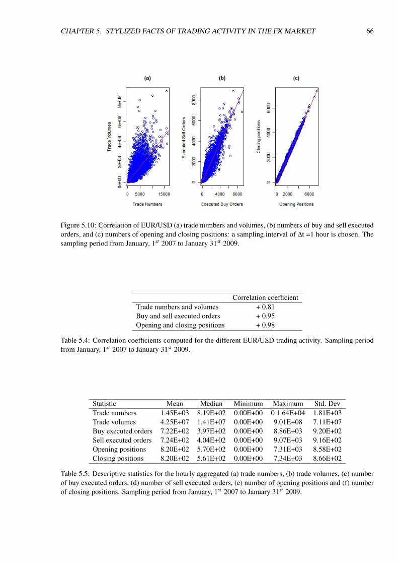
CHAPTER 5. STYLIZED FACTS OF TRADING ACTIVITY IN THE FX MARKET 66
Figure 5.10: Correlation of EUR/USD (a) trade numbers and volumes, (b) numbers of buy and sell executedorders, and (c) numbers of opening and closing positions: a sampling interval of ∆t =1 hour is chosen. Thesampling period from January, 1st 2007 to January 31st 2009.
Correlation coefficientTrade numbers and volumes + 0.81Buy and sell executed orders + 0.95Opening and closing positions + 0.98
Table 5.4: Correlation coefficients computed for the different EUR/USD trading activity. Sampling periodfrom January, 1st 2007 to January 31st 2009.
Statistic Mean Median Minimum Maximum Std. DevTrade numbers 1.45E+03 8.19E+02 0.00E+00 0 1.64E+04 1.81E+03Trade volumes 4.25E+07 1.41E+07 0.00E+00 9.01E+08 7.11E+07Buy executed orders 7.22E+02 3.97E+02 0.00E+00 8.86E+03 9.20E+02Sell executed orders 7.24E+02 4.04E+02 0.00E+00 9.07E+03 9.16E+02Opening positions 8.20E+02 5.70E+02 0.00E+00 7.31E+03 8.58E+02Closing positions 8.20E+02 5.61E+02 0.00E+00 7.34E+03 8.66E+02
Table 5.5: Descriptive statistics for the hourly aggregated (a) trade numbers, (b) trade volumes, (c) numberof buy executed orders, (d) number of sell executed orders, (e) number of opening positions and (f) numberof closing positions. Sampling period from January, 1st 2007 to January 31st 2009.

CHAPTER 5. STYLIZED FACTS OF TRADING ACTIVITY IN THE FX MARKET 67
volL,t =σ (pt , · · · , pt−L+1)
1L ∑
Li=1 pt−i
(5.23)
where σ is the standard deviation.
In this study, we found that the EUR/USD mid-price volatility of the last 24 hours is correlated with
the activities measured in terms of the trade numbers and volumes. The correlation coefficients computed
for the EUR/USD mid-price volatility of the last 24 hours and the trade numbers is +0.43 while for the
volumes it is + 0.28. We can hypothesise that an increase in the trade numbers would lead to a rise in the
price volatility, and vice versa. It is important to point out that this positive correlation does not mean that
changes in the price volatility cause changes in the trade numbers, and vice versa. To determine what causes
changes in terms of the direction of the trade numbers, an assessment of the overall market conditions must
be carried out.
5.5 Conclusion
In this chapter, we presented the study and analysis of the high frequency FX dataset provided by OANDA
Corporation with the aim being to establish the stylized facts of the trading activity in the FX market.
We undertook an analysis of the FX market traders’ collective behaviour which focused on: scaling laws,
seasonality statistics and correlation behaviour. Our contribution is two-fold. Firstly, using a HFD we
have been able to confirm a number of stylized facts apply on FX market transactions data that have been
described in the literature. Secondly, our work goes beyond those and we have discovered four new scaling
laws and six quantative relations among them apply on transactions data. These contributions are as follows:
• We have studied seasonality in the HF transactions dataset and have confirmed the existence of daily
and weekly periodic patterns in the FX market trading activity. This adds to the studies of [63, 117]
in the literature where they confirmed the existence of the double U-shape pattern of intraday trading
activities in FX markets [63, 117]. The intraday seasonality of trading activity can be explained by
considering the behaviour of worldwide FX market centres whose business trading hours partially
overlap. The intraweek seasonality can be explained by considering the daily patterns and the week-
end effect. The intraday and intraweek seasonality show that a high level of trading activity takes
place when two or more FX market centre business hours overlap. Trading activity peaks during the
opening business hours, declines during the lunch break, peaks again in the afternoon, then declines
gradually during the closing business hours of an FX market centre.
• We have investigated the correlation behaviour of high-frequency transactions data. This adds to
other studies reported in the literature [63, 117]. Our study is different in that we have explored the
correlation behaviour in different types of transaction in HF FX market data. It has been found that a
highly positive correlation exists between (a) trade numbers and volumes, (b) numbers of buy and sell
executed order, and (c) numbers of opening and closing positions. In addition, the price volatility of
the last 24 hours is correlated with the activities measured in terms of the trade numbers and volumes.
• The second main contribution of our study is the discovery of four new scaling laws and six quan-
titative relationships among them apply on transactions data (section 5.2.2). The statistical analysis
of the scaling laws is based on the directional-change event approach which is event driven and the

CHAPTER 5. STYLIZED FACTS OF TRADING ACTIVITY IN THE FX MARKET 68
scaling laws apply to transaction data. Given a fixed threshold (∆x), the observed four independent
new scaling laws state that the average (a) trade numbers, (b) trade volumes, numbers of (c) opening
and (d) closing positions observed during a price move of size ∆x is scale-invariant to the size of this
threshold. As far as we know this is the first such study that has studied and observed these relations.
This adds to Glattfelder et al.’s work [98] where they uncovered 12 independent new scaling laws in
foreign exchange price data.
Using the identified stylized facts presented in this chapter, in the next chapter we present the construction
of an agent-based FX market which we subsequently validate by testing its ability to reproduce and to what
extent the stylized facts of the trading activity of the real HF FX market.

Chapter 6
The Agent-Based FX Market
6.1 Introduction
The aim of our research is to identify the essential elements under which the stylized facts of the FX market
trading activity are exhibited in an ABM. In order to achieve our research aim, we use an agent-based
modelling approach to model the trading activity at the level of the FX market-maker high-frequency market.
The initial part of the study, chapter 5, is to observe the behaviour of the FX market traders in order to
establish the stylized facts of their collective trading activity in the market. This is performed using a high-
frequency dataset of anonymised individual traders’ historical transactions on an account level. The second
step, the subject of this chapter, is to build a simple and flexible agent-based FX market (ABFXM) which
is populated by a number of heterogeneous interacting agents. Using the identified stylized facts of the
FX market trading activity, we evaluate the trading activity produced from the ABFXM in resembling the
activity in the real market. By relating the stylized facts of actual FX market traders’ behaviour to the agent-
based models of traders, we may find a pathway to identify the essential elements necessary for modelling
the trading activity in the FX market.
The organization of this chapter is as follows. Section 6.2 presents the general setting of the ABFXM.
Section 6.3 describes how the market-maker works, whereas section 6.4 presents the available traded assets
in the market. The design of the trading agents is given in section 6.5. Next we present the trading cycle
in section 6.6, while section 6.7 provides a description of the market clearance. The design of the ABFXM
platform is giving in section 6.8. Section 6.9 provides the experimental and validation design to validate the
accuracy of the ABFXM in reproducing the stylized facts of the trading activity in the high-frequency FX
market. The results of the experiments that have been performed are presented in section 6.9. The chapter
ends with the conclusions in section 6.10.
6.2 General Setting of the ABFXM
The agent-based FX market (ABFXM) simulates the trading activity at the level of an FX market-maker
high-frequency market. The constituent elements in the market are N heterogeneous agents as described in
the following subsections who interact through buying and selling currencies in the market via the market-
maker. Figure 6.1 shows the main components of the simulation and their interaction.
We focus our attention on the impact that changes on the agents’ structural elements (and consequently
behaviour) have on the intensity and flow of market trading activity and for this purpose we use a dataset
69

CHAPTER 6. THE AGENT-BASED FX MARKET 70
Figure 6.1: The main components of the ABFXM and their interaction.
of high-frequency historical prices for EUR/USD currency pair and feed these prices into the simulation
via the market-maker. The prices are fed over a defined one month period and hence the agents react on
such information. We use this dataset as the purpose of this work is to develop an ABFXM that is able to
approximate the stylized facts of trading activity that are exhibited in the real FX market data and explore
their origins. These stylized facts relate to transactions data (a transaction represents an executable order
in the market) and hence the price data are used to anchor the simulation results so that we can establish
whether the transactions data generated by the ABFXM have the same characteristics and properties as the
real market data. The historical dataset of prices acts as a constant so that multiple simulation runs can
be performed in which aspects of the trading behaviour of the agents can be modified and systematically
studied without having to worry about price setting in the market. This enables us to study the ensuing
behaviour and data generated from the market against those of the real market and also compare different
settings against one another.
We consider N agents divided equally into NContrary contrary agents and NTrend trend following agents
(N = NContrary + NTrend ), to be further explained in section 6.5.5. An agent takes a decision at time t of
the simulation, based on its budget constraints and preferences, to be explained in depth in the following
sections. Prior to the start of the simulation, based on a continuous uniform distribution, each individual
agent will be assigned the following elements:
• Home currency: the agent account’s primary currency.
• Leverage: this is the ratio of the margin to the maximum trade size. For example, with a deposit of
$1,000 and a leverage of 20:1, a trader could open a position in which the position value is $20,000.
Trading on margin is explained in section 6.5.2.
• Business trading hours correspond to a FX trading session as explained in section 6.5.9.2.
• Profit objective and risk appetite thresholds are as explained in section 6.5.4.
In addition to the above elements, each individual agent will be endowed with a different amount of cash

CHAPTER 6. THE AGENT-BASED FX MARKET 71
(wealth) expressed in the agent’s home currency. The wealth distribution is based on a power law distribu-
tion, as explained in section 6.5.1.
The trading activities of each individual agent as well as its portfolio, will be recorded on external text
files for analytical purposes. Furthermore, all the necessary statistics of each trading round will be stored on
external text files to allow further analysis.
6.3 The Market-Maker
An FX market-maker is a corporation which supplies liquidity for a number of currency pairs, and conse-
quently quotes both a buy and a sell price for a currency pair on its platform. The market-maker buys from
and sells to its investors and other market-makers and hence makes a profit on the bid-offer spread. The FX
market-maker quotes the bid and ask price for a currency pair on its platform by observing the demand and
supply in the market, historical information, their inventory holdings, prices from other market-makers, and
information about current political and economic events, as well as other factors.
The ABFXM developed consists of an FX market-maker which quotes prices and trading agents who
participate in the market by means of buying and selling currencies. The market-maker uses a historical
high-frequency prices dataset to issue price quotes as explained in section 6.2. As part of future work we
aim to explore the generation of artificial prices in the ABFXM using one or more FX market-makers. This
will allow studying price formation through the FX market-maker component. But for the purposes of this
work the prices had to be fed through the historical high-frequency prices dataset.
6.4 Assets
At any time t in the market, an agent j is capable of holding two different types of assets:
• A risk free asset in the form of cash.
• A risky asset in the form of a currency pair (EUR/USD).
The decision behind having just two different types of assets was based primarily on the complexity of the
analysis of markets in which more than two assets are available for trading [137]. However, according to
LeBaron [137] there are a few ABMs, in which more than two assets can be traded such as [49, 229]. The
leading influential work in the area of ABMs, Santa Fe Artificial Stock Market (SF ASM), is composed of
two tradable assets, a risk-free bond and a risky stock asset [140]. Examples of ABMs composed of two
tradable assets are the ones developed by [5, 171].
A currency pair in the market is represented as a base and a quote (base/quote) in which these two
currencies are traded. For example, the base of EUR/USD is EUR while the quote is USD. We denote bt
at time t as the bid price at which a trader can sell the base currency and buy an equivalent amount of the
quoted currency to buy the base currency. This means a trader opening a short position. Similarly, the ask
price at at time t is the offer rate at which a trader can buy the base currency and sell an equivalent amount
of the quoted currency to pay for the base currency, opening a long position.
CHAPTER 6. THE AGENT-BASED FX MARKET 72
6.5 Agent Design
In designing trading agents, there are two equally important but competing principles/imperatives that we
need to keep in mind. On the one hand, simplicity is key as a complex agent and in more general market
design may impede the study, understanding and interpretation of the origins of the stylized facts [110] and
in general the dynamics of the market. On the other hand, heterogeneity is inherent in real markets and they
are populated by agents who have different preferences, demands, aspirations, trading strategies and trading
hours. Some of the previous works in ABMs do not consider heterogeneity in the agent’s preferences and
the agents are allocated the same profit objectives, time horizons, forecasting and decision making horizons
[137]. In our work, we have attempted to satisfy both of these principles through a well-defined parameter
space and clear strategy. In our agent-based model of traders, heterogeneity exists in (a) wealth variations
among the agents; (b) different behavioural groups of ZI-DCT0 agents; (c) agents who have different profit
objectives; (d) agents who have different risk appetites that form long and short term investors; and finally
(e) agents who use different trading time windows. All of these aspects build heterogeneity into the trading
model, leading to the characterization of different trading activities. The following sections describe the
various elements of the agents’ design and their by default setting.
6.5.1 Initial Wealth Distribution
The wealth represents the amount of cash that an agent holds and it is expressed in the home currency of the
agent’s account. Many ABMs imply that all agents are endowed with the same amount of cash prior to the
launch of the simulation, as has been done by [64, 124, 140, 150, 172].
In our ABFXM, we use a power law distribution to endow each agent with a different amount of cash1.
The motivation for choosing a power-law distribution rather than other distribution methods is that our
target in building models of the market traders is to reproduce stylized facts of the financial markets. Over a
century ago, Pareto found through empirical observation, that the income distribution in numerous countries
follows a power-law distribution [186]. In the follow-up of Pareto’s study, a number of empirical studies
support this hypothesis by providing evidence from empirical data [22, 185, 209]. We quantify the income
distribution in financial markets by the income distribution of a country’s population. Hence, we use a power
law distribution to endow each agent with a different amount of cash which is a more accurate reflection of
what happens in reality.
The power-law distribution is employed in the simulation by converting a random number that is uni-
formly distributed into a number that is distributed along the power-law distribution. The power-law and the
random variable are related via: ˆ l1
l0k.l−α =
zˆ
0
1dz (6.1)
where l0 and l1 are the lower and upper bounds respectively from which the power law distribution
holds. k is a constant value defined by:
k =−α +1
l(−α+1)1 − l(−α+1)
0
(6.2)
1In the subsequent chapter (chapter 7), we examine the impact of different distribution methods for the agents’ initial wealth inthe exhibition of the market trading activity’s stylized facts. Moreover, we show that the selection of a power law distribution forthe agents’ initial wealth is capable of reproducing, to a certain extent, the stylized facts of FX market trading activity.

CHAPTER 6. THE AGENT-BASED FX MARKET 73
α is the scaling exponent for a power-law distribution and z is a random number drawn from a uniformly
distributed number. Combining these two equations, the power law has the following form:
lz =(
z(−α +1)k
+ l(−α+1)0
)(−α+1)
(6.3)
Estimating the value of the scaling exponent for a power-law distribution is very important due to its
role in characterising the distribution. Caution in estimating the scaling exponent is essential. The larger the
scaling exponent, the steeper the curve, consequently implying more small scales than large ones.
6.5.2 Margin Trading
Trading on margins enables a trader to place an order where the order size is larger than his cash holding.
Trading on margins involves borrowing a fraction of the cash required from the market-maker executing
the transaction. Nevertheless, trading on margins is dependent on the leverage ratio used by the trader. A
leverage ratio of v:1 is a minimum margin requirement of m% ( 1v ). This means that if a trader decides to
open a new position, it must have at least m% of the position’s size available as a margin. Traders trading on
the margin may possibly realize a high profit, but this in turn involves a high risk. Accordingly, trading on
the margin makes use of a course of action so-called a margin call. The margin-call procedure is explained
in section 6.7.
6.5.3 Portfolio
Every agent j has a portfolio which records the results of the agent’s financial transactions. A portfolio is
associated with the agent’s account home currency. In an agent’s portfolio, the following information is
recorded:
Balance: The amount of cash in the agent’s account. It is denoted by c j,t at time t. The balance is
expressed based on the agent’s home currency. An agent’s balance changes when the agent realizes a profit
or loss on a closed position. The balance does not change with the current exchange rate on the agent’s open
positions.
Unrealized profits and losses: The profits or losses that would be produced if an agent j’s open position
were closed at the current currency pair price, denoted by go, j,t for position o at time t. For a long position,
go, j,t is computed by:
go, j,t = (bt −op)× (ro×os) (6.4)
For a short position, go, j,t is computed by:
go, j,t = (op−at)× (ro×os) (6.5)
where
bt is the current bid price of the position currency pair;
at is the current ask price of the position currency pair;
op is the price at which the position was opened;
os is the position size;

CHAPTER 6. THE AGENT-BASED FX MARKET 74
(ro× os) is the size of the position (in units) converted from the quote currency of the currency pair in
question to the agent’s home currency using the current ask price if the position is short and the current bid
price if the position is long.
Once an agent closes a position and has realized a profit, this will be added to the agent’s balance,
whereas if the position has realized losses, the opposite will be the case.
Net Asset Value (NAV): The NAV at time t represents the current value of an account, denoted by
NAVj,t . In other words, NAVj,t is the amount of cash in agent j’s account, plus all unrealized profits and
minus all unrealized losses associated with all the account’s open positions. If an agent has no open position
at time t, the NAV is basically equal to the amount of cash in the account balance. NAVj,t is computed as:
NAVj,t = c j,t +n
∑o=1
go, j,t (6.6)
where
c j,t denotes the amount of cash in agent j’s account;
n is the current number of positions held by agent j at time t;
go, j,t is the unrealized gains or losses associated with position o, computed from Equation 6.4 (long
position) or Equation 6.5 (short position).
Margin used: The margin used is denoted by m j,t at time t. This amount is equal to the position value
multiplied by the agent’s margin ratio, summed up over all the agent’s open positions. The margin ratio is
the inverse of the used leverage v j. For example, a 20:1 leverage equals a 0.05 margin ratio. If an agent
has no open position at time t, the margin used is in essence equal to zero. The margin used at time t is
computed as:
m j,t =n
∑o=1
ro×os
v j(6.7)
where
n is the number of positions held by the agent at time t;
os is the position size;
v j is agent j’s used leverage;
(ro× os) is the size of the position (in units) converted from the base currency of the currency pair in
question to the agent’s account currency using the current ask price if the position is long and the current
bid price if the position is short.
Margin available: The amount of the agent’s balance and unrealized profit and losses available as a
margin for a new trade. In detail, the margin available is equal to the agent’s net asset value NAVj,t minus
the margin used m j,t . If the margin available is 0, then the agent cannot open new positions or increase
existing positions. The margin available is denoted by MA j,t and is computed at time t by:
MA j,t = NAVj,t −m j,t (6.8)
6.5.4 Profit Objective and Risk Appetite
The traders’ profit objectives and risk appetite affects and characterizes the volume and flow of market
trading activity. Accordingly, using the high-frequency individual traders’ transactions dataset, we map the
traders’ profit objectives and risk appetites into the agent-based models of traders.

CHAPTER 6. THE AGENT-BASED FX MARKET 75
The mapping was accomplished through tracking each trader’s transactions in each of their traded cur-
rency pairs. Specifically, this is done in terms of tracing the number of currency units bought and sold
sequentially by the transactions’ execution time. Consequently, we trace a trader’s different types of orders
with regard to a given currency pair from the opening to the closing of a position. This allows us to define
the trader’s profit and loss thresholds by which the trader decides to open and close their positions. The
threshold represents the size of price movements as a result of which a trader decides to place a new order.
From this analysis, we conclude with the following two observations:
• In terms of the traders’ profit objectives, the majority of traders place a new order based on small
changes in the price. For that reason, based on a uniform distribution, the profit objective thresholds
will be generated for each individual agent by drawing random numbers from a uniform narrow in-
terval [0.01%, 2%]. The limits of such intervals are important for reproducing the real FX market
trading activity.
• In contrast, the length of the traders’ holdings on losing positions tends to be extensive. This indicates
that many of the trading strategies of real traders involve a high degree of risk. This fact was mapped
into the agent-based models of traders in which we defined the agents’ risk appetites to be four times
their profit objectives. The choice of this setting was based on a number of controlled experiments
further explained in chapter 7.
Since the profit objective and risk appetite thresholds differ amongst agents, we consider each agent to be a
unique trader which adds to the heterogeneity in our model.
6.5.5 Trading Strategy
The agents’ adopt the zero-intelligence directional-change event trading strategy (ZI-DCT0), described in
chapter 3. The central idea behind ZI-DCT0 is that an agent will observe the changes in the price time
series and commit to a fixed threshold based on intrinsic time rather than physical time. Physical time
adopts a point-based system and is homogenous with time scales equally spaced based on the chosen time
unit (second, minutes, etc.). In contrast, intrinsic time is irregularly-spaced in time as time triggers just at
periodic events [98]. The intrinsic time basic unit is an event which is defined as the total price change
exceeding a given fixed threshold defined by the agent.
For studying an asset’s price time series, given a fixed threshold of size ∆x, the absolute price change
between two local minimum and maximum prices is decomposed into a directional-change (DC) event of
size ∆x and its associated overshoot (OS) event [98]. The OS event represents the price movement beyond
the fixed threshold ∆x. A DC event takes one of the two forms - an upturn DC event or a downturn DC
event [219]. An upward run is a period between an upturn DC event and the next downturn DC event,
while a downward run is a period between a downturn DC event and the next upturn DC event. An upturn
(downturn) DC event ends a downward (upward) run, and starts an upward (downward) run.
Before the study of an asset’s price time series, two variables are defined: the last high and low prices
which are set to the asset’s price at the start of the price sequence [219]. During an upward run, the last high
price is continuously updated to the maximum of (a) the current price and (b) the last high price. During the
period of a downward run, the last low price is continuously updated to (a) the minimum of the current price
and (b) the last low price. An upturn DC event occurs once the absolute price change between the current
price and the last low price is higher than the threshold of size ∆x, while a downturn DC event occurs once

CHAPTER 6. THE AGENT-BASED FX MARKET 76
Algorithm 6.1 The core trading mechanism for the two groups of ZI-DCT0 agentsRequire: initialise variables (event is upturn event, x =pt ,4xDC (Fixed ) ≥ 0)if event is upturn event then
if pt ≤ x× (1−4xDC)event← downturn eventx← pt
Buy→ZI-DCT0 contrarian agent, Sell→ZI-DCT0 trend follower agentelse
x← max ( x, pt)end if
else //Event is downturn eventif pt ≥ x× (1+4xDC) then
event← Upturn eventx← pt
Sell→ZI-DCT0 contrarian agent, Buy→ZI-DCT0 trend follower agentelse
x← min ( x, pt)end if
endif
the absolute price change between the current price and the last high price is lower than the threshold of size
∆x.
Before the launch of the simulation, based on a continuous uniform distribution, each ZI-DCT0 agent
assigns a fixed threshold from a uniform interval [0.01%, 2%]. Two different equal groups of agents are
identified based on ZI-DCT0: contrary and trend-following agents. A contrary agent opens a new position
in the prediction that the price will move in the opposite direction. For instance, an agent may open a
new long position when the price falls by 0.04% and afterwards closes the position as soon as the price
rises by 0.06%. By way of illustration, a contrary agent opens a new short (long) position if the current
bid (ask) price rises (declines) by a percentage which is equal to, or above, the threshold defined based on
the agent’s expectation of the market. Trend-following agents take advantage of the price trend movement
direction, assuming that the current trend will continue in the same direction. A trend follower agent opens
a new long position whilst the price is rising, whereas a short position is opened when the price is falling.
Hence, a trend follower opens a new short (long) position if the current bid (ask) price declines (rises) by a
percentage which is equal to, or above, the threshold used by the agent. Algorithm 6.1 illustrates the core
trading mechanism for these two groups of ZI-DCT0 agents.
The buying and selling orders placed by these two groups of agents are market orders. These market
orders are orders for immediate execution at the current price of a currency in the market. There is assurance
with regard to the execution of a market order, but ambiguity concerning the execution price. For a market
order, an agent specifies the order size and type, with the order type being either a buy or a sell order.
A position is opened once an agent has bought or short-sold any quantity of currency units. A position
can be of type long (bought) or short (sold). The position volume stands for the number of bought or sold
currency units executed in the market. The position price is the unit price at which the position was opened.
The position closure takes place as a result of either a margin call or an agent’s decisions through market or
limit orders, to be explained in sections 6.5.6, 6.6 and 6.7.
A similar trading strategy to the ZI-DCT0 was introduced by [5] in which the agents enter the market and
operate in it only if the price fluctuations are above a certain threshold. The threshold remains constant and

CHAPTER 6. THE AGENT-BASED FX MARKET 77
is defined for each agent before the launch of the market. Furthermore, the authors suggest that introducing
a threshold in terms of the agents’ activities, which modulates the number of active agents in the market, is
one of the factors responsible for the exhibition of stylized facts in an ABM. The main differences between
the adopted ZI-DCT0 trading strategy in our ABFXM and the one introduced by [5], is that the former
considers the direction and the overshoot of the price movement in the agent trading activities, whereas the
latter does not.
6.5.6 Limit Orders
To acquire a comprehensive trading strategy for the agents, we incorporate two types of limit orders; profit-
taking and stop-loss limit orders. For limit orders, a trader must declare the price at which it desires to close
its current opened position. There is no guarantee that the declared price will be reached and as a result the
execution of a limit order is not guaranteed. If a limit order is executed, there is a guarantee with regard to
the execution price.
The profit taking limit order is an order to close a position once a certain profit threshold is reached to
lock in a certain profit realization. The profit taking limit order is determined with reference to the agent’s
profit objective. For instance, for closing a long position the bidding price for the profit taking limit order
must be higher than the purchasing price, while for closing a short position, the asking price for the profit
taking limit order must be less than the selling price.
The stop-loss limit order is an order to close a position once a loss threshold has been reached. Such a
threshold is defined by the agent, subject to its risk appetite. For closing a long position, a stop-loss limit
order becomes a market order after the bid price is at, or below, a specified loss threshold price (stop price)
determined by the agent. On the other hand, for closing a short position, a stop-loss limit order becomes a
market order after the ask price is at or above a specified stop price as defined by the agent. A stop-loss limit
order seeks to limit the loss potential for a position.
The generation of profit-taking and stop-loss limit orders in the market has significant impact on re-
producing the stylized facts of FX market trading activity as shown in subsequent experiments in chapter
7.
6.5.7 Random Trade
Market traders place orders based on factors other than price movements (e.g. economic and political
events). In our ABFXM, this is modelled by incorporating random trading into the agents’ trading strategies.
A random trade represents a trade placed beyond the notion of changes in price time series. When an agent’s
trading conditions are not met, it will place a random trade based on a probability equal to 10−6. Such a
probability is defined before the simulation starts, and remains constant during the simulation.
6.5.8 Order Size
The order size is an important element of our simulation since it is associated with the cautiousness of the
agents. In the ABM literature, there are two main approaches to determining a single order size placed by an
agent in an ABM. The direct approach entails an agent’s order size being proportional to the agent’s wealth
such as in [193]. This simple approach creates an extremely high trading risk, given that an agent invests
its total cash in a single order. The second approach assumes that an agent’s order size is a fraction of its

CHAPTER 6. THE AGENT-BASED FX MARKET 78
cash such as in [172, 212]. The fraction value is determined by a constant trading proportion parameter.
Experiments using the methods in [172, 193, 212] have been carried out in chapter 7.
In our ABFXM, we follow a different approach and the determination of the number of currency units
depends on the agent’s available margin. In detail, an order’s size is determined randomly within a specified
range [UA × 10%, UA], based on the number of currency units the agent has available (UA) to trade.
Unit Available (UA) is the maximum number of currency units an agent is allowed to trade, subject to the
agent’s available margin. For an order, the minimum number of currency units is 10% of the UA, while the
maximum is equal to UA. Equation 6.9 clarifies how to calculate agent j’s currency units available (UA) to
trade.
UA j,t =MA j,t
v j× r(6.9)
where
MA j,t is the margin available for agent j, calculated from equation 6.8;
v j is the leverage used by agent j;
r is the exchange rate of the base currency of the currency pair in relation to the agent’s account currency
using the current ask price if the position is long and the current bid price if the position is short.
This new proposed approach for characterizing an agent order size in the market is sufficient since it
generates a source of heterogeneity in the agent investment strategy which affects the fluctuations in price
in the market. A stable market is unappealing for traders, while the existence of various changes in the price
movements attracts traders to participate [7].
6.5.9 Asynchronous Trading Time Window
Some ABMs imply continuous-time which means that at period t of the market, all agents send their orders
and then agents update their beliefs to go to the next period t+1. This synchronous representation of time is
not fitting for high-frequency data. The studies by Boer et al. [40] and Daniel [64] show that the dynamics
of the ABM differ extensively, according to whether the state of the ABM is updated in continuous-time
or in discrete-time. Their findings conclude that the asynchronous nature of trading in financial markets
essentially has to be considered in agent-based models of financial markets.
The Grand Canonical Minority Game [120] and CHASM [172] adopt discrete-time trading in which the
model allows agents to place an order or to hold. Accordingly, the number of agents participating in the
total demand and supply is not constant at every time period of the market. Unfortunately, such a model
does not present a realistic level of synchronisation, given that at every time period of the market, each agent
has to carry out some trading computation. An alternative approach is introduced in the Genoa Artificial
Stock Market [188] in which the determination of the agents who will be active in the next period is drawn
randomly. Such randomisation alone is not sufficient as it would be ambiguous for the arrival time of the
order.
In modelling an asynchronous trading time window for the agents, we addressed this critical modelling
issue by considering three important factors: the agents’ activation time in the market, the notion of market
business hours, and holidays.

CHAPTER 6. THE AGENT-BASED FX MARKET 79
Market Opening time closing timeTokyo 00:00:00 08:00:00
London 08:00:00 16:00:00New York 13:00:00 21:00:00
Sydney 22:00:00 06:00:00
Table 6.1: FX market opening and closing business time for different market sessions. The time zone isGMT. The markets are listed in the order of their opening times in GMT. (as reported in Table 5.3)
6.5.9.1 Initial Activation Condition
As it is the case in real markets, not all agents are active at the launch of the simulation. We have set up the
initial activation condition to control when an agent will start to be active in the market for the first time. Our
condition is based on a probability equal to 10−2 which is defined before the simulation starts, and remains
constant during the simulation.
6.5.9.2 Business Hours and Holidays
Contrary to the stock market, the FX market does not imply a fixed trading time window giving the traders
24 hours a day to operate. However, the differences in the worldwide FX market centres’ business hours
have a tangible effect on the dynamics of FX market trading activity, mainly during the overlapping business
hours when two or more market centres are open simultaneously. This is because the worldwide FX market
centres located in different time zones have different business trading hours and traders’ preferences. The
different business trading hours and traders’ preferences, without a doubt, characterize, and determine, the
intensity of trading activity in the market. Table 6.1 presents local business trading hours of different FX
market trading sessions that are identified based on [63].
In our simulation, each agent is associated with local market business trading hours corresponding to its
geographical location. This in essence means that although an agent can trade at any time during the day,
the probability of doing so outside its business hours is restricted based on a very small probability equal to
10−6(except for executing limit orders).
6.6 Trading Cycle
We make the following four assumptions in modelling the agents’ trading mechanism:
Assumption 1 We assume that a position cannot be adjusted.
Assumption 2 A position is only opened by a market order or a limit order.
Assumption 3 We restrict the quantity of positions held by an agent j at time t to be one opened position.
Assumption 4 The market does not imply fees for the transactions.
Basically the main reason for these simplification assumptions is that by making these assumptions
the complexity of the behaviour of the model is reduced to a level that can be studied within the scope of
this work. Simplicity is fundamental to clearly understand the agents’ trading behaviour. Thus, allocating
variable quantities results in a considerable complication of the analysis. The relaxation of these four as-
sumptions does not affect the generality of the simulation results presented in our study. However, we are
aware of the importance of the role of quantity as a choice variable, especially with risk aversion.
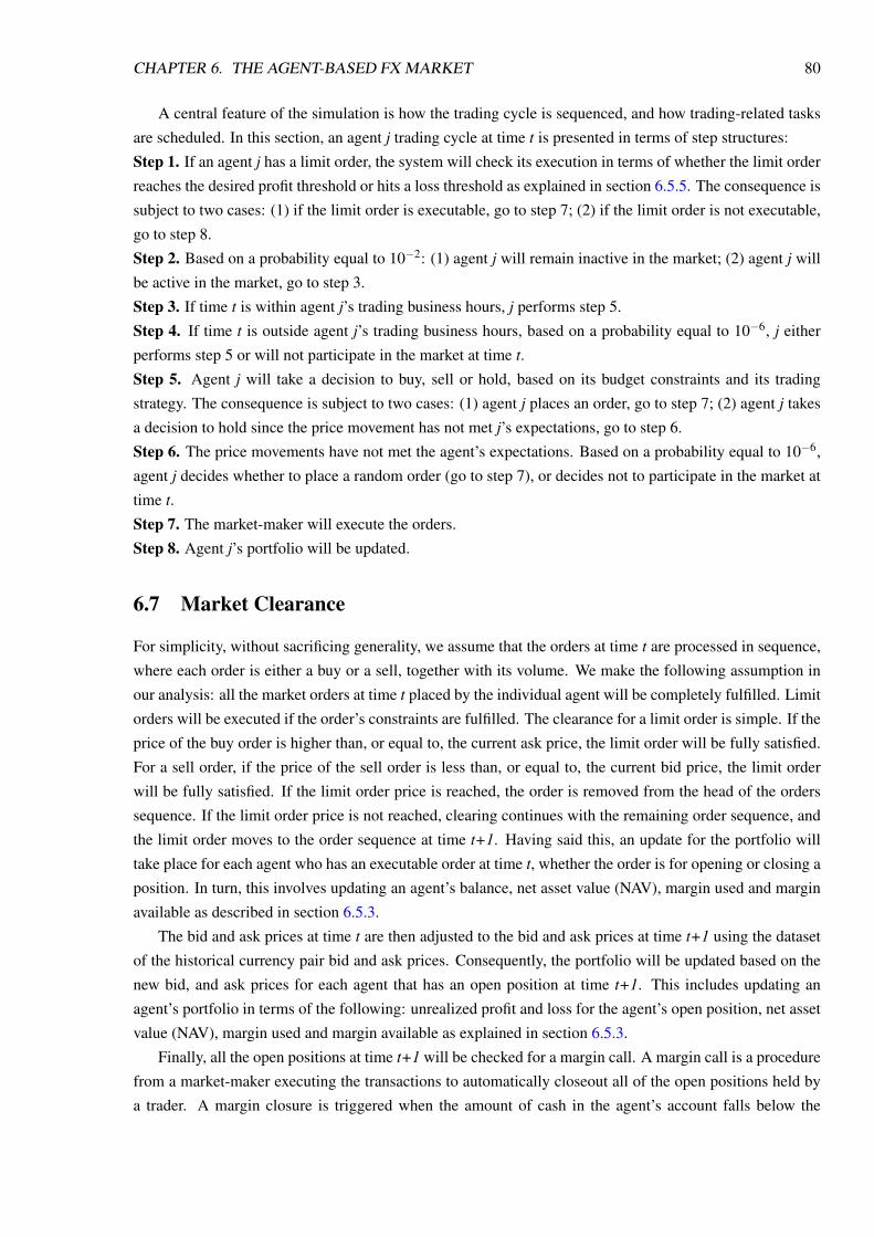
CHAPTER 6. THE AGENT-BASED FX MARKET 80
A central feature of the simulation is how the trading cycle is sequenced, and how trading-related tasks
are scheduled. In this section, an agent j trading cycle at time t is presented in terms of step structures:
Step 1. If an agent j has a limit order, the system will check its execution in terms of whether the limit order
reaches the desired profit threshold or hits a loss threshold as explained in section 6.5.5. The consequence is
subject to two cases: (1) if the limit order is executable, go to step 7; (2) if the limit order is not executable,
go to step 8.
Step 2. Based on a probability equal to 10−2: (1) agent j will remain inactive in the market; (2) agent j will
be active in the market, go to step 3.
Step 3. If time t is within agent j’s trading business hours, j performs step 5.
Step 4. If time t is outside agent j’s trading business hours, based on a probability equal to 10−6, j either
performs step 5 or will not participate in the market at time t.
Step 5. Agent j will take a decision to buy, sell or hold, based on its budget constraints and its trading
strategy. The consequence is subject to two cases: (1) agent j places an order, go to step 7; (2) agent j takes
a decision to hold since the price movement has not met j’s expectations, go to step 6.
Step 6. The price movements have not met the agent’s expectations. Based on a probability equal to 10−6,
agent j decides whether to place a random order (go to step 7), or decides not to participate in the market at
time t.
Step 7. The market-maker will execute the orders.
Step 8. Agent j’s portfolio will be updated.
6.7 Market Clearance
For simplicity, without sacrificing generality, we assume that the orders at time t are processed in sequence,
where each order is either a buy or a sell, together with its volume. We make the following assumption in
our analysis: all the market orders at time t placed by the individual agent will be completely fulfilled. Limit
orders will be executed if the order’s constraints are fulfilled. The clearance for a limit order is simple. If the
price of the buy order is higher than, or equal to, the current ask price, the limit order will be fully satisfied.
For a sell order, if the price of the sell order is less than, or equal to, the current bid price, the limit order
will be fully satisfied. If the limit order price is reached, the order is removed from the head of the orders
sequence. If the limit order price is not reached, clearing continues with the remaining order sequence, and
the limit order moves to the order sequence at time t+1. Having said this, an update for the portfolio will
take place for each agent who has an executable order at time t, whether the order is for opening or closing a
position. In turn, this involves updating an agent’s balance, net asset value (NAV), margin used and margin
available as described in section 6.5.3.
The bid and ask prices at time t are then adjusted to the bid and ask prices at time t+1 using the dataset
of the historical currency pair bid and ask prices. Consequently, the portfolio will be updated based on the
new bid, and ask prices for each agent that has an open position at time t+1. This includes updating an
agent’s portfolio in terms of the following: unrealized profit and loss for the agent’s open position, net asset
value (NAV), margin used and margin available as explained in section 6.5.3.
Finally, all the open positions at time t+1 will be checked for a margin call. A margin call is a procedure
from a market-maker executing the transactions to automatically closeout all of the open positions held by
a trader. A margin closure is triggered when the amount of cash in the agent’s account falls below the

CHAPTER 6. THE AGENT-BASED FX MARKET 81
minimum margin needed to cover the size of its currently open position. Furthermore, a position closure
triggered from a margin call, means selling (buying) the currency units an agent holds (short) at the current
bid (ask) price. The intention of the margin call procedure is to prevent a trader from losing more than the
amount of cash in its account. Equation 6.10 illustrates how to compute the margin call for an agent j’s open
position.
NAVj,t ≤m j,t
2(6.10)
where NAVj,t denotes the net asset value (NAV) and m j,t denotes the margin used for agent j at time t.
When the condition of an agent’s used margin is exceeded, consequently the agent’s open position
triggers a margin call to close up the position and the realized losses will be subtracted from the agent’s
balance. The agent’s portfolio will be updated. In particular, the agent’s net asset value and margin available
will be both equal to the amount of cash in the account balance. The amount of margin used by the agent
will be reset to zero. If an agent’s balance goes to zero, then the agent is removed from the market.
6.8 The Platform
The platform of the ABFXM developed in Java provides a computer environment in which the modeller can
build agent-based model of the FX market to explore the market traders’ behaviour by means of simulations.
The ABFXM platform is capable of providing the functionalities of scenario and sensitivity analysis. In
designing the ABFXM platform, we have considered four essential properties, which are as follows:
• The platform should be easy to modify in order to be able to change features specific to the market.
• The platform should be easily extensible to allow for new functionalities to be added.
• The implementation of a graphic user interface for the ABFXM is required. This facilitates the use
of the ABFXM, given the difficulties of tracking changes in the market parameters and features in a
systematic way. Moreover, the graphic user interface allows direct access to the different parameters
involved in the ABFXM which in turn facilitates the possibility of different experimentations on the
part of the user.
• The graphic user interface should allow the user to execute different scenarios to examine different
important features of the market. For example, the user can examine the effect of different order sizes
in the market.
The user can run the simulation for a predefined number of trading periods or for a given time, say, one
simulated month. The progression of the simulation can be monitored by means of panels that offer a visu-
alization of the price level, the total and average wealth of the agents, the volume of buy and sell executed
orders, etc. Figure 6.2 presents a screen shot of the platform’s main screen. The tools presented in Figure
6.2 are for monitoring the progression of the simulation in real-time, which is helpful for the immediate
debugging and modification of the parameters and features involved in the ABFXM. The simulation can
be reset to its initial configuration while changing just the random seed, to allow for evaluations between
different runs in order to assess the robustness of the ABFXM to the initial configuration. A systematic
exploration of the ABFXM’s parameters can be conducted. Figure 6.3, 6.4 and 6.5 capture the main pa-
rameters’ windows. These parameters are available to the user to modify and explore the ABFXM under
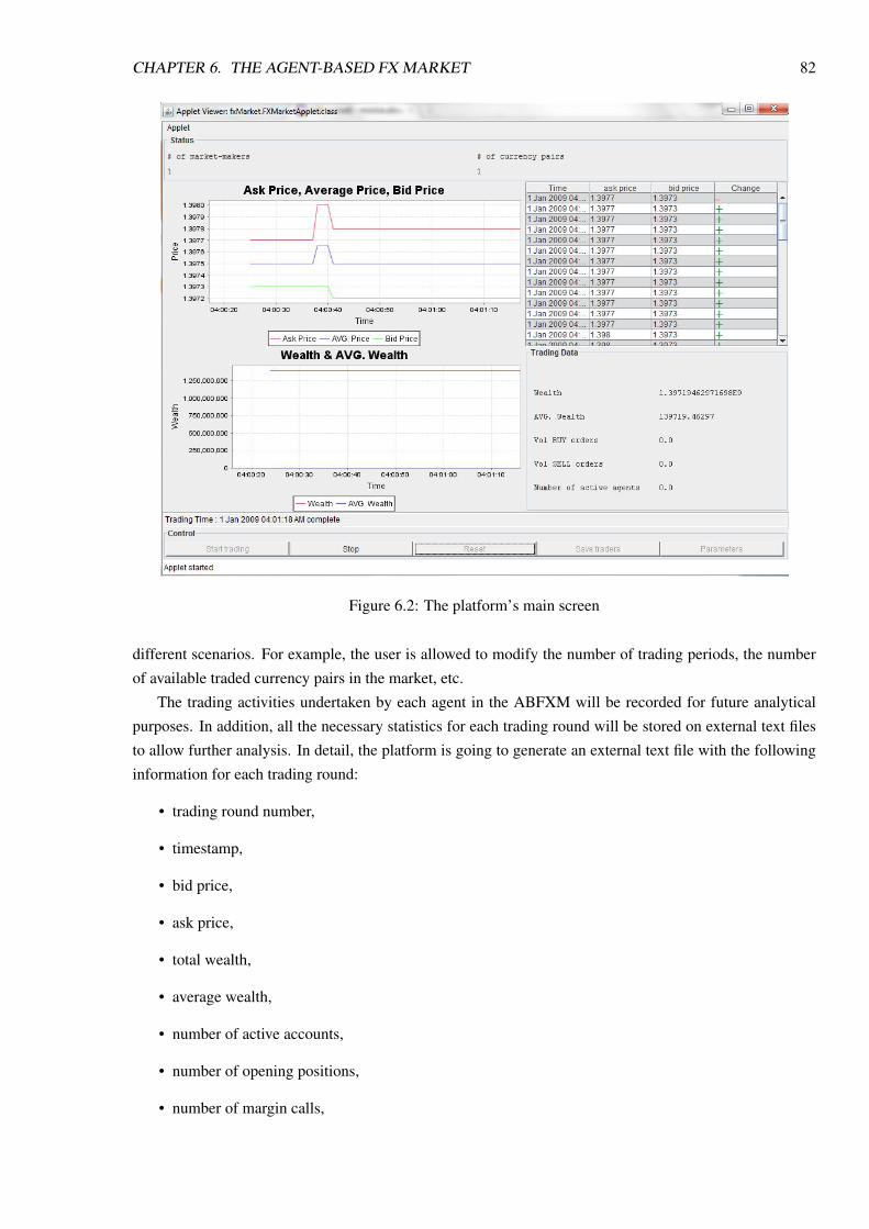
CHAPTER 6. THE AGENT-BASED FX MARKET 82
Figure 6.2: The platform’s main screen
different scenarios. For example, the user is allowed to modify the number of trading periods, the number
of available traded currency pairs in the market, etc.
The trading activities undertaken by each agent in the ABFXM will be recorded for future analytical
purposes. In addition, all the necessary statistics for each trading round will be stored on external text files
to allow further analysis. In detail, the platform is going to generate an external text file with the following
information for each trading round:
• trading round number,
• timestamp,
• bid price,
• ask price,
• total wealth,
• average wealth,
• number of active accounts,
• number of opening positions,
• number of margin calls,
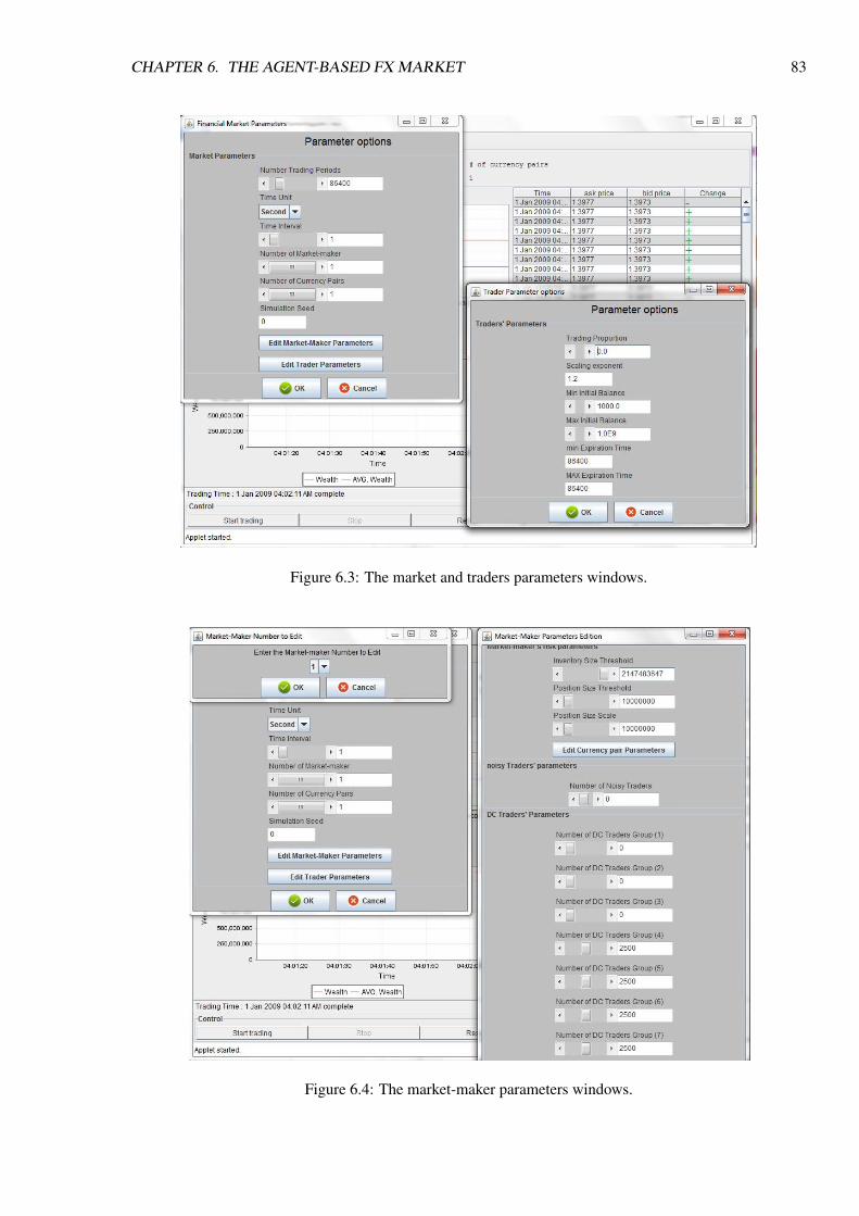
CHAPTER 6. THE AGENT-BASED FX MARKET 83
Figure 6.3: The market and traders parameters windows.
Figure 6.4: The market-maker parameters windows.

CHAPTER 6. THE AGENT-BASED FX MARKET 84
Figure 6.5: The currency-pair parameters window.
• number of opening long positions,
• number of opening short positions,
• number of closing long positions,
• number of closing short positions,
• volume of opening long positions,
• volume of opening short positions,
• volume of closing long positions,
• volume of closing short positions,
• number of buy executed orders,
• number of sell executed orders,
• volume of buy executed orders,
• volume of sell executed orders,
• number of closing long positions in profit,
• number of closing short positions in profit,
• number of closing long positions at a loss,
CHAPTER 6. THE AGENT-BASED FX MARKET 85
• number of closing short positions at a loss,
• volume of closing long positions in profit,
• volume of closing short positions in profit,
• volume of closing long positions at a loss and
• volume of closing short positions at a loss.
The designed platform is very flexible allowing the user to easily modify the different parameters and fea-
tures involved in the ABFXM in a systematic way. For instance, the user can easily change the method of the
agents’ initial wealth distribution and also the distribution of the agents’ profit objectives and their trading
time windows. The user could generate or forbid the generation of limit orders in the ABFXM. Moreover,
the user can model different levels of the agents’ risk appetites in the market. These modifications allow the
user to examine the implications of the different parameters and features involved in the ABFXM in order
to understand the market behaviour, and the different economic hypotheses.
With regard to the extensibility of the ABFXM, it is a straightforward task to include new functionalities.
For instance, the ABFXM can be extended to permit more than one traded asset (currency pair). Addition-
ally, the ABFXM can be easily extended to generate artificial prices resembling the FX market time series
with regard to prices. Furthermore, incorporating the role of one or more market-maker into the ABFXM
is very interesting as it would allow the user to study the price competition among market-makers in the
FX market. Moreover, we can include in the ABFXM, new trading strategies based on technical analysis
and forecasting mechanisms in which learning is involved. This allows the assessment and examination of
learning in an ABFXM.
6.9 Validation
In the previous sections, we described the design and functioning of the ABFXM. This section sets out the
experimental and validation design performed in order to validate the ability of the ABFXM to reproduce
the stylized facts of the trading activity in the high-frequency FX market. Furthermore, the results of the
controlled experiments that have been executed are presented in this section. In addition, an assessment of
the precision of these results is provided.
6.9.1 Experimental Setup
In building an ABM, the designer has several degrees of freedom due to the large number of parameters
that can be defined. Nevertheless, such a high degree of freedom is one of the major criticisms of the
agent-based modelling approach. The choice of practical market parameters is not a straightforward task
[137]. It is imperative to examine the changes in the behaviour of the ABM activity due to changes in such
parameters.
Speaking generally regarding the experimental design, the market simulation operates for a period of
one simulated month, where each trading round corresponds to one simulated second. The major parameters
used in the experimental simulation are divided into two groups: market parameters and agent parameters.

CHAPTER 6. THE AGENT-BASED FX MARKET 86
Parameter ValueRandom seed 0Currency pair EUR/USDBid price 1.48400Ask price 1.48409Number of trading periods 3.00E+06Time interval 1 secondNumber of currency pairs available for trading 1 (EUR/USD)
Table 6.2: Initial market parameters configuration in the simulation.
Parameter ValueNumber of agents 104
Set of home currency {EUR, USD}Set of leverage {1, 5, 10, 20, 25, 30, 40, 50}Set of FX trading session time zones {Sydney, Tokyo, London, New York}Threshold range of agents’ profit objectives [0.01%, 2%]Initialize cash range for a power law distribution [103, 109]Scaling exponent for a power law distribution 1.2Activation probability 10−2
Random trade probability 10−6
Table 6.3: Initial agent parameters configuration in the simulation.
Market parameters
The initial configuration for the major market parameter values used in our simulation are presented in Table
6.2. The market parameters manage the general settings of the simulation. For instance, such parameters
determine the time horizon of the simulation and the traded currency pairs.
Agent parameters
The initial configuration for the agents’ major parameter values is illustrated in Table 6.32. In our simulation,
we populate the market with trading agents assigned based on a continuous uniform distribution, a home
currency, leverage, trading sessions and profit objective thresholds as described in section 6.2. Additionally,
the agents are initially endowed with different amounts of cash (wealth) using a power law distribution, as
explained in section 6.5.1. The minimum and maximum boundaries with regard to which the laws hold
are important parameters in characterizing the agents’ trading activities. The scaling exponent of the power
law distribution characterizes the agents’ initial wealth distribution. As explained in section 6.5.9.1, by
default, the agents are not initially active in the market. An agent will become active in the market based on
the activation probability. An agent may place an order based on a random probability when its specified
trading conditions are not met, as explained in section 6.5.7. Such random trade represents a trade placed
beyond the notion of changes in price time series.
2A sensitivity analysis of the impact of some of these parameters in reproducing realistic agent-based models of FX markettraders’ behaviours is conducted in chapter 7.

CHAPTER 6. THE AGENT-BASED FX MARKET 87
6.9.2 Validation Design
“One of the key unanswered questions in building agent based markets is that of validation. How do you
know you have a market that has any connection to the real world? This validation question appears con-
stantly in the agent based economics community.”
[137], p. 258
There are a few approaches that have been adopted in the literature to validate the precision of ABMs.
Among such approaches is that of making useful benchmark comparisons in which the behaviour of the real
market is well defined [137]. A different approach is to use parameters in the ABM derived from either real
or experimental markets [48, 141, 158, 230, 238, 239]. The most robust approach is to demonstrate that the
ABM reproduces the stylized facts of real financial markets. However, the lack of market data, particularly
high-frequency data with regard to traders’ behaviour, in order to validate the accuracy of ABMs, is a notable
issue.
In our study, we aim at validating whether the ABFXM reproduces the stylized facts of the trading
activity in the high-frequency FX market to a satisfactory extent. We observe the behaviour of the FX market
traders to establish stylized facts of their collective trading activity in the market (described in chapter 5).
The identified stylized facts apply on transactions data and can be grouped under three main headings:
seasonality, correlation behaviour and scaling laws. We use these stylized facts to validate and confirm that
the ensuing behaviour from the modelled ABFXM in terms of transactions data is approximating that of the
real market. Furthermore, using the identified stylized facts of the trading activity in both real and ABFXM,
we measure the precision using a t-test, Pearson correlation and linear dependence for scaling laws.
As part of our work in chapter 7, we assess the robustness of the ABFXM by performing a sensitivity
analysis. In other words, in order to identify the relevance of every parameter, we scan each of the parameter
spaces over a given range of values, one at a time, while keeping the other parameters at their original values.
Parameter sensitivities are capable of revealing critical features in ABMs that lead the ABMs towards, or
away from, real market observed behaviour.
6.9.3 Significance Testing Design
A paired t-test is used to compare the means of two sets of seasonal data in relation to variations in the
data. The first seasonality data is the FX market data, while the second data is the ABFXM. The seasonality
observations from the FX market data are paired with the seasonality observations from the ABFXM. For
the paired t-test to be valid, the differences between the seasonality of the FX market data and the ABFXM
data need to be approximately normally distributed. Accordingly, a normality test has to be conducted. In
terms of intraday seasonality, we can test the normality using a normal probability plot, since the data size
is less than 30. In contrast, for the intraweek seasonality we test for normality using a normal probability
plot and a Jarque–Bera test.
The t-test is employed by defining two values: the t-statistic value is denoted by tsv and t-critical value
(two tails) under the 95% confidence level is denoted by tc. The two sample sets of statistical data consist
of real FX market data, denoted by R where r ∈ R and the mean of R is mR, while the second data set
consists of the ABFXM data, denoted by S where s ∈ S and the mean of S is mS. The size of the two sets is
equal, denoted by n, where n=24 for the intraday seasonality while n=168 for the intraweek seasonality. The

CHAPTER 6. THE AGENT-BASED FX MARKET 88
integer z is the index of the data in both sets, where 1≤ z ≤ n. The null hypothesis is that S is statistically
the same in pairs with R, in which mR - mS = 0. Let us define a new set H which has n elements, in which
each element is defined by hz = rz – sz , hz ∈ H. The mean of this set is mH and the standard deviation is sv.
The t-statistic (tsv) value is defined as:
tsv =mH
SE(mH)(6.11)
where SE(mH) is the standard error of the mean difference and is defined as
SE(mH) =σ√
n(6.12)
The t-critical value is defined using the table of t-distribution where the degree of freedom is n-1. If
|tsv| < |tc|, the difference between the two sample sets R and S is insignificant, so the null hypothesis can be
accepted.
6.9.4 Results
This section presents the simulation results that resemble, according to the paired t-test with 95% confidence
level, the stylized facts of trading activity in the high-frequency FX market reported in chapter 5. It is
worth mentioning that several controlled experiments were conducted using different sets of the ABFXM’s
parameters before obtaining a realistic representation of trading behaviour in the high-frequency FX market.
The results are averaged over 30 independent simulations, each conducted over a simulated month, and with
different initial seeds of the random number generators, and different time horizons over the 2.25 years of
data samples. The reason for running the 30 simulations with the same parameters configuration values, but
with different seeds and time horizons, is to ensure that the results of the simulation are constant, which
allows an assessment of the robustness and accuracy of the simulation results.
Seasonality
The simulation results exhibit the stylized facts of the intraday and intraweek seasonality of trading activity
in the high-frequency FX markets, as reported and described in chapter 5. Figure 6.6 shows the intraday
and intraweek seasonality of trading activity from (a) the real data and (b) the simulation results. The plots
in the figure show that the ABFXM reproduces the seasonality of the trading activity in the FX market. The
pattern’s dynamic with regard to all of the four intraday plots in (Figure 6.6 - b) captures the double U-shape
or camel-shape pattern as in (Figure 6.6 - a), with two peaks, in which the second peak is higher than the
first. In general, the trading activity starts to peak within the opening business hours of the main FX market
centres in the morning, declines during the lunch break and afterwards peaks in the afternoon, and finally,
during the closing business hours, the level of trading activity gradually declines. We can observe that the
intraweek seasonality dynamic of the trading activity exhibits similar behaviour to the intraweek seasonality
of the trading activity in the FX market. The number of trading activities declines sharply over the weekend
due to the small number of participants.
According to the paired t-tests related to the hypothesis (mR - mS = 0), the simulation reproduces the
trading behaviour observed in real FX market with a 95% confidence level. Table 6.4 shows the intra-
day seasonal statistics, the t-statistic values along with the Pearson correlation values, where the t-critical

CHAPTER 6. THE AGENT-BASED FX MARKET 89
Figure 6.6: Intraday and intraweek seasonality of EUR/USD trade numbers, trade volumes, number ofopening positions and closing positions from (a) the real data and (b) the simulation results. The samplingperiod covers January 2009. The time scale is GMT.

CHAPTER 6. THE AGENT-BASED FX MARKET 90
tsv corrTrade numbers 2.03E-10 + 0.90Trade volumes 1.11E-10 + 0.86Number of opening positions 2.02E-10 + 0.91Number of closing positions -6.08E-10 + 0.91
Table 6.4: T-statistic (tsv) and Pearson correlation (corr) values - Intraday seasonality statistic from thesimulation results.
tsv corrTrade numbers 3.02E-09 + 0.90Trade volumes 1.02E-08 + 0.82Number of opening positions -1.7E-09 + 0.90Number of closing positions 2E-10 + 0.90
Table 6.5: T-statistic (tsv) and Pearson correlation (corr) values - Intraweek seasonality statistic from thesimulation results.
value two-tail = 2.07. For the intraweek seasonal statistic, Table 6.5 shows the t-statistical and the Pearson
correlation values where the t-critical value two-tail = 1.97.
Correlation
The simulation results exhibit very similar correlation behaviour in terms of the FX market trading activity.
The results of the correlation coefficients are reported in Table 6.6. There is a positive linear relationship
between (a) trade numbers and volumes, (b) numbers of buy and sell executed orders, (c) numbers of opening
and closing positions, and (d) intraday price volatilities and trader numbers and volumes.
Scaling laws
The simulation results exhibit the stylized facts of the four scaling laws as reported and described in chapter
5. The four scaling laws are plotted in Figure 6.7 for (a) the real data and (b) the simulation results. Given
a fixed threshold (∆x), the four scaling laws state that the average trade numbers, trade volumes, numbers
of opening and closing positions observed during an event of size ∆x is scale-invariant to the size of this
threshold ∆x. Table 6.7 shows the adjusted R2 values and standard errors of the fits. The standard errors of
the fits are roughly equivalent to the estimated errors for scaling laws in the real data. For the adjusted R2
values, it is noteworthy that these values are close to 1 which implies a good fit.
The simulation results exhibit the six quantitative relationships amongst the four scaling laws (Figure
6.7 - b). These quantitative relationships indicate that, on average, an OS event contains roughly twice as
(a) (b)Trade numbers and volumes + 0.81 + 0.92Numbers of buy and sell orders + 0.95 + 0.99Numbers of opening and closing positions + 0.98 + 0.98Intraday price volatilities and trader numbers + 0.43 + 0.46Intraday price volatilities and volumes + 0.28 + 0.31
Table 6.6: Correlation coefficients computed for the different EUR/USD trading activity from (a) the realdata and (b) the simulation results.

CHAPTER 6. THE AGENT-BASED FX MARKET 91
Figure 6.7: Scaling laws are plotted for (a) the real data and (b) the simulation results where the x-axis showsthe price moves thresholds of the EUR/USD observations and the y-axis show the average: trade numbers;trade volumes; number of opening positions; and number of closing positions.
(a) (b)DC OS DC OS
Adj. R2 SE Adj. R2 SE Adj. R2 SE Adj. R2 SETrade numbers 0.90 0.37 0.90 0.35 0.91 0.37 0.90 0.31Trade volumes 0.91 0.38 0.90 0.35 0.94 0.35 0.94 0.31Opening positions 0.90 0.35 0.91 0.35 0.92 0.35 0.93 0.31Closing positions 0.90 0.36 0.90 0.35 0.91 0.39 0.90 0.35
Table 6.7: The adjusted R2 values of the fits, plus their standard errors (SE), for the scaling laws measuredunder DC and OS events from (a) the real data and (b) the simulation results.

CHAPTER 6. THE AGENT-BASED FX MARKET 92
many trade numbers and volumes as a DC event. In addition, an OS event contains roughly twice as many
numbers of opening and closing positions as a DC event. Also, an OS event contains roughly the same
number of opening and closing positions, and the same features hold for a DC event.
6.10 Conclusion
In summary, the ABFXM we have introduced in this chapter was motivated by the need to understand and
reproduce the stylized facts of the trading activity in the high-frequency FX market. Our study makes the
following main contributions in the present chapter:
• The implementation of a simple ABFXM. It is important to emphasise that though a complex ABM
may provide richer features, this complexity may prevent a broad and good understanding of the
behaviour of the individual agents and the market as a whole. Maintaining simplicity in designing
ABMs is a critical design issue which has been under debate in three reviews [110, 143, 193] where
the authors raise the importance of simplicity in building ABMs.
• The ABFXM is able to reproduce the stylized facts of the trading activity as exhibited in the real FX
market to a satisfactory extent as confirmed by the statistical analysis. To the best of our knowledge,
the implemented ABFXM presents original work closely reproducing the trading activity in the high-
frequency FX market.
• We have implemented heterogeneous simple zero-intelligence directional-change event trading (ZI-
DCT0) agents which are able to produce trading activities resembling those in the real FX market.
We show that the stylized facts of trading activity exhibited by real markets can be reproduced with
a ZI-DCT0 model of agents, subject to budget constraints. This is different from other works in the
literature [21, 42, 46, 48, 49, 52, 56, 64, 83, 95, 100, 114, 128, 138, 146, 149, 150, 153, 158, 159, 170,
172, 215, 232, 238] where the ZI-DCT0 agents avoids the complexity of intelligence strategic be-
haviour and also the vagueness of zero-intelligent strategic behaviour in which agents trade randomly
subject to budget constraint.
• Heterogeneity is an imperative source in modelling the activities of market’s traders. Our work is
original in that we have modelled heterogeneity in different forms, including the agents’ initial wealth,
leverage ratio used by the agents, their trading strategies, their profit objectives, their risk appetite,
their trading time windows, etc. Whereas there are other works that have modelled heterogeneity
such as [5–7, 21, 46, 49, 52, 64, 83, 95, 114, 138, 146, 149, 150, 153, 158, 159, 170, 172, 232, 238],
these do so in a limited way/through a small number of elements. No other work in the literature has
used that many and as varying elements of heterogeneity as we have.
• Our work is novel in that we have considered four important factors in modelling the asynchronous
nature of trading in the ABFXM. These four factors are the agents’ activation time in the market,
the notion of FX market business hours, holidays, and the introduction of a threshold to trigger the
agents’ activities. This is in contrast with what has been done in the literature so far in which some
ABMs imply continuous-time trading which means that at time t of the market each agent updates
their beliefs and accordingly place an order or hold [120, 172]. Continuous-time trading in an ABM
induces a highly computational cost seeing that at every time in the market each agent has to carry

CHAPTER 6. THE AGENT-BASED FX MARKET 93
out some trading computation. The computational cost should not be ignored in the design and the
construction of an agent-based financial market. The Genoa Artificial Stock Market [188] determines
randomly that an individual agent will be active in the next period of the market. However, such
randomisation is not adequate, given that it could be ambiguous for the arrival time of the order.
• We have constructed a new approach for characterising an agent’s order size which depends on the
agent’s available margin and determined randomly within a specified range. This approach provides
a further source of heterogeneity in the agents’ trading activities and consequently the market. This
is different from other works in the literature such as (i) the work reported in [193] where the agent’s
order size is proportional to the agent’s total wealth while (ii) the works adopted in [172, 212] an
agent’s order size is a fraction of its cash, based on a constant trading proportion parameter. These
two approaches for modelling the agent’s order size lack heterogeneity in the amount of an agent’s
investments during the market run. Furthermore, the first approach generates an extremely high trad-
ing risk, as an agent invests the full cash it acquires in a single order. For the second approach, having
a high value in terms of the trading proportion parameter generates high trading risk for the agent as
well. This sequentially triggers cascaded margin calls, which induce a price fall in the market and
affect the agent’s performance.
• We have implemented a graphic user interface for the ABFXM. Such an interface facilitates access
and enables the developer to track the different parameters and features involved in the ABFXM.
The implemented ABFXM is a flexible and simple platform which supports an extensive range of controlled
experiments. Such experiments allow us in the subsequent chapter to explore and study the impact of
changes in different market features on the dynamics of the market behaviour.

Chapter 7
A Systematic Exploration of MarketFeatures
7.1 Introduction
In this chapter, we perform an exploration of the ABFXM’s elements in order to identify the essential
elements under which the trading activity stylized facts emerge. Due to the different possible combinations
of the elements involved in the ABFXM, a systematic approach is essential for identifying these elements
that lead to the reproduction, to a certain extent, of the market stylized facts. For each relevant parameter
of the ABFXM, we performed 10 runs, each of which lasted one simulated month, we report the average
of the obtained results, and draw conclusions regarding the importance and the implications of the relevant
element on the stylized facts. These systematic experiments show that, once one has complete control of
the ABM’s elements, one can reproduce and explore the stylized facts of the financial markets. Without
doubt, real financial markets are much more complex than the suggested ABFXM, but the exploration of
these elements represents a foundation on which one can add more realistic features.
7.2 Number of Agents
The FX market involves a large number of participants and we suppose that the total number of agents N in
an ABM may be critical in reproducing the trading activity in the FX markets. To examine the impact of the
number of agents on the dynamics of the market behaviour, we performed several experiments in which we
scaled N from 102 to 105.
Seasonality results: Figure 7.1 shows the intraday seasonality of trade numbers from the simulation
results for different values of N. As can be seen from Figure 7.1, for the different values of N in the market,
the dynamics of intraday seasonality of trade numbers resemble those observed in the empirical data reported
in chapter 5. Conversely, as per Figure 7.2, the dynamic of intraday seasonality of trade volumes for small
values of N (N =102) is contrary to the observations from the empirical data. In the case of N = 102 (Figure
7.2 - a), we can see that there is a degree of continuous fluctuation in the intraday seasonality of trade
volumes which is not the case in reality. In the case of N = 105 (Figure 7.2 - d), the dynamic of intraday
seasonality of trade volumes moves within a narrow level of the resistance, whereas in reality it is wider
(Figure 5.7). Table 7.1 shows for the intraday seasonality statistics for different values of N, the t-statistic
values along with the Pearson correlation values where the t-critical value two-tail = 2.07. According to
94

CHAPTER 7. A SYSTEMATIC EXPLORATION OF MARKET FEATURES 95
Figure 7.1: The intraday seasonality of trade numbers from the simulation results for different total numberof agents N in the ABFXM where (a) N= 102, (b) N= 103 (c) N= 104 and (d) N= 105.
Figure 7.2: The intraday seasonality of trade volumes from the simulation results for different total numberof agents N in the ABFXM where (a) N= 102, (b) N= 103 (c) N= 104 and (d) N= 105.
paired t-tests with regard to the hypothesis (µR - µS = 0), the means of the intraday seasonality statistics of
trading activity from the simulation results with different values of N, are roughly equivalent as those for
the real FX market, with a 95% confidence level. Nevertheless, the trade volumes correlation between the
seasonality statistics of real data and simulation data with a fewer agents (N = 102) is low.
Correlation results: Table 7.2 reports the correlation coefficients of the different market trading ac-
tivities from the simulation results with different values of N. The number of agents N does not affect the
correlation between (a) number of buy and sell executed orders and (b) number of opening and closing posi-
tions. However, such a parameter significantly affects the correlation in terms of the trading volumes in the
market. It is clear therefore that the correlation of price volatility and market trading activity depends on a
(a) (b) (c) (d)tsv corr tsv corr tsv corr tsv corr
Trade numbers -1.01E-09 + 0.98 -7.09E-10 + 0.98 2.03E-10 + 0.90 -2.82E-10 + 0.98Trade volumes 1.08E-10 + 0.62 4.64E-16 + 0.87 1.11E-10 + 0.86 -9.87E-10 + 0.97Opening positions 3.00E-09 + 0.98 -2.05E-09 + 0.98 2.02E-10 + 0.91 5.83E-10 + 0.98Closing positions 1.06E-09 + 0.98 2.27E-09 + 0.98 -6.08E-10 + 0.91 5.41E-10 + 0.95
Table 7.1: T-statistic (tsv) values and Pearson correlation (corr) values where the t-critical value two-tail= 2.07 - Intraday seasonality statistic from simulation results for different total number of agents N in theABFXM where (a) N= 102, (b) N= 103 (c) N= 104 and (d) N= 105.

CHAPTER 7. A SYSTEMATIC EXPLORATION OF MARKET FEATURES 96
102 103 104 105
Trade numbers and volumes + 0.33 + 0.91 + 0.92 + 0.89Numbers of buy and sell executed order + 0.99 + 0.98 + 0.99 + 1Numbers of opening and closing positions + 0.99 + 0.97 + 0.98 + 1Intraday price volatilities and trader numbers - 0.14 + 0.01 + 0.46 - 0.03Intraday price volatilities and volumes - 0.04 + 0.01 + 0.31 - 0.08
Table 7.2: Correlation coefficients computed for the different EUR/USD trading activity from the simulationresults with different values of number of agents N.
DC OS DC OSAdj. R2 SE Adj. R2 SE Adj. R2 SE Adj. R2 SE
(a) (b)Trade numbers 0.74 0.63 0.67 0.63 0.72 0.62 0.74 0.56Trade volumes 0.79 0.58 0.69 0.58 0.71 0.67 0.74 0.55Opening positions 0.78 0.55 0.68 0.63 0.73 0.57 0.73 0.57Closing positions 0.79 0.53 0.67 0.62 0.69 0.69 0.74 0.55
(c) (d)Trade numbers 0.91 0.37 0.90 0.31 0.72 0.58 0.72 0.60Trade volumes 0.94 0.35 0.94 0.31 0.72 0.63 0.71 0.59Opening positions 0.92 0.35 0.93 0.31 0.72 0.58 0.72 0.60Closing positions 0.91 0.39 0.90 0.35 0.72 0.58 0.72 0.60
Table 7.3: The adjusted R2 values of the fits, plus their standard errors (SE), for the scaling laws measuredunder DC and OS events from the simulations’ results for different total number of agents N where (a) N=102, (b) N= 103 (c) N= 104 and (d) N= 105.
finite value of the total number of agents N, which can be understood in terms of the absence of correlations
for smaller values of N (e.g. N = 102 and N = 103) and for a very large value of N (e.g. N = 105).
Scaling laws results: The four scaling laws are not exhibited in the simulation results for small values
of N (e.g. N = 102 and N = 103) and for a very large value of N (e.g. N = 105) (as shown from Figure 7.3
and Table 7.3). Table 7.3 reports the adjusted R2 values of the fits, plus their standard errors, for the four
scaling laws measured under DC and OS events. From Table 7.3, it is clear that the adjusted R2 values for
N ∈{
102,103,105}
are not close to 1, which implies an insignificant fit. From Figure 7.3, the simulation
results with few agents (e.g. N = 102 and N = 103) in the market do not exhibit the quantitative relationships
of the trade volumes scaling law. On average, an OS event contains roughly three times as many trade
volumes as a DC event, which in contrary to the observations with regard to the empirical data reported in
chapter 5. These results emphasise the importance of the total number of agents N in an ABM.
Overall, the results indicate the sensitivity of the total number of agents N in an ABM in reproducing the
trading activity in the high-frequency FX market. One can see that the full set of stylized facts are obtained
only for a finite value of N = 104. This is due to a small N in the market affecting the intensity of trading
activity. One might presume that a very large number of agents in the market would lead to the reproduction
of the market stylized facts, given that increasing N induces a higher intensity of trading activity in the
market. The opposite is, in fact, the case: a very large number of agents affects the equilibrium of demand
and supply in the market, which naturally leads to the price moving in one direction, and essentially affecting
the appearance of the market stylized facts.
The impact of the total number of agents has been shown for the Kim and Markowtiz and the Lux and

CHAPTER 7. A SYSTEMATIC EXPLORATION OF MARKET FEATURES 97
Figure 7.3: Scaling laws are plotted from simulation results for different total number of agents N in theABFXM where (a) N= 102, (b) N= 103 (c) N= 104 and (d) N= 105.

CHAPTER 7. A SYSTEMATIC EXPLORATION OF MARKET FEATURES 98
Figure 7.4: Intraday seasonality of trade numbers without the INAC.
tsv corrTrade numbers -2.05E-10 + 0.04Trade volumes 4.64E-16 + 0.01Opening positions -2.07E-10 + 0.04Closing positions -2.05E-09 - 0.04
Table 7.4: T-statistic (tsv) and Pearson correlation values without the INAC where the t-critical value two-tail= 2.07.
Marchesi models in Egenter et al. [71]. In these two models, the stylized facts appear for a certain range of
the total number of agents, and in most cases the stylized facts do not appear for a large number of agents. In
the Lux and Marchesi model, the total number of agents affects the excess demand, and therefore affects the
appearance of the stylized facts of the price time series. A study of Chen and Yen’s Artificial Stock Market
shows that the stylized facts tend to vanish when the total number of agents increases [235].
7.3 Initial Activation Condition
In our ABFXM and at the start of the simulation, not all agents are active in the market. We have modelled
this as an initial activation condition (INAC) which is, in essence, a probability equal to 10−2. This is to
emulate the fact that in real life, not all agents are active all the time. To examine the impact of INAC on the
stylized facts, we switch it off and hence all agents are active right from the start. Our results suggest that
the incorporation of the INAC is actually quite important for the emergence of stylized facts in the ABFXM.
Seasonality results: A straightforward inspection of Figure 7.4 shows that the intraday seasonality
dynamics are contrary to the observations from the empirical data (Figure 5.7 (a)). The two peaks of trading
activity occur during the early hours of the day in contrast to reality (the peaks occur when the London
session is in operation (first peak) and the London and New York sessions coincide (second higher peak)).
According to the results reported in Table 7.4 for the paired t-test, the means of the seasonality statistics of
the FX market trading activity are roughly equivalent to the simulation results without the inclusion of the
INAC. But the correlations between the seasonality statistics of real data and simulation data are extremely
low.

CHAPTER 7. A SYSTEMATIC EXPLORATION OF MARKET FEATURES 99
Correlation coefficientTrade numbers and volumes + 0.95Numbers of buy and sell executed order + 0.99Numbers of opening and closing positions + 0.98Intraday price volatilities and trader numbers - 0.01Intraday price volatilities and volumes - 0.06
Table 7.5: Correlation coefficients without the INAC.
DC OSAdj. R2 SE Adj. R2 SE
Trade numbers 0.73 0.59 0.73 0.57Trade volumes 0.74 0.60 0.72 0.57Opening positions 0.74 0.56 0.72 0.58Closing positions 0.72 0.63 0.73 0.56
Table 7.6: The adjusted R2 values and standard errors (SE) of the scaling laws without the INAC.
Correlation results: As shown in Table 7.5, the inclusion of the INAC does not affect the correlation
between (i) trade numbers and volumes, (ii) number of buy and sell orders and (iii) number of opening and
closing positions. However, it does affect the correlation between the intraday price volatilities and trade
numbers and volumes. Such negative correlations may be due to the high intensity of trading activity that
occurs during the launch of the simulation (as all agents are active).
Scaling laws results: The four scaling laws are not exhibited in the simulation results when the INAC
is switched off (as shown from Figure 7.5 and Table 7.6). Table 7.6 reports the adjusted R2 values of the fits,
plus their standard errors, for the four scaling laws measured under DC and OS events. However, from Table
7.6, it is noted that the adjusted R2 values are not close to those observed in the empirical data reported in
chapter 5.
The activation of the agents initial condition in the market appears to be key in reproducing the FX
market trading activity. The absence of an initial activation condition would mean that all agents are initially
active at the launch of the simulation, which would result in an extremely high level of liquidity in the market
at the simulation opening time, compared with the middle and the end of the trading period. To the best of
our knowledge, in the literature, none of the existing ABMs imply a constraint with regard to the agents’
initial activation time in the market. In other words, these ABMs assume that all agents are active in the
market from the beginning of the simulation.
7.4 Limit Orders
The generation of the two types of limit orders in the market - profit-taking and stop-loss limit orders - has
a tangible effect on reproducing the stylized facts of FX market trading activity.
Seasonality results: Figure 7.6 shows the intraday seasonality of trade numbers and volumes from the
simulation results, without the two types of limit orders being generated. By a simple examination, we
can observe that the dynamics of intraday seasonality are contrary to observations from the empirical data
(Figure 5.7) for the following reasons:
• The intraday seasonality of trading activity in Figure 7.6 has two peaks, with the first peak being
higher than the second peak. In contrast, the empirical data show that the second peak of the market

CHAPTER 7. A SYSTEMATIC EXPLORATION OF MARKET FEATURES 100
Figure 7.5: Scaling laws are plotted from simulation results without the INAC. The x-axis shows the pricemoves thresholds of the EUR/USD observations.
tsv corrTrade numbers -4.06E-16 + 0.86Trade volumes 3.71E-10 + 0.91Opening positions -4.06E-10 + 0.87Closing positions 2.31E-10 + 0.77
Table 7.7: T-statistic (tsv) values and Pearson correlation values where the t-critical value two-tail = 2.07 -Intraday seasonality statistic from the simulation results without the two types of limit orders being gener-ated.
trading activity is higher than the first peak.
• There is a continuous fluctuation at the end of the intraday seasonality of trading activity, between
17:00 and 23:00 GMT, but in reality the FX market trading activities decline sharply.
With regard to the paired t-test results reported in Table 7.7, the means of the seasonality statistics of the
FX market trading activity are roughly equivalent to the simulation results without the generation of limit
orders in the market.
Correlation results: Table 7.8 reports the correlation coefficients of the different market trading activ-
ities from the simulation results without the generation of limit orders in the market. The inclusion of the
generation of limit orders does not greatly affect the correlation between (a) trade numbers and volumes, (b)
the number of buy and sell executed orders and (c) the number of opening and closing positions. However,
the generation of limit orders in the market affects the correlation between the intraday price volatilities and
trade numbers and volumes.
Scaling laws results: The four scaling laws are not exhibited in the simulation results without the
generation of the two types of limit orders (as shown from Figure 7.7 and Table 7.9). Table 7.9 reports the
adjusted R2 values of the fits, plus their standard errors, for the four scaling laws measured under DC and

CHAPTER 7. A SYSTEMATIC EXPLORATION OF MARKET FEATURES 101
Figure 7.6: The intraday seasonality of trade (a) numbers and (b) volumes from the simulation resultswithout the two types of limit orders being generated.
Correlation coefficientTrade numbers and volumes + 0.81Numbers of buy and sell executed order + 0.99Numbers of opening and closing positions + 0.72Intraday price volatilities and trader numbers - 0.05Intraday price volatilities and volumes + 0.01
Table 7.8: Correlation coefficients computed for the different EUR/USD trading activity from the simulationresults without the two types of limit orders being generated.
Figure 7.7: Scaling laws are plotted from simulation results without the two types of limit orders beinggenerated. The x-axis shows the price moves thresholds of the EUR/USD observations.
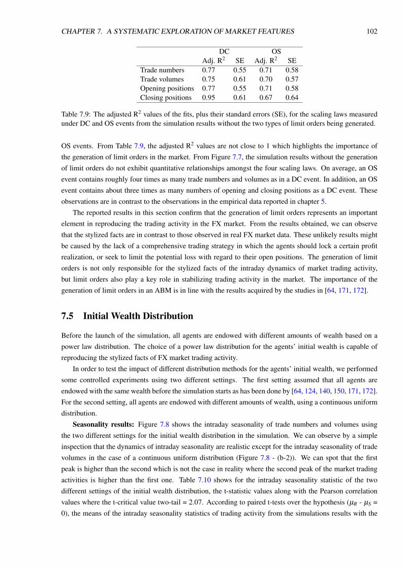
CHAPTER 7. A SYSTEMATIC EXPLORATION OF MARKET FEATURES 102
DC OSAdj. R2 SE Adj. R2 SE
Trade numbers 0.77 0.55 0.71 0.58Trade volumes 0.75 0.61 0.70 0.57Opening positions 0.77 0.55 0.71 0.58Closing positions 0.95 0.61 0.67 0.64
Table 7.9: The adjusted R2 values of the fits, plus their standard errors (SE), for the scaling laws measuredunder DC and OS events from the simulation results without the two types of limit orders being generated.
OS events. From Table 7.9, the adjusted R2 values are not close to 1 which highlights the importance of
the generation of limit orders in the market. From Figure 7.7, the simulation results without the generation
of limit orders do not exhibit quantitative relationships amongst the four scaling laws. On average, an OS
event contains roughly four times as many trade numbers and volumes as in a DC event. In addition, an OS
event contains about three times as many numbers of opening and closing positions as a DC event. These
observations are in contrast to the observations in the empirical data reported in chapter 5.
The reported results in this section confirm that the generation of limit orders represents an important
element in reproducing the trading activity in the FX market. From the results obtained, we can observe
that the stylized facts are in contrast to those observed in real FX market data. These unlikely results might
be caused by the lack of a comprehensive trading strategy in which the agents should lock a certain profit
realization, or seek to limit the potential loss with regard to their open positions. The generation of limit
orders is not only responsible for the stylized facts of the intraday dynamics of market trading activity,
but limit orders also play a key role in stabilizing trading activity in the market. The importance of the
generation of limit orders in an ABM is in line with the results acquired by the studies in [64, 171, 172].
7.5 Initial Wealth Distribution
Before the launch of the simulation, all agents are endowed with different amounts of wealth based on a
power law distribution. The choice of a power law distribution for the agents’ initial wealth is capable of
reproducing the stylized facts of FX market trading activity.
In order to test the impact of different distribution methods for the agents’ initial wealth, we performed
some controlled experiments using two different settings. The first setting assumed that all agents are
endowed with the same wealth before the simulation starts as has been done by [64, 124, 140, 150, 171, 172].
For the second setting, all agents are endowed with different amounts of wealth, using a continuous uniform
distribution.
Seasonality results: Figure 7.8 shows the intraday seasonality of trade numbers and volumes using
the two different settings for the initial wealth distribution in the simulation. We can observe by a simple
inspection that the dynamics of intraday seasonality are realistic except for the intraday seasonality of trade
volumes in the case of a continuous uniform distribution (Figure 7.8 - (b-2)). We can spot that the first
peak is higher than the second which is not the case in reality where the second peak of the market trading
activities is higher than the first one. Table 7.10 shows for the intraday seasonality statistic of the two
different settings of the initial wealth distribution, the t-statistic values along with the Pearson correlation
values where the t-critical value two-tail = 2.07. According to paired t-tests over the hypothesis (µR - µS =
0), the means of the intraday seasonality statistics of trading activity from the simulations results with the

CHAPTER 7. A SYSTEMATIC EXPLORATION OF MARKET FEATURES 103
Figure 7.8: The intraday seasonality of trade (a) numbers and (b) volumes from the simulation results whereall agents are endowed with (1) the same wealth and (2) different amounts of wealth, using a continuousuniform distribution.
(a) (b)tsv corr tsv corr
Trade numbers -1.06E-09 + 0.98 -8.07E-09 + 0.98Trade volumes 3.38E-16 + 0.98 4.47E-10 + 0.98Opening positions 3.33E-09 + 0.98 -4.06E-09 + 0.98Closing positions 1.44E-09 + 0.98 -3.09E-09 + 0.98
Table 7.10: T-statistic (tsv) values and Pearson correlation (corr) values where the t-critical value two-tail= 2.07 - Intraday seasonality statistic from the simulation results where all agents are endowed with (a) thesame wealth and (b) different amounts of wealth, using a continuous uniform distribution.
two different settings of the initial wealth distribution are roughly equivalent to those for the real FX market,
with 95% confidence level.
Correlation results: Table 7.11 reports the correlation coefficients of the different market trading activ-
ities from the simulation results with different settings for the initial wealth distribution. The type of initial
wealth distribution does not affect the correlation between the different market trading activities. Neverthe-
less, such a parameter greatly affects the correlation between intraday price volatility and market trading
activity. Consequently, it would appear that the correlation between price volatility and market trading ac-
tivity depends basically on those agents at the launch of the simulation who possess different wealth by
means of a power law distribution.
Scaling laws results: For the two different settings of the initial wealth distribution, the four scaling
(a) (b)Trade numbers and volumes + 0.95 + 0.90Numbers of buy and sell executed order + 0.99 + 0.99Numbers of opening and closing positions + 0.99 + 0.98Intraday price volatilities and trader numbers + 0.01 - 0.01Intraday price volatilities and volumes - 0.02 - 0.03
Table 7.11: Correlation coefficients computed for the EUR/USD trading activity from the simulation re-sults where all agents are endowed with (a) the same wealth and (b) different amounts of wealth, using acontinuous uniform distribution.

CHAPTER 7. A SYSTEMATIC EXPLORATION OF MARKET FEATURES 104
Figure 7.9: Scaling laws are plotted from the simulation results where all agents are endowed with (a) thesame wealth and (b) different amounts of wealth, using a continuous uniform distribution. The x-axis showsthe price moves thresholds of the EUR/USD observations.
laws are not exhibited in the simulation results (as shown from Figure 7.9 and Table 7.12). Table 7.12
reports, for the two different settings of initial wealth distribution, the adjusted R2 values of the fits, plus
their standard errors, for the four scaling laws measured under DC and OS events. From Table 7.12, it is
clear that the adjusted R2 values are not very close to 1, which implies an insignificant fit. From Figure
7.9, the simulation results in the case of the distribution of agents’ initial wealth is based on a continuous
uniform distribution, do not exhibit the quantitative relationships of the trade volumes’ scaling law. On
average, an OS event contains roughly three times as many trade volumes as a DC event, which is contrary
to the observations in the empirical data where, on average, an OS event contains roughly twice as many
trade volumes as a DC event.
Assuming that all agents start with the same wealth in the market does not affect the seasonality statisti-
cal properties of the different market trading activities. However, it affects the correlation between intraday
price volatility and trade numbers and volumes. Also, such an assumption has an impact on the exhibition
of scaling laws properties of market trading activities. One of the reasons behind these results is that real
markets involve heterogeneity in terms of the wealth distribution of the traders. Accordingly, we would
argue that the assumption that agents possess the same wealth at the beginning of the market as has been
done by [64, 124, 140, 150, 171, 172], is not the way forward in this field.
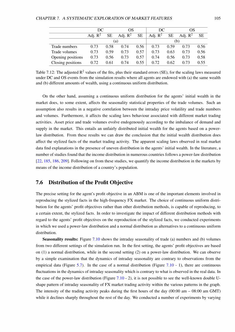
CHAPTER 7. A SYSTEMATIC EXPLORATION OF MARKET FEATURES 105
DC OS DC OSAdj. R2 SE Adj. R2 SE Adj. R2 SE Adj. R2 SE
(a) (b)Trade numbers 0.73 0.58 0.74 0.56 0.73 0.59 0.73 0.56Trade volumes 0.73 0.59 0.73 0.57 0.73 0.63 0.73 0.56Opening positions 0.73 0.56 0.73 0.57 0.74 0.56 0.73 0.58Closing positions 0.72 0.61 0.74 0.55 0.72 0.62 0.73 0.55
Table 7.12: The adjusted R2 values of the fits, plus their standard errors (SE), for the scaling laws measuredunder DC and OS events from the simulation results where all agents are endowed with (a) the same wealthand (b) different amounts of wealth, using a continuous uniform distribution.
On the other hand, assuming a continuous uniform distribution for the agents’ initial wealth in the
market does, to some extent, affects the seasonality statistical properties of the trade volumes. Such an
assumption also results in a negative correlation between the intraday price volatility and trade numbers
and volumes. Furthermore, it affects the scaling laws behaviour associated with different market trading
activities. Asset price and trade volumes evolve endogenously according to the imbalance of demand and
supply in the market. This entails an unfairly distributed initial wealth for the agents based on a power-
law distribution. From these results we can draw the conclusion that the initial wealth distribution does
affect the stylized facts of the market trading activity. The apparent scaling laws observed in real market
data find explanations in the presence of uneven distribution in the agents’ initial wealth. In the literature, a
number of studies found that the income distribution in numerous countries follows a power-law distribution
[22, 185, 186, 209]. Following on from these studies, we quantify the income distribution in the markets by
means of the income distribution of a country’s population.
7.6 Distribution of the Profit Objective
The precise setting for the agent’s profit objective in an ABM is one of the important elements involved in
reproducing the stylized facts in the high-frequency FX market. The choice of continuous uniform distri-
bution for the agents’ profit objectives rather than other distribution methods, is capable of reproducing, to
a certain extent, the stylized facts. In order to investigate the impact of different distribution methods with
regard to the agents’ profit objectives on the reproduction of the stylized facts, we conducted experiments
in which we used a power-law distribution and a normal distribution as alternatives to a continuous uniform
distribution.
Seasonality results: Figure 7.10 shows the intraday seasonality of trade (a) numbers and (b) volumes
from two different settings of the simulation run. In the first setting, the agents’ profit objectives are based
on (1) a normal distribution, while in the second setting (2) on a power-law distribution. We can observe
by a simple examination that the dynamics of intraday seasonality are contrary to observations from the
empirical data (Figure 5.7). In the case of a normal distribution (Figure 7.10 - 1), there are continuous
fluctuations in the dynamics of intraday seasonality which is contrary to what is observed in the real data. In
the case of the power-law distribution (Figure 7.10 - 2), it is not possible to see the well-known double U-
shape pattern of intraday seasonality of FX market trading activity within the various patterns in the graph.
The intensity of the trading activity peaks during the first hours of the day (00:00 am – 08:00 am GMT)
while it declines sharply throughout the rest of the day. We conducted a number of experiments by varying

CHAPTER 7. A SYSTEMATIC EXPLORATION OF MARKET FEATURES 106
Figure 7.10: The intraday seasonality of trade (a) numbers and (b) volumes from two different settings of thesimulation run for the distribution of the agents’ profit objectives: (1) a normal distribution; (2) a power-lawdistribution.
(a) (b)tsv corr tsv corr
Trade numbers -2.03E-10 + 0.81 -6.05E-11 - 0.08Trade volumes 2.63E-16 + 0.83 -2.02E-10 - 0.02Opening positions -1.03E-10 + 0.65 -5.05E-11 - 0.11Closing positions 2.06E-10 + 0.82 6.06E-11 - 0.09
Table 7.13: T-statistic (tsv) values and Pearson correlation (corr) values, where the t-critical value two-tail= 2.07 - Intraday seasonality statistic for two different settings of the simulation for the distribution of theagents’ profit objectives: (a) a normal distribution; (b) a power-law distribution.
the scaling exponent of the power law distribution, but this did not change these unrealistic results.
Table 7.13 shows the t-statistic values along with the Pearson correlation values, where the t-critical
value two-tail = 2.07, for the intraday seasonality statistic for the different settings of the agents’ profit
objectives distribution. According to paired t-tests with regard to the hypothesis (µR - µS = 0), the means
of the intraday seasonality statistics of trading activity from the simulations’ results, using different settings
of the profit objectives distribution, are roughly equivalent to those for the real FX market, with a 95%
confidence level. However, in the case of the power law distribution, the correlations between the seasonality
statistics of real data and simulation data are negative.
Correlation results: Table 7.14 reports the correlation coefficients of the different market trading ac-
tivities from the simulation results with different settings of the agents’ profit objective distribution. The
(a) (b)Trade numbers and volumes + 0.98 + 0.98Numbers of buy and sell executed order + 0.57 + 0.60Numbers of opening and closing positions + 0.25 + 0.31Intraday price volatilities and trader numbers - 0.003 -0.01Intraday price volatilities and volumes -0.0004 + 0.01
Table 7.14: Correlation coefficients computed for the different EUR/USD trading activity for two differentsettings of the simulation run for the distribution of the agents’ profit objectives: (a) a normal distribution;(b) a power-law distribution.

CHAPTER 7. A SYSTEMATIC EXPLORATION OF MARKET FEATURES 107
Figure 7.11: Scaling laws are plotted from two different settings of the simulation run for the distributionmethod for the agents’ profit objectives: (a) a normal distribution; (b) a power-law distribution. The x-axisshows the price moves thresholds of the EUR/USD observations.
distribution method in terms of agents’ profit objectives does not affect the correlation between the trade
numbers and volumes. But the distribution method affects the correlation between (a) the numbers of buy
and sell executed orders, and (b) the numbers of opening and closing positions. In addition, such a distribu-
tion method affects the correlation between intraday price volatility and market trading activity considerably.
Scaling laws results: For the different settings of the agents’ profit objective distribution, the four
scaling laws and the six quantitative relationships amongst them are not exhibited in the simulation results
(as shown from Figure 7.11 and Table 7.15). Table 7.15 reports the adjusted R2 values of the fits, plus their
standard errors, for the four scaling laws measured under DC and OS events. It is clear that the adjusted R2
values are not very close to 1, which implies an insignificant fit.
The reported results in this section emphasise that the price dynamics in the market are a result of
the existence of heterogeneous expectations amongst traders. According to [19] “One of the things that
microeconomics teaches you is that individuals are not alike. There is heterogeneity, and probably the most
important heterogeneity here is heterogeneity of expectations. If we didn’t have heterogeneity, there would
be no trade. But developing an analytic model with heterogeneous agents is difficult.” (p. 301).

CHAPTER 7. A SYSTEMATIC EXPLORATION OF MARKET FEATURES 108
DC OS DC OSAdj. R2 SE Adj. R2 SE Adj. R2 SE Adj. R2 SE
(a) (b)Trade numbers 0.80 0.58 0.71 0.58 0.84 0.50 0.69 0.60Trade volumes 0.80 0.58 0.71 0.58 0.84 0.49 0.69 0.60Opening positions 0.73 0.70 0.73 0.55 0.80 0.57 0.69 0.59Closing positions 0.94 0.29 0.69 0.61 0.98 0.15 0.69 0.62
Table 7.15: The adjusted R2 values of the fits, plus their standard errors (SE), for the scaling laws measuredunder DC and OS events from two different settings of the simulation run for the distribution method for theagents’ profit objectives: (a) a normal distribution; (b) a power-law distribution.
The power-law and the normal distribution characterize inadequately distributed profit objective values.
Consequently, this results in a large group of agents having similar behaviour patterns and preferences
whereas, in reality, traders have a variety of preferences and demands. For this reason, choosing a continuous
uniform distribution is a good option, given that it provides an equal distribution with a variety of profit
objective values for the trading agents.
7.7 Risk Appetites
The risk appetite parameter is used to model the cautiousness and aggressiveness of agents with regard to
trading. From the microscopic analysis of the OANDA individual traders’ historical transactions, we found
on average, that the traders’ risk appetites are higher than their profit objectives (as explained in section
6.5.4). Accordingly, in our ABFXM, we defined the agents’ risk appetites to be four times that of their
profit objectives.
To test the impact of such an element on reproducing the stylized facts, we varied the risk appetites’
parameter in the simulation. Although we have conducted a number of experiments, we report the results of
four indicative cases in which the agents’ risk appetites relate to their profit objectives as follows.
1. High-risk: a trading strategy involves high risk when the agent’s risk appetite is four times that of its
profit objective. The high risk appetite setting is the one used in our ABFXM.
2. Low-risk: the agent’s risk appetite is equal to the agent’s profit objective.
3. Zero-risk: an agent will close its open position once the unrealized losses for the position fall below
zero, which means that the position is in loss.
4. A combination of the three levels of risk.
Seasonality results: Figure 7.12 shows the intraday seasonality of trade numbers and volumes from the
four different simulation outcomes as per the four cases above. When the agents’ trading strategy involves
high risk, the patterns of intraday seasonality of trade numbers are exhibited (this is the default setting of
the simulation). Meanwhile, when the agents’ trading strategy involves (b) low risk, (c) zero risk or (d) a
combination of the three levels of risk, the patterns of intraday seasonality of trade numbers move within
a narrow level of the resistance, whereas in reality it is wider. The level of the agents’ risk appetites does
not affect the intraday seasonality of trade volumes. Table 7.16 shows for the intraday seasonality statistic
of different settings of the agents’ risk appetites, the t-statistic values, along with the Pearson correlation

CHAPTER 7. A SYSTEMATIC EXPLORATION OF MARKET FEATURES 109
Figure 7.12: The intraday seasonality of trade numbers and volumes from four different simulation results,where the agents’ risk appetites involve (a) high-risk, (b) low-risk, (c) zero-risk or (d) a combination of thethree levels of risk.
(a) (b) (c) (d)tsv corr tsv corr tsv corr tsv corr
Trade numbers 2.03E-10 + 0.90 -5.07E-10 + 0.98 -1.07E-09 + 0.98 -7.82E-10 + 0.97Trade volumes 1.11E-10 + 0.86 -1.01E-15 + 0.98 5.15E-10 + 0.98 -9.99E-10 + 0.98Opening positions 2.02E-10 + 0.91 -8.05E-10 + 0.98 7.21E-10 + 0.99 -8.08E-10 + 0.98Closing positions -6.08E-10 + 0.91 8.48E-10 + 0.98 3.28E-10 + 0.98 2.50E-10 + 0.96
Table 7.16: T-statistic (tsv) values and Pearson correlation (corr) values, where the t-critical value two-tail =2.07 - Intraday seasonality statistic from four different simulation results, in which the agents’ risk appetitesinvolve (a) high-risk, (b) low-risk, (c) zero-risk or (d) a combination of the three levels of risk.
values. According to the paired t-tests with regard to the hypothesis (µR - µS = 0), the means of the intraday
seasonality statistics of trading activity from the simulation outcomes with different risk appetite settings,
are roughly equivalent to those of the real FX market, with a 95% confidence level.
Correlation results: Looking at Table 7.17, the agents’ risk appetites do not affect the correlation
between (i) trade numbers and volumes, (ii) the number of buy and sell orders and (iii) the number of
opening and closing positions. However, the risk appetite results in a negative correlation between the
intraday price volatilities and trade numbers and volumes when the risk is low/zero or there is a mixture of
risk appetites in the agent population.
Scaling laws results: The scaling laws are not exhibited when the risk is low/zero or there is a mixture
of risk appetites in the agent population. This is also clear from Table 7.18 as the adjusted R2 values for the
three different settings of the agents’ risk appetites parameter (b, c, d) are not close to 1, which means an
insignificant fit.

CHAPTER 7. A SYSTEMATIC EXPLORATION OF MARKET FEATURES 110
(a) (b) (c) (d)Trade numbers and volumes + 0.92 + 0.87 + 0.89 + 0.90Numbers of buy and sell executed order + 0.99 + 0.99 + 0.99 + 0.99Numbers of opening and closing positions + 0.98 + 0.99 + 0.99 + 0.99Intraday price volatilities and trader numbers + 0.46 - 0.02 - 0.04 - 0.02Intraday price volatilities and volumes + 0.31 - 0.05 - 0.06 - 0.05
Table 7.17: Correlation coefficients computed for the different EUR/USD trading activity from four differentsimulation results, in which the agents’ risk appetites involve (a) high-risk, (b) low-risk, (c) zero-risk or (d)a combination of the three levels of risk.
Figure 7.13: Scaling laws are plotted from four different settings of the simulation run in which the agents’risk appetites involve (a) high-risk, (b) low-risk, (c) zero-risk or (d) a combination of the three levels of risk.The x-axis shows the price moves thresholds of the EUR/USD observations.

CHAPTER 7. A SYSTEMATIC EXPLORATION OF MARKET FEATURES 111
DC OS DC OSAdj. R2 SE Adj. R2 SE Adj. R2 SE Adj. R2 SE
(a) (b)Trade numbers 0.91 0.37 0.90 0.31 0.74 0.56 0.73 0.58Trade volumes 0.94 0.35 0.94 0.31 0.72 0.63 0.72 0.56Opening positions 0.92 0.35 0.93 0.31 0.74 0.56 0.73 0.60Closing positions 0.91 0.39 0.90 0.35 0.74 0.56 0.73 0.58
(c) (d)Trade numbers 0.73 0.57 0.73 0.58 0.74 0.56 0.73 0.58Trade volumes 0.72 0.66 0.72 0.55 0.73 0.58 0.73 0.57Opening positions 0.74 0.56 0.73 0.58 0.74 0.56 0.73 0.58Closing positions 0.73 0.59 0.73 0.60 0.74 0.56 0.73 0.58
Table 7.18: The adjusted R2 values of the fits, plus their standard errors (SE), for the scaling laws measuredunder DC and OS events from four different settings of the simulation run in which the agents’ risk appetitesinvolve (a) high-risk, (b) low-risk, (c) zero-risk or (d) a combination of the three levels of risk.
Return on Investment (ROI): From the simulation results, we measure the agents’ performance over
a period of one simulated month by means of their return on investment (ROI). The aim is to evaluate the
efficiency of their investments in terms of four different settings of trading risk: (a) high-risk, (b) low-risk,
(c) zero-risk or (d) a combination of the three levels of risk. ROI can either be positive or negative, which
means that the return can either mean a profit or a loss. To measure an agent’s return on investment, the
total return of an agent’s transactions over a period T is divided by the agent’s initial investment. The result
is expressed as a percentage, and is defined by:
ROI =(∑n
i=1 ri− yi)
w(7.1)
where n is the total number of transactions during the period T, y is the ith transaction, ri is the return
from the ith transaction, yi is the investment cost of the ith transaction, and w is the agent’s initial investment.
Table 7.19 reports some of the basic descriptive statistics of the agents’ ROI from four independent runs
of the simulation. In terms of the profit factor, we can see that the maximum agent’s ROI occurs when the
agent’s trading strategy is a high-risk one. In addition, in the case of high-risk, the average ROI is positive,
while for the other three settings the average ROI is negative. This result indicates a better performance when
the agent’s risk appetite involves high-risk activity. In the case of zero-risk, 99.21% of the agents achieve
losses, while only 0.79% of agents achieve profits. Alternatively, we can see the reasonable percentage
values of the winning and losing agents when their risk appetite is high or low, indicating the importance of
involving risk in the trading strategy. The results show that being able to take high risks is closely linked
with generating high profits. It is difficult to evaluate precisely the traders’ ROI due to the lack of knowledge
and data about the real traders’ ROI.
The level of the agent’s risk appetite is considered to be an essential element in an ABM. In our agent-
based models of traders, an agent’s risk appetite is articulated in terms of the agent’s profit objective. We
found that setting a high level of agents’ risk appetites compared to the agents’ profit objectives means that
the ABFXM is capable of reproducing, to a certain extent, the trading activity in the market. However,
having the agent’s risk appetite higher than four times their profit objectives, results in negative correlations
between the intraday price volatilities and trade numbers (- 0.02) and volumes (- 0.03). This is because of
the implications of high risk activity on an agent’s wealth performance, which triggers margin calls. The

CHAPTER 7. A SYSTEMATIC EXPLORATION OF MARKET FEATURES 112
Statistics (a) (b) (c) (d)Max 3693.68 % 964.23 % 79.70 % 88.32 %Min -100 % -100 % -100 % - 100 %Mean 13.13 % -1.53 % -10.10 % -10.60 %Std. Dev 1.24 0.82 0.23 0.22Winning agents (%) 44.90% 38.76% 0.79% 0.60 %Losing agents (%) 55.10% 61.24% 99.21% 99.40 %
Table 7.19: Basic descriptive statistics of the agents’ ROI from four independent runs of the simulation inwhich the agents’ risk appetites involve (a) high-risk, (b) low-risk, (c) zero-risk or (d) a combination of thethree levels of risk.
right setting of the agents’ risk appetites parameter significantly affects the correlation between intraday
price volatility and market trading activities. In particular, using a low risk appetite results in a negative
correlation between intraday price volatility and market trading activities. Such a negative correlation may
be affected by the high intensity of trading activities when the price collapses. Accordingly, the correlation
results confirm what has been observed in market data: traders in the high-frequency market tend to hold
losing positions for a long period of time.
7.8 Contrarian and Trend-Following Strategies
In our ABFXM, we consider a population whose trading strategies are organized into two major classes
with equal number of agents: trend-following and contrary ZI-DCT0 trading strategies. We aim to study the
impact of using just one of these strategies for the entire population and hence we conducted experiments
where the adopted trading strategy in the market was either the trend-following or the contrary strategy.
Also, we examined the effect of the existence of different percentages of contrary agents in comparison
to trend-following agents on the exhibition of the stylized facts. Based on the results obtained, the exami-
nation can be divided into two cases, with each case involving a series of experiments. In the first case, the
number of contrary agents is between 30% - 70% of the total population. In the second case, the number
of contrary agents is more than (i) 70% or (ii) less than 30% of the total population: these two sub cases
generate very similar results due to a very large number of agents having the same trading strategy. Hence,
we only present an example of the latter in this section due to the similarity of the results and for brevity.
In addition, a series of experiments were conducted to study the impact of the inclusion of random trades
in the market; random trades have been incorporated in the ABFXM to emulate the fact that in reality traders
take decisions influenced by exogeneous to the market events.
Seasonality results: Figure 7.14 shows the intraday seasonality of trade numbers from the ABFXM
populated with (a) just contrary agents, (b) just trend-followers agents, (c) a mixture of 40% contrary and
60% trend-followers agents, (d) a mixture of 70% contrary and 30% trend-followers agents and (e) exclusive
of random trades from the agents’ trading strategy. The dynamics of intraday seasonality of trade numbers
resemble those observed in the empirical data where the double U-shape pattern is exhibited. However, in
the case (d) the ABFXM populated with a mixture of a mixture of 70% contrary and 30% trend-followers
agents, the patterns of intraday seasonality move within a narrow level of the resistance, while in the real
data they are wider. This may possibly be due to the imbalance of orders generated by the agents in the
market. According to the results reported in Table 7.20 for the paired t-test, the means of the intraday
seasonality statistics of trading activity from the simulation outcomes, are roughly equivalent to those of the

CHAPTER 7. A SYSTEMATIC EXPLORATION OF MARKET FEATURES 113
Figure 7.14: The intraday seasonality of trade numbers where the ABFXM populated with (a) just contraryagents, (b) just trend-followers agents, (c) a mixture of 40% contrary and 60% trend-followers agents, (d) amixture of 70% contrary and 30% trend-followers agents and (e) exclusive random trades.
real FX market, with a 95% confidence level.
Correlation results: From Table 7.21, we can observe that the adoption of single strategies does not
affect the correlation between trade numbers and volumes, number of buy and sell orders and number of
opening and closing positions. However, it results in a negative correlation between the intraday price
volatilities and trade numbers and volumes. This implies that the price behaviour in the market is the result
of a balance of various trading strategies and levels of activity. The same is the case when random trades
are excluded: although there is no impact on the correlation between various trading quantities, the intraday
price volatilities and trade numbers/volumes are affected.
Scaling laws results: When either of the strategies is adopted by the whole population and when random
trades are excluded, then the scaling laws are not exhibited in the simulation results. The results in Table
7.22 show that the adjusted R2 values are not close to 1, which entails an insignificant fit. Also, the estimated
standard errors are higher than the estimated errors for scaling law relationships observed in the empirical
data. The results of case (c) the ABFXM populated with a mixture of 40% contrary and 60% trend-followers
agents, exhibit, the full set of the FX market trading activity stylized facts.
In our ABFXM, we limit the trading strategies to two classes of trend-following and contrary trading
strategies, in which agents can enter or leave the market, depending on the price behaviour. This is an ex-
treme simplification with regards to modelling the market traders’ behaviour. The results from our ABFXM
show that the simplification in the two classes of trading strategies is enough to achieve an understanding,
to a certain extent, of the original market trading activity stylized facts. However, the possibility of a wider
class of trading strategies in an ABFXM, and the traders’ decisions on the basis of previous performance,
is without doubt an interesting area with regard to future exploration. The problem, in this respect, is that

CHAPTER 7. A SYSTEMATIC EXPLORATION OF MARKET FEATURES 114
(a) (b) (c)tsv corr tsv corr tsv corr
Trade numbers 1.36E-09 + 0.99 -1.76E-09 + 0.99 -4.92E-09 + 0.99Trade volumes 4.32E-05 + 0.99 -6.06E-05 + 0.99 5.67E-10 + 0.99
Opening positions 1.35E-09 + 0.99 -1.70E-09 + 0.99 -4.92E-09 + 0.99Closing positions 1.34E-09 + 0.99 -1.72E-09 + 0.99 -4.90E-09 + 0.99
(d) (e)tsv corr tsv corr
Trade numbers -1.23E-16 + 0.98 1.74E-09 + 0.99Trade volumes 7.20E-10 + 0.98 -1.59E-05 + 0.99
Opening positions -1.21E-16 + 0.99 1.72E-09 + 0.99Closing positions -1.21E-16 + 0.98 1.72E-09 + 0.99
Table 7.20: T-statistic (tsv) and Pearson correlation (corr) values, where the ABFXM populated with (a)just contrary agents, (b) just trend-followers agents, (c) a mixture of 40% contrary and 60% trend-followersagents, (d) a mixture of 70% contrary and 30% trend-followers agents and (e) exclusive random trades.
(a) (b) (c) (d) (e)Trade numbers and volumes + 0.92 + 0.94 + 0.95 + 0.88 + 0.91Numbers of buy and sell order + 0.96 + 0.99 + 0.99 + 1 + 0.99Numbers of opening and closing positions + 0.96 + 0.98 + 0.98 + 1 + 0.98Intraday price volatilities and trader numbers - 0.01 - 0.03 + 0.39 - 0.03 - 0.01Intraday price volatilities and volumes - 0.03 - 0.02 + 0.26 - 0.10 - 0.05
Table 7.21: Correlation coefficients computed for the EUR/USD trading activity where the ABFXM popu-lated with (a) just contrary agents, (b) just trend-followers agents, (c) a mixture of 40% contrary and 60%trend-followers agents, (d) a mixture of 70% contrary and 30% trend-followers agents and (e) exclusiverandom trades.
DC OS DC OS DC OSR2 SE R2 SE R2 SE R2 SE R2 SE R2 SE
(a) (b) (c)Trade numbers 0.73 0.59 0.73 0.58 0.73 0.59 0.73 0.57 0.97 0.35 0.95 0.36Trade volumes 0.73 0.62 0.73 0.56 0.74 0.60 0.72 0.57 0.97 0.35 0.95 0.36Opening positions 0.74 0.56 0.73 0.58 0.74 0.56 0.74 0.58 0.97 0.35 0.95 0.37Closing positions 0.72 0.62 0.73 0.56 0.72 0.62 0.73 0.56 0.97 0.36 0.95 0.36
DC OS DC OSR2 SE R2 SE R2 SE R2 SE
(d) (e)Trade numbers 0.73 0.59 0.73 0.57 0.73 0.59 0.73 0.56Trade volumes 0.74 0.61 0.72 0.57 0.74 0.62 0.72 0.57Opening positions 0.73 0.59 0.73 0.59 0.74 0.56 0.73 0.58Closing positions 0.73 0.61 0.73 0.58 0.71 0.63 0.74 0.55
Table 7.22: The adjusted R2 values of the fits, plus their standard errors (SE), for the scaling laws measuredunder DC and OS events where the ABFXM populated with (a) just contrary agents, (b) just trend-followersagents, (c) a mixture of 40% contrary and 60% trend-followers agents, (d) a mixture of 70% contrary and30% trend-followers agents and (e) exclusive random trades.

CHAPTER 7. A SYSTEMATIC EXPLORATION OF MARKET FEATURES 115
Figure 7.15: Scaling laws are plotted where the ABFXM populated with (a) just contrary agents, (b) justtrend-followers agents, (c) a mixture of 40% contrary and 60% trend-followers agents, (d) a mixture of 70%contrary and 30% trend-followers agents and (e) exclusive random trades. The x-axis shows the price movesthresholds of the EUR/USD observations.

CHAPTER 7. A SYSTEMATIC EXPLORATION OF MARKET FEATURES 116
the analysis and exploration of trading activities in the ABFXM can become highly misleading and difficult
to study, because the broader class of trading strategies may produce a source of complexity for the market
analysis.
Therefore, the results support that competition between trend-follower agents and contrary agents would
have a tendency to stabilize the market. The key role played by the coexistence of such agents’ trading
strategies is one of the main elements responsible for exhibiting stylized facts in an ABFXM. Random
trading governs the likelihood of the agents changing their trading strategy, and it is a vital element of the
model. In any case, the intraday seasonality statistics of the different market trading activities are exhibited
in the limit where the agents’ population is composed only of trend-followers or only by contrary traders,
even without random trades taking place. Therefore, these simple experiments show us which stylized
facts depend critically on the interaction between different trading strategies. The generalized scaling law
properties and the correlation behaviour results appear to be sensitive to the heterogeneity of agent trading
strategies.
Similar studies by [5–7] showed that the stylized facts are exhibited in an ABM by introducing the
possibility of the agents to enter or leave the market depending on the behaviour of the price. The mechanism
to enter or leave the market is linked to the existence of a threshold that the agents use to decide to operate
in the market by comparing the threshold with the price movement.
7.9 Trading Time Window
Although the FX market operates 24 hours a day and does not have fixed trading time windows as the stock
market, the worldwide FX market centres’ business hours have a significant effect on characterizing the
daily flow of the market’s activity. The intensity of trading activity increases during the opening hours of the
FX market centres in the morning, whereas it decreases during the closing hours. The overlapping business
hours of two or more FX market centres witnesses a high level of trading activity compared to the other
times.
Initially, we decided to model the agents without incorporating the role of FX market trading sessions
and holidays. The motivation behind our decision was to account for the significant impact of algorithmic
trading. Algorithmic trading, also referred to as automated trading, uses computer programs to place orders
automatically which may be outside a trader’s normal business hours. It has attracted many FX traders and,
most importantly, is one of the reasons for the growth of the FX market. However, not modelling business
hours has a significant impact on the emergence stylized facts.
Seasonality results: Figure 7.16 shows the intraday seasonality of trade numbers from the simulation
results, without incorporating the role of FX market trading sessions. By a simple examination, we can
clearly see that the intraday seasonality of FX market trading activity is not exhibited as it is not possible to
spot the double U-shape pattern. This is for the following reasons: the highest volume of trading activity
takes place in the first hour of the day, as well as around 08:00 GMT. The trading activity declines sharply
from around 09:00 GMT and continues throughout the day, which does not reflect reality. In reality, the
daily trading activity increases between 08:00 – 09:00 GMT mirroring the opening hours of the London
trading session, and peaks when London and New York trading sessions overlap around 13:00 – 16:00 GMT.
According to the results reported in Table 7.23 for the paired t-test, the means of the seasonality statistics of
the FX market trading activity are roughly the same to the simulation results, without incorporating the role

CHAPTER 7. A SYSTEMATIC EXPLORATION OF MARKET FEATURES 117
Figure 7.16: Intraday seasonality of trade numbers from the simulation results, without incorporating therole of FX market trading sessions.
tsv corrTrade numbers -3.02E-10 + 0.05Trade volumes 4.64E-10 + 0.02Number of opening positions -3.05E-10 + 0.05Number of closing positions -3.05E-09 + 0.04
Table 7.23: T-statistic (tsv) values and Pearson correlation (corr) values, where the t-critical value two-tail= 2.07 - Intraday seasonality statistic from simulation results without incorporating the role of FX markettrading sessions.
of FX market trading sessions. Nevertheless, the correlations between the seasonality statistics of real data
and simulation data are extremely low. The correlation results indicate the significant role of incorporating
the FX market trading sessions in an agent-based model of FX trading.
Correlation results: Table 7.24 reports the correlation coefficients of the different market trading activi-
ties from the simulation results, without incorporating the role of FX market trading sessions. The inclusion
of the role of FX market trading sessions does not affect the correlation between (a) trade numbers and
volumes, (b) numbers of buy and sell executed orders and (c) numbers of opening and closing positions.
However, it affects extensively the correlation between the intraday price volatilities and trade numbers
and volumes. This means that the time periods of high market trading activity are also the time periods
associated with large price volatilities.
Scaling laws results: The four scaling laws measured under DC events are not exhibited in the simu-
Correlation coefficientTrade numbers and volumes + 0.87Numbers of buy and sell executed order + 0.99Numbers of opening and closing positions + 0.98Intraday price volatilities and trader numbers + 0.002Intraday price volatilities and volumes - 0.09
Table 7.24: Correlation coefficients computed for the different EUR/USD trading activity from the simula-tion results without incorporating the role of FX market trading sessions.

CHAPTER 7. A SYSTEMATIC EXPLORATION OF MARKET FEATURES 118
Figure 7.17: Scaling laws are plotted from the simulation results without incorporating the role of FX markettrading sessions. The x-axis shows the price moves thresholds of the EUR/USD observations.
DC OSAdj. R2 SE Adj. R2 SE
Trade numbers 0.73 0.62 0.99 0.09Trade volumes 0.75 0.60 0.72 3.50Number of opening positions 0.74 0.61 0.99 0.58Number of closing positions 0.72 0.63 0.99 0.11
Table 7.25: The adjusted R2 values of the fits, plus their standard errors (SE), for the scaling laws measuredunder DC and OS events from the simulation results without incorporating the role of FX market tradingsessions.
lation results when the FX market trading sessions in the agents’ trading time window are not incorporated
(as shown from Figure 7.17 and Table 7.25). In addition, the trade volumes scaling law measured under OS
events is not exhibited in the simulation results. Table 7.25 reports the adjusted R2 values of the fits, plus
their standard errors, for the four scaling laws measured under DC and OS events. It is clear the adjusted R2
values are not very close to 1, which implies an insignificant fit.
The results reported in this section stress the importance of incorporating the role of the FX market
trading sessions in modelling the agents trading time window. The behaviour of market trading activity
exhibits a periodic pattern called seasonal. The seasonal patterns are evidently correlated with the changing
presence of the main worldwide FX market centres. The results present evidence of a strong correlation
between market trading activity and the time of day.
The correlation between market activity and volatility requires us to model a heterogeneous trading time
window with the help of information related to the main worldwide FX market centres’ business trading
hours. The time zones and the typical business hours of the FX market trading sessions (e.g., London, New
York, Tokyo) are well known. The results demonstrate the importance of daily seasonal patterns of trading
activity in the generation of scaling law properties.

CHAPTER 7. A SYSTEMATIC EXPLORATION OF MARKET FEATURES 119
7.10 Order Size
The order size parameter is a very important element with regard to any ABM as the order size is associated
with changes in the agent’s wealth. In the ABM literature, there are two main approaches for characterizing
the order size placed by an agent in an ABM, which are: the direct approach involves an agent placing an
order in which the order size is proportional to the agent’s wealth. This approach was adopted by a number
of models including [120]. The second approach uses a constant trading proportion parameter that controls
the size of an agent’s order in terms of the agent’s wealth. In other words, depending on the value of the
trading proportion parameter, an agent buys/sells quantities of an asset proportional to its current wealth.
Thus, only a fraction x of the agent’s cash is invested. The trading proportion is defined before the launch
of the simulation. Examples of ABMs using this approach are [137, 171, 172, 188].
In this section, we examine the impact of these two approaches on the behaviour of the market trading
activity. With regard to the second approach, we performed several experiments in which we scaled the
trading proportion parameters from 10% to 90%. For brevity, and since for some of the results the changes
were insignificant, we report the results associated with having the trading proportion parameter equal to
25%, 50% and 75%. The reason behind eliminating values under 10% was because of the insignificant
changes in the results with smaller values of trading proportions. For trading proportion values above 90%,
the results resemble the results obtained from using the first approach in which the amount that an agent
invests in the market, is proportional to the agent’s wealth.
Seasonality results: Figure 7.18 shows the intraday seasonality of trade numbers and volumes from
the simulation results with two different settings of the order size parameter: (1) an agent’s order size is
proportional to its wealth, and (2) an agent’s order size is a fraction of its cash, based on a constant trading
proportion parameter. As can be seen from Figure 7.18, the dynamics of the intraday seasonality of trade
numbers are realistic for the different settings of the order size parameter. On the other hand, the dynamics
of intraday seasonality of trade volumes do not reflect reality where an agent’s order size is proportional to
its wealth. The reason is that the intraday seasonality has two peaks, with the first peak being lower than
the second one. In addition, from Figure 7.18 (Trade volumes), we can clearly see that the trade volume
increases suddenly and sharply around 08:00 GMT, which is not the case in reality. Table 7.26 shows the
intraday seasonality statistic of two different settings of the order size parameter, the t-statistic values along
with the Pearson correlation values where t-critical value two-tail = 2.07. According to paired t-tests over
the hypothesis (µR - µS = 0), the means of the intraday seasonality statistics of trading activity from the
simulation results with different settings of the initial wealth distribution, are roughly equivalent to the case
for the real FX market, with a 95% confidence level.
Correlation results: Table 7.27 reports the correlation coefficients of the different market trading activ-
ities from the simulation results of two different settings of the order size parameter. The type of the order
size parameter does not affect the correlation between trade numbers and volumes, numbers of buy and sell
executed orders and numbers of opening and closing positions. Nevertheless, it has a significant effect on
the correlation between the intraday price volatilities and trade numbers and volumes.
Scaling laws results: The scaling laws are not exhibited in the simulation results with the two different
settings of the order size parameter (as shown from Figure 7.19 and Table 7.28). Table 7.28 reports the
adjusted R2 values of the fits, plus their standard errors, for the four scaling laws measured under DC and
OS events. We can note that the adjusted R2 values are not very close to 1, which implies an insignificant
fit.

CHAPTER 7. A SYSTEMATIC EXPLORATION OF MARKET FEATURES 120
Figure 7.18: The intraday seasonality of trade numbers and volumes from the simulation, results from twodifferent settings of the order size parameter, where an agent’s order size is: (1) proportional to its wealth;(2) a fraction of its cash, based on a constant trading proportion parameter equal to (a) 75%, (b) 50% and(c) 25%.
(1) (2-a) (2-b) (2-c)tsv corr tsv corr tsv corr tsv corr
Trade numbers - 2.01E-09 + 0.99 - 9.86E-11 + 0.99 - 8.54E-11 + 0.99 - 9.50E-11 + 0.99Trade volumes - 6.06E-16 + 0.99 - 7.66E-11 + 0.99 - 7.86E-11 + 0.99 - 7.59E-11 + 0.99Opening positions - 1.04E-09 + 0.99 - 9.94E-11 + 0.99 - 8.64E-11 + 0.99 - 9.59E-11 + 0.99Closing positions 9.59E-10 + 0.99 1.95E-10 + 0.99 1.68E-10 + 0.99 1.88E-10 + 0.99
Table 7.26: T-statistic (tsv) values and Pearson correlation (corr) values where t-critical value two-tail =2.07 - Intraday seasonality statistic from the simulation, results from two different settings of the order sizeparameter, where an agent’s order size is: (1) proportional to its wealth; (2) a fraction of its cash, based ona constant trading proportion parameter equal to (a) 75%, (b) 50% and (c) 25%.

CHAPTER 7. A SYSTEMATIC EXPLORATION OF MARKET FEATURES 121
(1) (2 - a) (2 - b) (2 - c)Trade numbers and volumes + 0.71 + 0.81 + 0.87 + 0.87Numbers of buy and sell order + 0.99 + 0.99 + 0.99 + 0.99Numbers of opening and closing positions + 0.99 + 0.99 + 0.97 + 0.99Intraday price volatilities and trader numbers + 0.01 + 0.01 + 0.01 + 0.01Intraday price volatilities and volumes - 0.06 - 0.02 - 0.04 - 0.02
Table 7.27: Correlation coefficients computed for the different EUR/USD trading activity from two differentsettings of the order size parameter, where an agent’s order size is: (1) proportional to its wealth; (2) afraction of its cash, based on a constant trading proportion parameter equal to (a) 75%, (b) 50% and (c)25%.
DC OS DC OSAdj. R2 SE Adj. R2 SE Adj. R2 SE Adj. R2 SE
(1) (2 - a)Trade numbers 0.73 0.58 0.74 0.56 0.76 0.56 0.76 0.56Trade volumes 0.74 0.61 0.71 0.57 0.74 0.61 0.76 0.56Opening positions 0.73 0.56 0.73 0.56 0.76 0.56 0.76 0.56Closing positions 0.72 0.60 0.74 0.56 0.76 0.56 0.76 0.56
(2 - b) (2 - c)Trade numbers 0.76 0.56 0.76 0.56 0.71 0.56 0.77 0.58Trade volumes 0.74 0.61 0.76 0.56 0.43 0.70 0.76 0.57Opening positions 0.77 0.55 0.77 0.55 0.71 0.61 0.76 0.57Closing positions 0.76 0.57 0.77 0.55 0.71 0.61 0.77 0.56
Table 7.28: The adjusted R2 values and standard errors (SE) of the scaling law fits under DC and OS eventsfrom the simulation, results from two different settings of the order size parameter, where an agent’s ordersize is: (1) proportional to its wealth; (2) a fraction of its cash, based on a constant trading proportionparameter equal to (a) 75%, (b) 50% and (c) 25%.

CHAPTER 7. A SYSTEMATIC EXPLORATION OF MARKET FEATURES 122
Figure 7.19: Scaling laws are plotted from the simulation, results from two different settings of the ordersize parameter, where an agent’s order size is: (1) proportional to its wealth; (2) a fraction of its cash, basedon a constant trading proportion parameter equal to (a) 75%, (b) 50% and (c) 25%.
CHAPTER 7. A SYSTEMATIC EXPLORATION OF MARKET FEATURES 123
Assuming that a single order size placed by an agent in the market is proportional to the agent’s wealth,
such as in [120], does not reproduce the stylized facts of market trading activity. This is because it creates
an extremely high trading risk, since an agent invests the full cash it acquires in a single order. This in
turn triggers cascaded margin calls, which induce a price fall. A second important reason is the lack of
heterogeneity in the amount of an agent’s investments during the simulation.
The second approach for an agent’s single order size entails that the amount the agent invests in the
market [137, 171, 172, 188] will be a fraction of its cash, based on a constant trading proportion param-
eter. This assumption affects the generation of real market trading activity’s stylized facts in an ABFXM.
Similarly to the first approach, the second approach lacks heterogeneity of investments in the market. In
addition, having a high value in terms of the trading proportion parameter causes cascading margin calls in
the market. Margin calls affect the agent’s performance and is one of the forces driving the dynamics of the
price in the market. In contrast, having small values in terms of the trading proportion parameter results in
drastic changes in the statistical properties of market trading activity. This is due to the low liquidity in the
market, and the lack of correlation between the trade numbers and volumes.
According to the results, these two approaches are not appropriate for modelling the agent order size in
the market. In our ABFXM, an agent’s order size depends on the agent’s margin available. In detail, each
order size is determined randomly within a specified range. The maximum order size is equal to the Unit
Available (UA), while the minimum size is 10% of the UA. The UA is the maximum number of currency
units an agent is capable of trading, subject to the agents available margin. For more details regarding
the setting of the order size in our ABFXM, we refer the reader to section 6.5.8. This approach adopted
for characterizing the agent order size in the market gives adequate results. This is because it generates a
source of heterogeneity in the agent investment strategy which affects the fluctuations of price in the market.
Therefore, an excessively stable market is unattractive for traders, whereas the existence of price movements
attracts traders into the market.
7.11 Simplicity and Heterogeneity
With a complex agent-based financial market it is a difficult task to search for the essential elements under
which the market stylized facts emerge. The complexity of some ABMs prevents the researcher from clearly
identifying the essential elements of the ABM that account for the emergence of stylized facts. The simplic-
ity issue of an ABM has been under debate in [110, 143, 193]. In these reviews, the authors emphasise the
importance of simplicity in building ABMs. To this end we attempt to offer as simple a description as possi-
ble of the elements involved in the ABFXM that are capable of reproducing, to a certain extent, the stylized
facts of the high-frequency FX market trading activity. This has an important consequence for investigating
the origins of trading activity stylized facts by means of exploring each of the model’s elements in isolation
and their impact on the other elements. The simplicity of our ABFXM relies on two main aspects: the use
of a simple market mechanism in which we used currency pair historical prices as a substitute for generating
artificial prices from the ABM, and the simple representation of the trading agents. The agents’ trading strat-
egy is based on a zero-intelligent directional-change event trading strategy (ZI-DCT0) in which the agents
respond by buying or selling to a periodic pattern in the price time series based on their expectations from
the market. For detailed information regarding the ZI-DCT0 we refer the interested reader to chapter 3.
The role of heterogeneity in modelling the trading activities of the financial market traders is imperative

CHAPTER 7. A SYSTEMATIC EXPLORATION OF MARKET FEATURES 124
as in reality, traders have different degrees of wealth, demands, aspirations, trading hours, trading strategies,
etc. Heterogeneity without doubt affects and characterizes the flow of trading activity in the market. In our
ABFXM, heterogeneity exists in different forms: (a) the different behavioural groups of ZI-DCT0 agents;
(b) within each group the trading agents are endowed with different amounts of cash (wealth); (c) the trading
agents have different profit objectives; (d) different risk appetites that lead to the existence of long and short
term investors; (e) the trading agents use different trading time windows; (f) different leverage that build a
source of heterogeneity into the model; leading to the characterization of different trading activities.
7.12 Conclusion
A simple ABM is important in order to identify the essential elements under which the market stylized facts
emerge in an ABM. Most importantly, each element of the ABM can certainly contribute in different ways
to a deeper understanding of the original processes involved in the financial market. In this chapter, we
have undertaken a systematic experimental examination which involved varying a number of elements of
the ABFXM. The aim of this experimentation was to evaluate the effects of the various elements on the
market behaviour and their impact on reproducing the stylized facts observed in the empirical data. Our
work presented in this chapter contributes to the literature in a number of ways as explained below:
• Using the ABFXM, we have been able to ascertain the impact of changing several elements of the
ABFXM. To the best of our knowledge, this is the first work where a comprehensive search for the
essential elements under which the stylized facts of the trading activity in the high-frequency FX
market emerge in an ABM has been undertaken.
• The introduction of a threshold which the agent uses to operate in the market if the price fluctuations
are above or below a certain level seems to be important. This has a consequence in terms of the
stability of the stylized facts. The threshold triggering the agents’ trading activities is proposed to
represent a key element in modelling the market traders’ trading activities. This is in line with the
results obtained by Alfi and colleagues in [5–7].
• The simulation results stress the sensitivity of the total number of agents in an ABM. In the limited
situation of a small number of agents participating in the market, the ABFXM does not reproduce the
stylized facts. Nevertheless, with regard to the situation of there being a large number of agents, the
ABFXM exhibits the stylized facts. In principle, the total number of agents in an ABM is considered
to be one of the factors responsible for stabilizing the dynamics of trading activities in the market.
This confirmed the results provided in [71, 235].
• The initial distribution of wealth in the agent population in an ABM does affect the exhibition of the
stylized facts of trading activity in the FX market. The assumptions that (a) all agents are endowed
with the same wealth in an ABM such as in [64, 124, 140, 150, 172], or even (b) all agents are
endowed with different amounts of wealth, using a continuous uniform distribution, do not appear to
be representative of what happens in reality and we have been able to experimentally ascertain that
these are not contributing to the appearance of the stylized facts in the FX market. The observed
market stylized facts find explanations in the presence of uneven distribution in the agents’ initial
wealth.

CHAPTER 7. A SYSTEMATIC EXPLORATION OF MARKET FEATURES 125
• The simulation results highlight that an agent’s decision regarding the order size is important as the
size of the order is one of the major forces driving liquidity in the market. In the literature, there
exist two main approaches for characterizing a single order size for an agent. These are: (a) the direct
approach entails an agent placing an order in which the order’s size is proportional to the agent’s
wealth such as in [120]; (b) an agent’s order size is a fraction of its cash, based on a constant trading
proportion parameter such as in [137, 171, 172, 188]. We have showed experimentally that these two
approaches are not adequate for modelling an agent’s order size in an ABFXM. Consequently, we
have proposed a new approach for characterizing a single order size for an agent which our results
show is able to reproduce the stylized facts in the market.
• We have demonstrated the effect of different levels of the risk appetite on trading activities in the
market, and on the agents’ performance. However, we must stress that changes in the level of the
agent’s risk appetites should be associated with changes in the agent’s wealth. Nevertheless, the level
of the agents’ risk appetites can be considered as an element that has an important impact on the
dynamics of the trading activity in an ABFXM.
• Asynchronous trading time windows essentially have to be considered in modelling the activities of
market traders. This confirmed the results provided in [40, 64]. In modelling the trading time window
for the agents, we considered three imperative features: (a) the agents’ activation time in the market,
(b) the notion of market business hours, and (c) holidays. We have verified how the asynchronous
trading time window plays a key role in studying the dynamics of trading activity in the market. Our
work is one of the first ones that considers asynchronous trading time windows as part of an agent’s
model.
Chapter 8
The Impact of Trading Strategies on theStylized Facts
8.1 Introduction
One of the most difficult and critical design questions in an ABM is the representation and structure of
the agents’ trading strategies [137]. The analysis and understanding of the traders’ behaviour and their
expectations is one of the most difficult tasks for understanding the market behaviour [63]. In the literature,
the representation of the agents’ trading strategy ranges from simple budget constrained zero-intelligence
(ZI) agents as in [64, 69, 99], to complicated intelligent agents such as in [54, 172]. Different trading
strategies suppose different means of identifying arbitrage opportunities in the market [137]. Critically, the
fundamental question becomes what is the simplest strategy that would lead to the emergence of the same
stylized facts in the ABM as the real market. An interesting and related question is whether learning is a
necessary and important element of such a strategy. This chapter seeks to understand this and investigates
three different strategy designs in an ABM of the FX market.
This chapter extends the work in chapters 6 and 7: in chapter 6, we have constructed an ABM of the
FX market which is able to reproduce, to a certain extent, the stylized facts of FX market trading activity,
while in chapter 7, and using a systematic approach, we examined the implications of varying the market’s
features and the effect on reproducing the stylized facts. In this chapter, we study the impact of the agents’
trading strategies on the emergence of the stylized facts.
The organization of this chapter is as follows. Section 8.2 presents a discussion of related work. Section
8.3 provides a description of the ZI-CV agents, the ZI-DCT0 agents and the GPAs. In section 8.4, we report
on the experiments undertaken in the ABFXM that we developed and the three strategies. The chapter closes
with a discussion and the conclusions.
8.2 Related Work
One of the aims of developing agent-based models of financial markets is to identify and understand the
origins of the observed stylized facts of real market behaviour [193]. Intrinsically, and as the market consists
of multiple interacting agents, one would expect that the design of the agent’s trading strategies would have
a significant impact on the emergence of the stylized facts [137]. From a developer/designer point of view it
126

CHAPTER 8. THE IMPACT OF TRADING STRATEGIES ON THE STYLIZED FACTS 127
is essential that the agent’s trading strategies are clear and simple in order to facilitate analytical tractability,
and the interpretation and understanding of the impact of individual behaviour on the market [110, 143].
One of the earliest leading and most influential ABMs was the Santa Fe Artificial Stock Market (SF
ASM) [21, 146]. The SF ASM can be viewed as a population of intelligent agents, wherein such agents
learn and forecast future price movements using a classifier forecasting system. Although, the SF ASM
exhibits some of the stock market’s stylized facts [143], due to the large number and complexity of the
parameters used in modelling the agents’ trading strategies, it is not possible to identify and interpret their
origin [135]. A number of works have expanded and modified the SF ASM in terms of the agents’ trading
strategies such as in [23, 48, 99, 170, 172, 212, 232]. However, as yet, the origins of the stylized facts remain
opaque and indefinable [135].
A number of ABMs have made use of what they are known as Zero Intelligence (ZI) agents to interpret
various phenomena in markets [32, 64, 99, 100]. Before the advent of agent-based computational economics,
Becker [32] first introduced participants that behave randomly and irrationally in markets. He demonstrated
that some market features such as demand and supply were the results of the market mechanism which
ruled the interaction of the participants. However, only minor works followed Becker’s approach due to the
difficulties of analysing market behaviour.
The ZI agent was introduced by Gode and Sunder [99] in 1993 to examine the continuous double-auction
(CDA) mechanism. A ZI agent trades randomly, subject to budget constraints. Therefore, ZI agents have
no intelligence in the sense that they do not observe nor learn the trend movements in terms of price. They
do not remember nor have they any knowledge of their past orders in the market. They are not aware of
the present conditions in the market, nor do they have any expectations over future price movements [99].
Thus, ZI agents do not seek to maximize profits. The aim of Gode and Sunder’s work was to examine
the CDA mechanism and to demonstrate clearly the effect of the agents’ trading strategy and rationality.
From their experimental results, they found that markets operating with human traders and ZI constrained
agents converged to the equilibrium price while the market operating with ZI unconstrained agents did not.
Furthermore, the comparative results showed that markets operating with ZI constrained agents behaved
similarly to the market operating with human traders.
In subsequent work, Gode and Sunder [100] examined the lower-bounds of the level of intelligence
or learning agents required to achieve adequate outcomes. They were able to show that a simple budget
constrained ZI strategy is able to achieve highly satisfactory outcomes, and that intelligence in the form of
learning is not necessary. Their results show that the theoretical equilibrium price in financial markets is
determined more by market structure than by the level of intelligence of the traders in that market. Daniel’s
study in [64] shows that the stylized facts of the intraday price changes exhibited by real financial markets
can be reproduced with ZI agents.
Cliff and Bruten [54] challenged Gode and Sunder’s hypothesis [99, 100] showing different failures in
the ability of ZI agents to achieve desirable outcomes. They argue that an approach more intelligent than ZI
agents is required to reproduce a real trader’s behaviour in a CDA. Cliff and Bruten subsequently introduced
the zero-intelligence plus (ZIP) strategy which they show reproduces more accurately the behaviour of real
traders [55]. ZIP agents can be viewed as a modified version of ZI in which the agents use heuristic rules and
simple machine learning techniques to forecast investment opportunities to make a decision for operating in
the market.
Tseng et al. [225] conducted a series of experiments on a web-based market platform to study the

CHAPTER 8. THE IMPACT OF TRADING STRATEGIES ON THE STYLIZED FACTS 128
properties of real financial markets. In their work, three strategies were built: the ZI, ZIP and the Gjerstad-
Dickhaut (GD) auction strategy. The GD strategy is a memory-based agent architecture in which agents
place orders based on maximising the expected profit. This relies on the GD agents forming a belief and
payoff function. Tseng et al. found that although the ZI strategy is the most naive, ZI agents are the best
among the ZIP and GD strategies in terms of describing the stylized facts observed in real financial markets.
Their study emphasised the importance of a continuously evolving dynamic trading strategy which implies
features similar to that of the ZI model.
Rayner et al. showed that when agents imitate each other in the market (social learning), this does
not results in the exhibition of the long memory phenomenon [189]. The results show that a non-learning
contrarian model of agents who perform a dynamic switching trading strategy produces a more accurate
result in terms of long memory than models which imply learning in the agents’ trading strategy. Therefore,
they conclude that modelling agents’ learning is neither sufficient nor necessary for the reproduction of the
long memory phenomenon.
Concerns have been raised regarding the use of the ZI approach and computational intelligence tech-
niques to model the agents’ trading strategies [54, 55, 135, 225]. The randomness in the ZI strategy prevents
us from identifying and understanding the reasons behind the dynamics of trading activities. On the other
hand, the use of computational intelligence techniques creates a source of complexity and makes analytical
tractability of the agents’ behaviour more difficult.
Alfi et al. in [5–7] model the agents’ strategy using a simple learning mechanism which depends on
observing the price’s trend movements. Specifically, each agent commits to a fixed threshold, and there-
fore the agent places an order when the price fluctuations are above this threshold. Due to the simplicity
and explicitness of the learning mechanism, the authors defined and interpreted the origins of the stylized
facts associated with price returns. They suggested that introducing a threshold which triggers the agent’s
activities based on observing the price movements, is one of the factors responsible for the emergence of
stylized facts. However, the strategy by Alfi et al. does not consider the direction and the overshoot of the
price trend where the overshoot represents the magnitude of the price movement beyond the threshold used
by the agent.
In this chapter, having constructed an ABM for the FX market which is able to reproduce to a satisfactory
extent a set of stylized facts that we have uncovered in the real transactions data, we focus on studying the
impact of trading strategies in the emergence of such stylized facts. In particular, we have modelled three
agent strategies: a variation of the ZI with a constraint (ZI-CV) strategy, the ZI directional-change event
(ZI-DCT0) strategy and the genetic programming-based (GP) strategy. The ZI-CV agents trade randomly,
subject to budget constraints. The ZI-DCT0 agents detect periodic patterns of a fixed size in the price time
series. The GP-based agents (GPAs) use genetic programming to forecast price changes in the market.
The motivation for modelling the ZI-CV strategy is that similar strategies have been used in past studies
[64, 69, 189, 225] to explain the emergence of stylized facts in financial markets. The ZI-DCT0 is inspired
and based on the work of [5], but addresses the limitations of that strategy by considering the direction and
the overshoot of the price trend. We have also used a GP-based strategy that has parallel characteristics to
those of ZIP agents. Both the GPAs and the ZIP agents use computational intelligence techniques to predict
the best decision given the situation in the market. However, the GPAs use genetic programming while the
ZIP agents use machine learning techniques. There are other strategies that we could have used such as the
ZIP and the Adaptive Aggressiveness (AA) strategy. However, we chose to use a GP-based strategy as such
CHAPTER 8. THE IMPACT OF TRADING STRATEGIES ON THE STYLIZED FACTS 129
strategies have been used in previous related work in the FX markets [48, 122, 154, 172, 198].
8.3 Agent Strategies
This section describes the agent strategies that have been implemented in our ABFXM. The ZI-DCT0 strat-
egy has already been described in section 6.5.5 in chapter 6. In the following we describe the two other
strategies implemented for this set of experiments.
8.3.1 ZI-CV Agents
Zero-intelligence with a constraint (ZI-C) agents as introduced by Gode and Sunder [99] where designed for
a continuous double auction (CDA) market. Although ZI-C agents are characterized as randomly behaving
agents, they trade randomly subject to budget constraints in order to avoid losses. During the market run,
for a given unit, the bid and offer prices are drawn from a uniform distribution between the limit price of
the unit and either a minimum allowable bid or a maximum allowable offer price [99]. In this work, we
use a variation of the ZI-C approach and we call it ZI-CV since the characteristics of the FX markets are
different to those of the CDA. The ZI-CV agents trade randomly subject to budget constraints in order to
avoid investments losses. ZI-CV agents trade with a probability λ∈ [0,1] which is drawn independently
from a uniform distribution. Therefore, a ZI-CV agent decides to either place a buy or a sell order, or to
hold with equal probability. ZI-CV agents are able to place profit-taking and stop-loss limit orders in turn to
lock in a certain profit realization or seek to limit the loss potential for an investment.
8.3.2 Genetic Programming-Based Agents
Neural networks [231], genetic algorithms [108], genetic programming [132] and other machine learning
techniques [109, 195, 196] have been used for financial forecasting. In our work, we used genetic program-
ming (GP) to model the genetic programming based agent (GPA). GP was chosen because it has been used
successfully to model forecasting mechanisms for agents in ABMs [122, 171, 172, 198].
The design and behaviour of the GPAs used in this work are based on [172]. The GPAs are essentially
technical traders that use technical analysis in making an investment decision and under certain conditions
can vary their trading strategy and switch to fundamental analysis.
A GPA trader is able to forecast if the price is going to rise/fall by a defined percentage within a specified
number of days. A buy order (an open long position) at time t takes place from the prediction of a price
rise, while a sell order (an open short position) follows from the prediction of a price drop. A decision to
hold will occur when there is no indication of a good opportunity to invest as a result of a price rise or
fall. The forecasting is conducted using a set of technical indicators which the GPA is equipped with and
considers relevant when it comes to forming trading decision rules. A GPA will use technical analysis for
its investment decisions until the difference between the asset price and the fundamental value of the asset
price exceeds a threshold defined by the GPA. Afterwards, the GPA will use fundamental analysis until
such a difference between the fundamental value and the asset price disappears. The workings of the GPA,
technical and fundamental analysis are explained in more detail in the subsequent sections.

CHAPTER 8. THE IMPACT OF TRADING STRATEGIES ON THE STYLIZED FACTS 130
Figure 8.1: The Backus Naur Form (BNF) of a decision tree.
Figure 8.2: Example of a decision tree and a decision rule derived from the decision tree.
8.3.2.1 The GPA Forecasting Mechanism
As it is standard with GP, the mechanism starts before the launch of the simulation and each GPA is assigned
an initial population of decision rules randomly generated. The decision rules comprise trends following
technical indicators. Each individual decision rule is represented by a decision tree which consists of rules
and decisions. A rule contains one technical indicator, one relational operator and a threshold value. A
single rule cooperates with other rules in the form of one decision tree through logic operators. The logic
operators are Not, And, Or and If-Then-Else. The threshold values are the magnitude of the price movement
either in terms of a positive or a negative price movement trend. The root node of a decision tree is always
an If-Then-Else node. The root node must have three children, the left node of which is a condition node.
The two right children could be either a decision node or an If-Then-Else node. Figure 8.1 presents the
Backus Naur Form (BNF) of decision trees. Figure 8.2 depicts an example of a possible decision tree. In
Figure 8.2, the code next to the decision tree illustrates how a decision rule is derived from a decision tree.
Each decision rule in the initial population has to be evaluated and assigned a fitness value. The fitness
function measures the forecasting accuracy for each decision rule by defining the Rate of Correctness (RC)

CHAPTER 8. THE IMPACT OF TRADING STRATEGIES ON THE STYLIZED FACTS 131
Algorithm 8.1 Pseudo code for the forecasting mechanism that the GPAs follow.Input (Training dataset, NG, NPop) // training dataset is used to train GPA to find the best investment decision rule;NG is the number of generations; and NPop is the population size.Begini = 1 // Generation number.Popi<- initializeFirstPopulation(); // Randomly creates the first population of NPop genetic decision rules.Evaluation (Popi); // Evaluate the population by computing the fitness value of each genetic decision rule in thepopulation.While (i < NG) do // Check if we have reached the maximum number of generations.Begini = i + 1Popi <- Reproduction (Popi−1) + Crossover (Popi−1); // Create a new population by applying genetic operatorsof reproduction and crossover to the current population. The reproduction creates NPop × γ individuals where γ denotesthe reproduction probability. The crossover creates NPop × (1 - γ).Popi <- Mutation (Popi); // apply mutation to the new population.Evaluation (Popi); // Using the training dataset, evaluate the population by computing the fitness value of eachgenetic decision rule in the population.EndApply the best genetic decision rule to the agent’s decision on the investment;End
and the Rate of Failure (RF). Given a training set of historical prices over a period T, the forecasted price of
every decision rule is classified into a positive forecast, where the objective return is realized, and a negative
forecast, where the objective return is not realized. The RC is defined as the number of correct forecasts
over the total number of forecasts. The RF is the proportion of forecasts that were wrongly forecasted as
being positive, over the number of positive forecasts. The RC and RF are allocated a different weight in the
fitness function in order to reflect the preferences of the agents. For example, a GPA would want to avoid
failure; thus a higher weight for the RF should be used. There are different fitness measures such as the
profitability of the investment and the rate of missed opportunities. Li and Tsang in [151], study the impact
of modifying the fitness measures on the forecasting performance. In our study, we have used the RC and
RF measures, as they have been used in previous relevant work [123, 152, 171, 172, 222, 224].
A GPA preserves a set of decision rules called a population, Pop, and works through iteration. In each
iteration, a new population (Pop+1) is created by updating the fittest decision rules from the last Pop through
genetic operators: crossover, mutation and reproduction. Crossover creates a new decision rule by merging
two of the fittest decision rules, called parents, from the last Pop. Mutation operates on one decision rule. A
random mutation point is selected, the sub-tree rooted at the selected point is deleted, and a new sub-tree is
created. Reproduction copies the existing decision rule to the new population. In the crossover and mutation
genetic operators, the type of the node that will be selected is important given that it affects the decision
tree’s consistency. For instance, in the mutation operation, if the deleted node is a condition node, then
the root of the randomly generated sub-tree must be a condition node. The same situation should apply for
the crossover operation in which there needs to be compatibility between the sub-trees that are going to be
swapped by the parents. Following the creation of the new (Pop+1), each decision rule in the population will
be evaluated on a historical prices training set for the participation in generating a population of decision
rules in the next generation. The decision rule with the highest fitness value at the last generation is applied
for the GPA’s decision to place an order. Algorithm 8.1 shows the core mechanism of GPAs for making
investment decisions.
After the GPA makes a trade, it re-evaluates its trading rules and consequently increases the fitness

CHAPTER 8. THE IMPACT OF TRADING STRATEGIES ON THE STYLIZED FACTS 132
Technical Indicator PeriodMoving average 12 & 50 daysFilter 5 & 50 daysTrade Break Out 5 & 63 daysVolatility 12 & 50 daysMomentum 10 & 50 daysMomentum Moving Average 10 & 50 days
Table 8.1: The indicators used by GPAs to form decision rules and their respective short and long-termperiods.
value for each rule that formed the right decision, and reduces the fitness value for the rules that gave
wrong decisions. In addition, each GPA is aware of its trading performance during the market and when its
wealth falls below a threshold, which is equal to half of its initial wealth in the market, the GPA evolves
a new population of rules. The first half of the new population is generated randomly, while the second
half is generated by retaining half of the GPA’s current population of trading rules. By doing so, the GPA
resets the fitness value of each decision rule, and then each decision rule in the population will be evaluated
on a historical prices training set. The threshold for the retraining condition is reset to half of the GPA’s
current wealth. Finally, the GPA uses the decision rule with the highest fitness value with regard to the new
population.
The level of GPAs’ computational capability is determined by the number of generations and the popula-
tion size which establish the search space for the GPA to evolve the decision rules. Using a small population
limits the search space for a set of investment decision rules and therefore a few and less varied investment
decisions will be used by a GPA. On the other hand, using a small number of generations means that the
evolutionary mechanism has relatively few opportunities to process the search over the set of investment
decision rules, which could result in poor rules. For the GPAs used in this study, we chose a population of
50 decision rules, which are evolved over 50 generations, over a training period of 60 days. The computa-
tional cost which represents the time for a GPA to evolve good decision rules must not be ignored. Using
a large size in terms of both the number of generations and the population size takes a GPA a long time to
evolve good decision rules which may not be applicable for investment decisions in high-frequency or other
markets [86]. For investment decisions in financial markets, traders have to consider continuous changes in
the time series of prices, which sometimes take place to the nearest second.
8.3.2.2 Technical Indicators
Technical analysis uses indicators to forecast price movement and is a significant tool for investment decision
making. Each GPA is equipped with a set of indicators. We used six different indicators which have been
shown to be useful for forecasting price movements in previous works [172, 198]. Although GPAs may
possibly use any source of financial information as part of the forecasting mechanism, in our work and for
the purposes of this study, we did not include any exogenous sources of financial information as this would
create a source of complexity in the ABFXM.
The technical indicators are presented in Table 8.1 and are briefly described below. Each indicator uses
just two periods, a short-term and a long-term period, since this is the way they are used by technical analysis
traders [172]. By using these indicators, we sought to limit the size of the search space for a GPA.
Given a period of length L and a price time series (price pt at time t ≥0), we define the indicators we
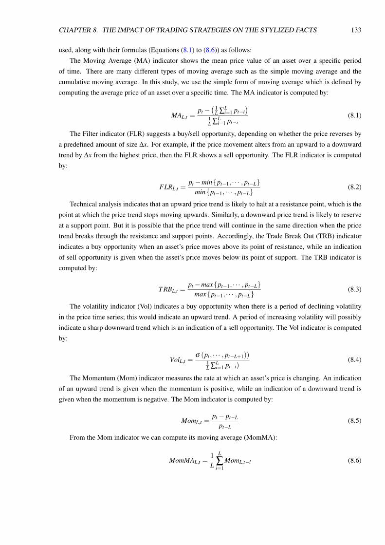
CHAPTER 8. THE IMPACT OF TRADING STRATEGIES ON THE STYLIZED FACTS 133
used, along with their formulas (Equations (8.1) to (8.6)) as follows:
The Moving Average (MA) indicator shows the mean price value of an asset over a specific period
of time. There are many different types of moving average such as the simple moving average and the
cumulative moving average. In this study, we use the simple form of moving average which is defined by
computing the average price of an asset over a specific time. The MA indicator is computed by:
MAL,t =pt −
( 1L ∑
Li=1 pt−i
)1L ∑
Li=1 pt−i
(8.1)
The Filter indicator (FLR) suggests a buy/sell opportunity, depending on whether the price reverses by
a predefined amount of size ∆x. For example, if the price movement alters from an upward to a downward
trend by ∆x from the highest price, then the FLR shows a sell opportunity. The FLR indicator is computed
by:
FLRL,t =pt −min{pt−1, · · · , pt−L}
min{pt−1, · · · , pt−L}(8.2)
Technical analysis indicates that an upward price trend is likely to halt at a resistance point, which is the
point at which the price trend stops moving upwards. Similarly, a downward price trend is likely to reserve
at a support point. But it is possible that the price trend will continue in the same direction when the price
trend breaks through the resistance and support points. Accordingly, the Trade Break Out (TRB) indicator
indicates a buy opportunity when an asset’s price moves above its point of resistance, while an indication
of sell opportunity is given when the asset’s price moves below its point of support. The TRB indicator is
computed by:
T RBL,t =pt −max{pt−1, · · · , pt−L}
max{pt−1, · · · , pt−L}(8.3)
The volatility indicator (Vol) indicates a buy opportunity when there is a period of declining volatility
in the price time series; this would indicate an upward trend. A period of increasing volatility will possibly
indicate a sharp downward trend which is an indication of a sell opportunity. The Vol indicator is computed
by:
VolL,t =σ (pt , · · · , pt−L+1))
1L ∑
Li=1 pt−i)
(8.4)
The Momentum (Mom) indicator measures the rate at which an asset’s price is changing. An indication
of an upward trend is given when the momentum is positive, while an indication of a downward trend is
given when the momentum is negative. The Mom indicator is computed by:
MomL,t =pt − pt−L
pt−L(8.5)
From the Mom indicator we can compute its moving average (MomMA):
MomMAL,t =1L
L
∑i=1
MomL,t−i (8.6)
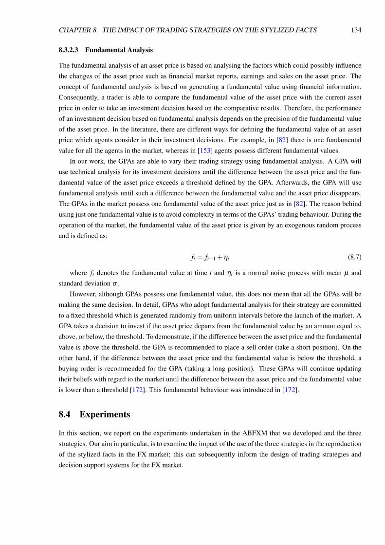
CHAPTER 8. THE IMPACT OF TRADING STRATEGIES ON THE STYLIZED FACTS 134
8.3.2.3 Fundamental Analysis
The fundamental analysis of an asset price is based on analysing the factors which could possibly influence
the changes of the asset price such as financial market reports, earnings and sales on the asset price. The
concept of fundamental analysis is based on generating a fundamental value using financial information.
Consequently, a trader is able to compare the fundamental value of the asset price with the current asset
price in order to take an investment decision based on the comparative results. Therefore, the performance
of an investment decision based on fundamental analysis depends on the precision of the fundamental value
of the asset price. In the literature, there are different ways for defining the fundamental value of an asset
price which agents consider in their investment decisions. For example, in [82] there is one fundamental
value for all the agents in the market, whereas in [153] agents possess different fundamental values.
In our work, the GPAs are able to vary their trading strategy using fundamental analysis. A GPA will
use technical analysis for its investment decisions until the difference between the asset price and the fun-
damental value of the asset price exceeds a threshold defined by the GPA. Afterwards, the GPA will use
fundamental analysis until such a difference between the fundamental value and the asset price disappears.
The GPAs in the market possess one fundamental value of the asset price just as in [82]. The reason behind
using just one fundamental value is to avoid complexity in terms of the GPAs’ trading behaviour. During the
operation of the market, the fundamental value of the asset price is given by an exogenous random process
and is defined as:
ft = ft−1 +ηt (8.7)
where ft denotes the fundamental value at time t and ηt is a normal noise process with mean µ and
standard deviation σ .
However, although GPAs possess one fundamental value, this does not mean that all the GPAs will be
making the same decision. In detail, GPAs who adopt fundamental analysis for their strategy are committed
to a fixed threshold which is generated randomly from uniform intervals before the launch of the market. A
GPA takes a decision to invest if the asset price departs from the fundamental value by an amount equal to,
above, or below, the threshold. To demonstrate, if the difference between the asset price and the fundamental
value is above the threshold, the GPA is recommended to place a sell order (take a short position). On the
other hand, if the difference between the asset price and the fundamental value is below the threshold, a
buying order is recommended for the GPA (taking a long position). These GPAs will continue updating
their beliefs with regard to the market until the difference between the asset price and the fundamental value
is lower than a threshold [172]. This fundamental behaviour was introduced in [172].
8.4 Experiments
In this section, we report on the experiments undertaken in the ABFXM that we developed and the three
strategies. Our aim in particular, is to examine the impact of the use of the three strategies in the reproduction
of the stylized facts in the FX market; this can subsequently inform the design of trading strategies and
decision support systems for the FX market.

CHAPTER 8. THE IMPACT OF TRADING STRATEGIES ON THE STYLIZED FACTS 135
GP parameters ValueMaximum initial tree depth 5Maximum tree depth 9Number of generations 50Population size 50Crossover probability 0.9Mutation probability 0.01Reproduction probability 0.1
Table 8.2: Initial configuration for for the GP parameter values used for the GPAs.
8.4.1 Experimental Setup
The ABFXM operates for a period of one simulated month, where each trading round corresponds to one
simulated second. The main parameters used in the ABFXM can be grouped into three main groups: market,
agent and GP parameters. The initial configuration for the main market and agent parameter values used
in the ABFXM are reported in section 6.9 in chapter 6. Table 8.2 reports the initial configuration for
the GP parameter values for the GPAs. We assess the robustness of the GP parameters by performing a
sensitivity analysis. Furthermore, in order to define the appropriate value for each parameter, we scan each
of the parameter search space individually over a given range of possible values, while keeping the other
parameters at their original values. Such a sensitivity analysis allows us to set an appropriate value for each
parameter of the GP in order for the mechanism to work effectively.
8.4.2 Results
In this section, we report the stylized facts of FX market trading activity established (a) in the real market
data in comparison to those established from the ABFXM populated with: (b) ZI-CV agents; (c) ZI-DCT0
agents; (d) GPAs; a mixture of (e) 50% ZI-CV and 50% ZI-DCT0 agents; (f) 70% ZI-CV and 30% ZI-DCT0
agents; (g) 30% ZI-CV and 70% ZI-DCT0 agents; (h) ZI-DCT0 and GPAs where GPAs <50%; (i) ZI-DCT0
and GPAs where GPAs ≥ 50 %; (j) ZI-CV and GPAs where GPAs <50% and (k) ZI-CV and GPAs where
GPAs ≥ 50% .
The simulation uses historical bid and ask prices for the EUR/USD currency pair over a defined one
month period by feeding these prices into the market and having the agents respond to the price changes.
We use this dataset as the purpose of this work is to explore the impact of various strategies on the trading
activity generated within the ABFXM. The price data are used to anchor the simulation results so that we can
establish whether the transactions data generated by the ABFXM have the same properties as the real market
data. The historical dataset of prices acts as a constant so that multiple simulation runs can be performed
in which different strategies and their impact can be systematically studied without having to worry about
price setting in the market.
The total number of agents in the ABFXM is 104. The only exception is case (d) where the ABFXM
is populated just by GPAs and due to limited computational capacity there are only 8,000 GPAs running.
The stylized facts generated from the ABFXM are averaged over 30 independent simulation runs, each
run being one simulated month, and with different initial seeds provided by random number generators, and
different time horizons over the 2.25 years of the EUR/USD prices data samples. We performed the different
independent simulation runs with the same parameter configuration values but with different seeds and time

CHAPTER 8. THE IMPACT OF TRADING STRATEGIES ON THE STYLIZED FACTS 136
Figure 8.3: The intraday seasonality of the trade numbers from (a) the dataset of EUR/USD transactions,the ABFXM populated with (b) ZI-CV, (c) ZI-DCT0, (d) GPAs, (e) 50% ZI-CV and 50% ZI-DCT0 , (f)70% ZI-CV and 30% ZI-DCT0, (g) 30% ZI-CV and 70% ZI-DCT0, (h) ZI-DCT0 and GPAs (<50%), (i)ZI-DCT0 and GPAs (> 50%), (j) ZI-CV and GPAs (<50%), (K) ZI-CV and GPAs (> 50%).
horizons, to ensure that the results of the simulation are consistent; this allows to establish the robustness
and accuracy of the simulation results.
Seasonality
Figure 8.3 shows the intraday seasonality of the trade numbers from the different data samples as explained
in section 8.4.2 with case (a) being the seasonality exhibited in the real data. From Figure 8.3, the intraday
seasonality of the trade numbers exhibits the double U-shape for two cases when the ABFXM is populated
with (c) just ZI-DCT0 and (h) a mixture of ZI-DCT0 and GPAs (<50%). In contrast, when the ABFXM
is populated with GPAs (> 50%), the U-shape pattern does not emerge. Similarly, all other cases do not
exhibit this intraday seasonality measure. In particular, in the three cases (b, j and k) where the ABFXM is
populated with ZI-CV agents, the intensity of trade numbers increases sharply around 4:00am. Afterwards,
the intensity of trade numbers declines sharply, and then remains very stable throughout the rest of the day,
in contrast to the real market. In all of the three cases where the ABFXM is populated with a mixture of
ZI-CV and ZI-DCT0 agents, the intensity of trade numbers remains stable throughout the day.
Table 8.3 reports the intraday seasonality statistics, the t-statistic values and the Pearson correlation
values where the t-critical value two-tail = 2.07 are presented. According to the paired t-tests with a 95%

CHAPTER 8. THE IMPACT OF TRADING STRATEGIES ON THE STYLIZED FACTS 137
(b) (c) (d) (e)tsv corr tsv corr tsv corr tsv corr
Trade numbers 2.2E-10 - 0.21 -7.1E-10 + 0.98 -3.9E-02 + 0.68 -1.3E-10 +0.52Trade volumes 2.2E-11 - 0.23 4.6E-16 + 0.87 4.7E-02 + 0.50 -7E-10 +0.99Opening positions -2.7E-10 - 0.21 -2.1E-09 + 0.98 -5.3E-02 + 0.66 -1.3E-10 +0.52Closing positions 5.3E-10 - 0.20 2.3E-09 + 0.98 -1.7E-02 + 0.78 1.3E-10 +0.53
(f) (g) (h) (i)Trade numbers -1.3E-10 +0.40 -2.6E-10 +0.32 -3.2E-09 + 0.99 -3.7E-02 + 0.78Trade volumes -1.5E-09 +0.99 -1.5E-09 +0.99 -1.4E-09 + 0.99 5.8E-02 + 0.55Opening positions 5.8E-17 +0.39 -3.9E-10 +0.30 -3.8E-16 + 0.99 -5.2E-02 + 0.70Closing positions 2.5E-10 +0.40 3.8E-10 +0.33 1.5E-09 + 0.99 -1.3E-02 + 0.85
(j) (k)Trade numbers -3.63E-16 -0.23 -2.42E-10 -0.22Trade volumes -1.90E-10 +0.05 -3.75E-11 -0.23Opening positions -1.89E-10 -0.24 -1.21E-10 -0.23Closing positions 2.52E-10 -0.23 3.03E-10 -0.20
Table 8.3: T-statistic (tsv) and Pearson (corr) correlation when the ABFXM is populated with (b) ZI-CV,(c) ZI-DCT0, (d) GPAs, (e) 50% ZI-CV and 50% ZI-DCT0 , (f) 70% ZI-CV and 30% ZI-DCT0, (g) 30%ZI-CV and 70% ZI-DCT0, (h) ZI-DCT0 and GPAs <50%, (i) ZI-DCT0 and GPAs > 50%, (j) ZI-CV andGPAs <50%, (K) ZI-CV and GPAs > 50%.
confidence level linked to the hypothesis (µR− µS = 0), the means of the seasonality statistics in all the
different cases of the simulation results resemble the mean of the seasonality statistics in the real data.
However, the closer correlation results are clearly exhibited by cases (c) and (h) whereas the correlations
in the other cases are not satisfactory. In (b), where the ABFXM is populated just with ZI-CV agents, the
correlations between the seasonality statistics of real data and the simulation data are negative. In (e,f,g),
where the ABFXM is populated with a mixture of ZI-CV and ZI-DCT0 agents, the Pearson correlation
values are low for the trade numbers, while very strong - close to 1 - for the trade volumes. Such results are
of concern as the empirical works reported in the literature indicate that there is a strong correlation between
trade numbers and volumes [63, 117]. In the two cases (j,k), where the ABFXM is populated with a mixture
of ZI-CV agents and GPAs, the Pearson correlation values are negative for the trade numbers, and very low
for the trade volumes where GPAs <50%.
The periodic patterns are correlated with the changes in the behaviour of the worldwide FX market
participants [63]. We believe that the lack of a trading strategy in the ZI-CV agents, may be responsible
for the absence of such periodic patterns. The randomness in the ZI-CV agents’ behaviour also makes it
difficult to interpret the incompatible results between the correlation values for trade numbers and volumes.
Although, the GPA models in our experiments had been calibrated, the use of such strategies do not seem
to yield results close to those of real data. Identifying which of the parameters in the GPAs’ strategy are
responsible for the deviation from the periodic patterns observed in real data is not straightforwad due to
the underlying complexity of the strategy. The experimental results suggest that a random strategy (even
with budget constraints) or a strategy that involves learning are not able to reproduce the stylized facts of
the FX market to a satisfactory extent. The ZI-DCT0 strategy on the other hand which is based on the idea
of identifying perioding patterns and responding to them, seems to achieve results that are close to those of
the real market.

CHAPTER 8. THE IMPACT OF TRADING STRATEGIES ON THE STYLIZED FACTS 138
(a) (b) (c) (d) (e) (f)Trade numbers and volumes + 0.81 + 0.70 + 0.92 + 0.86 + 0.04 + 0.02Buy and sell orders + 0.95 + 1 + 0.99 + 0.85 + 1 + 1Opening and closing positions + 0.98 + 1 + 0.98 + 0.80 + 1 + 1Volatilities and trades + 0.43 - 0.10 + 0.46 + 0.05 - 0.03 + 0.03Volatilities and volumes + 0.28 - 0.06 + 0.31 - 0.01 - 0.09 - 0.03
(g) (h) (i) (j) (k)Trade numbers and volumes + 0.04 + 0.88 + 0.89 + 0.41 + 0.59Buy and sell orders + 1 + 1 + 0.89 + 1 + 1Opening and closing positions + 1 + 0.96 + 0.83 + 1 + 1Volatilities and trades + 0.01 + 0.01 + 0.03 - 0.12 - 0.12Volatilities and volumes - 0.03 - 0.04 - 0.01 + 0.02 - 0.01
Table 8.4: Correlation coefficients computed for the different EUR/USD trading activity from (a) the datasetof EUR/USD transactions, the ABFXM populated with (b) ZI-CV, (c) ZI-DCT0, (d) GPAs, (e) 50% ZI-CVand 50% ZI-DCT0 , (f) 70% ZI-CV and 30% ZI-DCT0, (g) 30% ZI-CV and 70% ZI-DCT0, (h) ZI-DCT0and GPAs (<50%), (i) ZI-DCT0 and GPAs (> 50%), (j) ZI-CV and GPAs (<50%), (K) ZI-CV and GPAs (>50%).
Correlation Behaviour
The correlation between the different trading activities in the FX market data (Table 8.4 (a)), reveal a positive
linear relationship between trade numbers and volumes, numbers of buy and sell executed orders, number
of opening and closing positions, and intraday price volatilities and trade numbers and volumes. From
Table 8.4 (c), we can see that the results when the ABFXM is populated with only ZI-DCT0 agents, case
(c), exhibit very similar correlation behaviour to that of the real data. This means that there are linear
dependencies between the current and past values of the different trading activities in the FX market data.
We believe that the success of the ZI-DCT0 approach in modelling agents is the link between the variations
in price changes and thresholds of different sizes which trigger the agents to trade.
In contrast, in all other cases the correlation is not satisfactory. These results indicate that there is no
dependency between the variations in price changes and the trading activity emerging from the ABFXM
with ZI-CVs or GPAs. The ZI-CV agents trade randomly, subject to budget constraints, and therefore do
not respond to price changes. On the other hand, GPAs use different forms of technical and fundamental
analysis of price changes for their investment decisions, as described in section 8.3.2. Hence, this results in
a variety of decision rules used by the GPAs.
When the ABFXM is populated with a mixture of ZI-CV and ZI-DCT0 agents, cases (e, f, g), this affects
extensively the correlation between the trade numbers and volumes. The statistics show that there is weak
relationship between trade numbers and volumes which is contrary to what has been confirmed using real
market data [63]. Tracking the ZI-CV agents’ trading activity, we found that a low level of cash in their
accounts affects the order size of their trade, which consequently results in a low level of trade volumes in
the market. Low cash in the ZI-CV agents accounts results from their unsuccessful investments during the
simulation run. This explains why there is lack of autocorrelation between ZI-CV agents’ trade numbers
and volumes.

CHAPTER 8. THE IMPACT OF TRADING STRATEGIES ON THE STYLIZED FACTS 139
DC OS DC OSAdj. R2 SE Adj. R2 SE Adj. R2 SE Adj. R2 SE
(a) (c)Trade numbers 0.90 0.37 0.90 0.35 0.91 0.37 0.90 0.31Trade volumes 0.91 0.38 0.90 0.35 0.94 0.35 0.94 0.31Opening positions 0.90 0.35 0.91 0.35 0.92 0.35 0.93 0.31Closing positions 0.90 0.36 0.90 0.35 0.91 0.39 0.90 0.35
(d) (e)Trade numbers 0.79 0.85 0.79 0.70 0.93 0.35 0.91 0.33Trade volumes 0.79 0.86 0.79 0.71 0.95 0.33 0.93 0.35Opening positions 0.78 0.83 0.80 0.72 0.93 0.35 0.89 0.37Closing positions 0.78 0.83 0.80 0.72 0.93 0.35 0.89 0.36
(f) (g)Trade numbers 0.93 0.35 0.77 0.41 0.91 0.37 0.90 0.31Trade volumes 0.97 0.30 0.92 0.35 0.94 0.35 0.94 0.31Opening positions 0.92 0.35 0.77 0.39 0.92 0.35 0.93 0.31Closing positions 0.93 0.35 0.77 0.39 0.91 0.39 0.90 0.35
(h) (i)Trade numbers 0.72 0.61 0.74 0.56 0.80 0.75 0.80 0.72Trade volumes 0.72 0.66 0.72 0.56 0.81 0.76 0.79 0.72Opening positions 0.73 0.57 0.74 0.57 0.80 0.73 0.80 0.74Closing positions 0.78 0.66 0.74 0.54 0.78 0.83 0.80 0.72
(j) (k)Trade numbers 0.91 0.37 - 0.19 1.72 0.84 0.70 - 0.22 1.52Trade volumes 0.94 0.35 0.96 0.35 - 0.19 1.77 - 0.18 1.72Opening positions 0.91 0.37 - 0.19 1.72 0.84 0.70 - 0.22 1.52Closing positions 0.91 0.37 - 0.19 1.72 0.84 0.70 - 0.22 1.52
Table 8.5: The adjusted R2 values of the fits and standard errors (SE), for the scaling laws measured underDC and OS events from (a) the dataset of EUR/USD transactions, the ABFXM populated with (c) ZI-DCT0,(d) GPAs, (e) 50% ZI-CV and 50% ZI-DCT0 , (f) 70% ZI-CV and 30% ZI-DCT0, (g) 30% ZI-CV and 70%ZI-DCT0, (h) ZI-DCT0 and GPAs (<50%), (i) ZI-DCT0 and GPAs (> 50%), (j) ZI-CV and GPAs (<50%),(K) ZI-CV and GPAs (> 50%).
Scaling Laws
The scaling laws as confirmed in the FX market data are plotted in Figure 8.4 (a). Table 8.5 (a) reports
the adjusted R2 values and standard errors of the fits. The existence of the six quantitative relationships
amongst the four scaling laws, holding across EUR/USD trading activity can also be established from the
same figure.
When the ABFXM is populated with just ZI-CVs, case (b), it is not possible to discern the scaling laws
and the dynamics of the trading activity do not match those observed in the real data. As such, the graphs
could not be drawn and hence this case has been omitted from Figure 8.4 and Table 8.5. In detail, and as can
also be observed from Figure 8.3, the intensity of trading activity increases sharply during the few first hours
of the simulation, after which the trading activity declines suddenly and sharply to a much lower level, and
continues to be stable at this very low level during the remaining time of the simulation. We believe that this
is due to the ZI-CV agents’ random stategy and as a consequence their inability to react to price changes in
the market.
The scaling laws and the six quantitative relationships amongst them, are exhibited in the data generated

CHAPTER 8. THE IMPACT OF TRADING STRATEGIES ON THE STYLIZED FACTS 140
Figure 8.4: Scaling laws are plotted where the x-axis shows the price moves thresholds of the EUR/USDobservations and the y-axis shows the average: trade numbers; trade volumes; number of opening positions;and number of closing positions. Scaling laws are defined from (a) the dataset of EUR/USD transactions,the ABFXM populated with (c) ZI-DCT0, (d) GPAs, (e) a mixture of 50% ZI-CV and 50% ZI-DCT0.

CHAPTER 8. THE IMPACT OF TRADING STRATEGIES ON THE STYLIZED FACTS 141
Figure 8.5: Scaling laws are plotted where the x-axis shows the price moves thresholds of the EUR/USDobservations and the y-axis shows the average: trade numbers; trade volumes; number of opening positions;and number of closing positions. Scaling laws are defined from the ABFXM populated with a mixture of (f)70% ZI-CV and 30% ZI-DCT0, (g) 30% ZI-CV and 70% ZI-DCT0, (h) ZI-DCT0 and GPAs (<50%) and (i)ZI-DCT0 and GPAs (> 50%).

CHAPTER 8. THE IMPACT OF TRADING STRATEGIES ON THE STYLIZED FACTS 142
Figure 8.6: Scaling laws are defined from the ABFXM populated with a mixture of (j) ZI-CV and GPAs(<50%), (K) ZI-CV and GPAs (> 50%).
from the ABFXM populated with just ZI-DCT0 agents, Figure 8.4 (c). Table 8.5 (c) reports the adjusted R2
values and standard errors of the fits. The significance of the fit of the line which is an indication of linear
dependency between the different sizes of the price movements and the observed market trading activity
measured at these different sizes of price movements, is obvious from the adjusted R2 values. The standard
errors of the fits are roughly equivalent to the estimated errors for scaling laws in the empirical data reported
in Table 8.5 (a). We therefore conclude that a key element in modelling the agents’ strategies is the linking
of variations in price changes to thresholds of different sizes in order to trigger trading behaviour on the part
of the agents.
In the three cases (e, f, g), where the ABFXM is populated with a mixture of ZI-CV and ZI-DCT0 agents,
surprisingly the simulation results exhibit the scaling laws according to the adjusted R2 values, Table 8.5
(e, f, g). However, the six quantitative relationships amongst the scaling laws are not exhibited, as shown
from Figure 8.4 (e) and 8.5 (f, g). Additionally, the trade numbers are much higher than in the real FX
market data, as can be seeing from Figure 8.4 (a). Such results are questionable, in that unrealistically high
trade numbers occur during DC and OS events. One possible reason is that the ZI-CVs do not react to price
changes in the market, and consequently do not consider a DC event as a pattern set up for the price trend
movement. Such a pattern influences agents’ decisions, assuming that the current price trend will continue
in the same direction or move in the opposite direction. Therefore, this might explain why the DC and OS
events contain roughly the same number of trades in the ABFXM populated with ZI-CVs. This is in contrast
to the real FX market data wherein an OS event contains twice as many trades as a DC event.
The scaling laws and the quantitative relationships amongst them are not exhibited in the data produced
from the ABFXM populated with just GPAs or a mixture of ZI-DCT0 and GPAs, Figure 8.4 (d) and 8.5 (h,

CHAPTER 8. THE IMPACT OF TRADING STRATEGIES ON THE STYLIZED FACTS 143
(b) (c) (d) (e)ZI-CV ZI-DCT0 GPAs ZI-CV ZI-DCT0
Min - 100 % -100 % - 99.50% - 100 % - 100 %Max - 99.90 % 3693.68 % 1169.86% - 99.90 % 921.84%Average - 99.99 % 13.13 % - 27.49% - 99.99 % 921.84%Winning 0 44.90% 23.10% 0 47.08%Losing 100 % 55.10% 76.90% 100 % 52.92%
(f) (g)ZI-CV ZI-DCT0 ZI-CV ZI-DCT0
Min - 100 % - 100 % - 100 % -100%Max - 99.90 % 22.47% - 99.90 % 711.02%Average - 99.99 % 22.47% - 99.99 % -6.77%Winning 0 45.40% 0 42.69%Losing 100 % 54.60% 100 % 57.31%
(h) (i)GPAs ZI-DCT0 GPAs ZI-DCT0
Min - 99.25% - 99.97% - 99.79% - 100%Max 38.42% 419.75% 1169.86% 780.16%Average - 29.63% - 4.21% - 27.49% 3.30%Winning 31.58% 34.08% 23.10% 40.73%Losing 68.42% 65.92% 76.90% 59.27%
(j) (K)ZI-CV GPAs ZI-CV GPAs
Min - 100 % -99.08% - 100 % -99.47%Max - 100 % 330.27% - 100 % 258.66%Average - 100 % -8.41% - 100 % -36.92%Winning 0 30% 0 14.25%Losing 100 % 70% 100 % 85.75%
Table 8.6: Descriptive statistics of the agents’ ROI from the ABFXM populated with (b) ZI-CV, (c) ZI-DCT0, (d) GPAs, (e) 50% ZI-CV and 50% ZI-DCT0 , (f) 70% ZI-CV and 30% ZI-DCT0, (g) 30% ZI-CVand 70% ZI-DCT0, (h) ZI-DCT0 and GPAs (<50%), (i) ZI-DCT0 and GPAs (> 50%), (j) ZI-CV and GPAs(<50%), (K) ZI-CV and GPAs (> 50%).
i). From Table 8.5 (d, h, i), the adjusted R2 values are not very close to 1, which implies non-significant
fit. The scaling laws are exhibited under DC events from the ABFXM populated with a mixture of ZI-CV
and GPAs where GPAs <50% (Figure 8.6 - j). The adjusted R2 values in Table 8.5 - j shows the significant
of the fit. However, the scaling laws of trade numbers are not exhibited under OS events from the ABFXM
populated with a mixture of ZI-CV and GPAs where GPAs <50%. The adjusted R2 values in Table 8.5 - k are
negative. When the ABFXM is populated with a mixture of ZI-CV and GPAs where GPAs > 50% (Figure
Figure 8.6 - k), the scaling laws are not exhibited. According to the results, the ensuing GPAs’ behaviour in
the ABFXM does not reproduce the scaling laws, thus supporting other studies which emphasize that some
properties in the financial markets may not indeed be the result of interactions between agents who possess
sophisticated learning and adaptation mechanisms [5, 64, 225].
Return on Investment (ROI)
ROI is a performance measure which is defined as the total return with regard to an agent’s investment
over a defined period, divided by the cost of the investment. The ROI is expressed as a percentage and can
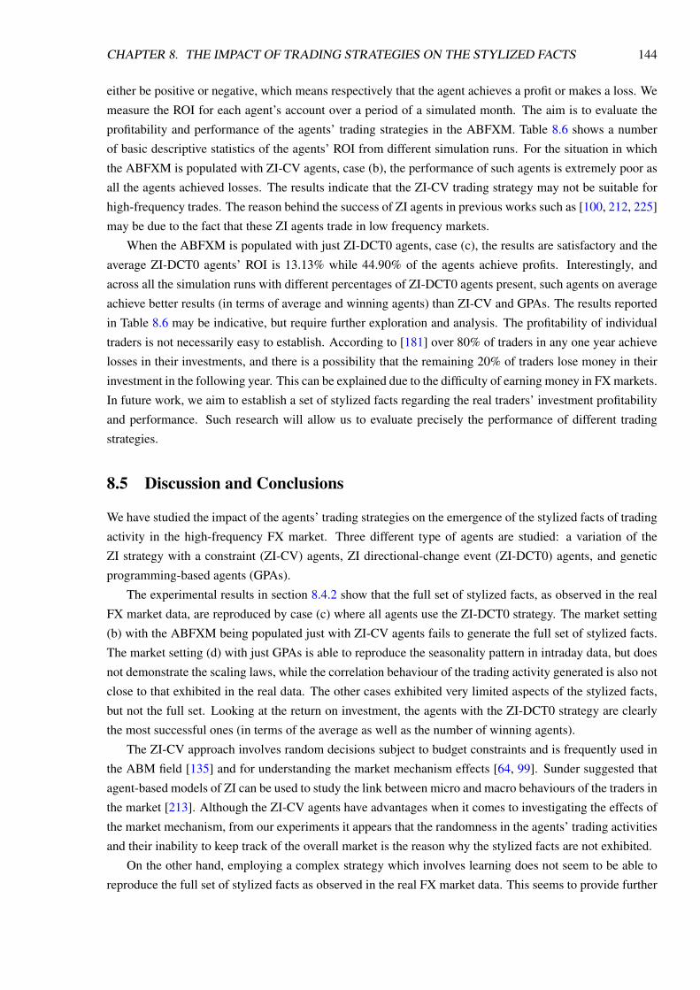
CHAPTER 8. THE IMPACT OF TRADING STRATEGIES ON THE STYLIZED FACTS 144
either be positive or negative, which means respectively that the agent achieves a profit or makes a loss. We
measure the ROI for each agent’s account over a period of a simulated month. The aim is to evaluate the
profitability and performance of the agents’ trading strategies in the ABFXM. Table 8.6 shows a number
of basic descriptive statistics of the agents’ ROI from different simulation runs. For the situation in which
the ABFXM is populated with ZI-CV agents, case (b), the performance of such agents is extremely poor as
all the agents achieved losses. The results indicate that the ZI-CV trading strategy may not be suitable for
high-frequency trades. The reason behind the success of ZI agents in previous works such as [100, 212, 225]
may be due to the fact that these ZI agents trade in low frequency markets.
When the ABFXM is populated with just ZI-DCT0 agents, case (c), the results are satisfactory and the
average ZI-DCT0 agents’ ROI is 13.13% while 44.90% of the agents achieve profits. Interestingly, and
across all the simulation runs with different percentages of ZI-DCT0 agents present, such agents on average
achieve better results (in terms of average and winning agents) than ZI-CV and GPAs. The results reported
in Table 8.6 may be indicative, but require further exploration and analysis. The profitability of individual
traders is not necessarily easy to establish. According to [181] over 80% of traders in any one year achieve
losses in their investments, and there is a possibility that the remaining 20% of traders lose money in their
investment in the following year. This can be explained due to the difficulty of earning money in FX markets.
In future work, we aim to establish a set of stylized facts regarding the real traders’ investment profitability
and performance. Such research will allow us to evaluate precisely the performance of different trading
strategies.
8.5 Discussion and Conclusions
We have studied the impact of the agents’ trading strategies on the emergence of the stylized facts of trading
activity in the high-frequency FX market. Three different type of agents are studied: a variation of the
ZI strategy with a constraint (ZI-CV) agents, ZI directional-change event (ZI-DCT0) agents, and genetic
programming-based agents (GPAs).
The experimental results in section 8.4.2 show that the full set of stylized facts, as observed in the real
FX market data, are reproduced by case (c) where all agents use the ZI-DCT0 strategy. The market setting
(b) with the ABFXM being populated just with ZI-CV agents fails to generate the full set of stylized facts.
The market setting (d) with just GPAs is able to reproduce the seasonality pattern in intraday data, but does
not demonstrate the scaling laws, while the correlation behaviour of the trading activity generated is also not
close to that exhibited in the real data. The other cases exhibited very limited aspects of the stylized facts,
but not the full set. Looking at the return on investment, the agents with the ZI-DCT0 strategy are clearly
the most successful ones (in terms of the average as well as the number of winning agents).
The ZI-CV approach involves random decisions subject to budget constraints and is frequently used in
the ABM field [135] and for understanding the market mechanism effects [64, 99]. Sunder suggested that
agent-based models of ZI can be used to study the link between micro and macro behaviours of the traders in
the market [213]. Although the ZI-CV agents have advantages when it comes to investigating the effects of
the market mechanism, from our experiments it appears that the randomness in the agents’ trading activities
and their inability to keep track of the overall market is the reason why the stylized facts are not exhibited.
On the other hand, employing a complex strategy which involves learning does not seem to be able to
reproduce the full set of stylized facts as observed in the real FX market data. This seems to provide further

CHAPTER 8. THE IMPACT OF TRADING STRATEGIES ON THE STYLIZED FACTS 145
support to studies such as [64, 99, 100, 189, 225] that have argued that complex strategies and in particular
strategies that involve learning may not be necessary nor sufficient for the emergence of phenomena such as
stylized facts emerging in markets. In our work, we have attempted to calibrate the parameters of the GPAs,
but the wide variance in the decision rules that GPAs use does not allow us to pinpoint a single element
of the GPAs’ trading strategy mechanism as being one of the factors accountable for the non-emergence
of the stylized facts. The complexity in the GPAs’ trading strategy makes it difficult to draw out general
conclusions regarding the results or inputs of the GPAs’ trading activity in the market. Unlike the ZI-DCT0
strategy, the GPAs’ forecasting mechanism for detecting patterns in price time series using various technical
indicators as the main tool, is more complex. The character and structure of these detected patterns can
be of different magnitude and can use different time scales to unfold. For instance, the Santa Fe Artificial
Stock Market (SF ASM) is populated by heterogeneous agents whose trading strategies involve learning,
evolutionary processes and a classifier system. The SF ASM is able to reproduce some of the stylized facts
observed in stock markets. However, the interaction of these agents makes explaining the stylized facts of
the stock market behaviour a very difficult task [135].
The ZI-DCT0 strategy avoids the complexity of GPAs and also the randomness of the ZI-CV strategy.
ZI-DCT0 agents respond to periodic patterns in the price time series of a fixed size. This relatively simple
strategy appears to be effective in the HF FX market and the experiments suggest that this kind of behaviour
is able to reproduce the stylized facts observed in the real market. The scaling law relations in the HF FX
data also seem to suggest that these highly depend on the agents’ responses to different price fluctuations.
Our results provide evidence that introducing a threshold for the agents to trade when the price fluctuations
exceed the threshold represents a key element in for an agent’s trading strategy in the HF FX. The authors in
[64, 69, 99, 110, 143, 189, 193] stress the importance of simplicity in building agent-based models in order
to make possible the understanding of market behaviour and the forces driving the market. We believe that
the ZI-DCT0 strategy allows us to gain a good insight into market behaviour dynamics without having to
make various assumptions about the strategic behaviour of the agents.

Chapter 9
Conclusions
This chapter provides a summary of the work presented in this thesis (section 9.1), identifies the thesis
contributions to the area of ABMs (section 9.2), and describes some potential avenues for future research
by which this work can be extended (section 9.3).
9.1 Summary
One of the principle goals of agent-based simulations is to study and understand complex real-life phenom-
ena, where the use of analytical models is not applicable. ABMs have emerged as a means of studying the
behaviour of individual agents within a market setting, the interaction effects, emergent macro properties,
collective behaviour, and the impact of market rules or policies, among others.
The aim of this thesis is to contribute to the research area of ABMs by identifying the essential elements
under which the stylized facts of the trading activity in the high-frequency FX markets are exhibited in an
ABM. This consequently implies that the areas of FX markets and ABMs have to be studied, described and
their relevant literature reviewed. In chapter 2, we start by describing the FX market structure and associated
studies on FX market behaviour. As FX markets generate masses of data we discuss high frequency data
and the challenges associated with their processing and analysis. We subsequently review the state of the
art in the ABM area including key design issues in the development of ABMs. The chapter also includes a
brief overview of artificial intelligence techniques, and in particular, evolutionary computation ones that are
commonly used in financial forecasting.
Before developing an ABFXM, the trading activity in the high-frequency FX markets has to be observed,
analyzed and properly understood. Therefore, the first research step focuses on defining a proper effective
approach for analyzing and studying the financial markets’ behaviour. This is the subject of chapter 3.
Surveying the literature we found an effective approach which is the directional-change event introduced
by Guillaume et al. in [104], where events of different magnitudes are the time-scale of the time series.
Financial markets are highly active at some times, but calm at others. Therefore using fixed time scales runs
the risk of missing important activities. An alternative approach is to focus on directional-change events
that capture periodic activities in the market. In chapter 3, we showed the potential significance of the
directional-change event approach for studying and analyzing financial markets. Our study confirmed that
the length of the price curve coastline, as defined by directional-change events, turns out to be a long one.
We showed by means of experimental results that automated trading algorithms could potentially be derived
by means of directional-change events.
146

CHAPTER 9. CONCLUSIONS 147
Having the essential tools for observing, analyzing and studying the trading activity in the FX market,
next comes the fundamental step of our study which is establishing stylized facts of the trading activity in
the high-frequency FX market. To establish stylized facts of the trading activity, we need to explore high-
frequency data of individual traders’ historical transactions in the FX market. Fortunately, our study has
acquired a unique high-frequency dataset of individual traders’ historical transactions on the OANDA FX
trading platform over 2.25 years. Prior to analyzing and studying the dataset, we have conducted a filtering
procedure to remove misleading and spurious data from the dataset, in chapter 4. The filtering process is an
essential step prior to the analysis of a high-frequency dataset, in that failure to recognize misleading and
spurious data will affect the validity of the results derived from the analysis. Validating the adopted filtering
procedure, we confirmed a clean transaction dataset. We have shown the behaviour and effects of both the
original and filtered datasets in the exhibition of the intraday seasonality of the trade numbers in FX market
which confirms the impact of the filtering process on the validity of the analysis of high-frequency datasets.
In chapter 5, we analysed and studied the dataset. Our work confirms established stylized facts of
seasonality and correlation behaviour in the literature [63, 117] but also goes beyond those as we have
discovered four new scaling laws and established six quantitative relationships amongst them, holding across
EUR/USD and EUR/CHF transactions. Given a fixed threshold (∆x), the observed four new scaling laws
state that the average (a) trade numbers, (b) trade volumes, numbers of (c) opening and (d) closing positions
observed during an event of size ∆x is scale-invariant to the size of this threshold (∆x). The established
stylized facts of the trading activity in high-frequency FX markets can offer insights into the market workings
and traders’ behaviour but also serve as a benchmark for validating agent-based models of FX markets.
In chapter 6, we have constructed an ABFXM which simulates the intraday trading activity at the level
of a FX market-maker market. The ABFXM is able to reproduce the stylized facts of the trading activity
as exhibited in the real FX market. This is confirmed by the statistical analysis. Our study uses the his-
torical dataset provided by OANDA to anchor the results of the simulation. The ABFXM has a number of
distinguishing features including: modelling heterogeneity in different forms; asynchronous trading-time
windows, the generation of limit orders and an approach for determining an agent’s order size. The agents
have been modelled as simple zero-intelligence directional-change event trading (ZI-DCT0) agents. The
ZI-DCT0 agents commit themselves to a fixed threshold to detect periodic fixed patterns in the price time
series. The individual agents are characterised by different levels of wealth, different profit objectives and
risk appetites and initial activation conditions.
Chapter 7 presents a systematic experimental examination by varying a number of elements of the
ABFXM. Such experimentation aimed to evaluate the effects of the different elements on reproducing the
stylized facts observed in the empirical data. This allowed us to identify the set of essential elements that
should be present in an ABM in order to reproduce the stylized facts of the trading activity in the high-
frequency FX market to a satisfactory extent. Our study suggests that among the key elements that affect
the emergence of stylized facts are the number of agents in the market and heterogeneity in the agents’
strategies which in our model takes a number of forms: varying profit objectives, risk appetites and wealth
distribution. The generation of limit orders also seem to play an important role as this provides another
dimension to the agent’s trading strategy coupled with orders of varying size. The mixture of contrarian and
trend-following ZI-DCT0 agents in the market also seem to have an impact in the emergence of stylized
facts. We have been able to study extensively the effect of each of the constituent elements of the market
on the stylized facts through anchoring the simulation results by using a historical transactions dataset. The

CHAPTER 9. CONCLUSIONS 148
use of this dataset enables to run multiple simulation runs and draw comparisons and conclusions for each
market setting against the real data but also by comparing different market settings.
Chapter 8 can be considered as an extension of chapter 7. In this chapter we discussed the design issue
of the type and structure of the agents’ trading strategies in an ABFXM. We explored the effects of three al-
ternative approaches to the design of the agents’ trading strategies: a variation of the zero-intelligence with
a constraint (ZI-CV) strategy; the zero-intelligence directional-change event (ZI-DCT0) strategy; and the
genetic programming-based (GP) strategy. A series of experiments were conducted on the ABFXM which
populated with these three agent-based models and the results were compared against a high-frequency
dataset from the FX market. Understanding the market workings through stylized facts is fundamental for
developing more effective decision support systems. The results of this study suggest that the ZI-DCT0
strategy is particularly suitable for approximating the stylized facts of the FX market activity and in com-
parison with the other strategies also has achieved better results in terms of Return on Investment (ROI).
Hence, we could suppose that the observed properties of the trading activity in the FX market could be the
result of introducing a threshold which triggers the agents to respond to fixed periodic patterns in the price
time series. As such, our study also suggests that being able to recognise patterns in the time series such
as DC and OS events may be key to providing effective decision support in the FX markets. The simple
learning mechanism employed by the ZI-DCT0 is clearly more effective than the GP strategy which uses
a series of technical indicators and fundamental analysis. Although, we cannot draw more generic conclu-
sions about the use of other learning strategies in the FX market, our results provide evidence that a complex
learning strategy may not be necessary.
9.2 Contributions
The presented work in this thesis is contributing to the area of ABMs. In this thesis, we have made the
following major contributions:
• We have used an extensive high-frequency FX transactions dataset for the stylized facts study. In addi-
tion, the ABFXM uses a high-frequency historical prices dataset which enables more comprehensive
experiments to be run.
• We have established a number of stylized facts that characterise the trading activity in the high-
frequency FX market which can serve as a benchmark for validating agent-based FX markets. As
part of the stylized facts analysis we uncovered four new scaling laws and six quantitative relation-
ships among them holding across the FX market transactions data.
• We have constructed an ABFXM able to approximate the stylized facts of the trading activity as ex-
hibited in the corresponding real FX markets to a satisfactory extent as demonstrated by the statistical
analysis. Our aim was to construct an ABFXM that on the one hand would be able to exhibit the
discovered stylized facts, but on the other, would not be overly complex so that it could prevent us
from clearly studying and analyzing its behaviour. To the best of our knowledge, this is the first work
modelling the trading activity in the high-frequency FX market.
• We have identified a set of essential elements that characterise the FX market and affect the emergence
of the stylized facts of the trading activity in this market. To the best of our knowledge, the thesis

CHAPTER 9. CONCLUSIONS 149
presents the first study where a search for the essential elements under which the stylized facts of the
trading activity in the high-frequency FX market emerge as a consequence in an ABM.
• We have examined three different approaches for the design of the agents’ trading strategies in an
ABFXM. The aim is to show the effect of the agents’ trading strategies on approximating the stylized
facts and understanding the trading in the FX market. To our knowledge, this is the first study which
experiments with different strategies on the FX market, studies and analyses the ensuing behaviour.
The major contributions we have made in this thesis are supported by the following contributions:
• We have measured the length of the price-curve coastline, which represents the profit potential, under
physical time (fixed time intervals) and intrinsic time (directional-change events). The measurement
shows a long coastline of price changes defined by intrinsic time. We have also measured the total
error of the length of the price curve coastline under both physical and intrinsic time. The results
confirmed that studying the price time series using intrinsic time gives a more advanced description
of price changes than does using physical time with fixed time intervals.
• We performed a customized filtering procedure to eliminate misleading and spurious data from the
high-frequency dataset of individual traders’ historical transactions on the OANDA FX trading plat-
form.
• We have modelled a simple zero-intelligence directional-change event trading (ZI-DCT0) agents. This
is different from other works in the literature [5–7, 21, 42, 46, 48, 49, 52, 56, 64, 83, 95, 100, 114,
128, 138, 146, 149, 150, 153, 158, 159, 170, 172, 215, 232, 238] as the ZI-DCT0 agents avoids the
complexity of intelligent strategic behaviour and also the vagueness of zero-intelligence strategy in
which agents trade randomly subject to budget constraint. We show that the stylized facts of real
markets can be reproduced by ZI-DCT0 agents, subject to budget constraints. We believe that this is
the first such work that is able to demonstrate this.
• The modelling of heterogeneity in different forms. Heterogeneity is inherent in real markets, so
in creating ABMs this is an important characteristic that needs to be modelled. Heterogeneity in
our ABM is modelled in the agents’ initial wealth, leverage ratio used by the agents, their trading
strategies, their profit objectives, their risk appetites, and their trading windows which represent ge-
ographical distribution. Whereas there are other works that have modelled heterogeneity such as
[5–7, 21, 46, 49, 52, 64, 83, 95, 114, 138, 146, 149, 150, 153, 158, 159, 170, 172, 232, 238], these do
so in a limited way or through a small number of elements. No other work in the literature has used
as many and as varying elements to model heterogeneity as we have.
• We have modelled asynchronous trading in our ABFXM as present in real markets. To this end,
we have considered four important factors: the agents’ activation time in the market, the notion of
market business hours, holidays and the introduction of a threshold to trigger the agents’ activities.
Again this is in contrast with what has been done in the literature to date where a number of ABMs
entail continuous-time trading which means that at each time of the market each agent updates their
beliefs and as a result places an order or holds [120, 172]. Employing continuous-time trading in
an ABM results in a rise in the computational cost since at every time in the market each agent
has to perform some trading computation. Hence, the computational cost has to be considered in

CHAPTER 9. CONCLUSIONS 150
the design of an ABM. An alternative approach is proposed by the Genoa artificial stock market
[188] where the determination of the agents who will be active in the next time step in the market is
drawn randomly. Nevertheless, such randomisation is not sufficient considering that it might introduce
ambiguity regarding the arrival time of the order.
• The construction of a new approach for determining an agent’s order size which is based on the agent’s
available margin and drawing randomly within a defined range. The advantage of this new approach is
that it provides a further source of heterogeneity in the agents’ trading activities and hence the market.
This is unlike other works in the literature where the agent’s order size is (a) proportional to its wealth
[120]; (b) a fraction of its cash, based on a constant trading proportion parameter [137, 171, 172, 188].
These two approaches lack heterogeneity in terms of the amount of an agent’s investments during the
market run. In addition, the first approach results in inducing a high trading risk seeing that an agent
invests the full cash it holds in a single order. Similarly, in the second approach, a high value of
the trading proportion parameter also results in high trading risk for the agent. High trading risk
sequentially causes cascading margin calls in the market, which persuade a price drop in the market
and accordingly affect the agent’s performance.
• We have studied the impact of changing the different elements of the ABFXM on the market behaviour
and their effect on reproducing the stylized facts observed in the empirical data. Such a study is the
core step towards achieving the thesis aim which is identifying a set of essential elements under which
the stylized facts of the trading activity in the FX market are exhibited in an ABM.
9.3 Future Work
This thesis offers the first agent-based model of the trading activity in the high-frequency FX market. Despite
the fact that the thesis has achieved its intended aim and objectives, further work can extend this study and
provide further insights into the workings of the high-frequency FX market:
• Although we have established a set of stylized facts from the high-frequency transactions dataset that
was made available to this study by OANDA, the dataset is very rich in information and it would be
worth extending its study. In particular, further analysis could establish more stylized facts regarding
the FX market trading activity and traders’ portfolios. Identifying more stylized facts facilitates and
improves our understanding of FX market behaviour and, most importantly, allows us to identify the
forces that drive the traders’ behaviour in such markets. Having more stylized facts would also enable
us to validate the ABFXM further but also conduct further experiments to investigate their origins.
• As we have established that the developed ABFXM is able to approximate the FX market stylized
facts when fed with real historical prices data, as part of further work, this feed can be removed so
that the market-maker can generate artificial prices. Market-makers in the FX market generate prices
by observing the demand and supply in the market, historical information, information about current
political and economic events and other factors. Hence, studying price formation through the market-
maker component of the ABFXM could further our understanding of the FX market workings and
would also enable the study of the characteristics of the price time series generated. In addition, more
than one market maker could be modelled to enable the study of such competition in the market and

CHAPTER 9. CONCLUSIONS 151
the impact on the price time series. There are some interesting studies already being done in the
subject of modelling the competition between market-makers [35, 133, 134, 177].
• In the present work and to facilitate the analysis, the ABFXM only includes one traded currency pair.
Further work can explore including more than one traded assets in the market and as a result more
complex strategies for the trading agents.
• Although the ABFXM allows margin trading (use of leverage), we have not examined and studied
the impact of leverage on the emergence of the stylized facts either on the traders’ performance or
the results of cascading margin calls. Such a study would require a series of controlled experiments
where the agents’ wealth and the desired order size must be considered.
There are several noteworthy avenues for future research that the work presented in this thesis can contribute
to, including the following:
• Establish a foundation for modelling traders’ behaviour from the microscopic analysis of the individ-
ual traders’ transactions in the FX market. The statistical results from the microscopic analysis could
provide a foundation of useful tools for predicting price movements in the market in order to identify
investment arbitrage opportunities.
• Define the individual trader’s adopted trading strategies through observing and analyzing the high-
frequency dataset of OANDA individual traders’ historical transactions. The aim is to assess the
trading strategies’ performance by identifying and evaluating the strategies adopted. Accordingly,
one could assess and classify the trading strategies that would lead to success or failure.
• Study the interaction between different types of trading strategies, such as trading strategy based on
directional-change event approach, Zero-Intelligence Plus (ZIP) [55] and Adaptive Aggressiveness
(AA) [228]. The aim is evaluating different adopted strategies by assessing the traders’ investment
performance in the market. This in turn could help us answer a number of questions which have arisen
such as: which adopted trading strategy leads to success or failure under different circumstances?
Which trading strategies are most efficient? Going even further, more work could be done in observing
the results of the interactions between different trading strategies. Such observations, on one hand,
can be used as feedback to change the models of interaction, and on the other hand can provide
exploration of some traders’ behavioural phenomena such as herding behaviour. ABMs enable us to
study and test scientifically different trading strategies.
• Compare different market mechanisms for the high-frequency FX market. Such a comparison study
helps in answering a variety of questions such as: what are the implications of the market mecha-
nism in the price formation? Does the setting of the market mechanism attract more trading activity;
increase price volatility; increase the likelihood of market collapse? Furthermore, such a study can
potentially help to design and evaluate new market mechanisms. Obviously, it would be unimaginable
to launch new market rules before analyzing and studying their impact thoroughly.
• Examine the effects of the agents’ type and structure in the appearance of the stylized facts of price
returns and order-flow in an ABM. The results will be significant in providing comprehensive details
of the effects of the agents’ strategic behaviour on the emergence of the market stylized facts in an
ABM.

CHAPTER 9. CONCLUSIONS 152
• In response to the financial crises, the constructed ABFXM can be used as an experimental laboratory
for exploring and identify conditions as a result of which collapses occur in the market. Simulations
have the potential to answer essential questions such as: under what conditions does price collapse
occur? Can we identify early signs of market crisis? How can the market rules be improved to avoid
excessive price collapses? A mechanism for forecasting financial crises must be developed, along
with a means by which we can analyse patterns with regard to what has happened prior to the crisis.
An early warning system for the financial market can be a solution to providing early indications of a
financial crisis to prevent enormous losses toward improvement of the market efficiency.
• The directional-change event approach opens doors to several avenues of future research into financial
markets. One promising research direction is to use the directional-change event approach in study-
ing volatility and measuring trading risk in the market. Going further, the directional-change event
approach can be of significant use in building forecasting models regarding the behaviour of prices in
the market.
We aim to explore some of these avenues in our future research.

Bibliography
[1] Aguirre, M., and R. Said (1999), Feedback trading in exchange-rate markets: evidence from within
and across economic blocks, Journal of Economics and Finance, 23, 1–14. 1, 15
[2] Alexandrova-Kabadjova, B., E. Tsang, and A. Krause (2011), Market structure and information in
payment card markets, International Journal of Automation and Computing, 8, 364–370. 2
[3] Alfarano, S., and T. Lux (2006), A minimal noise trader model with realistic time series properties,
Economics Working Papers 11, Christian-Albrechts-University of Kiel, Department of Economics.
21
[4] Alfarano, S., T. Lux, and F. Wagner (2005), Estimation of agent-based models: the case of an asym-
metric herding model, Computational Economics, 26(1), 19–49. 21
[5] Alfi, V., M. Cristelli, L. Pietronero, and A. Zaccaria (2009), Minimal agent based model for financial
markets I: origin and self-organization of stylized fatcs, The European Physical Journal B, 67(3),
385–397. 2, 5, 11, 17, 18, 22, 23, 71, 76, 77, 92, 116, 124, 128, 143, 149
[6] Alfi, V., M. Cristelli, L. Pietronero, and A. Zaccaria (2009), Minimal agent based model for financial
markets II: statistical properties of the linear and multiplicative dynamics, The European Physical
Journal B, 67(3), 399–417.
[7] Alfi, V., M. Cristelli, L. Pietronero, and A. Zaccaria (2009), Mechanisms of self-organization and
finite size effects in a minimal agent based model, J. Stat. Mech, P03016. 2, 5, 17, 78, 92, 116, 124,
128, 149
[8] Allais, M. (1974), The psychological rate of interest, Journal of Money Credit and Banking, 3, 285–
331. 29
[9] Allen, F., and R. Karjalainen (1999), Using genetic algorithms to find technical trading rules, Journal
of Financial Economics, 51, 245–271. 24
[10] Almeida, A., C. Goodhart, and R. Payne (1998), The effects of macroeconomic news on high fre-
quency exchange rate behavior, Journal of Financial and Quantitative Analysis, 33, 383–408. 1,
15
[11] Amilon, H. (2008), Estimation of an adaptive stock market model with heterogeneous agents, Journal
of Empirical Finance, 15(2), 342–362. 21
153

BIBLIOGRAPHY 154
[12] Ammermann, P., and D. Patterson (2003), The cross-sectional and cross-temporal universality of
nonlinear serial dependencies: evidence from world stock indices and the taiwan stock exchange,
Pacific-Basin Finance Journal, 11(2), 175–195. 12
[13] Andersen, T. (2000), Some reflections on analysis of high-frequency data, Journal of Business and
Economic Statistics, 18, 146–153. 26
[14] Andersen, T., and T. Bollerslev (2003), Micro effects of macro announcements: real-time price dis-
covery in foreign exchange, American Economic Review, 93, 38–62. 1, 15
[15] Arifovic, J. (1994), Genetic algorithm learning and the cobweb model, Journal of Economic Dynam-
ics & Control, 18, 3–28. 2, 20, 21
[16] Arifovic, J. (1996), The behavior of the exchange rate in the genetic algorithm and experimental
economics, Journal of Political Economy, 104(3), 510–541. 20, 21
[17] Arifovic, J. (2001), Evolutionary dynamics of currency substitution, Journal of Economic Dynamics
& Control, 25, 395–417. 2
[18] Armer, J. (1998), Market force, ecology, and evolution, Industrial and Corporate Change, 11, 895–
953. 3, 27
[19] Arrow, K. (2004), The changing face of economics, in Conversations with cutting edge economists,
edited by D. Colander, R. Holt, and J. Rosser, University of Michigan Press, Ann Arbor. 107
[20] Arthur, W. (1991), Designing economic agents that act like human agents: a behavioral approach to
bounded rationality, American Economic Review, 81, 353–359. 1
[21] Arthur, W. B., J. H. Holland, B. LeBaron, R. Palmer, and P. Tayler (1997), Asset pricing under
endogenous expectations in an artificial stock market, in The economy as an evolving, complex system
II, edited by W. Arthur, D. Lane, and S. Durlauf, pp. 15–44, Addison Wesley, Redwood City, CA. 1,
2, 3, 5, 16, 20, 21, 22, 23, 25, 27, 92, 127, 149
[22] Atkinson, A., and A. Harrison (1978), Distribution of Total Wealth in Britain, Cambridge University
Press, Cambridge. 72, 105
[23] Austin, M., G. Bates, M. Dempster, V. Leemans, and S. Williams (2004), Adaptive systems for
foreign exchange trading, Quantitative Finance, 4(4), 37–45. 16, 24, 127
[24] Azoff, E. (1994), Neural Network Time Series Forecasting of Financial Markets, John Wiley & Sons,
Inc., New York, NY, USA. 24
[25] Bachlier, L. (1964), Theory of speculation in the random character of stock market prices, MIT Press,
Cambridge. 1
[26] Bak, P., M. Paczuski, and M. Shubik (1997), Price variations in a stock market with many agents,
Physica A, 246, 430–453. 20, 21
[27] Ballocchi, G., M. Dacorogna, C. Hopman, U. Müller, and R. Olsen (1999), The intraday multivariate
structure of the euro futures markets, Journal of Empirical Finance, 6, 479 – 513. 14

BIBLIOGRAPHY 155
[28] Barber, B., and T. Odean (2000), Trading is hazardous to your wealth: The common stock investment
performance of individual investors, Journal of Finance, 55, 773 – 806. 1, 15
[29] Barberis, N., and R. Thaler (2003), A survey of behavioral finance, Tech. Rep. 9222, NBER. 1, 14
[30] Batchelor, R., and G. Albanis (2001), Predicting high performance stocks using dimensionality re-
duction techniques based on neural networks, in Developments in Forecast Combination and Portfolio
Choice, edited by C. Dunis and A. Timmerman, pp. 117–134, Kluwer Academic Publishers. 24
[31] Bauer, R. (1994), Genetic Algorithms and Investment Strategies, John Wiley & Sons, New York. 24
[32] Becker, G. (1962), Irrational behaviour and economic theory, Journal of Political Economy, 70, 1–13.
20, 127
[33] Beja, A. (1977), The limits of price information in market processes, Tech. Rep. 61, Research Program
in Finance, University of California, Berkeley. 1, 10, 11
[34] Berger, D., A. Chaboud, S. Chernenko, E. Howorka, and J. Wright (2006), Order flow and exchange
rate dynamics in electronic brokerage system data, Tech. Rep. 830, Board of Governors of the Federal
Reserve System, International Finance. 1, 2, 15
[35] Biais, B., D. Martimort, and J. Rochet (2000), Competing mechanisms in a common value environ-
ment, Econometrica, Econometric Society, 68(4), 799–838. 151
[36] Bingcheng, Y., and E. Zivot (2003), Analysis of high-frequency financial data with S-PLUS, Tech.
Rep. UWEC-2005-03, University of Washington, Department of Economics. 25, 26, 42
[37] Bisig, T., A. Dupuis, V. Impagliazzo, , and R. Olsen (2012), The scale of market quakes, Quantitative
Finance, 12(4), 501–508. 29
[38] Bjønnes, G. H., and D. Rime (2005), Dealer behavior and trading systems in foreign exchange mar-
kets, Journal of Financial Economics, 75, 571–605. 1, 15
[39] Blume, M., and M. Goldstein (1997), Quotes, order flow, and price discovery, Journal of Finance,
52(1), 221–244. 26, 42
[40] Boer, K., U. Kaymak, and J. Spiering (2006), From discrete-time models to continuous-time, asyn-
chronous models of financial markets, Research in Management ERS-2006-009-LIS, ERIM Report
Series. 23, 78, 125
[41] Bollerslev, T. (1986), Generalized autoregressive conditional heteroskedasticity, Journal of Econo-
metrics, 31(3), 307–327. 12
[42] Bouchaud, J., I. Giardina, and M. Mzard (2001), On a universal mechanism for long-range volatility
correlations, Quantitative Finance, 1(2), 212–216. 2, 5, 92, 149
[43] Brooks, C. (1996), Testing for non-linearity in daily sterling exchange rates, Applied Financial Eco-
nomics, 6(4), 307–317. 12
[44] Brownlees, G., C.and Gallo (2006), Financial econometric analysis at ultra-high frequency: data
handling concerns, Computational Statistics & Data Analysis, 51, 2232–2245. 25, 26, 42

BIBLIOGRAPHY 156
[45] Challet, D., and R. Stinchcombe (2001), Analyzing and modeling 1+1d markets, Physica A, 300,
285–299. 20
[46] Challet, D., A. Chessa, M. Marsili, and Y. Zhang (2001), From minority games to real markets,
Quantitative Finance, 1(1), 168–176. 2, 5, 92, 149
[47] Chang, Y., and S. Taylor (2003), Information arrivals and intraday exchange rate volatility, Journal
of International Financial Markets, Institutions and Money, Elsevier, 13(2), 85–112. 1, 15
[48] Chen, S.-H., and C.-H. Yeh (2001), Evolving traders and the business school with genetic program-
ming: a new architecture of the agent-based artificial stock market, Journal of Economic Dynamics
and Control, Elsevier, 25(3-4), 363–393. 2, 5, 16, 20, 21, 22, 23, 25, 27, 87, 92, 127, 129, 149
[49] Cincotti, S., L. Ponta, and M. Raberto (2005), A multi-assets artifcial stock market with zero-
intelligence traders, In WEHIA , Essex, United Kingdom. 2, 5, 22, 71, 92, 149
[50] Cliff, D. (1998), Genetic optimization of adaptive trading agents for double-auction markets, in Com-
putational Intelligence in Financial Engineering (CIFEr) IEEE, pp. 252–258, New York. 20, 22
[51] Cliff, D. (2003), Explorations in evolutionary design of online auction market mechanism, Journal of
Electronic Commerce Research and Application, 2(2), 162–175. 20
[52] Cliff, D. (2009), ZIP60: Further explorations in the evolutionary design of trader agents and on-
line auction-market mechanisms, IEEE Transactions on Evolutionary Computation, Special Issue on
Computational Finance and Economics, 13(1), 3–18. 22, 92, 149
[53] Cliff, D., and J. Bruten (1997), Minimal-intelligence agents for bargaining behaviors in market-based
environments, Tech. Rep. HPL-97-91, HP Labs. 20
[54] Cliff, D., and J. Bruten (1997), More than zero intelligence needed for continuous double-auction
trading, Tech. Rep. HPL-97-157, HP Laboratories Bristol. 5, 22, 126, 127, 128
[55] Cliff, D., and J. Bruten (1997), Zero is not enough: On the lower limit of agent intelligence for
continuous double auction markets, Tech. Rep. HPL-97-141, HP Technical Report. 22, 127, 128, 151
[56] Cont, R. (1999), Modeling economic randomness: statistical mechanics of market phenomena, in
Statistical Physics on the eve of the 21st century, edited by M. Batchelor and L. Wille, World Scienti,
Singapore. 2, 5, 92, 149
[57] Cont, R. (2001), Empirical properties of asset returns: stylized facts and statistical issues, Quantita-
tive Finance, 1(2), 223–236. 11, 12, 14, 53
[58] Cont, R., and J. Bouchaud (2000), Herd behavior and aggregate fluctuations in financial markets,
Macroeconomic Dynamics, 4(2), 170–196. 21, 22
[59] Cootner, P. (1964), The Random Character of Stock Market Prices, MIT Press, Cambridge. 1
[60] Corsi, F., G. Zumbach, U. Müller, and M. Dacorogna (2001), Consistent high-precision volatility
from high-frequency data, Economic Notes - Review of Banking, Finance and Monetary Economics,
30 (2), 183 – 204. 14

BIBLIOGRAPHY 157
[61] Cowles, A. (1933), Can stock market forecasters forecast?, Econometrica, 1 (3), 309–324. 1
[62] Cristelli, M., L. Pietronero, and A. Zaccaria (2011), Critical overview of agent-based models for
economics, Quantitative Finance Papers 1101.1847. 2, 15, 16, 17, 20
[63] Dacorogna, M., R. Gençay, U. Müller, R. Olsen, and O. Pictet (2001), An introduction to high-
frequency finance, Academic Press, San Diego. 1, 3, 11, 13, 14, 25, 26, 30, 42, 45, 51, 53, 54, 61, 62,
65, 67, 79, 126, 137, 138, 147
[64] Daniel, G. (2006), Asynchronous simulations of a limit order book, Ph.D. thesis, University of
Manchester. 2, 3, 5, 20, 22, 23, 72, 78, 92, 102, 104, 124, 125, 126, 127, 128, 143, 144, 145,
149
[65] Dempster, M., T. Payne, Y. Romahi, and G. Thompson (2001), Computational learning techniques
for intraday fx trading using popular technical indicators, IEEE Transactions on Neural Networks,
12(4), 744–754. 24
[66] Di Matteo, T. (2007), Multi-scaling in finance, Quantitative Finance, 7(1), 21 – 36. 14
[67] Di Matteo, T., T. Aste, and M. Dacorogna (2005), Long term memories of developed and emerging
markets: using the scaling analysis to characterize their stage of development, J. Bank. Finance,
29(4), 827 – 851. 14
[68] Dixon, R., and P. Holmes (1996), Financial markets : an introduction, series in accounting and
finance, 168-173 pp., International Thomson Business Press, London. 10
[69] Duffy, J., and M. Unver (2006), Asset price bubbles and crashes with near-zero- intelligence traders,
Economic Theory, 27, 537–563. 20, 126, 128, 145
[70] Edmonds, B. (1999), Modelling bounded rationality in agent-based simulations using the evolution
of mental models, in Computational Techniques for Modelling Learning in Economics, edited by
T. Brenner, pp. 305–332, Kluwer. 20, 21
[71] Egenter, E., T. Lux, and D. Stauffer (1999), Finite-size effects in monte carlo simulations of two stock
market models, Physica A, 268, 250–256. 98, 124
[72] Engel, C., and K. D. West (2004), Exchange rates and fundamentals, NBER Working Papers 10723,
National Bureau of Economic Research, Inc. 15
[73] Engle, R. (1982), Autoregressive conditional heteroscedasticity with estimates of variance of united
kingdom inflation, Econometrica, 50(4), 987–1007. 12
[74] Engle, R. (2000), The econometrics of ultra-high frequency data, Econometrica, 68(1), 1–22. 2, 25,
26, 42
[75] Evans, M., and R. Lyons (2002), Order flow and exchange rate dynamics, Journal of Political Econ-
omy, 110, 170–180. 1, 15, 53
[76] Evans, M., and R. Lyons (2002), Information integration and fx trading, The Journal of International
Money and Finance, 21, 807–831. 1, 15

BIBLIOGRAPHY 158
[77] Evans, M., and R. Lyons (2004), Exchange rate fundamentals and order flow, Tech. Rep. 13151,
NBER. 1, 2, 15, 53
[78] Evans, M., and R. Lyons (2004), Do currency markets absorb news quickly?, Journal of International
Money and Finance, 24, 197–217. 1, 15
[79] Fama, E. (1965), The behavior of stock prices, Journal of Business, 38, 34–105. 1
[80] Fama, E. (1970), Efficient capital markets: a review of theory and empirical work, The Journal of
Finance, 25(2), 383–417. 10, 27
[81] Fama, E. (1991), Efficient capital markets II, The Journal of Finance, 46, 1575–1617. 27
[82] Farmer, J. (1998), Market force, ecology, and evolution, Industrial and Corporate Change, 11, 895–
953. 17, 21, 22, 23, 134
[83] Farmer, J., and S. Joshi (2002), The price dynamics of common trading strategies, Journal of Eco-
nomic Behavior & Organization, 49(2), 149–171. 2, 5, 22, 92, 149
[84] Farmer, J., P. Patelli, and I. Zovko (2005), The predictive power of zero intelligence in financial
markets, Proceedings of the National Academy of Science, 102, 2254–2259. 20
[85] Farmer, J. D., and D. Foley (2009), The economy needs agent-based modelling, Nature, 460(7256),
685–686. 15
[86] Fasli, M., and Y. Kovalchuk (2011), Learning approaches for developing successful seller strategies
in dynamic supply chain management, Inf. Sci., 181(16), 3411–3426, doi:10.1016/j.ins.2011.04.014.
132
[87] Frankel, J., and K. Froot (1990), Chartists, fundamentalists, and trading in the foreign exchange
market, American Economic Review, 80, 181–185. 1, 15
[88] Frankel, J., and K. Froot (1990), Exchange rate forecasting techniques, survey: data, and implications
for the foreign exchange market, Tech. Rep. WP 90, International Monetary Fund, Washington, DC.
1, 15
[89] Froot, K., and T. Ramadorai (2005), Currency returns, intrinsic value, and institutional-investor flows,
Journal of Finance, 60(3), 1535–1566. 15
[90] Gabaix, X., P. Gopikrishnan, V. Plerou, and H. Stanley (2003), A theory of power-law distributions
in financial market fluctuations, Nature, 423(6937), 267 – 270. 14
[91] Galluccio, S., G. Caldarelli, M. Marsili, and Y.-C. Zhang (1997), Scaling in currency exchange,
Physica A, 245, 423– 436. 14
[92] Garcia-Almanza, A., and E. Tsang (2006), The repository method for chance discovery in financial
forecasting, in KES2006 10th International Conference on Knowledge-Based and Intelligent Infor-
mation and Engineering Systems, Springer. 25
[93] Ghashghaie, S., P. Talkner, W. Breymann, J. Peinke, and Y. Dodge (1996), Turbulent cascades in
foreign exchange markets, Nature, 381, 767 – 770. 14

BIBLIOGRAPHY 159
[94] Ghysels, E. (2000), Some econometric recipes for high-frequency data cooking, Journal of Business
and Economic Statistics, 18, 154–163. 26
[95] Giardina, I., and J. Bouchaud (2003), Bubbles, crashes and intermittency in agent based market
models, The European Physical Journal B - Condensed Matter, 31, 421–437. 2, 5, 92, 149
[96] Gilli, M., and P. Winker (2003), A global optimization heuristic for estimating agent based models,
Computational Statistics & Data Analysis, 42(3), 299–312. 2, 3, 22, 27
[97] Glaser, M., and M. Weber (2007), Overconfidence and trading volume, The Geneva Risk and Insur-
ance Review, 32, 1–36. 1, 15
[98] Glattfelder, J., A. Dupuis, and R. Olsen (2011), Patterns in high-frequency FX data: discovery of 12
empirical scaling laws, Quantitative Finance, 11(4), 599–614. 14, 29, 30, 32, 34, 41, 54, 55, 57, 60,
68, 75
[99] Gode, D., and S. Sunder (1993), Allocative efficiency of markets with zero intelligence (Z1) traders:
market as a partial substitute for individual rationality, Journal of Political Economy, 101(1), 119–
137. 5, 16, 20, 22, 126, 127, 129, 144, 145
[100] Gode, D., and S. Sunder (1993), Lower bounds for efficiency of surplus extraction in double auctions,
in The Double Auction Market: Institutions, Theories, and Evidence. Santa Fe Institute Studies in
the Sciences of Complexity, edited by D. Friedman and J. Rust, pp. 199–219, Perseus Publishing,
Cambridge. 20, 92, 127, 144, 145, 149
[101] Gode, D., S. Spear, and S. Sunder (2004), Convergence of double auctions to Pareto optimal alloca-
tions in the edgeworth box, Tech. rep., SSRN eLibrary. 22
[102] Grossman, S., and J. Stiglitz (1980), On the impossibility of informationally efficient markets, The
American Economic Review, 70(3), 393–408. 1, 10, 11
[103] Grothmann, R. (2002), Multi-agent market modeling based on neural networks, Ph.D. thesis, Faculty
of Economics, University of Bremen. 20
[104] Guillaume, D., M. Dacorogna, R. Davé, U. Müller, R. Olsen, and O. Pictet (1997), From the bird’s
eye to the microscope: a survey of new stylized facts of the intra-daily foreign exchange markets,
Finance Stoch., 1, 95–129. 14, 29, 30, 53, 55, 146
[105] Gutjahr, S., M. Riedmiller, and J. Klingemann (1997), Daily prediction of the foreign exchange
rate between the US dollar and the German mark using neural networks, in Joint PACES / SPICES
Conference, pp. 492–498. 24
[106] Harris, L. (1987), Transaction data tests of the mixture of distributions hypothesis, Journal of Finan-
cial and Quantitative Analysis, 22(2), 127–141. 65
[107] Hayward, S. (2006), Genetically optimized artificial neural network for financial time series data
mining, in Simulated Evolution and Learning, Lecture Notes in Computer Science, vol. 4247, edited
by T.-D. Wang, X. Li, S.-H. Chen, X. Wang, H. Abbass, H. Iba, G.-L. Chen, and X. Yao, pp. 703–717,
Springer Berlin / Heidelberg. 24

BIBLIOGRAPHY 160
[108] Holland, J. (1975), Adaptation in Natural and Artificial Systems, University of Michigan Press, Ann
Arbor, MI. 24, 129
[109] Holland, J., and J. Miller (1991), Artificial adaptive agents in economic theory, The American Eco-
nomic Review, 81, 365–370. 25, 129
[110] Hommes, C. (2006), Heterogeneous agent models in economics and finance, in Handbook of Com-
putational Economics, Handbook of Computational Economics, vol. 2, edited by L. Tesfatsion and
K. L. Judd, chap. 23, pp. 1109–1186, Elsevier. 3, 27, 72, 92, 123, 127, 145
[111] Hooper, P., and J. Morton (1980), Fluctuation in the dollar: a model of nominal and real exchange
rate determination, International Finance Discussion Papers, 1(1), 39–56. 19
[112] Hott, C. (2009), Herding behavior in asset markets, Journal of Financial Stability, 5(1), 35–56. 21
[113] Hsieh, D. (1989), Testing for nonlinear dependence in daily foreign exchange rates, The Journal of
Business, 62(3), 339–368. 12
[114] Iori, G. (2002), A microsimulation of traders activity in the stock market: the role of heterogeneity,
agents interactions and trade frictions, J. Econ. Behav. Organ, 49, 269–285. 2, 5, 92, 149
[115] Iori, G., and C. Chiarella (2002), A simulation analysis of the microstructure of double auction mar-
kets, Quantitative Finance, 2(5), 346–353. 19, 22
[116] Ito, T. (1990), Foreign exchange rate expectations: micro survey data, American Economic Review,
3, 434–449. 1, 15
[117] Ito, T., and Y. Hashimoto (2006), Intraday seasonality in activities of the foreign exchange markets:
Evidence from the electronic broking system, Journal of the Japanese and International Economies,
Elsevier, 20, 637–664. 25, 45, 51, 53, 54, 61, 62, 65, 67, 137, 147
[118] Jamal, K., and S. Sunder (1996), Bayesian equilibrium in double auctions populated by biased heuris-
tic traders, Journal of Economic Behavior & Organization, 31 (2), 273–291. 20, 22
[119] Jamal, K., and S. Sunder (2001), Why do biased heuristics approximate bayes rule in double auc-
tions?, Journal of Economic Behavior & Organization, 46 (4), 431–435. 20, 22
[120] Jefferies, P., M. Hart, P. Hui, and N. Johnson (2000), From market games to real-world markets, The
European Physical Journal B, 20, 493–501. 23, 78, 92, 119, 123, 125, 149, 150
[121] Kablan, A., and W. Ng (2011), Intraday high-frequency FX trading with adaptive neuro-fuzzy infer-
ence systems, Int. J. Financial Markets and Derivatives, 2, 68–87. 29
[122] Kampouridis, C. S.-H. T. E., M. (2012), Microstructure dynamics and agent-based financial markets:
can dinosaurs return?, Advances in Complex Systems, 15(5). 129
[123] Kampouridis, M., and E. Tsang (2010), EDDIE for investment opportunities forecasting: extending
the search space of the GP, in Proceedings of the IEEE Congress on Evolutionary Computation, pp.
2019–2026, Barcelona, Spain. 25, 131
BIBLIOGRAPHY 161
[124] Kim, G., and H. Markowitz (1989), Investment rules, margin, and market volatility, Journal of Port-
folio Management, 16(1), 45–52. 18, 22, 72, 102, 104, 124
[125] Kim, K., S. Yoon, and Y. Kim (2004), Herd behaviors in the stock and foreign exchange markets,
Physica A: Statistical Mechanics and its Applications, 341, 526–532. 1, 15
[126] Kirman, A. (1993), Ants, rationality and recruitment, The Quarterly Journal of Economics, 108,
137–156. 2, 21, 22
[127] Kirman, A. (1995), The behaviour of the foreign exchange market, Bank of England Quarterly Bul-
letin, 35, 286–293. 19
[128] Kirman, A., and G. Teyssiere (2002), Microeconomic models for long-memory in the volatility of
financial time series, Econometrics, 5, 281–302. 2, 5, 19, 22, 92, 149
[129] Kirman, A., and N. Vriend (2001), Evolving market structure: an ace model of price dispersion and
loyalty, Journal of Economic Dynamics & Control, 25, 459–502. 2
[130] Kirman, A., R. Ricciotti, and R. Topol (2007), Bubbles and foreign exchange markets : it takes two
to tango, Macroeconomic Dynamics, 11(1), 102–123. 19, 20, 21
[131] Kononovicius, A., and V. Gontis (2012), Agent based reasoning for the non-linear stochastic models
of long-range memory, Physica A, 391, 1309–1314. 1, 15
[132] Koza, J. (1992), Genetic Programming: on the Programming of Computers by Means of Natural
Selection, The MIT Press, Cambridge. 24, 25, 129
[133] Kyle, A. (1984), Market structure, information, futures markets, and price formation, in International
Agricultural Trade: Advanced Readings in Price Formation, Market Structure, and Price Instability,
edited by G. Storey, A. Schmitz, and A. Harris, pp. 45–64, Westview Press, Westview, Boulder,
Colorado. 151
[134] Kyle, A. (1985), Continuous auctions and insider trading, Econometrica, 53, 1315–1335. 151
[135] Ladley, D. (2010), Zero-intelligence in economics and finance, Knowledge Engineering Review: Spe-
cial issue on Agent Based Computational Economics, 27, 273–286. 16, 127, 128, 144, 145
[136] Laopodis, N. (2005), Feedback trading and autocorrelation interactions in the foreign exchange mar-
ket: further evidence, Economic Modelling, 22, 811–827. 1, 15
[137] LeBaron, B. (2001), A builder’s guide to agent based financial markets, Quantitative Finance, 1 (2),
254–261. 2, 3, 15, 16, 20, 21, 22, 23, 27, 53, 71, 72, 85, 87, 119, 123, 125, 126, 150
[138] LeBaron, B. (2001), Evolution and time horizons in an agent-based stock market, Macroeconomic
Dynamics, 5, 225–254. 2, 5, 21, 23, 27, 92, 149
[139] LeBaron, B. (2001), Empirical regularities from interacting long- and short-memory investors in an
agent-based stock market, IEEE Transactions on Evolutionary Computation, 5(5), 442–455. 22
[140] LeBaron, B. (2002), Building the Santa Fe artificial stock market, Tech. rep., Brandeis University. 16,
20, 21, 22, 25, 71, 72, 102, 104, 124

BIBLIOGRAPHY 162
[141] LeBaron, B. (2003), Calibrating an agent-based financial market, Working paper, Graduate School of
International Economics and Finance, Brandeis University. 2, 3, 23, 27, 87
[142] LeBaron, B. (2006), Agent-based financial markets: matching stylized facts with style, in Post Wal-
rasian Macroeconomics: Beyond the DSGE Model, edited by D. Colander, pp. 221–235, Cambridge
University Press. 11, 12
[143] LeBaron, B. (2006), Agent-based computational finance, in Handbook of Computational Economics,
vol. 2, edited by L. Tesfatsion and K. L. Judd, 1 ed., chap. 24, pp. 1187–1233, Elsevier. 2, 3, 15, 21,
23, 27, 92, 123, 127, 145
[144] LeBaron, B. (2011), Active and passive learning in agent-based financial markets, Eastern Economic
Journal, 37(1), 35–43. 20, 22
[145] LeBaron, B. (2012), A real minsky moment in an artificial stock market, Tech. rep., International
Business School, Brandeis University. 2, 5, 20, 22
[146] LeBaron, B., W. Arthur, and R. Palmer (1999), Time series properties of an artificial stock market,
Journal of Economic Dynamics & Control, 23, 1487–1516. 2, 3, 5, 27, 92, 127, 149
[147] Leigh, W., R. Purvis, and J. Ragusa (2002), Forecasting the NYSE composite index with technical
analysis, pattern recognizer, neural networks, and genetic algorithm: a case study in romantic decision
support, Decision Support Systems, 32, 361–377. 24
[148] Leroy, S. (1973), Risk aversion and the martingale property of stock prices, International Economic
Review, 14 (2), 436–446. 1, 10, 11
[149] Levy, M., and S. Solomon (1996), Dynamical explanation for the emergence of power law in a stock
market model, International Journal of Modern Physics C, 7, 65–72. 2, 5, 16, 92, 149
[150] Levy, M., H. Levy, and S. Solomon (1994), A microscopic model of the stock market: cycles, booms
and crashes, Economics Letters, 45 (1), 103–111. 2, 3, 5, 16, 21, 22, 27, 72, 92, 102, 104, 124, 149
[151] Li, J., and E. Tsang (2000), Reducing failures in investment recommendations using genetic pro-
gramming, Computing in Economics and Finance 2000 332, Society for Computational Economics,
Barcelona, Spain. 131
[152] Li, J., and E. P. Tsang (1999), Investment decision making using FGP: a case study, in Proceedings
of Congress on Evolutionary Computation (CEC’99), vol. 2, pp. 1253–1259, IEEE Press. 17, 25, 131
[153] LiCalzi, M., and P. Pellizzari (2003), Fundamentalists clashing over the book: a study of order-driven
stock markets, Quantitative Finance, 3, 470–480. 2, 5, 92, 134, 149
[154] Liu, F., A. Serguieva, and P. Date (2010), A mixed-game and co-evolutionary genetic programming
agent-based model of financial contagion, in 2010 IEEE World Congress Of Evolutionary Computa-
tion, Barcelona, Spain. 20, 25, 129
[155] Lo, A. (1988), Stock market prices do not follow random walks: evidence from a simple specification
test, Review of Financial Studies, 1 (1), 41–66. 1, 10, 11

BIBLIOGRAPHY 163
[156] Lucas, R. (1978), Asset prices in an exchange economy, Econometrica, 46(6), 1429–1445. 1, 10, 11
[157] Lux, T. (1995), Herd behaviour, bubbles and crashes, Economic Journal, 105(431), 881–896. 21
[158] Lux, T. (1998), The socio-economic dynamics of speculative markets: interacting agents, chaos, and
the fat tails of return distributions, Journal of Economic Behavior & Organization, 33(2), 143–165.
2, 5, 16, 21, 23, 87, 92, 149
[159] Lux, T., and M. Marchesi (2000), Volatility clustering in financial markets: a microsimulation of
interacting agents, International Journal of Theoretical and Applied Finance, 3, 675–702. 2, 5, 92,
149
[160] Lux, T., , and S. Schornstein (2005), Genetic learning as an explanation of stylized facts of foreign
exchange markets, Journal of Mathematical Economics, 41(1-2), 169–196. 19, 20, 24
[161] Lyons, R. (2001), The Microstructure Approach to Exchange Rates, MIT Press, Cambridge. 19
[162] MacDonald, R., and I. Marsh (1996), Currency forecasters are heterogeneous: confirmation and
consequences, Journal of International Money and Finance, 15, 665–685. 1, 15
[163] Malkiel, B. (1973), A Random Walk Down Wall Street, W. W. Norton & Company, New York. 11
[164] Mandelbrot, B. (1963), The variation of certain speculative prices, Journal of Business, 63(4), 394–
419. 12
[165] Mandelbrot, B., and H. Taylor (1967), On the distribution of stock prices differences, Operations
Research, 15(6), 1057–1062. 29
[166] Mani, S. (1996), Financial forecasting using genetic algorithms, Applied Artificial Intelligence, 10,
543–566. 24
[167] Mantegna, R., and H. Stanley (1995), Scaling behavior in the dynamics of an economic index, Nature,
376, 46–49. 14, 20
[168] Marchesi, M., S. Cincotti, S. Focardi, and M. Raberto (2000), Development and testing of an artificial
stock market, in Modelli Dinamici in Economia e Finanza, Urbino. 19, 22
[169] Markose, S., E. Tsang, H. Er, and A. Salhi (2001), Evolutionary arbitrage for FTSE-100 index options
and futures, in 2001 Congress on Evolutionary Computation CEC2001, pp. 275–282, IEEE Press. 25
[170] Markose, S., E. Tsang, and S. Martinez (2003), The red queen principle and the emergence of efficient
financial markets: an agent based approach, in Nonlinear Dynamics and Heterogeneous Interacting
Agents, Lecture Notes in Economics and Mathematical Systems 550, edited by T. Lux, S. Reitz, and
E. Samanodou, pp. 287–303, Springer, Berlin, Heidelberg. 2, 3, 5, 16, 20, 21, 22, 23, 27, 92, 127,
149
[171] Martinez-Jaramillo, S. (2007), Artificial financial markets: an agent based approach to reproduce
stylized facts and to study the red queen effect, Ph.D. thesis, Centre for Computational Finance and
Economic Agents (CCFEA), University of Essex. 2, 16, 71, 102, 104, 119, 123, 125, 129, 131, 150

BIBLIOGRAPHY 164
[172] Martinez-Jaramillo, S., and E. Tsang (2009), An heterogeneous, endogenous and co-evolutionary
GP-based financial market, IEEE Transactions on Evolutionary Computation, 13(1), 33–55. 1, 2, 3,
5, 11, 12, 13, 15, 16, 20, 21, 22, 23, 25, 27, 72, 78, 92, 93, 102, 104, 119, 123, 124, 125, 126, 127,
129, 131, 132, 134, 149, 150
[173] Menkhoff, L., R. Rebitzky, and M. Schroder (2009), Heterogeneity in exchange rate expectations:
evidence on the chartist-fundamentalist approach, Journal of Economic Behavior and Organization,
70, 241–252. 1, 15
[174] Müller, U., M. Dacorogna, R. Olsen, O. Pictet, M. Schwarz, and C. Morgenegg (1990), Statisti-
cal study of foreign exchange rates, empirical evidence of a price change scaling law, and intraday
analysis, J. Bank. Finance, 14, 1189–1208. 14, 54
[175] Müller, U. A., M. M. Dacorogna, R. D. Dave, O. V. Pictet, R. B. Olsen, and J. Ward (1995), Fractals
and intrinsic time - a challenge to econometricians, Working Papers 1993-08-16, Olsen and Asso-
ciates. 29
[176] Neely, C. J. (2005), An analysis of recent studies of the effect of foreign exchange intervention,
Federal Reserve Bank of St. Louis Review, 87, 685–717. 15
[177] Nishide, K. (2006), Insider trading with imperfectly competitive market makers, Tech. rep., Daiwa
Securities Group Chair, Graduate School of Economics, Kyoto University. 151
[178] Oberlechner, T. (2001), Evaluation of currencies in the foreign exchange market: attitudes and ex-
pectations of foreign exchange traders, Zeitschrift fuer Sozialpsychologie, 32(3), 180–188. 1, 15
[179] Oberlechner, T., and C. Osler (2009), Overconfidence in currency markets, Tech. Rep. 02, Brandeis
University, Department of Economics and International Business School. 1, 15
[180] O’Connelle, P., and M. Teo (2009), Institutional investors, past performance, and dynamic loss aver-
sion, Journal of Financial and Quantitative Analysis, 44, 155–188. 1, 15
[181] Olsen, R. (2010), How to Trade, 1 ed., Think about Press, Olsen Ltd. 144
[182] Oomen, R. (2006), Properties of realized variance under alternative sampling schemes, Journal of
Business & Economic Statistics, 24, 219–237. 26, 42
[183] Palmer, R., W. Arthur, J. Holland, B. LeBaron, and P. Tayler (1994), Artificial economic life: a simple
model of a stock market, Physica D, 75, 264–274. 21, 27
[184] Payne, R., and P. Vitale (2003), A transaction level study of the effects of central bank intervention
on exchange rates, Journal of International Economics, 61, 331–352. 15
[185] Persky, J. (1992), Retrospectives: Pareto’s law, The Journal of Economic Perspectives, 6, 181–192.
72, 105
[186] Pierre, B. (1965), Pareto (vilfredo) - cours d’économie politique, Revue Économique, Programme
National Persée, 16 (5), 811–812. 72, 105

BIBLIOGRAPHY 165
[187] Preis, T., S. Golke, W. Paul, and J. Schneider (2006), Multi-agent-based order book model of financial
markets, Europhysics Letters, 7(3), 510–516. 19
[188] Raberto, M., and S. Cincotti (2005), Analysis and simulation of a double auction artificial financial
market, Physica A, 355, 34–45. 22, 23, 78, 93, 119, 123, 125, 150
[189] Rayner, N., S. Phelps, and N. Constantinou (2011), Learning is neither sufficient nor necessary: a
dynamic agent-based model of long memory in financial markets, in Workshop on Robustness and
Reliability of Electronic Marketplaces. 5, 22, 128, 145
[190] Refenes, A. (1994), Neural Networks in the Capital Markets, John Wiley & Sons, Inc, New York,
NY, USA. 24
[191] Rieck, C. (1994), Evolutionary simulation of asset trading strategies, in Many Agent Simulation and
Artificial Life, edited by E. Hillenbrand and J. Stender, IOS Press, Washington DC. 19
[192] Russell, J. (1999), Econometric modeling of multivariate irregularly-spaced high frequency data,
Tech. rep., University of Chicago. 26
[193] Samanidou, E., E. Zschischang, D. Stauffer, and T. Lux (2007), Agent-based models of financial
markets, Reports on Progress in Physics, 70, 409–450. 2, 3, 15, 18, 19, 27, 77, 78, 92, 93, 123, 126,
145
[194] Sansone, A., and G. Garofalo (2007), Asset price dynamics in a financial market with heterogeneous
trading strategies and time delays, Physica A, 382, 247–257. 22
[195] Schulenburg, S., and P. Ross (2002), Explorations in LCS models of stock trading, in Advances in
Learning Classifier Systems, Lecture Notes in Artificial Intelligence, 2321, pp. 150–179, Springer-
Verlag. 24, 25, 129
[196] Schulenburg, S., P. Ross, and S. Bridge (2000), Strength and money: an LCS approach to increasing
returns, in Advances in Learning Classifier Systems, Lecture Notes in Artificial Intelligence, vol.
1996, pp. 114–137, Springer-Verlag. 24, 25, 129
[197] Schwert, G. W. (1990), Stock volatility and the crash of ’87, Review of Financial Studies, 3(1), 77–
102. 18
[198] Serguieva, A., F. Liu, and P. Date (2011), Financial contagion simulation through modelling be-
havioural characteristics of market participants and capturing cross-market linkages, in IEEE Sympo-
sium on Computational Intelligence for Financial Engineering & Economics, Paris, France. 20, 25,
129, 132
[199] Shachmurove, Y. (2005), Business applications of emulative neural networks, International Journal
Of Business, 10. 24
[200] Sharpe, W. F., G. J. Alexander, and J. V. Bailey (1995), Investments, Prentice-Hall International, Inc,
Upper Saddle River, New Jersey 07458. 10
[201] Shiller, R. (1981), Do stock prices move too much to be justified by subsequent changes in dividends?,
American Economic Review, 71(3), 421–36. 12

BIBLIOGRAPHY 166
[202] Shiller, R. (2003), From efficient market theory to behavioral finance, Journal of Economic Perspec-
tives, 17, 83–104. 12, 27
[203] Shleifer, A. (2000), Inefficient Markets: An Introduction to Behavioral Finance, University Press US,
Oxford. 1, 14, 27
[204] Simon, H. (1982), Models of Bounded Rationality, MIT Press, Cambridge. 1
[205] Simon, H. (1990), A mechanism for social selection and successful altruism, Science, 250, 1665–
1668.
[206] Simon, H. (1995), A behavioral model of rational choice, The Quarterly Journal of Economics, 69,
99–118. 1
[207] Smith, D. (1759), The Theory of Moral Sentiments, A. Millar, Edinburgh, A. Kincaid & J. Bell,
London. 14
[208] Sornette, D. (2000), Fokker-planck equation of distributions of financial returns and power laws,
Physica A, 290(1), 211–217. 14
[209] Steindl, J. (1965), Random processes and the growth of firms - a study of the pareto law, Charles
Griffin and Company, London. 72, 105
[210] Stock, J. (1988), Estimating continuous-time processes subject to time deformation, Journal of the
American Statistical Association, 83(401), 77–85. 29
[211] Subrahmanyam, A. (2007), Behavioural finance: a review and synthesis, European Financial Man-
agement, 14, 12–29. 1, 14
[212] Sunder, S. (2004), Market as an artifact aggregate efficiency from zero intelligence traders, in Models
of a Man: Essays in memory of Herbert A. Simon, edited by M. Augier and J. March, pp. 501–519,
MIT Press, Cambridge. 16, 20, 78, 93, 127, 144
[213] Sunder, S. (2006), Determinants of economic interaction: Behavior or structure, Journal of Economic
Interaction and Coordination, 1(1), 21–32. 144
[214] Tesfatsion, L. (2002), Agent-based computational economics: growing economies from the bottom
up, Artificial Life, 8, 55–82. 2, 15
[215] Thurner, S., J. Farmer, and J. Geanakoplos (2010), Leverage causes fat tails and clustered volatility,
Quantitative Finance, (0908.1555). 2, 5, 92, 149
[216] Tirole, J. (1982), On the possibility of speculation under rational expectations, Econometrica, 50 (5),
1163–1181. 1, 10, 11
[217] Trippi, R., and E. Turban (1996), Neural networks in finance and investing: using artificial intelli-
gence to improve realworld performance, Irwin Professional Publishing Co., Burr Ridge. 24
[218] Tsang, E. (2008), Computational intelligence determines effective rationality, International Journal
on Automation and Control, 5(1), 63–66. 14

BIBLIOGRAPHY 167
[219] Tsang, E. (2010), Directional changes, definitions, Tech. Rep. 050-10, Centre for Computational
Finance and Economic Agents (CCFEA), University of Essex, UK. 31, 32, 75
[220] Tsang, E., and S. Martinez-Jaramillo (2004), Computational finance, IEEE Computational Intelli-
gence Society Newsletter, pp. 3–8. 1, 10, 11
[221] Tsang, E., J. Li, and J. Butler (1998), EDDIE beats the bookies, Software: Practice and Experience,
28, 1033–1043. 17, 25
[222] Tsang, E., J. Li, S. Markose, H. Er, A. Salhi, and G. Iori (2002), EDDIE in financial decision making,
Journal of Management and Economics, 4(4). 17, 131
[223] Tsang, E., P. Yung, and J. Li (2004), Eddie-automation, a decision support tool for financial forecast-
ing, Decision Support Systems, Special Issue on Data Mining for financial Decision Making, 37(4),
559–565.
[224] Tsang, E., S. Markose, and H. Er (2005), Chance discovery in stock index option and future arbitrage,
New Mathematics and Natural Computation, World Scientific, 1, 435–447. 25, 131
[225] Tseng, J.-J., C.-H. Lin, C.-T. Lin, S.-C. Wang, and S.-P. Li (2010), Statistical properties of agent-
based models in markets with continuous double auction mechanism, Physica A, 389, 1699–1707. 5,
127, 128, 143, 144, 145
[226] Ussher, L. (2008), A speculative futures market with zero-intelligence, Eastern Economics Journal,
34(4), 518–549. 20
[227] Versace, M., R. Bhatt, O. Hinds, and M. Shiffer (2004), Predicting the exchange traded fund dia
with a combination of genetic algorithms and neural networks, Expert Systems with Applications, 27,
417–425. 24, 25
[228] Vytelingum, P. (2006), The structure and behaviour of the continuous double auction, Ph.D. thesis,
University of Southampton. 151
[229] Westerhoff, F. (2004), Multi-asset market dynamics, Macroeconomic Dynamics, 8, 596–616. 22, 71
[230] Winker, P., and M. Gilli (2001), Indirect estimation of the parameters of agent based models of
financial markets, Tech. rep., Fame research paper, University of Geneva. 2, 3, 23, 27, 87
[231] Wong, B., and Y. Selvi (1998), Neural network applications in finace: a review and analysis of
literature, Information & Management, 34, 129–139. 24, 129
[232] Yang, J. (2002), The efficiency of an artificial double auction stock market with neural learning
agents, Evolutionary Computation in Economics and Finance, pp. 85–106. 2, 5, 16, 20, 21, 22, 27,
92, 127, 149
[233] Yao, J., and C. Tan (2000), A case study on using neural networks to perform technical forecasting of
forex, Neurocomputing, 34(1-4), 79–98. 24
[234] Yao, J., C. Tan, and Y. Li (2000), Option prices forecasting using neural networks, Omega: The
International Journal of Management Science, 28, 455–466. 24
BIBLIOGRAPHY 168
[235] Yeh, C. H. (2001), The influence of market size in an artificial stock market: the approach based on
genetic programming, I-Shou University, Kaohsiung, Taiwan. 98, 124
[236] Yeh, C.-H., and S.-H. Chen (2000), Toward an integration of social learning and individual learning
in agent-based computational stock markets: the approach based on population genetic programming,
Computing in Economics and Finance 2000 338, Society for Computational Economics. 20, 21, 25
[237] Zhang, G., B. Patuwo, and M. Hu (1998), Forecasting with artificial neural networks: the state of the
art, International Journal of Forecasting, 14, 35–62. 24
[238] Zimmermann, H., R. Neuneier, and R. Grothmann (2001), An approach of multi-agent FX-market
modelling based on cognitive systems, in International Conference on Artificial Neural Networks
(ICANN), Viena. 2, 3, 5, 21, 23, 27, 87, 92, 149
[239] Zimmermann, H., R. Neuneier, and R. Grothmann (2001), Multi-agent modeling of multiple FX-
markets by neural networks, IEEE Transactions on Neural Networks, Special issue, 12(4), 735–743.
20, 21, 22, 23, 24, 87