Modelling the foraging ecology of the flesh-footed ... · i Modelling the foraging ecology of the...

i

Modelling the foraging ecology of the flesh-footed

shearwater Puffinus carneipes in relation to fisheries

and oceanography

Timothy A. Reid

BInfTech (Monash University), GradDipScHons (Zoo) (University of Tasmania)

Submitted in fulfilment of the requirement for the degree of

Doctor of Philosophy in Quantitative Marine Science

(A joint CSIRO and UTAS PhD program in quantitative marine science)

University of Tasmania

November 2010

ii

Statement of Originality

This thesis contains no material which has been accepted for a degree or diploma by the

University or any other institution, except by way of background information and duly

acknowledged in the thesis. To the best of my knowledge and belief, this thesis contains

no material previously published or written by another person except where due

acknowledgement is made in the text of the thesis.

Tim Reid Date

Statement of Authority of Access

This thesis may be made available for loan. Copying is permitted in accordance with the

copyright Act 1968.

Tim Reid Date

iii

Abstract

Increasing numbers of animal and plant species are under threat, often through human

activity. To improve management of these species, it is important to understand the

spatio-temporal nature of these interactions. In this thesis the threats to flesh-footed

shearwater breeding on Lord Howe Island were explored, and methods that can be

adopted for lowering them were investigated.

A census of the population of flesh-footed shearwaters on Lord Howe Island indicated a

continuing decline. Possible threats to the population that were identified as (i) offshore,

in the form of fisheries by-catch and plastic pollution at sea, and (ii) onshore, with factors

such as land clearance and road mortality on Lord Howe Island. Significant mortality was

recorded on roads on Lord Howe Island.

Offshore threats were examined by quantifying the regions of interactions between flesh-

footed shearwaters and vessels operating in the Eastern Tuna and Billfish Fishery using

data from fisheries observers, Australian Fisheries Management Authority logbook data

and remote sensing data of oceanographic variables. Recent changes in the regions of

interaction between the shearwaters and the ETBF were modelled, and how this affected

the by-catch rate was examined. The effect these changes had on the by-catch rate was

used to recommend the potential of area closures as a method of conservation.

Using a novel statistical technique, the distribution of flesh-footed shearwaters and their

interactions with the ETBF was further examined. Small scale oceanographic

relationships between the shearwaters‟ attendance of vessels operating in the fishery were

quantified using an arrivals and departures multi-component model. For this the same

data as that used in the previous section was used. By comparing the arrivals and

departures for shearwaters behind vessels, finer scale attendance was examined and

compared with the hypothesis that shearwaters were more likely to attend a vessel when

it was operating in conditions that were likely to be more productive.

iv

Finally, the distribution of individual flesh-footed shearwaters during the breeding season

was quantified using light based archival tags (GLS loggers). Discrete Choice Models

were then used to examine if individuals returned to the same areas on successive trips.

Flesh-footed shearwaters used experience to determine where they were foraging,

returning to areas that they had visited during the previous two foraging trips, and

returning to areas where they apparently were successful during those trips. This has

rarely been demonstrated previously, especially for larger or oceanic animals.

v

Statement of publication and co-authorship

Intent to submit publications as part of this thesis:

Reid, T., Hindell, M., Lavers, J.L., Wilcox, C. Status and trends of flesh-footed

shearwaters on Lord Howe Island.

Reid, T.A., Hindell, M.A., Wilcox, C. Environmental determinants of the at-sea

distribution of encounters between flesh-footed shearwaters Puffinus carneipes and

fishing vessels

Reid, T., Hindell, M., Bravington, M. Wilcox, C. Extracting information from incidental

observation data: using an arrivals-departures multi-component model to quantify small

scale habitat use in a marine predator, the flesh-footed shearwater.

Reid, T., Hindell, M., Phillips, R., Wilcox, C. The importance of recent experience and

environment in determining large scale foraging patterns in a pelagic seabirds, the flesh-

footed shearwater.

vi

Statement of Co-Authorship

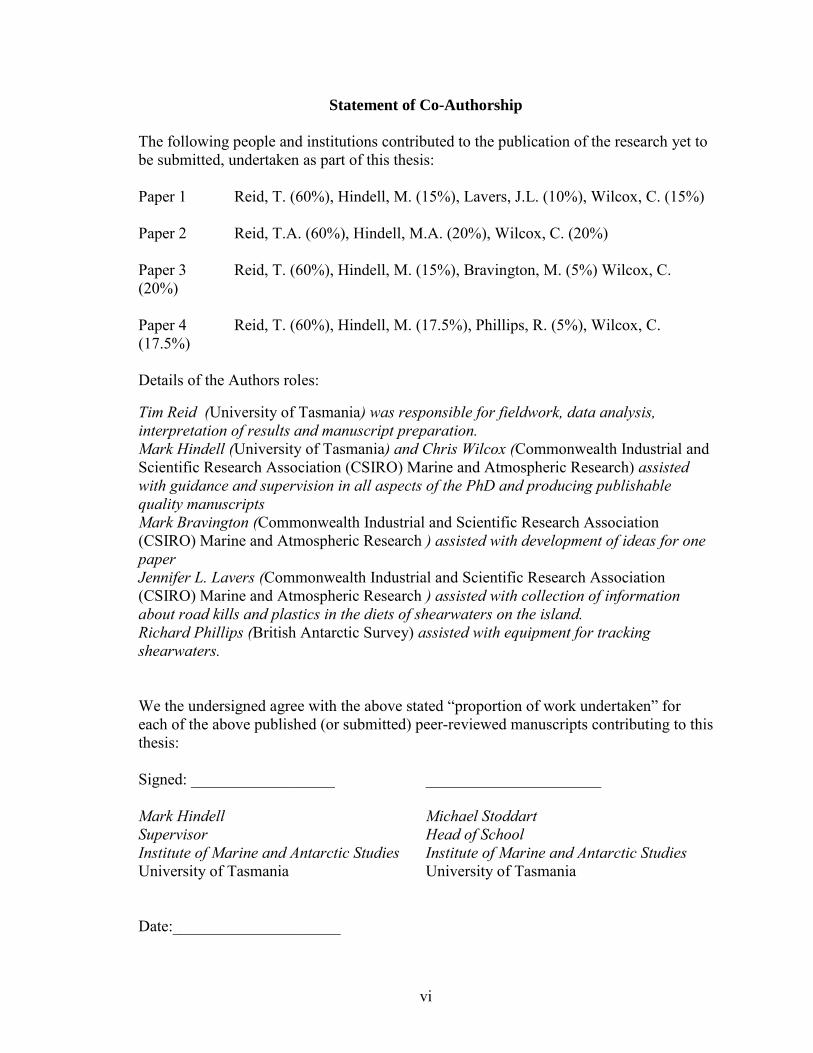
The following people and institutions contributed to the publication of the research yet to be submitted, undertaken as part of this thesis: Paper 1 Reid, T. (60%), Hindell, M. (15%), Lavers, J.L. (10%), Wilcox, C. (15%) Paper 2 Reid, T.A. (60%), Hindell, M.A. (20%), Wilcox, C. (20%) Paper 3 Reid, T. (60%), Hindell, M. (15%), Bravington, M. (5%) Wilcox, C. (20%) Paper 4 Reid, T. (60%), Hindell, M. (17.5%), Phillips, R. (5%), Wilcox, C. (17.5%) Details of the Authors roles: Tim Reid (University of Tasmania) was responsible for fieldwork, data analysis, interpretation of results and manuscript preparation. Mark Hindell (University of Tasmania) and Chris Wilcox (Commonwealth Industrial and Scientific Research Association (CSIRO) Marine and Atmospheric Research) assisted with guidance and supervision in all aspects of the PhD and producing publishable quality manuscripts Mark Bravington (Commonwealth Industrial and Scientific Research Association (CSIRO) Marine and Atmospheric Research ) assisted with development of ideas for one paper Jennifer L. Lavers (Commonwealth Industrial and Scientific Research Association (CSIRO) Marine and Atmospheric Research ) assisted with collection of information about road kills and plastics in the diets of shearwaters on the island. Richard Phillips (British Antarctic Survey) assisted with equipment for tracking shearwaters. We the undersigned agree with the above stated “proportion of work undertaken” for each of the above published (or submitted) peer-reviewed manuscripts contributing to this thesis: Signed: __________________ ______________________ Mark Hindell Michael Stoddart Supervisor Head of School Institute of Marine and Antarctic Studies Institute of Marine and Antarctic Studies University of Tasmania University of Tasmania Date:_____________________

vii

Acknowledgments And so the end of writing comes. Submitting to do a PhD is a wonderful experience; with

lots of ups and interesting things going on, learning and going to fantastic places. But of

coarse, there were downs as well (late nights sitting in my office trying to think of things

to write!). Overall though, it was really a lot of fun.

But anyway, I should thank people here. There are of coarse so many people to thank,

often for reasons that are trivial. Just being friends when you are struggling can be

enough. First and foremost to be thanked are my supervisors Chris Wilcox and Mark

Hindell, to both of whom I am incredibly grateful for all the advice and encouragement

that they have offered over the last few years. Thanks to Chris for helping with ways to

look at ecological perspectives in different ways, and to look at everything more

quantitatively. Both of them were always accessible when needed. So it has always been

a pleasure working with them.

Many other people have been given their time and helped me through this time. Richard

Coleman, Tom Trull and Denbeigh Armstrong from the QMS program at the University

of Tasmania were always helpful to the students and at times keeping us focused. Also

thanks to the other QMS students who have been there at times as well.

Simon Wotherspoon, Mark Bravington and Keith Hayes have helped with discussions

and statistical advice. Toby Patterson and Jim Dell have helped me with coding in Matlab

and using oceanographic data. Mike Sumner was equally helpful with R and methods of

dealing with tracking data. Scott Foster (CSIRO) assisted with fisheries data.

Dr David Priddel and Nicholas Carlisle of NSW Department of Climate Change gave me

a huge amount of useful advice initially and throughout the project. Nicholas Carlisle

assisted by giving positions for colony transects used in previous censuses. Barry Baker

provided many useful discussions about flesh-footed shearwaters and their status. Geoff

Tuck gave valuable information about the winter range. Ben Sullivan had many good

viii

discussions, some of which were useful. Richard Phillips offered useful discussions about

loggers and tracking birds.

Jennifer Lavers, Drew Lee, Peter Vertigan, Sam Thalmann, Michele Thums, Laurel

Johnston, Ray Murphy, Glen Dunshea, Rhonda Pike all assisted during field work on

Lord Howe Island. Lord Howe Island Board allowed accommodation at the Lord Howe

Island Research Facility. Thanks also to all of the fellow researchers who stayed there

and offered friendship and good discussions while we stayed in our small bit of paradise.

Christo Haselden, Hank Bowers and Sue Bowers assisted with work around Lord Howe

Island, and with colony area measurements. Fitzy helped with keeping me up to date with

Lord Howe Island gossip. The people in the AWRU lab was helpful in so many ways;

Mary-Anne Lea, Megan Tierney, Virginia Andrews-Goff, Andrea Walters, Susan Gallon,

Ben Arthur, Owen Daniel, Caitlin Vertigan and Ruth Casper. Richard Holmes assisted by

making a burrowscope.

Throughout my candidature I was supported by an Australian Government Postgraduates

Award and a joint University of Tasmania and CSIRO scholarship. The Commonwealth

Department of Environment, Heritage and Arts and CSIRO Wealth from Oceans Flagship

supplied funding for equipment and transport and accommodation on Lord Howe Island.

Fisheries data was supplied by the Australian Fisheries Management Authority (AFMA),

and remote sensing data was supplied by the Commonwealth Scientific and Industrial

Research Organisation (CSIRO). NCEP reanalysis data provided by the NOAA-CIRES

Climate Diagnostics Center, Boulder, Colorado, USA, from their Web site at

http://www.cdc.noaa.gov/.

Work on shearwaters was conducted under the University of Tasmania Animal Ethics

Committee Project number A0009154 and New South Wales Department of Climate

Change permit number S12408.

ix

Contents

Abstract ......................................... iii Statement of publication and co-authorship .................. v Acknowledgments .................................. vii Contents .......................................... ix

1. General Introduction .......................... 1

Conservation biology as a scientific discipline ........................................................... 1 Threats to marine predators ......................................................................................... 1 Fisheries ...................................................................................................................... 3 Fisheries waste ............................................................................................................ 3 Fisheries by-catch ........................................................................................................ 4 Pelagic long-line fishing impacts ................................................................................ 4 Flesh-footed shearwaters ............................................................................................. 5 Foraging ...................................................................................................................... 7 Aims ............................................................................................................................ 8 Population estimate and trend ..................................................................................... 8 Overlap with the ETBF ............................................................................................... 9 Fine scale attendance of ETBF vessels by shearwaters .............................................. 9 Individuals foraging distribution ................................................................................. 9 Thesis structure ......................................................................................................... 10

2. Status and trends of Flesh-footed shearwaters on

Lord Howe Island. ............................... 11

ABSTRACT ................................................................................................................. 12 INTRODUCTION ....................................................................................................... 13 METHODS .................................................................................................................. 16

Census of breeding colonies ...................................................................................... 16 Estimating road-kill ................................................................................................... 21 Data analysis ............................................................................................................. 22

RESULTS ..................................................................................................................... 23 Census ....................................................................................................................... 23 Burrow productivity .................................................................................................. 24 Number of chicks ...................................................................................................... 26 Breeding Success....................................................................................................... 27 Estimates of Road-kill ............................................................................................... 28

DISCUSSION .............................................................................................................. 30 Fisheries interactions and population trends ............................................................. 31 Onshore development and population trends ............................................................ 32 Marine debris............................................................................................................. 32 Road mortality ........................................................................................................... 33

x

CONCLUSION ............................................................................................................ 33 ACKNOWLEDGEMENTS ........................................................................................ 35

3. Environmental determinants of the at-sea

distribution of encounters between flesh-footed

shearwaters Puffinus carneipes and fishing vessels

................................................ 36


Data sources. ............................................................................................................. 43 Data Analysis. ........................................................................................................... 44

RESULTS. .................................................................................................................... 47 Modelling shearwater counts. ................................................................................... 48 Model validation ....................................................................................................... 50 Predicting distribution from AFMA data .................................................................. 52

DISCUSSION .............................................................................................................. 56 Using models as explanatory tools ............................................................................ 56 Using models as predictive tools ............................................................................... 58

CONCLUSIONS ......................................................................................................... 61 ACKNOWLEDGMENTS .......................................................................................... 62

4. Extracting information from incidental

observation data: using an arrivals-departures

multi-component model to quantify small scale

habitat use in a marine predator, the flesh-footed

shearwater. ..................................... 63


Data sources .............................................................................................................. 68 Model development ................................................................................................... 70 Model validation ....................................................................................................... 74 Estimating departure of individuals .......................................................................... 75 Model fitting .............................................................................................................. 75

RESULTS ..................................................................................................................... 76 Model validation ....................................................................................................... 76 Departure rates .......................................................................................................... 80 Model fitting .............................................................................................................. 80

DISCUSSION .............................................................................................................. 85 ACKNOWLEDGEMENTS ........................................................................................ 90

5. The importance of recent experience and

environment in determining large scale foraging

patterns in a pelagic seabirds, the flesh-footed

shearwater. ..................................... 91

ABSTRACT ................................................................................................................. 92 INTRODUCTION ....................................................................................................... 93

xi

METHODS .................................................................................................................. 96 Study site and species ................................................................................................ 96 Archival tag deployments.......................................................................................... 96 Estimation of at-sea movements ............................................................................... 98 Data analysis ............................................................................................................. 99 Kernel analysis .......................................................................................................... 99 Discrete Choice Models ............................................................................................ 99

RESULTS ................................................................................................................... 105 Discrete Choice Models .......................................................................................... 110 First Position ........................................................................................................... 110 Subsequent Positions ............................................................................................... 112

DISCUSSION ............................................................................................................ 116 CONCLUSIONS ....................................................................................................... 119 ACKNOWLEDGEMENTS ...................................................................................... 121

6. General Discussion and synthesis of results . 122

Population trend ...................................................................................................... 122 Spatial overlap with fisheries .................................................................................. 123 Foraging choices of shearwaters ............................................................................. 124 Foraging scale ......................................................................................................... 127 Management ............................................................................................................ 128 Marine protected areas ............................................................................................ 130 Marine protected areas and pelagic environments .................................................. 132

7. References .................................. 136

Chapter 1

1

1. General Introduction

Conservation biology as a scientific discipline

Conservation biology is concerned with the long-term viability of systems and preserving

biodiversity (Soulé 1985). Since the 1970‟s there has been increasing interest in the fields

of biodiversity and conservation biology due to the influence of human activity on

components of the natural environment (e.g. Soulé 1985; Costanza et al. 1997; Bowen

1999; Wood and Gross 2008). This increased interest has come from the recognition of

the importance of ecosystems, as well as the apparently increasing rates of extinction of

species (Soulé 1985). While there is growing importance placed on conserving

biodiversity, there remain issues of which taxonomic levels conservation should be

targeted, whether at conserving ecosystems, species, or identifiable genetic populations

(Bowen 1999). The human activities are diverse, from land clearing of forests for

agriculture to pollution of the atmosphere by industry.

There are a number of anthropogenic activities affecting the marine environment,

including benthic habitat destruction, overfishing, introduced species, global warming,

acidification, toxins and eutrophication due to runoff of nutrients. There is a general trend

of transforming once complex ecosystems into much more simple ones, such as replacing

coral reefs with muddy bottoms (Jackson 2001, 2008; Feely et al. 2004; Turner et al.

2008). In many areas, fish are being replaced by jellyfish as the dominant animals due to

overfishing (Richardson et al. 2008). Off Canada, overfishing of cod has lead to an

increase in urchins (which adult cod naturally eat), which in turn eat the kelp the juvenile

cod require for shelter (Myers and Worm 2005).

Threats to marine predators

Marine predators, especially those that spend time at the surface, being relatively

conspicuous, are useful for monitoring ecosystem health. Aspects such as their growth

rates or survival give useful measures of population health. This is especially true for

seabirds (Cairns 1987). A greater proportion of seabird species are declining than for any

Chapter 1

2

other groups of birds (Birdlife International 2008; Gonzalez-Solis and Shaffer 2009).

This indicates that many of these marine ecosystems are under stress. There are a range

of threats to seabird populations, including ingestion of plastics, pollution, introduced

predators on their colonies, habitat degradation (either at sea or on land) and fisheries

mortality (Croxall 1998).

A number of species of seabirds ingest plastics (e.g . Laysan albatrosses Phoebastria

immutabilis and flesh-footed shearwaters Aumann et al. 1998; Croxall 1998; Hutton et al.

2008). The plastics are ingested at sea being mistaken for food, and often much of it is

transferred to the chicks on the colony. Mortality of chicks due to plastics has rarely been

observed (Croxall 1998) but in some species there is a negative correlation between

plastic load and body condition (Connors and Smith 1982, Ryan 1987, Spear et al. 1995,

Auman et al. 1998).

Black-footed albatrosses Phoebastria nigripes from Hawai‟i have been shown to have

sufficiently high levels of organochlorines and DDT to be theoretically at risk of egg-

shell thinning and for this to have deleterious effects on embryos (Ludwig et al. 1998).

These chemicals are widely used in pesticides including in south and south-east Asia

(Croxall 1998). Seabirds and seals can become entangled in plastic packaging (Laist

1987).

Introduced predators affect a number of seabird species. Many species breed on islands

that have no native mammalian predators, and therefore have no evolved defences.

Mammals have been introduced to islands deliberately (for agriculture or as a food source

for ship wrecked sailors) or accidentally from ships. Pigs on Inaccessible Island have

affected the productivity of Wandering albatrosses Diomedea exulans (Ryan et al. 1990).

Mustelids need to be controlled around colonies of northern royal albatrosses Diomedea

sanfordi (Robertson 1998). More commonly, cats Felis catus, rats Rattus sp. and mice

Mus musculus have been implicated in seabird conservation. Cats prey on adult and chick

seabirds such as petrels and shearwaters, while rats and mice predate chicks and eggs

(McChesney and Tershy 1998; Cuthbert and Hilton 2004; Wanless et al. 2007; Le Corre

Chapter 1

3

2008; Rayner et al. 2008). Elimination of these predators from breeding colonies is likely

to be beneficial, however it may be complicated by interactions between these predators,

such as cats acting as mesopredators and controlling rats so that the removal of cats has in

places increased the declines in seabird populations (Courchamp et al. 1999; Rayner et al.

2008). Problems such as these emphasise the need for greater understanding of all the

threats to populations and how they interact with the ecology of the species being saved.

Habitat destruction can threaten seabirds either on their breeding colonies or at sea. Large

introduced mammals such as cattle Bos primigenius, sheep Ovis aries and goats Capra

hirca can damage breeding grounds through trampling (Croxall 1998; McChesney and

Tershy 1998), while humans can destroy breeding grounds for agriculture and residential

requirements (Priddel et al. 2006). Degradation of habitat at sea occurs through factors

such as pollution and climate change (Croxall 1998). These cause foraging areas to

decline in value either through a reduction of food at those areas or by causing the

conditions that usually predominate in the foraging areas to move.

Fisheries

Fisheries waste

Fisheries affect seabirds either through overfishing, which can change what resources are

available to seabirds, or through direct mortality of seabirds. Overfishing for sandeels

Ammodytes marinus in the North Sea has affected the population and breeding success of

seabirds such as the Arctic tern Sterna paradisaea and black-legged kittiwakes Rissa

tridactyla (Monaghan 1992; Frederiksen et al. 2004). Fisheries offal can change the

balance between seabird species (Oro and Martiez-Vilalta 1994; Furness 2003). Fisheries

waste can also provide food to seabirds (Thompson and Riddy 1995; Oro et al. 1995),

though this may not be of a high quality suited to successful breeding (Grémillet et al.

2008).

Chapter 1

4

Fisheries by-catch

Fisheries by-catch has been implicated in the declines of a number of species of seabird

(e.g. Croxall et al. 1990; Weimerskirch et al. 1997; Nel et al. 2002; Lewison and Crowder

2003). Mortality occurs in a number of fisheries, including long-lining (pelagic and

demersal), gill-netting (high-seas and coastal) and trawling (pelagic and demersal)

(Brothers 1991; DeGange et al. 1993; Sullivan et al. 2006a; Watkins et al. 2008). A

number of methods have been developed for mitigation of seabird mortality in fisheries.

These have included methodological approaches (such as fishing at night, or area

closures) and technological (changing equipment). Many of the mitigation measures

appropriate for one fishery have been adopted for others (with necessary adjustment for

the fishery methods used) (Brothers et al. 1999; Sullivan et al 2006b).

Pelagic long-line fishing impacts

Pelagic long-line fishing is a common method for targeting a range of finfish and sharks

(Tuck et al. 2003; Baker and Wise 2005), particularly large predatory fish such as tuna

Thunnus spp. and swordfish Xiphius gladius. The technique is used widely both for

coastal fisheries (which typically set hundreds of hooks), to high seas vessels setting

thousands of hooks. Pelagic long-lines consist of a mainline (which acts as a type of

backbone) set between a series of floats. This mainline may be up to 100 km long, with a

series of baited hooks attached to the mainline at regular intervals by 10-40m branchlines

(O‟Toole and Molloy 2000). These baited hooks are floated at depths depending on the

target species. For example lines targeting swordfish are frequently set with the hooks

less than 50m below the surface, while lines targeting bigeye or bluefin tuna may be up to

300m depth. Lines are set by a vessel feeding the line out behind it to be left floating for

some time (generally 4-6 hours; Tuck et al. 2003). The vessel then returns and retrieves

the line, hooks and catch. The setting and retrieving usually takes approximately 24

hours. These lines may have up to 3,000 baited hooks set on them (Tuck et al. 2003).

Chapter 1

5

The major cause of seabird mortality in pelagic long-line fisheries is due to the seabirds

(notably procellariiforms) taking baited hooks as the hooks are set behind the boat

(Brothers et al. 1999). A variety of technological and methodological techniques have

been developed to mitigate seabird by-catch in pelagic long-line fisheries (Brothers et al.

1999). Most distract seabirds from the baited hooks as they are set, or set the baited hooks

so that seabirds are unaware of them. Bird lines, which are aerial streamer lines that flap

erratically over the area that the bait are hitting the surface of the sea and initially sinking,

or attaching lead weights to the branch line to make the baited hook sink more rapidly so

that it is no longer within reach of the birds (Brothers et al. 1999). Methodological

techniques include dying bait blue (so they are less visible from above) or setting hooks

at night (when most species of seabirds are less active) (Brothers et al. 1999; Gilman et

al. 2007a). Baits are vulnerable to seabirds in the initial period of line setting, when they

are less than 5 m below the surface. Most of the mitigation methods have been designed

with considerations of albatrosses, which generally dive to depths of less than 10 m

(Brothers 1991; Prince et al. 1994; Brothers et al. 1999).

However, these standard techniques are not always effective. In pelagic long-line

fisheries, more manoeuvrable, deep diving species such as the petrels of the genus

Procellaria and shearwaters of the genus Puffinus are still caught in large numbers

despite these mitigation methods (Huin 1994; Baker and Wise 2005; Barbraud et al.

2008; Thalmann et al. 2009).

Flesh-footed shearwaters

The flesh-footed shearwater Puffinus carneipes is a medium sized shearwater (550-800g)

breeding in the southern hemisphere (on islands around New Zealand, Lord Howe Island,

islands off southern Western Australia, and Illé St Paul in the southern Indian Ocean) and

migrating to the northern hemisphere for the austral winter (Marchant and Higgins 1990).

The Eastern Tuna and Billfish Fishery is a pelagic long-line fishery operating in the

Tasman Sea targeting a range of tuna and swordfish species. In this fishery, 12 million

hooks were set in 2003 (Baker and Wise 2005), with most vessels setting between 1,000-

Chapter 1

6

1,200 hooks per day (Baker and Wise 2005). The fishery has a problem with seabird by-

catch, with flesh-footed shearwater the most commonly caught species (Trebilco et al.

2010). Between 1998 and 2002 8,972-18,490 flesh-footed shearwaters were killed in this

fishery, at rates that were considered unsustainable for the species (Baker and Wise

2005). The Lord Howe Island population declined between 1978 and 2002 (Priddel et al.

2006).

Several of the standard technological methods (including bird lines, attached weights,

underwater setting devices) were trialled in this fishery at this time without success at

lowering seabird by-catch rates (Baker pers. comm.). An alternative approach may be

area closures (Thalmann et al. 2009). In this, some of an area that may be used by

fisheries is closed so that there are no longer interactions between the vessels in the

fishery, and the by-catch species. For example, over two years from 1999 over one

million square miles of waters around the Hawaiian Islands were closed to a pelagic long-

line fishery due to incidental mortality of sea turtles (Curtis and Hicks 2000; Gilman et al.

2007b). Closure of such large areas is extreme, and probably detrimental to the fisheries'

continued viability. Alternatives may be communication within the fleet to identify real-

time hot-spots (Gilman et al. 2006), which has been successfully adopted in several

fisheries in the US. However to be effective, it required strong economic incentives, for

interactions with the by-catch species to be rare events and for a large observer presence

(Gilman et al. 2006). A second alternative may be to close more targeted areas, which are

of particular importance to the birds. However, to have a more targeted area closure it is

necessary to improve our understanding of the areas foraging requirements of the by-

catch. By understanding these it may be possible to identify the areas the by-catch species

will go and hence where interactions with fisheries are likely to occur. If interactions

occur predominantly in these areas, this may allow area closures to be relatively focused.

Knowledge of oceanographic features associated with foraging may allow information on

how the areas may change with changing conditions. This may allow the use of dynamic

area closures.

Chapter 1

7

Foraging

Marine predators do not forage randomly over the ocean but forage in areas that are likely

to have increased productivity and so concentrations of their prey. These are often

associated with up-welling areas where nutrient rich bottom water moves closer to the

surface within the photic zone. Up-wellings occur due to the movement of currents in

oceans due to wind or tides. When currents interact with barriers, such as land,

underwater ridges, or other currents, they are re-directed, often to the surface. The

resultant increased productivity then propagates up the food web until there are

concentrations of prey for top predators. These concentrations may be relatively

predictable in time and position, or they may be ephemeral. In the Tasman Sea, a western

boundary current moves south along the east coast of Australia. Part way down, this splits

with the Tasman Front passing near Lord Howe Island, where the flesh-footed

shearwaters breed (Ridgeway and Dunn 2003). These currents drive strong

oceanographic features such as up-wellings (Ridgeway and Dunn 2003), and so there are

likely to be areas of increased productivity for the shearwaters. Areas of increased

productivity are likely to have increased prey, and therefore increased foraging

opportunities for the shearwaters. Hence they should have increased foraging efficiency

by locating these areas (Charnov 1976). Therefore increasing understanding of these

mechanisms has the potential to be useful for designing and using area closures. There

are a number of alternatives for locating areas of prey concentrations. Several search

methods, such as the use of correlated random walks, Levy flights or area restricted

searches have been shown as increasing the efficiency of patches in an uneven

environment (Viswanathan et al. 1996; Fauchald and Tveraa 2003; Trembley et al. 2007).

An alternative is to use previous experience. For a central place forager, it is

advantageous to return to a patch that has previously been used successfully. This has

been demonstrated for a number of species, such as bumblebees and bluegill sunfish

(Werner et al. 1981; Peat and Goulson 2005). This is reliant to some extent on the patches

persisting so that they can be returned to. Areas of productivity (such as eddies) may be

dynamic, but may re-occur in approximately similar areas. Thus, it is possible that the use

of previous experience as well as efficient search methods would be beneficial to the

Chapter 1

8

searcher. If this occurs, it is likely that the shearwaters will return to approximately

similar areas. This may decrease the area necessary to be covered by area closures.

Aims

Increasing numbers of species are under threat, often through human activity. In this

thesis the threats to one species, the flesh-footed shearwater breeding on Lord Howe

Island, will be considered. This species has been shown to have been declining since the

1970‟s. To understand the threats to this population and how to manage them requires

increased information. Thus it is necessary initially to determine whether there are on-

going issues with the population of flesh-footed shearwaters, and if so, what they are.

Long-line fisheries by-catch has been a major issue for this species previously, while

previous technological attempts to mitigate this have so far been ineffective. It was

important therefore to examine spatial relations between the fishery and the foraging

range of the species. To do this it is important to examine the areas of overlap between

the fishery and the shearwaters, how this is changing over time and what effect this is

having on the by-catch rate, and to determine how shearwaters choose to forage where

they do. From this information consideration is given to how this may be useful toward

conservation, focussing on the use of dynamic area closures as potential ways to lower

the by-catch of this species. This thesis is organized into four research chapters and one

chapter drawing them together in a final synthesis.

Population estimate and trend

In Chapter 2 the current population of flesh-footed shearwaters on Lord Howe Island was

determined by conducting an island-wide census of the breeding colonies, and using

estimates of the colony size and density of burrows in conjunction with data on

occupancy and breeding success. Trends were determined by comparing the results of

this census to two past censuses. Possible threats apart from fisheries, such as plastics and

road mortality, were considered. Road mortality was estimated by calculating the density

of carcasses by the road and their rotting rate.

Chapter 1

9

Overlap with the ETBF

In Chapter 3 areas of attendance of vessels operating in the Eastern Tuna and Billfish

Fishery by flesh-footed shearwaters was quantified, using data from fisheries observers

on board vessels, logbook data and remote sensing data of oceanographic co-variates.

The areas of attendance were modelled, along with how these areas changed over the

period 1998-2006. The changes in vessel attendance were compared to changes in by-

catch rates in recent years. These changes in attendance with respect to area were used to

consider whether area closures are a potential method of conservation through changes in

the fisheries‟ locations affecting where interactions with the shearwaters occur.

Fine scale attendance of ETBF vessels by shearwaters

In Chapter 4 a novel statistical technique was used on the same data that was used in

Chapter 3. Flesh-footed shearwater attendance of long-line vessels was examined by

modelling their arrivals and departures between successive counts. Modelling these

activities and their co-variates allowed examination of fine scale attendance through the

changes in attendance with changes oceanographic conditions and activities of the

vessels. From this model a hypothesis that shearwaters were more likely to attend the

vessel when it is operating in good conditions was considered.

Individuals foraging distribution

Chapter 5 examines the at-sea distribution of individual flesh-footed shearwaters during

the breeding season using light-based archival tags (GLS loggers). Discrete Choice

Models were used to examine what cues were used by individuals to choose where they

were going during a foraging trips, and comparing the use of habitat variables such as

oceanography, and behaviour variables, such as experience. The use of previous

experience to locate potential foraging areas is thought to increase foraging efficiency,

either in comparison with, or in conjunction with other methods of searching. It has been

observed in some animals, but rarely in larger, and especially oceanic, animals. Discrete

Choice Models were used to make a quantitative examination of whether flesh-footed

shearwaters use experience.

Chapter 1

10

Thesis structure

This thesis has been written as a series of separate manuscripts with a number of co-

authors from the Antarctic Wildlife Research Unit, the British Antarctic Survey and

CSIRO Marine and Atmospheric Research. All chapters, with the exception of this

introductory and a final synthesis and summary chapter, consist of a series of manuscripts

either in preparation, or an already submitted paper for publication. As a consequence of

this layout, there is some overlap in ideas and text from each of these chapters. I was the

senior author each paper and so responsible for data analysis and interpretation and

preparation of the manuscripts, while the co-authors assisted with these. Co-authors are

listed with the chapter title at the start of each chapter. A single bibliography is presented

at the end of the thesis using Elsevier format (such as used in the journal Biological

Conservation).

Chapter 2

11

2. Status and trends of Flesh-footed shearwaters on

Lord Howe Island.

Tim Reid 1,2, Mark Hindell1, Jennifer L. Lavers 1,2 and Chris Wilcox 2.

1Institute of Marine and Antarctic Studies, Private Bag 129, University of Tasmania,

Sandy Bay, Tasmania, 7005, Australia 2Wealth from Oceans National Flagship, CSIRO Marine and Atmospheric Research,

GPO Box 1538, Hobart, Tasmania, 7001, Australia.

Chapter 2

12

ABSTRACT

The population of flesh-footed shearwaters breeding on Lord Howe Island have

previously been shown to be declining between the 1970‟s and the early 2000‟s. This was

shown to be predominantly due to the effect of breeding habitat clearance and fisheries

mortality in the Australian Eastern Tuna and Billfish Fishery. Recent evidence suggests

these influences have been reduced; therefore it was necessary to conduct a further census

of the population to establish on-going trends. Results presented here suggest there is an

85% probability that flesh-footed shearwaters on Lord Howe continued to decline during

2003-2009, and a number of possible reasons for this are suggested. During the breeding

season, road-based mortality of adults on Lord Howe Island is likely to result in reduced

adult survival and there is evidence that breeding success is negatively impacted by

marine debris. Interactions with fisheries on flesh-footed shearwater winter grounds and

should be further investigated.

Keywords: Flesh-footed shearwater, Lord Howe Island, population trends, Bayesian

analysis

Chapter 2

13

INTRODUCTION

Globally, marine vertebrates face a number of significant threats (Croxall and Gales

1998; Clover 2004). For example, in a number of regions the structure of ecosystems has

been altered by human-induced stresses such as overfishing, eutrophication or climate

change, with fish being replaced by jellyfish as the dominant animals (Richardson et al.

2009). Seabird species are declining at a faster rate than any other groups of birds

(Birdlife International 2008; Gonzalez-Solis and Shaffer 2009). The factors responsible

for the declines are varied and include increased adult mortality caused by fisheries,

effects of pollutants on fecundity and immunity, predation by introduced species, habitat

destruction, and the effects of climate change (Birdlife International 2008). Many

seabirds forage over a wide area and this brings them into contact with many impacted

areas/habitats. Seabirds are relatively long-lived animals that exhibit delayed breeding

and low fecundity, thus any additional adult mortality will have considerable

demographic consequences. This life-history strategy presents challenges for researchers

attempting to estimate population dynamics and manage multiple threats. While most

studies focus on individual threats to populations, a number of recent studies have

highlighted the need to consider multiple threats concurrently in order to improve our

understanding of the overall status of a population, and how best to conserve it (Wilcox

and Donlan 2007; Wanless et al. 2009). This can be most readily achieved with studies in

locations where some level of accuracy on the full range of threats can be obtained.

Flesh-footed shearwaters Puffinus carneipes (Gould 1844) are one of the most common

seabird by-catch (non-target mortality) species in long-line fisheries around Australia

(Gales et al. 1998; Baker and Wise 2005). The only colony of flesh-footed shearwaters

on Australia‟s east coast occurs on Lord Howe Island (Marchant and Higgins 1990),

which contains 5-14% of the total Australian population (Ross et al. 1996) and 8% of the

world‟s population (Brooke 2004). The Lord Howe Island population declined by 19%

(with an annual decline of 0.9%) between 1978- 2002 (Priddel et al. 2006). During 1998-

2002, an estimated 8,972-18,490 were killed in the Eastern Tuna and Billfish Fishery

(ETBF) (Baker and Wise 2005), leading to the perception that by-catch was the principal

factor driving the decline.

Chapter 2

14

In recent years, there has been a reduction in the observed by-catch rates, from 0.378

birds/1000 hooks between 1998 and 2002, to less than 0.07 birds/1000 hooks between

2002 and 2007 (Baker and Wise 2005; Lawrence et al. 2009). This decline in by-catch

rate has been attributed to the fishery moving north as the principle target species

changed from yellowfin tuna (Thunnus albacares Bonnaterre 1788) to albacore tuna (T.

alalunga Bonnaterre 1788).

A number of other issues may have contributed to the decline in the Flesh-footed

Shearwater population. First, the size of the breeding colonies on Lord Howe Island

declined by 36% between 1978-2002 due to land conversion for agricultural and

residential purposes (Priddel et al. 2006). Second, 79% of flesh-footed shearwater

fledglings contained plastic in their proventriculus on Lord Howe Island (Hutton et al.

2008), almost twice that of wedge-tailed shearwaters (P. pacificus Gmelin 1789) breeding

on the same island. However, it is unclear what the effect of the plastic was on the

survival of the chicks. And finally, several roads pass through or adjacent to flesh-footed

shearwater breeding colonies, and dead adults and fledglings are frequently found along

the roadsides (DECC 2009).

The flesh-footed shearwater is listed by the Australian Environmental Protection,

Biodiversity and Conservation (EPBC) Act as migratory under the JAMBA (Japan

Australia Migratory Bird Agreement) and ROKAMBA (Republic of Korea Australia

Migratory Bird Agreement) agreements (DEWHA 2009), and in New South Wales it is

currently listed as Vulnerable (DECC 2009). The flesh-footed shearwater was recently

identified as a strong candidate for inclusion under the international Agreement on the

Conservation of Albatross and Petrels (ACAP; Cooper and Baker 2008).

Because only two censuses of the Lord Howe Island flesh-footed shearwater population

have been undertaken, it is impossible to know if the observed declining trend between

those two observations is on-going and hence, whether management action is required

(Priddel et al. 2006; Tuck and Wilcox 2008). Tuck and Wilcox (2008) recently performed

Chapter 2

15

an Integrated Assessment Model on the status of flesh-footed shearwaters on Lord Howe

Island. The identified a number of issues with the model, as there was only data on two

threats to the shearwaters, while a number of others were identified. In light of the

changing by-catch rates, the aim of this paper is to quantify the current status of the Lord

Howe population and to increase the data available for a number of other threats

identified.

Chapter 2

16

METHODS

Lord Howe Island is a small (1,455 ha) volcanic island located approximately 495 km

east of Australia (Priddel et al. 2006). The island is crescent shaped with a coral reef on

the western side. At each end of the island there are volcanic mountains, with the

southern ones rising to 875 m. These are separated by an area of lowlands derived from

coral-derived calcarinite (Priddel et al. 2006). Much of this lowland area has been

developed for agriculture and settlement. For details of vegetation communities on the

island see Pickard (1983).

Flesh-footed shearwaters are a medium sized shearwater, weighing between 550-750 g

(Marchant and Higgins 1991). They breed on a number of islands in the southern

hemisphere, around New Zealand, in southern Western Australia, on Lord Howe Island,

and on Ílle Saint-Paul in the Indian Ocean, and migrate to the northern hemisphere for the

Austral winter, concentrating in the Arabian Sea (Powell 2009) and Sea of Japan. On

Lord Howe Island flesh-footed shearwater breed in lowland areas, predominantly in

sandy soil under palm forests on the eastern side of the island. There are currently five

discrete colonies on the eastern side (Ned‟s Beach, Steven‟s Point, Middle Beach, Clear

Place and Little Muttonbird Ground), with a small number also breeding in a single

colony on the western side (Hunter Bay) (Fig 1). Flesh-footed shearwaters are not known

to breed on any of Lord Howe‟s offshore islands (Priddel et al. 2006).

Census of breeding colonies

The census method was similar to that used by Priddel et al. (2006). The area of each

colony was measured by walking the perimeter with a hand held GPS (Magellan

Professional Mobile Mapper 6).

Chapter 2

17

Fig 2.1. Map of Lord Howe Island with location of flesh-footed shearwater breeding

colonies and roads. Positions of stations used for estimating breeding success marked as

circles.

The density of burrows within each colony was estimated using straight-line transects

through each colony on the island (except Hunter Bay where it was possible to count all

burrows). The transects used in this study were previously identified by Priddel et al.

(2006). Transects were evenly separated and oriented perpendicular to the longest axis of

the colony, passing from the colony edge to the centre of the colony. Transects were

divided into 10 meter sections, all burrows within two meters of either side of the transect

were counted. Apparent burrows were scored when they were judged to be large enough

for a flesh-footed shearwater to enter (>10 cm long). Based on this survey design, data

were divided into 40 m2 sections for analysis. The data were treated as count data, with

the total number of burrows per section as the response variable for statistical analysis.

Fitted values for the number of burrows per transect section were then used to estimate

0 2 km

Hunter Bay

Ned's Beach Steven's Point

Clear Place

Middle Beach

0 < deg

Chapter 2

18

standardized burrow density. Burrow counts were made between 29 October and 5

November 2008, after burrow cleaning had commenced but before egg-laying.

The number of burrows in each colony was estimated by calculating the mean (+s.d.)

density of burrows in each colony from the transect counts, and multiplying that by the

colony area (eqn. 1). The variance calculated during the estimate of burrow density was

then used to estimate confidence limits.

1

Pr{ }!

i

i i

y

B A B

eBi by

Equation 1.

Where A is the area of each colony i, B is the total number of burrows and is the density

of each colony i.

A number of burrows within the Clear Place colony have been studied regularly since

2005, and were used to quantify burrow occupancy rates. This was used to give a

measure of what proportion of burrows are occupied during a year, as not all burrows are

occupied every year. From this, the number of eggs laid, and hence the number of

breeding pairs, can be estimated. Burrows in this study colony were examined using a

custom-made burrowscope (Hamilton 1998) in early January each year. As egg laying

occurs in early December, it is likely that the estimate obtained here is a slight

underestimate. Burrows in the study colony were again examined in early April to check

for fledgling chicks. Breeding success (the number of eggs that produced chicks) was

estimated from this colony for each year. A small number of burrows were found in April

to contain chicks that had not been found to have eggs in January; this was adjusted for

using methods outlined by Priddel et al. (2006).

Burrow productivity gives an estimate of how many chicks are produced on Lord Howe

Island each year. This was measured by checking for the presence of chicks in a sample

Chapter 2

19

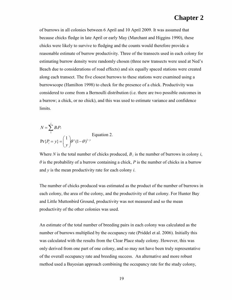
of burrows in all colonies between 6 April and 10 April 2009. It was assumed that

because chicks fledge in late April or early May (Marchant and Higgins 1990), these

chicks were likely to survive to fledging and the counts would therefore provide a

reasonable estimate of burrow productivity. Three of the transects used in each colony for

estimating burrow density were randomly chosen (three new transects were used at Ned‟s

Beach due to considerations of road effects) and six equally spaced stations were created

along each transect. The five closest burrows to these stations were examined using a

burrowscope (Hamilton 1998) to check for the presence of a chick. Productivity was

considered to come from a Bernoulli distribution (i.e. there are two possible outcomes in

a burrow; a chick, or no chick), and this was used to estimate variance and confidence

limits.

1

11Pr{ } (1 )

i

i i

y yi

N B P

P yy

Equation 2.

Where N is the total number of chicks produced, Bi is the number of burrows in colony i,

θ is the probability of a burrow containing a chick, P is the number of chicks in a burrow

and y is the mean productivity rate for each colony i.

The number of chicks produced was estimated as the product of the number of burrows in

each colony, the area of the colony, and the productivity of that colony. For Hunter Bay

and Little Muttonbird Ground, productivity was not measured and so the mean

productivity of the other colonies was used.

An estimate of the total number of breeding pairs in each colony was calculated as the

number of burrows multiplied by the occupancy rate (Priddel et al. 2006). Initially this

was calculated with the results from the Clear Place study colony. However, this was

only derived from one part of one colony, and so may not have been truly representative

of the overall occupancy rate and breeding success. An alternative and more robust

method used a Bayesian approach combining the occupancy rate for the study colony,

Chapter 2

20

and those from Priddel et al (2006). Using a Bayesian approach allows the combining of

all previous information into the one framework for estimating the number of breeding

pairs (McCarthy 2007). This allows the confidence that is held at each step in the process

of making the estimate to be incorporated into the final estimate.

The mean population estimate is calculated by multiplying the occupancy rate by the

colony area, as would have been done in a standard technique (the likelihood in Bayesian

terms). However a Bayesian approach adopts a formal method to update this estimate

with further information. This is done by multiplying the likelihood by a term (the prior),

to give a posterior estimate. How much this posterior differs from the likelihood depends

on the strength of the prior (which is dependent on the belief of the observer). Thus, if the

observer has no particular prior belief, an uninformative prior can be used (which will

essentially give a result similar to that found using standard statistical methods). In

Bayesian modelling it is generally not possible to come to an analytical version of the

sampling distribution; however this can be overcome using numerical methods (most

commonly the Monte Carlo Markov Chain) (McCarthy 2007).

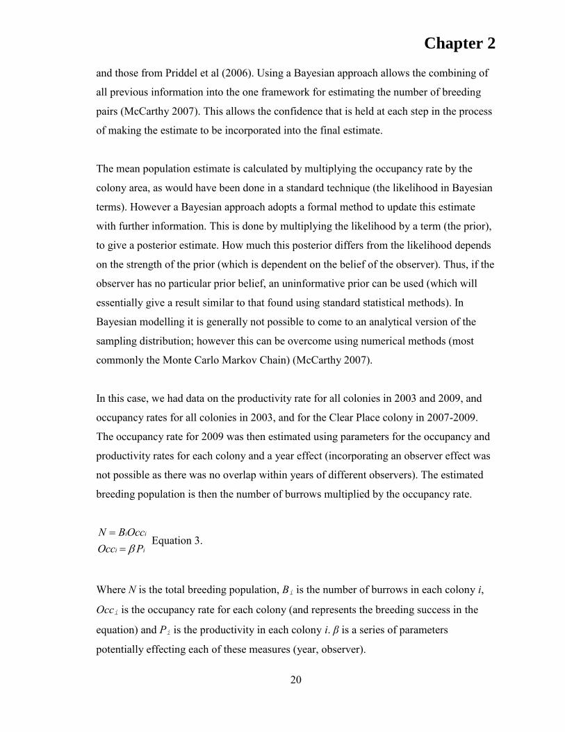
In this case, we had data on the productivity rate for all colonies in 2003 and 2009, and

occupancy rates for all colonies in 2003, and for the Clear Place colony in 2007-2009.

The occupancy rate for 2009 was then estimated using parameters for the occupancy and

productivity rates for each colony and a year effect (incorporating an observer effect was

not possible as there was no overlap within years of different observers). The estimated

breeding population is then the number of burrows multiplied by the occupancy rate.

i i

i i

N B OccOcc P

Equation 3.

Where N is the total breeding population, Bi is the number of burrows in each colony i,

Occi is the occupancy rate for each colony (and represents the breeding success in the

equation) and Pi is the productivity in each colony i. β is a series of parameters

potentially effecting each of these measures (year, observer).

Chapter 2

21

Estimating road-kill

The density of carcass was measured along three roads passing through or beside a

colony (Ned‟s Beach Road at Ned‟s Beach, Skyline Drive and Muttonbird Drive by

Steven‟s Colony) by walking 10 m transects at right angles from the road, counting all

carcasses within 1 m of either side of the transect. Ten evenly spaced transects were made

along Skyline and Muttonbird Drives, and 20 evenly spaced along Ned‟s Beach Road (all

approximately 10 m apart).

Seven carcasses were marked on 1 January 2008 to determine how long carcases would

be detectable in the forest beside the road until they were re-checked in early April 2008.

Using this rate of disappearance and assuming that road mortalities occurred at an

approximately even rate throughout the summer, it is possible to estimate an approximate

maximum for the number of carcasses required to end with the number located on the

transects in April 2009 using Equation 4.

2

0

0

( )

( )

( ) (1 )

(1 )

( )

t

tt

t dt

X P X

f t f

N N e

E C X D

PX p p

X

E C E C P

Equation 4.

Where N is the total number of carcasses killed on the roads, λ is the rate of

disappearance of corpses, t is the days from 0 to i, d is the daily probability of death, P is

the total number of shearwaters available on the island to be run over, p is the probability

of shearwaters dying, X is the rate of birds dying, E(Ct) is the expected number of

corpses, E(Cf) is the expected corpses found and Pf is the probability that a corpse will be

found.

Chapter 2

22

Data analysis

A model-based approach, rather than a design-based estimate, was used to estimate the

mean and variance in occupancy and productivity in this study. Data analysis was

performed using R statistical software (version 2.9.0 R Foundation for Statistical

Computing 2009). Bayesian analyses were performed using WinBUGS (version 1.4,

Lunn et al. 2000).

Chapter 2

23

RESULTS

Census

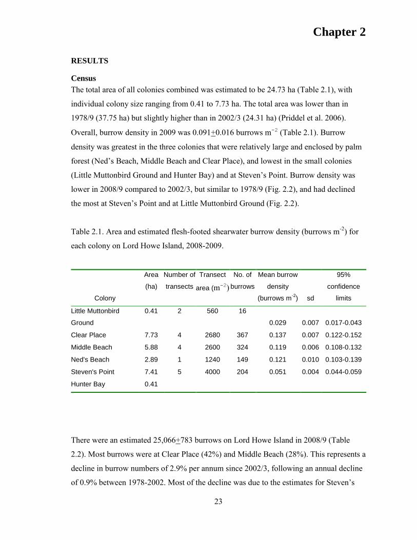
The total area of all colonies combined was estimated to be 24.73 ha (Table 2.1), with

individual colony size ranging from 0.41 to 7.73 ha. The total area was lower than in

1978/9 (37.75 ha) but slightly higher than in 2002/3 (24.31 ha) (Priddel et al. 2006).

Overall, burrow density in 2009 was 0.091+0.016 burrows m-2 (Table 2.1). Burrow

density was greatest in the three colonies that were relatively large and enclosed by palm

forest (Ned‟s Beach, Middle Beach and Clear Place), and lowest in the small colonies

(Little Muttonbird Ground and Hunter Bay) and at Steven‟s Point. Burrow density was

lower in 2008/9 compared to 2002/3, but similar to 1978/9 (Fig. 2.2), and had declined

the most at Steven‟s Point and at Little Muttonbird Ground (Fig. 2.2).

Table 2.1. Area and estimated flesh-footed shearwater burrow density (burrows m-2) for

each colony on Lord Howe Island, 2008-2009.

Colony

Area

(ha)

Number of

transects

Transect

area (m-2) No. of

burrows

Mean burrow

density

(burrows m-2

) sd

95%

confidence

limits

Little Muttonbird

Ground

0.41 2 560 16

0.029 0.007 0.017-0.043

Clear Place 7.73 4 2680 367 0.137 0.007 0.122-0.152

Middle Beach 5.88 4 2600 324 0.119 0.006 0.108-0.132

Ned's Beach 2.89 1 1240 149 0.121 0.010 0.103-0.139

Steven's Point 7.41 5 4000 204 0.051 0.004 0.044-0.059

Hunter Bay 0.41

There were an estimated 25,066+783 burrows on Lord Howe Island in 2008/9 (Table

2.2). Most burrows were at Clear Place (42%) and Middle Beach (28%). This represents a

decline in burrow numbers of 2.9% per annum since 2002/3, following an annual decline

of 0.9% between 1978-2002. Most of the decline was due to the estimates for Steven‟s

Chapter 2

24

Point and Clear Place, with marginally greater estimates of the number of burrows for

Ned‟s Beach and Middle Beach compared to 2002/3 (Fig. 2.3).

Fig 2.2. Burrow density (burrows m-2) at each colony on Lord Howe Island in three years

(error bars represent standard errors, as those are what was given in Priddel et al. 2006).

(1978=1978/9; 2002=2002/3; 2008=2008/9; SP=Steven‟s Point; MB=Middle Beach;

CP=Clear Place; NB=Ned‟s Beach; LMG=Little Muttonbird Ground; HB=Hunter Bay).

Burrow productivity

Burrow productivity was 0.359+0.102 chicks burrow-1 in 2009 (Table 2.3). Productivity

was highest at Clear Place, and lowest at Ned‟s Beach (Table 2.3). It was slightly higher

in 2008/9 than 2002/3, though not significantly. There was no consistent pattern between

colonies among years, though it was almost three times higher at Steven‟s Point in

2008/9 than in 2002/3 (Fig 2.4).

Burr

ow

density (

burr

ow

s/m

2)

0.0

00.0

50.1

00.1

50.2

00.2

5

SP MB CP NB LMG HB Total

1978

2002

2008

Chapter 2

25

Table 2.2. Estimated number of burrows for each colony on Lord Howe Island, 2008-

2009. Note all burrows counted at Hunter Bay.

Colony burrows sd 95% confidence limits

Little Muttonbird Ground 118 29 69-178

Clear Place 10588 568 9455-11720

Middle Beach 7001 369 6329-7750

Ned's Beach 3485 281 2970-4029

Steven's Point 3783 272 3269-4356

Hunter Bay 91

Total 25066 783 23532-26600

Fig 2.3. Estimated total number of burrows on Lord Howe Island in 1978/9, 2002/3

(Priddel et al. 2006) and 2008/9.

1980 1985 1990 1995 2000 2005

20000

30000

40000

Year

Estim

ate

d t

ota

l burr

ow

s

Chapter 2

26

Table 2.3. Estimated burrow productivity for each colony (fledglings burrow-1) on Lord

Howe Island, 2008-2009.

Colony Burrows checked occupied mean sd 95% confidence limits

Clear Place 90 39 0.435 0.052 0.333-0.540

Middle Beach 75 28 0.376 0.054 0.277-0.489

Ned's Beach 95 27 0.300 0.046 0.213-0.388

Steven's Point 85 30 0.358 0.052 0.262-0.465

Total 0.359 0.102 0.160-0.558

Fig 2.4. Burrow productivity (chicks burrow-1) at each colony in 2002/3 and 2008/9 (error

bars represent standard errors, as those are what was given in Priddel et al. 2006).

Number of chicks

An estimated 9,712+783 chicks were produced on Lord Howe Island in 2009 (Table 2.4).

Most chicks were produced in Clear Place (47%) and Middle Beach (27%). This is an 8%

increase in the estimated number of chicks produced compared with 2002/3, with most of

the increase due to an apparent doubling in the number of chicks produced at Steven‟s

Burr

ow

pro

ductivity (

chic

ks/b

urr

ow

)

0.0

0.1

0.2

0.3

0.4

0.5

0.6

Stevens Pt Middle Beach Clear Place Neds Beach Total

2002

2008

Chapter 2

27

Point (Priddel et al. 2006). On 27 January 2009 six adult flesh-footed shearwaters were

located within a wedge-tailed shearwater colony at Signal Point on the west coast, south

of Hunter Bay, where breeding had not previously been recorded. Breeding was not

confirmed at this location, but there was some evidence to suggest a small number of

nests present (<10) (pers. obs.). No other flesh-footed shearwaters were located in any of

the other nearby wedge-tailed shearwater colonies.

Table 2.4. Estimated number of chicks from each colony on Lord Howe Island, 2008-

2009.

Colony chicks sd 95% confidence limits

Little Muttonbird Ground 42 16 11-73

Clear Place 4607 609 3437-5833

Middle Beach 2631 402 1869-3448

Ned's Beach 1046 181 731-1447

Steven's Point 1354 218 946-1829

Hunter Bay 33 9 15-51

Total 9713 783 8177-11248

Breeding Success

Breeding success (eggs that produced chicks that were likely to fledge) was estimated in

Clear Place for three years (2006/7, 2007/8 and 2008/9) (Table 2.5). Using the Bayesian

model to combine these figures with those derived from Priddel et al. (2006), breeding

success in 2009 was estimated at 0.55 (95% confidence limits 0.42-0.78).

Chapter 2

28

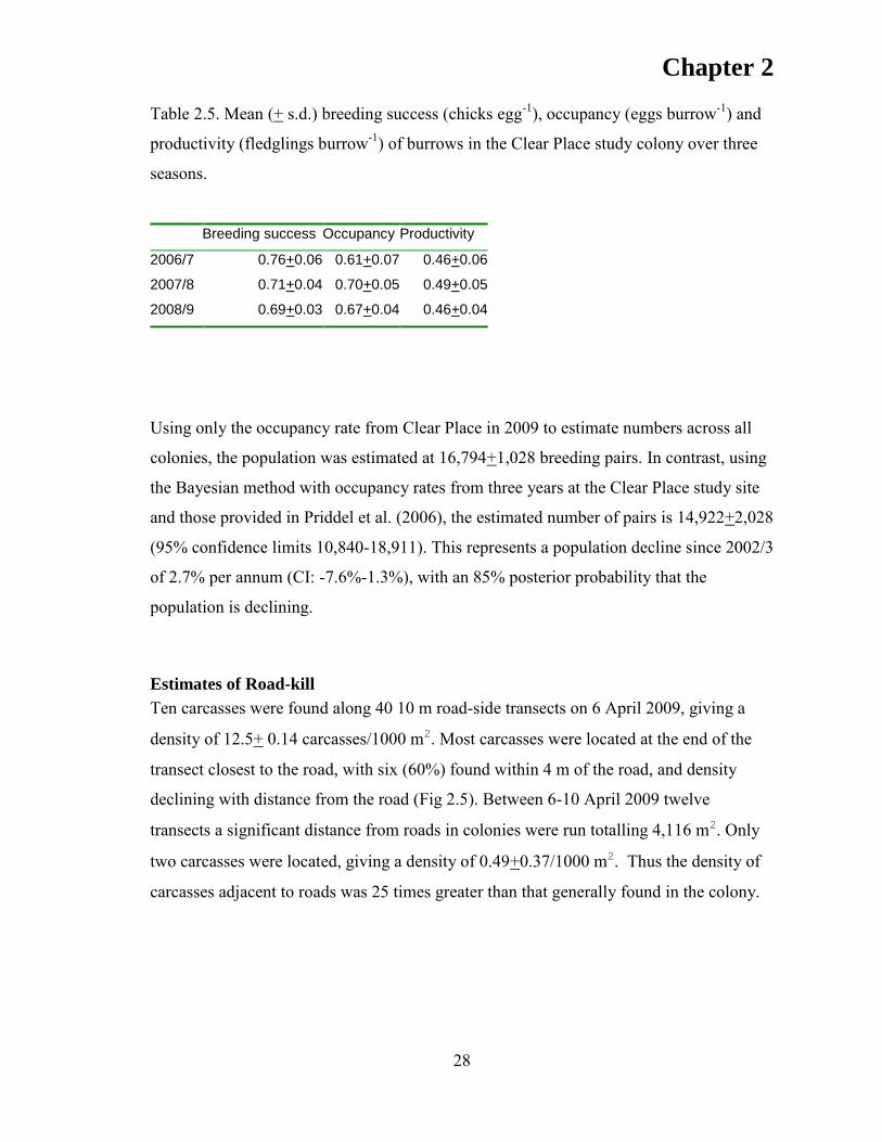
Table 2.5. Mean (+ s.d.) breeding success (chicks egg-1), occupancy (eggs burrow-1) and

productivity (fledglings burrow-1) of burrows in the Clear Place study colony over three

seasons.

Breeding success Occupancy Productivity

2006/7 0.76+0.06 0.61+0.07 0.46+0.06

2007/8 0.71+0.04 0.70+0.05 0.49+0.05

2008/9 0.69+0.03 0.67+0.04 0.46+0.04

Using only the occupancy rate from Clear Place in 2009 to estimate numbers across all

colonies, the population was estimated at 16,794+1,028 breeding pairs. In contrast, using

the Bayesian method with occupancy rates from three years at the Clear Place study site

and those provided in Priddel et al. (2006), the estimated number of pairs is 14,922+2,028

(95% confidence limits 10,840-18,911). This represents a population decline since 2002/3

of 2.7% per annum (CI: -7.6%-1.3%), with an 85% posterior probability that the

population is declining.

Estimates of Road-kill

Ten carcasses were found along 40 10 m road-side transects on 6 April 2009, giving a

density of 12.5+ 0.14 carcasses/1000 m2. Most carcasses were located at the end of the

transect closest to the road, with six (60%) found within 4 m of the road, and density

declining with distance from the road (Fig 2.5). Between 6-10 April 2009 twelve

transects a significant distance from roads in colonies were run totalling 4,116 m2. Only

two carcasses were located, giving a density of 0.49+0.37/1000 m2. Thus the density of

carcasses adjacent to roads was 25 times greater than that generally found in the colony.

Chapter 2

29

Fig 2.5. Number of flesh-footed shearwater carcases along 10 m transects perpendicular

to roads on Lord Howe Island (only those roads through colonies were observed).

Seven flesh-footed shearwater carcasses that were killed on Ned‟s Beach Road on the

night of 31/12/2007 were marked. Four of these were still easily identifiable on

17/4/2008, indicating that the carcasses last for at least 3.5 months. Three had

disappeared, presumably due to break down or being buried.

Assuming that all carcasses are detectable throughout a breeding season (this needs to be

tested) and that all birds hit by cars die within 10 m of a road, using the density of

carcasses within 10 m of the road edge for the length of the roads on Lord Howe Island,

produces an estimate of 125 birds killed during the 2008/2009 breeding season. In

comparison, using the background density recorded throughout the rest of the colony,

multiplied by the colony size, there would be 121 carcasses by natural mortality. This

suggests that the road mortality may be doubling natural mortality within the colony.

Alternatively, using the assumptions of Equation 4 (a constant rate of mortality and of

carcass disappearance) to estimate road mortality, it is estimated 185 (C.I. 129-262) birds

were killed on the roads.

0-2 2-4 4-6 6-8 8-10

Distance from road (m)

Num

ber

of

carc

asses

0.0

0.5

1.0

1.5

2.0

2.5

3.0

Chapter 2

30

DISCUSSION

Recently there has been an apparent reduction in the observed mortality of flesh-footed

shearwaters on long-line fishing vessels in the ETBF off eastern Australia (Baker and

Wise 2005; Lawrence et al. 2009). Flesh-footed shearwaters are considered Vulnerable in

New South Wales, as the only breeding colony (Lord Howe Island) has been declining

since 1978 (Priddel et al. 2006), and it is likely that the majority of flesh-footed

shearwaters still taken in the ETBF each year originated on Lord Howe Island due to the

proximity of the fishery to the island. Because fisheries mortality was considered one of

the major causes of this decline, we conducted a census of the population on Lord Howe

Island to estimate the most recent population trends.

The estimated number of burrows within all of the colonies on Lord Howe Island

declined at an annual rate of 0.9% during 1978-2002 (Priddel et al. 2006). The rate

increased to 2.9% during 2002-2008, giving an overall annual rate of decline in burrow

numbers of 1.3% since 1978. Correspondingly, the number of breeding pairs was

estimated to have declined by 2.7% per annum between 2002-2008. Overall there was a

14% decline in the estimated number of breeding pairs on Lord Howe Island between

2002-2008, though it was not significantly different from zero. Nevertheless, there is an

85% probability that the population had declined since 2002.

The decline in colony area between 1978-2002 (Priddel et al. 2006) seems to have halted

in recent years. Much of this decline was due to land being converted to residential or

agricultural uses, and management of the island has changed to reduce this (Priddel et al

2006). Despite this, there was still a decline in the overall number of burrows. This was

partly driven by the declining density of burrows in recent years, to a density similar to

that in 1978. The declines in burrow density were most noticeable in the smaller colonies

(Hunter Bay and Little Muttonbird Ground), and the colony most affected by

urbanization (Steven‟s Point). This trend was also noted by Priddel et al. (2006).

Overall, parameters for the larger colonies (Clear Place, Middle Beach and Ned‟s Beach)

have not changed greatly since 2002, with minimal changes observed at Clear Place and

Chapter 2

31

Ned‟s Beach since 1978 (Priddel et al. 2006). Middle Beach declined in area by 41%

between 1978 and 2002, with an 18% decline in the estimated number of burrows since

1978. This pattern of declines at the edges of colonies has been noted for other species

(e.g. Gochfeld 1980; Aebischer and Coulson 1990).

In this study a model-based approach using Bayesian statistical methods was adopted.

This method was preferred over design-based inferences for two reasons. First, the

modelling approach is better at accounting for sources of variation (Waugh et al. 2008).

The use of Bayesian methods presents a way to formally incorporate data and variation

from different sources into the estimate (McCarthy 2007). These methods were adapted

in the current study due to the availability of previous estimates of breeding success from

the Clear Place colony, which appeared to have consistently high success compared to

previous observations more generally throughout the island (Dyer 2001; Priddel et al.

2006). This allowed for previous estimates to adjust the estimates of the population for

2009, and to better reflect the uncertainty about this estimate.

Fisheries interactions and population trends

Observed fisheries mortality in the ETBF was significant between 1998-2002 (Baker and

Wise 2005), but has fallen drastically since 2002, therefore on-going declines are unlikely

to be related to this. However, there may still be mortality in flesh-footed shearwater‟s

wintering grounds. Flesh-footed shearwaters are known to migrate to the northern Pacific

Ocean, with sightings and band records from the Sea of Japan (Shuntov 1972, Tuck and

Wilcox 2008), east of Japan (Oka 1994; Ito 2002; Ogi 2008), and off western Canada

(Wahl et al. 1989; Hay 1992). While banding records originate from Lord Howe Island,

sightings may be of birds originating on Lord Howe, or alternatively, from colonies in

New Zealand or off Western Australia. In the past, significant numbers of flesh-footed

shearwaters have been taken as by-catch in a number of drift net fisheries in the north

Pacific Ocean. In 1987, 116 flesh-footed shearwaters were killed in a salmon drift net

fishery east of Japan (Degange and Day 1991), while in 1990 between 397-957 were

killed in neon flying squid drift net fisheries in the North Pacific (Ogi 2008). While these

high seas drift net fisheries have closed since the early 1990‟s, there continues to be a

Chapter 2

32

number of drift (gill) net fisheries operating in national waters, and these continue to pose

a potential threat to shearwaters. Japan operates a large coastal long-line fishery in the

waters to the east that potentially overlaps with the range of flesh-footed shearwaters

(Tuck and Wilcox 2008).

Onshore development and population trends

The loss of breeding habitat on Lord Howe Island was implicated in the flesh-footed

shearwater population decline during 1978-2002 (Priddel et al. 2006). The decline in

colony area seems to have ceased, with a slight increase in colony area noted and one

new colony detected in 2008. While the area of the colonies has not declined since 2002

and there has been little change in the three larger colonies, the number of burrows in the

smaller and more fragmented colonies has declined. This would suggest that edge effects

may be significant at those colonies. The areas with greatest burrow density are in sandy

soil under palm forests; at the edges of the colonies there are often intrusions of kikuyu

grass Pennisetum clandestinum, and other weeds from gardens or paddocks, and the

shearwaters find this difficult to burrow into (Priddel et al. 2006). This suggests that if

efforts are made to increase the area of breeding habitat, they would be best aimed at the

edges of existing colonies, especially Ned‟s Beach, Middle Beach and Clear Place, or if

possible, filling in gaps in colonies.

Marine debris

Fledgling flesh-footed shearwaters on Lord Howe Island contain significant quantities of

plastics that likely negatively influence chick body condition and thus, breeding success

(Hutton et al. 2008). Small numbers of adult flesh-footed shearwaters are killed each

year as a result of perforations to the digestive tract by plastic debris (unpublished data).

However, while there is substantial evidence that plastic load is negatively correlated

with body condition in seabirds (e.g., birds who ingest large amounts of plastic have low

fat reserves; Connors & Smith 1982, Ryan 1987, Spear et al. 1995, Auman et al. 1998),

direct (statistical), quantitative evidence of the negative effects of plastics in any seabird

species is lacking (Laist 1997, Robards et al. 1997).

Chapter 2

33

Road mortality

Flesh-footed shearwater carcasses were much more common along the edge of roads,

clearly demonstrating their vulnerability to traffic, with roads more than doubling natural

mortality on land. Traffic has been highlighted as a problem on Lord Howe Island since

the early 1970‟s (Recher and Clark 1974), and was recently identified as a significant

threat to flesh-footed shearwaters (DECC 2009). We have assumed here that the

carcasses recorded were from throughout the season, so that there was no loss of

carcasses from earlier in the summer. In 2008, detectability of carcasses declined

suggesting that the number of road mortalities may be much greater than that calculated

assuming they remain visible for the complete season. To assess this more accurately, it

would be necessary to mark a number of carcasses in order to follow their condition over

time, and use a more detailed assessment of the carcasses counted in the survey.

Nevertheless, 125 carcasses killed on the road represents an annual adult mortality of

approximately 0.2%. This mortality is up to 5 times that generated through by-catch in

the ETBF long-line fishery (Tuck and Wilcox 2008). Long-lived seabirds, such as the

flesh-footed shearwater, rely heavily on survivorship of breeding adults to maintain

population numbers (Croxall and Rothery 1991). Using the life expectancy (LE)

estimator formula LE = -1/ln(Φ), where Φ = annual survival, we can observe the

changes in life expectancy as a result of changes in the survival rate (Lack 1954). For

example, an adult flesh-footed shearwater with Φ = 0.92 will live to 28 years of age

while an adult with Φ = 0.918 would be expected to live only 22 years. Therefore, small

changes in the adult mortality greatly influence the growth of a population by reducing

both the lifespan and potential reproductive output of breeding adults.

CONCLUSION

Analysis of the flesh-footed shearwater population on Lord Howe Island showed an 85%

chance that it was continuing to decline between 2002-2008. Four factors have been

implicated in the decline; while habitat destruction and by-catch in the ETBF have

Chapter 2

34

previously been implicated they are currently no longer causing major issues. However

we have demonstrated that there is significant mortality on the roads of Lord Howe

Island, and that this may be sufficient to explain the continuing decline. There is evidence

of plastics in the stomachs of birds, especially chicks, however it is unclear what effect

this is having on the population and further investigation is warranted. Finally, flesh-

footed shearwaters winter in areas that potentially could interact with fisheries. At

present, flesh-footed shearwater by-catch in this region is poorly understood.

Chapter 2

35

ACKNOWLEDGEMENTS

Laurel Johnston and Drew Lee assisted in the field. Christo Haselden, Hank Bowers and

Sue Bowers assisted with colony area measurements. Nicholas Carlisle assisted with

setting up transects. Funding for TR was supplied by an Australian Government

Postgraduates Award and a joint University of Tasmania and CSIRO scholarship. The

University of Tasmania supplied a scholarship. Funding for JLL was provided by the

Commonwealth Environment Research Facilities Programme, Government of Australia

Endeavour Research Fellowship, and a Gould League of NSW Centenary 2010 Cayley

Memorial Scholarship. CSIRO and the Department of Environment, Water, Heritage and

Arts supplied additional funding.

Chapter 3

36

3. Environmental determinants of the at-sea

distribution of encounters between flesh-footed

shearwaters Puffinus carneipes and fishing vessels

Tim A. Reid1,2*, Mark A. Hindell1 and Chris Wilcox2.

1School of Zoology, University of Tasmania, Sandy Bay, Tas, 7000, Australia. 2CSIRO Marine and Atmospheric Research Laboratories, Hobart, Tas, 7000,

Australia.

Chapter 3

37

ABSTRACT

Fisheries observer data were used to model the distribution of seabird encounters for

identifying areas for fisheries closures. Data from the Eastern Tuna and Billfish Fishery

(ETBF) in the Tasman Sea (off the east coast of Australia) were used and the focal bird

species was the flesh-footed shearwater (the species most commonly killed in this

fishery).

Encounters between flesh-footed shearwaters and long-line fishing vessels varied with

season, distance from Lord Howe Island, and a number of environmental and

oceanographic variables (in particular, chlorophyll-A levels, wind speed, sea height and

bathymetry). Encounters were most common to the south-west of Lord Howe Island, in

waters associated with the Tasman Front and the East Australia Current.

The resulting model was used to predict the overlaps between fisheries and flesh-footed

shearwaters during three years (1997/1998, 2003/2004 and 2006/2007). During

2003/2004 the area predicted to have high interactions was also the area with high fishing

effort. During that year, there were also high mortalities of shearwaters in the fishery

(Trebilco et al. 2010). In 2006/2007 the main fishing effort was well to the north of areas

with predictions of high interactions. Seabird by-catch was low during that year. The

species of fish targeted by the majority of the fishery also changed between years. This

result illustrates that the most likely reason for falling by-catch rates in this fishery were

movements of the fishing effort to areas away from the birds, rather than changes in

fishing technique.

These results emphasise the potential of area closures as a method of by-catch mitigation

for species that are proving intractable for standard by-catch methods. The use of data

collected from fisheries vessels to identify characteristic areas of interactions is also

important. This would be improved with increasing data on the distribution of the

shearwaters.

Chapter 3

38

Keywords: flesh-footed shearwater, long-line fishing, by-catch, Lord Howe Island, at-sea

interactions

Chapter 3

39

INTRODUCTION

Worldwide, many seabirds are killed in commercial fisheries operations, in some species,

in sufficient numbers to adversely affect their conservation status (Bartle 1991; Brothers

1991; Nel et al. 2002; Sullivan et al. 2006a). Particular attention has concentrated on

albatrosses (e.g. Bartle 1991; Brothers 1991; Nel et al. 2002; Sullivan et al. 2006a),

however a number of species of shearwaters and petrels are also severely effected

(Brothers et al. 1999; Baker and Wise 2005; Phillips et al. 2006). Flesh-footed

shearwaters (Puffinus carneipes Gould 1844) are killed in significant numbers during

long-line fishing in the Eastern Tuna and Billfish Fishery (ETBF) off the east coast of

Australia (Baker and Wise 2005). The shearwaters killed in the fishery are thought to

come primarily from the Lord Howe Island population, and a modelling study has

suggested that the population cannot sustain the reported levels of mortality (Baker and

Wise 2005). This population has been shown to be declining since the 1970‟s (Priddel et

al. 2006).

A number of mitigation techniques have been used in fisheries to reduce this mortality,

including night-setting, line-weighting, and bird-lines; however, so far none have been

found to be effective with flesh-footed shearwaters in the ETBF (Lawrence et al. 2006).

Most methods of mitigation aim to reduce the impact of interactions once by-catch

species encounter fishing vessels (Brothers et al. 1999; Sullivan et al. 2006b), and these

methods can be less effective against deep diving or night foraging seabirds such as flesh-

footed shearwaters and white-chinned petrels (Brothers et al. 1999).

An alternative strategy may be to reduce mortalities by decreasing the number of seabirds

that encounter fishing vessels in the first place, for example by preventing fishing in areas

that have high numbers of seabirds. Seabird by-catch increases with abundance of

seabirds around fishing vessels, so avoiding areas with high concentrations of frequently

caught species of birds may provide a simple and effective measure (Lawrence et al

2006). However, to adopt this strategy, we need to improve our understanding of the at-

sea distribution of seabirds such as flesh-footed shearwaters, and the underlying factors

that determine it.

Chapter 3

40

Broadly speaking, there are two ways to quantify this; via telemetry (Shaffer et al. 2006),

or using observations of seabirds at sea (Reid et al. 2002, Camphuysen et al. 2004). Data

loggers and satellite tracking devices provide detailed information on (generally) small

numbers of individuals. The weight of the devices also limits the size of birds that can be

studied in this way, although with increasingly smaller devices the number of species that

can be studied is steadily increasing. The alternative, data from at-sea observations has

the advantage of being derived from larger numbers of birds. During fisheries operations,

counts of attending seabirds are frequently made for fisheries management purposes but

these data have rarely been used for looking at the distribution of the seabirds at sea, as

the data are considered to be biased because some species of seabirds (e.g. albatross) are

attracted to vessels, while others may avoid them (Hyrenbach 2001). Additionally,

fisheries observers generally have a number of other activities relating to fisheries

management, and so they do not have the time for using distance or area sampling

techniques (Spear et al. 2004).

However, if the data for a single species are used for answering well-targeted questions,

these issues are likely to be lessened. If a species is attracted to fishing vessels, counts of

that species can appropriately be used for quantifying their relative distribution, and the

likelihood of interaction with vessels. Seabirds, such as flesh-footed shearwaters, forage

over the ocean in a targeted, rather than a random, manner (Pinaud and Weimerskirch

2005). The at-sea distribution will be restricted due to the constraints of central place

foraging during the breeding season (Orians and Pearson 1979; Kacelnik 1984). They are

likely to forage in areas where they will increase their chances of encountering food

(Barraquand and Benhamou 2008), such as regions of mixing associated with fronts

between currents, and up-wellings of nutrient rich bottom water in the vicinity of land

and benthic features (Schneider 1982; Reid and Hindell 2000). However, these areas may

not be easy to locate (either for fishers or the birds), and it may not be possible to

measure the presence of prey directly. If we can identify environmental descriptors that

are correlated with their distribution, it is possible to model the areas that are liable to

have increased encounter rates between the seabird and fisheries. These could then be

Chapter 3

41

used to make forecasts of areas of high encounter rates, facilitating the use of avoidance

as alternative method for reducing by-catch in some species of seabirds.

In this study we have used data collected from fishing vessels in the ETBF to examine the

distribution of flesh-footed shearwaters in the Tasman Sea in relation to fishing vessels.

From these data we aimed to develop models to describe the environmental

characteristics in the areas of the interactions, to predict areas where interactions between

fisheries and shearwaters are most likely to occur, to identify areas likely to have

increased seabird mortality, and discuss the management of fisheries in relation to seabird

mortality and the potential use of area closures.

Chapter 3

42

METHODS

The flesh-footed shearwater is a medium sized procellariiform. These birds are trans-

equatorial migrants, breeding off the North Island of New Zealand (25,000-50,000

breeding pairs), at Lord Howe Island (17,000 pairs), off the south coast of Western

Australia (100,000-200,000 pairs) and on Ile St Paul in the southern Indian Ocean (600

pairs, Marchant and Higgins 1990; Ross et al. 1996; Priddel et al. 2006). They breed

during the austral summer, with egg-laying occurring in late November, hatching in late

January and chick departure in late April or early May. During the Austral winter, they

migrate to the North Pacific and the north Indian Oceans (Marchant and Higgins 1990).

Lord Howe Island is a 1,455 ha volcanic island situated in the Tasman Sea at 31o 30‟S

159o 05‟E, 495 km east of Australia (Priddel et al. 2006). It is located on the western side

of a significant bathymetric feature, the Lord Howe Rise. There are a number of other

important oceanographic features in the Tasman Sea, in particular, the western boundary

current running down the east coast of Australia (the East Australia Current, EAC), which

transports warmer tropical waters into the Southern Ocean. The EAC consists of a series

of anti-cyclonic eddies of approximately 250 km diameter moving south along the east

coast of Australia (Stanton 1981). They are strongest during the Austral summer, moving

south as far as Tasmania (Stramma et al. 1995). At approximately Coffs Harbour in New

South Wales, the EAC splits, with most water flowing eastwards to the north island of

New Zealand (Stramma et al. 1995). This flow is known as the Tasman Front, and it

passes close to Lord Howe Island (to the south in summer and north in winter).

The ETBF operates off the east coast of Australia, from Cape York, to the

Victorian/South Australian border, and includes waters around Norfolk Island and

Tasmania. The main fishing technique used is long-lining, and the main target species are

yellowfin tuna (Thunnus albacares Bonnaterre 1788), bigeye tuna (T. obesus Lowe

1839), albacore tuna (T. alalunga Bonnaterre 1788), broadbill swordfish (Xiphias gladius

Linnaeus 1758) and Striped Marlin (Tetrapturus audax Philippi 1887). In March 2008

there were 72 active long-line licenses for this fishery with a total catch of 5,217 t ($A

26.8 million) (AFMA 2008).

Chapter 3

43

Data sources.

The Australian Fisheries Management Authority (AFMA) is required have observers on

long-line vessels operating within Australian waters who record the number of seabirds

observed within 500 m of the vessel for a 2-3 minute period during line setting. AFMA

observers provide approximately 3% coverage of the total fishery (Lawrence et al. 2006).

Vessels also record their fishing position and their daily catch, and these data are supplied

to AFMA.

Data for environmental parameters were obtained from a number of sources using the

SDODE software (Table 1) (Hobday et al. 2006). Bathymetric data (Bathy) was obtained

from 2-minute Gridded Global Relief Data from the U.S. Department of Commerce,

National Oceanic and Atmospheric Administration, National Geophysical Data Center,

2006 (http://www.ngdc.noaa.gov/mgg/fliers/06mgg01.html). Sea Surface temperature

(SST) was a CSIRO 6 day composite, with accuracy to 0.036x0.042o. Altimetry

(Altimetry) was MSLA (Maps of Sea Level Anomaly), derived from the satellites

TOPEX/POSEIDON and ERS-1. Altimetry anomaly (AltAnom) is a synTS CSIRO

product (http://www.marine.csiro.au/dods-data/bluelink/synTS/) produced and

maintained by M. Cahill. Current strength (egv, ngv) was weekly data with spatial

accuracy of 0.179x0.333o (http://www.aviso.oceanobs.com/en/data/products/sea-surface-

height-products/global/msla/index.html). Wind speed (Wind (wind shear), Uwind

(longitudinal component of wind speed), and Vwind (latitudinal component of wind

speed)) was monthly data from using NCEP Reanalysis data provided by the NOAA-

CIRES Climate Diagnostics Center, Boulder, Colorado, USA, from their Web site at

http://www.cdc.noaa.gov/. Chlorophyll A data (ChlA) was obtained every 7.7 days at

0.0833x0.0833o from Seawifs (http://seawifs.gsfc.nasa.gov/SEAWIFS). Frontal density

(Front) was obtained every 7.94 days with 0.25x0.25o accuracy from CSIRO (J. Hartog

and A. Hobday unpublished). Distance (Distance) was calculated as the great circle

distance of a sighting from Lord Howe Island. Time of year (Breed) was divided into

parts of the breeding season of flesh-footed shearwaters (Table 3.1).

http://www.ngdc.noaa.gov/mgg/fliers/06mgg01.html

http://www.marine.csiro.au/dods-data/bluelink/synTS/

http://www.aviso.oceanobs.com/en/data/products/sea-surface-height-products/global/msla/index.html

http://www.aviso.oceanobs.com/en/data/products/sea-surface-height-products/global/msla/index.html

http://www.cdc.noaa.gov/

http://seawifs.gsfc.nasa.gov/SEAWIFS

Chapter 3

44

Data Analysis.

Up to 14 counts were made within single cruises, resulting in the potential for auto-

correlation within a cruise. Therefore, auto-correlation was tested for using a correlogram

of differences of shearwater counts during long-line setting at different time lags within a

fishing trip (successively comparing each count in a fishing trip to the next one, the

second one, the third one, etc), using methods from Cressie (1993).

Table 3.1. Variables tested in GLM model.

Variable

Name

Categorical/

Continuous

Values Range

Breed Categorical Early Chick rearing, Egg, Late

Chick rearing, Prospecting,

Winter

Distance Continuous Km from Lord Howe Island 69-2289

Altimetry Continuous Mean sea height (m). -0.08-0.17

AltAnom Continuous Variation in sea height from

mean (m).

-0.27-0.24

Bathy Continuous Depth (m). -2- -5240

ChlA Continuous Ocean productivity (mg m-3). 0.05-0.58

Front Continuous Concentration of

oceanographic fronts

0-3.59

SST Continuous Degrees celcius 14.17-29.44

Uwind Continuous Longitudinal component of

wind speed (m s-1).

-7.89-6.16

Vwind Continuous Latitudinal component of wind

speed (m s-1).

-3.07-8.58

Wind Continuous Wind speed in m/s 4.24-9.46

Chapter 3

45

We modelled the counts of flesh-footed shearwaters with Generalized Linear Models

(GLM), using the counts as the response variable, and environmental data as descriptors.

Because the seabird data are counts we initially considered that a Poisson error

distribution would be appropriate. However, the data were strongly over-dispersed

(variance was considerably greater than the mean), so we used a zero-inflated model. A

zero-inflated model takes the form of two probability functions, a binomial function

modelling the excess zeros, and a function to describe the actual count component of the

data. We explored a number of distributions to model the count component, including

log-normal (e.g. Pennington 1996), Poisson (e.g. Lambert 1992) and negative binomial

(e.g. Minami et al. 2007). Initial testing indicated a zero-inflated negative binomial

(ZINB) model gave the best fit for our data. We used the pscl package (version 1.03)

(Zeileis et al 2007) in the R statistical package (version 2.6.1 R Development Core Team

2007). Models resulting from these zero-inflated methods have two parts to them (and

hence, two related models); one group of explanatory variables for the excess zeros in the

data (the binomial model, modelling the chance of birds being observed), and a second

group (which may include the same explanatory variables) for the counts in the data (and

so, modelling the numbers present on those shots for which there is a chance that they are

present). The zero-inflation part of the model can be considered equivalent to performing

a binomial (presence/absence) test of the data.

Testing showed there was autocorrelation in the data, and so a bootstrap method was used

to test the models. To deal with issues of model uncertainty, a two-step bootstrap model

averaging approach was used (Buchholz et al. 2007). The first step in this process is

designed to eliminate those variables that have negligible effect on the outcome

(Buchholz et al. 2007). To do this, initially a single observation was randomly chosen

from each cruise. A stepwise process was then used to identify the explanatory variables

giving the best fit for the response variable (using the step.zic function from the zic

package (version 1.0) of the R statistical program) (R Development Core Team 2007).

This was then repeated 200 times, each time randomly selecting a single observation

from each cruise. From these 200 models, only those explanatory variables that appeared

in at least 20% of models were used.

Chapter 3

46

The second stage was a model averaging step, where the variables kept in the first step

were used to run a further stepwise process 250 times (Buchholz et al. 2007). The models

that occurred most frequently in these 250 (so that over 50% of models were used) were

then used as the final model to predict the number of shearwaters. To predict a count of

shearwaters from the final group of explanatory variables, the final model averaged the

results for each of the models chosen in the second stage, weighting the average using the

number of times the model occurred in the final grouping of models. Variance was

calculated using methods from Buckland et al. (1997) and Buchholz et al. (2007).

We validated the final model in two steps. The first was by using the final model to

predict the counts of a sub-sample of observations with observed counts that were not

used in model development using the predict function in R. From these, the correlation

between observed and predicted counts was compared. Secondly, the spatial and temporal

distribution conjunction was examined by taking the mean squared differences of

observed and predicted counts, and plotting how this varied for different seasons

throughout the year. From this plot it is possible to identify patterns that may indicate if

there are missing covariates.

To further investigate the final model, we applied it to three years of environmental data

taken from fishing vessels in which observers were not present. Three years were used;

1997/8, 2003/4 and 2006/7. These years were chosen as years when the fishery generally

targeted swordfish (1997/8), yellowfin (2003/4), and albacore (2006/7) (N.Dowling

CSIRO Marine pers. comm.). AFMA logbook data for each year from July to June was

taken for making predictions of encounter rates. Environmental data for each fishing

vessel location was obtained using the SDODE interface (Hobday et al. 2006). The

predict function in the R statistical program was then used to model the distribution of

encounters between fishing vessels and flesh-footed shearwaters during the 12 month

period. Effort data was plotted after being smoothed using the interp function with

bilinear interpolation from the akima package (version 0.5.1) in R.

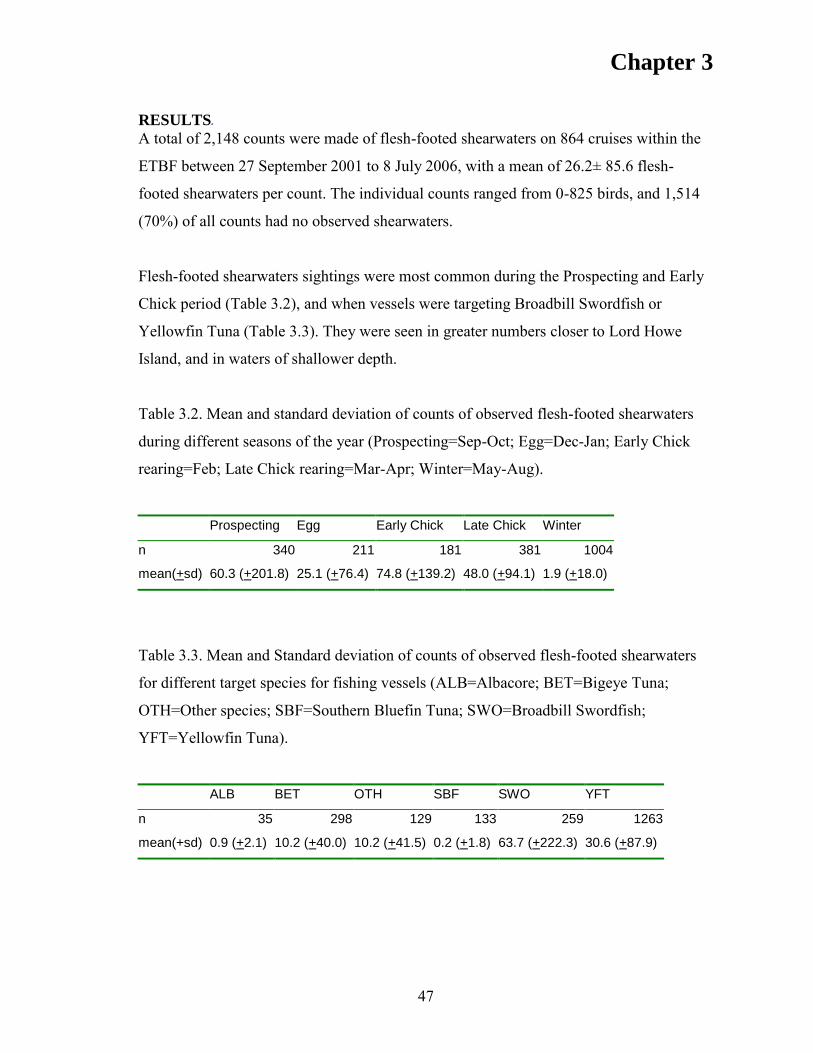
Chapter 3

47

RESULTS. A total of 2,148 counts were made of flesh-footed shearwaters on 864 cruises within the

ETBF between 27 September 2001 to 8 July 2006, with a mean of 26.2± 85.6 flesh-

footed shearwaters per count. The individual counts ranged from 0-825 birds, and 1,514

(70%) of all counts had no observed shearwaters.

Flesh-footed shearwaters sightings were most common during the Prospecting and Early

Chick period (Table 3.2), and when vessels were targeting Broadbill Swordfish or

Yellowfin Tuna (Table 3.3). They were seen in greater numbers closer to Lord Howe

Island, and in waters of shallower depth.

Table 3.2. Mean and standard deviation of counts of observed flesh-footed shearwaters

during different seasons of the year (Prospecting=Sep-Oct; Egg=Dec-Jan; Early Chick

rearing=Feb; Late Chick rearing=Mar-Apr; Winter=May-Aug).

Prospecting Egg Early Chick Late Chick Winter

n 340 211 181 381 1004

mean(+sd) 60.3 (+201.8) 25.1 (+76.4) 74.8 (+139.2) 48.0 (+94.1) 1.9 (+18.0)

Table 3.3. Mean and Standard deviation of counts of observed flesh-footed shearwaters

for different target species for fishing vessels (ALB=Albacore; BET=Bigeye Tuna;

OTH=Other species; SBF=Southern Bluefin Tuna; SWO=Broadbill Swordfish;

YFT=Yellowfin Tuna).

ALB BET OTH SBF SWO YFT

n 35 298 129 133 259 1263

mean(+sd) 0.9 (+2.1) 10.2 (+40.0) 10.2 (+41.5) 0.2 (+1.8) 63.7 (+222.3) 30.6 (+87.9)

Chapter 3

48

Modelling shearwater counts.

For the first step of the 2-step bootstrap, five variables (Distance, Breed, Wind, Altimetry

and ChlA) occurred in at least 20% of the count models, while six variables (Distance,

Breed, ChlA, Altimetry, AltAnom, and Bathy) occurred in at least 20% of the zero-

inflation models (Table 3.4). All of these variables occurred in at least one of the best

models developed in the second step of the process, and so were used in the final model

(Table 3.5). Coefficients for variables used in the final model only changed slightly

between models (Table 3.5). Time of year, Distance, ChlA and Sea Height occurred in the

zero inflated and the count model, AltAnom and Bathy occurred in the zero inflation

model and Wind occurred in the Count model. Flesh-footed shearwaters were

significantly more abundant around fishing boats in Early Chick, closer to Lord Howe

Island, at lower wind speeds, with high ChlA concentrations, with decreasing sea depth,

decreasing Sea Height and with increasing Sea Height Anomaly (Table 3.5).

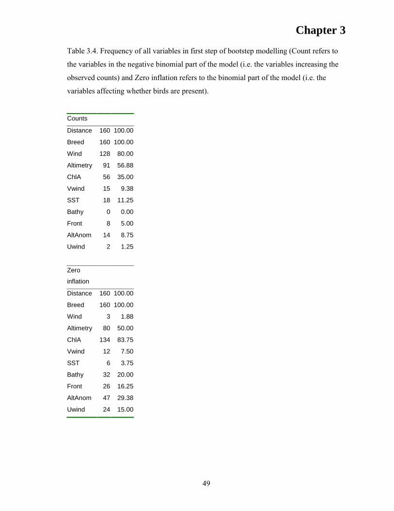
Chapter 3

49

Table 3.4. Frequency of all variables in first step of bootstep modelling (Count refers to

the variables in the negative binomial part of the model (i.e. the variables increasing the

observed counts) and Zero inflation refers to the binomial part of the model (i.e. the

variables affecting whether birds are present).

Counts

Distance 160 100.00

Breed 160 100.00

Wind 128 80.00

Altimetry 91 56.88

ChlA 56 35.00

Vwind 15 9.38

SST 18 11.25

Bathy 0 0.00

Front 8 5.00

AltAnom 14 8.75

Uwind 2 1.25

Zero

inflation

Distance 160 100.00

Breed 160 100.00

Wind 3 1.88

Altimetry 80 50.00

ChlA 134 83.75

Vwind 12 7.50

SST 6 3.75

Bathy 32 20.00

Front 26 16.25

AltAnom 47 29.38

Uwind 24 15.00

Chapter 3

50

Model validation

When the final model was used to compare predicted shearwater counts for the data set

with observer counts (Fig 3.1), there was a correlation coefficient of 0.58 (an adjusted R-

squared value of 0.33). The predicted model showed a large proportion of the data being

a zero, reflecting the pattern in the observed data (Fig. 3.1). The predicted counts were

also similar to the observed counts at lower values, but at higher observed counts, the

predicted counts tend to be underestimated (Fig. 3.1). In addition, there were less zero

counts in the predicted data than in the observed data, making thus, the observed data

over dispersed relative to the predicted data.

The season that showed the greatest difference between observed and predicted counts

was the Prospecting period, while Winter had the least. Areas with the greatest mean

deviation were around Lord Howe Island, and between Lord Howe Island and the

mainland of Australia. Most of the larger counts (>200 flesh-footed shearwaters) were

near mainland Australia between 30oS-33oS in 2001 and 2002.

Chapter 3

51

Table 3.5. Most frequently occurring models in second step of bootstrap averaging

approach. Ten chosen models were the most common 142 of 250 models. N is number of

times model occurred; Percent is percent of 142. Coefficients in Count model relate to

counts (i.e. positive coefficient indicates increasing count); coefficients in Zero inflation

model indicate proportion of zero counts (i.e. positive coefficient indicates increasing

proportion of zero counts). Mean and standard deviation (sd) calculated using methods

from Buckland et al. 1997 and Buchholz et al. 2007.

Model M15 M17 M11 M26 M3 M16 M22 M6 M12 M5 mean sd

Count Eggs -0.97 -1.00 -0.97 -0.95 -0.89 -0.97 -0.91 -0.97 -0.98 -0.90 -0.96 0.31

Late Chick -0.59 -0.61 -0.57 -0.63 -0.56 -0.59 -0.58 -0.64 -0.60 -0.52 -0.59 0.25

Prospecting -0.53 -0.54 -0.53 -0.58 -0.45 -0.53 -0.46 -0.55 -0.51 -0.40 -0.52 0.29

Winter -2.07 -2.06 -2.04 -2.09 -1.83 -2.04 -1.84 -2.09 -2.06 -1.80 -2.01 0.36

Distance 0.00 0.00 0.00 0.00 0.00 0.00 0.00 0.00 0.00 0.00 0.00 0.00

Wind -0.28 -0.27 -0.28 -0.27 -0.24 -0.27 -0.24 -0.27 -0.28 -0.23 -0.27 0.11

Alt -3.18 -3.21 -3.01 -3.13 -3.28 -2.97 -3.10 -2.50 1.83

ChlA 0.97 1.06 1.08 0.99 0.29 0.56

Intercept 8.45 8.31 8.42 8.20 7.80 8.37 7.73 8.03 8.50 7.96 8.25 0.89

Zero

inflation Eggs 0.98 0.94 1.11 1.02 1.04 1.04 1.10 0.98 0.93 1.02 1.01 0.45

Late Chick 0.60 0.61 0.63 0.64 0.65 0.65 0.65 0.62 0.58 0.66 0.62 0.37

Prospecting 1.84 1.90 2.00 1.87 1.87 1.83 2.03 1.93 1.72 1.88 1.88 0.39

Winter 3.84 3.82 4.00 3.86 3.87 3.85 4.04 3.83 3.70 3.90 3.87 0.39

Distance 0.00 0.00 0.00 0.01 0.00 0.01 0.00 0.00 0.00 0.01 0.00 0.00

ChlA -2.67 -2.59 -2.40 -2.57 -2.72 -2.28 -2.41 -2.62 -2.50 -2.29 -2.55 1.30

Alt 3.15 3.92 3.28 4.20 1.05 1.80

AltAnom -2.07 -1.11 -2.06 -0.32 0.68

Bathy -0.03 -0.03 -0.01 0.01

Intercept -4.15 -4.88 -4.43 -4.24 -4.18 -4.31 -4.47 -4.83 -4.05 -4.43 -4.38 0.72

N 40 22 14 11 11 10 10 8 8 8

Percent 28.2 15.5 9.9 7.7 7.7 7 7 5.6 5.6 5.6

AIC 3299 3305 3305 3301 3301 3303 3302 3296 3304 3309

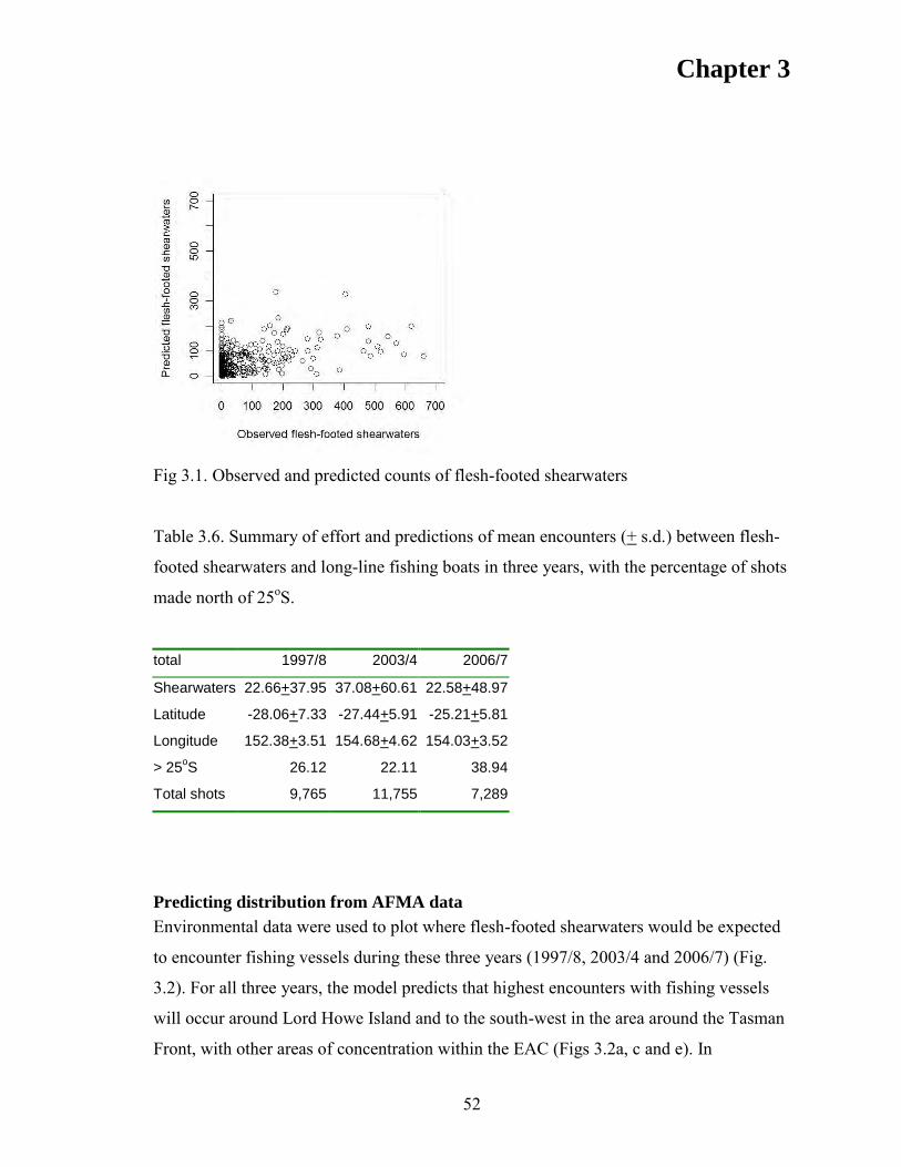
Chapter 3

52

Fig 3.1. Observed and predicted counts of flesh-footed shearwaters

Table 3.6. Summary of effort and predictions of mean encounters (+ s.d.) between flesh-

footed shearwaters and long-line fishing boats in three years, with the percentage of shots

made north of 25oS.

total 1997/8 2003/4 2006/7

Shearwaters 22.66+37.95 37.08+60.61 22.58+48.97

Latitude -28.06+7.33 -27.44+5.91 -25.21+5.81

Longitude 152.38+3.51 154.68+4.62 154.03+3.52

> 25oS 26.12 22.11 38.94

Total shots 9,765 11,755 7,289

Predicting distribution from AFMA data

Environmental data were used to plot where flesh-footed shearwaters would be expected

to encounter fishing vessels during these three years (1997/8, 2003/4 and 2006/7) (Fig.

3.2). For all three years, the model predicts that highest encounters with fishing vessels

will occur around Lord Howe Island and to the south-west in the area around the Tasman

Front, with other areas of concentration within the EAC (Figs 3.2a, c and e). In

Chapter 3

53

comparison, the distribution of fishing effort changed greatly between years. The greatest

encounters between shearwaters and long-liners were expected in 2003/4 (Table 3.6). In

1997/1998 effort was concentrated close to the coast of Australia near the EAC and also

to the north-west of Lord Howe Island in the area of 25oS 155oE off Mooloolaba (Fig

3.2b). In comparison, in 2003/2004 there was effort concentrated between Lord Howe

Island and Australia, but also to areas to the east of Lord Howe Island (Fig 3.2d). In

2006/2007 effort was concentrated to the north of 30oS and west of 155oE (Fig 3.2f) with

39% of shots north of 25oS (Table 3.6), and relatively clear of areas of greatest

encounters with flesh-footed shearwaters (Fig 3.2e).

Chapter 3

54

a. b.

c. d.

Chapter 3

55

e. f.

Fig 3.2. Predicted overlap between flesh-footed shearwaters and ETBF fishery, and

distribution of fishing effort in the ETBF. (a) Predicted encounters of fishing vessels with

flesh-footed shearwaters during 1997/1998. (b) Distribution of fishing effort in ETBF in

1997/8 (count for each one-degree block log transformed). (c) Predicted encounters of

fishing vessels with flesh-footed shearwaters during 2003/2004. (d) Distribution of

fishing effort in ETBF in 2003/4 (count for each one-degree block log transformed). (e)

Predicted encounters of fishing vessels with flesh-footed shearwaters during 2006/2007.

(f) Distribution of fishing effort in ETBF in 2006/7 (count for each one-degree block log

transformed).

Chapter 3

56

DISCUSSION

Efforts to mitigate seabird mortality in fisheries have largely focused on technological

solutions that prevent the seabirds interacting with the hazardous features of the

operation. However, a complementary approach may be to make the vessels themselves

less available to the seabirds by having them fish in areas where seabirds are less likely to

occur. These areas of higher overlap can then be highlighted, either to reduce fishing

during high encounter periods or excluding fishing if that is needed. However, these areas

of overlap are likely to also be important for fisheries. It is therefore important if using

area closures to maximize the area closed for the foraging seabirds, but minimize the area

for the fishery. Thus it is important to have as accurate a model of the distribution of the

seabirds, hence the collection of environmental variables to characterize the important

foraging areas.

While all predators should go to areas of relatively high food availability, these areas may

not be the same for each species, as they will each perceive the environment differently,

and may have different food requirements. For example, breeding seabirds such as flesh-

footed shearwaters are central place foragers, since they are required to return to their

nest for incubation and chick feeding at regular intervals, and so are restricted to within a

certain range of their breeding site (Orians and Pearson 1979; Kacelnik 1984). Fishing

vessels operating in this fishery are also central place foragers. Fish such as tuna on the

other hand have different constraints, not being required to return at regular intervals for

nesting. Therefore, they may forage in areas of increased food other than those used by

the shearwaters (Bestley et al. 2008).

Using models as explanatory tools

The distribution of flesh-footed shearwaters was best described by the time of year, and

by the distance from Lord Howe Island. They were seen in greatest numbers in the chick-

rearing, and in the prospecting periods, and least during incubation, and especially in

winter. Numbers were also inversely proportional to the distance from Lord Howe Island,

Chapter 3

57

with no birds observed more than 1000 km away. These are broadly the expected results

of the seasonal distribution of a migratory central-place forager.

In addition to the broader determinants of distribution, a number of environmental and

oceanographic variables were also important in the models. Flesh-footed shearwaters

were more commonly encountered by fishing vessels around the shelf edges or sea

mounts, rather than the open ocean. This is similar to at sea observation of the

distribution of the flesh-footed shearwaters in the Tasman Sea (Reid et al. 2002). They

were also seen in greater numbers in water with higher chlorophyll A concentration

(suggesting areas of higher productivity). Areas with lower sea height and sea height

anomaly were also important. These features suggest meso-scale cold-core eddy features,

and these and the fronts at their edges have been highlighted in previous studies of

seabird distribution (e.g. Schneider 1982, Hunt and Schneider 1987, Skov and Durinck

2000). Wind strength was negatively correlated with the numbers of shearwaters

observed. This may have indicated that the shearwaters were most active at lower wind

speeds, or alternatively, that they were more difficult to observe at high wind speeds.

These ocean characteristics are known to influence the distribution of other seabirds.

Grey-headed albatross‟ from Marion Island concentrated at the edge of both warm and

cold eddies associated with the Agulhas Current (Nel et al. 2001). Yellow-nosed

albatross‟ foraged in the Agulhas return current, concentrating in areas of increased

chlorophyll-A concentrations and in areas of sea height anomalies that indicated

productive cyclonic eddies (Pinaud and Weimerskirch 2005). Similar eddy structures are

present in the Tasman Sea in the EAC and the TF. The fronts at the edge of eddies have

been shown to be highly productive areas with increased prey (Pinaud and Weimerskirch

2005). While they are dynamic structures, and so are not going to remain in a place that

shearwaters may return to each year, they are likely to be in approximately similar

positions so that the shearwaters can move to a known region at least at larger scales.

This will have the effect of reducing the area that may need to be visited to locate food.

Chapter 3

58

The data used in our study were collected by fisheries observers, and has a number of

inherent problems, such as the attraction of fishing vessels to the birds (especially once

the first bird has arrived), and the tendency of birds to remain with a vessel once they

have located it. The quality of the data collected can be criticized due to it coming from

“non-experts”. Nevertheless it has been suggested that if you take enough non-experts

and add up their answers you will come up with the right answer by average.

Alternatively, to test the accuracy of the data, there may be a number of other methods.

Multiple observers could be used (Spear et al. 2004), however there is usually difficulty

in getting a single fisheries observer on a vessel, so opportunities for getting two on

would be rare. Taking results from several vessels operating repeatedly may be used,

however if they are close in time and space they are unlikely to be acting independently

as far as seabirds are concerned and hence are unlikely to help in improving accuracy.

Otherwise, using a modelling approach, such as adopted here, and judging if the result

appears reasonable, while recognizing the limitations of the data is the most useful

approach. Because of this, our data should be considered as encounters between the

seabirds and fishing vessels rather than being of their “normal” distribution (though, these

may be the same).

Using models as predictive tools

Models can be used for two purposes: explanatory, and predictive. Explanatory models

look to highlight the variables most associated with the observed data. Predictive models

take these relationships and attempt to use the variables to predict patterns of encounter.

Data collected by fisheries observers were useful for improving our understanding of the

distribution of flesh-footed shearwaters and in particular their encounters with long-line

fisheries. This suggests the use of observer data from fishing vessels may be appropriate

for predictive use, if the appropriate questions are being asked of it. In this case, the data

were used to model where encounters occur, rather than making an overall estimate of the

total distribution of the shearwaters. Data collected by fisheries observers is likely to be

the main source for observations of seabirds at sea in many situations. Studies of the

distribution of seabirds using at-sea observations generally exclude counts from around

commercial fishing vessels (Camphuysen et al. 2004) as this is thought to bias the results,

Chapter 3

59

causing estimates of the distribution and abundance are likely to be overestimated

(Hyrenbach 2001). However, several studies have shown that many seabirds derive a

great deal of food from around fishing vessels (e.g. Thompson and Riddy 1995; Oro et al.

1995). While the fisheries collected data may be biased in relation to at-sea observation

data, the underlying distribution of the seabirds is the same for both methods. Thus both

methods could be used for understanding this underlying distribution, though it may be

necessary to model them separately.

The model was used to predict areas with the greatest number of encounters with

fisheries in three years. By-catch of flesh-footed shearwaters is positively correlated with

the numbers present around long-liners (Lawrence et al. 2006). The years were chosen to

represent typical variation in fishing effort between years. While, on the scale of the

model, the major area of predicted interaction remained similar, the area that was actually

used by the fishery did vary considerably. Thus in 2003/2004 when the fishery was

targeting yellowfin more seriously, there was a great deal of effort into the areas that the

encounters were predicted to be greatest. Seabird by-catch rates were high in that period

(Trebilco et al. 2010). In 2006/2007 when the fishery was largely targeting albacore, most

effort was well to the north of that where encounters with the shearwaters was greatest,

and by-catch rates were relatively low (Trebilco et al. 2010). In 1997/1998 most effort

was concentrated within the EAC close to the east coast of Australia, and east of

Mooloolaba. There was relatively little effort to the south-west of Lord Howe Island in

the area of highest predicted encounters. This may suggest that mortality would have

been low for that year, though no data exists on seabird by-catch.

Broadly, the model predicted that the shearwaters will be foraging in similar areas from

year to year, with differences due to spatio-temporal differences in conditions. The area

with the highest predicted chance of encounters between fisheries and the shearwaters to

the south-west of Lord Howe Island was the area with the greatest observed mortality

over the period 1998-2004 (Baker and Wise 2005; Lawrence et al. 2006). The three years

of fishing data had major shifts in the areas being used, depending on which species were

being targeted. In recent years, fishing effort in the ETBF has changed to be targeting

Chapter 3

60

Albacore Tuna to the north of Lord Howe Island (Fig 3.2f; Baker pers. comm.). There has

been a dramatic decrease in the mortality of flesh-footed shearwaters over this time

(Baker pers. comm.). This observation validates the aims adopted in this study of

highlighting areas of increased overlap between seabirds and fisheries.

The use of area closure appears to be a viable means to reduce the mortality of seabirds

that do not prove amenable to more standard methods of mitigation. This can be seen as

analogous to the method of using Marine Protected Areas for the protection of vulnerable

fish species (Pauly et al. 2002; Hilborn et al. 2004). However, where generally in

fisheries MPA‟s are used to close specific areas, this has been argued to be of limited use

in the case of highly mobile species (Hilborn et al. 2004). Area closures were recently

adopted to protect sea turtles in Hawaii in the longline fishery for Broadbill Swordfish

(Curtis and Hicks 2000). However this involved closing a very large area from fishing.

Having greater knowledge of the requirements of more mobile species (such as their

relationships with oceanographic features) may make it possible to develop temporary

area closures. Fishers may be willing to voluntarily forgo fishing in areas that are likely

to have high by-catch if these areas can regularly be identified, and are not the only areas

they have available, especially if this avoids situations of having their fishery closed

down.

This study shows that a model with relatively simple inputs can greatly assist in our

understanding of the distribution of seabirds, and their potential foraging areas and,

importantly, where threats such as fisheries interactions are most likely to occur. This

model was developed with the aim of identifying areas where most interactions occurred,

and hence where mortalities would be likely to be highest, with the view of using it as a

dynamic, rather than static, approach to short-term area closures. These areas would be

identified from the use of a model such as this one, in particular using the explanatory

variables within the model that are variable over shorter periods (the oceanographic and

environmental variables). Further improvement could be made by identifying the rates of

change of the explanatory variables. Thus the variables on seasonal timing and position

never change, the oceanographic variables such as ocean colour and sea height potentially

Chapter 3

61

would change over periods of days and weeks, while environmental variables such as

wind speed and direction would change over periods of hours or days. The more rapidly

variables change, the less useful they are for making forward predictions, due to their

being out of date more rapidly.

CONCLUSIONS

Data collected by fisheries observers were used to model areas of interactions between

seabirds and fisheries in the ETBF. The model developed highlighted areas to the south-

west of Lord Howe Island as having increased interactions. In one of three years when

the fishery concentrated in this area there were high observed seabird mortalities, while in

another year when it concentrated in other areas, there were low observed mortalities.

This work shows the potential of area closures for the reduction of seabird mortality for

species that prove intractable to standard seabird mitigation techniques.

Chapter 3

62

ACKNOWLEDGMENTS





http://www.cdc.noaa.gov/. This study was supported by a joint CSIRO-UTas QMS joint

scholarship.

Chapter 4

63

4. Extracting information from incidental observation

data: using an arrivals-departures multi-component

model to quantify small scale habitat use in a marine

predator, the flesh-footed shearwater.

Tim Reid1,2, Mark Hindell1, Mark Bravington2 and Chris Wilcox2.


Sandy Bay, Tasmania, 7005, Australia

2Wealth from Oceans National Flagship, CSIRO Marine and Atmospheric Research,


Chapter 4

64

ABSTRACT

Collecting data for distribution or foraging information is often difficult, especially for

marine species. Obtaining designed survey data is especially rare. There is however, a

greater amount of incidental observations. These incidental data have difficulties with

biases induced due to their collection methods; for example vessel attraction effects and

autocorrelation. Statistical models that represent the processes underlying the

observations can provide a mechanism to accommodate these complexities, allowing

these other sources of data to be made available. An arrivals/departures multi-component

model has been used to examine attendance by a marine predator (the flesh-footed

shearwater) at long-line fishing vessels operating in waters of the Tasman Sea. Flesh-

footed shearwaters were predominantly attending fishing vessels while they were

operating in areas that were likely to have increased productivity, as demonstrated by

oceanographic conditions suggesting eddies and the edges of bathymetric features.

Attendance was also affected by energetic issues, as shown by their leaving vessels if

they moved over greater distances between operations, or moved further from Lord Howe

Island, the putative breeding area of the birds being observed. The results suggested that

shearwaters were more likely to attend fishing vessels in areas the shearwaters were

already likely to be feeding in, rather than the vessels acting as attractants to the areas.

This suggests vessel attendance is likely to be a local effect, and so potentially, having

vessels avoid these areas could be used by management to reduce vessel attendance by

shearwaters, and hence reduce by-catch in this fishery. The statistical technique used here

allow a better reflection of the counts than more conventional GLMs, providing better

insights on the behaviour of flesh-footed shearwaters at smaller scales than was

previously possible.

Keywords: Flesh-footed shearwater, Lord Howe Island, maximum likelihood, fishing,

long-line, by-catch

Chapter 4

65

INTRODUCTION

Predicting the distributions of species is a difficult task due to the twin challenges of

complex environmental interactions and the paucity of data. This is particularly true for

pelagic species, as they live far out to sea and thus are rarely observed. However,

understanding their distributions and the factors driving them is essential for

understanding their ecology, and is an essential component of predicting the impacts of

threats such as climate change, habitat distribution, and over-harvest by fisheries. Many

species of seabirds, especially of the family Procellariiformes, are susceptible to the

effects of fisheries, climate change and habitat destruction (Croxall and Gales 1998).

Fisheries in particular, have been linked to population declines in a number of species.

Quantifying the foraging distribution of seabirds in order to identify areas that they are

likely to interact with fisheries is an important component of managing these issues by

identifying areas of threats (Chapter 3; Pichegru et al. 2009). Further to this, adding

information from environmental drivers of these distributions will further define them at

smaller and more targeted scales. With this it may be possible to predict how future

encounters may change with changes in fisheries or climate.

There are a number of techniques that quantify the at-sea distribution of seabirds.

Advances in telemetry are increasing our ability to understand where individual birds go

(Prince et al. 1992; Shaffer et al. 2006). However, examining this has inherent biases;

generally only breeding birds are studied, and only a small number of individuals are

tracked. Alternatively, there are a great deal of data collected by observations from ships.

Ship-board observations have the advantage of having data from a great number of birds,

which is often accompanied by data on characteristics of the observation platform and the

local environment. This can include information on oceanographic variables as well as

fisheries related data such as target and non-target catch data.

There is also a range of methods that have been developed for analysing transect counts

at sea (Tasker et al. 1984, Spear et al. 2004). These methods use standardized designs

such as transect counts to minimise the effect of the observation platform. Hence they are

typically only applicable on scientific cruises or non-fisheries related shipping, as

Chapter 4

66

operations of fisheries vessels do not follow standardized protocols, and often involve

activities that attract birds making local densities higher than they otherwise would be.

Concerns about fisheries impacts upon seabirds have led to the collection of a great deal

of data from fishing boats, but these are rarely used for analyzing distribution as they do

not fit into the criteria of the standardized methods (Melvin et al 2006, Otley et al. 2007,

Chapter 3). Where fishery-based data have been used, analyses have concentrated on

broad questions of distribution and the area that the birds are observed in, without looking

at finer scale details or the oceanographic characteristics of these areas. Developing

methods that can account for these problems with fishery-based data should allow

description of seabirds‟ attendance behaviour around fishing vessels. The use of

information on the conditions that lead to seabirds attending vessels may allow

examination of these finer scales.

There are two major problems with using data from fisheries observations. The first is

that the counts are correlated since birds may follow a boat for multiple days and hence

the successive counts are not independent measures of local density. The second problem

is that fisheries involve activities that may attract (e.g. due to disposal of fish wastes from

fish processing) or repel birds (e.g. due to the presence of larger birds). Thus while the

numbers of birds attending a vessel is likely to be proportional to the local density, it is

not equivalent to it. This has been dealt with by previously either using boot-strapping

(Chapter 3), or attempting to limit counts to those birds that have newly joined the vessel

(Tasker et al. 1984, Spear et al. 2004). Boot-strapping utilises only some of the data and

so there is a loss of information and statistical power (Chapter 3). Limiting counts to only

newly joining birds is subjective, as the birds rarely have individual marks that

unambiguously distinguish them.

Given some reasonable assumptions about the underlying process, it is possible to

develop a statistical model that can accommodate these two issues. If we assume that

bird counts are correlated in a constant fashion, we can model the underlying correlation.

If we further assume that the attractiveness of the fishing vessel is either constant, or is

predictable from co-variates, then we can use the vessel as a measure of relative density.

Chapter 4

67

This would then mean that changes in the background density of birds due to habitat

quality are reflected in changes in the abundance of birds around the vessel. Thus, it

seems possible that more birds will attend a vessel while it is fishing in “good” habitat

but that they will leave when the vessel moves to “bad” habitat. From information on

the change in habitat between counts it may be possible to examine small scale aspects

of the distribution, rather than the larger scale used in previous studies. This allows

information about oceanographic and energetic effects to be analysed. These questions

cannot be answered using standard methods of analysing count data from fishing vessels.

Here a new approach to fisheries observed data has been developed using a multi-

component model, which models the birds attending a vessel by explicitly modelling the

arrivals and departures of individual birds between observations. This model was tested

using simulated data, and then applied to data on attendance by flesh-footed shearwaters

Puffinus carneipes around long-line fishing vessels in the Eastern Tuna and Billfish

Fishery (ETBF) off the east coast of Australia. Based on analysis of data from the ETBF,

the environmental and operational factors driving the spatial distribution of the

shearwaters were determined. Finally this information was used to identify areas where

encounters are predicted to be high, which is important information for management as

flesh-footed shearwaters have been shown to be threatened by mortality in this fishery

(Baker and Wise 2005).

Chapter 4

68

METHODS

Data sources

The Australian Fisheries Management Authority (AFMA) requires observers on long-line

vessels operating in Australian waters. The observers provide approximately 3%

coverage of the total fishery (Lawrence et al. 2006). In addition to collecting data on

fisheries catch and by-catch (including seabirds), observers record the number of seabirds

observed within 500 m of the vessel for a 2-3 minute period during line setting. Vessels

also record their fishing position and their daily catch, and this data is supplied to AFMA.

This data was described in more detail in Chapter 3.

In order to collect extra data for models in this paper, observers were asked to follow a

single shearwater for a period of a minute, and record whether it remained attending the

vessel, or if it departed. Departing was defined as either the bird landing on the water to

rest, or flying away to the sides or behind the vessel. Thus departure is a Bernoulli

process, with a single bird having some probability of leaving in a one minute period (or

staying as there are only two possible outcomes). Observers were also asked to record a

number of other variables, including environmental conditions and the numbers of

seabirds present at the start and finish of the counts.

Environmental parameters were obtained from a number of sources using the SDODE

software (Table 4.1) (Hobday et al. 2006). Bathymetric data (Bathy) were obtained from

2-minute Gridded Global Relief Data from the U.S. Department of Commerce, National

Oceanic and Atmospheric Administration, National Geophysical Data Center, 2006

(http://www.ngdc.noaa.gov/mgg/fliers/06mgg01.html). Sea Surface temperature (SST)

was a CSIRO 6 day composite, with accuracy to 0.036x0.042o. Sea Surface Height

(Altimetry) was MSLA, derived from the satellites TOPEX/POSEIDON and ERS-1.

Wind speed (Wind) was monthly data from using NCEP Reanalysis data provided by the

NOAA-CIRES Climate Diagnostics Center, Boulder, Colorado, USA, from their Web

site at http://www.cdc.noaa.gov/. Chlorophyll A data (ChlA) was obtained every 7.7 days

at 0.0833x0.0833o from Seawifs (http://seawifs.gsfc.nasa.gov/SEAWIFS). Frontal


http://www.cdc.noaa.gov/


Chapter 4

69

density (Front) was obtained every 7.94 days with 0.25x0.25o accuracy from CSIRO (J.

Hartog and A. Hobday unpublished). Distance (Distance) was calculated as the great

circle distance of a sighting from Lord Howe Island. Time of year (Breed) was divided

into parts of the breeding season of flesh-footed shearwaters. Changes in variables were

calculated as the value for the previous count subtracted from the current count. The

number of fish caught in the previous shot was calculated from fisheries logbook records.

Table 4.1. Co-variates used in fitting of environmental effects on arrivals and departures

of flesh-footed shearwaters behind longline fishing vessels in the ETBF.

Variable Name Description Range

Distance Km from Lord Howe Island 69-2289

Altimetry Mean sea height (m). -0.07-0.16

Bathy Depth (m). -2- -5236

ChlA Ocean productivity (mg m-3). 0.05-0.55

Front Concentration of oceanographic

fronts

0-3.59

SST oC 14.54-29.32

Wind Wind speed (m s-1) 4.35-9.46

Fish Number of fish caught on

previous shot

0-185

DistToPrev Distance to previous shot (km) 0-1111

Latitude Latitude (oS) 38.87-14.60

ChangeInBathy Change in bathymetry since last

shot (m)

-3365-3255

ChangeInSST Change in SST since last shot (oC) -8.21-11.99

ChangeInAltimetry Change in Sea Height since last

shot

-0.17-0.14

ChangeInChlA Change in Ocean productivity

since last shot

-0.37-0.30

Chapter 4

70

Model development

Changes in seabird abundance at a given vessel between successive observations were

modelled as a mechanism for comparing the relative quality of different environmental

conditions. It was assumed that the vessel, subject to covariates, has a constant

attractiveness to birds, so that changes in the density of seabirds between fishing

operations are due to changes in habitat quality between the sites. We modelled the

changes in these counts using a multi-component model. Our approach considered three

levels of uncertainty: process uncertainty, parameter uncertainty and measurement

uncertainty.

In order to model the process, it was assumed that birds depart from the vessel after a

count, and then subsequently new birds arrive prior to the next count. While this is

somewhat artificial, it enables the intervening number of birds to be treated as a hidden

variable that has a finite number of states, ranging from the number on the first count to

zero. This is an essential feature, as it allows the integration of the likelihood over this

hidden state, and thus we can estimate the likelihood of the observations given a set of

parameters (Fig. 4.1).

Departures, D, were modelled for a given observation as an integer between the number

observed on the first count, Ci , and zero, using a binomial distribution to describe the

process.

Pr 1

logit

i ii

i

i C ddi

i

d

CD d p p

d

p X

. Equation 1

where i is the observation number, d is the probability of departure, p is the leaving rate

per minute, is the coefficients of the departures variables, and X are the environmental

Chapter 4

71

variables that effect departure. The difference between this random variable and the first

count, Ci - Di, is a hidden variable that is not observed.

Fig 4.1. Simplified diagram of process involved between successive counts, where N2 is

the current count, N1 is the observed number of birds during a previous count, and Nu is

the number present at some unobserved time in between.

Arrivals of new birds at the vessel join this, yielding the count at the second observation.

We model these arrivals as a Poisson process, yielding integers bounded by zero and

infinity

Pr!

ln

aeA aa

Y

Equation 2

where A is the number of arrivals, Y are the environmental variables that effect arrivals, a

is the probability of arrivals, α is the coefficients on the arrivals variables, and φ is the

arrival rate.

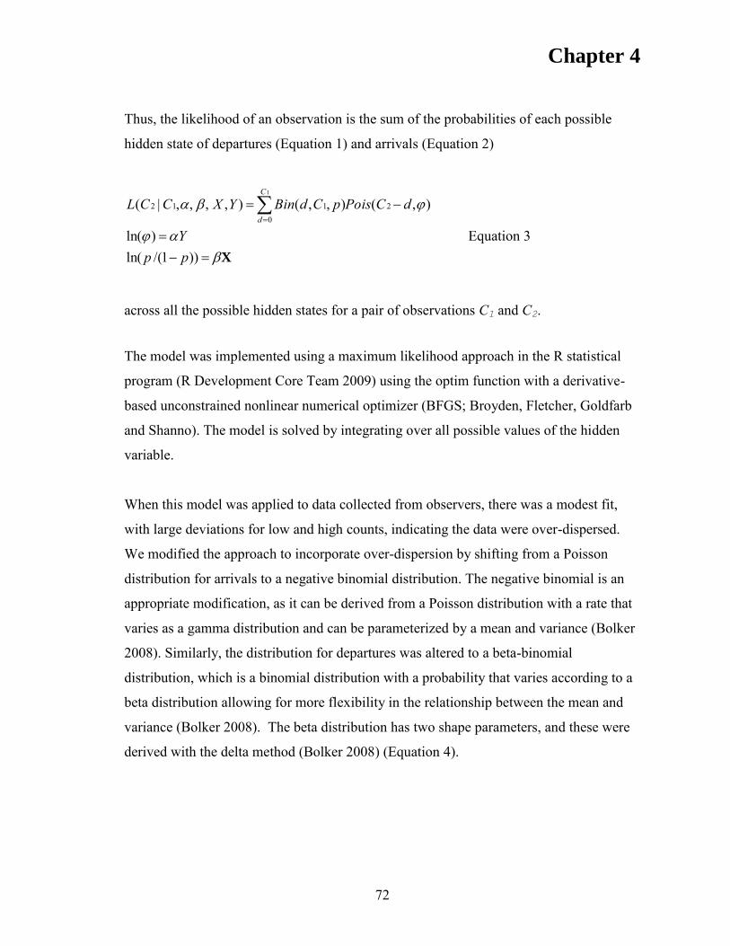
Chapter 4

72

Thus, the likelihood of an observation is the sum of the probabilities of each possible

hidden state of departures (Equation 1) and arrivals (Equation 2)

X

))1/(ln()ln(

),(),,(),,|( 20

112

1

ppY

dCPoispCdBinYXCCLC

d

Equation 3

across all the possible hidden states for a pair of observations C1 and C2.

The model was implemented using a maximum likelihood approach in the R statistical

program (R Development Core Team 2009) using the optim function with a derivative-

based unconstrained nonlinear numerical optimizer (BFGS; Broyden, Fletcher, Goldfarb

and Shanno). The model is solved by integrating over all possible values of the hidden

variable.

When this model was applied to data collected from observers, there was a modest fit,

with large deviations for low and high counts, indicating the data were over-dispersed.

We modified the approach to incorporate over-dispersion by shifting from a Poisson

distribution for arrivals to a negative binomial distribution. The negative binomial is an

appropriate modification, as it can be derived from a Poisson distribution with a rate that

varies as a gamma distribution and can be parameterized by a mean and variance (Bolker

2008). Similarly, the distribution for departures was altered to a beta-binomial

distribution, which is a binomial distribution with a probability that varies according to a

beta distribution allowing for more flexibility in the relationship between the mean and

variance (Bolker 2008). The beta distribution has two shape parameters, and these were

derived with the delta method (Bolker 2008) (Equation 4).

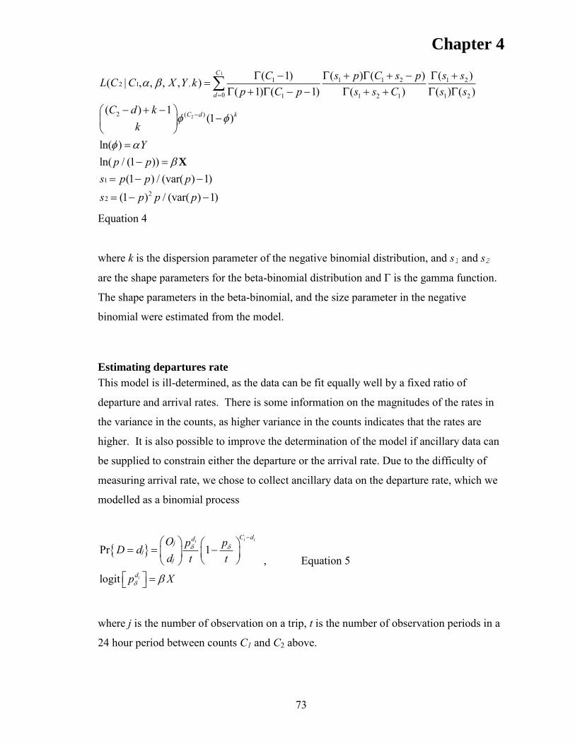
Chapter 4

73

1

2

1 1 1 2 1 22 1 ,0 1 1 2 1 1 2

2 ( )

1

22

( 1) ( ) ( ) ( )( | , , )( 1) ( 1) ( ) ( ) ( )

( ) 1(1 )

ln( )ln( / (1 ))

(1 ) / (var( ) 1)(1 ) / (var( ) 1)

C

d

C d k

C s p C s p s sL C C X Y kp C p s s C s s

C d kkY

p ps p p ps p p p

X

Equation 4

where k is the dispersion parameter of the negative binomial distribution, and s1 and s2

are the shape parameters for the beta-binomial distribution and Γ is the gamma function.

The shape parameters in the beta-binomial, and the size parameter in the negative

binomial were estimated from the model.

Estimating departures rate

This model is ill-determined, as the data can be fit equally well by a fixed ratio of

departure and arrival rates. There is some information on the magnitudes of the rates in

the variance in the counts, as higher variance in the counts indicates that the rates are

higher. It is also possible to improve the determination of the model if ancillary data can

be supplied to constrain either the departure or the arrival rate. Due to the difficulty of

measuring arrival rate, we chose to collect ancillary data on the departure rate, which we

modelled as a binomial process

Pr 1

logit

i ii

i

C ddjj

j

d

O p pD dd t t

p X

, Equation 5

where j is the number of observation on a trip, t is the number of observation periods in a

24 hour period between counts C1 and C2 above.

Chapter 4

74

Model validation

The ability of this model to recover known parameters was tested by simulating data and

then fitting the model to that data to see if the parameters could be accurately estimated.

Initially, 1,000 first counts were simulated using a Poisson distribution. For each of these

first counts, a second count was generated by having the birds of the initial count

randomly leave following a binomial distribution, and other birds arriving following a

Poisson distribution. The second count was therefore the first count minus the departures,

plus the arrivals. These arrivals and departures were each effected by normally distributed

co-variates multiplied by co-efficient values. These data were then run through the model

that had been developed to test whether it would successfully retrieve the parameters in

the data.

To test the effect of model complexity on fit, the model was run using from one to five

generated explanatory variables. In order to test the performance of the model for a range

of values, the coefficient for one of the random covariates was varied by one sequentially

between –5 and 5, and the value of the parameter used to generate the model, and the

estimate derived from the maximum likelihood were recorded. The correlation between

these was then calculated and evaluated for each of one to five generated variables. While

the parameter for a single generated variable was varied, all other variables were held

constant, and the estimates of these parameters, and the residuals of the estimates were

recorded.

The ability of the model to recover true parameters for each of the components, arrivals

or departures, and for both together was tested.

To test the effectiveness of the model in comparison to other methods, it was tested

against a Generalised Linear Model (GLM) using a Poisson distribution with a log link

function. To do this, data were simulated in the same way to that used to test the model.

Counts at the two successive time steps were generated for 1,000 observations, using a

single normal random explanatory variable and parameter to generate count 2. This was

done for a range of parameter values, varying sequentially from –5 to 5 by one. A two

Chapter 4

75

component model was fit to the data using maximum likelihood. A standard Poisson

GLM was then fit to the data, using the independent variable (the simulated co-variate) to

describe the dependent variable (the final count). The fitted co-variate from this GLM

was then recorded for each of simulated data sets. The parameters identified from each of

the two component models and the Poisson GLMs were then plotted against the “true”

parameter, to identify which model performed better in terms of recovering the

underlying process.

Estimating departure of individuals

Individual departure data took the form of a binomial distribution. To test which variables

were most affecting departures, it was analysed with a Generalised Linear Model (GLM)

using a logistic link function using the R statistical program version 2.9.0 (R

Development Core Team 2009). To test which variables were significant, we used a

stepwise addition of variables using the step function in R. Variables were standardized

by subtracting the mean and then dividing by the standard deviation (Sokal and Rohlf

1969).

Model fitting

In order to identify which variables were having the greatest effect on the number of

shearwaters present, a forward stepwise process was used. Variables were added or

subtracted using comparisons of the AICc (Burnham and Anderson 1998). Standardized

residuals were then used to diagnose whether the distributions of the random variables

accommodated the variation observed in the process. This process was carried out for the

models developed from Equation 3 and Equation 4.

Chapter 4

76

RESULTS

Observations of flesh-footed shearwaters collected by AFMA fisheries observers were

used in the study; it was described in greater detail in Chapter 3. All data occurred off the

east coast of Australia, with sightings of flesh-footed shearwaters recorded between 15-

40oS (Fig 4.2). For analysis in this paper, 1,233 observations that were preceded by other

counts were used.

Fig 4.2. Locations of all observer counts of flesh-footed shearwaters by AFMA observers

in the ETBF. Observations are represented by a point; counts by circles (circles

proportional to the log of the number of shearwaters counted).

Model validation

The model was successful at retrieving the parameters from simulated data (Fig. 4.3).

Correlations were greater than 0.96 for up to 4 parameters, showing that the model could

retrieve the patterns in the simulated data (Fig 4.3a). In one simulation with four

parameters, there was a relatively poor correlation (0.78) when one level of one

parameter value was retrieved inaccurately (Fig 4.3a). This was a case with the varied

parameter describing the arrivals, while variables describing the arrivals were held

Chapter 4

77

constant. The poor retrieval of this value may suggest that the likelihood surface was

fairly flat, or that there were more than one minima in the surface or alternatively,

because there is randomness in the data being modelled, some fraction of the estimated

values will be poor. There was some deterioration in performance for 5 parameters,

though all correlations were greater than 0.93 (Fig 4.3a). Mostly residuals remained

close to the Fitted values, though they appeared to become greater at larger values (Fig

4.3b). In some cases where there were only parameters on one side of the model, the

estimate of the constant probability of the other side of the model became less accurate

with increasing numbers of parameters (Fig 4.3c). It was most inaccurate when the

departures were held at constant probability (and hence the parameters were describing

the arrivals) (Fig 4.3d). The coefficients that were held constant were retrieved accurately

for up to four parameters (Fig 4.3e). For five parameters there was a tendency to

overestimate the parameter on the departures (Fig 4.3f).

Chapter 4

78

a. b.

c. d.

1 2 3 4 5

0.8

00.8

50.9

00.9

51.0

0

Number of parameters

Corr

ela

tion

param on depart

param on arrive

param on both (vary on depart)

param on both (vary on arrive)

1 2 3 4 5

020

40

60

80


Resid

uals

fro

m t

he inte

rcept

param on depart

param on arrive

param on both

1 2 3 4 5

-20

020

40

60

80


Resid

uals

of

com

ponent

with n

o c

ovariate

Chapter 4

79

e. f.

Fig 4.3. Results from simulation trial of model with up to five added parameters. (a).

Correlation between the parameter that was varied, and the estimate of the parameter

from the model. Horizontal line at 1 indicates level if there was perfect correlation. Var

on arrive = parameters on arrivals; var on depart = parameters on departures; var on both

= parameters on both parts of model. (b). Residuals for fitted values from simulation

trials. (c). Residual values of the mean intercepts for different models with increasing

numbers of parameters. Var on arrive = parameters on arrivals; var on depart =

parameters on departures; var on both = parameters on both parts of model. (d). Mean

and range of residual values of mean intercepts for models with increasing numbers of

parameters. (e). Residuals of the estimated mean value of parameters held constant while

correlation was examined for one parameter. Var on arrive = parameters on arrivals; var

on depart = parameters on departures; var on both = parameters on both parts of model.

(f). Mean and range of residuals of estimated mean values of parameters held constant

while the correlation was examined for one parameter.

The performance of the model and a GLM was compared using simulated data. The

correlation of parameters derived using the model showed a strong correlation with the

simulated parameters (0.99); that between the parameters estimated from the GLM and

the simulated parameters of -0.97, hence it retrieved the parameters poorly (Fig 4.4).

1 2 3 4 5

-0.4

-0.2

0.0

0.2

0.4

0.6

0.8


Resid

uals

of

unvaried p

ara

mete

rs

param on depart

param on arrive

param on both (vary on depart)

param on both (vary on arrive)

2 3 4 5

-0.4

-0.2

0.0

0.2

0.4

0.6

0.8


Resid

uals

of

unvaried p

ara

mete

rs

Chapter 4

80

Fig 4.4. Comparison of retrieval of simulated parameters using the model (circles) and a

Generalised Linear Model with a Poisson distribution and a log link (squares).

Departure rates

Observers made 270 one minute dedicated observations of flesh-footed shearwaters

behind long-line fishing boats between 17 February 2008 and 8 July 2009. During these

observations, 20 birds left during the observation period, giving a rate of 0.074

departures.m-1 (s.d. = 4.30), giving a probability of leaving during one minute of 0.071.

Flesh-footed shearwaters were more likely to stay behind the vessel with increasing

numbers of shearwaters behind the vessel, with increasing distance from Lord Howe

Island, with decreasing numbers of petrels behind the vessel and with increasing latitude.

Latitude had the strongest effect on the number of shearwaters staying, while the number

of petrels had the least influence (Table 4.2).

Model fitting

Initially, the data were modelled using Equation 3 (with binomial departures and Poisson

arrivals). The best model using this structure was with departures affected by sea surface

height and bathymetric gradient, and arrivals were affected by the wind strength (Table

-4 -2 0 2 4

-4-2

02

46

Parameter

Estim

ate

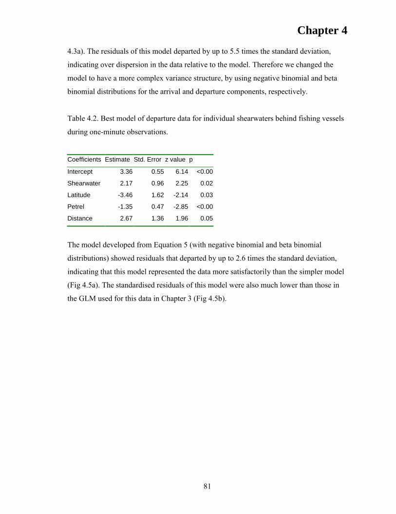
Chapter 4

81

4.3a). The residuals of this model departed by up to 5.5 times the standard deviation,

indicating over dispersion in the data relative to the model. Therefore we changed the

model to have a more complex variance structure, by using negative binomial and beta

binomial distributions for the arrival and departure components, respectively.

Table 4.2. Best model of departure data for individual shearwaters behind fishing vessels

during one-minute observations.

Coefficients Estimate Std. Error z value p

Intercept 3.36 0.55 6.14 <0.00

Shearwater 2.17 0.96 2.25 0.02

Latitude -3.46 1.62 -2.14 0.03

Petrel -1.35 0.47 -2.85 <0.00

Distance 2.67 1.36 1.96 0.05

The model developed from Equation 5 (with negative binomial and beta binomial

distributions) showed residuals that departed by up to 2.6 times the standard deviation,

indicating that this model represented the data more satisfactorily than the simpler model

(Fig 4.5a). The standardised residuals of this model were also much lower than those in

the GLM used for this data in Chapter 3 (Fig 4.5b).

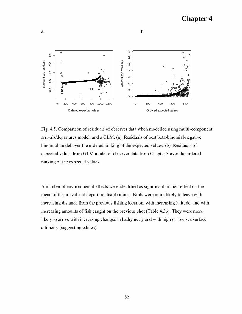
Chapter 4

82

a. b.

Fig. 4.5. Comparison of residuals of observer data when modelled using multi-component

arrivals/departures model, and a GLM. (a). Residuals of best beta-binomial/negative

binomial model over the ordered ranking of the expected values. (b). Residuals of

expected values from GLM model of observer data from Chapter 3 over the ordered

ranking of the expected values.

A number of environmental effects were identified as significant in their effect on the

mean of the arrival and departure distributions. Birds were more likely to leave with

increasing distance from the previous fishing location, with increasing latitude, and with

increasing amounts of fish caught on the previous shot (Table 4.3b). They were more

likely to arrive with increasing changes in bathymetry and with high or low sea surface

altimetry (suggesting eddies).

0 200 400 600 800 1000 1200

0.5

1.0

1.5

2.0

2.5

Ordered expected values

Sta

ndard

ised r

esid

uals

0 200 400 600 800

02

46

810

12

14

Ordered expected values

Sta

ndard

ised r

esid

uals

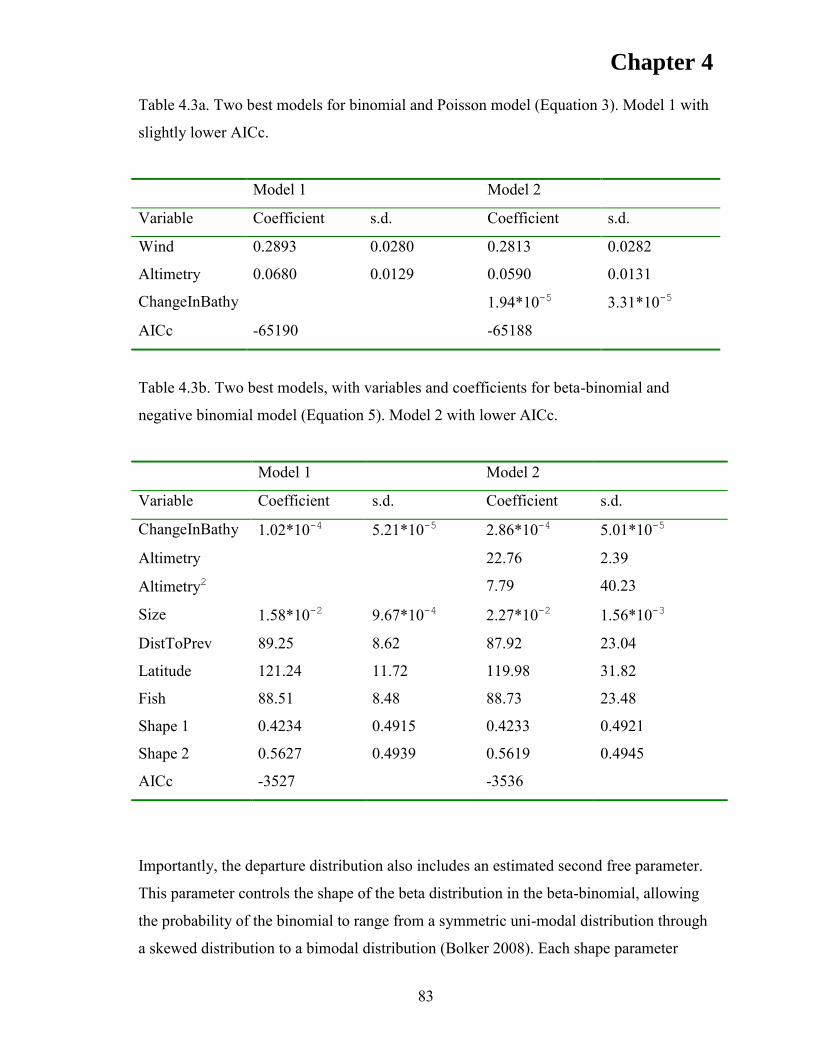
Chapter 4

83

Table 4.3a. Two best models for binomial and Poisson model (Equation 3). Model 1 with

slightly lower AICc.

Model 1 Model 2

Variable Coefficient s.d. Coefficient s.d.

Wind 0.2893 0.0280 0.2813 0.0282

Altimetry 0.0680 0.0129 0.0590 0.0131

ChangeInBathy 1.94*10-5 3.31*10-5

AICc -65190 -65188

Table 4.3b. Two best models, with variables and coefficients for beta-binomial and

negative binomial model (Equation 5). Model 2 with lower AICc.

Model 1 Model 2

Variable Coefficient s.d. Coefficient s.d.

ChangeInBathy 1.02*10-4 5.21*10-5 2.86*10-4 5.01*10-5

Altimetry 22.76 2.39

Altimetry2 7.79 40.23

Size 1.58*10-2 9.67*10-4 2.27*10-2 1.56*10-3

DistToPrev 89.25 8.62 87.92 23.04

Latitude 121.24 11.72 119.98 31.82

Fish 88.51 8.48 88.73 23.48

Shape 1 0.4234 0.4915 0.4233 0.4921

Shape 2 0.5627 0.4939 0.5619 0.4945

AICc -3527 -3536

Importantly, the departure distribution also includes an estimated second free parameter.

This parameter controls the shape of the beta distribution in the beta-binomial, allowing

the probability of the binomial to range from a symmetric uni-modal distribution through

a skewed distribution to a bimodal distribution (Bolker 2008). Each shape parameter

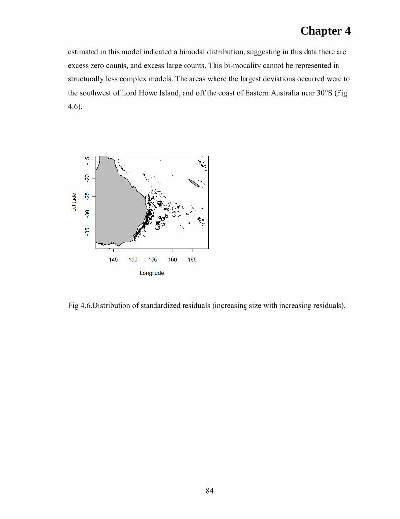
Chapter 4

84

estimated in this model indicated a bimodal distribution, suggesting in this data there are

excess zero counts, and excess large counts. This bi-modality cannot be represented in

structurally less complex models. The areas where the largest deviations occurred were to

the southwest of Lord Howe Island, and off the coast of Eastern Australia near 30oS (Fig

4.6).

Fig 4.6.Distribution of standardized residuals (increasing size with increasing residuals).

Chapter 4

85

DISCUSSION

A great deal of information about the distribution and abundance of seabirds is collected

by fisheries observers during observations of fisheries operations. These are generally

analysed at only the most basic level, indicating areas with increased numbers of birds

around fishing vessels. These data have been regarded as a biased measure of seabird

distribution and unable to be used for more complex analyses such as quantifying habitat

associations (Camphuysen et al. 2004). Nevertheless Chapter 3 showed that if carefully

chosen questions were asked, fisheries observer data could be used to usefully describe

the habitat associations of the species. Taking account of the vessel‟s changing effect

further improves this in terms of understanding relative abundance.

Many studies have shown that ecosystems operate over a range of scales (Wiens 1989,

Schneider 2001). Foraging by seabirds is an example of a process operating at multiple

scales in this fashion. At meso scales, breeding seabirds are constrained in how far they

move from colonies due to the requirement to regularly feed their chicks, thereby

determining the overall distribution of the birds. But within this larger scale, they will

also respond to smaller scale features, for example when locating areas to forage. Areas

in which they feed will be determined by local ecological processes such as up-wellings

at the edges of eddies. While they may overall have a limited area in which to feed, they

actually only use a subset of that and forage in suitable habitat. Therefore it is invaluable

to consider a range of scales. Thus raw counts of seabirds behind fishing vessels can be

used for looking at the distribution of interactions, but with relative counts it is possible

we can look at habitat selection.

Animal survey data are often derived as a series of counts that are potentially

autocorrelated. Autocorrelation may come from a number of sources, commonly in

ecology it may derive from patchy distributions, however it may also be a result of

successive counts along a spatial or temporal transect (Schneider 1990, 2001). A patchy

distribution may result in an uneven spread of some feature of an area being studied,

while spatial or temporal transects may be autocorrelated through the animal being

Chapter 4

86

studied following the studier from count to count. This is often dealt with by considering

the variance structure, or not using some of the data (Bolker 2008). In this paper a multi-

component arrivals/departures (AD) model was used to examine the second source of the

autocorrelation. The study demonstrates that application of appropriate statistical

methods applied to the complete data sets can provide new insights into the relationships

between successive counts that otherwise would be treated as noise and discarded. This

allows the study of the biology and oceanography of these successive counts to be

captured.

The AD model accurately retrieved simulated data and gave a more accurate retrieval

from simulated data than using a GLM. This is not unexpected, as the simulated data

were generated using an arrivals/departures process that was more similar to the process

used in the AD model. Evaluating the fit of the model to field data, residuals derived for

the AD model were lower than those from a single component GLM when fitted to

observer data. This is a useful validation of our model, as it is not a foregone conclusion

that the AD model would provide a better fit. In addition to giving a better fit, the AD

model is a more accurate representation of the hypothesized process that is occurring (i.e.

birds are arriving and departing). While the model is still a simplification, it allows the

introduction of such features as the bimodal shapes of departures. Simpler models, such

as single component GLMs do not allow this. At some point adding further complexity in

a model no longer adds greater fit. The bi-modal nature of the model here may suggest

that there are two processes operating (such as a factor with two states), but which the

model and data set do not have any information on that would allow the inclusion of an

extra co-variate.

The model will work for counts that follow on from previous counts; however in its

current form it cannot be used for the initial count during a cruise. This is because the

initial count will relate to a somewhat different process. For the first count, birds will join

the vessel from there being none present, and this relates to the water in between the port

the vessel leaves from, until it gets to the site of the initial count, and will need to take

into consideration all water masses that are crossed in between these positions. In

Chapter 4

87

addition, the first count will be a result of a cumulative process over a few days as vessels

often steam for some time before fishing. Nevertheless, there will be times when the

initial count could be fit into this model. Potentially this could be added by fitting the first

count with a distribution such as a Poisson or negative binomial and parameters such as

distance from port. It could then be fitted to the overall model with a joint likelihood.

However, it is unclear whether this would lead to extracting more information on habitat

associations, as this would be determined by the information content in the first counts

versus the similarity of the underlying process to the other processes being modeled.

Most previous studies using data collected by fisheries observers have addressed broad

scale, such as identifying the large scale distribution of seabirds (e.g. Otley et al. 2007;

Chapter 3). However, by using single component models these investigations confound

factors driving distributions at large and small scales. This study quantified the finer

(coarse) scale environmental features of the distribution. The models indicated five

influential factors.

Shearwaters were predicted to be more likely to leave the fishing boat with increasing

distance between shots. This may be interpreted either as indicating the birds are less

likely to stay with a vessel with increasing movements between fishing activities, which

is akin to increasing distances between patches from an optimal foraging perspective

(Charnov 1976). This is suggesting an energetic consideration for the shearwater.

Alternatively, it may indicate that with increasing distance the vessel was more likely to

have moved from an area the shearwater was feeding in to an area that the shearwater

was less likely to feed in, suggesting a habitat-related cue.

Also important was increasing latitude, with shearwaters leaving as the vessel moved

further north. This suggests that the vessel was moving into less suitable habitat the

further north it travelled.

The magnitude of the catch on the previous shot was important, with shearwaters more

likely to leave with greater catch, suggesting they had eaten sufficient food and hence left

Chapter 4

88

the vessel and returned to their colony, or alternatively, that the vessel had been operating

in a productive area (hence the large catch) but that it had moved into areas that were less

favourable to the shearwaters. Returning to the colony would be an energetic cue for the

shearwater, while the alternative would suggest the vessel had left the suitable habitat.

Shearwaters arrived behind vessels more often with increasing (and an increasing change

in) bathymetry. They were also more likely to arrive with the absolute depth being

shallower, though the addition of this variable made the model worse. The shearwaters

were therefore more likely to arrive behind vessels as the vessel moved into shallower

water, such as if it moved onto a shelf or sea mount, but at the edge of the bathymetric

feature. Shelf breaks have been demonstrated to be productive and attractive to seabirds

(Haney 1986; Alderman et al. 2010).

Shearwaters were predicted to be more likely to arrive with high or low sea surface

height. This suggests they were more likely to arrive when vessels are at eddies. Eddies

generally have up-wellings and down-wellings, and so are particularly productive, and

hence more likely to have food. Seabirds generally are thought to concentrate in these

areas naturally (Haney 1986; Pinaud and Weimerskirch 2005), suggesting that the

shearwaters are arriving behind the vessels because they are operating in areas that are

good habitat.

Overall from the models, it is apparent that the shearwaters were more likely to attend

vessels with increasingly productive areas (increased catch, eddies, shelf breaks) and with

energetic considerations (departing with increasing distance from the previous shot). The

oceanographic co-variates suggest that shearwaters were attending fishing vessels

dependent on up-wellings or down-wellings, or the edges of bathymetric features, all of

which are likely to be associated with eddy features. In the Baltic Sea, seabirds only

attended fishing vessels which were operating in conditions with high productivity, but

generally ignored vessels discharging fish when in unproductive waters (Skov and

Durinck 2001). Elsewhere, in New Zealand Westland petrels Procellaria westlandica

only foraged around fishing vessels that were operating in the areas that the petrels

Chapter 4

89

naturally feed (Freeman 1997). Attendance at fishing vessels by seabirds is therefore a

local effect, though the size of this may differ depending on the mobility of the species.

Attendance may only be initiated if the vessel is in a chosen foraging zone, but once one

seabird has commenced attendance, it may act to attract many other seabirds from an area

around due to flocking behaviour. The overdispersed residuals in the model may suggest

flocking, which can be a useful method for foragers to pass information to each other in a

patchy environment (Clark and Mangel 1984).

This study has demonstrated the utility of the AD modelling approach in analysing

fisheries observer data of succeeding counts of seabirds, but can be applied more

generally where there is a series of counts of populations but not of identifiable

individuals. Commonly, there is autocorrelation due to the carrying over of individuals in

time or space, such as for seedlings in forest quadrats or changes between locations of

spotlight surveys of mammals (e.g. Harms et al. 2001; Caley and Morley 2002). The AD

model may be particularly useful in situations where this carry over is thought to have

some ecologically meaning information. For the seabirds the counts in sequential

positions were related but changed due to the underlying oceanographic conditions. This

may be equally relevant in spotlight surveys of mammals, though perhaps less so in

seedling quadrats. Only a small amount of extra information is required due to the data

being ill-determined. But it is relatively easy to get the data on the departures, and that

sort of data is likely to be obtainable in other situations if a small amount of time is

dedicated to it.

Chapter 4

90

ACKNOWLEDGEMENTS





http://www.cdc.noaa.gov/. This study was supported by a joint CSIRO-UTas QMS joint

scholarship. Scott Foster (CSIRO) assisted with fisheries data. Jim Dell assisted with

SDODE code.

Chapter 5

91

5. The importance of recent experience and

environment in determining large scale foraging

patterns in a pelagic seabirds, the flesh-footed

shearwater.

Tim Reid1,2, Mark Hindell1, Richard Phillips3 and Chris Wilcox2.


Sandy Bay, Tasmania, 7005, Australia

2Wealth from Oceans National Flagship, CSIRO Marine and Atmospheric Research,


3British Antarctic Survey, Natural Environment Research Council, High Cross,

Madingley Road, Cambridge CB3 0ET, UK

Chapter 5

92

ABSTRACT

We hypothesized that marine predators should take advantage of previous experience in

locating foraging areas. Using experience of previous foraging areas is likely to increase

foraging efficiency and increase the effectiveness of search methods such as area-

restricted search or Lévy flights by locating the better areas initially, thereby reducing the

subsequent search effort. At a coarse scale, for each visit to an area by a flesh-footed

shearwater during the current trip, the odds of visiting the same area increased by

between 5-531%, for each visit in the previous trip the odds of returning in the current

trip increased by between 2-46% and for each visit in the second last trip, by between 4-

25%. Using the length of time spent in an area as a proportion of previous trips as a

proxy for quality of foraging in that area, we also identified a strong effect on the

probability that birds chose to visit high quality locations on future trips. At the coarse

scale, they were more likely to choose to visit an area with increasing Sea Surface Height

Anomaly, while during incubation they chose to visit areas with increasing Sea Surface

Temperature, but decreasing during chick-rearing. They were less likely to visit an area

with increasing Chorophyll-a. At the coarse scale, the use of experience was at least as

important as any of the oceanographic variables tested.

Keywords: flesh-footed shearwater, Lord Howe Island, foraging, experience, memory,

choice, Discrete Choice Model

Chapter 5

93

INTRODUCTION

Pelagic marine predators live in an environment with patchily distributed resources,

which presents challenges for them obtaining energy at sea (Weimerskirch 2007). Marine

predators using the pelagic environment are characterised by foraging over large

distances to encounter these dispersed resources (Jouventin and Weimerskirch 1990,

Prince et al. 1992; Weimerskirch et al. 1999; Hindell et al. 2003; Phillips et al. 2006).

This results in a relatively slow uptake of energy and leads to them having specialised

breeding system such as low productivity and high investment in adult survival

(Weimerskirch et al. 1987; Hindell 1991, Bradley et al. 2008). Many species, such as

seabirds or seals, produce only a single young each year, and while survival of this

offspring to breeding age is relatively low, once they reach breeding age, survival is high.

In this context one would expect animals to adopt behaviours that maximize their

encounter rate with ephemeral resource patches. Two possible mechanisms for achieving

this end are utilization of efficient search methods and use of information from

experience.

There is only limited information on the strategies they may employ to find these patchily

distributed resources (Weimerskirch et al. 2005). Physical processes such as currents and

their interactions with bathymetry are known to affect the distribution of plankton (Hunt

et al. 1996). Seabirds, marine mammals and fish have all been shown to respond to such

areas as fronts, shelf edges and up-wellings where productivity and prey are likely to be

concentrated (Hunt et al. 1996; Young et al. 2001; Call et al. 2008). Several strategies

could improve encounter rates with patchy resources; four are proposed here with

increasingly complex use of information: i) use of search algorithms; ii) use of

environmental cues; iii) previous experience of static features; and iv) previous

experience of dynamic features.

Marine predators have been suggested to use efficient search methods for locating food

resources, such as area restricted search, correlated random walks, Lévy flights and

fractal patterns (Viswanathan et al. 1996; Fauchald and Tveraa 2003; Tremblay et al.

2007). While these methods decrease search times, they do not utilize information, and as

Chapter 5

94

such are unlikely to be employed in isolation of other sources of information. The use of

environmental cues will provide better informed searches, but is only useful when the cue

is present in real time. At meso- and sub-mesoscales (<10 km), seabirds find productive

areas through smell or observing other predators (Au and Pitman 1986; Haney et al.

1992; Nevitt et al. 2008; Tew Kai et al. 2009).

Some predators return to approximately similar areas on consecutive foraging trips

(Bradshaw et al. 2004; Weimerskirch et al. 2005). This provides qualitative evidence for

the use of experience or inheriting, although it is static experience in the sense that once a

pattern is learned it does not need to change (Weimerskirch 2007; Call et al. 2008). The

most complex use of memory in foraging is dynamic memory, where areas of high

quality habitat are remembered from past experience, but the interpretation of that

information changes with time. One example would be discounting of information with

time, such that the most recent experience is given the highest weight in predicting

suitable areas in which to forage. Learning is useful if it enhances the long term fitness of

an animal through behavioural changes, such as providing flexible search strategies when

the environment shows temporal change (Eliassen et al. 2007, 2009). If variability is

spatial, but does not vary over time, it is less important to be able to learn rapidly or

forget the distant past (Mangel 1990; Eliassen et al. 2009). Learning is more useful with

increasing life span (Eliassen et al. 2007).

Many marine predators are central place foragers, and thus their use of search tactics is

constrained by the need to return to their breeding sites on a regular basis (Ashmole

1971). For seabirds there is a further restriction with differing behaviour during the

breeding season due to whether they have eggs or chicks. When incubating eggs, the

parents alternate at sea for relatively long trips. Since these foraging bouts have a fixed

length, we hypothesize that the foragers will concentrate primarily on increasing their

reserves by maximizing the net energy gain during their foraging bout. However, when

they are on chicks (especially newly hatched) the condition of the chick declines the

longer the foraging parent is away, thus we expect to the forager to maximize the rate of

energy uptake by the chick, instead of the net amount going to the forager. We expect

Chapter 5

95

that this difference will constrain the parent‟s ability to explore for new information

during chick rearing, and leading birds to prefer reliable areas they have successfully

foraged in previously. This preference would be expected to increase the importance of

experience, and should be visible in their foraging patterns.

In this study we explore the importance of experience, and its impact relative to other

environmental cues on foraging by flesh-footed shearwaters, Puffinus carneipes, nesting

on Lord Howe Island. We address four questions in relation to the foraging of flesh-

footed shearwaters: i) do they return to similar areas to those they have previously

visited; ii) how does past success in the area affect this decision; iii) are they more likely

to visit areas due to experience, or due to measured environmental variables; and iv) is

the initial position after leaving the colony chosen differently from later positions.

Chapter 5

96

METHODS

Study site and species Flesh-footed shearwaters are a medium sized shearwater that breed on a number of

islands, including Lord Howe Island in the Tasman Sea (31o30‟S 159o05‟E) (Marchant

and Higgins 1990). They breed annually in the austral summer. They forage throughout

the Tasman Sea in an area of temperate waters with complex bathymetry (shelf breaks off

the east coast of Australia, and the Lord Howe Island Rise passing north/south through

the Tasman Sea) and oceanography (East Australia Current, Tasman Front) and areas of

varying productivity (Ridgway and Dunn 2003; Thalmann et al. 2009). The EAC is a

western boundary current generating many large eddies which spin off past Lord Howe

Island to form the Tasman Front (Ridgway and Dunn 2003).

Archival tag deployments

Light based geo-location data were obtained during the breeding season at Lord Howe

Island during four summers (2004/5 (n=23), 2006/7 (n=7), 2007/8 (n=13) and 2008/9

(n=2)) (Table 5.1). Three 30 day deployments (early January-late January, late January-

late February, and late February to mid April) were made during the summer of 2004/5.

During the summers of 2006 and 2007, archival tags were attached in late October and

retrieved during Chick-rearing (early February to mid April). Two archival tags deployed

for the winter of 2008 were retrieved in March 2009, and so were used to provide

locations for that summer. Two types of archival tags were used, LTD 2400 from Lotek

(St Johns, Newfoundland) were used in the first three seasons, and Mk7 Global Location

Sensing (GLS) loggers manufactured by the British Antarctic Survey (Cambridge) were

used in the last two seasons. Archival tags were attached to the left leg of each shearwater

using a 25 mm Velcro strip. Mk7 GLS loggers and their attachment weighed 5.1g, while

the LTD 2400 and their attachment weighed 7.1g.

The LTD 2400 loggers recorded light levels, temperature and pressure (depth) every two

seconds. The temperature sensor has a resolution of 0.05oC and accuracy of +0.1oC.

Chapter 5

97

The Mk7 GLS loggers recorded light levels every minute and at the end of every ten

minute period the maximum light level was recorded. Additionally, every three seconds

the logger measured saltwater immersion. The number of these immersions was recorded

every ten minutes (hence a range from 0 (fully dry) to 200 (fully wet)). The temperature

sensor of these loggers takes ten minutes to stabilize, so temperatures were recorded after

20 minutes of continuous immersion. To conserve memory, another record was only

taken after a subsequent dry event followed by a further 20 minutes of continuous

immersion. Shearwaters rest on the water for a number of hours each night and hence

most records of water temperature were taken in the hours of darkness. The sensor has a

resolution of 0.625oC and an accuracy of +0.5oC.

Table 5.1. Summary of numbers of estimated positions for each year and month for four

summers. During 2004, loggers were deployed and retrieved three times during the

summer; in the other years, they were deployed early (October) and retrieved later during

the year. Year is the first year of the season (i.e. 2004 = 2004/2005).

Year 2004 2006 2007 2008

Birds 23 7 13 2

Season

Incubation 125 365 1026 307

Chick-

rearing 248 8 425 47

The archival tags‟ record light levels at regular intervals, and this is used to estimate

positions at each twilight (Sumner et al. 2009). Archival tags were turned on and exposed

to the sky for 2-7 days before and after deployment. This serves to ground truth the

loggers, as having known positions at the start and end of deployments assisted with the

accuracy of positions estimated from the archival tags. Temperature recorded by each

logger was calibrated by taking readings of known temperatures in a salt water bath.

Chapter 5

98

During 2007 and 2008 chicks of parents with archival tags, and chicks of parents without

archival tags were weighed during mid-April; no differences were detected in weights

(mean (g) (+ standard error): with archival tags 706+60 (n=15); without archival tags

695+27 (n=74); F 1,67 = 0.0325, p = 0.86).

Estimation of at-sea movements

At-sea movements were estimated using a Bayesian approach with a Markov Chain

Monte Carlo method to approximate the posterior using the tripEstimation (version 0.0-

24) package for the R statistical language (R Development Core Team 2009; Sumner et

al. 2009). Initial positions were estimated from light intensities during twilight periods

enabling two positions to be estimated each day (Sumner et al. 2009). The track

developed this way can be considered as part of a state-space model, where there are

incomplete observations of the system (here the positions recorded by the loggers), from

which the “real” positions can be estimated by combining this initial position with other

sources of information, including the presence or absence of land, sea surface

temperature (SST) and knowledge of the shearwater‟s distribution of likely speeds (Reid,

unpublished data) to find a posterior track (Patterson et al. 2008; Sumner et al. 2009;

Thiebot and Pinaud 2010). A burn-in period of 10,000 was used, followed by running a

chain with 20,000 samples. An estimate of the position at each twilight was thus derived.

Trips by a bird had to last for at least four days in order for a track to be derived. Hence,

only trips of at least four days were used in analysis in this paper.

Sea surface temperature recorded at night by the logger was compared to weekly

averaged 1x1 degree NCEP Reynolds Optimally Interpolated SST (Reynolds and Smith

1994). Locations were accepted when they were within the band between the maximum

temperature recorded plus 2oC and the minimum temperature minus 2oC. Using a

temperature band this wide meant that the derivation of positions was most heavily

weighted from the light readings, but were restricted to a longitudinal band encompassing

the Tasman Sea.

Chapter 5

99

Data analysis

Kernel analysis Two daily posterior positions were derived from tripEstimation, giving an even temporal

spread to positions, and making them suited to Kernel density analysis. A two-

dimensional binned kernel density estimate was used to identify areas of peak activity

each breeding season (Eonfusion V2.0, Myriax 2009). This creates a grid with a matrix of

density estimates. The kernel used a standard bi-variate normal density. In presenting the

kernel plots, all records of flesh-footed shearwaters from a one-degree square around

Lord Howe Island were excluded, as the high density of locations associated with

departure and arrival at the colony obscured patterns of distribution elsewhere in the

distributions.

Speed and distance from Lord Howe Island were calculated for each estimated position

and summarised for each year and season. To test for seasonal or annual variation, these

were tested using a linear mixed model using the package nlme (version 3.1-91) from the

R statistical software (R Development Core Team 2009). Year and season were treated as

fixed effects and bird and trip were treated as random effects. For both speed and distance

it was necessary to perform a log-normal model to improve residuals.

Discrete Choice Models

Discrete choice models (DCM) describe a decision maker‟s choice among alternatives

(Train 2003). Three attributes are required in a discrete choice framework; (i) the choices

must be mutually exclusive, (ii) once one is chosen, it is implied that no others are made,

and (iii) there is a finite number of alternative choices (Train 2003). In this framework, a

causal perspective is taken, such that the decision maker‟s choice is determined, or

caused, by a number of factors. Some of these factors are observed, and others are not.

Because some factors are not observed, the model is not deterministic, and so there is a

probability for any particular outcome (Train 2003).

Logit models, such as the multinomial logit model, are by far the most commonly used

method in DCMs (Train 2003). This requires the choices to have independence of

Chapter 5

100

irrelevant alternatives, such that unobserved factors are uncorrelated over alternatives,

and that they have the same variance over all alternatives, which while restrictive, can be

interpreted as the outcome of a well-specified model (Train 2003). Under the assumption

of independence, the error for one alternative supplies no information to the researcher

about the error for another alternative (Train 2003). There is no clear reason to expect the

spatial grids used in this study to be correlated other than in the ways applied in the

model, and so a multinomial logit model is appropriate in this situation.

Using multiple decision makers (individual birds) adds complexity to the modelling, as

each shearwater will have correlated errors (Pinheiro and Bates 2000; Bolker 2008). To

combine this requirement with a multinomial logit model, a generalized linear mixed

model is required (Bolker 2008).

A Discrete Choice Model was applied to the estimated tracks of the breeding flesh-footed

shearwaters to identify factors that predict the areas in which they chose to forage. A grid

of 1x1 degree blocks were drawn over the area of foraging. This grid size was used as a

reasonable compromise between increasing the number of grid cells and hence the

fineness of scale, and decreasing the potential for successive visits to a grid either by this

or other shearwaters. It was hypothesized that a shearwater‟s decision to visit any block

was influenced by a combination of oceanographic features and the shearwater‟s

experience of locations where it had previously foraged.

Co-variates used in the model were chosen because they were considered either to relate

to environmental cues (oceanographic or environmental co-variates), or because they

related to the shearwaters previous experience (Table 5.2). Oceanographic and

environmental co-variates were chosen that had been influential in previous models of the

distribution of flesh-footed shearwaters (Chapter 3). The co-variates that were used in this

paper are listed in Table 5.2. Environmental co-variate data were obtained from a number

of sources using the SDODE interface (Table 5.3) (Hobday et al. 2006). Bathymetric

data (Bathy) was obtained from 2-minute Gridded Global Relief Data from the U.S.

Department of Commerce, National Oceanic and Atmospheric Administration, National

Chapter 5

101

Geophysical Data Center, 2006 (http://www.ngdc.noaa.gov/mgg/fliers/06mgg01.html).

Sea Surface Temperature (SST) was a CSIRO 6 day composite, with accuracy to

0.036x0.042o. Sea Surface Height anomaly (SeaHeightAnom) is a synTS CSIRO product

(http://www.marine.csiro.au/dods-data/bluelink/synTS/) produced and maintained by M.

Cahill. Chlorophyll A data (ChlA) was obtained every 7.7 days at 0.0833x0.0833o from

Seawifs (http://seawifs.gsfc.nasa.gov/SEAWIFS). Frontal density (Front) was obtained

every 7.94 days with 0.25x0.25o accuracy from CSIRO (J. Hartog and A. Hobday

unpublished). Distance (Distance) was calculated as the great circle distance of the centre

of a block from Lord Howe Island.


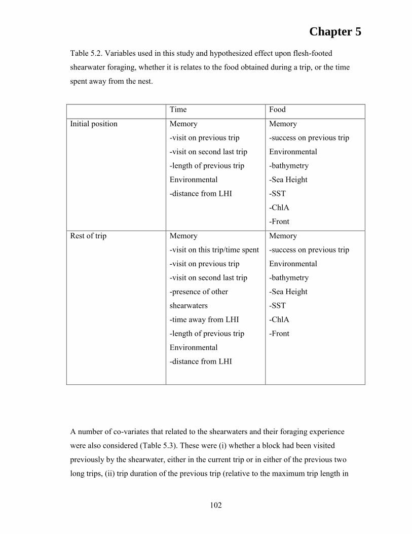
http://www.marine.csiro.au/dods-data/bluelink/synTS/


Chapter 5

102

Table 5.2. Variables used in this study and hypothesized effect upon flesh-footed

shearwater foraging, whether it is relates to the food obtained during a trip, or the time

spent away from the nest.

Time Food

Initial position Memory

-visit on previous trip

-visit on second last trip

-length of previous trip

Environmental

-distance from LHI

Memory

-success on previous trip

Environmental

-bathymetry

-Sea Height

-SST

-ChlA

-Front

Rest of trip Memory

-visit on this trip/time spent

-visit on previous trip

-visit on second last trip

-presence of other

shearwaters

-time away from LHI

-length of previous trip

Environmental

-distance from LHI

Memory

-success on previous trip

Environmental

-bathymetry

-Sea Height

-SST

-ChlA

-Front

A number of co-variates that related to the shearwaters and their foraging experience

were also considered (Table 5.3). These were (i) whether a block had been visited

previously by the shearwater, either in the current trip or in either of the previous two

long trips, (ii) trip duration of the previous trip (relative to the maximum trip length in

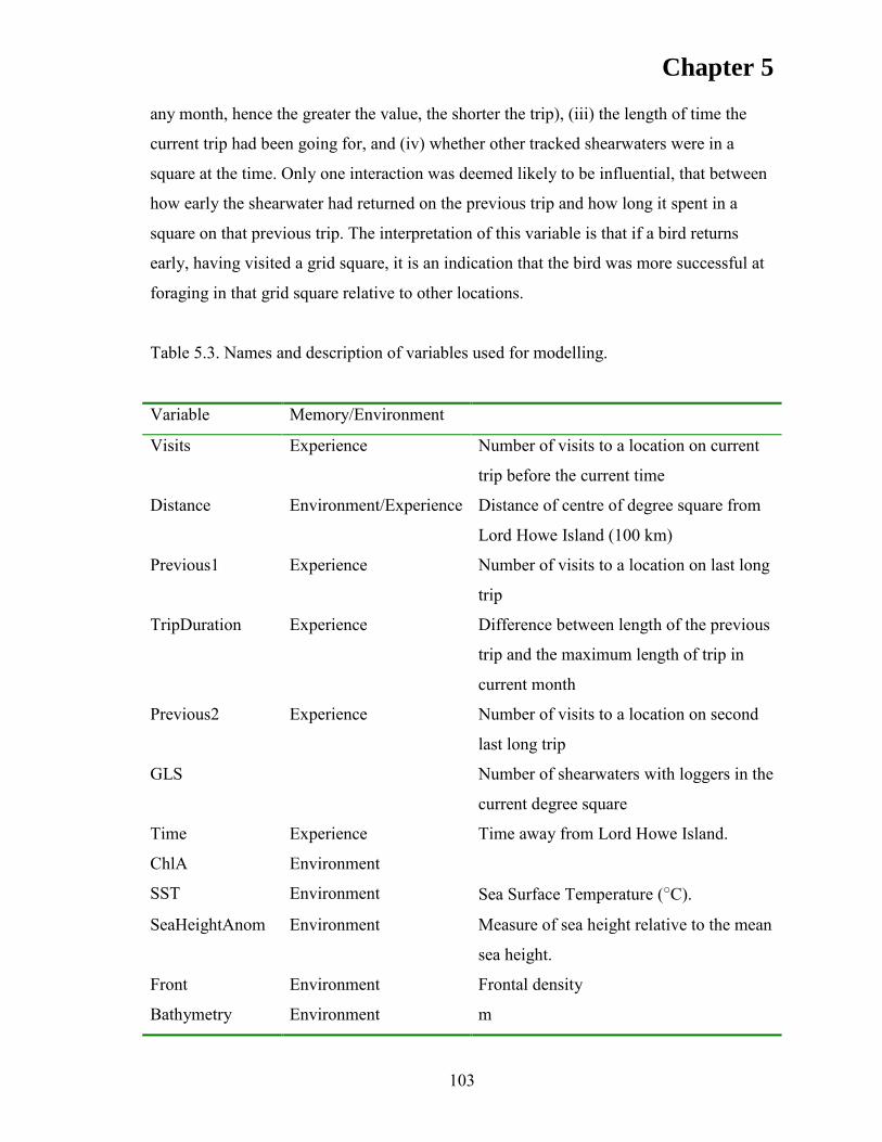
Chapter 5

103

any month, hence the greater the value, the shorter the trip), (iii) the length of time the

current trip had been going for, and (iv) whether other tracked shearwaters were in a

square at the time. Only one interaction was deemed likely to be influential, that between

how early the shearwater had returned on the previous trip and how long it spent in a

square on that previous trip. The interpretation of this variable is that if a bird returns

early, having visited a grid square, it is an indication that the bird was more successful at

foraging in that grid square relative to other locations.

Table 5.3. Names and description of variables used for modelling.

Variable Memory/Environment

Visits Experience Number of visits to a location on current

trip before the current time

Distance Environment/Experience Distance of centre of degree square from

Lord Howe Island (100 km)

Previous1 Experience Number of visits to a location on last long

trip

TripDuration Experience Difference between length of the previous

trip and the maximum length of trip in

current month

Previous2 Experience Number of visits to a location on second

last long trip

GLS Number of shearwaters with loggers in the

current degree square

Time Experience Time away from Lord Howe Island.

ChlA Environment

SST Environment Sea Surface Temperature (oC).

SeaHeightAnom Environment Measure of sea height relative to the mean

sea height.

Front Environment Frontal density

Bathymetry Environment m

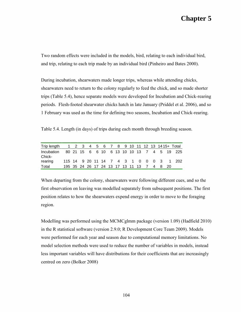
Chapter 5

104

Two random effects were included in the models, bird, relating to each individual bird,

and trip, relating to each trip made by an individual bird (Pinheiro and Bates 2000).

During incubation, shearwaters made longer trips, whereas while attending chicks,

shearwaters need to return to the colony regularly to feed the chick, and so made shorter

trips (Table 5.4), hence separate models were developed for Incubation and Chick-rearing

periods. Flesh-footed shearwater chicks hatch in late January (Priddel et al. 2006), and so

1 February was used as the time for defining two seasons, Incubation and Chick-rearing.

Table 5.4. Length (in days) of trips during each month through breeding season.

Trip length 1 2 3 4 5 6 7 8 9 10 11 12 13 14 15+ Total

Incubation 80 21 15 6 6 10 6 13 10 10 13 7 4 5 19 225

Chick-rearing 115 14 9 20 11 14 7 4 3 1 0 0 0 3 1 202

Total 195 35 24 26 17 24 13 17 13 11 13 7 4 8 20

When departing from the colony, shearwaters were following different cues, and so the

first observation on leaving was modelled separately from subsequent positions. The first

position relates to how the shearwaters expend energy in order to move to the foraging

region.

Modelling was performed using the MCMCglmm package (version 1.09) (Hadfield 2010)

in the R statistical software (version 2.9.0; R Development Core Team 2009). Models

were performed for each year and season due to computational memory limitations. No

model selection methods were used to reduce the number of variables in models, instead

less important variables will have distributions for their coefficients that are increasingly

centred on zero (Bolker 2008)

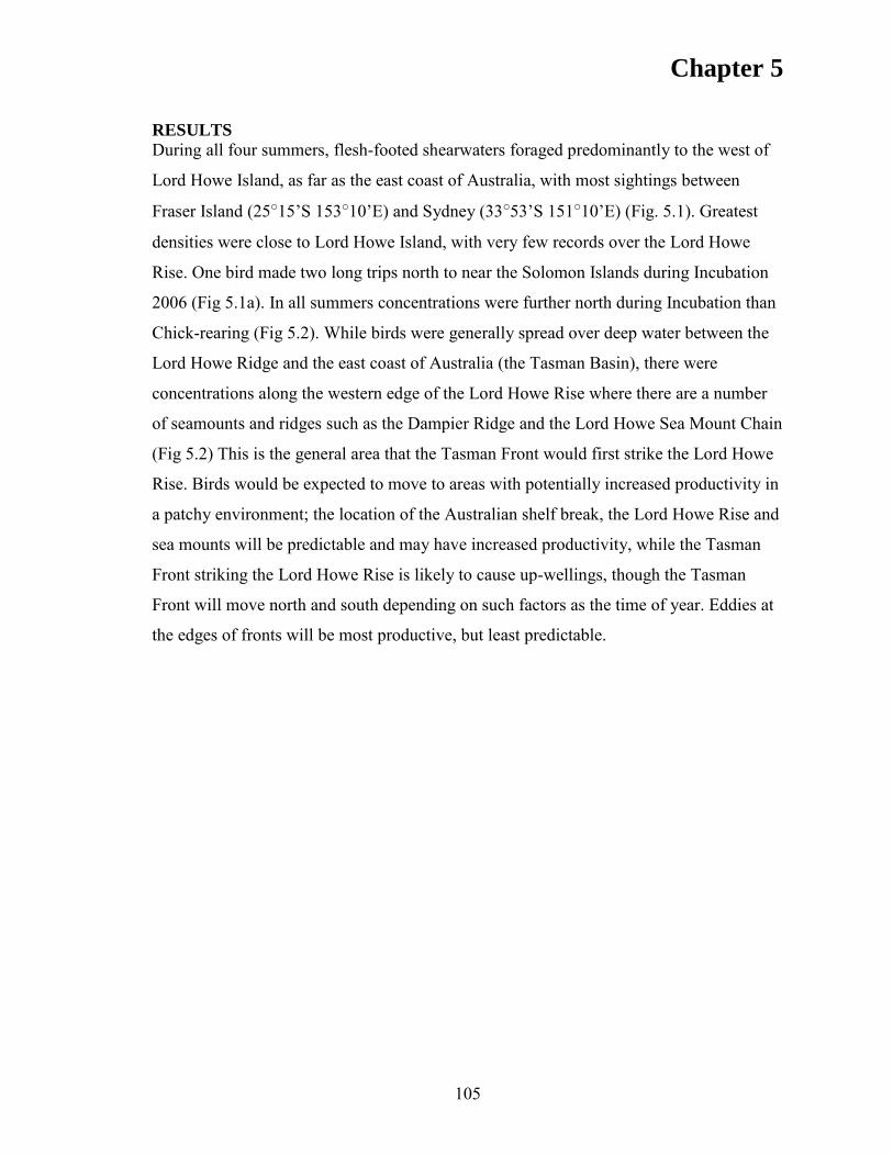
Chapter 5

105

RESULTS

During all four summers, flesh-footed shearwaters foraged predominantly to the west of

Lord Howe Island, as far as the east coast of Australia, with most sightings between

Fraser Island (25o15‟S 153o10‟E) and Sydney (33o53‟S 151o10‟E) (Fig. 5.1). Greatest

densities were close to Lord Howe Island, with very few records over the Lord Howe

Rise. One bird made two long trips north to near the Solomon Islands during Incubation

2006 (Fig 5.1a). In all summers concentrations were further north during Incubation than

Chick-rearing (Fig 5.2). While birds were generally spread over deep water between the

Lord Howe Ridge and the east coast of Australia (the Tasman Basin), there were

concentrations along the western edge of the Lord Howe Rise where there are a number

of seamounts and ridges such as the Dampier Ridge and the Lord Howe Sea Mount Chain

(Fig 5.2) This is the general area that the Tasman Front would first strike the Lord Howe

Rise. Birds would be expected to move to areas with potentially increased productivity in

a patchy environment; the location of the Australian shelf break, the Lord Howe Rise and

sea mounts will be predictable and may have increased productivity, while the Tasman

Front striking the Lord Howe Rise is likely to cause up-wellings, though the Tasman

Front will move north and south depending on such factors as the time of year. Eddies at

the edges of fronts will be most productive, but least predictable.

Chapter 5

106

a. b.

Fig 5.1 Distribution of all estimated positions of flesh-footed shearwaters during four

breeding seasons (2004/5, 2006/7, 2007/8 and 2008/9) (a). Twilight positions of all

archival tags in four summers. (b). Kernel density plot of all positions of flesh-footed

shearwaters from all summers.

Mean travel speeds varied between years, but not between seasons (Fig. 5.3; Table 5.5).

Mean distances that birds travelled from Lord Howe Island also varied within and

between years, with birds travelling significantly further from the island during

Incubation than during Chick-rearing period (Fig. 5.4; Table 5.6). Trips were also longer

during the Incubation period than the Chick-rearing period, with most trips being less

than seven days long (Table 5.4). The variance of trip lengths was also greater during the

Incubation period (Table 5.4).

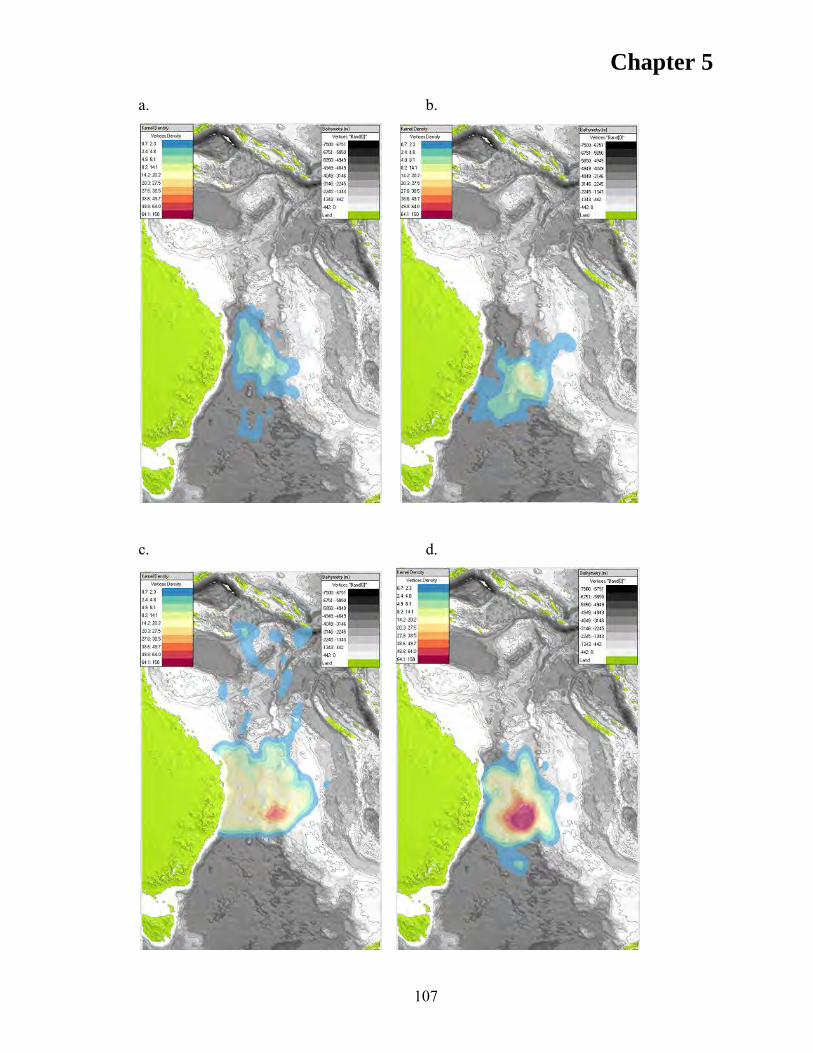
Chapter 5

107

a. b.

c. d.

Chapter 5

108

e.

f. g.

Chapter 5

109

Fig 5.2. Kernel density plots of distributions of flesh-footed shearwaters during each year

and season between 2004-2008. (Years aligned horizontally, seasons aligned vertically

(Incubation then Chick-rearing). (a). Incubation 2004. (b). Chick-rearing 2004. (c).

Incubation 2006. (d). Incubation 2007. (e). Chick-rearing 2007. (f). Incubation 2008. (g).

Chick-rearing 2008.

Fig 5.3. Mean (+1 standard deviation) observed speed (km hr-1) of flesh-footed

shearwaters for each year and season for long trips (>4 days).

Table 5.5. Fixed terms for speed (km/hr with log transformation) for different years and

two seasons (Intercept term for Chick-rearing in 2004). Random terms for model were

bird and trip.

Value Std.Error DF t-value p-value

Intercept 1.46 0.10 2894 14.86 <0.01

Year 2006 0.19 0.18 38 1.08 0.29

Year 2007 -0.33 0.15 38 -2.18 0.04

Year 2008 0.79 0.29 38 2.70 0.01

Incubation 0.00 0.05 2894 -0.05 0.96

Mean s

peed (

km

/hr)

05

10

15

20

25

2004 2006 2007 2008

Incubation

Chicks

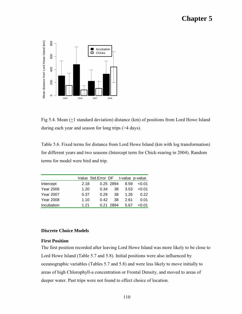
Chapter 5

110

Fig 5.4. Mean (+1 standard deviation) distance (km) of positions from Lord Howe Island

during each year and season for long trips (>4 days).

Table 5.6. Fixed terms for distance from Lord Howe Island (km with log transformation)

for different years and two seasons (Intercept term for Chick-rearing in 2004). Random

terms for model were bird and trip.

Value Std.Error DF t-value p-value

Intercept 2.18 0.25 2894 8.59 <0.01

Year 2006 1.20 0.34 38 3.53 <0.01

Year 2007 0.37 0.29 38 1.26 0.22

Year 2008 1.10 0.42 38 2.61 0.01

Incubation 1.21 0.21 2894 5.67 <0.01

Discrete Choice Models

First Position

The first position recorded after leaving Lord Howe Island was more likely to be close to

Lord Howe Island (Table 5.7 and 5.8). Initial positions were also influenced by

oceanographic variables (Tables 5.7 and 5.8) and were less likely to move initially to

areas of high Chlorophyll-a concentration or Frontal Density, and moved to areas of

deeper water. Past trips were not found to effect choice of location.

Mean d

ista

nce f

rom

Lord

How

e I

sla

nd (

km

)

0200

400

600

800

2004 2006 2007 2008

Incubation

Chicks

Chapter 5

111

Table 5.7. Model coefficients for first position after leaving Lord Howe Island for flesh-

footed shearwaters during Incubation Period (before 1 February). Highlighted numbers

are for those that were significant at a 95% level, as shown by the 2.5-97.5% MCMC

confidence limits not including zero.

2004 2006 2008

Coefficients Mean SD 2.50%

97.50

% Mean SD

2.50

%

97.50

% Mean SD

2.50

%

97.50

%

Intercept 20.30

16.4

3 -11.38 50.70 -0.30 5.13

-

10.26 9.80 -3.53 7.50

-

18.25 10.30

Visits

Distance -2.55 0.90 -4.24 -0.86 -1.31 0.57 -2.52 -0.38 0.89 0.91 -0.84 2.73

Distance^2 0.15 0.09 -0.06 0.32 -0.08 0.09 -0.20 0.15 -0.48 0.12 -0.71 -0.28

Previous1 -0.48 3.71 -8.36 6.18 -0.39 0.45 -1.31 0.40 -2.13 1.50 -5.15 0.39

TripDuration -0.35 0.30 -0.94 0.26 -0.02 0.05 -0.11 0.08 0.00 0.07 -0.13 0.14

Previous2 0.00 0.23 -0.49 0.41 0.55 0.38 -0.25 1.23

GLS -1.51 1.52 -4.95 0.94 0.25 0.34 -0.48 0.84

-

33.25

17.8

2

-

68.29 -4.44

Time

ChlA

-

90.84

35.1

3

-

151.9

0 -21.45

-

19.57

12.0

8

-

45.15 1.68

-

22.96

10.5

3

-

43.08 -3.17

SST -0.52 0.61 -1.59 0.68 -0.03 0.20 -0.40 0.38 -0.10 0.32 -0.72 0.54

SeaHeightAnom -3.74 3.51 -9.72 3.11 -3.23 2.55 -7.79 1.96 -3.45 3.62

-

10.09 3.31

Front -6.30 2.89 -12.28 -1.32 -1.54 0.91 -3.76 -0.01 -1.64 0.90 -3.59 -0.27

Bathymetry(x100) -0.09 0.00 -0.19 0.01 -0.09 0.02 -0.14 -0.05 -0.57 0.12 -0.81 -0.37

Previous1*TripDurati

on -0.07 0.93 -2.32 1.60 0.04 0.03 -0.02 0.11 0.22 0.13 0.00 0.50

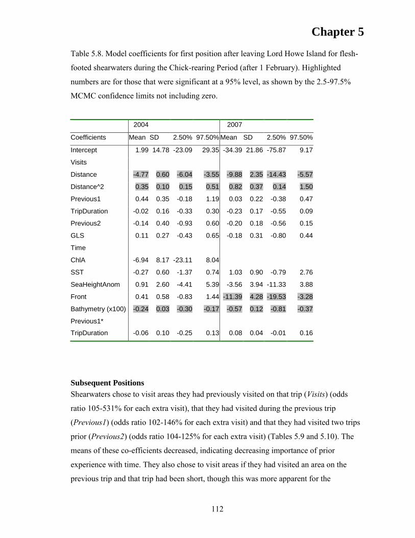
Chapter 5

112

Table 5.8. Model coefficients for first position after leaving Lord Howe Island for flesh-

footed shearwaters during the Chick-rearing Period (after 1 February). Highlighted

numbers are for those that were significant at a 95% level, as shown by the 2.5-97.5%

MCMC confidence limits not including zero.

2004 2007

Coefficients Mean SD 2.50% 97.50% Mean SD 2.50% 97.50%

Intercept 1.99 14.78 -23.09 29.35 -34.39 21.86 -75.87 9.17

Visits

Distance -4.77 0.60 -6.04 -3.55 -9.88 2.35 -14.43 -5.57

Distance^2 0.35 0.10 0.15 0.51 0.82 0.37 0.14 1.50

Previous1 0.44 0.35 -0.18 1.19 0.03 0.22 -0.38 0.47

TripDuration -0.02 0.16 -0.33 0.30 -0.23 0.17 -0.55 0.09

Previous2 -0.14 0.40 -0.93 0.60 -0.20 0.18 -0.56 0.15

GLS 0.11 0.27 -0.43 0.65 -0.18 0.31 -0.80 0.44

Time

ChlA -6.94 8.17 -23.11 8.04

SST -0.27 0.60 -1.37 0.74 1.03 0.90 -0.79 2.76

SeaHeightAnom 0.91 2.60 -4.41 5.39 -3.56 3.94 -11.33 3.88

Front 0.41 0.58 -0.83 1.44 -11.39 4.28 -19.53 -3.28

Bathymetry (x100) -0.24 0.03 -0.30 -0.17 -0.57 0.12 -0.81 -0.37

Previous1*

TripDuration -0.06 0.10 -0.25 0.13 0.08 0.04 -0.01 0.16

Subsequent Positions

Shearwaters chose to visit areas they had previously visited on that trip (Visits) (odds

ratio 105-531% for each extra visit), that they had visited during the previous trip

(Previous1) (odds ratio 102-146% for each extra visit) and that they had visited two trips

prior (Previous2) (odds ratio 104-125% for each extra visit) (Tables 5.9 and 5.10). The

means of these co-efficients decreased, indicating decreasing importance of prior

experience with time. They also chose to visit areas if they had visited an area on the

previous trip and that trip had been short, though this was more apparent for the

Chapter 5

113

Incubation than the Chick-rearing period (Previous1*TripDuration) (Tables 5.9 and

5.10). They were less likely to visit areas the further the area was from Lord Howe Island.

They were less likely to visit any areas the longer the trip went, indicating there was some

likely maximum to the length of trips. During one of four years in Incubation (Table 5.9)

and two of three years in Chick-rearing the number of other shearwaters with loggers

(GLS) showed a positive relationship with choosing to visit an area, though this included

zero (Table 5.10), while in other years and seasons the relationship was centred on zero.

Flesh-footed shearwaters were more likely to visit an area with increasing Sea Height

Anomaly (odds ratio 107-191% for each increase of 1 cm) (Tables 5.9 and 5.10). Sea

Height Anomaly had a mean of 0.05 cm (s.d. 0.12). During incubation, they were more

likely to visit an area with increasing Sea Surface Temperature (odds ratio 103-132% for

each 1oC), but less likely to visit in the Chick-rearing period (odds ratio 6-97%). During

Incubation they were less likely visit an area with increasing Chlorophyll-a (odds ratio

<0.1-1%). Chlorophyll-a had a mean of 0.09 mg m-3 (s.d. 0.11). Frontal density showed

little pattern.

Comparing the means of the coefficients of the experience and oceanographic variables

(Table 9), during Incubation for Sea Height Anomaly, the increase in likelihood of

visiting an area was approximately one third for each 1 cm of rise compared to each

previous visit, it was also approximately one third for each 1oC rise in Sea Surface

Temperature and was approximately 20 times for each fall of 1 mg m-3 of Chlorophyll-a.

During Chick-rearing (Table 5.10), the increase in likelihood of visiting an area was

similar for one visit, an increase of 1 cm of Sea Height Anomaly, a fall of 1oC in Sea

Surface Temperature. The mean for Chlorophyll-a for a fall of 1 mg m-3 was

approximately ten times that for a single visit.

Chapter 5

114

Table 5.9. Model coefficients for subsequent positions during Incubation Period (before 1 February). Highlighted numbers are

for those that were significant at a 95% level, as shown by the 2.5-97.5% MCMC confidence limits not including zero.

2004 2006 2007 2008

Coefficients Mean SD 2.50% 97.50% Mean SD 2.50% 97.50% Mean SD 2.50% 97.50% Mean SD 2.50% 97.50%

Intercept -13.47 3.58 -19.72 -5.90 -4.05 0.99 -6.01 -2.15 -7.33 0.73 -8.66 -5.83 -2.06 2.43 -4.88 1.15

Visits 0.98 0.13 0.72 1.23 0.55 0.03 0.50 0.60 0.47 0.02 0.44 0.51 0.66 0.07 0.51 0.81

Distance -0.74 0.20 -1.13 -0.34 -0.76 0.07 -0.90 -0.62 -1.02 0.08 -1.16 -0.87 -0.21 0.11 -0.41 0.02

Distance^2 0.03 0.02 -0.01 0.07 0.04 0.01 0.03 0.06 0.05 0.01 0.03 0.07 -0.01 0.01 -0.04 0.01

Previous1 -1.34 0.92 -3.26 0.31 0.28 0.05 0.18 0.38 0.08 0.03 0.02 0.15 0.10 0.08 -0.05 0.24

TripDuration -0.03 0.12 -0.28 0.19 0.01 0.01 -0.01 0.03 -0.01 0.01 -0.02 0.01 -0.01 0.01 -0.04 0.01

Previous2 0.15 0.03 0.09 0.21 0.08 0.02 0.04 0.12 0.11 0.08 -0.04 0.26

GLS 0.48 0.27 -0.05 0.99 -0.04 0.10 -0.23 0.15 0.03 0.06 -0.08 0.14 0.00 0.34 -0.66 0.60

Time -0.05 0.03 -0.11 0.02 -0.02 0.01 -0.03 -0.01 -0.04 0.00 -0.05 -0.03 -0.02 0.01 -0.03 0.00

ChlA -2.90 6.71 -16.44 9.70 -9.26 2.42 -13.67 -4.26 -13.88 2.38 -18.76 -8.46

SST 0.38 0.48 -0.55 1.36 0.14 0.06 0.03 0.26 0.17 0.05 0.07 0.28 -0.21 0.08 -0.37 -0.07

SeaHeightAnom 0.41 0.13 0.14 0.65 0.03 0.04 -0.04 0.11 0.13 0.03 0.07 0.19 -0.06 0.04 -0.14 0.03

Front -0.58 1.01 -2.47 1.43 -2.28 0.53 -3.27 -1.15 2.20 0.30 1.63 2.81 -0.29 0.60 -1.45 0.84

Bathymetry

(x100) -0.03 0.01 -0.06 -0.01 -0.04 0.01 -0.05 -0.03 -0.06 0.00 -0.06 -0.05 -0.03 0.01 -0.04 -0.02

Previous1*

TripDuration 0.46 0.21 0.05 0.92 -0.01 0.00 -0.02 0.00 0.00 0.00 0.00 0.01 0.04 0.02 0.01 0.06

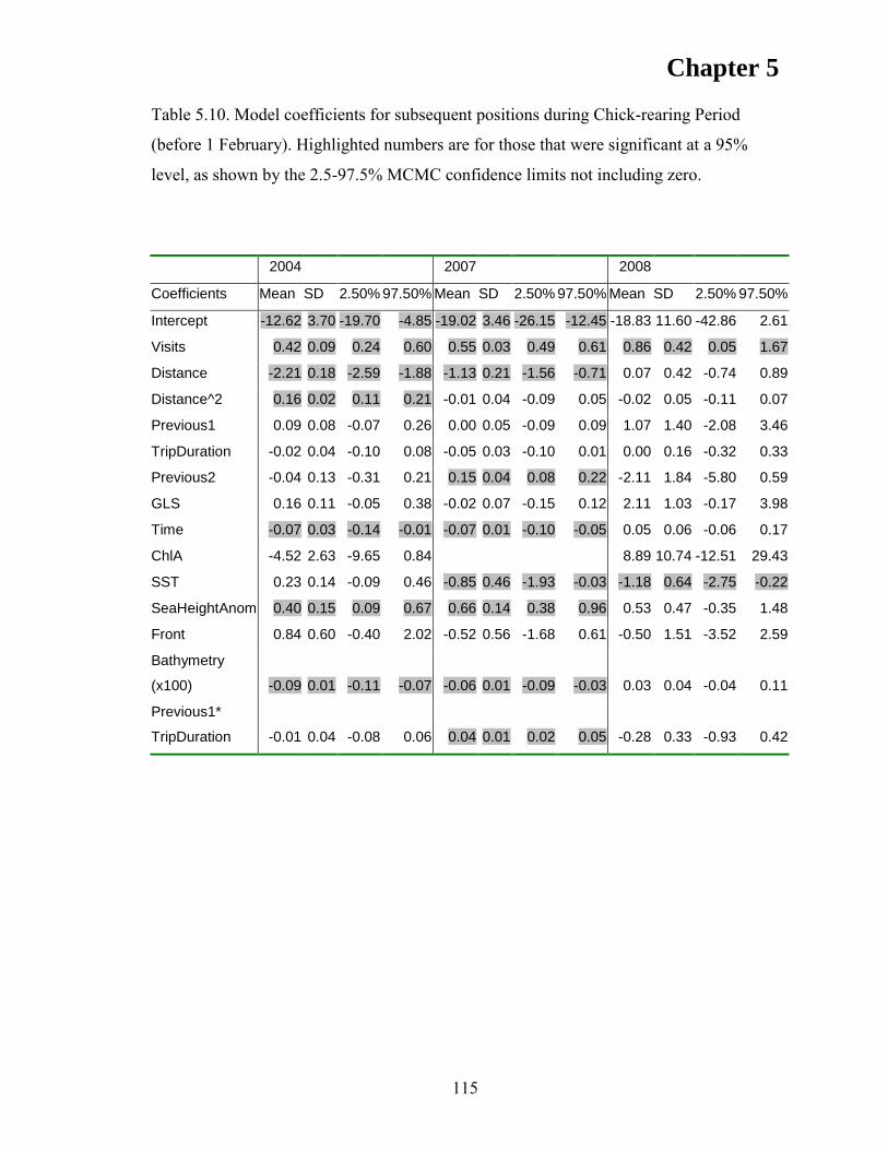
Chapter 5

115

Table 5.10. Model coefficients for subsequent positions during Chick-rearing Period

(before 1 February). Highlighted numbers are for those that were significant at a 95%

level, as shown by the 2.5-97.5% MCMC confidence limits not including zero.

2004 2007 2008

Coefficients Mean SD 2.50% 97.50% Mean SD 2.50% 97.50% Mean SD 2.50% 97.50%

Intercept -12.62 3.70 -19.70 -4.85 -19.02 3.46 -26.15 -12.45 -18.83 11.60 -42.86 2.61

Visits 0.42 0.09 0.24 0.60 0.55 0.03 0.49 0.61 0.86 0.42 0.05 1.67

Distance -2.21 0.18 -2.59 -1.88 -1.13 0.21 -1.56 -0.71 0.07 0.42 -0.74 0.89

Distance^2 0.16 0.02 0.11 0.21 -0.01 0.04 -0.09 0.05 -0.02 0.05 -0.11 0.07

Previous1 0.09 0.08 -0.07 0.26 0.00 0.05 -0.09 0.09 1.07 1.40 -2.08 3.46

TripDuration -0.02 0.04 -0.10 0.08 -0.05 0.03 -0.10 0.01 0.00 0.16 -0.32 0.33

Previous2 -0.04 0.13 -0.31 0.21 0.15 0.04 0.08 0.22 -2.11 1.84 -5.80 0.59

GLS 0.16 0.11 -0.05 0.38 -0.02 0.07 -0.15 0.12 2.11 1.03 -0.17 3.98

Time -0.07 0.03 -0.14 -0.01 -0.07 0.01 -0.10 -0.05 0.05 0.06 -0.06 0.17

ChlA -4.52 2.63 -9.65 0.84 8.89 10.74 -12.51 29.43

SST 0.23 0.14 -0.09 0.46 -0.85 0.46 -1.93 -0.03 -1.18 0.64 -2.75 -0.22

SeaHeightAnom 0.40 0.15 0.09 0.67 0.66 0.14 0.38 0.96 0.53 0.47 -0.35 1.48

Front 0.84 0.60 -0.40 2.02 -0.52 0.56 -1.68 0.61 -0.50 1.51 -3.52 2.59

Bathymetry

(x100) -0.09 0.01 -0.11 -0.07 -0.06 0.01 -0.09 -0.03 0.03 0.04 -0.04 0.11

Previous1*

TripDuration -0.01 0.04 -0.08 0.06 0.04 0.01 0.02 0.05 -0.28 0.33 -0.93 0.42

Chapter 5

116

DISCUSSION

We have shown that a central place foraging marine predator (the flesh-footed

shearwater) chose to return to areas that they have previously been, suggesting that

experience is influencing their choice of foraging area. Because their food resources are

distributed patchily, choosing to forage somewhere that has already been used

successfully offers clear advantages. However, this has only rarely been demonstrated.

Black-legged kittiwakes Rissa tridactyla made an average of two trips per day to tidal

fronts in Prince William Sound, Alaska (Irons 1998). Northern gannets (Morus bassanus)

and red-footed boobies repeatedly departed their colonies in the same directions (Lewis et

al. 2002; Weimerskirch et al. 2005). Northern fur-seals and southern elephant seals return

to similar areas between foraging trips, from one year to the next (Bradshaw et al. 2004;

Call et al. 2008).

The effect of experience was greater in the Incubation period than during the Chick-

rearing period. They are less constrained in terms of time during Incubation, therefore

they have more opportunity to find higher quality areas, which can be exploited on

subsequent trips. In Chick-rearing, with less search time, the quality of the information

may be less and therefore more readily discarded. Further, we have only considered

longer trips. Thus in the Chick-rearing period, there may have been some short trips since

the previous long trip. This may have diluted the memory of the previous long trip, either

by increasing the time since the last long trip, or by creating memories of short trips in

between.

At the scale used in this study, the experience variables were at least as important as

oceanographic variables. Further, the oceanographic variables were not affecting choice

in ways obviously corresponding to increased productivity. This may be scale related. In

the Mozambique Channel, breeding great frigate-birds Fregata minor used sub-

mesoscale surface mixing and transport structures (Lagrangian Coherent Structures)

along the edges of eddies when foraging (Tew Kai et al. 2008). However, it was unknown

how the frigate-birds located the areas, as they were up to 1,000 km from the breeding

grounds (Tew Kai et al. 2008). These types of structures are also present in the East

Chapter 5

117

Australia Current and Tasman Front between Lord Howe Island and the east coast of

Australia (Waugh et al. 2006), in areas to which the shearwaters were returning.

Learning increases foraging efficiency in bluegill sunfish Lepomis macrochirus and

bumblebees Bombus terrestris (Werner et al. 1981; Peat and Goulson 2005). Although,

these species forage over relatively short distances it would be similarly beneficial for a

longer distance central place forager such as flesh-footed shearwaters. Search strategies

such as correlated random walks have been hypothesized as the most efficient ways to

find food in an environment with patchy resources (Viswanathan et al. 1996; Fauchald

and Tveraa 2003; Tremblay et al. 2007) in the absence of other information, but if

predators are able to reduce the area that needs to be searched through experience, this is

going to greatly increase the efficiency of that predator. Minimising the time spent

searching is advantageous by optimal foraging theory; by minimising the time spent

searching the forager should also be able to minimise the time required to feed within a

patch, or alternatively allow them to spend more time in a coarse scale patch to search for

the areas of high productivity at the edges of eddies within this patch (Charnov 1976).

The shearwaters apparently use experience in a dynamic way, because the probability of

visiting an area declined with the time since the last visit, suggesting the shearwaters

discount the information they have gained with increasing time since they gained it.

Bumblebee's memories of where they were foraging the previous day declines overnight,

though not completely (Keaser et al. 1996). Alternatively, because the shearwaters were

returning to productive areas on an ocean, the features are likely to be dynamic, and

hence, they may have moved or degraded. Nevertheless, shearwaters with loggers

foraged in approximately similar areas (to the west of Lord Howe Island) in different

years, suggesting that experience at some scale still determines where the shearwaters go

(Fig. 1). This indicates the effect of experience varies with the scale examined. At large

scales, features such as the breeding site on Lord Howe Island and the Tasman Sea are

highly predictable; but as scale declines, so does the predictability of features. While

seamounts are also predictable, the currents that cause up-wellings around them shift in

location and strength. At the smallest scale, that of eddies, features have lifetimes on the

Chapter 5

118

order of days to months, and thus could change substantially over the course of a few

foraging trips.

The coarse scale used here for areas that the shearwaters were returning to have shown

low levels of correspondence between spatial distribution of seabirds and zooplankton

(Reid and Hindell 2000). Therefore, while they apparently use experience to get to areas

they have previously visited and were more likely to have successfully foraged, once they

are in the area, they must find food. Food is likely to be related to fine scale, dynamic

features that are found within the coarse scale features that they are visiting using

memory. Presumably this is when they adopt different means to find food, such as smell

(Nevitt et al. 2008) or sighting other marine predators (Au and Pitman 1986; Haney et al.

1992). Scale is very important in analysing the distribution of foraging seabirds and their

prey (Fauchald et al. 2000). Fauchald et al. (2000) hypothesised a hierarchical search

pattern so that murres searched initially in a large-scale manner with long travel distances

and low turning angles, and once within a large-scale patch they searched by using

shorter travel distances and sharp turning angles. These larger scale searches could be

analogous to the flesh-footed shearwaters using experience to find foraging areas. There

may be two processes involved rather than one, with shearwaters choosing to go to an

area, and then searching, rather than searching from the start.

The shearwaters were exhibiting a range of time scales for foraging. Most recent

experience was also likely to be closest experience, so they used this at a large scale to

determine where to go, but then at a fine scale as they are foraging to make decisions

about whether to accept a new location or return to a location they visited earlier on the

same trip. Experience of previous foraging areas is only useful if there is some chance of

the feature they are returning to remaining where it was (or nearby). This is likely to vary

depending on the feature. Ideally if a patch of food occurs permanently in some position,

experience will be a very efficient manner to return to it. This would be a quite rare

situation in the marine environment (though it may be approximated by tidal fronts (Irons

1998) or sea mounts). However, if food will intermittently occur in some general area,

experience may assist the predator to find that general area, but other cues may be

Chapter 5

119

necessary to find the actual food at the time the predator is there. This is likely to be the

situation with oceanographic features such as currents and eddies that occur within the

Tasman Sea (Ridgeway and Dunn 2003). These features often generate areas of increased

productivity, and patches of prey. However, the prey patches will not be permanent and

so will move around in the general area that they have occurred. Further to this, over

time, features such as these will degrade and move on to other areas. Therefore for this

situation, it is useful for the information gained from experience to degrade also. At the

opposite extreme to permanent features is totally (or near) random features, and for these

experience of locations is useless.

Flesh-footed shearwaters were predominantly using experience, however, they were also

choosing areas used by other tracked individuals. This may have been due to the

shearwaters moving to similar areas due to other cues, or to their following congeners.

Black-legged kittiwakes predominantly used experience to choose where to forage,

apparently not using information from other birds (Irons 1998). The weakness of the

relationship for the shearwaters may have indicated they only formed flocks for some of

the time (perhaps in some years or seasons and not others), or that there were insufficient

data (low number of tracked birds) to form a stronger pattern. This could be better tested

using proximity loggers (Ji et al. 2005).

We used discrete choice models in an ecological context, because they allow the

combination of environmental data and behavioural decisions, such as whether to return

to an area, or which prey to hunt. Discrete choice models have been used in several other

ecological situations: oceanographic preference of bluefin tuna (Teo et al. 2007), hunting

decisions of cheetahs (Cooper et al. 2007), and resource selection by elk Cervus elaphus

(Cooper and Millspaugh 1999).

CONCLUSIONS

At a coarse scale, flesh-footed shearwaters breeding on Lord Howe Island were using

experience and the quality of the information they had to determine their choice of

foraging area. They were more likely to visit an area the more often they had visited it

Chapter 5

120

during the current, or two previous trips; however the likelihood of returning became less

the longer it was since a previous visit. This indicates that they were using previous

experience, but that the birds discounted this information as it aged. We expect this to be

an adaptive trait, given that the birds forage on ephemeral features such as the edges of

eddies in oceanic fronts. Thus it is useful to „remember‟ where a productive patch was in

the immediate past, but the usefulness of this information decreases with time as the

patches move and change. The use of experience by shearwaters is important in the

understanding of how marine predators forage, as it should increase the foraging

efficiency of the shearwaters, and allow them to utilize the other tools available to them,

such as efficient search methods (e.g. area restricted search or Levy flights) or using

environmental cues (smell or sight), in much smaller areas. Our results suggest that

experience and memory may overwhelm the role of oceanographic variables in driving

the foraging distribution of marine predators. The implication of this is that the search

for predictive models of species distributions in marine systems based on remotely sensed

data such as sea surface colour may never yield high quality predictive models.

Chapter 5

121

ACKNOWLEDGEMENTS

Jennifer Lavers, Drew Lee, Peter Vertigan, Sam Thalmann, Michele Thums, Laurel

Johnston, Ray Murphy, Glen Dunshea, Rhonda Pike assisted during field work. Remote

sensing data was supplied by the Commonwealth Scientific and Industrial Research

Organisation (CSIRO). NCEP reanalysis data provided by the NOAA-CIRES Climate

Diagnostics Center, Boulder, Colorado, USA, from their Web site at

http://www.cdc.noaa.gov/. This study was supported by a joint CSIRO/University of

Tasmania QMS joint scholarship. Work on shearwaters was conducted under the

University of Tasmania Animal Ethics Committee Project number A0009154 and New

South Wales Department of Climate Change permit number S12408.

Chapter 6

122

6. General Discussion and synthesis of results

The aim of this thesis was to investigate the continuing trends in the Lord Howe Island

population of flesh-footed shearwaters, and how these trends were related to fisheries

interactions and oceanography. Previously, the population had been shown to be

declining, with habitat clearing and fisheries by-catch in the ETBF highlighted as likely

contributing factors (Baker and Wise 2005; Priddel et al. 2006). The methods used for

mitigating seabird by-catch were largely unsuccessful for this species (Baker and Wise

2005), most likely due to its manoeuvrability and deep diving ability (Brothers et al.

1999). This study has produced considerable new information on the status of the Lord

Howe Island population of Lord Howe Island, and the threats it is facing, as well as

suggesting means to mitigate fisheries by-catch, based on data on the at-sea distribution

of the birds, and the factors that influence this. In spite of recent decreases in fisheries by-

catch and land clearing, the population has continued to decline, with extra mortality

noted on roads on the island (Chapter 2). Declining by-catch in the tuna fishery in the

region can be explained by decreasing overlap between the fishery and the foraging

shearwaters (Chapter 3); the shearwaters predominantly foraged in potentially rich areas

(Chapter 4); and returned to similar areas over successive trips, indicating the use of

experience to choose where to forage (Chapter 5). These results suggest the shearwaters

are returning to approximately the same productive areas, indicating the use of closures

of quite specific areas has the potential to be effective as a mitigation measure.

The results were interpreted in their own particular context at the end of each chapter,

while this discussion will provide a synthesis of the findings, especially with regards the

possibility of the results‟ use for mitigation of fisheries by-catch for species for which

other more standard mitigation techniques have not worked.

Population trend

Chapter 2 demonstrated a posterior probability of 0.85 that the population is continuing to

decline. Two sources implicated in the decline from 1978-2002 were breeding habitat

Chapter 6

123

loss on Lord Howe Island, and mortality in fisheries of the ETBF (Baker and Wise 2005;

Priddel et al. 2006). However, the loss of breeding habitat had ceased over the 2002-2009

period, thus suggesting this was no longer the problem or that there is a time lagged effect

of the loss. There was some evidence of lower breeding success in parts of colonies that

were more disjointed. Further, there is now evidence to suggest that the rates of by-catch

mortality have declined in the ETBF (Trebilco et al. 2010). Therefore other sources of

mortality are apparently contributing to the decline.

During the summer of 2008/9 adult mortality of flesh-footed shearwaters on the roads on

Lord Howe Island was 129-262 (an estimated annual adult mortality of 0.2-0.4%;

Chapter 2). This is a similar magnitude to the current observed by-catch mortality rate

within the ETBF (Trebilco et al. 2010; Baker pers. comm.). There is also evidence of

plastics being consumed by the adults at sea and passed on to the chicks; though it

remains unclear what effect this is having on the population (Hutton et al. 2008; Chapter

2).

Spatial overlap with fisheries

Flesh-footed shearwater by-catch in the ETBF has fallen in recent years, therefore,

increasing our understanding of the spatial interactions with the fishery and how it may

influence by-catch will potentially help with management of future changes of by-catch

(Chapter 3). Counts of flesh-footed shearwaters behind vessels operating in the ETBF

were used to model the areas of spatial overlap over the period from 2001-2006. This was

done using a GLM approach. Overlap between the fishery and the flesh-footed

shearwaters predominantly occurred to the west and south-west of Lord Howe Island.

Using this model, in two of three years that the areas of interactions were predicted for

(1998 and 2002), interactions were high as a significant proportion of the fishery was

operating in the same area, targeting broadbill swordfish and yellowfin tuna. However, by

2006 most of the fishing effort was targeting albacore tuna, and operating well to the

north of Lord Howe Island, and so the overlap between the fishery and the shearwaters

was much reduced (Chapter 3). By-catch rates in the ETBF were much lower during this

latter period (Trebilco et al. 2010). This makes sense, as by-catch rates were correlated to

Chapter 6

124

the number of birds interacting with long-line vessels at the time of line setting (Trebilco

et al. 2010).

Thus, the decline in the by-catch rate for flesh-footed shearwaters in the ETBF

corresponds with the fishery shifting away from areas where the birds forage. The

apparent decline in the by-catch rate is based on observer coverage of less than 5% of

fishing effort (Trebilco et al. 2010). Hence there is much uncertainty in the estimated

decline in by-catch rate, in particular the accuracy and representativeness of the estimates

from such a small sample. A further issue is that the decline in by-catch rate has resulted

from fishers changing target species and fishing area; there is some probability that at

some time the fishers will change area and target species again and return to targeting

those that resulted in spatial overlap and subsequent high by-catch rates.

Foraging choices of shearwaters

The models used in Chapter 3 to identify overlap between the fisheries and flesh-footed

shearwaters are useful but limited. There are a number of limitations inherent in the

assumptions behind them, such as they are unable to deal with the autocorrelation

between successive counts in the data and they are linear in shape and so are unable to

completely reflect underlying beliefs about the relationships being modelled.

Understanding the drivers for flesh-footed shearwater foraging, in particular the role of

oceanographic conditions and experience, will improve knowledge of where shearwaters

forage and how they use the environment, and this will further assist in fishery

management. In order to do this, two novel statistical methods needed to be adapted.

In Chapter 4 a multi-component model was used to examine the abundance of flesh-

footed shearwaters attending vessels, modelling abundance as a sum of arrivals and

departures of individual birds at the vessel. This model was developed to reflect the

underlying process driving the observations of birds attending vessels, and was estimated

using maximum likelihood (Hilborn and Mangel 1997; Clark 2007; McCarthy 2007;

Bolker 2008). This approach better reflects our understanding of the system, facilitating

not only prediction but also learning. These more mechanistic statistical models are

Chapter 6

125

becoming more frequently used with the development of new ways to solve the

mathematical issues in the models through increased computer power, and are at the

cutting edge of analytical methods in ecology (McCarthy 2007).

By using an arrivals/departures models to analyse counts of flesh-footed shearwaters

behind fishing vessels, it is possible to quantify the effect of smaller scale cues such as

eddies or fish catch on attendance (Chapter 4). It is not possible to identify bird

interactions at these scales using observer data and the models used in Chapter 3. At

smaller scales, shearwaters were more likely to arrive behind fishing vessels when they

were operating in areas of up-wellings and down-wellings at the edges of eddies in the

Tasman Sea and along shelf-breaks. This suggested that the shearwaters were attending

the vessels when they were operating in productive areas. Therefore, more birds may be

attending the vessels due to there being more birds in the area, however they may only

attend fishing vessels as one of a number of potential food sources while they are

operating in the area the shearwaters had already chosen to forage. These patterns are

supported by results from other seabirds attending fishing vessels. In the Baltic Sea

seabirds were found to be much more responsive to changes in oceanographic conditions,

such as up-wellings, or prey, rather than the quantity of food available from trawlers

operating nearby (Skov and Durinck 2001). They found that the attraction of trawlers for

seabirds was only a local process (< 10 km). Westland petrels off New Zealand were

found to only attend fishing trawlers if they were operating in the areas the petrels

naturally chose to forage (Freeman 1997).

In Chapter 5 a multinomial logit model was used to determine where individual flesh-

footed shearwaters were foraging, and which factors were important in their choice.

These so-called discrete choice models rely on an animal making a choice, where only

one of a finite number of choices is possible at one time (Train 2003). In this context, the

model allows the shearwater‟s choice of foraging area to be dependent on environmental

and behavioural co-variates at the same time. Applications of this promising approach are

rare in ecology, although there are some examples such as in studies of factors relating to

hunting decisions by cheetahs (Cooper et al. 2007).

Chapter 6

126

During the breeding season, flesh-footed shearwaters generally foraged between the east

coast of Australia and the Lord Howe Rise, a ridge running north-south through the

Tasman Sea. Lord Howe Island is on the western edge of the ridge, and is in the region

that the Tasman Front strikes the ridge (Ridgeway and Dunn 2003). Most interactions

between fishing vessels in the ETBF and flesh-footed shearwaters also occurred to the

west of the Lord Howe Rise (Chapter 3). The birds chose to visit areas that they had

previously visited, including places that they had visited within the two previous trips. In

addition, they were visiting areas that they were more likely to have foraged successfully

in during the previous trip. The shearwaters were using previous experience to return to

areas known to be profitable. Experience has been hypothesised as a means for animals to

locate food, but only rarely demonstrated. Black-legged kittiwakes Rissa tridactyla

returned to the same area at tidal fronts in Prince William Sound (Irons 1998), while

northern fur-seals and southern elephant seals return to similar areas between foraging

trips (Bradshaw et al. 2004; Call et al. 2008). Learning from experience is beneficial as it

increases foraging efficiency (e.g. in bluegill sunfish Lepomis macrochirus and

bumblebees Bombus terrestris (Werner et al. 1981; Peat and Goulson 2005)). Experience

improved the foraging of a mobile crab, the blue crab Calinectes sapidus, but had no

effect on a sedentary crab, the Atlantic mud crab Panopeus herbsti (Micheli 1997). The

use of experience to locate patches can be thought of as fitting into optimal foraging

theory through minimising the time spent between patches as well as accumulating

information for future foraging success, especially for species with significant

movements to patches (Charnov 1976; Clark and Mangel 1984). The effect of experience

on the flesh-footed shearwaters decreased with passing time, indicating it was becoming

less useful. The patches they were most likely returning to were likely to be dynamic, and

hence it is useful to weight the usefulness of experience, with more recent experience

being more useful than older experience. Bumblebees have been shown to partially forget

experience overnight (Keaser et al. 1996). Learning is more useful for long lived foragers

such as flesh-footed shearwaters (Eliassen et al. 2007). It is also more useful in

temporally varied environments (Eliassen et al. 2009). This is likely to move closely

match the Tasman Sea environment and fronts as encountered by shearwaters. Learning

Chapter 6

127

the locations of previously encountered prey patches allows birds to increase foraging

efficiency, but forgetting allows for the use of a flexible foraging strategy (Eliassen et al.

2009).

Foraging scale

The results here (Chapters 4 and 5) suggest that flesh-footed shearwaters are foraging at a

range of scales. During all four summers for which data were collected, they were

foraging in approximately the same areas – predominantly between Lord Howe Island

and the east coast of Australia. But at a coarse scale (~100 km) they were significantly

likely to choose to remain in an area and return to that area on following trips. At smaller

scales the shearwaters were apparently remaining in areas that were most productive. At

sub-meso scales (<10 km), up-wellings of productive waters are formed at the edges of

eddies; great frigate-birds were shown to forage in these in the Mozambique Channel

(Tew Kai et al. 2008), while similar structures have been shown to occur in the same

areas that the flesh-footed shearwaters are choosing to return to (Waugh et al. 2006). It

can be hypothesised that the shearwaters are behaving in a similar way in the Tasman Sea

to how the frigate-birds were behaving, and thus using similar structures in the edges of

currents. Nevertheless, at coarse scales, the probability of choosing to return to an area

declined over time, indicating that, at least at that scale, the shearwaters were „forgetting‟

where they had been foraging. This is a useful characteristic due to the dynamic nature of

the sub-meso scale features, so that the quality of the information would degrade.

Scale is an important means to look at aspects of the ecology of marine predators, and

how they locate their food (Hunt and Schneider 1987). In the case of seabirds such as

flesh-footed shearwaters, at a large scale they spend their time within the possible

foraging range around Lord Howe Island. This could be viewed as a circle around Lord

Howe Island encompassing how far they can potentially fly and return (though, this is too

simplistic, as wind will also influence how far they can fly). However, within this, there

are probably areas that are unsuitable (such as areas of ocean that are unproductive).

Therefore, at coarse scales there are areas that have the potential to be productive (such as

eddies and fronts at the edges of currents, shelf breaks or sea mounts), and others that are

Chapter 6

128

unsuitable. Over shorter time scales eddies and fronts at the edges of currents are

relatively predictable as they move slowly enough such that they will remain in

approximately similar areas on the time scale of a foraging trip, and so it is advantageous

for foragers to return to them. Dynamic memory, which gives more weight to recent

experience, allows foragers to return to these ephemeral areas, potentially greatly

improving the efficiency of foraging effort. However, at smaller scales, productive areas

are unevenly and unpredictably distributed (i.e. there are not up-wellings along the

complete length of an eddy), therefore within coarse scale there is a need to locate the

productive areas. At this scale, the use of efficient search patterns (such as correlated

random walks) play an important role in predators foraging strategies.

A number of studies have used marine predators‟ movements to look at efficient search

patterns (Viswanathan et al. 1996; Fauchald and Tveraa 2003; Tremblay et al. 2007).

These studies have often used algorithms to look at animals moving a range of distances

(especially using power laws such as Lévy flights). They have suggested it is efficient to

be able to intermix longer and shorter movements (and changes of angle) in order to

cover the environment efficiently in search of food patches (Viswanathan et al. 1996).

However, these are using an essentially random process (hence the name correlated

random walks) and require little information about the environment to be held by the

forager. The use of experience has been shown to improve foraging efficiency in a

number of species (Chapter 5). The results here for the flesh-footed shearwater suggests

they use experience to return to similar areas, and so can greatly improve their foraging

efficiency by eliminating (or at least reducing) the requirement to randomly move large

distances, instead using past experience to limit their search to areas that are likely to

have food. This would suggest foraging should be looked at as a two-state process, with

two (or more) scales of searching, such as large scale and small scale searches (Fauchald

et al. 2000).

Management

Management of conservation issues, such as a declining population, requires information

on the nature and level of potential threats, their effects, and how to overcome them. The

Chapter 6

129

mortality on roads on Lord Howe Island is equal to that currently recorded in the ETBF,

though an order of magnitude less than that recorded between 1998-2002 (Chapter 2;

Baker and Wise 2005; Baker pers. comm.). Road mortality should be relatively easy to

manage, requiring changes in behaviour of a relatively small number of people (island

residents), and a somewhat straightforward solution, either slowing or eliminating

vehicles on some roads on the island. Speed limits on roads have been implemented on

Phillip Island in Victoria for the conservation of little penguins (Hancock 2002).

Fisheries by-catch is more difficult to manage for a number of reasons. One problem is

that the observed and estimated by-catch are based on observer programs that often have

less than 5% coverage, as is the case in the ETBF (Trebilco et al. 2010). Therefore,

depending on the power within the data, the observed decrease in the mortality rate may

not be accurately estimated. This may be stochastic, such that the observer coverage is

low enough that periods of high mortality are missed. Alternatively, not all vessels

operating in the ETBF may ever carry observers, due to issues of logistics or space. Thus

it is possible that the observed vessels are not representative of the whole fleet; a vessel

with a high by-catch rate is likely to be less co-operative in having observers on board to

see their poor by-catch rate. One study has suggested that for common species, if the

sample is unbiased, observer coverage of 20% is required to measure by-catch rates

within 10% of the correct value, while 50% coverage is necessary for rarer species

(Babcock and Pikitch 2003). The level of coverage required will depend on what

precision is desired for any estimates derived from the data (Manly et al. 2002).

If the observer coverage is representative, and the decline in mortality is due to changing

fishing tactics, the decline in the by-catch rate may be fortuitous, but it cannot be relied

upon as a permanent solution. However, it does indicate that area closures can be useful

in limiting by-catch. The use of area closures has only occasionally been used to manage

by-catch by commercial long-liners. A long-line fishery in waters around Hawaii was

closed for a period in the early 2000‟s due to capture of turtles (Curtis and Hicks 2000;

Gilman et al. 2007), while the threat of area closures through severe catch limits were

placed upon an Alaskan long-line fishery due to low levels of by-catch of short-tailed

Chapter 6

130

albatrosses (Gilman et al. 2006). Area closures are regarded as a measure of last resort,

due to their severe economic impact upon the fishery (Curtis and Hicks 2000). For this to

be used, other methods of mitigating the by-catch issue must be seen to have failed. There

also needs to be some strong political imperative to act (in the case of the Hawaii turtles,

there was a court ruling under U.S.A. threatened species regulations (Curtis and Hicks

2000)).

By-catch of seabirds in long-line fisheries in Australia is covered by national legislation

via the Threat Abatement Plan (Australian Antarctic Division 2006). Under this plan, it is

mandated that all fisheries must record seabird by-catch rates that do not exceed 0.05

birds per 1000 hooks in all seasons. Hence there is a political requirement in Australia to

limit seabird by-catch in fisheries. This plan was aimed at threatened species, especially

albatrosses, however the flesh-footed shearwater is classified as Vulnerable in New South

Wales and as a Migratory and Marine species under National legislation in Australia

(DEWHA 2010). It has been suggested that they should be listed under the Agreement on

the Conservation of Albatrosses and petrels (ACAP) (Cooper and Baker 2008). In the

ETBF, the observed by-catch rate of seabirds has fallen below the level prescribed by the

Threat Abatement Plan in 2005 and 2006 after being much higher between 1998-2004

(Baker and Wise 2006; Trebilco et al. 2010). However this may be due to changed target

species in the fishery, and so could increase again (Chapter 3). Therefore, it is useful to

increase information and our understanding of the foraging movements of flesh-footed

shearwaters for management of this eventuality.

Marine protected areas

Flesh-footed shearwaters from Lord Howe Island return to fairly specific areas that they

have chosen from experience (Chapter 5). These overlap with the ETBF when the ETBF

targets yellowfin tuna and broadbill swordfish (Chapter 3). In the absence of effective

mitigation measures, the use of area closures may be considered. While there is the

example of the Hawaii area closures for surface predators (Curtis and Hicks 2000),

predominantly they have been used as a conservation measure in fisheries (Hilborn et al.

2004). Area closures can be made official by developing Marine Protected Areas. Marine

Chapter 6

131

Protected Area use or consideration was suggested in the Mediterranean Sea for the

Balearic Shearwaters (Louzao et al. 2006), and for Cape gannets Morus capensis and

African penguins Spheniscus demersus in the Benguela current (Pichegru et al. 2009).

Marine protected areas are a concept equivalent to terrestrial protected areas such as

national parks. The International Union for Conservation of Nature (IUCN) has a series

of levels that it uses to define marine protected areas, depending on the amount of

protection they offer. Their size and location are ideally based on our understanding of

environmental and ecological processes and how humans interact with these (Carr et al.

2003). However, there are marked differences with terrestrial reserves, in particular,

marine areas are open due to the transport of nutrients through water movements (Carr et

al. 2003). Some are effective at protecting ecosystems; e.g. in waters around Tasmania

marine reserves on inshore rocky reefs have significantly larger fish and fish species

richness, as well as abundance in some species (Barrett et al. 2007). In these situations,

marine reserves act by giving a portion of the population a chance to grow larger and

older, improve their breeding potential, and eventually through density pressure within

the reserve some animals will move beyond the boundaries of the reserve and hence re-

stock surrounding areas (Lauck et al. 1998; Wilder et al 1999).

Combining a number of methods (from effort controls, catch quotas and area closures)

may give the greatest buffer to uncertainty, with area closure combined with catch quotas

giving the best results around Iceland (Stefansson and Rosenberg 2005). Many of the

successful marine reserves have been small and for inshore ecosystems (Cole et al. 1990;

Barrett et al. 2007). Nevertheless, the overall applicability of marine reserves is not

unanimously accepted (Hilborn 2006). They may be most useful in the situation of

sedentary, multi-species fisheries, but less for fisheries for highly mobile single species

with little by-catch (Hilborn et al. 2004). They are thought to be effective for

conservation, but it is unclear if they enhance fishery catch (Mangel and Levin 2005).

Chapter 6

132

Marine protected areas and pelagic environments

Individuals of some species of marine animals have ranges that cannot be readily

encompassed within the boundaries of a single marine protected area, and hence they are

not well suited to a single protected area. For example flesh-footed shearwaters from

Lord Howe Island disperse over 1,000 km during the breeding season foraging trips, and

migrate to the northern Pacific Ocean in the Austral winter. Other wide-ranging animals

include whales, seals or tuna. Marine protected areas therefore need to be considered at

appropriate scales, and to consider the mobility of ecosystem components (Hyrenbach et

al. 2000). However, even wide-ranging species can form predictable aggregations

associated with oceanographic features (Hyrenbach et al. 2000). In order to implement

pelagic protected areas, it is necessary to understand the dynamics of the physical

mechanisms that influence the formation and persistence of these aggregations

(Hyrenbach et al. 2000). To protect these features, the marine protected areas may need to

be dynamic (Hyrenbach et al. 2000).

Some work has been conducted on the possibility of marine protected areas for larger

species, mostly of the static form. The International Whaling Commission has declared a

Southern Ocean Whale Sanctuary, which protects whales south of 40oS from commercial

whaling. The use of Regional Fisheries Management Organisations for managing high

seas fisheries and conservation has been suggested, but so far has met with little success

(Sumaila et al. 2007). Closure of 20% of the high seas may lead to the loss of only 1.8%

of current global reported marine fisheries catch and a decrease in profits to high seas

fleets of US$270 million per year (Sumaila et al. 2007).

Work has commenced upon identifying potential Marine Important Bird Areas (Birdlife

International 2010a) in waters around Iberia (Birdlife International 2010b). Under this

process, four criteria were identified: i) seaward extension to breeding colonies, ii)

coastal congregations of non-breeding seabirds (predominantly sea-ducks), iii) migration

bottlenecks, and iv) high seas sites (Birdlife International 2010a). In the western

Mediterranean Sea, the foraging range of Balearic shearwaters was modelled from ship-

board observations and oceanographic observations; this was used for identifying

Chapter 6

133

potential Marine Important Bird Areas under the context of the Birdlife International

criteria, and more generally, marine protected areas (Louzao et al. 2006). The Balearic

shearwaters predominantly foraged in a relatively small area where eddies were formed

by currents along the continental shelf edge, and so a static area was identified under

criterion iv as suitable as a Marine Protected Area (Louzao et al. 2006). In the Benguela

up-welling the marine distribution of two species, the African penguin Spheniscus

demersus, and the Cape gannet Morus capensis were examined in relation to fisheries and

Marine Protected areas (Pichegru et al. 2009). African penguins foraged close to the

breeding colonies, and so related to criteria i, and the Cape gannet, were more

widespread, and so fitted criteria iv (Pichegru et al. 2009). Flesh-footed shearwater

foraged up to 1,000 km from Lord Howe Island (Chapter 5), and hence would fit under

criteria iv. However, while the Balearic shearwater foraged where eddies formed over a

static bathymetric feature and so their distribution were somewhat consistent over a

number of years, flesh-footed shearwaters were foraging at oceanographic features over

more open ocean, and hence, more mobile features. Therefore, they foraged over a

greater area, hence the use of static Marine Protected Areas in this case would require a

great deal of ocean to be considered; however they were apparently foraging on eddies

within this greater area, indicating only these edges need greater protection. Because

these eddies move, dynamic area closures that move with those features may be more

appropriate. Temporary (or dynamic) area closures would require the identification of

oceanographic features that marine predators were aggregating at to be protected, and the

protected area to move with the moving of the oceanographic feature. This therefore also

requires the ability to track the dynamic feature. Dynamic area closures have been used in

the management of right whale populations off the east coast of the United States

(Sanchirico 2005).

Protecting a static protected area is easier from a management perspective, and more

analogous to terrestrial protected areas. This may not be suitable for the pelagic

environment, which is generally highly dynamic. Having temporary area closures has the

advantage in the pelagic environment of protecting foraging concentrations, which may

move about in a dynamic environment. While we have discussed them here in the context

Chapter 6

134

of protecting flesh-footed shearwater from long-line fishery by-catch, temporary area

closures can be much more generalized, as the features of areas that are important for

seabirds are likely to be similar for other wide-ranging marine predators such as large

fish, turtles, whales and seals. Thus these areas, beyond being Important Bird Areas are

likely to be ecologically important areas. While these dynamic protected areas would

work in the marine environment, they may not work so readily in terrestrial

environments, which are less spatially dynamic. To use temporary or dynamic area

closures requires a great deal of knowledge of the habitat use by the marine predators

being studied. This is only just becoming possible. Improving data collection will

improve this, such as the use of increasingly accurate and smaller data devices attached to

individuals, such as using GIS loggers for more accurate positions and acceleration

loggers to identify behaviour, while standardising the collection of observation data will

improve that data. Nevertheless, the use of more powerful statistical techniques that more

closely match our understanding/hypotheses on the behaviour of marine predators allows

the use of data collected in ways such as from fishing vessels and GLS loggers, as has

been shown here (Chapters 4 and 5). Further, more powerful statistical techniques such

as MCMC or maximum likelihood methods and increasing power in computers should

also allow this to be applied. Thus state-space models applied to tracking data can give

greater detail, but Discrete Choice Models as used in Chapter 5 can also answer many

questions (e.g. Jonsen et al. 2006; Patterson et al. 2010). A further area that is only

recently being developed for marine data is combining observation data collected from

vessels (and hence relating to large numbers of individuals) and data collected from

loggers attached to individuals (Louzao et al. 2009).

One issue encountered in terrestrial conservation networks may be an over-representation

of higher vertebrates to lower plants. Charismatic organisms with large home ranges may

not be appropriate surrogates for biodiversity (Aroujo 1999; Fjeldsa et al. 2004). While

area closures may be useful in this situation for conserving a single species, species

assemblages or communities are central to conserving biodiversity (Mangel and Levin

2005).

Chapter 6

135

The use of decision theory has been recommended in conservation planning (Colyvan et

al. 2009). The central idea of this is that in any decision, the decision maker should aim

for the best possible outcome with the resources that are available (Colyvan et al. 2009).

There are problems with protecting endangered species which by definition have a high

risk of extinction. It may be better to focus on species that are less likely to go extinct.

Critically endangered species may well go extinct regardless of conservation efforts that

may be made for them (Mangel and Tier 1994). Endangered or threatened species on the

other hand may have more chance of recovery, and so it may be that there is better value,

and a greater prospect of success, in concentrating on them (Colyvan et al. 2009). Either

way there needs to be a clear goal to any conservation intervention and specific ways to

measure success (Wilson et al. 2006; Colyvan et al. 2009).

As with other scientific disciplines, it is important to have clearly defined aims when

developing conservation strategies so that effort does not go on indefinitely without ever

conserving the initial problem. Reserves such as Marine Protected Areas can assist in

this, though they are best used in conjunction with other methods.

In the case of flesh-footed shearwaters on Lord Howe Island, there is a reasonable sized

population (albeit declining) and a number of identified threats, therefore conservation

measures should have a good chance of success. Destruction of the breeding habitat on

Lord Howe Island has previously been identified as a major issue, but this has largely

ceased. Mortality on roads is currently a significant issue, but it is likely that reducing this

should be manageable. By-catch in adjacent long-line fisheries has been a serious

problem in the recent past and may become one again with changing fishing activities. It

is likely that area closures in this fishery could assist in mitigating mortality, or

alternatively areas identified in this way can be managed differently such that there are

extra management requirements for fishers operating in these areas.

136

7. REFERENCES Aebischer N.J., Coulson J.C. 1990. Survival of the Kittiwake in relation to sex, year, breeding

experience and position in the colony. Journal of Animal Ecology 59, 1063-1071.

AFMA 2008. Eastern Tuna and Billfish Fishery. At a glance. Downloaded from

http://www.afma.gov.au/fisheries/tuna/etbf/at_a_glance.htm on 14 July 2008.

Alderman, R., Gales, R., Hobday, A.J., Candy, S.G. 2010. Post-fledging survival and dispersal of

shy albatross from three breeding colonies in Tasmania. Marine Ecology Progress Series

405, 271-285.

Araújo, M.B. 1999. Distribution patterns of biodiversity and the design of a representative

reserve pattern in Portugal. Diversity and Distributions 5, 151-163.

Ashmole, N.P. 1971. Seabird ecology and the marine environment. In Farner, D.S. and King,

J.R. (eds). Avian Biology, Vol 1. Academic Press, New York, p 223-286.

Au, D.W.K., Pitman, R.L. 1986. Seabird interactions with dolphins and tuna in the eastern

tropical Pacific. The Condor 88, 304-317.

Auman, H.J., Ludwig, J.P., Giesy, J.P. Colborn, T. 1998. Plastic ingestion by Laysan Albatross

chicks on Sand Island, Midway Atoll, in 1994 and 1995. In Albatross Biology and

Conservation (Robertson & Gales, Eds), pp 239-44.

Australian Antarctic Division 2006. Threat Abatement Plan 2006: for the incidental catch (or

bycatch) of seabirds during oceanic longline fishing operations. Department of the

Environment and Water Resources, Australian Antarctic Division, Kingston.

Downloaded from

http://www.aad.gov.au/MediaLibrary/asset/MediaItems/ml_394924045486111_ThreatAb

atement2007-4-combined6c.pdf on 21 June 2010.

Babcock, E.A., Pikitch, E.K. 2003. How much observer coverage is enough to adequately

estimate bycatch? Pew Institute for Ocean Science, University of Miami. Downloaded

from

http://www.afma.gov.au/fisheries/tuna/etbf/at_a_glance.htm

http://www.aad.gov.au/MediaLibrary/asset/MediaItems/ml_394924045486111_ThreatAbatement2007-4-combined6c.pdf

http://www.aad.gov.au/MediaLibrary/asset/MediaItems/ml_394924045486111_ThreatAbatement2007-4-combined6c.pdf

137

http://www.pewcenteronthestates.org/uploadedFiles/wwwpewtrustsorg/Reports/Protectin

g_ocean_life/oceana_bycatch_110403.pdf on 21 June 2010.

Baker, G.B., Wise, G.S. 2005. The impact of pelagic longline fishing on the flesh-footed

shearwater Puffinus carneipes in Eastern Australia. Biological Conservation 126, 306-

136.

Barbraud, C., Marteau, C., Ridoux, V., Delord, K., Weimerskirch, H. 2008. Demographic

response of a population of white-chinned petrels Procellaria aequinoctialis to climate

and longline fishery bycatch. Journal of Applied Ecology 45, 1460-1467.

Barraquand, F., Benhamou, S. 2008. Animal movements in heterogeneous landscapes:

identifying profitable places and homogenous movement bouts. Ecology 89, 3336-3348.

Barrett, N.S., Edgar, G.J., Buxton, C.D., Haddon, M. 2007. Changes in fish assemblages

following 10 years of protection in Tasmanian marine protected areas. Journal of

Experimental Marine Biology and Ecology 345, 141-157.

Bartle, J.A. 1991. Incidental capture of seabirds in the New Zealand subantarctic squid trawl

fishery, 1990. Bird Conservation International 1, 351-359.

Bestley, S., Patterson, T.A., Hindell, M.A., Gunn, J.S. 2008. Feeding ecology of wild migratory

tunas revealed by archival tag records of visceral warming. Journal of Animal Ecology

77, 1223-1233.

Birdlife International 2008. State of the World‟s birds.

http://www.biodiversityinfo.org/userfiles/docs/SOWB2008_en.pdf

Birdlife International 2010a. Marine Important Bird Areas. Downloaded from

http://www.birdlife.org/action/science/sites/marine_ibas/index.html on 23 June 2010.

Birdlife International 2010b. Towards the identification of marine IBAs in the EU: an

exploration by the Birds and Habitats Directive Task Force. Downloaded from

http://www.birdlife.org/action/science/sites/marine_ibas/birdlife_marine_iba_id.pdf on

23 June 2010.

http://www.pewcenteronthestates.org/uploadedFiles/wwwpewtrustsorg/Reports/Protecting_ocean_life/oceana_bycatch_110403.pdf

http://www.pewcenteronthestates.org/uploadedFiles/wwwpewtrustsorg/Reports/Protecting_ocean_life/oceana_bycatch_110403.pdf

http://www.biodiversityinfo.org/userfiles/docs/SOWB2008_en.pdf

http://www.birdlife.org/action/science/sites/marine_ibas/index.html

http://www.birdlife.org/action/science/sites/marine_ibas/birdlife_marine_iba_id.pdf

138

Bolker, B.M. 2008. Ecological models and data with R. Princeton University Press, Princeton.

Bowen, B.W. 1999. Preserving genes, species, or ecosystems? Healing the fractured foundations

of conservation policy. Molecular Ecology 8, S5-S10.

Bradley, J.S., Skira, I.J., Wooller, R.D. 2008. A long-term study of short-tailed shearwaters

Puffinus tenuirostris on Fisher Island, Australia. Ibis 133, 55-61.

Bradshaw, C.J.A., Hindell, M.A., Sumner, M.D., Michael, K.J. 2004. Loyalty pays: potential life

history consequences of fidelity to marine foraging regions by southern elephant seals.

Animal Behaviour 68, 1349-1360.

Brooke, M. 2004. Albatrosses and petrels across the world. Oxford University Press, Oxford.

Brothers, N. 1991. Albatross mortality and associated bait loss in the Japanese longline fishery in

the Southern Ocean. Biological Conservation 55, 225-268.

Brothers, N.P., Cooper, J., Lokkeborg, S. 1999. The incidental catch of seabirds by longline

fisheries: worldwide review and technical guidelines. FAO Fisheries Circular No 937,

Food and Agriculture Organisation of the United Nations, Rome. Pp 100.

Buchholz, A., Hollander, N., Sauerbrei, W. 2007. On properties of predictors derived with a two-

step bootstrap model averaging approach – A simulation study in the linear regression

model. Computational Statistics and Data Analysis. Doi: 10.1016/j.csda.2007.10.007

Buckland, S.T., Burnham, K.P., Augustin, N.H. 1997. Model selection: an integral part of

inference. Biometrics 53, 603-618.

Burnham, K.P. and Anderson, D.R. 1998. Model selection and multimodal inference: A practical

information-theoretic approach. Springer, U.S.A.

Cairns, D.K. 1987. Seabirds as indicators of marine food supplies. Biological Oceanography 5,

261-271.

Caley, P.A., Morley, C.G. 2002. Growth rates of European rabbit populations using spotlight

transect counts. The Journal of Wildlife Management 66, 131-137.

139

Call, K.A., Ream, R.R., Johnson, D., Sterling, J.T., Towell, R.G. 2008. Foraging route tactics

and site fidelity of adult female northern fur seal (Callorhinus ursinus) around the

Pribilof Islands. Deep Sea Research II 55, 1883-1896.

Camphuysen, C.J., Fox, A.D., Leopold, M.F., Petersen, I.K. 2004. Towards standardised

seabirds at sea census techniques in connection with environmental impact assessments

for offshore wind farms in the U.K; A comparison of ship and aerial sampling methods

for marine birds, and their applicability to offshore wind farm assessments. Royal

Netherlands Institute for Sea Research, Texel.

http://www.jncc.gov.uk/pdf/Camphuysenetal2004_COWRIEmethods.PDF

Carr, M.H., Neigel, J.E., Estes, J.A., Andelman, S., Warner, R.R., Largier, J.L. 2003. Comparing

marine and terrestrial ecosystems: implications for the design of coastal marine reserves.

Ecological Applications 13, S90-S107.

Charnov, E.L. 1976. Optimal foraging, the marginal value theorem. Theoretical Population

Biology 9, 129-136.

Clark, C.W., Mangel, M. 1984. Foraging and flocking strategies: information in an uncertain

environment. The American Naturalist 123, 626-641.

Clark, J.S. 2007. Models for ecological data: an introduction. Princeton University Press,

Princeton. Pp 617.

Clover, C. 2004. End of the line: how overfishing is changing the world and what we eat. Ebury

Press, London.

Cole, R.G., Ayling, T.M., Creese, R.G. 1990. Effects of marine reserve protection at Goat Island,

northern New Zealand. New Zealand Journal of Marine and Freshwater Research 24,

197-210.

Colyvan, M., Lindquist, S., Grey, W., Griffiths, P.E., Odenbaugh, J., Possingham, H. 2009.

Philosophical issues in ecology: recent trends and future directions. Ecology and Society

14: 22 [online] URL: http://www.ecologyandsociety.org/vol14/iss2/art22/

http://www.jncc.gov.uk/pdf/Camphuysenetal2004_COWRIEmethods.PDF

http://www.ecologyandsociety.org/vol14/iss2/art22/

140

Connors, P.G., Smith, K.G. 1982. Oceanic plastic particle pollution: suspected effect on fat

deposition in Red Phalaropes. Marine Pollution Bulletin 13, 18-20.

Cooper, A.B., Millspaugh, J.J. 1999. The application of discrete choice models to wildlife

resource selection studies. Ecology 80, 566-575.

Cooper, A.B., Pettorelli, N., Durant, S.M. 2007. Large carnivore menus: factors affecting

hunting decisions by cheetahs in the Serengeti. Animal Behaviour 73, 651-659.

Cooper, J., Baker, G.B. 2008. Identifying candidate species for inclusion within the Agreement

on the Conservation of Albatrosses and Petrels. Marine Ornithology 36, 1-8.

Costanza, R., d‟Arge, R., de Groot, R., Farber, S., Grasso, M., Hannon, B., Limburg, K., Naeem,

S., O‟Neill, R.V.O., Paruelo, J., Raskin, R.G., Sutton, P., van den Belt, M. 1997. The

value of the world‟s ecosystem services and natural capital. Nature 387, 253-260.

Courchamp, F., Langlais, M., Sugihara, G. 1999. Cats protecting birds: modeling the

mesopredator release effect. Journal of Animal Ecology 68, 282-292.

Cressie, N.A.C. 1993. Statistics for Spatial Data. John Wiley and Sons, New York. Pp 900.

Croxall, J.P. 1998. Research and conservation: a future for albatrosses? Pp 269-290 in The

Albatross: Biology and Conservation. Eds Robertson, G. and Gales, R. Surrey Beatty and

Sons, Chipping Norton.

Croxall, J.P., Gales, R. 1998. An assessment of the conservation status of albatrosses. In

Albatross biology and conservation (eds Robertson, G., and Gales, R.) pp 46-65. Surrey

Beatty and Sons, Chipping Norton.

Croxall, J. P., Rothery, P. 1991. Population regulation of seabirds: implications of their

demography for conservation. In Bird Population Studies: Their Relevance to

Conservation and Management (C. M. Perrins, J.-D. Lebreton, and G. J. M. Hirons, eds.). Oxford

University Press, London, United Kingdom. Pp. 272-296.

141

Croxall, J.P., Rothery, P., Pickering, S.P.C., Prince, P.A. 1990. Reproductive performance,

recruitment and survival of wandering albatrosses Diomedea exulans at Bird Island,

South Georgia. Journal of Animal Ecology 59, 775-796.

Curtis, R., Hicks, R.L. 2000. The cost of sea turtle preservation: the case of Hawaii‟s pelagic

longliners. American Journal of Agricultural Economics 82, 1191-1197.

Cuthbert, R., Hilton, G. 2004. Introduced house mice Mus musculus: a significant predator of

threatened and endemic birds on Gough Island, South Atlantic Ocean? Biological

Conservation 117, 483-489.

Degange, A.R., Day, R.H. 1991. Mortality of seabirds in the Japanese land-based gillnet fishery

for salmon. The Condor 93, 251-258.

DeGange, A.R., Day, R.H., Takekawa, J.E., Mendenhall, V.M. 1993. Losses of seabirds in gill

nets in the North Pacific. Pages 204-211 in K.Vermeer, K.T. Briggs, K.H. Morgan, and

Siegal-Causey, D. (eds). The status, ecology and conservation of marine birds of the

North Pacific. Special publication, Canadian Wildlife Service, Ottawa.

DECC (Department of Environment, Climate Change and Water) 2009. Flesh-footed shearwater

– vulnerable species listing.

http://www.environment.nsw.gov.au/listings/FleshfootedShearwaterVulSpListing.htm

downloaded 11 January 2010.

DEWHA (Department of Environment, Water, Heritage and Arts) 2009. Ardenna carneipes –

flesh-footed shearwater. http://www.environment.gov.au/cgi-

bin/sprat/public/publicspecies.pl?taxon_id=1043 downloaded 11 January 2010.

Department of Environment, Water, Heritage and the Arts (DEWHA) 2010. Ardenna carneipes

– flesh-footed shearwater, fleshy-footed shearwater. Downloaded from

http://www.environment.gov.au/cgi-bin/sprat/public/publicspecies.pl?taxon_id=1043 on

21 June 2010.

Dyer, P.K. 2001. Burrow occupancy by wedge-tailed shearwaters and flesh-footed shearwaters

on Lord Howe Island. Corella 26, 38-40.

http://www.threatenedspecies.environment.nsw.gov.au/tsprofile/profile.aspx?id=10896

http://www.threatenedspecies.environment.nsw.gov.au/tsprofile/profile.aspx?id=10896

http://www.environment.gov.au/cgi-bin/sprat/public/publicspecies.pl?taxon_id=1043



142

Eliassen, S., Jørgensen, C., Mangel, M., Giske, J. 2007. Exploration or exploitation: life

expectancy changes the value of learning in foraging strategies. Oikos 116, 513-523.

Eliassen, S., Jørgensen, C., Mangel, M., Giske, J. 2009. Quantifying the adaptive value of

learning in foraging behavior. The American Naturalist 174, 478-489.

Environment Australia 1998. Threat Abatement Plan for the incidental catch (or by-catch) of

seabirds during oceanic longline fishing operations. Environment Australia Biodiversity

Group, Canberra. Pp 67.

Fauchald, P., Erikstad, K.E., Skarsfjord, H. 2000. Scale-dependent predator-prey interactions: the

hierarchical spatial distribution of seabirds and prey. Ecology 81, 773-783.

Fauchald, P., Tveraa, T. 2003. Using first-passage time in the analysis of area restricted search

and habitat selection. Ecology 84, 282-288.

Feely, R.A., Sabine, C.L., Lee, K., Berelson, W., Kleypas,J., Fabry, V.J., Millero, F.J. 2004.

Impact of anthropogenic CO2 on the CaCO3 system in the oceans. Science 305, 362-366.

Fjeldså, J., Burgess, N.D., Blyth, S., de Klerk, H.M. 2004. Where are the major gaps in the

reserve network for Africa‟s mammals. Oryx 38, 17-25.

Frederiksen, M., Wanless, S., Harris, M.P., Rothery, P., Wilson, L.J. 2004. The role of industrial

fisheries and oceanographic change in the decline of North Sea black-legged kittiwakes.

Journal of Applied Ecology 41, 1129-1139.

Freeman, A.N.D. 1997. The influence of hoki fishing vessels on Westland petrel (Procellaria

westlandica) distribution at sea. Notornis 44, 159-164.

Furness, R.W. 2003. Impacts of fisheries on seabird communities. Scientia Marina 67, 33-45.

Gilman, E., Brothers, N., Kobayashi, D.R. 2007a. Comparison of three seabird bycatch

avoidance methods in Hawaii-based pelagic longline fisheries. Fisheries Science 73, 208-

210.

143

Gilman, E.L., Dalzell, P., Martin, S. 2006. Fleet communication to abate fisheries bycatch.

Marine Policy 30, 360-366.

Gilman, E., Kobayashi, D., Swenarton, T., Brothers, N., Dalzell, P., Kinan-Kelly, I. 2007b.

Reducing sea turtle interactions in the Hawaii-based longline swordfish fishery.

Biological Conservation 139, 19-28.

Gochfeld, M. 1980. Timing of breeding and chick mortality in central and peripheral nests of

Magellanic Penguins. Auk 97, 191-193

Gonzalez-Solis, J., Shaffer, S.A. 2009. Introduction and synthesis: spatial ecology of seabirds at

sea. Marine Ecology Progress Series 391, 117-120.

Grémillet, D., Pichegru, L., Kuntz, G., Woakes, A.G., Wilkinson, S., Crawford, R.J.M., Ryan,

P.G. 2008. A junk-food hypothesis for gannets feeding on fishery waste. Proceedings of

the Royal Society B: Biological Sciences 275, 1149-1156.

Hadfield, J. 2010. MCMC methods for multi-response generalized linear mixed models: the

MCMCglmm R Package. Journal of Statistical Software 33(2), 1-22.

Hamilton, S. 1998. Determining burrow occupancy, fledging success and land-based threats to

mainland and near-shore island sooty shearwater (Puffinus griseus) colonies. New

Zealand Journal of Zoology. 25, 443-453.

Hancock, M. 2002. Newsletter of Phillip Island Conservation Society. The Penguin 302.

Haney, J.C. 1986. Seabird segregation at Gulf Stream frontal eddies. Marine Ecology Progress

Series 28, 279-285.

Haney, J.C., Fristrup, K.M., Lee, D.S. 1992. Geometry of visual recruitment by seabirds to

ephemeral foraging flocks. Ornis Scandinavica 23, 49-62.

Harms, K.E., Condit, R., Hubbell, S.P., Foster, R.B. 2001. Habitat associations of trees and

shrubs in a 50-ha neotropical forest plot. Journal of Ecology 89, 947-959.

144

Hay, R.B. 1992. The oceanic habitats of seabirds: their zonal distribution off Vancouver Island,

British Columbia, Canada. Journal of Biogeography 19, 67-85.

Hilborn, R. 2006. Faith-based fisheries. Fisheries 31, 554-555.

Hilborn, R., Mangel, M. 1997. The ecological detective; confronting models with data. Princeton

University Press, Princeton. Pp 315.

Hilborn, R., Stokes, K., Maguire, J.-J., Smith, T., Botsford, L.W., Mangel, M., Orensanz, J,

Parma, A., Rice, J., Bell, J., Cochrane, K.L., Garcia, S., Hall, S.J., Kirkwood, G.P.,

Sainsbury, K., Stefansson, G., Walters, C. 2004. When can marine reserves improve

fisheries management? Ocean and Coastal Management 47, 197-205.

Hindell, M.A. 1991. Some life-history parameters of a declining population of southern elephant

seals, Mirounga leonina. Journal of Animal Ecology 60,119-134.

Hindell, M.A., Bradshaw, C.J.A., Sumner, M.D., Michael, K.J., Burton, H.R. 2003. Dispersal of

female southern elephant seals and their prey consumption during the austral summer:

relevance to management and oceanographic zones. Journal of Applied Ecology 40, 703-

715.

Hobday, A. J., K. Hartmann, J. Hartog, S. Bestley 2006. SDODE: Spatial dynamics ocean data

explorer. User Guide, CSIRO Marine and Atmospheric Research, Hobart.

Huin, N. 1994. Diving depths of white-chinned petrels. The Condor 96, 1111-1113.

Hunt Jr, G.L., Coyle, K.O., Hoffman, S., Decker, M.B., Flint, E.N. 1996. Foraging ecology of

short-tailed shearwaters near the Pribilof Islands, Bering Sea. Marine Ecology Progress

Series. 141, 1-11.

Hunt, G.L., Schneider, D.C. 1987. Scale dependent processes in the physical and biological

environment of marine birds. Seabirds: feeding biology and role in marine ecosystems.

(ed J. Croxall), pp 7-41. ed. Cambridge. Cambridge University Press.

145

Hutton, I., Carlile, N., Priddel, D. 2008. Plastic ingestion by flesh-footed shearwaters, Puffinus

carneipes, and wedge-tailed shearwaters, Puffinus pacificus. Papers and Proceedings of

the Royal Society of Tasmania 142, 67-72.

Hyrenbach, K.D. 2001. Albatross response to survey vessels: implications for studies of the

distribution, abundance, and prey consumption of seabird populations. Marine Ecology

Progress Series 212, 283-293.

Hyrenbach, K.D., Forney, K.A., Dayton, P.K. 2000. Marine protected areas and ocean basin

management. Aquatic Conservation: Marine and Freshwater Ecosystems 10, 437-458.

Ito, S. 2002. Foraging areas of the short-tailed shearwaters during their northward migration

along the Pacific coast of northern Japan. Ornithological Science 1: 159-202.

Irons, D.B. 1998. Foraging area fidelity of individual seabirds in relation to tidal cycles and flock

feeding. Ecology 79, 647-655.

Jackson, J.B.C. 2001. What was natural in the coastal oceans? PNAS 98, 5411-5418.

Jackson, J.B.C. 2008. Ecological extinction and evolution in the brave new ocean. PNAS 106,

11458-11465.

Ji, W., White, P.C.L., Clout, M.N. 2005. Contact rates between possums revealed by proximity

loggers. Journal of Applied Ecology 42, 494-604.

Jonsen, I.D., Myers, R.A., James, M.C. 2006. Robust hierarchical state-space models reveal diel

variation in travel rates of migrating leatherback turtles. Journal of Animal Ecology 75,

1046-1057.

Jouventin, P., Weimerskirch, H. 1990. Satellite tracking of wandering albatrosses. Nature,

London. 343, 746-748.

Kacelnik, A. 1984. Central place foraging in starlings (Sturnus vulgaris). I. Patch residence time.

Journal of Animal Ecology 53, 283-299.

146

Keasar, T., Motro, U., Shur, Y., Shmida, A. 1996. Overnight memory retention of foraging skills

by bumblebees is imperfect. Animal Behaviour 52, 95-104.

Lack, D. 1954. The natural regulation of animal numbers. Oxford University Press, Oxford.

Laist, D.W. 1997. Overview of the biological effects of lost and discarded plastic debris in the

marine environment. Marine Pollution Bulletin 18, 319-326.

Lambert, D. 1992. Zero-inflated Poisson regression, with an application to defects in

manufacturing. Technometrics 34, 1-14.

Lauck, T., Clark, C.W., Mangel, M., Munro, G.R. 1998. Implementing the precautionary

principle in fisheries management through marine reserves. Ecological Applications 8,

S72-S78.

Lawrence, E., Wise, B., Bromhead, D., Hindmarsh, S., Barry, S., Bensley, N., Findlay, J. 2006.

Analysis of AFMA seabird mitigation trials – 2001-2004. Bureau of Rural Sciences,

Canberra. Pp 48. http://www.dcita.gov.au/cca.

Le Corre, M. 2008. Cats, rats and seabirds. Nature 451, 134-135.

Lewis, S. Benvenuti, S., Dall-Antonia, L., Griffiths, R., Money, L., Sherratt, T.N., Wanless, S.,

Hamer, K.C. 2002. Sex-specific foraging behaviour in a monomorphic seabird.

Proceeedings of the Royal Society B 22, 1687-1693.

Lewison, R.L., Crowder, L.B. 2003. Estimating fishery bycatch and effects on a vulnerable

seabird population. Ecological Applications 13, 743-753.

Loder, N. 2005. Point of no return. Conservation in Practice 6, 28-34.

Louzao, M., Hyrenbach, K.D., Arcos, J.M., Abelló, P., Gil de Sola, L., Oro, D. 2006.

Oceanographic habitat of an endangered Mediterranean procellariiform: implications for

Marine Protected Areas. Ecological Applications 16, 1683-1695.

http://www.dcita.gov.au/cca

147

Louzao, M., Bécares, J., Rodríguez, B., Hyrenbach, K.D., Ruiz, A., Arcos, J.M. 2009.

Combining vessel-based surveys and tracking data to identify key marine areas for

seabirds. Marine Ecology Progress Series 391, 183-197.

Lunn, D.J., Thomas, A., Best, N., Spiegelhalter, D. 2000. WinBUGS -- a Bayesian modelling

framework: concepts, structure, and extensibility. Statistics and Computing, 10:325-337.

Mangel, M. 1990. Dynamic information in uncertain and changing worlds. Journal of Theoretical

Biology 146, 317-332.

Mangel, M., Levin, P.S. 2005. Regime, phase and paradigm shifts: making community ecology

the basic science of fisheries. Philosophical Transactions of the Royal Society B:

Biological Sciences 360, 95-105.

Mangel, M., Tier, C. 1994. Four facts every conservation biologist should know about

persistence. Ecology 75, 607-614.

Manly, B.F.J., Seyb, A., Fletcher, D.J. 2002. Bycatch of sea lions (Phocarctos hookeri) in New

Zealand fisheries, 1987/88 to 1995/96, and observer coverage. DOC Science Internal

Series 42. Downloaded from

http://www.conservation.govt.nz/upload/documents/science-and-technical/DSIS42.pdf on

21 June 2010.

Marchant, S., Higgins, P.J. (Eds.) 1990. Handbook of Australian, New Zealand and Antarctic

Birds. Ratites to Ducks, vol. 1. Oxford University Press, Melbourne.

McCarthy, M.A. 2007. Bayesian methods for ecology. Cambridge University Press, Cambridge.

Pp 311.

McChesney, G.J., Tershy, B.R. 1998. History and status of introduced mammals and impacts to

breeding seabirds on the California Channel and northwestern Baja California Islands.

Colonial Waterbirds 21, 335-347.

Melvin, E.F.,Wainstein, M.D., Dietrich, K.S., Ames, K.L., Geernaert, T.O., Conquest, L.L. 2006.

The distribution of seabirds on the Alaskan longline fishing grounds: implications for

http://www.conservation.govt.nz/upload/documents/science-and-technical/DSIS42.pdf

148

seabird avoidance regulations. Washington Sea Grant Program, University of

Washington.

Micheli, F. 1997. Effects of experience on crab foraging in a mobile and a sedentary species.

Animal Behaviour 53, 1149-1159.

Minami, M., Lennert-Cody, C.E., Gao, W., Roman-Verdesoto, M. 2007. Modeling shark

bycatch: the zero-inflated negative binomial regression model with smoothing. Fisheries

Research 84, 210-221.

Monaghan, P. 1992. Seabirds and sandeels: the conflict between exploitation and conservation in

the northern North Sea. Biodiversity and Conservation 1, 98-111.

Myers, R.A., Worm, B. 2005. Extinction, survival and recovery of large predatory fishes.

Philosophical Transactions of the Royal Society B: Biological Sciences 360, 13-20.

Myriax, 2009. Eonfusion V2.0 released. http://www.eonfusion.com/news/latest_news/13400553

Nel, D.C., Lutjeharms, J.R.E., Pakhomov, E.A., Anorge, I.J., Ryan, P.G., Klages, N.T.W. 2001.

Exploitation of mesoscale oceanographic features by grey-headed albatross Thalassarche

chrysostoma in the southern Indian Ocean. Marine Ecology Progress Series 217, 15-26.

Nel, D.C., Ryan, P.G., Nel, J.L., Klages, N.T.W., Wilson, R.P., Robertson, G., Tuck, G.N. 2002.

Foraging interactions between wandering albatrosses Diomedea exulans breeding on

Marion Island and long-line fisheries in the southern Indian Ocean. Ibis 144, E141-E154.

Nel, D.C., Ryan, P.G., Watkins, B.P. 2002. Seabird mortality in the Patagonian toothfish

longline fishery around the Prince Edward Islands. Antarctic Science 14, 151-161.

Nevitt, G.A., Losekoot, M., Weimerskirch, H. 2008. Evidence for olfactory search in wandering

albatross, Diomedea exulans. PNAS 105, 4576-4581.

Ogi, H. 2008. International and national problems in fisheries seabird by-catch. Journal of

Disaster Research 3, 187-195.

http://www.eonfusion.com/news/latest_news/13400553

149

Oka, N. 1994. Underwater feeding of three shearwaters: pale-footed (Puffinus carneipes), sooty

(Puffinus griseus) and streaked (Calonectris leucomelas) shearwaters. Journal of the

Yamashina Institute of Ornithology 26, 81-84.

Orians, G.H., Pearson, N.E. 1979. On the theory of central place foraging. Analysis of

Ecological Systems (eds Horn, D.J., Mitchell, R.D. & Stairs, G.R.) pp 154-177. Ohio

University Press, Ohio.

Oro, D., Bosch, M., Ruiz, X. 1995. Effects of a trawling moratorium on the breeding success of

the yellow-legged gull Larus cachinnans. Ibis 137, 547-549.

Oro, D., Martinez-Vilalta, A. 1994. Factors affecting kleptoparasitism and predation rates upon a

colony of Audouin‟s gull (Larus audouinii) by yellow-legged gulls (Larus cachinnans) in

Spain. Colonial Waterbirds 17, 35-41.

Otley, H., Reid, T., Phillips, R., Wood, A., Phalan, B., Forster, I. 2007. Origin, age, sex and

breeding status of wandering albatrosses (Diomedea exulans), northern (Macronectes

halli) and southern giant petrels (Macronectes giganteus) attending demersal longliners

in Falkland Islands and Scotia Ridge waters, 2001-2005. Polar Biology 30, 359-368.

O‟Toole, D., Molloy, J. 2000. Preliminary performance assessment of an underwater line setting

device for pelagic longline fishing. New Zealand Journal of Marine and Freshwater

Research 34, 455-461.

Patterson, T.A., McConnell, B.J., Fedak, M.A., Bravington, M.V., Hindell, M.A. 2010. Using

GPS data to evaluate the accuracy of state-space methods for correction of Argos satellite

telemetry error. Ecology 91, 273-285.

Patterson, T.A., Thomas, L., Wilcox, C., Ovashainen, O., Matthiopoulos, J. 2008. State-space

models of individual animal movement. Trends in Ecology and Evolution 23, 87-94.

Pauly, D., Christenson, V., Guenette, S., Pitcher, T.J., Sumaila, U.R., Walters, C.J., Watson, R.,

Zoller, D. 2002. Towards sustainability in world fisheries. Nature 418, 689-695.

150

Peat, J., Goulson, D. 2005. Effects of experience and weather on foraging rate and pollen versus

nectar collection in the bumblebee, Bombus terrestris. Behavioural Ecology and

Sociobiology 58, 152-156.

Pennington, M. 1996. Estimating the mean and variance from highly skewed marine data.

Fishery Bulletin 94, 498-505.

Phillips, R.A., Silk, J.R.D., Croxall, J.P., Afanasyev, V. 2006. Year-round distribution of white-

chinned petrels from South Georgia: relationships with oceanography and fisheries.


Phillips, R.A., Silk, J.R.D., Croxall, J.P., Afanasyev, V., Briggs, D.R. 2004. Accuracy of

geolocation estimates for flying seabirds. Marine Ecology Progress Series 266, 265-272.

Pichegru, L., Ryan, P.G., le Bohec, C., van der Lingen, C.D., Navarro, R., Petersen, S., Lewis,

S., van der Westhuizen, J., Grémillet, D. 2009. Overlap between vulnerable top predators

and fisheries in the Benguela upwelling system: implications for marine protected areas.

Marine Ecology Progress Series 391, 199-208.

Pickard, J. 1983. Vegetation of Lord Howe Island. Cunninghamia 1, 133-265.

Pinaud, D., Weimerskirch, H. 2005. Scale-dependent habitat use in a long-ranging central place

predator. Journal of Animal Ecology 74, 852-863.

Pinheiro, J.C., Bates, D.M. 2000. Mixed-effects models in S and S-Plus. Springer Verlag, New

York.

Powell, C.D.L. 2009. Foraging movements and the migration trajectory of Flesh-footed

Shearwaters Puffinus carneipes from the south coast of Western Australia. Marine

Ornithology 37, 115–120.

Priddel, D., Carlile, N., Fullagar, P., Hutton, I., O‟Neill, L. 2006. Decline in the distribution and

abundance of flesh-footed shearwaters (Puffinus carneipes) on Lord Howe Island,

Australia. Biological Conservation 128, 412-424.

151

Prince, P.A., Huin, N., Weimerskirch, H. 1994. Diving depths of albatrosses. Antarctic Science

6, 353-354.

Prince, P.A., Wood, A.G., Barton, T., Croxall, J.P. 1992. Satellite tracking of wandering

albatrosses (Diomedea exulans) in the South Atlantic. Antarctic Science 4, 31-36.

Rayner, M.J., Hauber, M.E., Imber, M.J., Stamp, R.K., Clout, M.N. 2007. Spatial heterogeneity

of mesopredator release within an oceanic island system. PNAS 104, 20862-20865.

R Development Core Team 2007. The R project for statistical computing. http://www.r-

project.org/

R Foundation for Statistical Computing 2009. The R project for statistical computing.

http://www.r-project.org/

Recher, H.F., Clark, S.S. 1974. Survey of Lord Howe Island. A report to the Lord Howe Island

Board. Australian Museum, Sydney.

Reid, T.A., Hindell, M.A. 2000. Coarse-scale relationships between seabirds and zooplankton off

south-eastern Tasmania. Marine and Freshwater Research 51, 789-798.

Reid, T.A., Hindell, M.A., Eades, D.W., Newman, M. 2002. Seabird atlas of south-eastern

Australian waters. Birds Australia Monograph 4. Birds Australia, Melbourne.

Reynolds, R.W., Smith, T.M. 1994. Improved global sea surface temperature analysis using

optimum interpolation. Journal of Climate 7, 929-948.

Richardson, A.J., Bakun, A., Hays, G.C., Gibbons, M.J. 2009. The jellyfish joyride: causes,

consequences and management responses to a more gelatinous future. Trends in Ecology

and Evolution 24, 312-322.

Ridgeway, K.R., Dunn, J.R. 2003. Mesoscale structure of the mean East Australian Current

system and its relationship with topography. Progress in Oceanography 56, 189-222.

Robards, M.D., Gould, P.J., Piatt, J.F. 1997. The highest global concentrations and increased

abundance of oceanic plastic debris in the North Pacific: evidence from seabirds. In




152

Marine debris: sources, impacts, and solutions (Coe & Rogers, Eds.). Springer-Verlag

Publishing, New York.

Roberts, C.M., Hawkins, J.P., Gell, F.R. 2005. The role of marine reserves in achieving

sustainable fisheries. Philosophical Transactions of the Royal Society B: Biological

Sciences 360, 123-132.

Robertson, C.J.R. 1998. Factors influencing breeding performance of the northern royal

albatross. Pp. 99-104 in The Albatross: Biology and Conservation. Eds Robertson, G. and

Gales, R. Surrey Beatty and Sons, Chipping Norton.

Ross, G.J.B., Weaver, K., Greig, J.C. (Eds) 1996. The status of Australia‟s seabirds: Proceedings

of the National Seabird Workshop, Canberra 1-2 November 1993. Biodiversity Group,

Environment Australia, Canberra.

Ryan, P.G. 1987. The effects of ingested plastic on seabirds: correlations between plastic load

and body condition. Environmental Pollution 46, 119-125.

Ryan, P.G., Dean, W.R.J., Moloney, C.L., Watkins, B.P., Milton, S.J. 1990. New information on

seabirds at Inaccessible Island and other islands in the Tristan da Cunha group. Marine

Ornithology 18, 43-54.

Ryan, P.G., Jackson, S. 1987. The lifespan of ingested plastic particles in seabirds and their

effect on digestive efficiency. Marine Pollution Bulletin 19, 217-219.

Sanchirico, J.N. 2005. A social scientist‟s perspective on the Census of Marine Life. Marine

Policy 29, 507-520.

Schneider, D.C. 1982. Fronts and seabird aggregations in the southeastern Bering Sea. Marine

Ecology Progress Series 10, 101-103.

Schneider, D.C. 1990. Spatial autocorrelation in marine birds. Polar Research. 8, 89-97.

Schneider, D.C. 2001. The rise of the concept of scale in ecology. BioScience 51, 545-553.

153

Seller, K.G., Doucette, G.J., Kirkpatrick, G.J. 2003. Harmful algal blooms; causes, impacts and

detection. Journal of Industrial Microbiology and Biotechnology 30, 383-406.

Shaffer, S.A., Tremblay, Y., Weimerskirch, H., Scott, D., Thompson, D.R., Sagar, P.M., Moller,

H., Taylor, G.A., Foley, D.G., Block, B.A., Costa, D.P. 2006. Migratory shearwaters

integrate oceanic resources across the Pacific Ocean in an endless summer. PNAS 103,

12799-12802.

Shaffer, S.A., Weimerskirch, H., Scott, D., Pinaud, D., Thompson, D.R., Sagar, P.M., Moller, H.,

Taylor, G.A., Foley, D.G., Tremblay, Y., Costa, D.P. 2009. Spatiotemporal habitat use by

breeding sooty shearwaters Puffinus griseus. Marine Ecology Progress Series 391, 209-

220.

Shuntov, V.P. 1972. Seabird distribution in the marine domain. Pp 83-104. In: Seabirds of the

Russian Far East (Eds: Kondratyev, A.Y., Litvinenko, N.M. and Kaiser, G.W. Canadian

Wildlife Service, Ottawa. Pp 143.

Skov, H., Durinck, J. 2000. Seabird distribution in relation to hydrography in the Skagerrak.

Continental Shelf Research 20, 169-187.

Skov, H., Durinck, J. 2001. Seabird attraction to fishing vessels is a local process. Marine

Ecology Progress Series 214, 289-298.

Sokal, R.R., Rohlf, F.J. 1969. Biometry; the principle and practice of statistics in biological

research. W.H. Freeman and Company, San Francisco.

Soulé, M.E. 1985. What is conservation biology? BioScience 35, 727-734

Spear, L.B., Ainley, D.G., Hardesty, B.D., Howell, S.N.G., Webb, S.W. 2004. Reducing biases

affecting at-sea surveys of seabirds: use of multiple observer teams. Marine Ornithology

32, 147-157.

Spear, L.B., Ainley, D.G., Ribic. C.A. 1995. Incidence of plastic in seabirds from the tropical

pacific, 1984-91: relation with distribution of species, sex, age, season, year and body

weight. Marine Environmental Research 40, 123-146.

154

Spiegelhalter, D.J., Best, N.G., Carlin, B.P., van der Linde, A. 2002. Bayesian measures of

model complexity and fit. Journal of the Royal Statistical Society B 64, 583-640.

Stanton, B.R. 1981. An oceanographic survey of the Tasman Front. New Zealand Journal of

Marine and Freshwater Research 15, 289-297.

Stefansson, G., Rosenberg, A.A. 2005. Combining control measures for more effective

management of fisheries under uncertainty: quotas, effort limitations and protected areas.

Philosophical Transactions of the Royal Society B: Biological Sciences 360, 133-146.

Stramma, L, Peterson, R.G., Tomczak, M. 1995. The South Pacific Current. Journal of Physical

Oceanography 25, 77-91.

Sullivan, B.J., Brickle, P., Reid, T.A., Bone, D.G., Middleton, D.A.J. 2006b. Mitigation of

seabird mortality on factory trawlers: trials of three devices to reduce warp cable strikes.

Polar Biology 29, 745-753.

Sullivan, B.J., Reid, T.A., Bugoni, L. 2006a. Seabird mortality on factory trawlers in the

Falkland Islands and beyond. Biological Conservation 131, 495-504.

Sumaila, U.R., Zeller, D., Watson, R., Alder J., Pauly, D. 2007. Potential costs and benefits of

marine reserves on the high seas. Marine Ecology Progress Series 345, 305-310.

Sumner, M.D., Wotherspoon, S.J., Hindell, M.A. 2009. Bayesian estimation of animal

movement from archival and satellite tags. PloS ONE 4(10), e7324.

doi:10:1371/journal.pone.0007324.

Tasker, M.L., Jones, P.H., Dixon, T., Blake, B.F. 1984. Counting seabirds at sea from ships: a

review of methods employed and a suggestion for a standardized approach. The Auk 101,

567-577.

Teo, S.L.H., Boustany, A.M., Block, B.A. 2007. Oceanographic preferences of Atlantic bluefin

tuna, Thunnus thynnus, on their Gulf of Mexico breeding grounds. Marine Biology 152,

1105-1119.

155

Tew Kai, E., Rossi, V., Sudre, J., Weimerskirch, H., Lopez, C., Hernandez-Garcia, E., Marsac,

F., Garcon, V. 2009. Top marine predators track Lagrangian coherent structures. PNAS

20, 8245-8250.

Thalmann, S.J., Baker, G.B., Hindell, M., Tuck, G.N. 2009. Longline fisheries and foraging

distribution of flesh-footed shearwaters in eastern Australia. Journal of Wildlife

Management 73, 399-406.

Thiebot, J.-B., Pinaud, D. 2010. Quantitative method to estimate species habitat use from light-

based geolocation data. Endangered Species Research 10, 341-353.

Thompson, K.R., Riddy, M.D. 1995. Utilisation of offal and discards from “finfish” trawlers

around the Falkland Islands by the black-browed albatross Diomedea melanophris. Ibis

137, 198-206.

Train, K. 2003. Discrete choice methods with simulations. Massachusetts. Cambridge University

Press.

Trebilco, R., Gales, R., Lawrence, E., Alderman, R., Robertson, G., Baker, G.B. 2010.

Characterizing seabird bycatch in the Eastern Australian Tuna and Billfish pelagic

longline fishery in relation to temporal, spatial and biological influences. Aquatic

Conservation: Marine and Freshwater Ecosystems DOI: 10.1002/aqc.1115.

Tremblay, Y., Roberts, A.J., Costa, D.P. 2007. Fractal landscape method: an alternative approach

to measuring area-restricted searching behaviour. The Journal of Experimental Biology

210, 935-945.

Tuck, G.N., Polacheck, T., Bulman, C.M. 2003. Spatio-temporal trends of longline fishing effort

in the Southern Ocean and implications for seabird bycatch. Biological Conservation 114,

1-27.

Tuck, G.N., Wilcox, C. 2008. Assessing the potential impacts of fishing on the Lord Howe

Island population of flesh-footed shearwaters. CSIRO, Hobart. Pp 91.

156

Turner, R.E., Rabalais, N.N., Justic, D. 2008. Gulf of Mexico hypoxia: alternate states and a

legacy. Environmental Science and Technology 42, 2323-2327.

Viswanathan, G.M., Afanasyev, V., Buldyrev, S.V., Murphy, E.J., Prince, P.A., Stanley, H.E.

1996. Lévy flight search patterns of wandering albatrosses. Nature 381, 413-415.

Wahl, T.R., Ainley, D.G., Benedict, A.H., Degange, A.R. 1989. Associations between seabirds

and water-masses in the northern Pacific Ocean in summer. Marine Biology 103, 1-11.

Wanless,R.M, Angel, A., Cuthbert, R.J., Hilton, G.M., Ryan, P.G. 2007. Can predation by

invasive mice drive seabird extinctions? Biological Letters 3, 241-244.

Wanless, R.M., Ryan, P.G., Altwegg, R., Angel, A., Cooper, J., Cuthbert, R., Hilton, G.M. 2009.

From both sides: dire demographic consequences of carnivorous mice and longlining for

the Critically Endangered Tristan albatross on Gough Island. Biological Conservation

142, 1710-1718.

Watkins, B.P., Peterson, S.L., Ryan, P.G. 2008. Interactions between seabirds and deep-water

hake trawl gear: an assessment of impacts in South African waters. Animal Conservation

11, 247-254.

Waugh, D.W., Abraham, E.R., Bowen, M.M. 2006. Spatial variations in stirring in the surface

ocean: a case study of the Tasman Sea. Journal of Physical Oceanography 36, 526-542.

Waugh, S.M., MacKenzie, D.I., Fletcher, D. 2008. Seabird bycatch in New Zealand trawl and

longline fisheries 1998-2004. Papers and Proceedings of the Royal Society of Tasmania,

142, 45-66.

Weimerskirch, H. 1998. How can a pelagic seabird provision its chick when relying on a distant

food resource? Cyclic attendance at the colony, foraging decision and body condition in

sooty shearwaters. Journal of Animal Ecology 67, 99-109.

Weimerskirch, H. 2007. Are seabirds foraging for unpredictable resources? Deep-Sea Research

Part II. 54, 211-223.

157

Weimerskirch, H., Brothers, N., Jouventin, P. 1997. Population dynamics of wandering albatross

Diomedea exulans and Amsterdam albatross D. amsterdamensis in the Indian Ocean and

their relationships with long-line fisheries: Conservation implications. Biological

Conservation 79, 257-270.

Weimerskirch, H., Catard, A., Prince, P.A., Cherel, Y., Croxall, J.P. 1999. Foraging white-

chinned petrels Procellaria aequinoctialis at risk: from the tropics to Antarctica.


Weimerskirch, H., Clobert, J., Jouventin, P. 1987. Survival in five southern albatrosses and its

relationship with their life history. Journal of Animal Ecology 56, 1043-1055.

Weimerskirch, H., Le Corre, M., Jaquemet, S., Marsac, F. 2005. Foraging strategy of a tropical

seabird, the red-footed booby, in a dynamic marine environment. Marine Ecology

Progress Series 288, 251-261.

Werner, E.A., Mittelbach, G.G., Hall, D.J. 1981. The role of foraging profitability and

experience in habitat use by the bluegill sunfish. Ecology 62, 116-125.

Wiens, J.A. 1989. Spatial scaling in ecology. Functional Ecology 3, 385-397.

Wilcox, C., Donlan, C.J. 2007. Compensatory mitigation as a solution to fisheries bycatch-

biodiversity conservation conflicts. Frontiers of Ecology and Environment. 5, 325-331.

Wilder, R.J., Tegner, M.J., Dayton, P.K. 1999. Saving marine biodiversity. Issues in Science and

Technology 15, 57-64.

Wilson, K.A., McBride, M.F., Bode, M., Possingham, H.P. 2006. Prioritizing global

conservation efforts. Nature 440, 337-340

Wood, C.C., Gross, M.R. 2008. Elemental conservation units: communicating extinction risk

without dictating targets for protection. Conservation Biology 22, 36-47.

Young, J.W., Bradford, R., Lamb, T.D., Clementson, L.A., Kloser, R., Galea, H. 2001.

Yellowfin tuna (Thunnus albacares) aggregations along the shelf break off south-eastern

158

Australia: links between inshore and offshore processes. Marine and Freshwater Research

52. 463-474.

Zeileis, A., Kleiber, C., Jackman, S. 2007. Regression models for count data in R. Research

Report Series Report 53 April 2007. Department of Statistics and Mathematics,

Wirtschaftsuniversitat Wein. Pp 22. http://epub.wu-

wien.ac.at/dyn/virlib/wp/eng/mediate/epub-wu-01_bca.pdf?ID=epub-wu-01_bca

http://epub.wu-wien.ac.at/dyn/virlib/wp/eng/mediate/epub-wu-01_bca.pdf?ID=epub-wu-01_bca

http://epub.wu-wien.ac.at/dyn/virlib/wp/eng/mediate/epub-wu-01_bca.pdf?ID=epub-wu-01_bca

Modelling the foraging ecology of the flesh-footed ... · i Modelling the foraging ecology of the...

Documents

Transcript of Modelling the foraging ecology of the flesh-footed ... · i Modelling the foraging ecology of the...