MODELLING OF LAB AND

FIELD EXPERIMENTS -

HG-A EXPERIMENT

FORGE Report D 4.7 – VER 1.0

Name Organisation Signature Date

Compiled

François Bertrand, Frédéric Collin, Séverine Levasseur, Robert Charlier

University of Liege

François Bertrand, Frédéric Collin, Séverine Levasseur, Robert Charlier

5 August 2010

Verified Robert Charlier University of Liege Robert Charlier 5 August 2010

Approved Richard Shaw BGS

1 September 2010

Euratom 7th Framework Programme Project: FORGE

FORGE Report: D4.7 – Ver 1.0

i

Fate of repository gases (FORGE)

The multiple barrier concept is the cornerstone of all proposed schemes for underground disposal of radioactive wastes. The concept invokes a series of barriers, both engineered and natural, between the waste and the surface. Achieving this concept is the primary objective of all disposal programmes, from site appraisal and characterisation to repository design and construction. However, the performance of the repository as a whole (waste, buffer, engineering disturbed zone, host rock), and in particular its gas transport properties, are still poorly understood. Issues still to be adequately examined that relate to understanding basic processes include: dilational versus visco-capillary flow mechanisms; long-term integrity of seals, in particular gas flow along contacts; role of the EDZ as a conduit for preferential flow; laboratory to field up-scaling. Understanding gas generation and migration is thus vital in the quantitative assessment of repositories and is the focus of the research in this integrated, multi-disciplinary project. The FORGE project is a pan-European project with links to international radioactive waste management organisations, regulators and academia, specifically designed to tackle the key research issues associated with the generation and movement of repository gasses. Of particular importance are the long-term performance of bentonite buffers, plastic clays, indurated mudrocks and crystalline formations. Further experimental data are required to reduce uncertainty relating to the quantitative treatment of gas in performance assessment. FORGE will address these issues through a series of laboratory and field-scale experiments, including the development of new methods for up-scaling allowing the optimisation of concepts through detailed scenario analysis. The FORGE partners are committed to training and CPD through a broad portfolio of training opportunities and initiatives which form a significant part of the project.

Further details on the FORGE project and its outcomes can be accessed at www.FORGEproject.org.

1

FORGE –WP4

TASK 4.3 MODELLING OF LAB AND FIELD EXPERIMENTS

HG-A EXPERIMENT

Contacts François Bertrand, Frédéric Collin, Séverine Levasseur, Robert Charlier Université de Liège, Département ArGEnCo Institut de Mécanique et de Génie Civil Chemin des chevreuils, 1 4000 Liège E-mail: bertrand.francois@ulg.ac.be f.collin@ulg.ac.be severine.levasseur@ulg.ac.be robert.charlier@ulg.ac.be

2

TABLE OF CONTENT

1. INTRODUCTION 3

2. MECHANICAL CONSTITUTIVE MODEL 4

3. HYDRAULIC CONSTITUTIVE MODEL 11

4. BALANCE EQUATIONS 12

5. MODEL PARAMETERS 13

6. SUBTASK 1. MODELLING OF TUNNEL EXCAVATION 14

7. REFERENCES 21

3

1. Introduction The objective of the Hg-A experiment is to investigate the hydro-mechanical evolution of a backfilled and sealed tunnel section. In particular, the focus is made on the following aspects: - the generation and the behaviour of Excavated Damaged Zone (EDZ) - the upscaling of the hydraulic conductivity of Opalinus Clay from the lab test to the tunnel scale - the investigation of self-sealing processes - the estimation of gas leakage rates The geometry of the problem consists in a tunnel of 13 m in length and 1.035 m in diameter drilled in Opalinus Clay. More than 20 observation boreholes have been drilled parallel and oblique to the microtunnel axis and equipped with multipacker piezometer systems, inclinometer chains, chain deflectometers and stress cells to monitor the correspondent parameters in the host rock (pore water pressure, total stress and displacements) (Figure 1). After excavation, the micro-tunnel has also been instrumented with surface extensometers, strain gages, time domain reflectometers (TDRs), piezometers and geophones. The test plan consists in the drilling and instrumentation of the boreholes (Phase 0), the excavation of the microtunnel followed by backfilling and sealing (Phase 1), installation and inflation of the megapacker (Phase 2), hydraulic constant pressure and constant rate injection tests (Phase 3), gas injection tests (Phase 4) and a second hydraulic test series (Phase 5) (Trick et al., 2007) (Figure 2).

Figure 1: General layout of the Hg-A gallery with instrumentation boreholes (Trick et al., 2007)

4

Figure 2: General test plan of the HG-A experiment (Trick et al., 2007)

In the framework of the Workpackage 4 (WP 4) – Task 4.3 (Modelling of lab and field experiments), the global approach of the phenomena are divided in four stage (I. Gaus, G.W. Lanyon, P. Marschall, J. Rueedi, 19 Nov. 2009, oral communication): SubTask 1: Modelling of tunnel excavation considering mechanical behaviour of Opalinus Clay (including anisotropy and suction), development of EDZ. SubTask 2: Modelling of water injection considering resaturation, evolution and role of EDZ, interpretation of long term injection tests and self-sealing. SubTask 3: Modelling of the gas injection including the design and the prediction of gas injection phase, the model calibration, the test interpretation and the interpretation of the second set of hydrotests. SubTask 4: Insight modelling and upscaling

2. Mechanical constitutive model The model uses elastic cross-anisotropy coupled with an extended Drucker-Prager hardening plasticity model. The plastic yield limit considers that the material cohesion depends on the angle between major principal stress and the bedding orientation. The elasto-plasticity principle (concept of a loading surface, f , in the stress space which limits the region of elastic deformation) allows that the total strain rate, ijε , be split into

elastic, eijε , and plastic, p

ijε , components :

e pij ij ijε ε ε= + (1)

5

Because of elastic anisotropy, the elasto-plastic stress-strain relations are more convenient to be expressed in the anisotropic axis, as indicated by the star in exponent ( ijσ ∗′ and ijε

∗ )

*ij ijkl klCσ ε∗′ = (2)

where ijklC is the elasto-plastic constitutive matrix. In the more general situation, the reference axes do not coincide with the axes of anisotropy and the expression of ijσ ∗′ and ijε

∗ can be obtained from ijσ ′ and ijε expressed in the system of reference through the following transformation:

; ij ki lj kl ij ki lj klR R R Rσ σ ε ε∗ ∗′ ′= = (3) where ijR is the ij component of the rotation matrix:

cos cos sin cos sinsin cos sin sin cos cos cos sin sin sin sin cos

sin sin cos sin cos sin sin cos sin cos cos cosR

α ϕ α ϕ ϕα θ θ ϕ α α θ θ ϕ α θ ϕθ α α ϕ θ ϕ α θ θ α ϕ θ

⎡ ⎤⎢ ⎥= − − −⎢ ⎥⎢ ⎥− − −⎣ ⎦

(4)

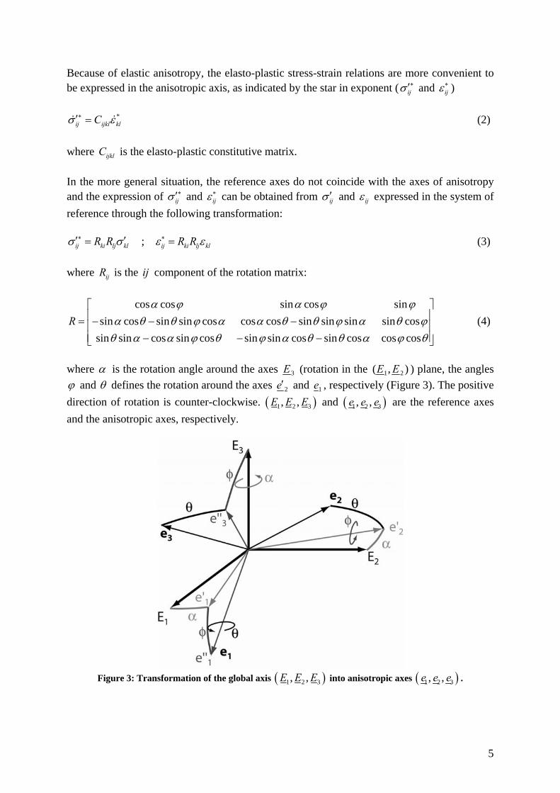
where α is the rotation angle around the axes 3E (rotation in the 1 2( , )E E ) plane, the angles ϕ and θ defines the rotation around the axes 2e′ and 1e , respectively (Figure 3). The positive direction of rotation is counter-clockwise. ( )1 2 3, ,E E E and ( )1 2 3, ,e e e are the reference axes and the anisotropic axes, respectively.

Figure 3: Transformation of the global axis ( )1 2 3, ,E E E into anisotropic axes ( )1 2 3, ,e e e .

6

At the end of each step of computation, the stress and strain obtained in the anisotropic axes ( ijσ ∗′ and ijε

∗ ) are re-transformed to be expressed in the global axes ( ijσ ′ and ijε ):

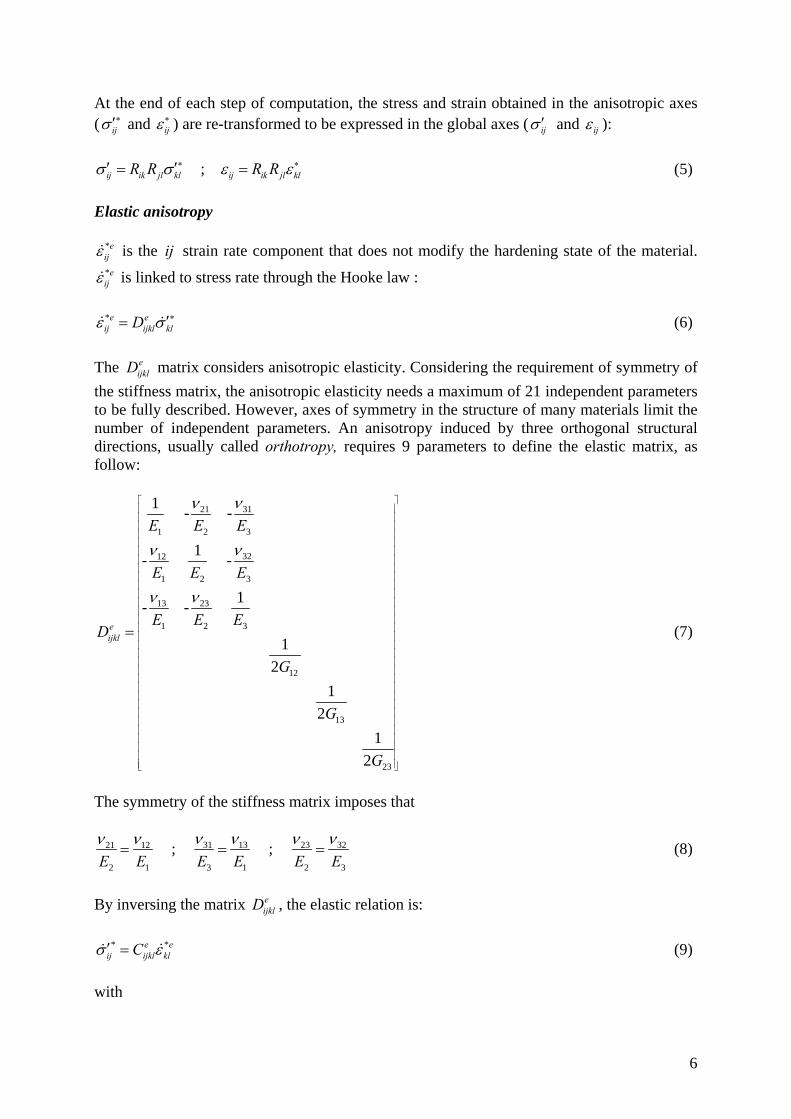
; ij ik jl kl ij ik jl klR R R Rσ σ ε ε∗ ∗′ ′= = (5) Elastic anisotropy

*eijε is the ij strain rate component that does not modify the hardening state of the material. *eijε is linked to stress rate through the Hooke law :

*e eij ijkl klDε σ ∗′= (6)

The e

ijklD matrix considers anisotropic elasticity. Considering the requirement of symmetry of the stiffness matrix, the anisotropic elasticity needs a maximum of 21 independent parameters to be fully described. However, axes of symmetry in the structure of many materials limit the number of independent parameters. An anisotropy induced by three orthogonal structural directions, usually called orthotropy, requires 9 parameters to define the elastic matrix, as follow:

3121

1 2 3

3212

1 2 3

13 23

1 2 3

12

13

23

1 - -

1- -

1- -

12

12

12

eijkl

E E E

E E E

E E ED

G

G

G

νν

νν

ν ν

⎡ ⎤⎢ ⎥⎢ ⎥⎢ ⎥⎢ ⎥⎢ ⎥⎢ ⎥⎢ ⎥⎢ ⎥⎢ ⎥⎢ ⎥⎢ ⎥⎢ ⎥⎢ ⎥⎢ ⎥⎢ ⎥⎢ ⎥⎢ ⎥⎢ ⎥⎢ ⎥⎢ ⎥⎢ ⎥⎢ ⎥⎢ ⎥⎢ ⎥⎢ ⎥⎢ ⎥⎢ ⎥⎢ ⎥⎢ ⎥⎢ ⎥⎢ ⎥⎣ ⎦

= (7)

The symmetry of the stiffness matrix imposes that

31 13 23 3221 12

2 1 3 1 2 3

; ; E E E E E E

ν ν ν νν ν= = = (8)

By inversing the matrix e

ijklD , the elastic relation is:

* *e eij ijkl klCσ ε′ = (9)

with

7

23 32 21 31 23 21 32 31

2 3 2 3 2 3

12 13 32 13 31 32 31 12

1 3 1 3 1 3

13 23 12 23 21 13 21 12

1 2 1 2 1 2

12

13

23

1det det det

1det det det

1det det det

22

2

eijkl

E E E E E E

E E E E E EC

E E E E E EG

GG

ν ν ν ν ν ν ν ν

ν ν ν ν ν ν ν ν

ν ν ν ν ν ν ν ν

⎡ ⎤⎢ ⎥⎢ ⎥⎢ ⎥⎢ ⎥⎢ ⎥⎢ ⎥⎢ ⎥⎢⎢⎢⎢⎢⎢⎢⎢⎢⎢⎢⎢⎢⎢⎢⎢⎣ ⎦

− + +

+ − +

+ + −=

⎥⎥⎥⎥⎥⎥⎥⎥⎥⎥⎥⎥⎥⎥⎥⎥

(10)

with

31 13 21 12 32 23 31 12 23

1 2 3

1 2detE E E

ν ν ν ν ν ν ν ν ν− − − −= (11)

Sedimentary rocks show usually a more limited form of anisotropy. The behaviour is isotropic in the plane of bedding and the unique direction of anisotropy is perpendicular to bedding. The properties of such materials are independent of rotation about an axis of symmetry normal to the bedding plane (Graham and Houlsby, 1982). This type of elastic anisotropy, called transverse isotropy or cross-anisotropy, requires 5 independent parameters and is a particular case of Equations (7) and (10) for which

( )

12 //,//

13 23 //,

13 23 //,

//12 //,//

//,//

1 2 //

3

2 1

G G GEG G

E E EE Eν ν

ν ν ν

ν

⊥

⊥

⊥

⎧⎪ =⎪⎪ =⎪⎪ = =⎨⎪ = =⎪⎪

= =⎪+⎪⎩

= =

(12)

where the subscripts // and ⊥ indicates, respectively, the direction parallel to bedding (directions 1 and 2) and perpendicular to bedding (direction 3). Plasticity The Drucker-Prager plastic yield limit, flow rule and consistency condition are expressed in the anisotropic axis (stress and strain components are expressed with a star exponent). This way of proceed aims at keeping the elastic matrix (needed in the development of the consistency condition) as simple as possible. The limit between the elastic and the plastic domain is represented by a yield surface in the principal stress space. This surface corresponds to the Drucker-Prager yield surface f (Drucker and Prager, 1952):

8

ˆ3 0

tancf II m Iσ σ φ

⎛ ⎞= − − =⎜ ⎟

⎝ ⎠ (13)

with

( )2sin

3 3 sinm φ

φ=

− (14)

Iσ and ˆIIσ are the first stress tensor invariant and the second deviatoric stress tensor invariant, respectively:

iiIσ σ ∗′= (15)

ˆ1 ˆ ˆ ˆ ; 2 3ij ij ij ij ij

III σσ σ σ σ σ δ∗ ∗ ∗ ∗′ ′ ′ ′= = − (16)

In Equation (13), the linear coefficient m between the first and the second stress invariant being independent of the third invariant (or alternatively, the Lode angle), the plastic surface is a cone in the principal stress space. The trace of this plasticity surface on the Π plane (deviatoric plane) is a circle (Figure 4).

Figure 4: Yield surface of the Drucker-Prager criterion in the deviatoric plane. Comparison with the Mohr-Coulomb yield surface.

The material cohesion depends on the angle between major principal stress and the normal to the bedding plane. Three cohesion values are defined, for major principal stress parallel (

10σα = ° ), perpendicular (

190σα = ° ) and with an angle of 45° (

145σα = ° ) with respect to the

normal to bedding plane. Between those values, cohesion varies linearly with1σ

α . The mathematical expression of the cohesion is as follows (Figure 5):

9

( )1 1

45 0 45 00 45max ; 45

45 45 c c c cc c cσ σα α° ° ° °

° °

⎡ − − ⎤⎛ ⎞ ⎛ ⎞= + − ° +⎜ ⎟ ⎜ ⎟⎢ ⎥° °⎝ ⎠ ⎝ ⎠⎣ ⎦ (17)

with

1σα being the angle between the normal to the bedding plane n and the major principal

stress 1σ :

1

1

1

.arccos nnσσασ′⎛ ⎞= ⎜ ⎟′⎝ ⎠

(18)

Figure 5: Schematic view of the cohesion evolution as a function of the angle between the normal vector to

bedding plane and the direction of major principal stress. A general non-associated plasticity framework is considered:

p Pij

ij

gε λσ

∗∗

∂=

′∂ (19)

with the plastic potential g defined as:

ˆ 0g II m Iσ σ′= + = (20) with

( )2sin

3 3 sinm ψ

ψ′ =

− (21)

where ψ is the dilatancy angle. When ψ φ= , ij ij

f gσ σ∗ ∗

∂ ∂=

′ ′∂ ∂ and the flow rule is associated.

The plastic multiplier pλ is obtained from the consistency condition which states that during plastic flow, the stress state stays on the limit surface:

0ijij

f fdf σ κσ κ

∗∗

∂ ∂′= + =′∂ ∂

(22)

10

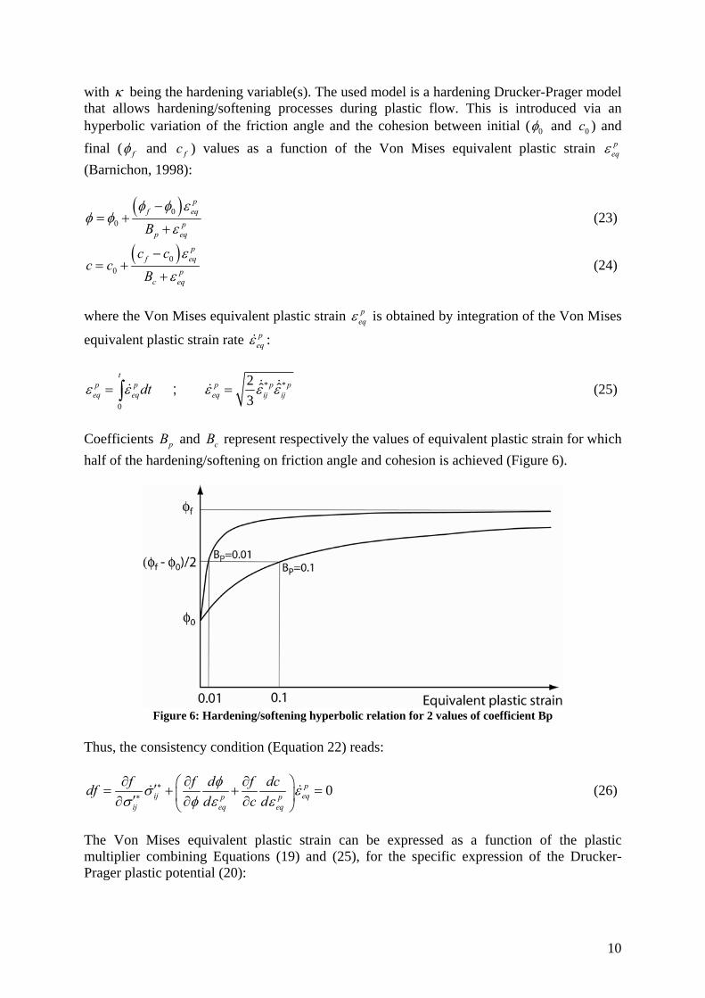
with κ being the hardening variable(s). The used model is a hardening Drucker-Prager model that allows hardening/softening processes during plastic flow. This is introduced via an hyperbolic variation of the friction angle and the cohesion between initial ( 0φ and 0c ) and final ( fφ and fc ) values as a function of the Von Mises equivalent plastic strain p

eqε (Barnichon, 1998):

( )00

pf eq

pp eqB

φ φ εφ φ

ε−

= ++

(23)

( )00

pf eq

pc eq

c cc c

Bε

ε−

= ++

(24)

where the Von Mises equivalent plastic strain p

eqε is obtained by integration of the Von Mises

equivalent plastic strain rate peqε :

* *

0

2 ˆ ˆ3

tp p p p p

eq eq eq ij ijdtε ε ε ε ε= =∫ ; (25)

Coefficients pB and cB represent respectively the values of equivalent plastic strain for which half of the hardening/softening on friction angle and cohesion is achieved (Figure 6).

Figure 6: Hardening/softening hyperbolic relation for 2 values of coefficient Bp

Thus, the consistency condition (Equation 22) reads:

0pij eqp p

ij eq eq

f f d f dcdfd c dφσ ε

σ φ ε ε∗

∗

∂ ∂ ∂⎛ ⎞′= + + =⎜ ⎟′∂ ∂ ∂⎝ ⎠ (26)

The Von Mises equivalent plastic strain can be expressed as a function of the plastic multiplier combining Equations (19) and (25), for the specific expression of the Drucker-Prager plastic potential (20):

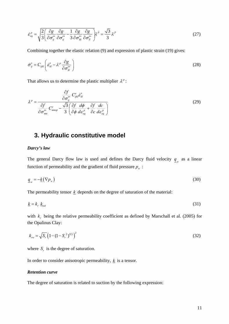
11

2 1 33 3 3

p P Peq

ij ij kk ll

g g g gε λ λσ σ σ σ∗ ∗ ∗ ∗

∂ ∂ ∂ ∂⎛ ⎞= − =⎜ ⎟′ ′ ′ ′∂ ∂ ∂ ∂⎝ ⎠ (27)

Combining together the elastic relation (9) and expression of plastic strain (19) gives:

pij ijkl kl

kl

gCσ ε λσ

∗ ∗∗

∂⎛ ⎞= −⎜ ⎟′∂⎝ ⎠ (28)

That allows us to determine the plastic multiplier pλ :

33

eijkl kl

ijp

emnop p p

mn eq eq

f C

f f d f dcCd c d

εσ

λφ

σ φ ε ε

∗∗

∗

∂′∂

=∂ ∂ ∂⎛ ⎞− +⎜ ⎟′∂ ∂ ∂⎝ ⎠

(29)

3. Hydraulic constitutive model Darcy’s law The general Darcy flow law is used and defines the Darcy fluid velocity

wq as a linear

function of permeability and the gradient of fluid pressure wp :

( )wwq k p= − ∇ (30) The permeability tensor k depends on the degree of saturation of the material:

r satk k k= (31) with rk being the relative permeability coefficient as defined by Marschall et al. (2005) for the Opalinus Clay:

( )22 0.51 (1 )rw r rk S S= − − (32) where rS is the degree of saturation. In order to consider anisotropic permeability, k is a tensor. Retention curve The degree of saturation is related to suction by the following expression:

12

1(1 )2 2

11

CSR CSRw

rpS

CSR

− −⎛ ⎞−⎛ ⎞= +⎜ ⎟⎜ ⎟⎜ ⎟⎝ ⎠⎝ ⎠

(33)

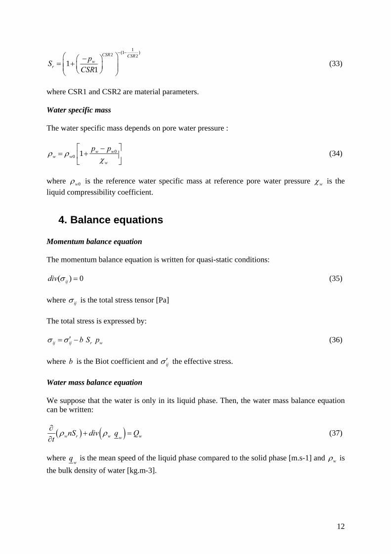
where CSR1 and CSR2 are material parameters. Water specific mass The water specific mass depends on pore water pressure :

00 1 w w

w ww

p pρ ρχ

⎡ ⎤−= +⎢ ⎥

⎣ ⎦ (34)

where 0wρ is the reference water specific mass at reference pore water pressure wχ is the liquid compressibility coefficient.

4. Balance equations Momentum balance equation The momentum balance equation is written for quasi-static conditions:

( ) 0ijdiv σ = (35) where ijσ is the total stress tensor [Pa] The total stress is expressed by:

ij ij r wb S pσ σ ′= − (36) where b is the Biot coefficient and ijσ ′ the effective stress. Water mass balance equation We suppose that the water is only in its liquid phase. Then, the water mass balance equation can be written:

( ) ( ) w r w wwnS div q Q

tρ ρ∂

+ =∂

(37)

where

wq is the mean speed of the liquid phase compared to the solid phase [m.s-1] and wρ is

the bulk density of water [kg.m-3].

13

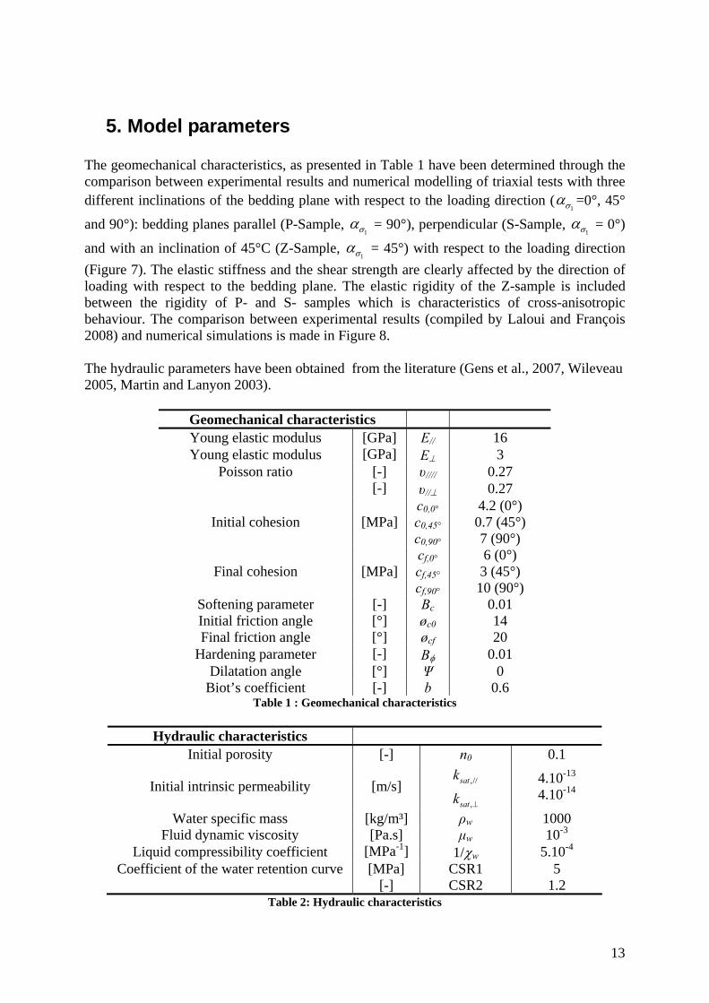
5. Model parameters The geomechanical characteristics, as presented in Table 1 have been determined through the comparison between experimental results and numerical modelling of triaxial tests with three different inclinations of the bedding plane with respect to the loading direction (

1σα =0°, 45°

and 90°): bedding planes parallel (P-Sample, 1σ

α = 90°), perpendicular (S-Sample, 1σ

α = 0°)

and with an inclination of 45°C (Z-Sample, 1σ

α = 45°) with respect to the loading direction (Figure 7). The elastic stiffness and the shear strength are clearly affected by the direction of loading with respect to the bedding plane. The elastic rigidity of the Z-sample is included between the rigidity of P- and S- samples which is characteristics of cross-anisotropic behaviour. The comparison between experimental results (compiled by Laloui and François 2008) and numerical simulations is made in Figure 8. The hydraulic parameters have been obtained from the literature (Gens et al., 2007, Wileveau 2005, Martin and Lanyon 2003).

Geomechanical characteristics Young elastic modulus [GPa] E// 16 Young elastic modulus [GPa] E⊥ 3

Poisson ratio [-] υ//// 0.27 [-] υ//⊥ 0.27

Initial cohesion [MPa] c0,0° c0,45° c0,90°

4.2 (0°) 0.7 (45°) 7 (90°)

Final cohesion [MPa] cf,0° cf,45° cf,90°

6 (0°) 3 (45°) 10 (90°)

Softening parameter [-] Bc 0.01 Initial friction angle [°] øc0 14 Final friction angle [°] øcf 20

Hardening parameter [-] Bφ 0.01 Dilatation angle [°] Ψ 0

Biot’s coefficient [-] b 0.6 Table 1 : Geomechanical characteristics

Hydraulic characteristics

Initial porosity [-] n0 0.1

Initial intrinsic permeability [m/s] ,//satk

,satk ⊥

4.10-13

4.10-14

Water specific mass [kg/m³] ρw 1000 Fluid dynamic viscosity [Pa.s] µw 10-3

Liquid compressibility coefficient [MPa-1] 1/χw 5.10-4 Coefficient of the water retention curve [MPa] CSR1 5

[-] CSR2 1.2 Table 2: Hydraulic characteristics

14

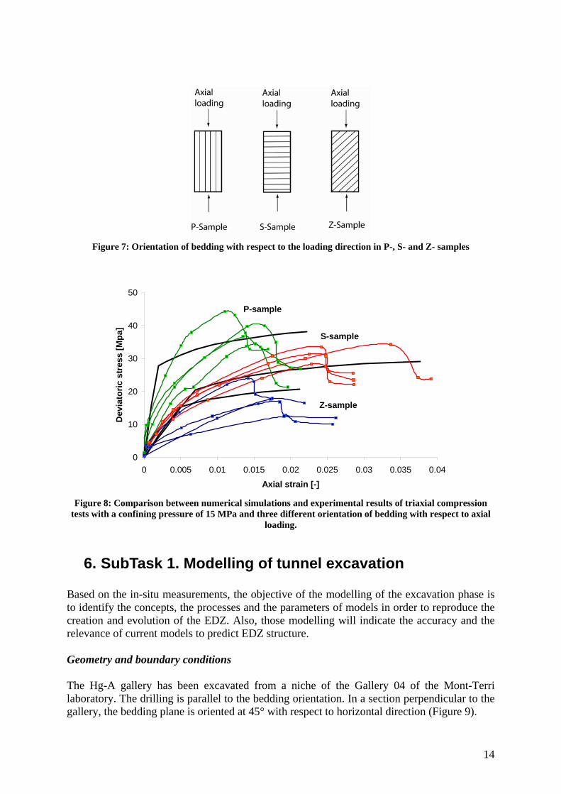
Figure 7: Orientation of bedding with respect to the loading direction in P-, S- and Z- samples

0

10

20

30

40

50

0 0.005 0.01 0.015 0.02 0.025 0.03 0.035 0.04

Axial strain [-]

Dev

iato

ric s

tres

s [M

pa]

P-sample

S-sample

Z-sample

Figure 8: Comparison between numerical simulations and experimental results of triaxial compression

tests with a confining pressure of 15 MPa and three different orientation of bedding with respect to axial loading.

6. SubTask 1. Modelling of tunnel excavation Based on the in-situ measurements, the objective of the modelling of the excavation phase is to identify the concepts, the processes and the parameters of models in order to reproduce the creation and evolution of the EDZ. Also, those modelling will indicate the accuracy and the relevance of current models to predict EDZ structure. Geometry and boundary conditions The Hg-A gallery has been excavated from a niche of the Gallery 04 of the Mont-Terri laboratory. The drilling is parallel to the bedding orientation. In a section perpendicular to the gallery, the bedding plane is oriented at 45° with respect to horizontal direction (Figure 9).

15

Figure 9: Schematic view of the orientation of the Hg-A gallery with respect to bedding plane.

The problem has been considered as a 2D plane strain problem, considering a perpendicular section in the middle of the gallery. A 40 m wide square domain has been considered. The initial stress is anisotropic: σZ = 8 MPa (vertical stress), σX = 3 MPa (horizontal radial stress) and σY = 1.3 MPa (horizontal axial stress). The initial pore water pressure has been fixed to 0.9 MPa. In term of mechanical conditions, the external boundaries are kinematically constrained (no displacement) (Figure 10). The internal boundary (at the gallery wall) is stress controlled. To simulate the excavation phase, the total stress at the gallery wall is decreased from the initial anisotropic stress to 0 MPa within one day (86400 s). The pore water pressure is maintained constant at 0.9 MPa on the external boundaries while the pore water pressure at the gallery wall is reduced from 0.9 MPa to 0 MPa in 1 day. Afterward, to reproduce gallery ventilation, pore water pressure is linearly decreased from 0 to -24 MPa in 7 days and then a constant pressure of -24 MPa is maintained. Seepage elements are considered on the gallery wall. That condition allows flow of water from the ground to the gallery (if the pore pressure of the ground is higher than the imposed pore pressure at the gallery wall) but restrict flow of water from the gallery to the ground.

Figure 10: Boundary conditions of the 2D plane strain model.

16

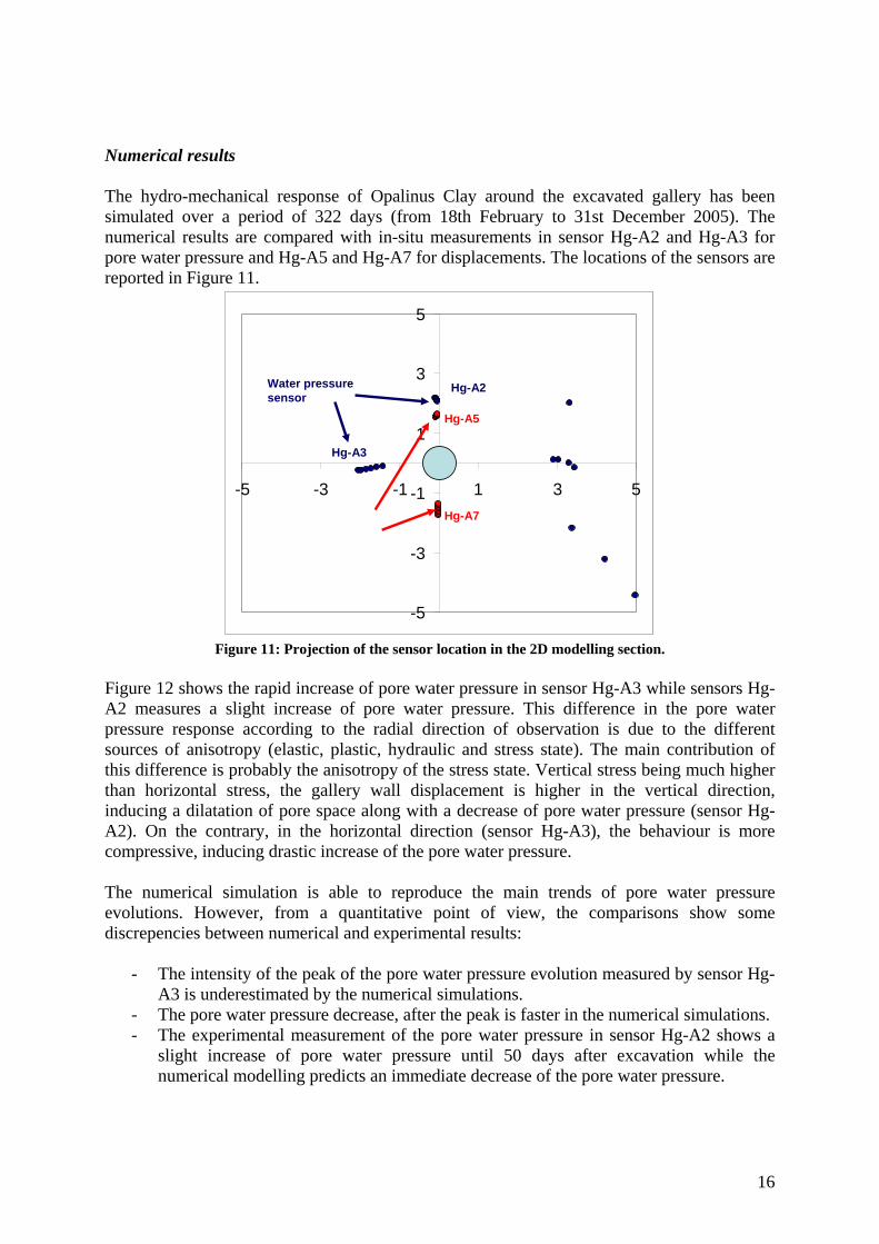
Numerical results The hydro-mechanical response of Opalinus Clay around the excavated gallery has been simulated over a period of 322 days (from 18th February to 31st December 2005). The numerical results are compared with in-situ measurements in sensor Hg-A2 and Hg-A3 for pore water pressure and Hg-A5 and Hg-A7 for displacements. The locations of the sensors are reported in Figure 11.

-5

-3

-1

1

3

5

-5 -3 -1 1 3 5

Hg-A3

Hg-A2

Hg-A5

Hg-A7

Water pressure sensor

-5

-3

-1

1

3

5

-5 -3 -1 1 3 5

-5

-3

-1

1

3

5

-5 -3 -1 1 3 5

Hg-A3

Hg-A2

Hg-A5

Hg-A7

Water pressure sensor

Figure 11: Projection of the sensor location in the 2D modelling section.

Figure 12 shows the rapid increase of pore water pressure in sensor Hg-A3 while sensors Hg-A2 measures a slight increase of pore water pressure. This difference in the pore water pressure response according to the radial direction of observation is due to the different sources of anisotropy (elastic, plastic, hydraulic and stress state). The main contribution of this difference is probably the anisotropy of the stress state. Vertical stress being much higher than horizontal stress, the gallery wall displacement is higher in the vertical direction, inducing a dilatation of pore space along with a decrease of pore water pressure (sensor Hg-A2). On the contrary, in the horizontal direction (sensor Hg-A3), the behaviour is more compressive, inducing drastic increase of the pore water pressure. The numerical simulation is able to reproduce the main trends of pore water pressure evolutions. However, from a quantitative point of view, the comparisons show some discrepencies between numerical and experimental results:

- The intensity of the peak of the pore water pressure evolution measured by sensor Hg-A3 is underestimated by the numerical simulations.

- The pore water pressure decrease, after the peak is faster in the numerical simulations. - The experimental measurement of the pore water pressure in sensor Hg-A2 shows a

slight increase of pore water pressure until 50 days after excavation while the numerical modelling predicts an immediate decrease of the pore water pressure.

17

Figure 13 compares total displacement of sensor Hg-A5 (1m above the gallery) and Hg-A7 (1m below the excavation). After an immediate displacement 0.5 mm, the displacements continue to increase due to consolidation processes. The immediate response is well reproduced by the model. However, the subsequent evolution of the displacements is slightly under-estimated by the model. The modelled displacement in sensor Hg-A5 and Hg-A7 are equal but opposite in sign. This is because those sensors are located in symmetric orientations (-90° and +90°) with respect to the different anisotropic directions: 45° and 135° for elastic modulus, cohesion and water permeability and 0° and 90° for in-situ stress.

0.0E+00

5.0E+05

1.0E+06

1.5E+06

2.0E+06

2.5E+06

0 50 100 150 200 250 300 350Time (Days)

Wat

er p

ress

ure

(Pa)

B-A03PE1 (simu)B-A03PE2 (simu)B-A03PE3 (simu)B-A02PE2 (simu)B-A03PE1 (exp.)B-A03PE2 (exp.)B-A03PE3 (exp.)B-A02PE2 (exp.)

Figure 12: Comparison between numerical simulation and experimental results of the time evolution of

the pore water pressure in sensor Hg-A02 and Hg-A03.

-2.00E-03

-1.50E-03

-1.00E-03

-5.00E-04

0.00E+00

5.00E-04

1.00E-03

1.50E-03

2.00E-03

0 50 100 150 200 250 300 350

Time (Days)

Dis

plac

emen

t (m

)

B-A05DE04 (simu)B-A07DE04 (simu)B-A05DE04 (exp.)B-A07DE04 (exp.)

Figure 13: Comparison between numerical simulation and experimental results of the time evolution of

the total displacement in sensor Hg-A05 and Hg-A07.

18

Even if the general trend of numerical results is in good agreement with experimental measurements, the quantitative differences can be related to two aspects:

- The model parameters of the mechanical model have been determined from independent triaxial tests. So, the numerical simulations consist in blind prediction and not in an optimization procedure.

- The 3D complex geometry of the system has been simplified into a 2D plane strain problem. The effect of the impervious liner installed in the 6 first meters of the gallery has not been considered. However, this liner has a mechanical and hydraulic effect on the global hydro-mechanical response. Also, the 2D simulation does not allow the consideration of the excavation step. Finally, all the sensors that are located in a 3D space have been projected in the 2D modelled plane. So, the longitudinal location of the sensors has not been considered in the simulation.

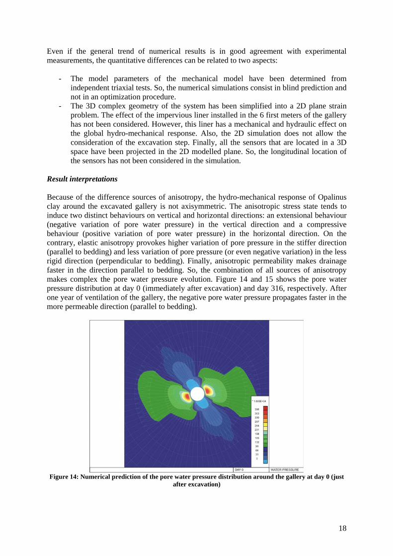
Result interpretations Because of the difference sources of anisotropy, the hydro-mechanical response of Opalinus clay around the excavated gallery is not axisymmetric. The anisotropic stress state tends to induce two distinct behaviours on vertical and horizontal directions: an extensional behaviour (negative variation of pore water pressure) in the vertical direction and a compressive behaviour (positive variation of pore water pressure) in the horizontal direction. On the contrary, elastic anisotropy provokes higher variation of pore pressure in the stiffer direction (parallel to bedding) and less variation of pore pressure (or even negative variation) in the less rigid direction (perpendicular to bedding). Finally, anisotropic permeability makes drainage faster in the direction parallel to bedding. So, the combination of all sources of anisotropy makes complex the pore water pressure evolution. Figure 14 and 15 shows the pore water pressure distribution at day 0 (immediately after excavation) and day 316, respectively. After one year of ventilation of the gallery, the negative pore water pressure propagates faster in the more permeable direction (parallel to bedding).

Figure 14: Numerical prediction of the pore water pressure distribution around the gallery at day 0 (just

after excavation)

19

Figure 15: Numerical prediction of the pore water pressure distribution around the gallery at day 316

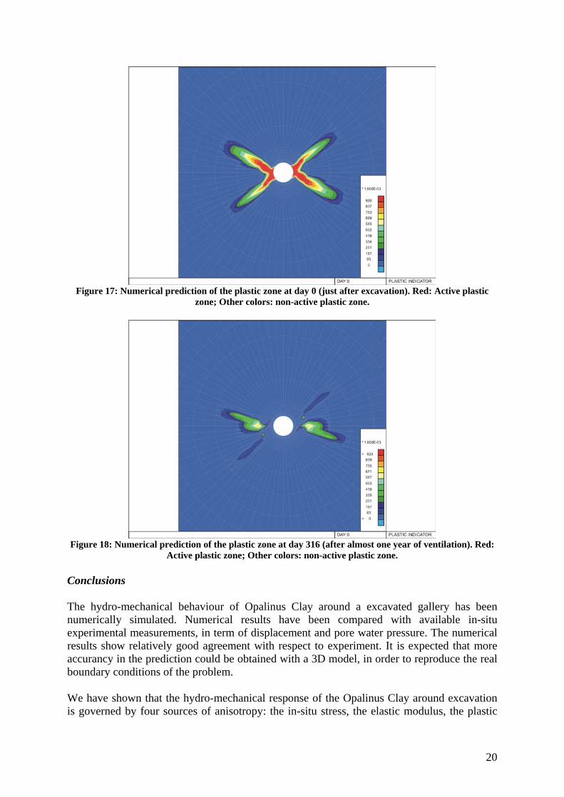
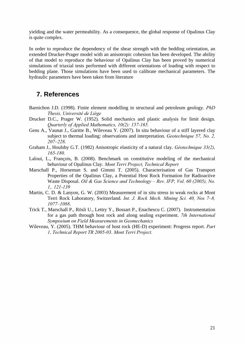
(after almost one year of ventilation) Figure 16 shows the deformed mesh one year after the excavation. The minimum and maximum displacements occur at 30° and 120° with respect to x axis, respectively. At short term after excavation, plastic zone develops in preferential directions at 30° and 150° with respect to x-axis (Figure 17). Those directions correspond probably to the zone in which maximum shear stresses are concentrated. At the end of the simulation, the negative pore water pressure (suction) induced by the gallery ventilation provokes an increase in strength. As a consequence, the plastic processes are suppressed and the behaviour is elastic (Figure 18).

Figure 16: Numerical prediction of the deformation of the gallery at day 316 (after almost one year of

ventilation). Maximum displacement: 2.05mm.

20

Figure 17: Numerical prediction of the plastic zone at day 0 (just after excavation). Red: Active plastic

zone; Other colors: non-active plastic zone.

Figure 18: Numerical prediction of the plastic zone at day 316 (after almost one year of ventilation). Red:

Active plastic zone; Other colors: non-active plastic zone. Conclusions The hydro-mechanical behaviour of Opalinus Clay around a excavated gallery has been numerically simulated. Numerical results have been compared with available in-situ experimental measurements, in term of displacement and pore water pressure. The numerical results show relatively good agreement with respect to experiment. It is expected that more accurancy in the prediction could be obtained with a 3D model, in order to reproduce the real boundary conditions of the problem. We have shown that the hydro-mechanical response of the Opalinus Clay around excavation is governed by four sources of anisotropy: the in-situ stress, the elastic modulus, the plastic

21

yielding and the water permeability. As a consequence, the global response of Opalinus Clay is quite complex. In order to reproduce the dependency of the shear strength with the bedding orientation, an extended Drucker-Prager model with an anisotropic cohesion has been developed. The ability of that model to reproduce the behaviour of Opalinus Clay has been proved by numerical simulations of triaxial tests performed with different orientations of loading with respect to bedding plane. Those simulations have been used to calibrate mechanical parameters. The hydraulic parameters have been taken from literature

7. References Barnichon J.D. (1998). Finite element modelling in structural and petroleum geology. PhD

Thesis, Université de Liège Drucker D.C., Prager W. (1952). Solid mechanics and plastic analysis for limit design.

Quarterly of Applied Mathematics, 10(2): 157-165. Gens A., Vaunat J., Garitte B., Wileveau Y. (2007). In situ behaviour of a stiff layered clay

subject to thermal loading: observations and interpretation. Geotechnique 57, No. 2, 207–228.

Graham J., Houlsby G.T. (1982) Anisotropic elasticity of a natural clay. Géotechnique 33(2), 165-180.

Laloui, L., François, B. (2008). Benchmark on constitutive modeling of the mechanical behaviour of Opalinus Clay. Mont Terri Project, Technical Report

Marschall P., Horseman S. and Gimmi T. (2005). Characterisation of Gas Transport Properties of the Opalinus Clay, a Potential Host Rock Formation for Radioactive Waste Disposal. Oil & Gas Science and Technology – Rev. IFP, Vol. 60 (2005), No. 1,. 121-139

Martin, C. D. & Lanyon, G. W. (2003) Measurement of in situ stress in weak rocks at Mont Terri Rock Laboratory, Switzerland. Int. J. Rock Mech. Mining Sci. 40, Nos 7–8, 1077–1088.

Trick T., Marschall P., Rösli U., Lettry Y., Bossart P., Enachescu C. (2007). Instrumentation for a gas path through host rock and along sealing experiment. 7th International Symposium on Field Measurements in Geomechanics

Wileveau, Y. (2005). THM behaviour of host rock (HE-D) experiment: Progress report. Part 1, Technical Report TR 2005-03. Mont Terri Project.