MODELLING OF A LARGE BOREHOLE HEAT

EXCHANGERS INSTALLATION IN SWEDEN

Master Thesis KTH Royal Institute of Technology Department of Energy Technology

Division of Applied Thermodynamics and Refrigeration

Mauro Biancucci

2

3

ABSTRACT

In the last years the ground source heat pump (GSHP) systems achieved resounding success in the

Swedish market thanks to a growing technological and economic development. The increasing

demand of cooling energy, in commercial and industrial fields, encouraged the growth of a larger

market of geothermal systems with multiple boreholes.

This technology represents an important component in the strategy to reduce the energy consumption

and limit the greenhouse gas emissions in order to reach Europe’s climate and energy targets.

The project has been conducted from March 2015 to September 2015 at the Department of Energy

Technology of KTH Royal Institute of Technology.

During this exchange period, a large scale installation of 130 boreholes with uneven pattern placed in

Stockholm has been simulated. In this context, different study cases have been analysed: a single

borehole, a couple of boreholes, a group of boreholes and, at the end, the whole installation divided in

different thermal zones.

The first task was to check the validity of the code against relevant publications and the possible

limitations of the analytical model based on the Finite Line Source (FLS).

The aim of the thesis is to simulate the thermal process of this uneven boreholes field and predict the

fluid temperature’s drift under different conditions in the short-term and in the long-term. Moreover

the effect of the imbalance between cooling and heating demand has been examined with special

attention to the starting simulation month.

As a result, the differences in the g-function values observed between the proposed method and the

pre-processor increase directly with the increasing number of the boreholes.

At the end of the analysis, the decrease of the energy flow’s imbalance turns out to be effective to the

improvement of the system’s performance, decreasing the maximum reached fluid temperature.

4

5

TABLE OF CONTESTS

ABSTRACT ...................................................................................................................... 3

TABLE OF CONTESTS ...................................................................................................... 5

1. INTRODUCTION ...................................................................................................... 8

1.1 BACKGROUND ................................................................................................................................ 8

1.2 TECHNOLOGY DESCRIPTION ........................................................................................................... 9

1.3 AIM OF THE STUDY ....................................................................................................................... 12

2. THEORETICAL BACKGROUND ............................................................................... 16

2.1 MODEL OF A SINGLE BOREHOLE HEAT EXCHANGER ....................................................................... 16

2.2 STUDY OF THE G-FUNCTION ......................................................................................................... 18

2.3 DIFFERENT WORK MODELLING INSTALLATIONS .............................................................................. 24

3. DESCRIPTION OF THE FRESCATI INSTALLATION .................................................... 30

4. METHODOLOGY .................................................................................................... 34

4.1 APPROACH CARRIED OUT IN THE STUDY ........................................................................................ 34

4.2 NEW BHES ARRANGEMENT ........................................................................................................... 39

4.3 ASSUMPTIONS MADE .................................................................................................................... 41

4.4 LOAD PROFILES FOR THE INSTALLATION IN HOURLY AND MONTHLY CASES ...................................... 41

5. RESULTS ............................................................................................................... 46

5.1 G-FUNCTION FOR THE BOREHOLE FIELD IN FRESCATI ................................................................... 46

5.2 ABOUT THE SHORT TERM SIMULATION WITH HOURLY HEAT LOAD PROFILE ...................................... 48

5.2.1 Starting point in October .................................................................................................... 50

5.2.2 Balanced load profile ......................................................................................................... 51

5.3 ABOUT THE LONG TERM SIMULATION WITH MONTHLY HEAT LOAD PROFILE ..................................... 53

6

5.3.1 Starting point in October .................................................................................................... 56

5.3.2 Balanced load profile ......................................................................................................... 57

7. CONCLUSIONS .......................................................................................................... 62

7

8

1. INTRODUCTION

1.1 Background

One of the most innovative and attractive way to supply heating and cooling demand, in residential

and commercial buildings, is represented by Ground Source Heat Pump (GSHP) systems.

In the last years the use of this technology spread gradually across the world, since it is suitable to

decrease operational costs of energy supply system and to reduce as the use of fossil energy sources as

the dependence on the imported fuels.

It must be said that the fossil fuels represent the major competitor with less initial investment costs,

but then the decrease of oil and gas supplies and their increasing price make the ground an even more

economically viable alternative source of energy.

Geothermal systems have got success in Sweden, where the geothermal energy is dominated by low

temperature, shallow geothermal systems and direct use. Indeed GSHP stands for one of the most

installed systems, which supply energy demand approximately to 20% of the Swedish buildings,

making Sweden one of the first leading countries within this technology, not only in terms of annual

energy use but also in terms of installed capacity [1].

According to the study made by Andersson and Bjelm in 2013, the geothermal energy is the 3rd largest

renewable energy source used in this country, thanks to an incredible growth of the GSHP systems

related to their high energy efficiency potential [2].

Nowadays the geothermal heat pump’s market represents the predominant market in Sweden, playing

a significant role in Sweden’s dwellings to achieve a sustainable development.

Starting from the end of the 1970s, after the oil crisis, different solutions were taken in order to reduce

the use of oil for heating. In the early 1980s the use of heat pumps, coupled with ground as heat

source, gained suddenly popularity in Sweden and by 1985 a large number of installations were

recorded.

9

At that time the poor reputation about available technology and the withdrawal of subsidies for heat

pump technologies caused a significantly deadlock of heat pump market in the late 1980s and early

1900s. Indeed the low quality and poorly performing heat pumps led to a negative public view of the

technology’s reliability.

The real growth of the Swedish GHP market arrived in 1995 thanks to the strong support measures of

the Swedish State and to the programme sponsored by the Swedish Agency for Economic and

Regional Growth (NUTEK) [3].

With the aim of developing reliable and improved heat pumps for residential buildings, this

programme increased the sales of geothermal heat pumps. At the beginning of 2000s the total number

of installations reached the peak around 200,000 units, covering about 90% of the residential market

[4].

The data from the Swedish Heat Pump Association until 2015 show that about 500,000 GSHP

systems are installed in Sweden, of which in the last five years around 25,000 GSHP units have been

installed per annum, especially for small power sizes. The prevalent variants of GSHPs are small

systems which supply individual residential houses with an installed mean power by around 10 kW

[5].

In addition to the consolidated residential market, during last few years a new market for larger

shallow geothermal energy systems is rapidly enhancing due to increasing interest of cooling in the

commercial and industrial sector [6].

1.2 Technology description

First of all, let us make clearer what a heat pump system consist on. Heat pump plays an important

role for space and water heating as well as for cooling purpose in the building and industry market.

Today more than one million of heat pump units are installed in Sweden, mainly in residential

dwellings [7].

10

The heat pumps use renewable energy sources from ground, air and water: everyone gets various

advantages as well as disadvantages and has a strong influence on the heat pump capacity. Renewable

sources of heating and cooling can also be cheaper than fossil alternatives in the long-term operation

and contribute to significantly energy savings.

They provide energy from a heat source to a heat sink through auxiliary energy use, as electricity or

gas, moving thermal energy in opposite way to the natural direction; from low to high temperatures.

Then the extracted heat from the ambient (heat source) is supposed to be supplied at higher

temperature to the building (heat sink) using a compressor. Furthermore they can provide cooling

energy by operating in reverse mode.

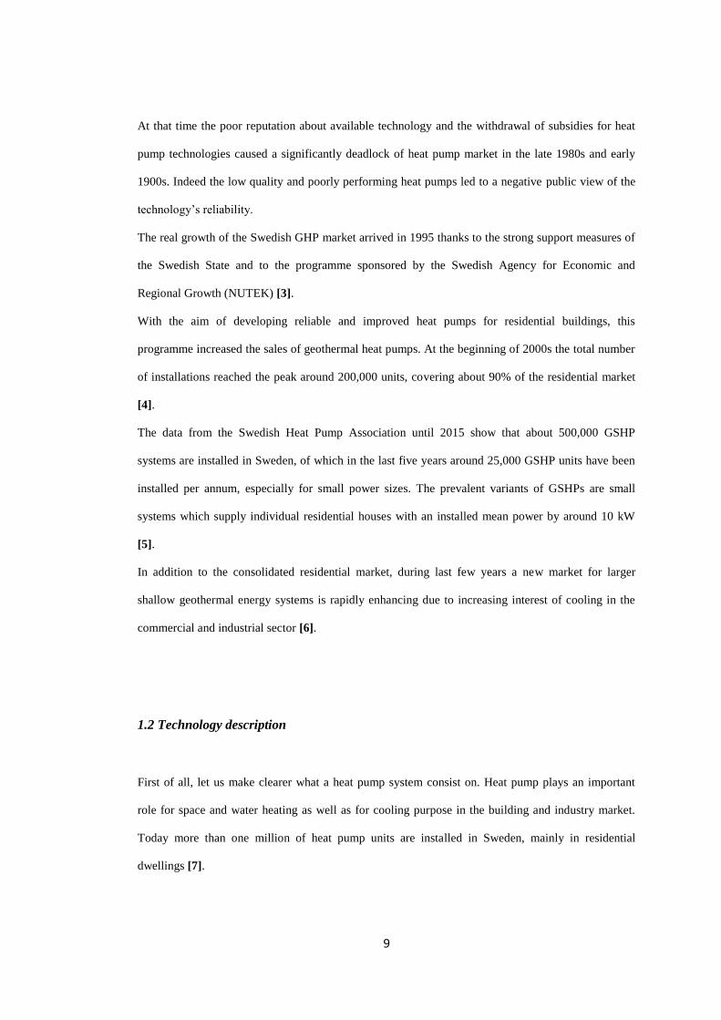
This technology relies on a vapour compression cycle, with two simple principles: evaporation and

compression. The cycle includes two heat exchangers, one compressor and one expansive valve in

order to carry heat from one space to another one. Afterwards the energy is usually supplied via

radiators, floor heating system or fan coil units.

Figure 1.1: Vapour compression cycle for a Ground Source Heat Pump system

The efficiency of a heat pump unit is described by the Coefficient of Performance (COP) in the

heating mode and by the Energy Efficiency Ratio (EER) in the cooling mode, which are the ratio of

the output energy divided by the input energy. Heat Pumps can reach efficiency by 3 or 5, which

means that one unit of electricity is transformed into three or five units of heat (in the case of heating

mode).

11

In order to fulfil the heating and cooling demand, Geothermal Heat Pumps (GHPs) are one of the most

widely used technologies in the world, since geothermal heat is an inexhaustible source of energy.

These systems could be divided in two main groups depending on the temperature level of heat source

they reach.

A great amount of heat could be reached up to depths of around 5000 m by deep geothermal systems,

which employ heat at high temperatures to generate electricity or for direct heat use applications.

Furthermore we could obtain greater efficiency by using cascade methods, which employ the waste

energy from electricity generation. Instead shallow geothermal systems, working at depths less than

300 m, use heat at lower temperature in order to supply the heating and cooling demands [4].

The use of deep geothermal energy systems is limited in Sweden and only one plant is in operation.

Since this country is dominated by low temperature, the market of shallow geothermal energy systems

has a growing trend [5].

Depending upon the type and availability of land and the possibility of drilling economically a water

well, we can divide the GHPs in two different types: groundwater systems and ground-coupled

systems.

The first one is an open loop system, which uses ground water or lake water directly in heat

exchanger. Then, depending upon the local laws, it is discharged into another well, into a stream or

lake or more over onto the ground.

Figure 1.2: Open loop heat pump systems (source: Geo-Heat Centre)

12

The second one is closed loop system, installed horizontally or vertically in the ground with a heat

circulating fluid through the plastic pipes.

Figure 1.3: Closed loop heat pump systems (source: Geo-Heat Centre)

In this kind of installation, single U-pipes are generally used in boreholes, making easier these

systems, which have a slightly higher heat transfer capacity. Furthermore, double U-pipes are

sometimes used in order to extract a greater amount of heat from the ground in winter or reject it to

the ground in summer.

The type of heat exchanger has a strong influence on the cost of the system and on the heat exchange.

The horizontal pipes, for example, are the most common type of system since their smaller installed

depth let to decrease the drilling costs. They concern the shallow layers of the ground and do not go

deeper than 1.5 m, but they need large areas of installation. Anyway they have a lower efficiency

since they are affected by variable heat loads cause of solar radiations and other weather conditions

that influences the ground temperature change in the upper layers [8].

Conversely, vertical pipes request smaller land and offer a higher efficiency, since they are affected by

smaller seasonal swing in the ground temperature. Anyway they are more expensive than horizontal

pipes. The cost of technology is influenced by the reached depths; indeed the deeper the borehole

goes, much more expensive the GSHP is [9].

1.3 Aim of the study

The technological and economical improvements make the GSHP system the main technology to

supply the energy demand in both residential dwellings and large commercial buildings.

13

The relatively constant mean temperature of the ground, compared with the ambient air, the lower

operating costs and the lower maintenance requirements, compared to ones of a conventional system,

represent the main advantages related to this technology.

Solar radiations increase the efficiency of the GSHP recharging the ground and maintaining a quite

constant temperature under about the first 13 meters deep, even throughout winter [10]. The

temperature difference, between the heat source and the heat sink, is thus lower and this leads to a

higher efficiency.

During last few years, larger heat pump installations are steadily growing in the commercial and

industrial sector, where the cooling demands find more interest. Especially for larger borehole

systems, the main point in question concerns the long-term behaviour of the borehole heat exchangers.

It is important to have a long-term balance between the heat extracted from the ground and the heat

injected to the ground: a remarkable imbalance could induce thermal anomalies.

It must be said that at northern latitudes the heating energy demand of residential buildings is not

always balanced with the cooling energy demand, as consequence this imbalance influences the

performance of these systems [11]. A long term heat extraction from the ground, during the heating

season, produces a ground and working fluid temperature changes along with a lesser capability of the

borehole field to regenerate itself. Besides, this deviation is emphasized by borehole field geometry

and by interferences between multiple neighbouring boreholes. The closer the boreholes are, the

greater the thermal interference is [12].

Recently research activities are focusing on the optimization of the borehole heat exchangers by

studying different operational modes and different geometry arrangements.

The thermal process analysis relies on the interaction between the local process and the global

process: the first one influences the heat transfer capacity of ground heat exchanger; the second one

the heat losses from the store. The thermal local process involves interaction of different boreholes,

while the thermal global process studies the heat losses of the whole studied volume.

14

The main aim of this project is to assess the performance of the borehole field and obtain an important

fluid temperature prediction for different conditions of load profile and layouts. This work intends to

realise a complete study on the thermal response of the installation.

With this purpose, the idea is to compare simulated data and real data from the committed installation

in order to test and validate the last developed theoretical models.

The project has been conducted from March 2015 to September 2015 at the Department of Energy

Technology, at KTH.

First of all, it is important to investigate the main topic and the technology used and then examine the

current results of the last approaches, also by analysing different real cases in order to understand the

theory’s limitations.

For this thesis a long work is carried out concerning a real large installation placed in Stockholm and

funded by Akademiska Hus and other companies. This project is financially supported by Swedish

Energy Agency in collaboration with Tyréns, Skanska, Stures Brunnsborrningar and Akademiska Hus

for the next three years.

It is possible to sum up the main tasks performed in these months through the following points:

Validation of the Matlab code and design of a new arrangement geometry according to the

last approach;

Simulation of the thermal process in an uneven bore field configuration;

Short-term and long-term simulations of the heat carrier fluid temperature with the given

load profile;

Prediction of the fluid temperature for a balanced load profile and with special attention to

the starting operation month.

In this project, it will be simulated the thermal behaviour of a single borehole, of a couple of

boreholes, of a small group of boreholes (manifold) and of the whole installation.

Hourly and monthly load profiles will be used in order to outline the fluid temperature profile in the

short-term (1 year) and in the long-term (20 years).

15

Several comparisons between different cases will be carried out in the dissertation. The purpose is to

understand the influence on the fluid temperature of an increasing number of boreholes, of reducing

the imbalance between heating and cooling demand and of changing the starting simulation month.

The final results will give an important contribution to check the agreement of the model with the

reality and to enhance the settled geothermal installation.

This is something interest for the people who are working on the control of the system, in order to find

new solutions to get better the performance of the system.

From the next month (October 2015), the installation will start working and supplying directly the

energy demand to the building. For this reason it will be possible to measure the real values and

compare them with the simulated results.

16

2. THEORETICAL BACKGROUND

2.1 Model of a single borehole heat exchanger

During the first months, a long work was leading in order to get as much knowledge as possible about

geothermal energy, ground heat source pumps and borehole heat exchangers, by reading several

sources such as reports, papers and scientific books.

Starting from an overview on the heat pump technology theory, the work was gradually focused on

the ground heat exchange.

The main task is to study the thermal behaviour of the bore field and predict the fluid temperature in

order to estimate the performance of the heat pumps connected to those boreholes.

First of all, it is important to explain the model of a single borehole and how it was designed. We must

bear in mind that an important part of the costs of the system is related to the heat exchanger in the

ground.

A single geothermal borehole is used to exchange heat with the surrounding ground, which acts as a

heat source during winter or a heat sink during summer. For the design of the boreholes, it needs to be

defined the heat transfer between the heating carrier fluid and the borehole and between the borehole

and the ground. In most of the approaches, the heat transfer process is simplified taking into

consideration mainly the heat conduction problem when the groundwater flow is neglected.

The amount of the heat exchanged with the ground influences the borehole wall temperature change

and the temperature of the ground surrounding.

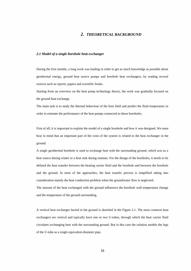
A vertical heat exchanger buried in the ground is sketched in the Figure 2.1. The most common heat

exchangers are vertical and typically have one or two U-tubes, through which the heat carrier fluid

circulates exchanging heat with the surrounding ground. But in this case the solution models the legs

of the U-tube as a single equivalent-diameter pipe.

17

Figure 2.1: Vertical borehole sketch (Source: Lamarche and Beauchamp, 2007)

The heat carrier fluid flows down to the bottom of the borehole with an inlet temperature T fi and it is

heated by the rock. Then it goes upwards and exits at the temperature Tfo, which is influenced by the

exchanger’s length.

In order to simplify the model two mean temperatures are taken into account: the fluid mean

temperature Tf (t) and the borehole wall mean temperature Tb (t). By considering a quasi-steady state

for the inner problem, the following relation (1) models the heat transfer from the ground to the inner

part of the borehole, when the heat extracted per unit length of the borehole q’(t) is negative.

𝑇𝑓(𝑡) − 𝑇𝑏(𝑡) = 𝑞′(𝑡) 𝑅′𝑏 (1)

With

𝑇𝑓(𝑡) = 𝑇𝑓𝑜 (𝑡)+𝑇𝑓𝑖 (𝑡)

2 (2)

This is the classical approach used to study the behaviour of vertical heat exchangers.

In the equation (1), R’b is the borehole resistance per unit length in the borehole. As in most of the

classic approaches, the internal part is modelled as a simple thermal resistance. It takes into

18

consideration the convention between the fluid and the borehole wall, the conduction in the tube walls

and the conduction in the grout.

Obviously the heat flux per unit length, showed in the equation, can be positive or negative in sign

depending on season. In winter, when the heat is extracted from the ground, it is negative and the fluid

temperature will be lower than the undisturbed ground temperature. In summer it will be the opposite.

Then the last term participating in the equation is the borehole wall mean temperature Tb (t) and it

depends on the thermal response of the soil.

The borehole wall temperature can be computed by the equation (3).

𝑇𝑏(𝑡) = 𝑇𝑔 + 𝑞′(𝑡) 𝑅𝑔 (3)

In the analysis of the geothermal system, some simplifications have been carried out for practical

purposes. Pure conduction and homogeneous ground properties around the boreholes are considered,

such as mean conductivity and mean diffusivity. In addition the ground is characterized by an

undisturbed temperature Tg.

Depending on the heat rate exchanged, the process affects the thermal behaviour of the ground on the

long timeframe. As a consequence, the borehole wall temperature becomes a key parameter which is

calculated defining the ground thermal resistance Rg.

2.2 Study of the g-function

Over the years, analytical and numerical solutions were carried out in order to design the vertical and

inclined boreholes, used in GCHP systems, and to investigate the long-term system performance.

Basically we could split the various approaches in two main groups: short-term performance or long-

term performance.

19

About the first group, the Duct Storage Model (DCT) proposed by Hellström, is one of the well-

known numerical models. These kinds of models are used as design tools or in whole-building

analyses [13].

On the other hand, for large time response, the axial effect phenomena and the thermal interferences

between boreholes became relevant.

Obviously a long term operation influences the ground temperature change, particularly in case of

unbalanced thermal load profiles with heating or cooling predominance.

One of the first models was published in 1954 by Ingersoll, whose approach was called “Infinite Line

Source” (ILS). Ingersoll used a line source model to study the vertical ground heat exchanger with

some assumptions for very simple borehole field configurations, as a monthly average heat transfer

rate [14].

The other well-known solution is the Cylindrical Heat Source (CHS) proposed by Carslaw and Jaeger.

The first edition of their work was in 1946 and then the second review in 1959. They studied the heat

conduction process in the solids with the purpose of predicting the temperature distribution by spatial

superposition of the infinite line source analytical solution [15].

Both of these models study the distribution of the ground temperature surrounding the borehole and

provide solutions to the radial transient heat transfer problem. Nevertheless they cannot model

properly the borehole heat transfer and are quite inaccurate when determining the short-term response.

In the 1980s Eskilson addressed these issues and gave an important contribute to calculate the thermal

response of a borehole field. He commits himself in order to improve the previous methods,

introducing the non-dimensional thermal response factor, also known as “g-function”, thought to

study the ground thermal resistance. Once boreholes field configuration and geometrical

characteristics are known, Eskilson shows the temperature changes around the boreholes and the

influences on heat transfer between the boreholes and the ground. The g-function is defined by the

following relation:

𝑇𝑏 (𝑡) = 𝑇𝑔 +𝑞(𝑡)

2 𝜋 𝑘𝑔∗ 𝑔 (

𝑡

𝑡𝑠,

𝑟𝑏

𝐻,

𝐵

𝐻,

𝑑

𝐻 ) (4)

20

Where Tb is the average temperature of the borehole wall, Tg is the undisturbed ground temperature,

q(t) is the given heat extraction and kg is the ground thermal conductivity.

The g-function is dimensionless and depends on the non-dimensional time t/ts, where ts is the

characteristic time of the bore field, αs is the ground thermal diffusivity, rb/H is the borehole radius to

length ratio, B/H is the borehole spacing to length ratio and D/H is the active length ratio, which has a

relevant impact on the g-function and it was introduce for the first time, as dependence factor in the g-

function equation, by Lamarche and Beauchamp.

Eskilson proposed a numerical solution based on a finite difference method where he assumes a total

constant heat flow in the borehole field and equal temperatures at each time step along the borehole,

for all of them. The boundary condition at the borehole wall makes the analytical solution different

from the numerical one, since the heat flux is constant at the borehole wall.

In the analytical solution, recalled “Finite Line Source” (FLS), the g-function is determined using a

line heat source with finite length. The borehole is studied in a two dimensional way where the

boundaries are r > rb, with rb as borehole radius, and D≤ z ≤ H, where ‘D’ is the ground water level

and ‘H’ is the total length of the borehole.

For the analytical process, he took the temperature at the middle point of borehole length, as reference

temperature, to calculate the heat process between the borehole and heat carrier fluid.

Furthermore he divides the borehole length in the active part and inactive part, which represents the

superficial layers, which do not contribute to heat exchange. By studying single boreholes, he showed

that the variation of the inactive part of the borehole (D) from 2 m to 8 m barely influence boreholes

with depths greater than 100m [16].

Due to a long computing time of the g-function generation especially for large borehole fields, several

g-functions were pre-computed numerically for different borehole configurations and then they were

stored as a database in commercial software. The computing restrictions of that period do not allow to

apply his solution in the g-function process.

The limiting factor in Eskilson’s work is represented by the fact that he computed the g-functions only

for symmetrical and standards layouts. Sometime the available land area for installation of the ground

21

loops does not allow to install a symmetrical or even configuration. In these cases g-functions need to

be calculated separately [17 – 18].

In this way, Zeng tried to find a solution for the flexibility issues introduced by Eskilson’s g-

functions. He analyses the heat conduction process of vertical boreholes in a GCHP systems using a

model of a line source with finite length in a semi-infinite medium. His solution is similar to the

solution suggested by Eskilson and he takes into account a constant value of the borehole wall

temperature in the middle of the finite line source.

The suggested method finds difficulty to be applied in some cases owing to the excess time to

generate the solution and to the discrepancies with numerical values [19].

In order to reduce the computation time, Lamarche and Beauchamp showed a different approach

modelled on computing the “g-functions” and analysing the thermal response of vertical heat

exchangers. They suggested a new analytical model by simplifying the FLS solution from a double

integral to a single integral. The results are similar to the numerical values tabulated in the literature.

They obtained more accurate results using the integral mean temperature along the borehole length

and introducing some more simplifications. They observed that the calculation is more accurate using

a borehole’s average temperature instead of the temperature at the middle of the borehole. In addition,

the angular dependence was neglected and the mean transport properties of the surrounding ground

were taken into account.

The aim of their studies was to find a model able to work with any kind of borehole pattern [20].

Later their FLS method was extended in order to include new configurations with inclined boreholes.

The heat source is represented by a finite line source (FLS method) along the axis of the borehole.

The model cannot be simplified as a single integral as in the case of vertical boreholes but it can

generate very quickly the g-functions for more different borehole field configurations [21].

Following these theories the Matlab code was designed and then validated by comparing the g-

functions values generated with the results obtained by Eskilson. The thermal response factor was

simulated following the FLS analytical approach for vertical and inclined BHE.

22

The code does not take into account the new approaches which we are going to talk on.

Recently, Javed and Claesson in 2011 developed an analytical approach to study the thermal response

factor from very short times to very long times. It needs to join the long-term response and the short-

response at a suitable breaking time. He uses an analytical radial solution for short time, up to the

breaking point, and the long-term response is calculated using a finite line source solution.

The two legs of the U-tube are approximated to a single equivalent-diameter pipe and they take into

account an average value for the heat carrier fluid temperature between the inlet and the outlet of the

U-tube.

Special care should be taken to calculate the exit fluid temperature, which influences the performance

of GSHP systems. It depends upon both the short-term response of the borehole and the long-term

response of the surrounding ground [22].

In the last few years, new methods were proposed to approximate the g-functions. Starting from the

concept introduced by Eskilson, Cimmino and Bernier deloped a new method based on FLS solution

accounting the thermal interferences among boreholes.

In the proposed method the heat extraction rate is not constant, while the heat extraction rate of the

borehole field is constant over time. In this case all boreholes have the same mean borehole wall

temperature and each borehole was broken down into segments modelled by a finite line source.

The results show that this method has a good agreement with Eskilson’s numerical model, especially

for small times. Instead some differences take place especially for larger times owing to two different

boundary conditions used at the borehole wall. While Eskislon assumes a uniform temperature at the

borehole wall, in the proposed method the heat transfer rate is uniform along the height of the

boreholes [23].

Later their aim was to simplify this approximation of g-functions based on the FLS solution in order

to work with variable borehole lengths and buried depths. The new methodology was implemented by

Matlab in order to pre-calculate the hourly values of the thermal response factors for use in energy

simulation programs.

23

By the FLS solution it is possible to value the temperature distribution around individual boreholes,

seen as finite line source. Then, by the spatial superposition of all boreholes they calculate the

temperature variation at their walls. The third step is characterized by the temporal superposition,

which account for the time variation of the heat extraction rates of individual boreholes.

The values of borehole-to-borehole response factors are pre-calculated through a spline interpolation,

which reduce the number of evaluations and also the number of time steps in the temporal

superposition. Then the g-functions are calculated and exported by the pre-processor. Knowing the

variable total heat load profiles per borehole length, the geometry configuration and the g-function,

the borehole wall temperature is calculated by temporal superposition of the g-function [24].

As a result, the difference between the g-functions obtained by the FLS solution and by Eskilson was

less than 5% in most analysed cases of different bore field configurations.

Recently a new study about the thermal response of a borehole field was led at KTH with the idea of

simulate different hypothetical scenarios thanks to a more flexible numerical model [25].

Originally the aim of the work was to calculate numerically the g-function values for one borehole

field geometry by means of Comsol simulations. This had been done to investigate the numerical

generation of temperature transfer functions and to provide new informations on the reliability of FLS

generated g-functions as well as on a function obtained from the design software EED.

A borehole rectangular arrangement of 64 boreholes was simulated using Comsol. The heat flux was

imposed constant at the borehole wall in all of them and an undisturbed ground temperature was set at

the outer radius of the simulated domain.

The results showed a good agreement in lower time ranges with the spatial superposition of Finite

Line Source and with the other results obtained by the EED commercial software. Then, the

differences start increasing since the three different generated solutions use different boundary

conditions. Moreover the solution generated with Comsol show a different profile depending on the

physical domain dimensions.

24

In a recent work at KTH [26], the study of the thermal response factor was implemented towards

larger scale installations for commercial purpose. In this context, the increasing cooling demand

recently led to new more flexible configurations.

These new arrangements are divided in several thermal zones and they work separately as sub-

systems.

Starting from this idea, a new study on g-functions generation was proposed. In this context, the g-

functions were obtained from a numerical model built up in Comsol and validated under the boundary

conditions of FLS (constant and equal heat flux at the walls of the boreholes).

The same bore field of the previous work was simulated, at the beginning, under usual conditions and,

then, taking into account different hypothetical scenarios, thanks to the flexibility of this model.

By imposing variable thermal loads, the g-function was calculated considering seasonal or

simultaneous operational modes and different arrangements of the exchangers. In addition, the

configuration was divided into extraction and injection boreholes.

The results allow to investigate the interactions among the boreholes and the optimization of the

boreholes operation within the bore field.

The results from both the models (Comsol and EED) showed the same behaviour in the long-term

simulations when the system is thermally balanced. Conversely, in case of two different thermal

zones, energy storage is observed in the inner part of the bore field.

The location, the actions and the number of boreholes in its surrounding and the action of these

surrounding boreholes influenced the thermal behaviour of the boreholes as well as the thermal

properties of the ground.

2.3 Different work modelling installations

In the last years several models were developed with the purpose of decreasing the environmental

impact of ground source heat pump (GSHP) system with multiple borehole heat exchangers. These

models were aimed at investigating the thermal interactions among boreholes and verifying the long-

term GSHP sustainability.

25

Nowadays the intensive study about the ground heat exchanger system allow us to be well aware of

the physically and thermally phenomena occurring in these systems.

A lot of works deal with the design installation and use of GSHP leading to well-defined technical

solutions about typical layouts and materials in order to improve their understanding.

On the other hand, concerning to the modelling phase, only a continuous work would fill the gap with

other more developed topics.

In most of the studies different simplifications are used to make the simulation easier and decrease the

difficulty linked to computational time.

Usually all the software works with even configuration which have a regular pattern only, e.g. linear,

rectangular, L-shaped or other regular configurations.

Thus, a common approach is generally simplifying the real configuration comparing it with an even

one: this could modify the thermal behaviour giving different results than that resulting from the real

case. In order to test and validate these models, it is essential to compare data obtained from the model

with the real values obtained by the real configuration.

First of all, it must be said that geothermal gradient in the ground, the long term leakage of heat

through the soil-atmosphere interface and the ratio between boreholes’ spacing and length are

neglected. The latter generally could affect the performance of a GCHP and a long study about these

influences was conducted by Eskilson and Claesson (1998) [27].

The most of works generally takes into account mean properties of the ground and the absence of the

groundwater flow, furthermore the effect of the third dimension are neglected.

Recently some researches were done about real installation showing seasonal and long-term computer

simulations with the purpose of validating the assumptions made by the designer and investigating the

thermal performance of the study case.

In one of the most recent work, Capozza, Zarrella and De Carli evaluated the seasonal oscillations in

the ground and the long-term drift of the ground temperature by seasonal and multi-years simulations,

In the case of balanced load profile for two configurations located in Padova and Milano [28].

26

They also highlighted the thermal behaviour’s change of the surrounding ground by three different

types of simulation, starting from the originally borehole field and ground heat load, then improving

the load balancing of the ground load profile and increasing the number of boreholes.

Over 10 years, the values from different approaches were compared taking into account the same heat

loads.

The aim was to assess the time history of the entering fluid temperature at the heat pump in order to

fulfil the heat exchange with the ground.

As a consequence several results were reached: the thermal drift of the ground turns to be more

influenced by reducing the heat imbalance than by increasing the number of boreholes, this outcome

is not justified by the energetic-economic evaluation since it leads to less remarkable improvements.

When we find uneven configuration the simple software in the literature will be not able to compute

unusual geometries. A new approach was implemented by simulating long-term operation of a

complex GCHP with multiple boreholes in various geometry arrays in order to provide the energy

demand of a new building in Zagabria, Croatia [12].

Two different borehole array geometries with a fixed number of boreholes were compared in order to

study the most suitable solution for the study case.

The long-term simulation was carried out by two different numerical solutions: ASHRAE/Kavanaugh

cylinder source solution and Lund/Eskilson line source solution, where the first one simplifies the

thermal interactions in the borehole field and it is good for quick calculations, conversely the second

model requires more detailed monthly or hourly data and it is more accurate. Practically, with the

second model it is possible to calculate the evolution of the borehole wall temperature over time when

a constant heat rate is extracted from the borehole.

Obviously, the spacing of adjacent boreholes is going to influence the required total length for heat

transfer, which changes also depending on what model is taken into account and on simulation time.

Thus, after 1 year of operation, we find a smaller length since neighbouring boreholes’ scope doesn’t

overlap and the spreading cold fronts don’t reach the outer boundary of the other boreholes.

27

In a recent study the assumptions of an adequately approximated BHE field pattern were assessed in

order to evaluate the validity and the possible limitations through a long-term simulation [29].

Teza, Galgaro and De Carli, starting from a irregularly shaped BHE field of 28 boreholes, investigated

the performance of a regular pattern 7-by-4 grid with spacing equal to the mean value of the real case,

on the basis of an equivalent areal footprint criterion, then a 6-by-2 grid near the previous one was

added and studied with the same criterion.

The simulation was carried out over 25 years using a 2D FEM approach with the purpose of

calculating the evolution of the annual maximum and minimum temperatures and the maximum

difference of the temperature at the year 25 between the real case and the regular pattern

approximation.

The assumptions don’t significantly affect the results with the equivalent areal footprint criterion.

Obviously the presence of a nearby existing or planned geothermal systems could affect the

performance of the original configuration, mostly for unbalanced annual thermal load.

An unbalanced load profile towards heating could decrease the ground temperature over the years and,

as a consequence, the performance of the system. For this reason the mathematical optimization, in

addition with reducing the number of boreholes, let to reach relevant benefits.

Especially in the core of the field the boreholes have the strongest thermal impacts and the presence of

surrounding boreholes prevent the lateral conductive heat transfer, so these are removed through an

iterative process until arrangements with boreholes concentrated along the fringe of the original field.

The aim of Bayer, de Paly and Beck was to optimize the workloads and also decrease the investment

costs minimizing the effect on the whole field performance. The optimization procedure aims to avoid

a high temperature change; indeed a maximum efficiency is achieved if the maximum temperature

change is kept to a minimum [30].

It must be said that the imbalance between cooling and heating load can influence strongly the BHEs

field thermal analysis. In those cases, it needs to avoid a relevant overheating or undercooling of the

ground.

28

As a consequence of ground temperature changes, the performance of the heat pump decrease since

the heat process is related to temperature difference between heat source and heat sink.

Generally this happens when the ground is characterized by seasonal changing load profile, affecting

the radial temperature distribution in the underground. For this reason one of the main objectives was

to optimize the individually regulated energy extraction for each single BHE where the conductive

heat flow is dominant and is governed by ground properties and thermal conductivity [31].

A new combined optimization approach was implanted by adjusting the BHE positions as well as by a

load optimization [32].

In the previous studies each BHE was assumed as line-source unable to simulate the exact thermal

conditions within a borehole, in this case the temperature analysis was restricted in a small radius

around each BHE by discretization’s approach.

As results from this approach we can reach a maximum conductive heat flow towards the field getting

away the BHEs from the central part of the field along the field’s border.

In the case of an even configuration with a continuous extraction of heat from the ground, a not

uniform temperature distribution will appear in the field. This produces a local cooling in the centre of

the field and the temperature decreases from the edge to the core. For this reason different energy

extraction loads were employed for multiple BHEs.

By this load optimization, a lower central heat extraction is compensated by higher loads at the BHE

field boundary and the variability of the temperature is less pronounced.

Depending on the field geometry and the relative BHE positions, which modify the temperature

distribution, we will take into account different energy extraction strategy in order to guarantee lowest

environmental impacts in the underground.

Different ways of optimization could be taken into account with the aim of keeping the temperature

decrease in the subsurface minimal and the heat pump efficiency at a higher level. At the beginning

three different cases were analysed: the first one is a load optimized case as a mathematical

optimization problem based on simulated superimposed BHE fields, in the second case equal loads

were imposed to each boreholes assuming the same energy extraction for all BHEs and as third an

equal flow case was studied, which correspond to a typical BHE field in practice.

29

As results by load optimization the ground temperature change is lower than that of equal flow case

and also we can achieve reduced temperature anomalies. A more balanced lateral cooling of the

ground and the mitigation of local temperature anomalies are achieved after optimization. These

advantages are reached by deactivating first the boreholes in the core of the field, with the largest

influence on neighbouring boreholes, when the heating demand decreases. When the energy demand

rise again, it needs to reactivate first the boreholes at the outer edge of the field.

30

3. DESCRIPTION OF THE FRESCATI INSTALLATION

The boreholes’ field, which I am going to study, is placed at Frescati, in Stockholm. The project of

this new smart energy solution is funded by Akademiska Hus and other companies and it is growing

up in the area of Frescati campus in order to supply heating and cooling to the new Arrhenius

complex.

This joins to the actions undertaken from Sweden in order to reduce the purchased energy by 2015.

The main purpose of this work is to reach the most relevant data on the large scale installation in

Frescati, analysing the thermal response of heat exchangers coupled with ground heat pump systems

(GCHPs) by using Matlab code, calculated previously by Marc Derouet during his thesis.

The study case needs a long monitoring process since the installation involves a large number of

boreholes drilled with different inclinations and different active lengths. The system of multiple

boreholes is not yet connected with the building growing up in that zone but it is supposed to provide

the heating and cooling demand from October 2015.

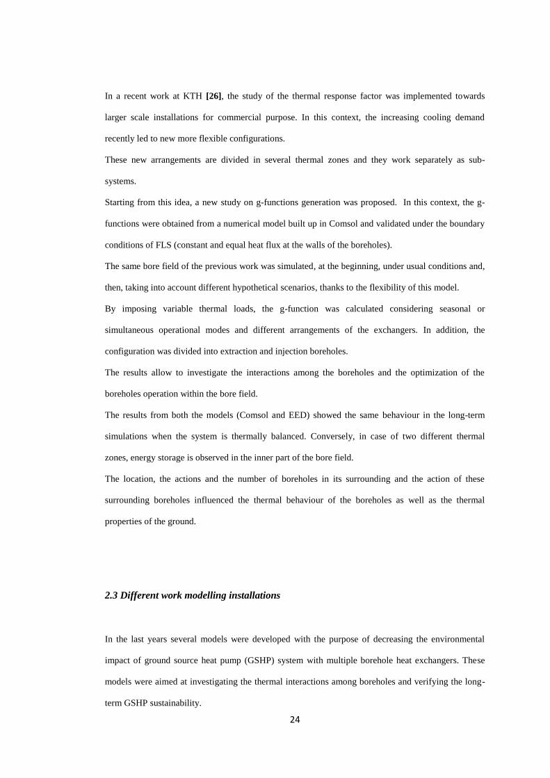
In the Figure 3.1 we can see the installation’s site.

Figure 3.1: View of the installation site

My project relies on the simulation of a large ground source heat pump installation of 130 boreholes

drilled surrounding the building. It is important to mention that the project concerns an uneven bore

field configuration, owing to constrains related to the available space around the planned building and

31

to the positions of the existing buildings. In addition, so many other factors often don’t allow to have a

regular borehole configuration.

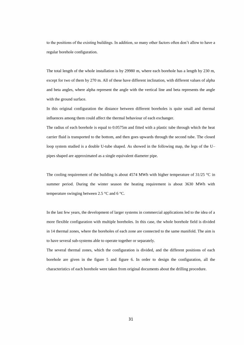
The total length of the whole installation is by 29980 m, where each borehole has a length by 230 m,

except for two of them by 270 m. All of these have different inclination, with different values of alpha

and beta angles, where alpha represent the angle with the vertical line and beta represents the angle

with the ground surface.

In this original configuration the distance between different boreholes is quite small and thermal

influences among them could affect the thermal behaviour of each exchanger.

The radius of each borehole is equal to 0.0575m and fitted with a plastic tube through which the heat

carrier fluid is transported to the bottom, and then goes upwards through the second tube. The closed

loop system studied is a double U-tube shaped. As showed in the following map, the legs of the U–

pipes shaped are approximated as a single equivalent diameter pipe.

The cooling requirement of the building is about 4574 MWh with higher temperature of 31/25 °C in

summer period. During the winter season the heating requirement is about 3630 MWh with

temperature swinging between 2.5 °C and 6 °C.

In the last few years, the development of larger systems in commercial applications led to the idea of a

more flexible configuration with multiple boreholes. In this case, the whole borehole field is divided

in 14 thermal zones, where the boreholes of each zone are connected to the same manifold. The aim is

to have several sub-systems able to operate together or separately.

The several thermal zones, which the configuration is divided, and the different positions of each

borehole are given in the figure 5 and figure 6. In order to design the configuration, all the

characteristics of each borehole were taken from original documents about the drilling procedure.

32

Figure 3.2: Configuration of several zones

Figure 3.3: Sketch of the borehole field geometry to be studied

Each coordinate (x,y) has been found by locating the centre of the borehole in the middle point

between the U-pipes. The inclined boreholes required to know the alpha and beta inclination.

0

20

40

60

80

100

120

140

-20 30 80 130

Y [

m]

X [m]

Boreholes field geometry

33

Alpha represents the angle from the perpendicular line to the ground surface (z axis) and beta is the

inclination of the borehole in the x,y plane.

In the different drilling descriptions available, the groundwater level was measured for each borehole

in all manifolds. The measured values of this level range from 4.2 m to 9.05 m. This level describes

where the heat exchange starts, and is used to define active part of the borehole in the heat exchange.

It is important to highlight the different values of the ratio D/H for the boreholes of this configuration.

In his previous work, Eskilson didn’t take into account the influence of D on the heat exchange. Only

in the recent studies, as shown by Cimmino and Bernier (2013) and Monzò (2014), the inactive part of

the borehole could influence the simulation and the results, especially in case of short boreholes.

In addition, each borehole is characterized by a measurement system with a yellow pipe and cables all

along these pipes, as showed in the following photo.

Figure 3.4: Measurement system

In every zone we can find the “measurement well” or “measurement manifold”, which measures the

flow rate and the temperature difference to each specific borehole.

34

4. METHODOLOGY

4.1 Approach carried out in the study

The work, started In March 2015 at the Department of Energy Technology of KTH, was led until

September 2015. It represents a preliminary study about the new settled system in Frescati area, which

is going to fulfil the new building’s energy requirement starting from the next month.

One of the aims of this work is to study the performance and the effects of the use of GSHPs in a

commercial building for both short and long time step operation.

In GHSP systems, which uses the ground as key source or sink to supply the heating and cooling

demand, it is really important to study the ground behaviour where such system is placed. The change

of ground temperature and, as a consequence, the fluid temperature will modify the heat pump

system’s performance.

In order to simulate the thermal process in an uneven bore field configuration and predict the fluid

temperature for the predicted case, it is important to explain clearly the methodology carried out.

At the beginning, a preliminary literature review about the topic of the assigned work was required to

be familiar with the body of science and follow the main theories up.

The Lamarche and Beauchamp’s theories gave an important contribution in this field and stand for the

base on which my work relies. Earlier the main theory was proposed by Eskilson in 1987, who was

the first to introduce a method based on non-dimensional thermal responses called “g-functions”. He

takes into account only even borehole configurations and for this reason his theory is characterized by

a lack of flexibility.

Then, in 2006, Lamarche and Beauchamp showed a different approach modelled on computing the

“g-functions” in an analytical way, for the medium and long time analyses of bore field configuration.

They provided many scripts for g-function calculations.

35

Gradually new models, either numerical or analytical, were also proposed in order to generate the “g-

functions” and analyse the thermal response of vertical heat exchangers.

Later than their first approach, Lamarche and Beauchamp developed a new analytical solution giving

an important contribution to the modelling of geothermal heat exchangers for short time transient

response. All these works were proposed for vertical boreholes. Following, they introduced a new

method for the calculation of time response factors for inclined boreholes.

A new technological development is placed in the last studies of Bernier and Cimmino. In addition, an

important contribution was given by KTH in the last few years.

Once I got familiar with the theory, the second task was to get along with the Matlab code. I started

observing and studying the code in order to understand how it works and to simulate the concerned

field.

The code was designed by Marc Derouet, in his previous master thesis, and then I had to update and

adapt it for my new configuration.

In the meanwhile, I started designing part of the real installation, previously described, in order to

arrange the input data about the bore field. I drew the configuration in order to know the right

coordinates and inclinations of each borehole.

At this stage, a large scale installation of 130 boreholes can be modelled and simulated following a

specific criteria.

The aim of this simulation was to assess the borehole wall and fluid temperature changes by

increasing the number of borehole studied in each of the simulations done. For this reason, firstly only

one borehole was simulated, and then a couple of boreholes close to each other. Gradually the whole

installation was simulated by evaluating separately the single manifolds and taking into account the

couples of closest manifolds.

The main purpose is to compare the behaviour of one borehole to a group of them in order to know

how neighbours could influence each other.

36

Each of these cases was simulated by dividing proportionally the total heat load, depending on the

total active length in each of them. It means to subtract the ground water level from the total length of

the simulated boreholes.

Once the methodology was clarified, the following task, before starting the simulations, was to check

the validity of the code with the last approach (FLS – Uniform Temperature, Bernier and Cimmino)

found in the literature. This preliminary check was necessary to find possible mistakes.

The code is validated by imposing a constant heat flux at the borehole wall in all the boreholes, as

boundary conditions. The model, given for this project, was built up according to the boundary

conditions described in the FLS method. For this reason, the values obtained from the code are

compared with the FLS solution of Bernier and Cimmino for a reference geometry with 2x3 BHEs in

a rectangular pattern (rb/H = 0.0004, D/H = 0.0343).

Figure 4.1 shows the g-function obtained from the code, named in the figure as “FLS – constant q”,

and that from the pre-processor, named “FLS – constant q reference”.

It is important to mention that the code gave different results in comparison with the values obtained

by pre-processor. Both of the approaches, for the generation of the g-function, use the same boundary

condition: that is uniform heat extraction rate along the length of the boreholes.

The difference, between the g-function calculated by the pre-processor and the g-function obtained by

the implemented code, increases with the value of ln(t/ts).

37

Figure 4.1: Comparison between the g-function values obtained with the Matlab code and the FLS reference case for a

configuration with different values of D/H for all the boreholes

It is clear as the difference, between the two curves, starts still before one year step operation, which is

placed up to a time ln(t/ts) = -4,6.

These curves were calculated in case of a vertical boreholes configuration with different values of

D/H.

Hereafter, using the same values of D/H for every boreholes, the gap between the two curves start to

be noticeable after one year operation, as shown on Figure 4.2.

In case of similar boundary condition at the borehole walls, the comparison with the FLS reference

case shows a perfect match between the two curves. Instead a small difference is observed for a

different reference case, with uniform borehole wall temperature along the length of the boreholes.

The g-functions are linear up to a time ln(t/ts) = -5 and then the slope of the curves increases. They

start to stabilize toward their steady-state value around time ln(t/ts) = 0, when axial effect become

significant.

0

2

4

6

8

10

12

14

16

18

-14 -12 -10 -8 -6 -4 -2 0 2 4 6 8 10

g-f

un

ctio

n v

alu

es

ln (t/ts)

G-function comparison

FLS - constant q reference

FLS - constant q

38

Figure 4.2: Comparison between the g-function values obtained with the Matlab code and the FLS reference case for a

configuration with the same values of D/H for all the boreholes

From these results, in order to continue working with this code, a new arrangement geometry was

designed, following the pre-processor for fields of vertical boreholes. Once defined the new geometry,

it was possible to determinate the g-function for both of the studied cases.

The g-functions are not the final goal of this work. The following step was to define the heat load

profile in order to assess the borehole wall and fluid temperatures for each case.

These temperatures were calculated for short and long term operation. The simulation time for short

term operation is 1 year, using an hourly load profile. For long term simulation of 20 years, a heat

load profile with monthly step was used. The heat load profile of the first year was extended for the

following 20 years.

0

2

4

6

8

10

12

14

16

18

-14 -12 -10 -8 -6 -4 -2 0 2 4 6 8 10

g-f

un

ctio

n v

alu

es

ln (t/ts)

G-function comparison

FLS - uniform T reference

FLS - constant q reference

FLS - constant q

39

4.2 New BHEs arrangement

As the comparison shown previously, the Derouet’s code was not able to calculate accurately the g-

functions’ values, owing to different values of the ratio D/H for all the boreholes.

For this reason, it was necessary to come up with an alternative resolution. The whole installation was

studied taking into consideration separately each manifold, after ensuring that no thermal interaction

occurs among them.

The new arrangement geometry was designed placing each borehole’s coordinates (x,y) in the middle

point of the real boreholes. This configuration is shown in the Figure 4.3.

Figure 4.3: BHE configuration for straight boreholes taking into account the middle point for each borehole of original

geometry

The first consequence of this approximation was the increase of spacing among the boreholes. For this

reason, the distance between two different manifolds has to be verified thereby ensuring the spatial

temperature distributions would not cross to avoid any interactions.

0

20

40

60

80

100

120

140

160

-20 30 80 130

Y [

m]

X [m]

Approximated borehole field geometry

Manifold 1

Manifold 2

Manifold 3

Manifold 4

Manifold 5

Manifold 6

Manifold 7

Manifold 8

Manifold 9

Manifold 10

Manifold 11

Manifold 12

Manifold 13

Manifold 14

40

If the boreholes from different manifolds don’t see each other in the timeframe of 6 months to 1 year,

it will be possible to study separately the manifolds to assess the whole installation.

According to the theory of Göran Hellström (1991), the penetration depth for each couple of

manifolds was calculated and compared to the spacing among adjacent heat exchangers in order to

assess the thermal influence between manifolds. It is a characteristic length for the periodic

temperature variation in the ground and can be expressed as:

𝑑𝑝 = √𝛼𝑡𝑝

𝜋 (5)

It depends on the thermal diffusivity α and the period time tp and only 5% of the amplitude remains at

a depth 3dp from the boundary [33].

Each manifold is judged using a hexagonal duct pattern, so in this case the influence is negligible

when:

𝑟′1 = 𝑟1√2 𝜋

𝑎 𝑡𝑝≥ 3 (6)

Where “r1” is the outer boundary for each manifold, “a” is the ground thermal conductivity and “tp” is

the period time.

Taking the ground thermal conductivity equal to 1.62*10-6 m2/s and r1 equal to the distance between

two boreholes from different manifolds, we found that just for two couples of manifolds the spacing is

comparable to the penetration depth. It means that a moderate thermal influence is observed after 1

year step operation between these two couples. For all other cases it is possible to study separately

each manifold in order to analyse all installation.

Since the value of r’1 is less than 3 for the couples of manifolds 3-4 and 5-6, both of them will be

simulated separately and then also together in order to show how change the thermal behaviour.

41

4.3 Assumptions made

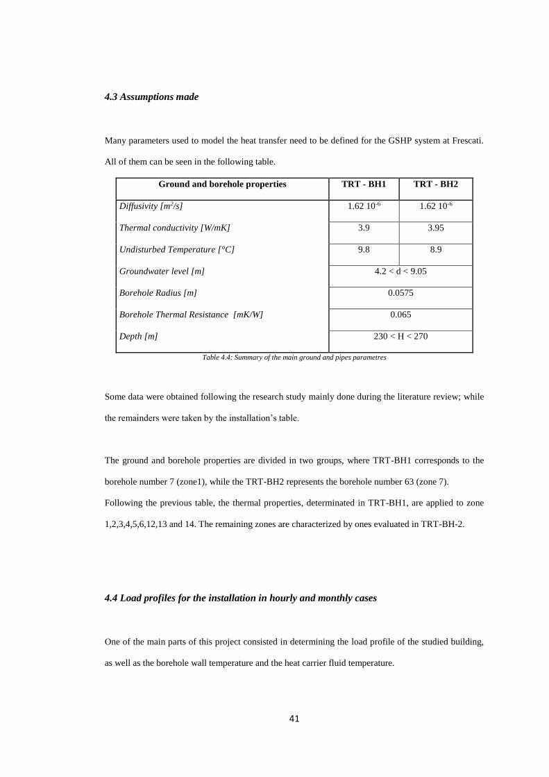
Many parameters used to model the heat transfer need to be defined for the GSHP system at Frescati.

All of them can be seen in the following table.

Ground and borehole properties TRT - BH1 TRT - BH2

Diffusivity [m2/s] 1.62 10-6 1.62 10-6

Thermal conductivity [W/mK] 3.9 3.95

Undisturbed Temperature [°C] 9.8 8.9

Groundwater level [m] 4.2 < d < 9.05

Borehole Radius [m] 0.0575

Borehole Thermal Resistance [mK/W] 0.065

Depth [m] 230 < H < 270

Table 4.4: Summary of the main ground and pipes parametres

Some data were obtained following the research study mainly done during the literature review; while

the remainders were taken by the installation’s table.

The ground and borehole properties are divided in two groups, where TRT-BH1 corresponds to the

borehole number 7 (zone1), while the TRT-BH2 represents the borehole number 63 (zone 7).

Following the previous table, the thermal properties, determinated in TRT-BH1, are applied to zone

1,2,3,4,5,6,12,13 and 14. The remaining zones are characterized by ones evaluated in TRT-BH-2.

4.4 Load profiles for the installation in hourly and monthly cases

One of the main parts of this project consisted in determining the load profile of the studied building,

as well as the borehole wall temperature and the heat carrier fluid temperature.

42

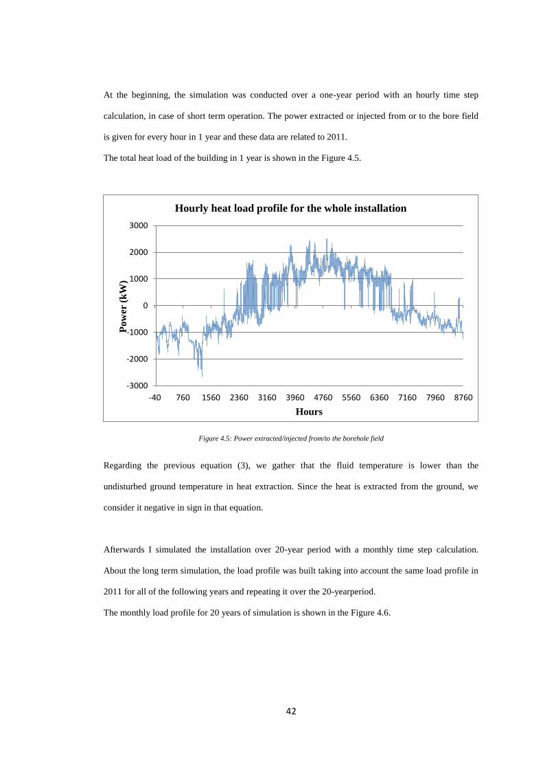
At the beginning, the simulation was conducted over a one-year period with an hourly time step

calculation, in case of short term operation. The power extracted or injected from or to the bore field

is given for every hour in 1 year and these data are related to 2011.

The total heat load of the building in 1 year is shown in the Figure 4.5.

Figure 4.5: Power extracted/injected from/to the borehole field

Regarding the previous equation (3), we gather that the fluid temperature is lower than the

undisturbed ground temperature in heat extraction. Since the heat is extracted from the ground, we

consider it negative in sign in that equation.

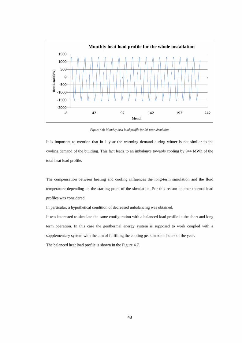
Afterwards I simulated the installation over 20-year period with a monthly time step calculation.

About the long term simulation, the load profile was built taking into account the same load profile in

2011 for all of the following years and repeating it over the 20-yearperiod.

The monthly load profile for 20 years of simulation is shown in the Figure 4.6.

-3000

-2000

-1000

0

1000

2000

3000

-40 760 1560 2360 3160 3960 4760 5560 6360 7160 7960 8760

Pow

er (

kW

)

Hours

Hourly heat load profile for the whole installation

43

Figure 4.6: Monthly heat load profile for 20-year simulation

It is important to mention that in 1 year the warming demand during winter is not similar to the

cooling demand of the building. This fact leads to an imbalance towards cooling by 944 MWh of the

total heat load profile.

The compensation between heating and cooling influences the long-term simulation and the fluid

temperature depending on the starting point of the simulation. For this reason another thermal load

profiles was considered.

In particular, a hypothetical condition of decreased unbalancing was obtained.

It was interested to simulate the same configuration with a balanced load profile in the short and long

term operation. In this case the geothermal energy system is supposed to work coupled with a

supplementary system with the aim of fulfilling the cooling peak in some hours of the year.

The balanced heat load profile is shown in the Figure 4.7.

-2000

-1500

-1000

-500

0

500

1000

1500

-8 42 92 142 192 242

Hea

t L

oa

d (

kW

)

Month

Monthly heat load profile for the whole installation

44

Figure 4.7: Balanced heat load profile

For short and long term simulations, both the unbalanced and balanced heat load profile was used with

special attention to the starting operation month.

The first simulation were started in January, and then the start-up point were made overlap with the

real start-up of the geothermal system (October 2015). Starting the simulation in another month means

to shift the load profile with possible consequences on the heat carrier fluid temperature.

The aim is to minimize the fluid temperature and therefore maximize the heat pump performance.

-3000

-2500

-2000

-1500

-1000

-500

0

500

1000

1500

-240 760 1760 2760 3760 4760 5760 6760 7760 8760

Po

wer (

kW

)

Hours

Balanced Heat Load Profile starting from January

45

46

5. RESULTS

With the purpose of figuring out clearly the results, a brief introduction to the executive procedure is

presented.

For each case study, the short and long term simulations were carried out considering different

hypothesis and all of the results obtained from the simulations done can be summarized in three

following steps:

First step: the new geometry arrangement was simulated with hourly and monthly load

profiles for the predicted case (Unbalanced load profile).

Second step: A special attention to the starting operation month was given in order to

evaluate the performance improvement.

Third step: A Balanced heat load profile was supposed in order to decrease the long-term

effect of the thermal drift.

5.1 G-function for the borehole field in Frescati

Once validated the code with last approaches, after a long comparison, and designed the new

geometry arrangement, the g-functions for each study case were calculated using the updated Matlab

code.

The code was previously updated and validated related to the uneven bore field with vertical

boreholes, where their coordinates have been illustrated earlier, and with same values of ratio D/H.

The g-function values for each study cases are presented as a function of the non-dimensional time

ln(t/ts) in Figure 5.1.

47

Figure 5.1: G-function of the Frescati installation for each study case

For single borehole and couple of boreholes, the curves are linear in the first region of the graph, up to

a time ln(t/ts) = -6. In this region, the temperature is uniform along the height and it varies only in

radial direction. It is noticeable that all the curves are completely matched. This means that the

borehole spacing is not relevant.

In this part of the graph, the axial conduction effects are negligible for small values of time and the

heat transfer is only in the radial direction. In addition the spacing B among boreholes was rather

increased after the approximation to vertical boreholes.

These factors ensure that thermal interaction among boreholes is almost negligible and the g-function

for couple of boreholes is similar to the g-function for a single borehole.

For the other cases, the slope of the g-function curves increases before ln(t/ts) = -5 and after that the

thermal interactions among boreholes become important. The boreholes will start to interfere with

each other after some months of operation. In this second range time, until when the curves don’t

reach the steady-state, the heat transfer is studied in radial and axial direction. The g-function value

increase depends on the number of the boreholes in the relative case and on the geometrical layout, as

it can be seen between Manifold 1 and Manifold 3.

02468

10121416182022242628303234363840

-13 -12 -11 -10 -9 -8 -7 -6 -5 -4 -3 -2 -1 0 1 2 3 4 5 6 7 8 9

g-fu

nct

ion

val

ues

ln (t/ts)

Frescati's g-functions

Single borehole

Couple of Boreholes

Manifold 1

Manifold 3

Couple of Manifolds

48

The last part of the graph represents the steady-state heat transfer and it starts from ln(t/ts) = -2, which

corresponds to 16 years. For very long time the bore field and the ground are in equilibrium and the

extraction does not affect the borehole wall temperature.

5.2 About the short term simulation with hourly heat load profile

At this stage, after validated the code concerning the new approximated configuration, it was possible

to use the pre-calculated g-function in order to simulate the thermal behaviour of the bore field and to

obtain the hourly and monthly variation of the borehole wall and fluid temperatures.

The fluid temperatures were calculated with variable heat load profiles by temporal superposition to

account for the time variation of the heat extraction rates of individual boreholes.

Since there are no interactions between manifolds, according to the calculation of the penetration

time, the load is distributed proportionally to the total length of each manifold. Thus, the total load

profiles will be divided equivalently depending on the ratio between the total length of the examined

boreholes and the total length of the whole borehole field.

At the beginning, the system has been studied in 1-year time operation, dividing the simulation in

different cases:

Simulation of one borehole (the borehole number 1 in the zone 1 is taken as reference);

Interactions between a couple of boreholes in the same manifold;

Simulation of one manifold;

Simulation of a couple of close manifolds (manifold 3 and 4).

The variation of the heat carrier fluid temperature, due to a variable heat extraction rate for 1 year of

hourly simulation, is shown for all study cases.

49

All of these cases are summarized in the Figure 5.2:

Figure 5.2: Heat carrier fluid temperature profile from the simulation starting in January with an unbalanced load profile

Single

Borehole

Couple of

Boreholes Manifold 1 Manifold 3

Couple of

Manifolds

Tf max [°C] 29.94 29.98 30.13 29.93 29.55

Tf min [°C] -11.85 -12.07 -13.1 -13.39 -13.72

Table 5.1: Maximum and minimum values of the heat carrier fluid temperature for a simulation starting in January with an

unbalanced load profile

The attention is focused on the temperature of the heat carrier fluid, which represents a key parameter.

A synthesis of the annual minimum and maximum temperature of the fluid is outlined in Figure 2 and

summarized numerically in the Table 5.1.

Since the annual amount of heat extracted from the ground is lower than that which is injected into the

ground, the long term fluid temperature inside the ground heat exchangers increase, as it is noticed by

the simulation.

-16-14-12-10

-8-6-4-202468

10121416182022242628303234

01/01/2011 00:00 11/04/2011 00:00 20/07/2011 00:00 28/10/2011 00:00

Tem

per

atu

re (

°C)

Hours

Tf comparison between different study cases

Tf - Single Borehole

Tf - Couple of Boreholes

Tf - Manifold 3

Tf - Couple of Manifolds

50

By and large, a similar shape of the curves can be observed for all cases. The maximum temperature

of the fluid is quite similar for all of the cases, amounting to 30 °C.

Obviously, the maximum efficiency is achieved when the maximum temperature change is kept to a

minimum. In addition an extreme local heating of the ground is not desirable, since it could modify

the efficiency of the heat pump.

For these reasons the idea was to use different heat load profiles in order to assess the fluid

temperature change in comparison with the predicted case and determine the possible improvement by

a more balanced use of the ground.

Two ways were proposed in this project:

The first way was to start the simulation in October, maintaining the same hourly energy

profile.

The second way was to use a balanced heat load profile, by coupling the geothermal system

with a supplementary system which would be started up during the hours of cooling peaks.

5.2.1 Starting point in October

With the same unbalanced heat load profile, the same study cases were simulated moving up the

starting operation month in October.

The results of the new simulation were compared with that originally simulated. The difference

temperature (in Kelvin) was plotted in the Figure 5.3.

51

Figure 5.3: Comparison between two simulations starting in October and in January with an unbalanced load profile

The hourly values of fluid temperature in 1-year time operation decreased by about 5,2 K at the

beginning of January (after 2000 hours). The temperature difference decreases quickly and in April

(after 5000 hours) it is less than 1 K for all of the cases.

Concerning only the annual maximum value, no improvements are obtained with this strategy.

5.2.2 Balanced load profile

When the energy flow imbalance was reduced and the unbalanced load profile was replaced with a

balanced load profile, the maximum fluid temperature was decreased by around 9 K from the original

value.

Comparing the results obtained by simulating a balanced load profile starting in January with the

original result in same starting operation month, the hourly temperature difference between these two

cases is shown in the Figure 5.4.

0

1

2

3

4

5

6

0 2000 4000 6000 8000 10000 12000

Tem

per

atu

re d

iffe

ren

ce (

K)

Hours

Temperature difference October - January

Single Borehole

Couple of Boreholes

Maifold 1

Manifold 3

52

Figure 5.4: Comparison between unbalanced and balanced load profile in the same starting operation month

In the time frame when the cooling peak was supplied by the alternative system, the hourly

temperature difference can reach the value of 7 K, leading to a great improvement of the heat pump

efficiency.

When the extracted energy flow is equal to the injected energy flow, a good improvement of the

maximum fluid temperature is reached and shown in the Table 5.2.

Single

Borehole

Couple of

Boreholes Manifold 1 Manifold 3

Couple of

Manifolds

Unbalanced

Load Profile

Tf max [°C] 29.94 29.98 30.13 29.93 29.55

Tf min [°C] -11.85 -12.07 -13.1 -13.39 -13.72

Balanced

Load profile

Tf max [°C] 20.22 20.5 21.57 21.91 22.85

Tf min [°C] -11.85 -12.07 -13.11 -13.4 -14.58

Table 5.2: Maximum and minimum values of the fluid temperature in case of unbalanced and balanced heat load profile

0

1

2

3

4

5

6

7

8

-1330 670 2670 4670 6670 8670

Tem

per

atu

re d

iffe

ren

ce (

K)

Hours

Temperature difference Unbalanced-Balanced

Single Borehole

Couple of Boreholes

Manifold 1

Manifold 3

Couple of Manifolds

53

Then, the same balanced heat load profile was used to simulate the temperature changes starting in

October. But the difference between the two cases is the same, as we recorded in case of unbalanced

load profile.

5.3 About the long term simulation with monthly heat load profile

In the previous paragraph, the short-term simulation, with an hourly time resolution, allowed to assess

the minimum and maximum temperature of the heat carrier fluid, which represents a relevant design

parameter.

Now the attention shifts to the long-term simulation in order to evaluate the effect of a periodic heat

load in each study case under the same considerations previously introduced.

In this section, a monthly time resolution is required in order to outline the evolution of the fluid

temperature in 20-year time operation. The results have been calculated considering the predicted heat

load profile of the first year, used in the short-time simulations, for all the following 20 years of

operation.

The borehole wall temperature and the heat carrier fluid temperature are plotted together and they are

presented in Figure 5.5, Figure 5.6, Figure 5.7 and Figure 5.8, for the cases of single borehole, couple

of boreholes, manifold 3 and couple of manifolds.

54

Figure 5.5: Borehole wall temperature and heat carrier

fluid temperature profiles for a single borehole with

monthly loads

Figure 5.6: Borehole wall temperature and heat carrier

fluid temperature profiles for a couple of boreholes with

monthly loads

Figure 5.7: Borehole wall temperature and heat carrier

fluid temperature profiles for the manifold 3 with monthly

loads

Figure 5.8: Borehole wall temperature and heat carrier

fluid temperature profiles for a couple of manifolds with

monthly loads

Several observations arise from these results. At first, the tendency of the periodic curves is quite

similar for both the single borehole and couple of boreholes cases. This is due to the huge ground

volume surrounding each borehole after having taken the approximated geometry.

Since the borehole separation distance is about 15 m, in case of studying a couple of boreholes,

thermal interferences doesn’t affect the behaviour of individual boreholes in a long-term heat process.

-5

0

5

10

15

20

25

30

0 50 100 150 200

Tem

pe

ratu

re (°

C)

Month

Single BoreholeTb

Tf

-5

0

5

10

15

20

25

30

0 50 100 150 200

Tem

pe

ratu

re (°

C)

Month

Couple of Boreholes Tb Tf

-10

-5

0

5

10

15

20

25

30

0 100 200

Tem

ep

ratu

re (°

C)

Month

Manifold 3Tb

Tf

-10

-5

0

5

10

15

20

25

30

35

0 100 200

Tem

pe

ratu

re (°

C)

Months

Couple of Manifolds Tb

Tf

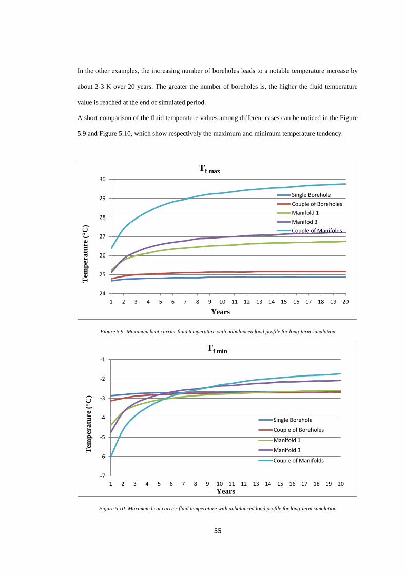
55

In the other examples, the increasing number of boreholes leads to a notable temperature increase by

about 2-3 K over 20 years. The greater the number of boreholes is, the higher the fluid temperature

value is reached at the end of simulated period.

A short comparison of the fluid temperature values among different cases can be noticed in the Figure

5.9 and Figure 5.10, which show respectively the maximum and minimum temperature tendency.

Figure 5.9: Maximum heat carrier fluid temperature with unbalanced load profile for long-term simulation

Figure 5.10: Maximum heat carrier fluid temperature with unbalanced load profile for long-term simulation

24

25

26

27

28

29

30

1 2 3 4 5 6 7 8 9 10 11 12 13 14 15 16 17 18 19 20

Tem

per

atu

re (°C

)

Years

Tf max

Single Borehole

Couple of Boreholes

Manifold 1

Manifod 3

Couple of Manifolds

-7

-6

-5

-4

-3

-2

-1

1 2 3 4 5 6 7 8 9 10 11 12 13 14 15 16 17 18 19 20

Tem

per

atu

re (°C

)

Years

Tf min

Single Borehole

Couple of Boreholes

Manifold 1

Manifold 3

Couple of Manifolds

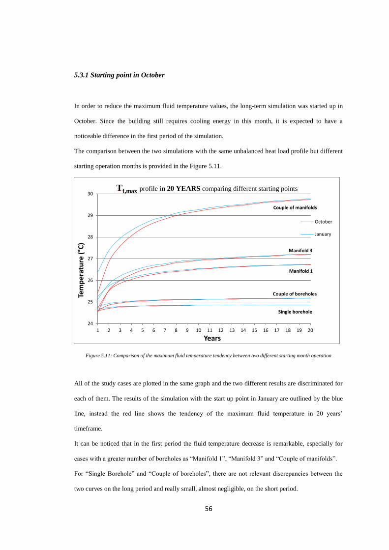
56

5.3.1 Starting point in October

In order to reduce the maximum fluid temperature values, the long-term simulation was started up in

October. Since the building still requires cooling energy in this month, it is expected to have a

noticeable difference in the first period of the simulation.

The comparison between the two simulations with the same unbalanced heat load profile but different

starting operation months is provided in the Figure 5.11.

Figure 5.11: Comparison of the maximum fluid temperature tendency between two different starting month operation

All of the study cases are plotted in the same graph and the two different results are discriminated for

each of them. The results of the simulation with the start up point in January are outlined by the blue

line, instead the red line shows the tendency of the maximum fluid temperature in 20 years’

timeframe.

It can be noticed that in the first period the fluid temperature decrease is remarkable, especially for

cases with a greater number of boreholes as “Manifold 1”, “Manifold 3” and “Couple of manifolds”.

For “Single Borehole” and “Couple of boreholes”, there are not relevant discrepancies between the

two curves on the long period and really small, almost negligible, on the short period.

24

25

26

27

28

29

30

1 2 3 4 5 6 7 8 9 10 11 12 13 14 15 16 17 18 19 20

Tem

per

atu

re (

°C)

Years

Tf,max profile in 20 YEARS comparing different starting points

October

January

Single borehole

Couple of boreholes

Manifold 1

Manifold 3

Couple of manifolds

57

These observations certify that the starting operation month doesn’t affect the results neither in the

short period nor in the long period and when considering an increasing number of boreholes there are

more interactions.

5.3.2 Balanced load profile

As last result, it is worthwhile to compare the maximum fluid temperature tendency in 20–year

operation in case of unbalanced and balanced load profile.

For both load profiles, the simulations started in October and all of the study cases are shown in

Figure 5.12.

Figure 5.12: Comparison of the maximum fluid temperature tendency between unbalanced and balanced heat load profile

19

20

21

22

23

24

25

26

27

28

29

30

1 2 3 4 5 6 7 8 9 10 11 12 13 14 15 16 17 18 19 20

Tem

epra

ture

(°C

)

Years

Tf,max profile in 20 years comparing Balanced and Unbalanced profile

Balanced - Single Borehole

Unbalanced - Single Borehole

Balanced - Coupel of Boreholes

Unbalanced - Couple of Boreholes

Balanced - Manifold 1

Unbalanced - Manifold 1

Balanced - Manifold 3

Unbalanced - Manifold 3

Balanced - Couple of Manifolds

Unbalanced - Couple of Manifolds

UNBALANCED

BALANCED

58

In the plot, the red lines outline the fluid temperature tendency over 20 years using the original and

unbalanced load profile. The fluid temperature, reached at the end of each simulation, change

considerably going from “single borehole” case to “manifold” case, and from “manifold” case to

“group of manifolds” case as well.

On the other hand, the blue lines show that a balanced load profile reduce the distance between them

and the fluid temperature difference between the “single borehole” case and “couple of manifolds”

case is lower than 2 K during the long-term simulation.

It is interesting to notice that using a balanced load profile allows to have a good efficiency

improvement since the heat carrier fluid temperatures are much lower than that obtained with an

unbalanced load profile.

Moreover the different load profile influences the slope of the curves in the first period of the

simulation. As regards to the unbalanced cases, it can be also noticed that the temperature increases up

to about 2 K in the first 4 years. Instead it is less than 1 K when the heat load profile is balanced.

Concerning the minimum fluid temperature, the tendency for both unbalanced and balanced load

profile is shown in the Figure 5.13.

59

Figure 5.13: Comparison of the minimum fluid temperature tendency between unbalanced and balanced heat load profile

As we expected, the balanced load profile reduce the slope of all curves in the first years of operation

and then all of the curves tends to become linear after few years.

Reducing the heat injected in the ground in summer time increased the impact of the heat extraction

process in winter time, with a decrease of the minimum fluid temperature. This decrease is remarkable

when the number of boreholes simulated is high. The minimum temperature can decrease up to 4 K in

the case of “group of manifolds”.

-8

-7

-6

-5

-4

-3

-2

-1

1 2 3 4 5 6 7 8 9 10 11 12 13 14 15 16 17 18 19 20

Tem

per

atu

re (

°C)

Years

Tf min profile in 20 years comparing Balanced and Unbalanced profile

Balanced - SingleBorehole

Balanced - Couple ofBoreholes

Balanced - Manifold 1

Balanced - Manifold 3

Balanced - Couple ofManifolds

Unabalanced - SingleBorehole

Unbalanced - Couple ofboreholes

Unbalanced - Manifold 1

Unabalanced - Manifold 3

Unabalnced - Couple ofManifolds

60

6. DISCUSSION AND LIMITATIONS

This experimental study where alternative operational modes have been introduced provided many

useful results in order to have a notable evaluation of a real GSHP installation in Stockholm. These

results allow us to investigate on the thermal interactions among boreholes and on the optimization of

the GSHP system’s performance. They represent the baseline for beginning to discuss possible

solutions.

The aim of the study was to judge the accuracy of the simulation code in the perspective of describing

properly the thermal response of the borehole heat exchangers configuration. For this reason it is

important to explain the assumptions done and their influences on the final results.

The code has been taken from a previous work. In that case, it was developed to evaluate the thermal

response of a GSHP installation of 26 boreholes arranged in a symmetrical pattern and divided in two

different thermal zones.

The given simulation code, run with the software Matlab, showed initially a small inaccuracy in the

computation of the g-functions related to committed bore field.

The code was built up according to the boundary conditions described in the FLS approach of

Lamarche and Beauchamp (constant heat flux at the borehole’s wall). For its validation, the model

was compared with the new FLS analytical solution proposed by Bernier and Cimmino, taking into

consideration two different boundary conditions (constant heat flux at the borehole’s wall and uniform

borehole wall temperature equal for all boreholes).

The g-function calculated by the code was compared with those calculated by the new FLS method.

This comparison was carried out for two kinds of standard configurations (2x3 BHEs with vertical

boreholes in a rectangular pattern), one having same values of D/H and the other having different

values of D/H.

Only in the first case the comparison gave satisfying results throughout the timeframe.

61

Since the geometry presents different values of groundwater levels and borehole depths, it must be

said that the given model overestimates the configuration committed in this project.

Thus, a new solution was found with the purpose of solving this problem and continuing to work with

the given code.

The real geometry was approximated according to the theory of Hellström and the new arrangement

was designed. This is a crucial point since the hypothesis on the geometry will influence the results at

end of the work.

In the approximated geometry the distance between boreholes is rather larger than that in the real case

and, as a consequence, this mitigates the thermal interferences between them.

For this reason, it is necessary an additional validation of the model with the on-site measurements

data. A limitation, highlighted also in the previous work, is that such projects need the data acquisition

on the installation.

It has been important to have pointed out these assumptions related to the new geometry’s

arrangement and the limitations found on the code, since they could influence the final results.

Another aspect to mention is that the thermal behaviour of the bore field was simulated considering

hourly steps in the short-term modelling. In spite of the increasing computational time, the choice to

work with hourly steps gives more accurate results instead of using daily or monthly ones as in the

previous modelling.

Once the critical points are overcome, it was possible to start the simulations in order to predict how

the ground will behave.

62

7. CONCLUSIONS

The project, which was entrusted to me during my exchange period in Stockholm, mainly concerns

the study of a large scale GSHP system. The installation is composed of 130 boreholes with different

inclinations and groundwater levels.

The boreholes are arranged in an uneven geometry divided in 14 thermal zones, each one are

connected to a different heat pump. It is important to mention that the thermal influences among most

of them were estimated negligible.

The simulation of the thermal process for the given bore field configuration aims at predicting the heat

carrier fluid temperature for short-term (1 year) and long-term (20 years) simulations, considering

respectively hourly and monthly load profiles. The knowledge of the borehole exit fluid temperature is

important to assess and optimize the performance of the GSHP installation.

The thermal response of the borehole is studied by a short-term simulation. Conversely, the study of

thermal interactions among boreholes is a slow process and takes more time, and it depends upon the

extraction and injection periods of the ground heat.

After becoming familiar with the simulation software, the second step was to design the field layout

and, at the same time, check the validity of the code. This preliminary check was required to find

possible mistakes in the model.

Since the code was not able to simulate properly the whole installation, it was necessary to come up

with an alternative resolution.

For this reason, the uneven configuration was approximated, taking into consideration only vertical

boreholes, and simulated considering separately the different thermal zones with the unbalanced heat

load profile.

In addition, different cases were studied considering an increasing number of boreholes in order to

assess the thermal influence among the exchangers on the fluid temperature drift.

63

Once the different study cases were defined and the field layout was acquired, the g-functions were

calculated for each case. The following step was to predict the heat carrier fluid temperature

circulating in the boreholes.

As regards the unbalanced load profile, the fluid temperature change due to an increasing number of

boreholes is notable, especially in the second part of the year.

In the long-term simulation, the thermal behaviour of a single borehole shows that the system seems

to be thermally balanced. The fluid temperature profile presents repetitive responses over the

simulation time. In fact, the peak-to-peak variation of the heat carrier fluid temperature is about 27 K

(maximum temperature around 24°C and minimum temperature around -3 °C) throughout 20 years.

In the first years, a greater number of boreholes increase the difference between the maximum and the

minimum value of the fluid temperature. After 5-6 years, the fluid temperature levels continue to

increase slightly until the end of the simulation time.

As a result, the minimum fluid temperature reached after one year for a couple of manifolds is about -

6 °C and the maximum one about 26 °C. At the end of the simulation period they are respectively

about -2 °C and 30 °C at the end of the simulation period.

On the basis of the results obtained, two hypothetical scenarios were introduced in order to point out

potential ways to improve the performance of the GSHP system. With this objective in mind, the

configuration was simulated using balanced load profiles and by changing the starting month

operation.

Firstly, starting the simulation in October, and not in January, does not lead to a notable improvement

of the system performance. This is partly due to the fact that the heat extracted, from October to

January, is around 20% of the heat injected during the rest part of the year.

In this case, the fluid temperature decreases by about 5 K at the beginning of January, while after

March the gap starts to be negligible.

64

The second alternative was to reduce the heat imbalance and simulate the approximated configuration

with a balanced load profile. In order to have the same cooling and heating demands supplied by the

geothermal system, a new supplementary cooling system was coupled with the GSHP system.

As expected, the hybrid GSHP system led to an improvement of the heat pump efficiency, especially

in summer time when the auxiliary technology is called to supply the cooling peak.

In 1 year of operation the maximum temperature decreased by 5 K and up to 8 K in the long-term

process.

With respect to the economic evaluation, it needs to assess the costs for potential auxiliary system (for

example solar panels or other solutions) to know the energetic and economic feasibility.

Further experimental analysis should be carried out in order to verify if the given model describes the

real behaviour of the system with sufficient accuracy.

The approximation done for the new geometry arrangement seems to be acceptable to simulate the

thermal process of the real configuration, even if the spacing between boreholes is larger with respect

to one of the real case.

Nevertheless a better validation of the model could be done by comparing the obtained results with

real values, which can be measured starting from October 2015.

Furthermore a new way of resolution was thought during the last meetings. The increasing interest of

cooling in the commercial buildings is leading towards more versatile configurations in order to fulfil

cooling and heating demand by dividing the ground into different thermal zones.

The usual way of operating multiple borehole fields today is to use all the BHEs to extract heat during

winter and inject it during summer.

As alternative operation mode, the manifolds of the same configuration could be split in two different

groups, extraction BHEs and injection BHEs. The idea is to use the boreholes of a group to supply the

heating energy and those of the other group to fulfil the cooling demand.

The purpose is to increase the spacing between groups of boreholes and reduce the thermal

interference in the long-term heat process.

65

66

REFERENCES

[1] John W. Lund, Tonya L. Boyd, 2015. Direct Utilization of Geothermal Energy 2015 Worldwide

Review. Proceedings World Geothermal Congress 2015, Melbourne, Australia.

[2] http://www.managenergy.net/lib/documents/922/original_Signhild_Gehlin__.pdf?1385983823

[3] International Energy Agency (IEA), Renewables for heating and cooling (2007).

[4] Lund J., Sanner B., Rybach L., Curtis R., Hellstrom G., Geothermal (Ground-Source) Heat Pumps:

a world overview.

[5] Signhild Gehlin, Olof Andersson, Leif Bjelm, Per-Gunnar Alm, Jan-Erik Rosberg. Country Update

for Sweden, Proceedings World Geothermal Congress 2015, Melbourne, Australia, 19-25 April 2015.

[6] Lind J., 2011. Swedish ground source heat pump case study (2010 version), GNS Science Report

2010/54, 30p.

[7] Håkan Sköldberg, Bo Rydén, The heating market in Sweden – an overall view (2014)

[8] SVEP Information and Service AV. www.svepinfo.se

[9] Gazo & Lind (2010). Gazo, F., Lind, L.: Low Enthalpy Geothermal Energy – Technology Review.

Institute of

Geological and Nuclear Sciences (GNS), Lower Hutt 2010

[10] Marc Derouet, 2014, Analysis of borehole heat exchanger in an existing ground-source heat

pump installation, KTH School of Industrial Engineering and Management.

67

[11] Philippe Dumas, Luca Angelino; Geothermal Market Report for Europe, Proceedings World

Geothermal Congress 2015, Melbourne, Australia.

[12] Kurevija T, Vulin D, Krapec V. Effect of borehole array geometry and thermal interferences on

geothermal heat pump system. Energy Conversion and Management 2012; 134 – 142.

[13] G. Hellstrom, Ground Heat Storage. Thermal Analysis of duct storage systems. Part 1 Theory,

Ph.D. thesis, University of Lund, Department of Mathematical Physics, Sweden, 1991

[14] Ingersoll L., Zobel O.: Heat conduction with engineering, geological, and other applications,

McGraw-Hill, (1954).

[15] Carlslaw H., Jaeger J.: Conduction of heat in solids, Oxford UK Claremore Press (1946).

[16] Eskilson P., Thermal analysis of heat extraction boreholes. Lund, Sweden. PhD thesis.

Department of mathematical physics, Lund Institute of Technology, 1987.

[17] Eskislon P., Temperature response function g for 38 borehole configurations, Dept. of

Mathematical Physics, Lund Institute of Technology, Lund, Sweden (1986).

[18] Eskislon P., Temperature response function g for 12 borehole configurations, Dept. of

Mathematical Physics, Lund Institute of Technology, Lund, Sweden (1987).

[19] H. Y. Zeng, N. R. Diao, Z. H. Fang, A finite line-source model for boreholes in geothermal heat

exchangers; Heat transfer Asian research 31 (7), 558 – 567.

[20] Lamarche L., Beauchamp B.; 2007, A new contribution to the finite line-source model for

geothermal boreholes. Energy and buildings, 39(2): 188 – 198.

68

[21] Lamarche L., Analytical g-function for inclined boreholes in ground-source heat pump systems.

Geothermics 40(2011); 241 - 249

[22] Claesson J., Javed S., An analytical method to calculate borehole fluid temperatures for time

scales from minutes to decades. (2011) ASHRAE Transactions, vol. 117(2), 279 – 288.

[23] Cimmino M, Bernier M., Adams F., 2013. A contribution towards the determination of g-

functions using the finite line source, Applied thermal engineering, 51(1-2), 401 – 412.

[24] Cimmino M., Bernier M., Preprocessor for the generation of g-functions used in the simulation of

geothermal systems.

[25] Acuna J., Fossa M., Monzò P., Palm B., Numerically generated g-functions for Ground Coupled

Heat Pump Applications, KTH, Royal Institute of Technology.

[26] Monzò, Acuna J., Mogensen P., Palm B., “A study of the thermal response of a borehole field in

winter and summer”, Internation Conference on Applied Energy (2013), KTH, Royal Institute of

Technology.

[27] Eskilson, Claesson, Simulation model for thermally interacting heat extraction boreholes (1998),

Numerical Heat Transfer 13, 149 – 165.

[28] Capozza A, Zarella A, De Carli M, Long-term analysis of two GSHP system using validated

numerical models and proposals to optimize the operating parameters. Energy and Buildings (2015);

50 – 64.

69

[29] Teza G, Galgaro A, De Carli M, Long-term performance of an irregular shaped borehole heat

exchanger system: Analysis of real pattern and regular grid approximation; Geothermics (2012); 45 –

56.

[30] Bayer P, de Paly M, Beck M, Strategic optimization of borehole heat exchanger field for seasonal

geothermal heating and cooling, Applied energy (2014), 445 – 453.

[31] Carslaw, Jaeger, 1959. Conduction of heat in solids. Oxford University Press, New York, NY,

USA, 510 pp.

[32] de Paly, Hecht-Mendez, Beck, Blum, Zell, Bayer, Optimization of energy extraction for closed

shallow geothermal systems using linear programming. Geothermics (2012); 57 – 65.

[33] Göran Hellström, Ground Heat Storage, Thermal analyses of Duct Storage Systems (1991),

Department of Mathematical Physics, University of Lund, Sweden.