1

Modelling Developable RibbonsUsing Ruling Bending Coordinates

Zherong Pan, Jin Huang, Member, IEEE, Hujun Bao, Member, IEEE

Abstract—This paper presents a new method for modelling the dynamic behaviour of developable ribbons, two dimensional stripswith much smaller width than length. Instead of approximating such surface with a general triangle mesh, we characterize it by a setof creases and bending angles across them. This representation allows the developability to be satisfied everywhere while still leavesenough degree of freedom to represent salient global deformation. We show how the potential and kinetic energies can be properlydiscretized in this configuration space and time integrated in a fully implicit manner. The result is a dynamic simulator with severaldesirable features: We can model non-trivial deformation using much fewer elements than conventional FEM method. It is stable underextreme deformation, external force or large timestep size. And we can readily handle various user constraints in Euclidean space.

Index Terms—Developable Surface, Ribbon Simulation, Reduced Configuration

F

1 INTRODUCTION

Developable surfaces are ubiquitous in our daily life. Althoughtheir continuous properties have been well understood [1],their accurate modelling and discretization is still an openproblem. Recently, methods have been proposed in [2], [3]to model these surfaces statically. In this paper, we takes astep further to model the dynamic properties of developableribbons, a special type of developable surfaces that can beisometrically mapped to two-dimensional strips with muchsmaller width (latitude dimension) than length (longitude di-mension). Developable ribbons have seen a lot of applicationsfor modelling stylish hairs, satin bows or films.

FEM solver is clearly a competitive solution for modellingdevelopable surfaces, using either conforming [4] or non-conforming triangle meshes [5]. However, none of thesemethods are geometrically accurate in that their configurationspace is not a subset of the true developable shape space. Asa result, on conforming meshes large stiffness energies haveto be introduced to limit the stretch, which in turn leads tothe locking phenomena. On the other hand, the hard lengthconstraints in [6] on non-conforming meshes greatly limit thetimestep size. Moreover, the reconstructed conforming meshesare again not exactly developable and usually suffer from noisyperturbation.

Key to our dynamic ribbon simulator is a novel configu-ration space that parameterizes a subset of the developableshape space which is large enough to cover most non-trivialdeformations. Specifically, we describe the shape of ribbonby a set of creases along the centerline and bending anglesacross them, see Fig. 1. This method is in direct contrary toprevious reduced models such as [7], where various constrainsare introduced to pull the shape towards the true shape space.These constraints usually lead to stability issue or locking

• The authors are with the State Key Lab of CAD& CG, Zhejiang University,Hangzhou 310058, China.E-mail: pzr19882@hotmail.com, {hj, bao}@cad.zju.edu.cn.

phenomena. Instead, our novel representation guarantees thatthe ribbon can be isometrically mapped to material space.As a result, no additional constraints are needed, making ourmethod stable under large external force or timestep size.Moreover, the whole timestepping scheme can be formulatedas a single optimization, which greatly simplifies implementa-tion. We noticed that a similar idea has been exploited in [8],[9] for modelling helical rod.

Under this configuration space, we present a proper dis-cretization of the kinetic and potential energies. Our discretiza-tion scheme bears several desirable features: First, materialspace remeshing and world space deformations are modelleduniformly; Energy gradients can be analytically evaluatedallowing quasi-newton method to converge efficiently; The R3

vertex positions x j,y j are reintroduced as auxiliary variablesso that conventional collision handlers can be trivially port toour new formulation. In conclusion, our contributions can besummarized as follows:• A novel parameterization of salient global deformations

of developable ribbon.• A discrete timestepping scheme that can be efficiently

integrated in a fully implicit manner.• An optimization-based framework for multi-ribbon sim-

ulation allowing flexible user constraints and collisionresolution.

The rest of the paper is organized as follows. After brieflyreviewing the related works, we first describe the transferfunction between R3 and our configuration space in section 3.We then present our discretization scheme for the kinetic andpotential energies in section 4. Finally, in section 5, we gointo some implementation details of our optimization strategy,constrain and collision handling before we conclusion ourdiscussion.

2 RELATED WORKS

Rod Modelling The theory of elasticity for 1D rod has beenestablished in [10]. Later on, various discretization scheme for

arX

iv:1

603.

0406

0v1

[cs

.GR

] 1

3 M

ar 2

016

2

Fig. 1. Illustration of our configuration space. The centerline of a ribbon is evenly segmented into n elements separatedby creases. The angles between these creases and the centerline are θi and the final shape of the ribbon in R3 isreconstructed by bending along these creases. The corresponding bending angles are ψi. Given these parameters θiand ψi, the two ends of each crease, x j and y j, can then be derived analytically.

this model has been developed and applied in robotics [11],virtual surgery [12] and computer animation [13], [8], [14],[15], [9].

These discretization schemes fall in two categories: [13]and [14] adopted a hybrid representation. In their method,the centerline is discretized in R3 with a frame attached toeach segment. This configuration space is not a subset of thetrue developable shape space so that additional constrains areneeded for inextensibility and consistency between the framesand the centerline. Our method is more closely related to [8],[14] and [9] where the configuration space is parameterizedsolely by the differentials of positions in R3. These methodsshare the advantage that no extra constraints are needed. But areconstruction procedure is required to recover R3 variables.Despite these similarities, none of them can be directly used tomodel developable ribbons because their configuration spacehas only a small intersection with the developable shapespace. For example, one may extend a rod along its binormaldirections to get a ribbon-like surface but its deformation awayfrom the centerline is not isometric as illustrated in Fig. 2.

Fig. 2. Compared with our method (top), extending atwisted rod (red) along binormal directions (top) doesn’tgive isometric deformation (area error=4.7%)

Finite Element Shells Finite element method is anotherpromising alternative for modelling thin shells, see [16] for adescription of their continuous model. The discrete counterparthas been introduced into the graphics community in [17], [18].But these methods model elastic, instead of developable shells.Later, it is shown in [19] that isometric deformation can beapproximated on a conforming mesh by enforcing hard lengthconstraints in a post-projection step. Moreover, this methodhas the good property that bending energies become quadratic[20]. Although in this work we adopt the dihedral angle basedformulates following [17], [18], our bending energies are alsoquadratic since we treat the bending angles as our generalized

coordinates.However, although a developable surface can be approxi-

mated using [19], a triangular conforming mesh has insuffi-cient degrees of freedom to cover the developable shape space,leading to the so-called locking phenomena. This problemis resolved in [6] by enforcing the length constraints on anon-conforming mesh. However, [6] suffers from noisy vertexperturbation when a conforming mesh is reconstruction forrendering and collision resolution. Also, the fast-projectioninvolved in [19], [6] greatly limits the timestep size and stabil-ity. Compared with these methods, our formulation allows thesame or even higher accuracy with much less elements sinceno discretization along the latitude direction is needed.

Developable Surface Modelling Our method is also closedrelated to previous efforts towards static developable surfacesmodelling. Among these works, [21] describes a rectifyingdevelopable surface by the envelop of its rectifying planes.However, their method cannot be directly used for dynamicmodelling since the centerline is represented by an Beziercurve, on which inextensible and other consistency constraintsare hard to formulate. Developable surfaces have also beenknown in the community of architectural design as PQ meshes[22]. Like [13], developability in their method depends on a setof nonlinear constraints to be satisfied. Finally, our representa-tion is most closely related to [3], where a developable surfaceis characterized explicitly by creases and bending angles. Butwe emphasize that, since the correct dynamic behaviour ofa developable ribbon heavily depends on the material spacecrease direction changes, [3] cannot be directly used to thisend because their crease directions are hard to parameterize.

3 RULING-BENDING COORDINATESOne unique property of a developable surface S is that theGaussian Curvature is zero everywhere. As a result, eachpoint on S is attached to a ruling line or crease along whichnormal is constant and the ribbon is bended by angle ψ .As is noted in [3], the world space shape of S can becharacterized by these crease directions and bending anglesup to rigid transformation. In our formulation, these two setsof parameters define our configuration space. However, thecrease directions for a general developable surface is hard toparameterize. Fortunately, we have observed that for S withmuch larger longitude then latitude dimension, a large subset

3

of salient deformations can be modelled with only creasesthat pass through the ribbon centerline, see Fig. 3 for anillustration. We can then parameterize our crease direction byc = tan(θ), where θ is the angle between the crease and thecenterline.

Fig. 3. Non-trivial global deformations (brown) can bemodelled using only creases that cross the centerline.However, some local deformations (red) is excluded fromour shape space.

Specifically, given S with longitude dimension l and latitudedimension w, we first segment its centerline into n elementsE0,··· ,n−1. Then, between any two consecutive elements weintroduce creases with directions c1,··· ,n−1 and bending anglesψ1,··· ,n−1. Since we don’t allow singularity points, any twoconsecutive creases cannot intersection, leading to a set ofcrease constraints:

|c j− c j+1| ≤ ∆cmax |c1| ≤ ∆cmax |cn−1| ≤ ∆cmax, (1)

where 1 ≤ j < n− 1 and ∆cmax = 2lwn . In practice, we set

∆cmax = 0.95 2lwn to avoid degenerate triangles in the recon-

structed mesh for collision handling. When these constraintsare satisfied, our configuration space is thus parameterized by< ci,ψi >.

Like [8], a reconstruction procedure is needed to recoverR3 positions of bottom rim vertices x0,··· ,n and top rim verticesy0,··· ,n. The material space positions of these vertices are:

x j =<l jn−

wc j

2,−w

2,0,1 > y j =<

l jn+

wc j

2,

w2,0,1 >,

where we need to introduce boundary crease directions c0 =cn = 0. Here we used homogeneous coordinates for conve-nience. Their world space positions x j and y j can then bederived by applying a series of crease transformations:

x j =[Π

ji=0Ti

]x j y j =

[Π

ji=0Ti

]y j, (2)

where T j is a rigid rotation by angle ψ j along crease c j. In thisequation, we again need to introduce boundary value Tn = Id.

For T0, if the first segment of the ribbon is fixed, we simplyhave T0 = Id as well. While if the ribbon is attached to afloating frame, T0 is a global rigid transformation:

T0 =

(expw t

0 1

),

parameterized by rotation vector w and translation t. If thisis the case, our configuration space is parameterized by theset of variables < c,ψ,w, t >. For numerical optimizaiton, ourdynamic simulator heavily depends on an analytical formulafor ∇x j = ∂x j/∂< c,ψ,w, t >. We leave their derivations toAppendix A. ∇y j can be found following the same procedure.Besides, when extra torsional forces are applied on the ribbon,we formulate them as additional constraints on the normaldirections in world space. For element E j, its normal directionn j can be calculate by:

n j =[Π

ji=0Ti

]n, (3)

where n =< 0,0,1,0 >. Its derivative ∇n j can be foundsimilarly.

4 DISCRETE EQUATION OF MOTIONThe above configuration space naturally encodes the shape ofa globally deformed developable ribbon. To find its motionin temporal domain, we have to discretize the equation ofmotion. To simplify our presentation, we start from temporaldiscretization using the Implicit Euler method. It has a simplevariational form, which has been exploited in e.g. [23]:

argmin<c,ψ,w,t>n+1ρ

2

∥∥∥∥Xn+1−Xn

h−Vn

∥∥∥∥2

M+V,

where X is position vector assembled from x j,y j and Vn =(Xn − Xn−1)/h. Here, V denotes the internal or externalpotential energy terms. Since the ribbon mesh will deform inmaterial space, the mass matrix M derived from conventionalFEM method is dependent on the crease direction c. SeeAppendix B for more details.

In this work, since the configuration space is a subset ofthe true shape space, no stiffness energies are need to limitstretch and we are left with bending energies to be considered.Since we have the bending angles as an independent variable,bending energies based on dihedral angles [4], [18] becomequadratic in ψ in our case. Specifically, for each creasebetween Ei−1,Ei, we introduce:

V bendi =

∫Di

H2dx≈ nw(1+ c2i )ψ

2i

l,

where Di is a diamond element between Ei−1,Ei with arealw/n. This formula is derived in a similar way to [17]. Themean curvature measure of Di is Hi = w

√1+ c2

i ψi whichfollows from the tube theory [24] and the mean curvature isthen approximated in a area averaged manner. Although [3]adopted a more accurate form, taking the change of meancurvature along ruling into consideration, the difference isinsignificant compared with our simplified form.

Other potential terms are discrete version of external forcesor soft constraints. For example, the gravitational potential

4

energies are simply: V grav =−ρgT MXn+1. In addition to theseterms, we add a small regularization to resolve the ambiguityof crease directions for a flat ribbon,preferring ruling directionsorthogonal to the centerline. The final V is:

V =V grav +n−1

∑i=1

(αV bend

i +βc2i

)+V user,

where α is the bending stiffness coefficient and β = 0.1 in allour examples. We also added an additional term V user for usercontrollability.

On the other hand, our compact configuration space posesgreat challenge on spatial discretization of the kinetic term.This is because < c,ψ > encodes material space remeshing(by changing c) and world space deformation in a uniformmanner. As a result, R3 positions Xn+1 and Xn may notcorrespond to the same points Xn+1 and Xn in material spaceand cannot be subtracted directly. A common practice hereis to temporarily fix c to ensure material space consistencyand perform remeshing regularly. Although this strategy hasbeen successfully adopted in conventional FEM shell solversuch as [25], it fails to work with our method because ourconfiguration space is so compact that bending angles alongcannot cover a large enough subset of the true developableshape space, leading to severe locking artifact, see Fig. 4.

Fig. 4. A torsional force is applied to a ribbon withone end fixed. Due to our compact configuration space,bending angles alone cannot cover large enough subsetof the developable shape space (top). The naive methodof updating crease direction once every 5 frames (middle)still suffer from large deviation from the ground truth(bottom).

We thus need to introduce a resampling operation R satis-fying:

xn+1j = R(xn+1

j , Xn) yn+1j = R(yn+1

j , Yn), (4)

where R is assumed to be piecewise linear in its first parameter.In fact, since all vertices lie on the top or bottom rim of theribbon, R is a simple 1D-interpolation. We can then define avalid subtraction as: (Xn+1−R(Xn+1,Xn))/h−R(Xn+1,Vn),where R(X,•) means apply resampling on each 3× 1 blockof X. Note that in this way we have essentially encodedremeshing and deformation in a single optimization, and our

final form of optimization becomes:

argmin<c,ψ,w,t>n+1 f s.t. constraints 1

f ,ρ

2

∥∥∥∥Xn+1−R(Xn+1,Xn))

h−R(Xn+1,Vn)

∥∥∥∥2

M+V.

We want to emphasize that R3 positions Xn here is notrequired to be reconstructed from our generalized coordi-nates, allowing the ribbon to temporarily deviate from thedevelopable shape space. This flexibility enables conventionalcollision handlers to be easily integrated into our framework.

Our solver for this nonlinear optimization is detailed insection 5, which heavily relies on an analytical formula forthe energy gradient. A naive way of gradient evaluation mayfollow from Appendix A and chain rule. But we show inAppendix C that it could be greatly accelerated by evaluatingin an adjoint mode.

5 THE SOLVER FRAMEWORKIn this section, we present our full-featured multi-ribbon solverframework, including various user constraints or externalforces handling and collision resolution. Algorithm 1 providesan outline of our two-step pipeline. In the first substep, theoptimization problem is solved for each ribbon in parallel topredicate a desired new configuration where the R3 vertexpositions are reconstructed. The collision handler then findsa corrected collision free R3 positions in the second substep,temporarily leaving the developable shape space.

Algorithm 1 one timestep of ribbon solverInput: a mesh with vertices < Xn,Vn >Input: a set of user constraints C(X)≥ 0

1: for each ribbon r do . in parallel2: < c,ψ,w, t >n+1

r =optimize(< Xnr ,Vn

r >,Cr)3: < Xn+1

r , Vn+1r >=reconstruct(< c,ψ,w, t >n+1

r )4: end for5: < Xn+1,Vn+1 >=resolveCollision(< Xn+1, Vn+1 >)

For the optimization in our first substep, since the analyticalHessian matrix of equation 2 is too costly to evaluate, Newton-type solvers becomes largely unavailable. We thus choose theL-BFGS-B algorithm [26] as our underlying solver, which iswrapped into an Augmented-Lagrangian framework [27] tohandle nonlinear constraints.

5.1 ConstraintsNow we discuss several types of constraints supported by ourframework. The most important is the non-intersecting rulingconstraints. Since these constraints are large in number, wetransform them into box constraints by a variable substitutionas:

∆ci = ci− ci−1 2≤ i < n−1,

so that they can be handled by the L-BFGS-B algorithm. Weare thus left with only two general linear constraints:

|c1 +n−1

∑i=2

∆ci| ≤ ∆cmax,

5

to be handled by the Augmented-Lagrangian framework.Another common constraint is the loop constraint that

requires the two ends of a ribbon to be connected:

x0 = xn y0 = yn n0 = nn−1

for the orientable case or:

x0 = yn y0 = xn n0 =−nn−1

for the non-orientable case. These constraints are useful formodelling a ribbon chain or the Mobius band, see Fig. 5.

Finally, a lot of interesting deformations are resulted fromtorsional forces which is introduced into our framework asadditional normal guiding energies: V user = K/2‖n− n0‖2.Other kinds of common user constraints can be added asin conventional FEM methods. Now we can summarize ouroptimization substep in algorithm 2.

Algorithm 2 optimize(< Xn,Vn >,C)

1: < c,ψ,w, t >0=< c,ψ,w, t >n,λ = 0,µ = 1e3

2: for k = 1,2,3, · · · do3: g = µ

2 min(C(X)+λ/µ,0)2

4: initial guess < c1,∆c,ψ,w, t>k−1=P< c,ψ,w, t>k−15: < c1,∆c,ψ,w, t >k= L BFGS B( f +g, |∆c| ≤ ∆cmax)6: < c,ψ,w, t >k= P−1 < c1,∆c,ψ,w, t >k7: if ‖< c,ψ,w, t >k−1 −< c,ψ,w, t >k ‖< 1e−4 then8: return < c,ψ,w, t >k9: else

10: λ = min(λ +µC(X),0)11: end if12: end for

5.2 Collision ResolutionOne advantage of our formulation is that existing collisiondetection and resolution methods can be trivially plugged intoour framework as a post processor. After a new configuration< c,ψ,w, t >n+1 is returned by our optimizer, a triangle meshwith vertices Xn+1 is reconstructed and passed to the collisionhandler, which in turn finds a closest collision free mesh withvertices: Xn+1. Although this mesh may not lie in the devel-opable shape space, its distance to our configuration space isvery close in our experiments. Moreover, this developabilityerror will not accumulate because a valid configuration isalways recovered by our first substep at next frame.

To work the best with our method, one need to be carefulin choosing of underlying continuous collision handler. Thereare generally two methods for resolving a large amount ofcontinuous collisions: local methods based on randomizedimpulses [28] and globally coupled methods such as non-rigidimpact zone [29]. Since the closeness to a valid configurationis important in our case, we choose to use globally coupledhandlers. Specifically, we solve a quadratic programming ofthe following form to resolve a set of collision constraintsCcoll are returned by the detector:

argmin E(X)

s.t. Ccoll(X)≥ 0,

where E is some closeness measure. In the original work[29], E is simply E = 1

2‖Xn+1− Xn+1‖2. This measure leads

to diagonal Hessian so that the QP problem can be solvedefficiently in its dual form for a very large mesh, especiallywhen the number of constraints are much smaller than numberof vertices. Although this measure totally ignores the stiffnessbetween vertices, this choice is appropriate for most clothanimation setups where a small timestep size is used.

But in our case, the situation is reversed. Due to ourcompact representation, the reconstructed mesh is orders ofmagnitude smaller for comparable results than FEM method.As a result, the number of potential constraints are usuallycomparable to the number of vertices. On the other hand, sincewe used fully implicit method, our solver is stable under largetimestep. Unfortunately, such large timestep size also makesthe collision force stiff. As a result, ignoring internal stiffnessin E(X) would lead to large discrepancy between Xn+1 andXn+1. This may introduce large developability error and finallycause collision failure due to degenerated or flipped triangleswhich is illustrated in Fig. 6.

Fig. 6. A frame from the same animation as bottomFig. 12. Compared with conventional method (left), thecollision handler can be greatly stabilized with additionalEsti f f

e terms (right) under large timestep size.

Out of these considerations, we add an quadratic artificialstiffness term to E(X). Specifically, for each edge e of thereconstructed triangle mesh with vertices x1, x2, we introduceadditional energy terms: Esti f f

e (x1,x2) =K2 ‖(x1− x2)− (x1−

x2)‖2, where K is an artificial stiffness coefficient set to 1e2

in all our examples. The new QP problem:

argmin E(X)+∑e

Esti f fe (X)

s.t. Ccoll(X)≥ 0

is again solved in its dual form using the active set method,where the dual Hessian CH−1CT is calculated by pre-factorizing the sparse Hessian H and solve the sparse righthand side CT . Since our mesh is rather small, the overhead ofthis solve is neglectable.

6 RESULTS AND VALIDATIONSThe stability, accuracy and efficiency of our method is eval-uated using several benchmark tests, the performance of our

6

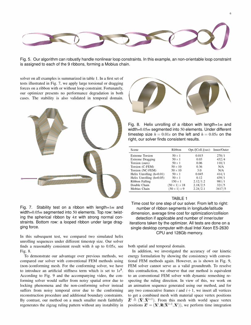
Fig. 5. Our algorithm can robustly handle nonlinear loop constraints. In this example, an non-orientable loop constraintis assigned to each of the 9 ribbons, forming a Mobius chain.

solver on all examples is summarized in table 1. In a first set oftests illustrated in Fig. 7, we apply large torsional or draggingforces on a ribbon with or without loop constraint. Fortunately,our optimizer presents no performance degradation in bothcases. The stability is also validated in temporal domain.

Fig. 7. Stability test on a ribbon with length=1m andwidth=0.05m segmented into 50 elements. Top row: twist-ing the spherical ribbon by 4π with strong normal con-straints. Bottom row: a looped ribbon under large drag-ging force.

In this subsequent test, we compared two simulated helixunrolling sequences under different timestep size. Our solverfinds a reasonably consistent result with h up to 0.05s, seeFig. 8.

To demonstrate our advantage over previous methods, wecompared our solver with conventional FEM methods using(non-)conforming mesh. For the conforming solver, we haveto introduce an artificial stiffness term which is set to 1e8.According to Fig. 9 and the accompanying video, the con-forming solver would suffer from noisy spatial error due tolocking phenomena and the non-conforming solver insteadsuffers from noisy temporal error due to the conformingreconstruction procedure and additional boundary constraints.By contrast, our method on a much smaller mesh faithfullyregenerates the zigzag ruling pattern without any instability in

Fig. 8. Helix unrolling of a ribbon with length=1m andwidth=0.05m segmented into 50 elements. Under differenttimestep size h = 0.01s on the left and h = 0.05s on theright, our solver finds consistent results.

Scene Ribbon Opt./[Coll.](sec) Inner/Outer

Extreme Torsion 50×1 0.015 270/1Extreme Dragging 50×1 0.03 432/4Torsion (ours) 50×1 0.06 110/1Torsion (C-FEM) 50×10 0.36 N/ATorsion (NC-FEM) 50×10 3.0 N/AHelix Unrolling (h=0.01) 50×1 0.045 414/1Helix Unrolling (h=0.05) 50×1 0.12 439/1Ribbon Falling 150×1 2.12/1.2 981/1Double Chain (50×1)×18 2.18/2.5 321/5Mobius Chain (50×1)×9 2.24/2.1 3417/5

TABLE 1Time cost for one step of our solver. From left to right:

number of ribbon segments in longitude/latitudedimension, average time cost for optimization/collision

detection if applicable and number of inner/outeriterations taken by the optimizer. All tests are done on asingle desktop computer with dual Intel Xeon E5-2630

CPU and 128Gb memory.

both spatial and temporal domain.In addition, we investigated the accuracy of our kinetic

energy formulation by showing the consistency with conven-tional FEM methods again. However, as is shown in Fig. 9,FEM solver cannot serve as a valid groundtruth. To resolvethis contradiction, we observe that our method is equivalentto an conventional FEM solver with dynamic remeshing re-specting the ruling direction. In view of this, we work onan animation sequence generated using our method, and forany two consecutive frames i and i+1, we insert all verticesto get a combined mesh with material space vertex positionsZi , (Xi, Xi+1). From this mesh with world space vertexpositions Zi = (Xi,R(Xi+1,Xi)), we perform time integration

7

Fig. 10. The animation of free helix unrolling with h = 0.01s. Visualization of discrepancy between Zi+1FEM (red) and Zi+1

(brown) at t = 0s,0.25s,0.5s,0.75s,1s, from left to right. For reference, Zi is also shown in green.

Fig. 9. Twisting a ribbon with length=1m and width=0.1msegmented into 50 longitude elements and 10 latitudeelements. From top to bottom: our method, FEM solver ona conforming mesh and FEM solver on a non-conformingmesh.

using FEM method on conforming mesh to predicate a newcombined mesh with world space vertex positions Zi+1

FEM,which is then compared with Zi+1 , (R(Xi,Xi+1),Xi+1). Thisessentially compares the per-frame discrepancy between ourmethod and FEM method with remeshing factored out. Theresult is visualized in Fig. 10, which validates the accuracyof our formulation. Unfortunately, such accuracy is achievedat the cost of an additional resampling operator R. There ishowever a naive simplification to our kinetic term by lumpingall the mass to the centerline, giving a simplified objectiveenergy:

f ,n

∑i=0

Mi

2

∥∥(xn+1i +yn+1

i −xni −yn

i )/2h− (xni + yn

i )/2∥∥2

+V,

which just takes the average of velocities and positions alongthe ruling direction for the centerline. Here Mi is the constantlumped mass for the ith centerline vertex. Such approximationworks well in some cases such as Fig. 10 but may lead tosevere artifact elsewhere. An extreme example is shown inFig. 11.

One major disadvantage of our algorithm is that the perfor-mance degenerates with the number of segments according toFig. 13. The bottleneck of our method is the evaluation of ∇x jand ∇y j which is quadratic in n, which can be largely removed

Fig. 11. A ribbon rotating along the centerline (no gravity).If lumped kinetic energy is used, the ribbon won’t evendeform since f = 0 is always achieved at the rest state(top). While our formulation correctly captures the trian-gular ruling pattern (middle), which finally leads to largedeformation due to centrifugal force (bottom).

using the adjoint method. But longer ribbon won’t affect thestability our method. In the falling ribbon example of Fig. 12,we used a long ribbon with 150 segments. In this case theoverhead of optimization dominates our solver pipeline.

The stability of collision and contact handling is illustratedin Fig. 12 as well. For both of these examples we used h =0.01. Under such large timestep size, our new closeness metricE is an indispensable component especially for the doubleribbon chain example. Due to the stiffness of collision forces,conventional non-rigid impact zone solver generates extremelydistorted triangles and quickly fails after the first few segmentsof the chain get in contact.

7 CONCLUSION AND DISCUSSION

In conclusion, the paper presents an configuration space thatcovers a large subset of the shape space of developable ribbon.Based on this configuration space, we develop a optimizationbased ribbon simulator with flexible user controllability androbust collision handling. Thanks to the compactness of theconfiguration space, the solver is locking free compared withprevious FEM based methods. This enables the solver highfidelity on a very small mesh. Moreover, it presents betterstability in both temporal and spatial domain over conventionalmethods [17], [6].

8

Fig. 12. Our method handles collision and contact ro-bustly. Top: A long ribbon falling on the ground. Bottom:impact of two ribbon chains with 9 ribbons each.

0

2

4

6

8

10

Time (sec)

50 100 150 200 250 300No. Segment

Fig. 13. Time cost of finding the rest shape of a mobiusband for ribbon of different length, using simple chainrule (red) or the adjoint method (blue) energy gradientevaluation.

We also noticed several drawbacks of the method. A clearproblem is that our configuration parameters are denselyrelated to vertex positions, which limits the scalability interms of both time and memory for extremely long chain.The optimizer would also require more gradient evaluationsfor longer ribbon. To alleviate this problem, it is worth ex-ploring acceleration techniques such as Newton-type optimizerwith an approximate Hessian or massive parallelism. Anothermajor drawback is that, as the width of ribbon increase, ourconfiguration space represents a smaller subspace of the trueshape space. And sometimes user may want to recover somelocal deformation. In these cases, locally deformed patches canbe reintroduced by coupling the solver to conventional FEMmethods or model reduction techniques such as [30].

REFERENCES

[1] M. P. Do Carmo and M. P. Do Carmo, Differential geometry of curvesand surfaces. Prentice-hall Englewood Cliffs, 1976, vol. 2.

[2] P. Bo and W. Wang, “Geodesic-controlled developable surfaces formodeling paper bending,” Computer Graphics Forum, vol. 26, no. 3,pp. 365–374, 2007. [Online]. Available: http://dx.doi.org/10.1111/j.1467-8659.2007.01059.x

[3] J. Solomon, E. Vouga, M. Wardetzky, and E. Grinspun, “Flexibledevelopable surfaces,” Computer Graphics Forum, vol. 31, no. 5,pp. 1567–1576, 2012. [Online]. Available: http://dx.doi.org/10.1111/j.1467-8659.2012.03162.x

[4] E. Grinspun, A. N. Hirani, M. Desbrun, and P. Schroder, “Discreteshells,” in Proceedings of the 2003 ACM SIGGRAPH/Eurographicssymposium on Computer animation. Eurographics Association, 2003,pp. 62–67.

[5] E. English and R. Bridson, “Animating developable surfaces usingnonconforming elements,” ACM Transaction on Graphics, 2008.

[6] ——, “Animating developable surfaces using nonconforming elements,”in ACM Transactions on Graphics (TOG), vol. 27, no. 3. ACM, 2008,p. 66.

[7] J. Spillmann and M. Teschner, “Corde: Cosserat rod elements for thedynamic simulation of one-dimensional elastic objects,” in In Proc. ACMSIGGRAPH/Eurographics Symposium on Computer Animation, 2007,pp. 63–72.

[8] F. Bertails, B. Audoly, M.-P. Cani, B. Querleux, F. Leroy, and J.-L.Leveque, “Super-helices for predicting the dynamics of natural hair,” inACM Transactions on Graphics (TOG), vol. 25, no. 3. ACM, 2006,pp. 1180–1187.

[9] R. Casati and F. Bertails-Descoubes, “Super space clothoids,” ACMTransactions on Graphics (TOG), vol. 32, no. 4, p. 48, 2013.

[10] E. Cosserat and F. Cosserat, “Theorie des corps deformables,” Paris,1909.

[11] S. Javdani, S. Tandon, J. Tang, J. F. O’Brien, and P. Abbeel, “Modelingand perception of deformable one-dimensional objects,” in Robotics andAutomation (ICRA), 2011 IEEE International Conference on. IEEE,2011, pp. 1607–1614.

[12] D. K. Pai, “Strands: Interactive simulation of thin solids using cosseratmodels,” Computer Graphics Forum, vol. 21, no. 3, pp. 347–352, 2002.[Online]. Available: http://dx.doi.org/10.1111/1467-8659.00594

[13] J. Spillmann and M. Teschner, “C o r d e: Cosserat rod elements for thedynamic simulation of one-dimensional elastic objects,” in Proceedingsof the 2007 ACM SIGGRAPH/Eurographics symposium on Computeranimation. Eurographics Association, 2007, pp. 63–72.

[14] M. Bergou, M. Wardetzky, S. Robinson, B. Audoly, and E. Grinspun,“Discrete elastic rods,” in ACM Transactions on Graphics (TOG),vol. 27, no. 3. ACM, 2008, p. 63.

[15] F. Bertails, “Linear time super-helices,” in Computer graphics forum,vol. 28, no. 2. Wiley Online Library, 2009, pp. 417–426.

[16] P. G. Ciarlet, Theory of shells. Elsevier, 2000.[17] E. Grinspun, A. N. Hirani, M. Desbrun, and P. Schroder, “Discrete

shells,” in Proceedings of the 2003 ACM SIGGRAPH/Eurographicssymposium on Computer animation. Eurographics Association, 2003,pp. 62–67.

[18] R. Bridson, S. Marino, and R. Fedkiw, “Simulation of clothingwith folds and wrinkles,” in Proceedings of the 2003 ACM SIG-GRAPH/Eurographics symposium on Computer animation. Eurograph-ics Association, 2003, pp. 28–36.

[19] R. Goldenthal, D. Harmon, R. Fattal, M. Bercovier, and E. Grin-spun, “Efficient simulation of inextensible cloth,” ACM Transactions onGraphics (TOG), vol. 26, no. 3, p. 49, 2007.

[20] M. Wardetzky, M. Bergou, D. Harmon, D. Zorin, and E. Grinspun,“Discrete quadratic curvature energies,” Computer Aided GeometricDesign, vol. 24, no. 8, pp. 499–518, 2007.

[21] P. Bo and W. Wang, “Geodesic-controlled developable surfaces formodeling paper bending,” in Computer Graphics Forum, vol. 26, no. 3.Wiley Online Library, 2007, pp. 365–374.

[22] Y. Liu, H. Pottmann, J. Wallner, Y.-L. Yang, and W. Wang, “Geometricmodeling with conical meshes and developable surfaces,” in ACMTransactions on Graphics (TOG), vol. 25, no. 3. ACM, 2006, pp.681–689.

[23] S. Martin, B. Thomaszewski, E. Grinspun, and M. Gross, “Example-based elastic materials,” in ACM Transactions on Graphics (TOG),vol. 30, no. 4. ACM, 2011, p. 72.

[24] D. Cohen-Steiner and J.-M. Morvan, “Restricted delaunay triangulationsand normal cycle,” in Proceedings of the nineteenth annual symposiumon Computational geometry. ACM, 2003, pp. 312–321.

[25] R. Narain, A. Samii, and J. F. O’Brien, “Adaptive anisotropic remeshingfor cloth simulation,” ACM Transactions on Graphics (TOG), vol. 31,no. 6, p. 152, 2012.

9

[26] R. H. Byrd, P. Lu, J. Nocedal, and C. Zhu, “A limited memory algo-rithm for bound constrained optimization,” SIAM Journal on ScientificComputing, vol. 16, no. 5, pp. 1190–1208, 1995.

[27] J. Nocedal and S. J. Wright, “Numerical optimization, second edition,”Numerical optimization, pp. 497–528, 2006.

[28] R. Bridson, R. Fedkiw, and J. Anderson, “Robust treatment of collisions,contact and friction for cloth animation,” in ACM Transactions onGraphics (ToG), vol. 21, no. 3. ACM, 2002, pp. 594–603.

[29] D. Harmon, E. Vouga, R. Tamstorf, and E. Grinspun, “Robust treatmentof simultaneous collisions,” in ACM Transactions on Graphics (TOG),vol. 27, no. 3. ACM, 2008, p. 23.

[30] D. Harmon and D. Zorin, “Subspace integration with local deforma-tions,” ACM Transactions on Graphics (TOG), vol. 32, no. 4, p. 107,2013.

APPENDIX AEXPLICIT FORMULA FOR x j AND ∇x j

Since Tk for 1≤ k < n is just rigid rotation, they have simpleanalytical form:

Tk =

cos(ψk)+c2k

c2k+1

ck−ckcos(ψk)

c2k+1

−sin(ψk)√c2

k+1

kl−klcos(ψk)

n(c2k+1)

ck−ckcos(ψk)

c2k+1

1+c2kcos(ψk)

c2k+1

cksin(ψk)√c2

k+1

ckklcos(ψk)−ckkl

n√

c2k+1

sin(ψk)√c2

k+1

−cksin(ψk)√c2

k+1cos(ψk)

−klsin(ψk)

n√

c2k+1

0 0 0 1

,

whose partial derivatives ∂Tk/∂ck and ∂Tk/∂wk can be foundusing a symbolic software. We omit these here to save space.And for the global rigid transformation, we have:

∂T0

∂wk=

(∂expw

∂wk0

0 1

)∂T0

∂ tk=

(0 ek0 1

),

where ∂expw/∂wk can be found using the Rodriguez’s for-mula. Now ∇x j can be founding using simply chain rule:

∂x j

∂ck=

[Π

k−1i=0 Ti

]∂Tk

∂ck

[Π

ji=k+1Ti

]x j +

[Π

ji=0Ti

]∂ x j

∂ck.

∂x j

∂ψk=

[Π

k−1i=0 Ti

]∂Tk

∂ψk

[Π

ji=k+1Ti

]x j

∂x j

∂wk=

∂T0

∂wk

[Π

ji=1Ti

]x j

∂x j

∂ tk=

∂T0

∂ tk

[Π

ji=1Ti

]x j.

APPENDIX BTHE MASS MATRIX

Without loss of generality, we use linear shape function foreach quad element. In this case, element Ei would contributea 12×12 mass block of the following form:

Mi =

−∆cnw2+4lw

36nlw

18n−∆cnw2+4lw

72nlw

36nlw

18n∆cnw2+4lw

36nlw

36n∆cnw2+4lw

72n−∆cnw2+4lw

72nlw

36n−∆cnw2+4lw

36nlw

18nlw

36n∆cnw2+4lw

72nlw

18n∆cnw2+4lw

36n

⊗ Id3×3,

where ∆c = ci+1− ci.

APPENDIX CADJOINT MODE GRADIENT EVALUATION

In order to evaluate d fd<c,ψ> , we start from the chain rule:

d fd< c,ψ >

=∂ f∂X

∂X∂< c,ψ >

+∂ f∂N

∂N∂< c,ψ >

+∂ f

∂< c,ψ >,

where the first two terms can then be evaluated in an adjointmode by exploiting the special structure of equation 2 andequation 3, which is composed of two passes as illustratedin Algorithm 3. In this way, the algorithmic complexity isreduced from O(n2) to O(n).

Algorithm 3 Adjoint Gradient EvaluationInput: < c,ψ >Output: d f

d<c,ψ>

1: T = Id . forward pass2: for j = 0, · · · ,n do3: T = TT j4: x j = Tx j5: y j = Ty j6: end for7: evaluate f , ∂ f

∂X ,∂ f∂N ,

∂ f∂<c,ψ>

8: d fd<c,ψ> = ∂ f

∂<c,ψ> . backward pass9: A = 0 . adjoint variable

10: for j = n, · · · ,0 do11: d f

dc j= d f

dc j+(T ∂ x j

∂c j)T ∂ f

∂x j+(T ∂ y j

∂c j)T ∂ f

∂y j

12: T = TT−1j

13: A = T−Tj ATT

j+1

14: A = A+TT ( ∂ f∂x j

xTj +

∂ f∂y j

yTj +

∂ f∂n j

nT )

15: d fdc j

= d fdc j

+A: ∂T j∂c j

16: d fdψ j

= d fdψ j

+A: ∂T j∂ψ j

17: end for