Modelling Deforming Interfaces using Level Sets

byHans Mühlhaus, Laurent Bourgouin and

Lutz Gross

The Australian Computational Earth Systems Simulator

(ACcESS)

Overview

Introducing Example What’s needed to model interfaces

• Constitutive models• Surface tracking, level set, stress advection

EScript & Finley Separation of Physics from Linear Algebra and Parallel Computing

Applications• Advection, upwinding, implicit vs. explicit• Lava dome simulation , Subduction, Rayleigh-Taylor Instabilities

Moving Interface: a 1D Example

2xh

0arg

0

ifel

ifsmall

02,2, vt

v2

x1

x2h large

small

We define: so that

Update: Note that:

2tvttt Time integration:

12,

Governing equations

0))(( ,,,

izijlkjkiljlik gpv

ij

jjjjtp kTTvTc ,,,, )()(

))()(1( 00

00 CCTT

Temperature and concentration dependence of density:

Heat Equation

Stress Equilibrium

Concentration advection:

0,, iit CvC

else

materialheavierinC

0

1

Example for Rayleigh – Taylor Instabilities using level sets: Mantle Plumes

The General Case

• Implicit representation of the interface by the zero level set of a smooth function φ

• φ is usually chosen as a “signed” distance function ( )

• At each time step, φ is updated solving the (hyperbolic) advection equation:

0,, kkt v

1

Problems……

1

x

TT ii

1

1. Symmetric difference expressions like

(symm.) (non-symm.)

don’t work well in hyperbolic problems (upwinding etc!)

2. Inhomogeneous velocity field causes lossof distance function property ( ) of

x

TT ii

2

11

Problems……(cont.)

),(

)23262

(

11

111111

,,,

1

1

ii

iiiiiiiiiiii

x

x

x

x

x

xxx

wwO

h

vvh

h

vvh

hhvw

wdxvwdxvv

i

i

i

i

i

hhvv

ii

xx i2

11

,

1. Symmetric difference expressions don’t work well in hyperbolic problems (upwinding!)

1. Upwinding

If v is constant:

Problems……

hhv

hhv

hhv

iiiiiii 11111

2

2

2

This can be transformed into a non-symmetric expression by adding….

We expect that the FE approx. of the PDE:

02 ,,, xxxt

hvv

is better conditioned than the original Hyperbolic problem

Generalisations…..

)2

32

2

tO(+t

Δt+

tΔt+=

t2tttt

.2

hotx

vvx

Δt+

xvΔt=

j

t

jii

2

j

t

jttt

j

t

jt

t+t

xv

Δt=

2

2

Taylor-Galerkin:

2-step alternative to Taylor-Galerkin upwinding (very effective in the presence of diffusionterms….):

j

tt

jttt

xvΔt=

2

2 Gaussians

1 Gaussian

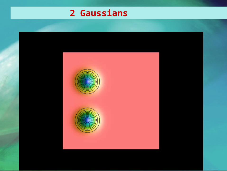
The Level Set Method: Solving the advection equation

• Explicit

• Implicit

• Taylor Galerkin

)( ,tjj

ttt vt

tttjj

tt vt )( ,,

ktjjk

tjj

ttt vvt

vt ,,

2

,, )(2

)(

Test:A Gaussian is advected in a constant 1D velocity field.

Formulation

Finley PDE:

jijijijjkijkjkijkjlkijkl XYvDvCvBvA ,,,,, )()(

Example : Momentum and Heat equation

0))

2(

0)(

,,,

/1

)(

,,,

,

jti

X

ijijtj

C

j

Y

t

tD

tt

Y

i

p

ijlk

A

ijkl

Tvvt

Tvt

T

t

T

RaTgpvE

jj

i

ijX

jijijkl

Software can be downloaded fromwww.esscc.uq.edu.au, contact Ken Steube (esys@access.edu.au) If you need instructions re libraries etc

LinearPDE class

General form (as relevant here):

Y=Du+uAj,i,ij

duy=uAn i,ijj

PDE:

natural boundary condition

g=yη=d

f=Yω=Dκδ=A ijij

Kronecker symbol: δij=0 for i=j and 0 otherwise

f=κuωui,i,

Helmholtz Class in mytools.py

from esys.linearPDEs import LinearPDEimport numarrayclass Helmholtz(LinearPDE): def setValue(self,kappa,omega,f,eta,g): ndim=self.getDim() # spatial dimension kronecker=numarray.identity(ndim) self._setValue(A=kappa*kronecker,\ D=omega,Y=f,d=eta,\

y=g)

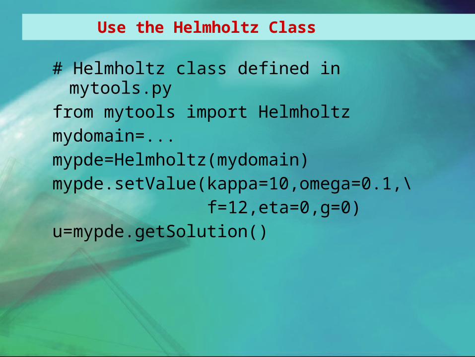
Use the Helmholtz Class

# Helmholtz class defined in mytools.py

from mytools import Helmholtzmydomain=...mypde=Helmholtz(mydomain)mypde.setValue(kappa=10,omega=0.1,\ f=12,eta=0,g=0)u=mypde.getSolution()

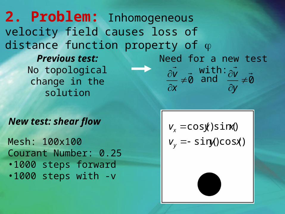
2. Problem: Inhomogeneous velocity field causes loss of distance function property of

Previous test:No topological change in the

solution

Need for a new test with:

0x

v0

y

vand

New test: shear flow

)cos()sin(

)sin()cos(

xyv

xyv

y

x

Mesh: 100x100Courant Number: 0.25•1000 steps forward•1000 steps with -v

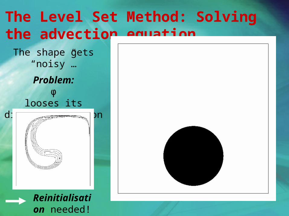
The Level Set Method: Solving the advection equation The shape gets “noisy”…

Problem:φ

looses its distance function property

Reinitialisation needed!

The Level Set Method: Reinitialisation Idea:

Rebuild a “signed” distance function ψ from the distorted function φ

Requirements:• The interface must not be changed

• ψ must represent a distance function

Solution:Solve to steady state the equation:

Rewritten as:

00

1

)1)(( 0

sign

)( 0

sign

w

wwith

Interpretation:The “distance information” is carried by w, a unit vector

pointing away from the interface.

Remarks on re-initialisation…..

• During iteration (pseudo time integration) the vector w is established once and then kept constant

• In the explicit solution of the advection problem for we found that only alumped mass matrix discretisation works

The Level Set Method: Reinitialisation (2/3)

1D2D

3D

The Level Set Method: Reinitialisation

Same test as before, with

reinitialisation

Level set cont. : Merger of small and large bubbles

4

222

411

10

10,1800

10,3160

11,

121 )()( jjjjijij nnn

0

1 /

gradgradn

Parameters:

Surface tension:

10

1121 )()( nnnσσ divnT

Calculation, includes inertia, CourantNumber=0.5, msh:30 by 458 node quad’s

Level set cont. : Calculation of curvature for C_0 continuity

grad

gradN Ndiv

RRS

11

jijijijjkijkjkijkjlkijkl XYvDvCvBvA ,,,,, )()(

Projection:

and

Representation of surface tension b.c. as volume force:

NY )11

(2

2

RRl

en

s

l

x

T

n

l smoothing length, related to the element size

=distance in the direction of the normal of

nx0 at

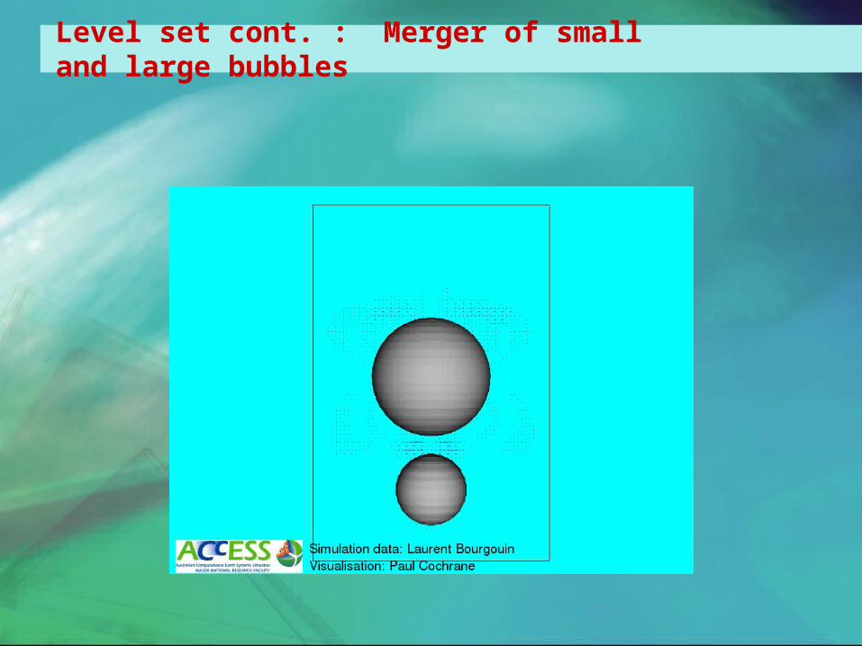
Level set cont. : Merger of small and large bubbles

Surface Tension: Benchmark

Level set: Surface membrane shell, surface tension

R

n

R

np

s

ssn ),(,, zrjinnp jiijn where

Tss nnn )11

(RR

nps

Tn Inserting yields

whereTnpR 2 at equilibrium.

Collapsing Cylinder

Lava Dome

Remarks

• Escript & Finley: Rapid development of simulation software; parallelised assembly and solution phase; separation of physics from linear algebra

• Level set modelling of interfaces: distance function property crucial

• Modelling of surface tension; example of higher order b.c.’s• Upwinding strategy dependent on element

type• Re-initialisation strategy has an (undesirable)

element of mystique…..