Modelling Australia's imports of goods and services€¦ · Web viewWe build on earlier demand...

MODELLING AUSTRALIA’S IMPORTS OF GOODS AND SERVICES

Alexander Beames and Michael Kouparitsas1

Treasury Working Paper2

2015-02Date created: June 2015Date modified: June 2015

1 Macroeconomic Modelling and Policy Division, Macroeconomic Group, The Treasury, Langton Crescent, Parkes ACT 2600, Australia. Correspondence: [email protected]. We thank Michal Krolikowski, Linden Luo, Sarah Brown and participants at the Macroeconomic Theory and Application Seminar for comments and suggestions on an earlier draft.

2 The views expressed in this paper are those of the authors and do not necessarily reflect those of The Australian Treasury or the Australian Government.

Odd landscape headerDED ModelDocumentation

mailto:[email protected]

© Commonwealth of Australia 2015

ISBN 978-1-925220-56-8

This publication is available for your use under a Creative Commons BY Attribution 3.0 Australia licence, with the exception of the Commonwealth Coat of Arms, the Treasury logo, photographs, images, signatures and where otherwise stated. The full licence terms are available from http://creativecommons.org/licenses/by/3.0/au/legalcode .

Use of Treasury material under a Creative Commons BY Attribution 3.0 Australia licence requires you to attribute the work (but not in any way that suggests that the Treasury endorses you or your use of the work).

Treasury material used 'as supplied'.

Provided you have not modified or transformed Treasury material in any way including, for example, by changing the Treasury text; calculating percentage changes; graphing or charting data; or deriving new statistics from published Treasury statistics — then Treasury prefers the following attribution:

Source: The Australian Government the Treasury.

Derivative material

If you have modified or transformed Treasury material, or derived new material from those of the Treasury in any way, then Treasury prefers the following attribution:

Based on The Australian Government the Treasury data.

Use of the Coat of ArmsThe terms under which the Coat of Arms can be used are set out on the It’s an Honour website (see www.itsanhonour.gov.au)

Other usesEnquiries regarding this licence and any other use of this document are welcome at:

ManagerMedia UnitThe TreasuryLangton Crescent Parkes ACT 2600Email: [email protected]


mailto:[email protected]

http://www.itsanhonour.gov.au/

http://creativecommons.org/licenses/by/3.0/au/deed.en

http://creativecommons.org/licenses/by/3.0/au/legalcode

http://creativecommons.org/licenses/by/3.0/au/deed.en

Modelling Australia’s imports of goods and servicesAlexander Beames and Michael Kouparitsas2015-02June 2015

ABSTRACT

This paper adds to the relatively scant Australian literature on modelling the demand and supply of Australian imports. We build on earlier demand modelling by deriving conditional import demand relationships via representative household/firm-level utility-maximisation/cost-minimisation problems, which explicitly assume households/firms have both a taste for variety and rival sources of supply. Our estimates of disaggregated price elasticities are consistent with earlier studies in finding relatively low substitutability between imported and domestically produced varieties. Our derivation of the long-run supply framework also adds to the existing literature by explaining why it is necessary for researchers to employ trade-weighted foreign prices in place of individual country prices and providing conditions under which this approach is consistent with the underlying theory. We find that the extent of the foreign cost pass-through to import prices depends critically on the choice of foreign cost variable.

JEL Classification Numbers: F14, F17, C22Keywords: Import prices, price elasticity of imports, income elasticity of imports

Alexander Beames and Michael KouparitsasMacroeconomic Modelling and Policy DivisionMacroeconomic GroupThe TreasuryLangton CrescentParkes ACT 2600


1. INTRODUCTION

Imports play a critical role in fostering long-run growth and smoothing business cycles of small open economies, including Australia. International trading characteristics of small open economies vary greatly so it not surprising then that the bulk of the research on modelling demand and supply of imports concentrates on country-specific studies of small open economies. As demonstrated by Goldstein and Khan (1985), the income and price elasticities of demand and supply generated by this literature have been applied to a host of real world macroeconomic policy issues faced by small open economies, including the international transmission of foreign demand/supply shocks.

This paper adds to the relatively scant Australian literature by modelling both the demand and supply of Australian imports. We build on earlier demand modelling by Wilkinson (1992); Jilek, Johnson and Taplin (1993); and Dwyer and Kent (1993) by deriving conditional import demand relationships via representative household/firm-level utility-maximisation/cost-minimisation problems, which explicitly assume households/firms have both a taste for variety and rival sources of supply. This long-run theoretical framework is augmented by cyclical explanatory variables to form empirical error correction models (that is, short-run demand models) which are then estimated using standard econometric methods. Our estimates of disaggregated import price elasticities are consistent with earlier work by Dwyer and Kent (1993) in finding relatively low substitutability between imported and domestically produced varieties. The main implication of this finding is that income effects dominate the substitution effects resulting from a relative price movement, so other things being equal a fall in import prices leads to a rise in the demand for both imports and rival domestically produced goods.

The theoretical framework underpinning our modelling of the supply of imports is motivated by previous Australian research undertaken by Dwyer and Lam (1994), and updated work by Chung, Kohler and Lewis (2011), which suggests Australian households/firms are price takers facing an import price equal to the exchange rate adjusted foreign cost. We add to this literature by explaining why it is necessary for researchers to employ trade-weighted foreign prices in place of individual country prices and provide conditions under which this approach is consistent with the underlying imports supply theory. Again, the long-run theoretical framework is augmented by cyclical explanatory variables to form empirical error correction models (that is, short-run supply models) which are estimated using standard econometric methods. We find that the extent of the pass-through of changes to foreign costs to import prices depends critically on the choice of foreign cost variable. Our analysis relies on a trade-weighted index of foreign consumer prices which displays far less pass-through than previous Australian studies which rely on indices of foreign export prices.

The remainder of this paper is organised as follows: Section 2 derives the theoretical long-run import demand and supply relationships; Section 3 describes the data used in estimating import demand and supply; Section 4 provides details of the econometric method and reports parameter estimates; and Section 5 summarises the analysis.

1


2. THEORY

Long-run demand for imports

Consider a representative consumer living in country i who solves a nested utility maximisation problem. At the top of the nest is the choice between different types of consumption goods. Assuming the consumer’s preferences are captured by Dixit and Stiglitz (1977) preferences (that is, a constant elasticity of substitution utility function), the problem can be summarised by the following:

11\* MERGEFORMAT ()

subject to:

22\* MERGEFORMAT ()

where cit is the ideal/aggregate consumption level, pcit is the ideal/aggregate consumption price, q is the number of varieties, cit

k the consumption level of good k, pcitk the price of consumption good k, i

k is the good k weighting parameter and is the elasticity of substitution between varieties.

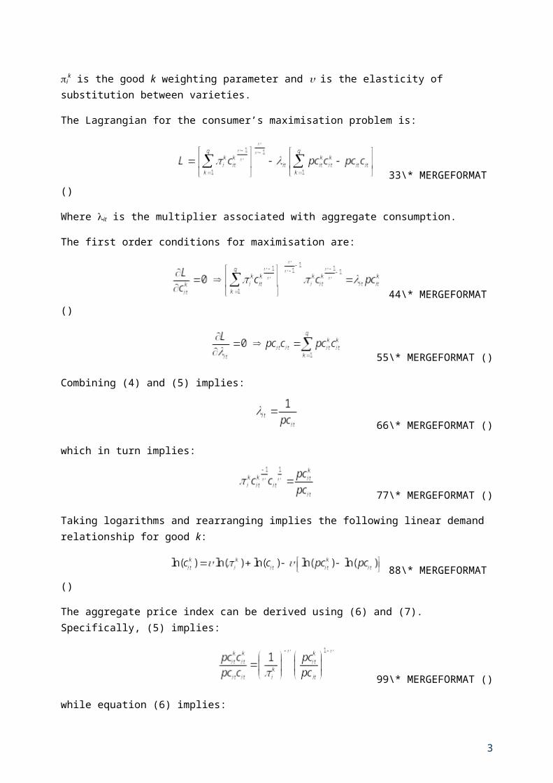
The Lagrangian for the consumer’s maximisation problem is:

33\* MERGEFORMAT ()

Where it is the multiplier associated with aggregate consumption.

The first order conditions for maximisation are:

44\* MERGEFORMAT ()

55\* MERGEFORMAT ()

Combining (4) and (5) implies:

66\* MERGEFORMAT ()

which in turn implies:

2

77\* MERGEFORMAT ()

Taking logarithms and rearranging implies the following linear demand relationship for good k:

88\* MERGEFORMAT ()

The aggregate price index can be derived using (6) and (7). Specifically, (5) implies:

99\* MERGEFORMAT ()

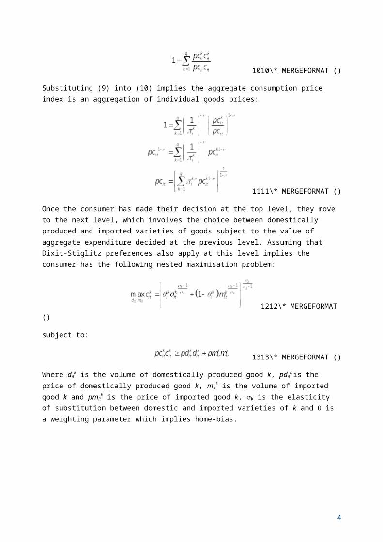
while equation (6) implies:

1010\* MERGEFORMAT ()

Substituting (9) into (10) implies the aggregate consumption price index is an aggregation of individual goods prices:


Once the consumer has made their decision at the top level, they move to the next level, which involves the choice between domestically produced and imported varieties of goods subject to the value of aggregate expenditure decided at the previous level. Assuming that Dixit-Stiglitz preferences also apply at this level implies the consumer has the following nested maximisation problem:


subject to:


Where ditk is the volume of domestically produced good k, pdit

k is the price of domestically produced good k, mit

k is the volume of imported good k and pmitk is the price of imported good k, k is the

3

elasticity of substitution between domestic and imported varieties of k and is a weighting parameter which implies home-bias.

4

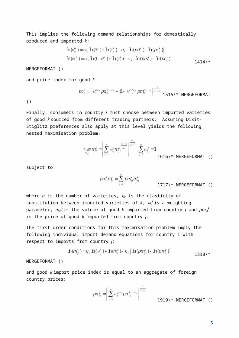
This implies the following demand relationships for domestically produced and imported k:


and price index for good k:


Finally, consumers in country i must choose between imported varieties of good k sourced from different trading partners. Assuming Dixit-Stiglitz preferences also apply at this level yields the following nested maximisation problem:


subject to:


where n is the number of varieties, k is the elasticity of substitution between imported varieties of k, ij

k is a weighting parameter, mijtk is the volume of good k imported from country j and pmijt

k is the price of good k imported from country j.

The first order conditions for this maximisation problem imply the following individual import demand equations for country i with respect to imports from country j:


and good k import price index is equal to an aggregate of foreign country prices:


Long-run supply of imports

Following previous Australian research on exchange rate and foreign cost pass-through by Dwyer and Lam (1994) country i is assumed to be a small open economy that has a negligible impact on world prices. As such, the supply curve faced by country i for good k produced by country j is assumed to be perfectly elastic, with the good k import price simply the exchange rate adjusted country j consumption good price for good k:


5

where pcjtk is the price of consumption of good k in country j and eijt is the country i-country j exchange

rate in terms of country i currency.

The lack of country specific trade flow data means that imports can only be modelled at the level of a good described by equation (14). A key challenge for researchers that results from this is the need to estimate an aggregate import price index without knowledge of the elasticity of substitution for foreign varieties. This paper responds to this challenge by approximating the aggregate import price index described by equation (19) using a linear approximation. In particular, aggregate import price indexes are estimated using a first-order Taylor series approximation of (19) evaluated at the previous period’s price and quantity bundle:


Dividing through by pmitk on both sides implies:


Equation (9) implies:


where sijtk is the time t import share of country j’s good. Substituting (23) into (22) and recognising

ln(1+) ≈ for small , implies the following approximate aggregate import price index for good k:


Substituting (20) into (24) implies:

6


7

This expression can be further simplified by assuming there exists a trade-weighted foreign goods price index pcijt

k* such that:


and a trade-weighted exchange rate index eit such that:


Assuming without loss of generality that base period prices are one implies:


In words, the aggregate import price index for good k is equal to the trade-weighted foreign consumption price index for good k and the trade-weighted exchange rate. This is the trade-weighted analogue of (20).

3. DATA

Imports of goods and services

Australian imports include both goods and services. The Australian Bureau of Statistics (2011) defines goods to be physical, produced items over which ownership rights can be established and whose economic ownership can be passed from one institutional unit to another by engaging in transactions. They may be used to satisfy final demand or used as an intermediate good in the production of other goods or services. In contrast, services are the result of a production activity that changes the conditions of the consuming units, or facilitates the exchange of products or financial assets. Services are not generally separate items over which ownership rights can be established and cannot generally be separated from their production.

The Australian Bureau of Statistics (ABS) publishes import volumes and import prices at the quarterly frequency on a seasonally adjusted basis in the Balance of Payments and International Investment Position (ABS Cat. 5302.0). According to these data, the share of imports accounted for by goods has risen slightly over the past 30 years, with goods accounting for around 77 per cent of the total imports in 1985 and around 80 per cent in 2014 (see Chart 1).

8

Chart 1: Ratio of goods and service imports to total imports value

Source: Authors’ calculations based on ABS Cat 5302.0.

Imports of goods

Australian researchers dating back to the National Income Forecasting (NIF) project of the 1970s (see Caton and Johnston, 1975, for details) and more recently, Wilkinson (1992) and Jilek, Johnson and Taplin (1993) have limited their analysis to modelling aggregate ‘endogenous imports’. These earlier studies classified endogenous imports as the residual of total goods imports less “exogenous imports”, where the latter includes civil aircraft; confidentialised items; goods procured in ports by carriers; and non-monetary gold. This is a useful distinction for modelling because exogenous imports tend to be lumpy or irregular items that do not lend themselves to systematic modelling.

More recently, Australian Bureau of Statistics (2012) noted that imported structures, such as Liquefied Natural Gas (LNG) processing plants were to be classified as engineering construction. This is at odds with the greater part of capital goods imports which tend to be machinery and equipment, so in keeping with the endogenous/exogenous distinction these goods are classified as exogenous. In practical terms this requires the ‘not elsewhere specified (nes)’ category of the capital goods imports to be assigned to the exogenous category.

Total endogenous goods imports accounted for around 95 per cent of the total value of goods imports in 1985 and around 90 per cent in 2014, with most of the decline due to the growth of exogenous capital imports relating to LNG processing plants (see Chart 2).

9

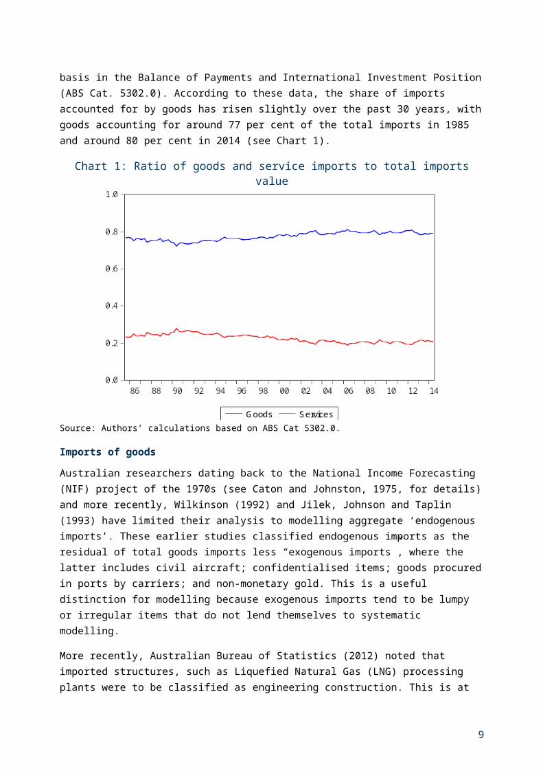
Chart 2: Ratio of total endogenous goods to total goods value


We go a step further in this paper by following Dwyer and Kent (1994) in modelling major sub-components of imports of endogenous goods. The major sub-categories of endogenous imports we analyse are: consumption goods; capital goods; and intermediate and other goods. This more general approach allows these components to have different income and price elasticities of demand.

Chart 3: Ratio of endogenous goods components to total endogenous goods value


10

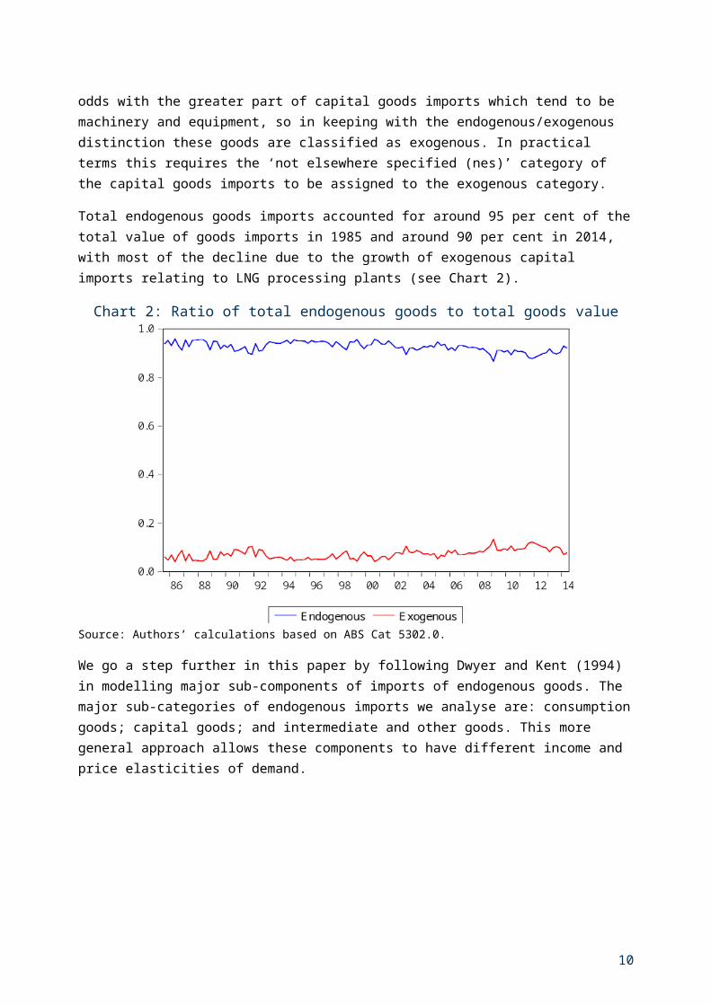
Chart 3 shows that intermediate and other goods are the largest endogenous subcategory, accounting for 55 per cent of the total value of endogenous imports in 1985 and around 48 per cent in 2014. The steady decline in the share of intermediate and other goods has largely been offset by a rising share of consumption goods. Consumption have risen from around 25 per cent of the value of endogenous imports in 1985 to around 33 per cent in 2014, while capital goods have accounted for a roughly constant share of around 19 per cent.

Imports of services

Service imports cover a range of activities: manufacturing services on physical inputs owned by others; maintenance and repair services; transportation services, travel services; and other services. Previous Treasury modelling undertaken as part of the NIF project explained imports at a disaggregated level. The analysis presented here is limited to aggregate services, which implicitly assumes they are homogenous activities. We leave it to our future research to explore the appropriateness of this assumption.

Import penetration versus relative import prices

The theory outlined above predicts that if there is substitution between domestically produced and imported goods/services (that is, > 0), then the import penetration ratio of these goods/services (that is, the ratio of the volume of imports to the volume of total expenditure) should be inversely related to their respective relative import price (that is, the ratio of the import price to the price of total expenditure) multiplied by their corresponding elasticity of substitution. Before we can explore this relationship in the data we need to define the aggregate expenditure basket for each of the import components. We assume that: the consumption expenditure aggregate is household final consumption expenditure less expenditure on rental services; the capital expenditure aggregate is total gross fixed capital expenditure on machinery and equipment less expenditure on lumpy investment items; the intermediate expenditure aggregate is total gross national expenditure less expenditure on rental services and lumpy investment items; and the services expenditure aggregate is total gross national expenditure.

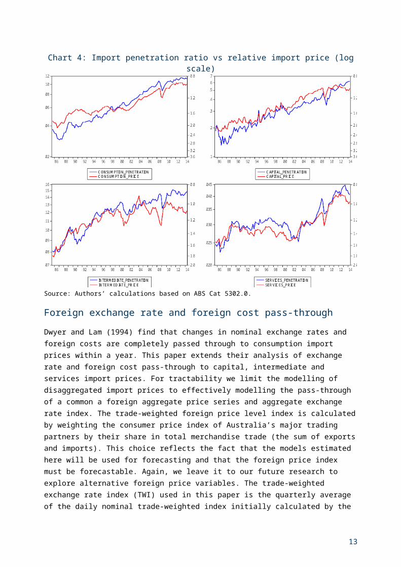
Chart 4 plots the import penetration ratio of each category (left hand axis using a log scale axis) and the relative import price of each category (right hand axis using an inverted log scale). Note that while the derivation of the theoretical model ignored taxes, the relative import prices reported here are inclusive of taxes on imports and taxes on aggregate expenditure. Dwyer and Kent (1993) find that the trend rise in import penetration can partly be explained by the reduction in protection and increased trade openness, suggesting a role for trade policy in explaining import volumes. The data show that relative import price has fallen over the sample for all four import categories. Consistent with the theory derived above, these data show that the import penetration ratios of all four import categories have increased over the same period. For example, the import penetration ratio of capital goods increased from 15 per cent in 1985 to 60 per cent in 2013, while the relative price of capital goods has fallen to a level at the end of the sample (to around one) that is roughly half its starting value (of around two).

11

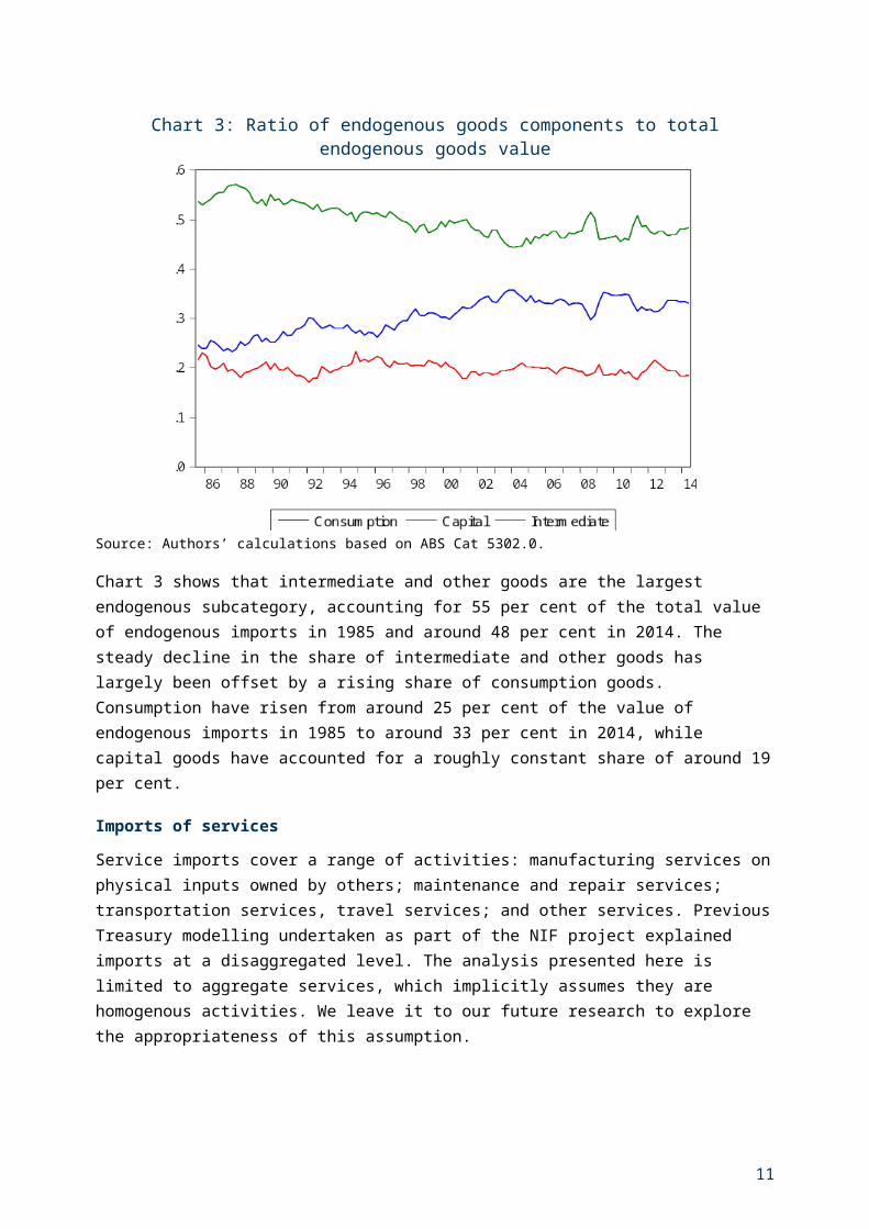
Chart 4: Import penetration ratio vs relative import price (log scale)


Foreign exchange rate and foreign cost pass-through

Dwyer and Lam (1994) find that changes in nominal exchange rates and foreign costs are completely passed through to consumption import prices within a year. This paper extends their analysis of exchange rate and foreign cost pass-through to capital, intermediate and services import prices. For tractability we limit the modelling of disaggregated import prices to effectively modelling the pass-through of a common a foreign aggregate price series and aggregate exchange rate index. The trade-weighted foreign price level index is calculated by weighting the consumer price index of Australia’s major trading partners by their share in total merchandise trade (the sum of exports and imports). This choice reflects the fact that the models estimated here will be used for forecasting and that the foreign price index must be forecastable. Again, we leave it to our future research to explore alternative foreign price variables. The trade-weighted exchange rate index (TWI) used in this paper is the quarterly average of the daily nominal trade-weighted index initially calculated by the Reserve Bank of Australia (see, Becker and Davies, 2002, for further details), which is published on a quarterly basis by the ABS (ABS Cat. 5302.0.).

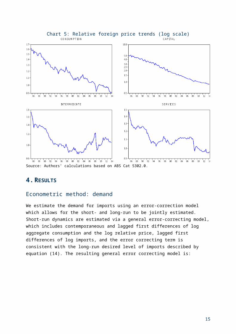
Chart 5 plots the ratio of import prices (adjusted by the TWI) to the trade-weighted foreign goods price. In contrast to Dwyer and Lam (1994), we find significant deviations from complete exchange rate and foreign cost pass-through, with all relative foreign prices displaying a downward trend from 1985 to 2014. The relative price of capital goods has the largest decline over the sample, followed by consumption and intermediate goods prices, while services prices declined over the early part of the sample and has remained roughly constant from there on.

12

One possible explanation for the vastly different trend results reported in Dwyer and Lam (1994) is the introduction of quality adjustments used by the ABS when measuring constant price volumes and their associated prices.

Goods imports tend to be durable goods, while aggregate consumption is skewed towards nondurable goods and services, which suggests that the observed trend decline of relative foreign prices is largely a by-product of the fact that the numerator is a durable good price and the denominator is an aggregate consumption good price, which includes both durable and non-durable goods. If the experience of foreign countries is similar to Australia, we would expect the relative price of durables to non-durables to fall over time. This implies our aggregate consumption goods index will overstate the true foreign goods price.

Chart 5: Relative foreign price trends (log scale)


4. RESULTS

Econometric method: demand

We estimate the demand for imports using an error-correction model which allows for the short- and long-run to be jointly estimated. Short-run dynamics are estimated via a general error-correcting model, which includes contemporaneous and lagged first differences of log aggregate consumption and the log relative price, lagged first differences of log imports, and the error correcting term is consistent with the long-run desired level of imports described by equation (14). The resulting general error correcting model is:

13


where: is a constant; is the coefficient on a linear time trend;i captures permanent level shifts; i

captures permanent slope shifts; Di denotes a dummy variable that is 0 for time periods less than i and one otherwise; t is a linear time trend; and ti is the value of the linear time trend at time i; the speed at which actual imports approaches its long-run level is determined by -1 < < 0; l captures short-run outliers; Dl denotes a dummy variable that is one at time l and 0 otherwise; and t is an error term, which is assumed to be distributed with a mean of zero and constant variance.

Estimation results: demand

Table 1 reports the estimation results for the import demand (or import volume) equations. The long-run elasticity of substitution between domestic and imported varieties of consumption, capital and intermediate goods ranges between 0.4 and 0.6. This suggests that domestic and imported varieties of these categories of imports are gross complements, which means a rise in the price of either the domestic or imported good will lower the demand for both goods (that is, income effects dominate substitution effects). The elasticity of substitution between domestic and imported services is considerably higher at 1.2. This suggests that domestic and imported services are gross substitutes, with substitution effects dominating income effects, so that a rise in the price of imported services implies greater demand for domestic services.

The finding that imported goods are complementary to domestically produced varieties is consistent with previous Australian research. Wilkinson (1992) and Dwyer and Kent (1993) estimate an elasticity of substitution of between 0.3 and 0.8 for aggregate imports, depending on whether the long-run equations are augmented with measures of trade openness and export prices (to capture the increased capacity to import when revenue from exports rises). At a disaggregated level, Dwyer and Kent (1993) report similar elasticities of substitution, with the exception of intermediate goods where the estimated elasticity is found to be not significantly different from zero.

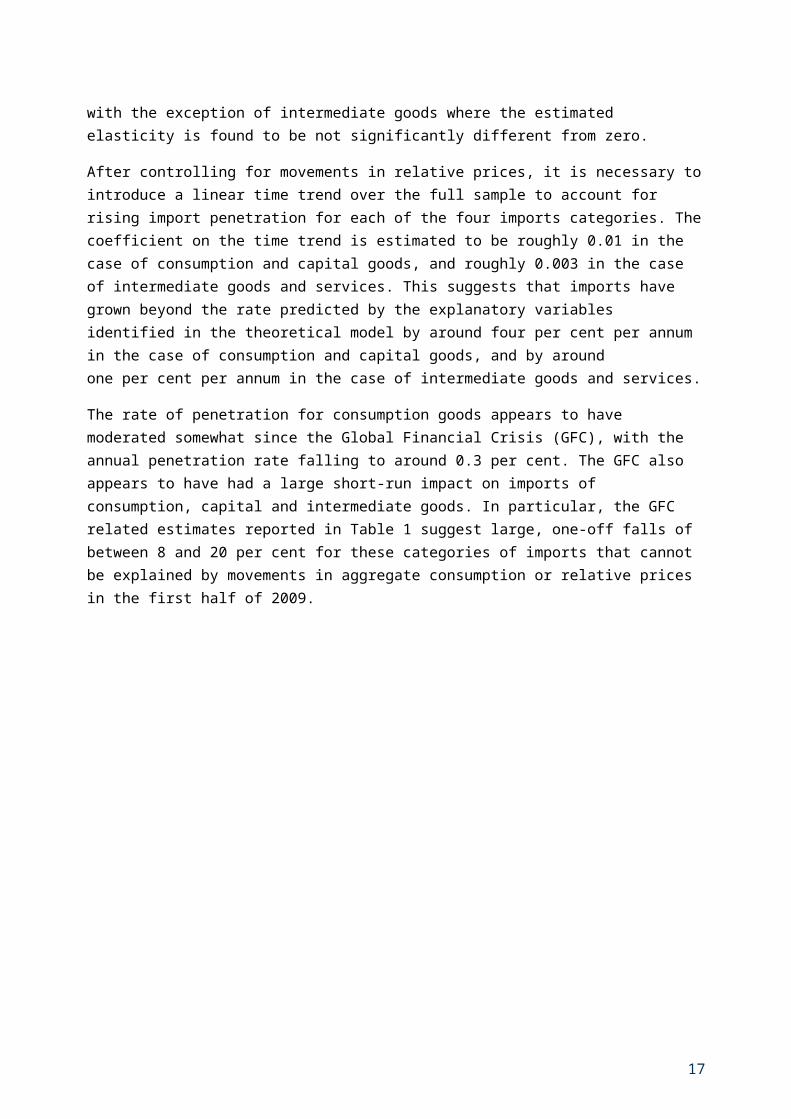
After controlling for movements in relative prices, it is necessary to introduce a linear time trend over the full sample to account for rising import penetration for each of the four imports categories. The coefficient on the time trend is estimated to be roughly 0.01 in the case of consumption and capital goods, and roughly 0.003 in the case of intermediate goods and services. This suggests that imports have grown beyond the rate predicted by the explanatory variables identified in the theoretical model by around four per cent per annum in the case of consumption and capital goods, and by around one per cent per annum in the case of intermediate goods and services.

The rate of penetration for consumption goods appears to have moderated somewhat since the Global Financial Crisis (GFC), with the annual penetration rate falling to around 0.3 per cent. The GFC also appears to have had a large short-run impact on imports of consumption, capital and intermediate

14

goods. In particular, the GFC related estimates reported in Table 1 suggest large, one-off falls of between 8 and 20 per cent for these categories of imports that cannot be explained by movements in aggregate consumption or relative prices in the first half of 2009.

Table 1: Estimation results – DemandConsumption Capital Intermediate Services

Long-run-0.6114 -0.4720 -0.6413 -1.2160(0.1557) (0.2820) (0.2209) (0.0962)-4.0400 -2.5366 -2.4304 -3.3783(0.2171) (0.4924) (0.1939) (0.0722)0.0096 0.0092 0.0027 0.0027

(0.0010) (0.0023) (0.0009) (0.0004)-0.0783(0.0422)

-0.0908(0.0186)-0.0910(0.0192)-0.0501(0.0204)

-0.0088 -0.0055(0.0024) (0.0020)

Short-run-0.2817 -0.3249 -0.1441 -0.3622(0.0585) (0.0612) (0.0471) (0.0577)1.3001 0.2835 0.8561 0.6283

(0.3762) (0.0875) (0.2917) (0.2183)-0.5449 -0.8471 -0.2651 -0.6800(0.1060) (0.1205) (0.0740) (0.0698)-0.0779 -0.1140 -0.1450(0.0303) (0.0512) (0.0276)

-0.2008(0.0516)

Summary statisticsR-squared 0.4721 0.5779 0.4220 0.7279Adjusted R-squared 0.4372 0.5458 0.3897 0.7046Durbin Watson 1.7801 1.8512 1.7245 1.9044ADF statistic -4.8701 -5.5338 -4.6083 -4.2890Sample 1985:3-2014:1 1985:3-2014:1 1985:3-2014:1 1985:3-2014:1

Note: Standard errors in parentheses. The aggregate consumption variable (that is, ct) used in the estimation of the four imports categories is as follows: consumption imports uses non-rental consumption; capital imports uses machinery and equipment investment; intermediate imports uses an aggregate of non-rental consumption and machinery and equipment investment; and services imports uses gross national expenditure.

The rate of penetration for services has also reversed since the GFC, with services now falling by around one per cent beyond the rate predicted by the explanatory variables in the model. How much of this is due to the GFC and how much is due to a general change in preferences is a topic of further research. The September 11 terrorist attacks, SARs virus, and GFC are also estimated to have had a permanent negative effect on the level of service imports in the order of 10, 10 and 5 per cent respectively.

Adjustment to the long-run via the error correcting term is estimated to be relatively fast for consumption goods, capital goods and services, with the coefficient on the error correcting term

15

suggesting it takes between 3 and 4 quarters to adjust back towards the long-run level of imports demand. Adjustment towards the long-run desired level of intermediate goods is relatively slow, and takes around 7 quarters.

The coefficient estimates reported in Table 1 indicate imports of consumption goods are highly sensitive to fluctuations in the aggregate consumption variable in the short-run, with imports of services and capital and intermediate goods less sensitive. A one per cent increase in aggregate consumption leads to a 1.3 per cent increase in imports of consumption goods, and a 0.6, 0.3 and 0.9 per cent increase in imports of services and capital and intermediate goods respectively. The short-run elasticity (or price effect) is lower than the long-run elasticity for consumption goods, intermediate goods and services. This suggests that these varieties of imports are less substitutable for domestic varieties in the short-run.

Chart 6: Long-run residuals – Demand

-.15

-.10

-.05

.00

.05

.10

.15

.20

.25

86 88 90 92 94 96 98 00 02 04 06 08 10 12 14

CONSUMPTION

-.3

-.2

-.1

.0

.1

.2

.3

.4

86 88 90 92 94 96 98 00 02 04 06 08 10 12 14

CAPITAL

-.16

-.12

-.08

-.04

.00

.04

.08

.12

.16

86 88 90 92 94 96 98 00 02 04 06 08 10 12 14

INTERMEDIATE

-.10

-.05

.00

.05

.10

.15

86 88 90 92 94 96 98 00 02 04 06 08 10 12 14

SERVICES


The long-run residuals of the four models are plotted in Chart 6. They are characterised by large cyclical fluctuations over the full sample. Applying the Augmented Dickey-Fuller (ADF) test to the long-run residuals for each of the categories of imports yields test statistics of between -4.3 and -5.6. This leads us to reject the null of a unit root (that is, reject the null of no cointegration) at conventional levels of significance.

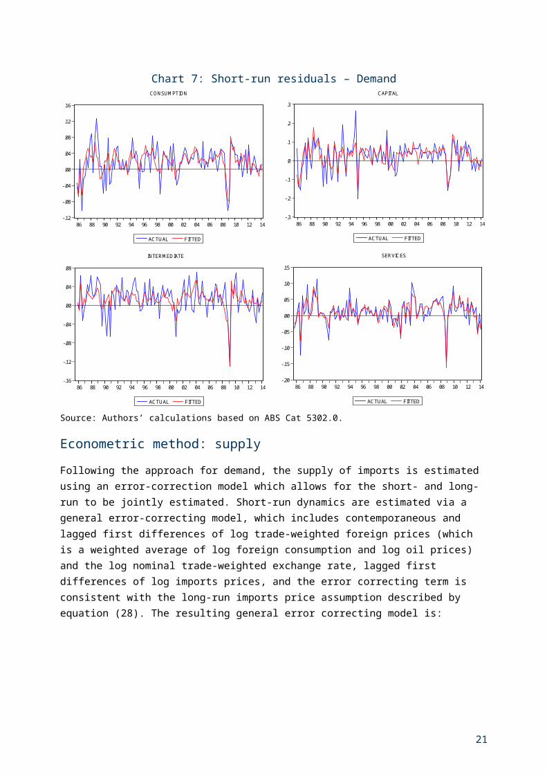
Finally, Chart 7 highlights the volatility of the quarterly growth rates of the four imports categories; the overall fit of the model; and the extent to which the exogenous shift terms capture the downturn caused by the GFC, September 11 terrorist attacks and SARs virus.

16

Chart 7: Short-run residuals – Demand

-.12

-.08

-.04

.00

.04

.08

.12

.16

86 88 90 92 94 96 98 00 02 04 06 08 10 12 14

ACTUAL FITTED

-.3

-.2

-.1

.0

.1

.2

.3

86 88 90 92 94 96 98 00 02 04 06 08 10 12 14

ACTUAL FITTED

-.16

-.12

-.08

-.04

.00

.04

.08

86 88 90 92 94 96 98 00 02 04 06 08 10 12 14

ACTUAL FITTED

-.20

-.15

-.10

-.05

.00

.05

.10

.15

86 88 90 92 94 96 98 00 02 04 06 08 10 12 14

ACTUAL FITTED

CONSUMPTION CAPITAL

INTERMEDIATE SERVICES


Econometric method: supply

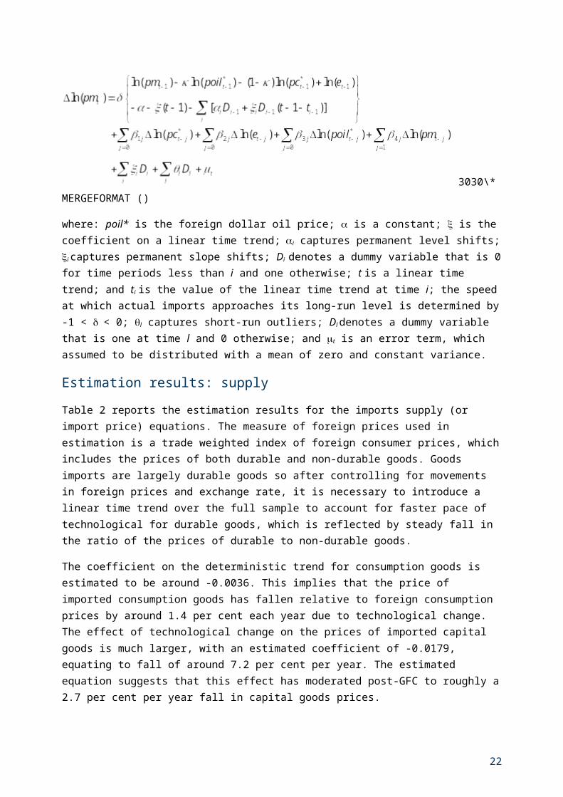
Following the approach for demand, the supply of imports is estimated using an error-correction model which allows for the short- and long-run to be jointly estimated. Short-run dynamics are estimated via a general error-correcting model, which includes contemporaneous and lagged first differences of log trade-weighted foreign prices (which is a weighted average of log foreign consumption and log oil prices) and the log nominal trade-weighted exchange rate, lagged first differences of log imports prices, and the error correcting term is consistent with the long-run imports price assumption described by equation (28). The resulting general error correcting model is:


17

where: poil* is the foreign dollar oil price; is a constant; is the coefficient on a linear time trend;i captures permanent level shifts; i captures permanent slope shifts; Di denotes a dummy variable that is 0 for time periods less than i and one otherwise; t is a linear time trend; and ti is the value of the linear time trend at time i; the speed at which actual imports approaches its long-run level is determined by -1 < < 0; l captures short-run outliers; Dl denotes a dummy variable that is one at time l and 0 otherwise; and t is an error term, which assumed to be distributed with a mean of zero and constant variance.

Estimation results: supply

Table 2 reports the estimation results for the imports supply (or import price) equations. The measure of foreign prices used in estimation is a trade weighted index of foreign consumer prices, which includes the prices of both durable and non-durable goods. Goods imports are largely durable goods so after controlling for movements in foreign prices and exchange rate, it is necessary to introduce a linear time trend over the full sample to account for faster pace of technological for durable goods, which is reflected by steady fall in the ratio of the prices of durable to non-durable goods.

The coefficient on the deterministic trend for consumption goods is estimated to be around -0.0036. This implies that the price of imported consumption goods has fallen relative to foreign consumption prices by around 1.4 per cent each year due to technological change. The effect of technological change on the prices of imported capital goods is much larger, with an estimated coefficient of -0.0179, equating to fall of around 7.2 per cent per year. The estimated equation suggests that this effect has moderated post-GFC to roughly a 2.7 per cent per year fall in capital goods prices.

Intermediate goods include imported petroleum products, so the foreign price term is augmented by the foreign price of oil. The estimated weight on oil prices is roughly 0.18, which is roughly equal to the average share of fuel and lubricants in intermediate goods imports over the sample period.

The coefficient estimates reported in Table 2 indicate that the price of capital and intermediate goods is very sensitive to fluctuations in foreign prices in the short-run. If foreign prices increase by one per cent, this is estimated to lead to a 2 per cent increase in the price of capital imports, and a 5.5 per cent increase in the price of intermediate imports. The supply of consumption goods and services are less sensitive to short-run movements in foreign prices, with both the foreign price and exchange rate coefficients less than one (in absolute terms). The coefficients on the short-run exchange rate term, suggests that all import prices will fall by less than one per cent in response to a nominal appreciation of one per cent.

Adjustment to the long-run desired price level ranges from around 1.5 quarters in the case of imports of capital goods, to 7 quarters in the case of imports of services. Coefficients on dummy variables suggest that the price of capital goods rose by around 5 per cent in 2008:4 and 11.5 per cent in 2009:1, over and above what can be explained by movements in foreign prices and the nominal exchange rate at the time of the GFC.

18

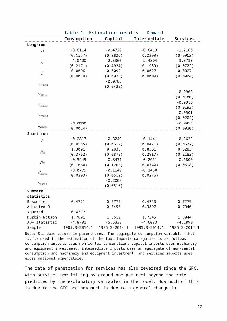
Table 2: Estimation results – SupplyConsumption Capital Intermediate Services

Long-run4.0947 6.9760 1.7971 3.4604

(0.0595) (0.0500) (0.1321) (0.0206)-0.0036 -0.0179(0.0003) (0.0003)

0.1785(0.0180)0.0524

(0.0206)-0.0076(0.0022)

-0.0287(0.0128)

0.0112 -0.0042(0.0010) (0.0011)

Short-run-0.1987 -0.6910 -0.3651 -0.1420(0.0518) (0.0993) (0.0760) (0.0475)0.8183 1.9814 5.4564 0.7903

(0.4273) (0.9642) (0.8253) (0.3955)-0.6307 -0.5681 -0.8461 -0.7758(0.0336) (0.0903) (0.0687) (0.0347)

0.0906(0.0245)

0.0513(0.0218)0.1158 -0.0442

(0.0368) (0.0107)Summary statisticsR-squared 0.8437 0.7422 0.7444 0.9107Adjusted R-squared 0.8348 0.7152 0.7177 0.9028Durbin Watson 2.0929 2.0951 2.0353 1.9047ADF statistic -3.3153 -3.2520 -3.3562 -2.8576Sample 1995:3-2014:1 1995:3-2014:1 1995:3-2014:1 1995:3-2014:1

Note: Standard errors in parentheses

Chart 8 plots the long-run residuals for the four import price categories. Again, they are characterised by large and persistent cyclical fluctuations throughout the sample. Applying an ADF test to these residuals yields low test statistics, which suggests that a difference equation may be a more appropriate specification to model the supply of imports. These results suggest that while there is reasonably strong pass-through of foreign prices and exchange rate movements to imports prices in the short-run, there is weak evidence in favour of the law of one price in the long-run.

19

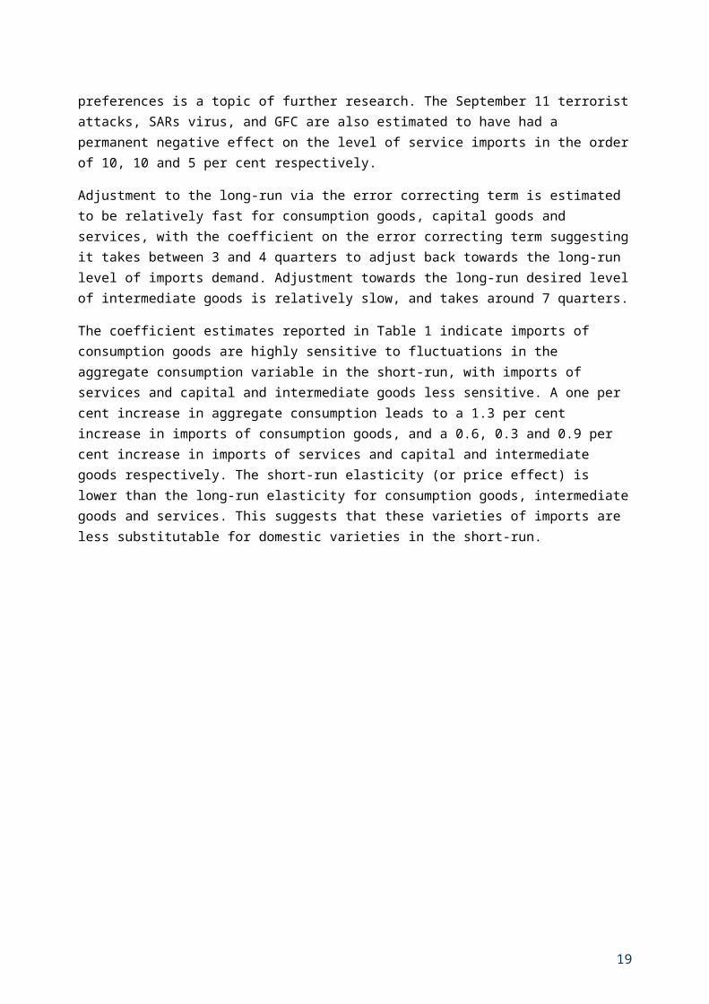
Chart 8: Long-run residuals – Supply

-.12

-.08

-.04

.00

.04

.08

1996 1998 2000 2002 2004 2006 2008 2010 2012 2014

CONSUMPTION

-.100

-.075

-.050

-.025

.000

.025

.050

.075

.100

1996 1998 2000 2002 2004 2006 2008 2010 2012 2014

CAPITAL

-.08

-.04

.00

.04

.08

.12

1996 1998 2000 2002 2004 2006 2008 2010 2012 2014

INTERMEDIATE

-.08

-.06

-.04

-.02

.00

.02

.04

.06

1996 1998 2000 2002 2004 2006 2008 2010 2012 2014

SERVICES


Dwyer and Lam (1994) estimate a similar model, using the import price of consumption goods as their dependent variable. They present considerably stronger evidence in favour of cointegration. Aside from the fact that they estimate their equations over a different time period, one possible reason for this result is their use of an index of world export prices for consumption goods as the foreign price variable. In light of their analysis, we would prefer to use a foreign price variable that was a closer match to the respective import bundles for consumption, capital, intermediate and services. However, the models presented here are used to forecast imports volumes and prices, so it is critical that the foreign price variable be forecastable. Treasury’s forecast system recognises that forecasts of foreign country prices for exports (and all other goods) are ultimately based on more readily available forecasts of foreign CPIs. Therefore to ensure the best possible forecasting model we model import prices directly using a foreign CPI index, rather than model import prices as a function of a foreign export price index and then forecast the export price index via secondary model that relates foreign export prices to foreign CPIs.

Chart 9 shows that despite their very large amplitudes, the short-run fluctuations in the prices of imports are largely explained by the fundamental drivers identified in the theoretical model.

20

Chart 9: Short-run residuals – Supply

-.08

-.04

.00

.04

.08

.12

.16

1996 1998 2000 2002 2004 2006 2008 2010 2012 2014

ACTUAL FITTED

-.15

-.10

-.05

.00

.05

.10

.15

.20

.25

1996 1998 2000 2002 2004 2006 2008 2010 2012 2014

ACTUAL FITTED

-.12

-.08

-.04

.00

.04

.08

.12

1996 1998 2000 2002 2004 2006 2008 2010 2012 2014

ACTUAL FITTED

-.08

-.04

.00

.04

.08

.12

.16

1996 1998 2000 2002 2004 2006 2008 2010 2012 2014

ACTUAL FITTED

CONSUMPTION CAPITAL

INTERMEDIATE SERVICES


5. CONCLUSION

This paper models both the supply and demand of Australian imports. It builds on earlier demand modelling by Wilkinson (1992); Jilek, Johnson and Taplin (1993); and Dwyer and Kent (1993) by deriving long-run import demand relationships from first principles. These long-run relationships are augmented by cyclical explanatory variables to form error correction models, which are estimated using quarterly data for disaggregated imports categories (consumption goods, capital goods, intermediate goods and services) from 1985:3 to 2014:1. Our estimates are consistent with previous Australian studies in finding relatively low substitutability between imported and domestically produced varieties of goods. The main implication is that income effects will dominate, so that a rise in import prices will lead to a fall in both the demand of the imported good and the domestically produced import substitute. Service imports are found to be gross substitutes, with a rise in the price of imports leading to greater demand for domestically produced services.

We also model the supply of imports, assuming that households/firms are price takers in the long-run (that is, the import prices equal to the exchange rate adjusted foreign cost). Our estimates suggest while there is reasonably strong pass-through of foreign prices and exchange rate movements to imports prices in the short-run, there is weak evidence in favour of the law of one price in the long-run.

21

REFERENCES

Australian Bureau of Statistics (2011) Balance of Payments and International Investment Position, Australia: Concepts, Sources and Methods, ABS. Cat. No. 5331.0

Australian Bureau of Statistics (2012) Feature article: mining investment in ABS publications, Private New Capital Expenditure and Expected Expenditure, ABS Cat. No. 5625.0, March 2012.

Becker, C. and M. Davies (2002) Developments in the trade-weighted index, Reserve Bank of Australia Bulletin, October.

Caton, C.N. and H.N. Johnston (1975) An econometric model of the Australian economy, Australian Bureau of Statistics.

Chung, E., M. Kohler, and C. Lewis (2011) The exchange rate and consumer prices, Reserve Bank of Australia Bulletin, September Quarter, pages 9-16.

Dixit, A.K. and J.E. Stiglitz (1977) Monopolistic competition and optimum product diversity, American Economic Review, Vol. 67, No. 3, pages 297-308.

Dwyer, J. and C. Kent (1993) A re-examination of the determinants of Australia’s imports, Reserve Bank of Australia Discussion Paper, No. 9312.

Dwyer, J. and R. Lam (1994) Explaining import price inflation: a recent history of second stage pass-through, Reserve Bank of Australia Discussion Paper, No. 9407.

Jilek, P., A. Johnson, and B. Taplin (1993) Exports, imports and the trade balance, Treasury Macroeconomic (TRYM) Model Papers, Australian Treasury.

Kouparitsas, M.A. and L. Luo (2014) Modelling Australia’s exports of goods and services, Treasury Working Paper, forthcoming.

Wilkinson, J. (1992) Explaining Australia’s imports: 1974-1989, Economic Record, No. 68(201), pages 151-164.

22


APPENDIX A: DATA SOURCES

Australian Bureau of Statistics, Balance of Payments and International Investment Position, Australia, ABS Cat. No. 5302.0, December 2012: imports volumes and prices; and trade-weighted non-exchange rate index.

Australian Bureau of Statistics, Australian National Accounts: National Income and Product, Australia, ABS. Cat. No. 5206.0., December 2012: gross national expenditure volumes and prices; aggregate household consumption volumes and prices; rental services volumes and prices; and gross fixed capital expenditure: machinery and equipment volumes and prices.

Various national statistical agencies: foreign, local-currency denominated, consumption prices.

23


Modelling Australia's imports of goods and services€¦ · Web viewWe build on earlier demand...

Documents

Transcript of Modelling Australia's imports of goods and services€¦ · Web viewWe build on earlier demand...