TOWARDS IMPROVED QUANTITATIVE CHARACTERIZATION OFCORRODING SURFACES USING FRACTAL MODELS

IK R TRETHEWEY and 2p R ROBERGEIRoyal Naval Engineering CollegeManadonPlymouth PL5 3AQ, UK

lRoyal Military CollegeKingstonOntario, Canada, K7K 5LO

ABSTRACT. Techniques recently shown to be effective in the analysis of electrochemical noisehave been used to investigate the quantitative information to be gained from topographicalprofiles of corroding surfaces. Representation of both uncorroded and corroded surfaces byfractals has been examined and a comparison of traditional coastline plots with other methodsofanalysis carried out. A new method known as the Stochastic Pattern Detector is shown to bea particularly sensitive tool for highlighting high resolution changes to surface profile duringcorrosion of aluminium 2024. Correlation of conventional mechanical surface profilemeasurements and rescaled range analysis has been achieved.

1. Introduction

Quantification of localized corrosion remains a difficult engineering problem inmany industries [1] and a variety of strategies are being employed in our laboratoriesto improve this situation [2-5J. In aluminium alloys, stress raisers caused by pittingand grain boundary corrosion, for example, continue to give rise to potentiallycatastrophic corrosion failures, despite the introduction of supposedly superiormaterials. The benefits to be gained from introduction of newer alloys, such as thealuminium lithium series and the latest range of metal matrix composites based onaluminium alloys, must be weighed against the continued likelihood of theseproblems. Uncertainty in life prediction is a natural consequence of localizedcorrosion and until new methods are provided for the quantification of the highcorrosion rates found in localized attack, problems are likely to continue. The recentdevelopment of methods for analysis of non-linear dynamic systems promises tomake a great impact in corrosion engineering.Science and engineering were recently given a considerable boost by development

of the new fields of chaos, by such people as Lorenz [6] and Feigenbaum [7], andfractals by Mandelbrot [8]. Both were soon realized to have immense application tothe study of natural phenomena in a wide variety of disciplines. Chaos, for example,has recently been found in a number of instances of corrosion and varioustechniques for its analysis have been applied to metallic dissolution [9, 10].

443

K. R. Trethewey and P. R. Roberge (eds.), Modelling Aqueous Corrosion, 443-463.© 1994 British Crown.

444

'Fractal' is a term which describes complex patterns, shapes, curves or functionswhich can be expressed by

bulk '" sizedimeMOtI (1)

in which dimension is almost always a non-integer. The proposition by Mandelbrotthat dimension, rather than being strictly Euclidean (and integral) could also befractional (hence the term, 'fractal') has proved to be remarkably successful, with theresult that considerable progress has recently been made in a number of areas ofscience. Success has been demonstrated in the application of fractals tomeasurements of coastlines (11], with logical extensions to pit profiles [1, 12]. Sincethen, numerous workers have extended the theories of fractal geometry to relatedsubjects such as flow through porous media [13] theories of multilayer adsorptionof gases [14] and bimolecular chemical reactions [15]. Fractals have also beenapplied to electrochemical impedance in corrosion [16-19].

It is natural to suppose that the new mathematics of fractal geometry might leadto advances in areas of corrosion science which have so far proved to be resistantto quantitative description, in particular localized attack and pitting. Description ofcorroding surfaces with fractals has already been reported by us [20, 21]. This paperbuilds on the initial foundations laid in the earlier studies and explores the value ofsome new analytical techniques. A pivotal part of this approach is the correlationbetween the kinds of traces obtained from surface profile with time series analyses.In the latter, well-established mathematical functions are used [22, 23], spectraldensity plots can be computed using fast Fourier transforms (FFf) or otheralgorithms such as the Maximum Entropy Method (MEM) [24, 25].This paper focuses on two new techniques in corrosion: the Stochastic Pattern

Detector (SPD) technique [26] and Rescaled Range Analyses (R/S) [27]. The SPDtechnique is shown to be especially advantageous for delineation of localizedfeatures at a given magnification, whilst the R/S technique can provide a moreversatile method of determination of fractal dimension than the frequently usedcoastline plot.

2. Theory

2.1 COASTLINE ANALYSIS- TIffi RICHARDSON PLOT

The representation of a 'natural' surface such as a corroding metaVelectrolyteinterface by means of a fractal is best introduced by means of the theory ofmeasurement of coastline length [8] in which a measurement is dependent upon thelength of the ruler used. As the scale of measurement becomes smaHer, so thelength of the interface between land and sea, measured at sea level, increases. Thisis expressed by the empirical equation

445

(2)

in which L(e) is the coastline measured by a ruler of length e, F is a constant andD is the fractal dimension. When plotted as

logL(e) = logF + (l-D)log(e) (3)

a straight line is obtajned of slope (I-D). In the case of a true fractal, theimplication is that the smaller the scale (greater the magnification) the greater is theamount of detail to be measured. Thus although the ruler becomes smaller, thedetail of the surface is by implication always smaller than the length of the ruler.Hence it is not meaningful to discuss the length of the coastline of a truly naturalsurface on a geographical scale since its details will be ultimately defined by atoms.One commonly used technique in applications of coastline analysis techniques

is described by Saupe [28]. Costa and Vilarrasa [12] use such a method in theirinvestigation of pitting corrosion of stainless steel. Joosten and co-workers have alsoadopted coastline techniques in their estimations of CO2 pitting attack in pipelinematerials. Both groups examined pitting intensity by digitising maps of the pittingand both techniques involved time-consuming material grinding techniques to revealpitting structure for analysis. Costa and Vilarrasa worked with surface pits in two(Euclidean) dimensions and reported changes in the pit geometry at various depthsby removal of successive surface layers, thus extending their analysis into threedimensions. Their method involves covering a map of pits by a grid of squares ofside e and the length of the coastline is obtained by taking the number of squarescovering the coastline and multiplying by 2e. By carrying out a sequence ofiterations for different e, a plot of log L versus log e (known as a Richardson plot)is drawn. Assuming, as in this case, that a linear relationship is observed, the slopeand hence D may be found. The significance of D is that as the surface becomes'rougher', and thus more 'space-filling', D is expected to increase between theEuclidean value for a straight line of 1 and the Euclidean 2 for a plane. (Whenconsidering areas occupied by islands, the value of D increases between 2 and 3.)Costa and Vilarrasa found that as successive layers were removed from the surface,the value of D increased slightly, suggesting that the pits were becoming more'irregular' in shape with depth into the material. They also reported two slopes fordifferent parts of the coastline curve. This was ascribed to a difference between astructural and a textural fractal. Thus the coarse structure of the pit boundaries wasreported as having fractal dimension D = 1.45, whilst corroded, fine-texturedsurfaces showed D = 1.17.

2.2. RESCALED RANGE (RlS) ANALYSIS

Originally proposed by Hurst [29], the rescaled range analysis technique has been

446

used by Mandelbrot and co-workers for determination of the fractal characteristicsof time series [30, 311. Known as the R/S technique, R or R(t,s) stands for thesequential range of the data points increments for a given lag (s) and time (t), andS or Set,s) for the square root of the sample sequential variance. A detaileddescription of this analysis can be found in the work by Fan [27]. Hurst [29] andlater Mandelbrot and Wallis [31] have proposed that the ratio R(t,s)/S(t,s), alsocalled the rescaled range, is itself a random function with a scaling propertydescribed by

(4)

where the scaling behaviour of a signal is characterized by the Hurst exponent (H)which can vary between 0<H< 1. It has additionally been shown [32] that the localfractal dimension, 0, of a fractional Brownian motion (fBm) time series is relatedto H by

D=2-H,O<H<1 (5)

This makes it possible to characterise the fractal dimension of a given time seriesby calculating the slope of a R/S plot.

2.3. SPD TECHNIQUE

The Stochastic Pattern Detector (SPD) Technique was developed by one of us [26]for determining the level of stochasticity (as opposed to determinism) inelectrochemical noise data. Since electrochemical noise and surface profiles are bothtime series, the technique has here been applied to analysis of corroding surfaceprofiles. The technique consists of transforming voltage or signal fluctuations intoindividual peaks as basic events [33]. The rise times of the basic events, dV/dt, arethen computed. Next, the probability distribution of the basic events is comparedwith an ideal Poisson probability distribution of stochastic point processes. Ameasure of the goodness-of-fit is evaluated by comparing the ideal exponentialdistribution to the experimental distributions observed and corresponding toindividual At where

(6)

and subsequently averaged to give Amean• The goodness-of-fit is given by anexpression of the difference between this average and the ideal value, A, thus,

3. Experimental

3.1. CORROSION

AGoodness-of-fit(%);(l-ll-~ 1).100%

A

447

(7)

A sample of rolled aluminium 2024 sheet, nominal composition Si: 0.5%, Fe: 0.5%,Cu: 4.3%, Mn: 0.6%, Mg: 1.5%, Zn: 0.25%, of dimensions 100 x 40 x 4 mm wasground to a 600 grit finish and stood in a 250 ml beaker such that it was immersedin aerated 3% NaCI solution to a level about 30 mm from the top of the specimen.The effect of aeration created a 'splash zone' over the surface of the specimen whichwas not immersed. During the course of exposure, a portion of the immersed regionin the centre of the upward-facing surface became covered in gas bubbles andsuffered a higher level of attack than the rest of the immersed surface. After 24hours the plate was removed from the solution. No cleaning procedures were usedand it is appreciated that corrosion product would have been present on all surfacesduring measurement. Figure 1 shows in diagrammatic form the specimen and areasfrom which the surface profiles were measured.

3.2. PROFILE MEASUREMENTS

Surface profile measurements made in all of the various planes, i.e. LT, TL, LS, SL,ST and TS. Measurements were made by means of a Rank Taylor Hobson FormTalysurf with a 0.2 JLm diamond tip probe. The instrument creates a line scan of areal surface by pulling the probe across a pre-defined part of the surface at 1 mmS·I. All traces were of length 8 mm, generating 32K points with a sampling rate of0.25 JLm, except in the case of the ST and ST directions which, because of the platethickness, were limited to 2 mm traces.Let us define the co-ordinate axes in the plane of the surface as x and y. Vertical

deviations (in the z-axis) are measured and the data is digitised and stored in theform of an x-z map. The set of x-z co-ordinates form the familiar description of asurface. It is important to realise that since the equipment is recording az-displacement of the probe with time, the usual x-z geometrical description isactually a time series. To facilitate the visualisation process, the display is distortedbecause of the use of different scales to plot the x and z information. Thus, forexample, x is usually plotted in mm, whilst z is plotted in JLm. The problem ofhuman visualisation exists because a real surface plotted with two such differentscales on the x- and z-axes does not 'look' real. However, when both axes are plottedon the same scale, the surface can be seen to be much 'smoother' than at firstthought; indeed, it is very difficult for the human eye to distinguish the featureswhich are under scrutiny.

448

___bo_tt_o_m__~ surface 85(S1), 86(TS)

surface 71 (LS) , 77(SL)

surfaces 125 (L1) I 129(TL)

heavy pittingto generalcorrosion:

'scar'

+TL

LT

pitted- dark colour

l.--_--_--_to---'--p_-_--_-_--=+- surface 112(S1), 117(TS)

surfaces 106 (L1), 109 (TL)~-+- surfaces 92 (L1), 94 (TL)

surface 96(LS), 102(SL)

sprayzone pitted- light colour

t+1S

S1

t light pitting

immersed

LS

side

Figure 1 - Schematic diagram of co"oded aluminium plate showing locations of different corrodedzones and identifying the surface profiles listed in Table 1.

3.3. SOFfWARE ANALYSIS

The manufacturer's software for the Talysurf instrument was used for the analysis,it being capable of generating over twenty surface profile parameters. In this studythree parameters, Ra, Rt and S were examined. Ra, the roughness average isdescribed as the average deviation from a mean line, whilst Rt is the distance fromthe deepest pit to the highest peak of the profile, an index which was taken as anengineering 'worst case' parameter for pitting severity. Ra and Rt are thus bothz-direction parameters. S, on the other hand, is the mean distance betweenintercepts of the x-axis mean line. The software carries out analysis of raw data ina sophisticated but standard way, allowing for filtering of values to remove unwanted

449

0500 1000 1500 2000 2500 3000 3500 4000

-500

-1000

-1500

-2000

5000

-500-1000-1500-2000-2500-3000-3500-4000-4500-5000

4000

2000

0

-2000

-4000

-6000

-8000-10000

-12000

30000

25000

20000

15000

10000

5000

500 1000 1500 2000 2500 3000 3500 4000

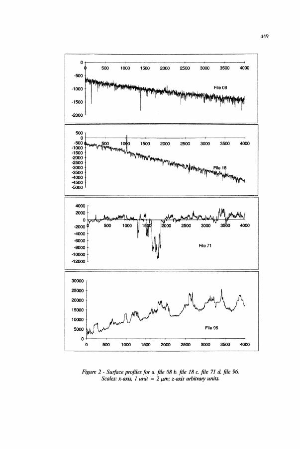
Figure 2 - Surface profiles for a. file 08 b. file 18 c. file 71 d file 96.Scales: x-axis, 1 unit =2 1J11I; z-axis arbitrary units.

450

form and waviness from the profiles. It is impossible to eliminate filtering effectscaused by the probe tip which, depending on surface profile, is better able tomeasure high points on the profile than low points. Inevitably, any profile obtainedby mechanical means will carry some character resulting from the measurementmechanism. We are currently evaluating the use of an SEM beam as a more efficientprobe for correlation with mechanically-derived profiles.R/S, SPD and Richardson coastline analyses were all carried out using

locally-produced software. In the R/S analyses, a 'scanning' technique was adoptedin which a typical trace of 32K points was subdivided into segments, each of length,IK and stepping in increments of 200 for each segment. Segments were analysed andgraphs of 10g(R/S) versus log (s) plotted; slopes (H) of each graph were determined.Each step of 200 along the profile generated a value of fractal dimension, D (=2-H)and the mean and standard deviation were determined for each profile (Table I).

4. Results

The corrosion found on the plate varied considerably from area to area. The regionof the plate beneath the gas bubbles was found to be particularly badly corroded, theconcentration of pits being so high that the area had become one of almost generalcorrosion. Across the remainder of the immersed upward-facing surface, the pittingwas scattered. The 'splash zone' of the surface above the electrolyte was quite badlypitted, worse so than the immersed region. On the sides, pits were clearly evidentand of a geometry and orientation which conformed to the expected grain structureof the rolled material.Table 1 combines values of surface profile parameters obtained by the Talysurf

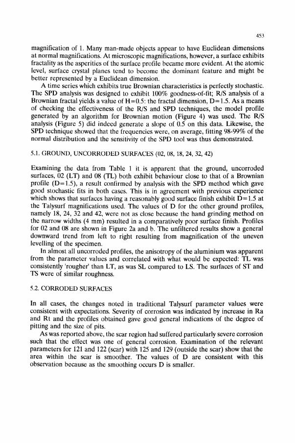
with values of fractal dimension, D, and associated standard deviation for all theareas of the surface investigated. Figure 2(a-d) shows surface profiles 08, 18, 71 and96. Figure 2a is of the original (uncorroded, ground) LT surface used as a control.Figs. 2b-d are all taken in the LS direction with Figure 2b, a similar uncorrodedtrace, Figure 2c a region of corroded, immersed-zone metal showing a lowpopulation of large pits, and Figure 2d a region of the spray zone in whichparticularly well developed, rounded pits were obtained. Figure 3 shows the graphof log (L) vs log (e) (Richardson coastline analysis) for the two profiles, 08 and 96.For control purposes, data was generated which would indicate the effectiveness orotherwise of the analysis techniques selected. Figure 4 is a profile of lK pointsgenerated from an algorithm for Brownian motion with D= 1.5 [34] and Figure 5 theR/S analysis of the profile in Figure 4.

5. Discussion

The promise of fractals in their applications to quantitative desrciptions of localized

45\

TABLE 1Measured and calculated parameter values for profiles taken from the regions of

the specimen shown in Figure 1.

File D StDv Ra Rt S

LT 2 1.407 0.060 0.108 2.400 9.770

LT 92 1.244 0.099 1.470 18.355 17.605

LT 121 1.312 0.105 0.447 6.843 10.416

LT 125 1.418 0.062 0.698 14.414 18.704

LT 106 1.282 0.091 0.937 13.847 18.386

11.. 8 1.477 0.057 0.155 3.496 7.071

11.. 94 1.296 0.107 1.239 21.589 15.905

11.. 109 1.259 0.117 1.295 21.361 16.178

TL 122 1.407 0.088 0.512 10.789 10.220

TL 129 1.417 0.097 0.708 11.145 11.537

LS 18 1.281 0.062 0.279 4.087 12.293

LS 96 1.215 0.102 1.363 15.791 17.936

LS 71 1.316 0.139 0.645 11.104 14.003

SL 24 1.377 0.088 0.282 3.167 7.727

SL 77 1.280 0.081 1.023 18.588 12.951

SL 102 1.226 0.103 1.824 15.666 15.209

TS 42 1.399 0.060 0.316 4.370 9.561

TS 117 1.394 0.083 0.901 15.233 12.796

TS 86 1.373 0.127 1.076 14.669 13.416

ST 32 1.424 0.061 0.328 3.970 9.462

ST 85 1.327 0.128 0.935 20.607 13.865

ST 112 1.369 0.114 0.635 13.883 13.078

452

corrosion is considerable. At first sight, the description of a system at various stagesof corrosion by a fractal dimension might seem straightforward, but there are manyproblems to be overcome. Real surfaces contain a wide range of different features,often distributed non-uniformly over a surface. The texture of the surface within agrain would be expected to be considerably different from that at the grain boundary[35] or of a pitted surface. The geometry of pits is itself a very complex field of studyand has contributed much to the difficulties of quantification of corrosion damage.

Coasdlne analysis 01 curves 08 and 96

5.8 ~

·2

~~

·1

5.6 T

I

I5.2 ..,

5 +I

.. t46 I4.4 ,

o 1

logINI•• length)

2

Figure 3 - Coastline analysis (Richardson plot) ofprofiles 08 and 96.

The concept of self-similarity described by Mandelbrot is important. This meansthat fractal surfaces look similar at whatever magnification they are viewed. Twoproblems at once arise when dealing with real surfaces. First, whilst it may bepossible to construct computer models able to describe real surfaces to this degreeof detail, most laboratory measurements deal with surfaces modelled using digitisedmapping. Inevitably, because a surface (whether real or modelled) is represented byan array of co-ordinates, this reduces the fractal character of the surface recordwhich, in turn, imparts curvature to the log-log plot of eqn (3). A further practicalconsequence of working with digitised data which causes difficulty is that when the'ruler length' exceeds a certain value, the resultant coastline length becomesmeaningless.The second difficulty is that real surfaces do not necessarily exhibit the same

degree of fractality at all magnifications. For example, a specimen with a ground andpolished surface might appear to have a Euclidean dimension (i.e. 1) at a

453

magnification of 1. Many man-made objects appear to have Euclidean dimensionsat normal magnifications. At microscopic magnifications, however, a surface exhibitsfractality as the asperities of the surface profile became more evident. At the atomiclevel, surface crystal planes tend to become the dominant feature and might bebetter represented by a Euclidean dimension.A time series which exhibits true Brownian characteristics is perfectly stochastic.

The SPO analysis was designed to exhibit 100% goodness-of-fit; R/S analysis of aBrownian fractal yields a value of H=O.5: the fractal dimension, 0= 1.5. As a meansof checking the effectiveness of the R/S and SPO techniques, the model profilegenerated by an algorithm for Brownian motion (Figure 4) was used. The R/Sanalysis (Figure 5) did indeed generate a slope of 0.5 on this data. Likewise, theSPO technique showed that the frequencies were, on average, fitting 98-99% of thenormal distribution and the sensitivity of the SPO tool was thus demonstrated.

5.1. GROUND, UNCORRODED SURFACES (02, 08, 18, 24, 32, 42)

Examining the data from Table 1 it is apparent that the ground, uncorrodedsurfaces, 02 (LT) and 08 (TL) both exhibit behaviour close to that of a Brownianprofile (0= 1.5), a result confirmed by analysis with the SPO method which gavegood stochastic fits in both cases. This is in agreement with previous experiencewhich shows that surfaces having a reasonably good surface finish exhibit 0=1.5 atthe Talysurf magnifications used. The values of 0 for the other ground profiles,namely 18, 24, 32 and 42, were not as close because the hand grinding method onthe narrow widths (4 mm) resulted in a comparatively poor surface finish. Profilesfor 02 and 08 are shown in Figure 2a and b. The unfiltered results show a generaldownward trend from left to right resulting from magnification of the unevenlevelling of the specimen.

In almost all uncorroded profiles, the anisotropy of the aluminium was apparentfrom the parameter values and correlated with what would be expected: TL wasconsistently 'rougher' than LT, as was SL compared to LS. The surfaces of ST andTS were of similar roughness.

5.2. CORRODED SURFACES

In all cases, the changes noted in traditional Talysurf parameter values wereconsistent with expectations. Severity of corrosion was indicated by increase in Raand Rt and the profiles obtained gave good general indications of the degree ofpitting and the size of pits.As was reported above, the scar region had suffered particularly severe corrosion

such that the effect was one of general corrosion. Examination of the relevantparameters for 121 and 122 (scar) with 125 and 129 (outside the scar) show that thearea within the scar is smoother. The values of 0 are consistent with thisobservation because as the smoothing occurs 0 is smaller.

Distance (arbnrary units)

454

4000

2000

f~ -4000

i-.: I~ ·6000 ti II ·8000 Tis ·10000 t-12000 +

I-14000 t.16000 1

100 200 300 400 500 600 700 800 900 1000

Figure 4 - Brownian model profile generated by an algorithm [28j.

. .• •• •

•••

••

1.4 1.6 1.8

log (1l1li) (wbltraty ...Its)

2 2.2 2.4

Figure 5 - RlS analysis ofprofile in Figure 4. Slope of line is 0.499 on a data sample of 2048 points.

455

Perhaps surprisingly, the areas with the biggest reduction in D from 1.5 arethose with the greatest effect of pitting, i.e. traces 92, 94 and 96, all of whichoccurred in the spray zone above the electrolyte. This is explained by the relativelylarge macropits (Figure 2d) contributing a semi-circular nature to the fractal model,at the magnification appropriate to that measurement. Fine strucutre or pit initiationsites would be expected to have a completely different effect at a much greatermagnification.

5.3. CORRELATION OF TALYSURF ROUGHNESS AND HURST EXPONENT, H.

The analysis of the profiles using the R/S analysis provides further fractalinformation. Clearly, there is an approximate tenfold increase in Ra and Rt betweenthe polished (02 and 08) and the heavily corroded (94, 96 and 109) profiles. Ratherless increase is observed for the profiles 121, 122, 125 and 129. The behaviour of theHurst exponent, H, closely parallels that of Ra and Rt, Figure 6.

5.4. ANALYSIS OF THE RICHARDSON COASTLINE PLOT.

The Richardson coastline analysis was carried out on the two profiles, 08 and 96.Profile 08, shown in Figure 2a, was used because of its Brownian stochasticcharacter, whilst profile 96, shown in Figure 2d, was selected because it was aparticularly good example of high density spray zone pitting. The coastline plot isshown in Figure 3. The average total deviations from peak to valley of profile 08 isrepresented by twice the roughness average of the specimen, 0.155 j.£m, or 310 in thescale units of the z-axis of Figure 2a. Experience with coastline plots shows thatwhen the ruler length exceeds this value, the algorithm fails to give linearity. Thuson curve 08 of Figure 3, linearity plainly breaks down at ruler lengths greater thanlog (310), i.e. 2.5. At short ruler lengths, linearity also ceases because the data isessentially digitised and very short ruler lengths approach the precise length of thedigitised data, 2.5 x lOS.!n the region of log (E) from 1.7 to 2.5, good linearity isobtained with a slope of -0.61, and fractal dimension 0 = 1.61.In Figure 2d, the profile 96 shows at least two kinds of feature. Coarse pitting

structure is clearly visible with about six uniformly shaped hemispherical pits ofapproximate radius 37.5 /-Lm (150 x-scale units; 4 units = 1 /-Lm). Fine texture withinthe pits and other areas is also visible. Again, the average total deviations from peakto valley are approximately 5000 z-units which, on the coastline plot, Figure 3,correlates with the linearity breakdown at about log (E) = 3.7. Simple inspection ofthe scales shows that the fine texture of curve 96 is still coarser than the structureof curve 08. Thus, there is some instability in the linearity of the line at about log(E) = 2.8 as the ruler length becomes too long for good correlation with the finetexture, but is still adequate for resolving the coarse pitted structure. Indeed, thereis even evidence of a third kind of texture, intermediate between the fine texture andthe coarse pits, shown by the deviation in linearity at log (E) = 3.25; this is also to

456

be seen by inspection of the profile and may result from the original rollingdirectionality of the sheet material: further work is being carried out to examine thistheory. Taking the coarse pitted structure as being characterised by linearity from2.8 to 3.7, the slope is -0.52, D = 1.52. The slope of the fine textured part of theprofile is about -0.30, D= 1.30.

2.500 -

2.000

Tl

~Ra

---H

--+-- AVIO

LS SL TS ST

0.000 -'-----r--+----+----+--_+~______1~+---.---~___+__+_____t_~______1-+___+__+__+__;___+__+__+__i___l

proftl..

Figure 6 - Correlation of surface roughness parameter values with calculated Hurst exponents, H, forthe profiles in Table 1.

The overaJl effect of the corrosion process has been to increase the coastlinelength from 2.5 x lOS scale units for curve 08 to 5.0 x lOS scale units for curve 96, anincrease in length of 2.0. It is well worth pointing out at this stage how, if this regionof the specimen were totally immersed, this would have resulted in an approximatefourfold increase in the surface area of aluminium exposed to electrolyte and howdramatically, calculations of current density are affected. A further speculative pointis that with an atomic radius for aluminium of 142 pm, and an x-axis scale unitwhich equals 0.25 ",m, the limit of 'atomic resolution on the coastline plot using thescale adopted occurs at about -3.25. The difference in profile length, as evidencedby the separation of the two horizontal portions of the curves 08 and 96 isnevertheless limited by digitized data obtained from a diamond probe of limitinggeometry. However, it is possible that extrapolation of the corroded and polishedlines to -3.25 might yield a value of the actual increase in surface area exposed tothe electrolyte and hence to improved corrosion rate measurements. Thesearguments illustrate particularly well how the development of fractal models ofcorrosion may point the way to improved quantitative models of localised corrosion.

457

The use of Richardson coastline plots is clearly capable of identifying large scalefeatures consistent with comparatively large ruler lengths and seems to possesscharacteristics of different surface texture. As has been shown, the limitationsimposed by the mechanical measurement tool and consequent digitising of datamean that features consistent with particularly fine structure may not be observed.This might be overcome by the use of laser or SEM beam techniques. Subsequentsections will show that it is the digitising effect on the Richardson plot rather thanthe mechanical tool (Le. the Talysurf probe tip) that causes these limitations. Othertopographical information is indeed present in the data.

5.5. SPD ANALYSIS

In order to provide information about corrosion features at very high resolutionwhich could not be observed by the Richardson plot, analysis using the SPDtechnique was shown to be particularly effective. To create the effect of variablemagnification, a scanning algorithm was used in which the sampling time of the timeseries was varied. Taking the raw data as having the highest magnification (1 unitof x-spacing = 0.25 ILm), values were next divided into groups along the x-axis, andaveraged. In each case, SPD analysis was carried out and the 'goodness-of-fit' dataplotted with 'magnification'. Figure 7 shows the results for the profiles 18, 71 and 96.Data were normalised with results obtained from profile 08, already shown to havea good stochastic (Brownian, D= 1.5) correlation. A horizontal line at y= 1 in Figure7 would indicate perfect correlation with profile 08 and would hence be stochasticwith a reliable measure of D=1.5. The point 5 on the x-axis indicates that averagesof intensities were taken every 5 points along the x-axis before applying the SPDanalysis. This corresponds to changing the sampIng time to 5X that used in the rawdata. Thus the curve for profile 18 in Figure 7 shows how the trace varies in degreeof stochasticity at different magnifications used. Similarly, curve 71 shows the samebehaviour, despite its being pitted to some extent. On the other hand, curve 96exhibits a serious deviation from the character of the other two curves with thegreatest deviation occurring at 5 units on the x-axis. This is taken to indicate thatthere is a strong presence of a pitting feature at this sampling rate. The featureimparts considerable deterministic character to the trace and specification of afractal dimension by the Ris technique is at under these conditions must beconsidered less reliable. The actual geometric radius, r, of this corrosion feature isfound by the relationship:

feature radius, r = sampling rate x probe size x mean peak widthLe. r= 5 x 0.2 x 4 = 4 ILm.

In order to confirm this observation, scanning electron micrographs were taken ofthe region of the surface represented by profile 96, taken at a magnification whichcorresponded to the feature size. Since the diameter of the macro-pits was much

458

greater than the size of feature being suggested at the high magnification, at leasttwo micrographs are necessary - one outside the pits, Figure 8a, and one inside thepits, Figure 8b. It can be seen from both Figures that there are many featurescorresponding to the small size being suggested. In Figure 8a, the original scratchlines of the unpitted surface are visible, whilst in Figure 8b there is more evidenceof corrosion product. Itwas concluded that the SPD technique had indeed been ableto resolve structural features characteristic of early pitting not visible by theRichardson plot.

3.000 ,;iI

2.500,

-;-

I

2.000 +,1.500

1.0001I

0.500 +,!

0.000

0 5 10

SPD analysis

15 20 25

--- Profile 18

--...- Profile 71

-+- Profile 96

30 35

Figure 7 - Results of normalised SPD analysis ofprofiles 18, 71 and 96.

5.6 CONCLUDING REMARKS

Since there is no comparable work in this field other than that of Costa and Joostenwhich involve rather different techniques, complete analysis and verification of thedata remains somewhat speculative at present. It seems clear that the very finestructure of a ground surface has a fractal dimension of about 1.5 +/- 0.1. Thetraditional surface roughness parameters indicate a 'roughening' of the surface withcorrosion: using Ra and Rt both parameters are seen to increase with apparent'severity' of corrosion, but this interpretation can be misleading and is notnecessarily the case when fractal dimension is specified. A surface is generallyconsidered to be 'rougher' when the fractal dimension increases. Pitting corrosion,whilst considered a localized form of corrosion, becomes macroscopic compared to

Figure 8 - Scanning electron micrographs of surface covered in profile 96 showing a region a. (topmicrograph) outside and b. (bottom micrograph) inside a macropit; magnification IK 1O!JRI markers

visible at bottom.

460

the fine structure of the corroding surface at 'crystal lattice' resolution at the pitinitiation phase. Thus, the heavily pitted curve 96 is 'rougher' only in the sense thatthe length of the profile has been doubled and the effective surface area exposed tothe electrolyte has been quadrupled. The reduction in fractal dimension at the finetexture resolution from about 1.5 to about 1.2 would indicate a 'smoothing' whichmight be explained from a greater loss of mass from the peaks than from the valleysof the profile. These results seem to be in broad agreement with the fractaldimension values quoted by Costa [12].The measurement technique using the Talysurf is subject to obvious limitations.

The probe geometry prevents it from providing accurate information about theinside of pits. Thus, undercutting cannot be measured with this technique. It is alsounable to cope with excessively large features and the extent of corrosion of thespecimen was necessarily limited to 24 h. However, the SPD technique has shownthat there are many other fine textural features at high magnification which cannotbe observed by the techniques adopted by Costa. The kind of experiments performedby Costa which analyses pit shapes by removal of surface layers does, to some extent,complement the work described here and extend the analysis of pitting in aluminiumto three (Euclidean) dimensions. Textural orientation effects in aluminium fromanisotropy of the microstructure caused by the manufacturing process are alsoamenable to quantification by these techniques.

6. Conclusions

Three methods have been used to examine quantitatively surfaces of corrodedaluminium 2024, namely, coastline, rescaled range (R/S) and Stochastic PatternDetector (SPD) analysis. The results reported here demonstrate the value of thesekinds of techniques in the development of new improved quantitative models oflocalized corrosion. Estimates of surface area and hence better corrosion ratedeterminations are available through fractal methods and modes of dissolution areindicated over a wide range of scales. Some techniques are better than others atresolving the multitude of features created by the corrosion process.

7. Acknowledgements

The authors are grateful to Mr. Stephen Haines for carrying out the measurementsused in this paper, to Dr. Cheryll Pitt for Scanning Electron Micrographs, toLieutenant Commander John Keenan for computing support and assistance withcoastline analysis and Mr. Derek Sargeant for his contributions to the understandingof many aspects of the work.

461

References

1. M. W. Joosten, T. Johnsen, H. H. Hardy, T. Jossang and J. Feder, "Fractal Behaviourof C02 Pits", Paper 11, NACE 92, Nashville, TN, NACE (1992).

2. K. R. Trethewey, D. A. Sargeant, D. J. Marsh and A. A. Tamimi, "Applications of theScanning Reference Electrode Technique to Localized Corrosion", Advances in Corrosionand Protection, University of Manchester Institute of Science and Technology, (1992).

3. K. R. Trethewey and 1. S. Keenan, "Microcomputer-based corrosion modeling appliedto polarization curves" in Computer modeling in corrosion, (ed. R. Munn), American Societyfor Testing and Materials, Philadelphia (1992), 197.

4. P. R. Roberge, "Analyzing electrochemical impedance corrosion measurements by thesystematic permutation of data points", in Computer modeling in corrosion, (ed. R. Munn),American Society for Testing and Materials, Philadelphia (1992), 197.

5. P. R. Roberge, ''The analysis of spontaneous electrochemical noise for corrosion studies",1. Electrochem. Soc., submitted for publication, (1993).

6. E. Lorenz, "Deterministic Non-Periodic How", 1. Atmos. Sci., Vol. 20,448 (1963).

7. M. Feigenbaum, "Quantitative Universality for a Class of Nonlinera Transformations",1. Stat. Phys., Vol. 19, 25 (1978).

8. B. B. Mandelbrot, The Fractal Geometry of Nature, W. H. Freeman and Company, NewYork (1983).

9. S. G. Corcoran and K. Sieradzki, "Chaos During the Growth of an Artificial Pit", J.Electrochem. Soc.,Vol. 139, 1568 (1992).

10. S. M. Sharland, "Chaotic Behaviour in the Initiation of Localised Corrosion in Metals",Corrosion Science (1993) in press.

11. B. B. Mandelbrot, "How Long is the Coast of Britain?", in The Fractal Geometry ofNature, W. H. Freeman and Company, New York (1983), 24.

12. 1. M. Costa and M. Vilarrasa, "Fractal Analysis of Corrosion Pitting Patterns", 12thScandinavian Corrosion Congress & Eurocorr '92, Helsinki, Finland, Corrosion Society ofFinland (1992).

13. R. Lenormand, "Flow Through Porous Media", in Fractals in the Natural Sciences, (eds.M. Fleischmann, D. J. Tildesley and R. C. Ball), Princeton University Press, Princeton, NJ(1989), 159.

14. P. Pfeifer, M. Obert and M. W. Cole, "Fractal BET and FHH Theories of Adsorption:

462

A Comparative Study", in Fractals in the Natural Sciences, (eds. M. Fleischmann, D. 1.Tildesley and R. C. BaIl), Princeton University Press, Princeton, NJ (1989), 169.

15. A. B1umen and G. H. Kohler, "Reactions in and on Fractal Media", in Fractals in theNatural Sciences, (eds. M. Fleischmann, D. J. Tildesley and R. C. BaIl), Princeton UniversityPress, Princeton, NJ (1989), 189.

]6. P. R. Roberge, "From patterns created by analyzing electrochemical impedancespectroscopy results La equivalent circuit models", 1. Electrochem. Soc., submitted forpublication (] 993).

17. B. Sapoval, "Fractal Electrodes, Fractal Membranes and Fractal Catalysis", in Fractalsand Disordered Systems, (eds. A. Bunde and S. Havlin), Springer-Verlag, Berlin, Germany(1991), 207.

18. J. B. Bates and J. C. Wang, ECS FaIl Meeting (Extended Abstracts), New Orleans,Electrochem. Soc. (1984).

]9. A. L. Mehaute and G. Crepy, Solid State Tonics, Vol. 9&10, 17 (1983).

20. K. R. Trethewey, 1. S. Keenan, D. A. Sargeant, S. Haines and P. R. Roberge, "Thefractality of corroding metal surfaces", ]2th. International Corrosion Symposium, Houston,IX, NACE (1993).

21. J. S. Keenan, K. R. Trethewey, D. A. Sargeant, S. Haines and P. R. Roberge, "TowardsBetter Quantitative Models for the Corrosion of Aluminium using Fractal Geometry", 32ndAnnual Conference of Metallurgists: Light Metals, Quebec City, Canada, The MetaIlurgicalSociety of CIM (1993).

22. E. O. Brigham, The Fast Fourier Transform, Prentice-Hall Inc, Englewood Cliffs, USA(1974).

23. J. S. Bendat and A. G. Piersol, Random Data: Analysis and Measurement Procedures,John Wiley and Sons, New York, USA (1986).

24. N. Anderson, Geophysics, Vol. 39, 69 (1974).

25. N. Anderson, Modem Spectral Analysis, IEEE, New York USA (1978).

26. P. R. Roberge, "The Chaotic Behaviour of Corroding Aluminum", J. App. Electrochem.,in press (1993).

27. L. T. Fan, D. Neogi and M. Yashima, Elementary introduction to spatial and temporalfractals, Springer-Verlag, Berlin (1991).

463

28. D. Saupe, "Algorithms for Random Fractals", in The Science of Fractal Images, (eds.H.-O. Peitgen and D. Saupe), Springer-Verlag, New York, USA (1988), 71.

29. E. H. Hurst, "Methods of using long term storage in reservoirs", Proc. Inst. Civ. Eng.,Vol. 5, 519 (1956).

30. B. B. Mandelbrot and J. W. v. Ness, SIAM Review, Vol. 10,422 (1968).

31. B. B. Mandelbrot and 1. R. Wallis, Water Resources Res., Vol. 5, 321 (1969).

32. J. Feder, Fractals, Plenum, New York, USA (1988).

33. P. R. Roberge, M. Farahani and K. Tomanstchger,1. Power Sources, Vol. 41, 321(1993).

34. H. Takayasu, "Fractional Brownian Motion", in Fractals in the Physical Sciences,Manchester University Press, Manchester, UK (1990), 95.