Modelling the COD Reducing Treatment Processes at Sjölunda ...

Modelling and Design of Water Treatment Processes Using Adsorption and Electrochemical Regeneration
A thesis submitted to the University of Manchester for the degree of
Doctor of Philosophy
in the Faculty of Engineering and Physical Sciences
2011
Fadhil Muhi Mohammed
School of Chemical Engineering and Analytical Science

List of contents
2
List of contents
List of contents .................................................................................................................. 2
List of figures .................................................................................................................... 6
List of tables .................................................................................................................... 12
ABSTRACT .................................................................................................................... 14
Declaration ...................................................................................................................... 15
Copyright statement ........................................................................................................ 16
Dedication ....................................................................................................................... 17
Acknowledgements ......................................................................................................... 18
List of symbols ................................................................................................................ 19
List of abbreviations ........................................................................................................ 22
CHAPTER 1 ................................................................................................................... 24
INTRODUCTION .......................................................................................................... 24
1.1 Background ........................................................................................................... 24
1.2 Motivation ............................................................................................................. 25
1.3 Introduction to the ARVIA® Process .................................................................... 26
1.4 Scope of the work.................................................................................................. 28
CHAPTER 2 ................................................................................................................... 30
TREATMENT OF WASTEWATER CONTAINING DYES ........................................ 30
2.1 Synthetic dyes ....................................................................................................... 30
2.1.1 Dye chemistry ................................................................................................ 31
2.1.2 Classification of dyes ..................................................................................... 33
2.2 Wastewater treatment methods ............................................................................. 35
2.2.1 Adsorption and regeneration processes .......................................................... 38
2.2.2 Chemical oxidation ........................................................................................ 49
2.2.3 Chemical precipitation ................................................................................... 49
2.2.4 Ultrafiltration.................................................................................................. 50
2.2.5 Biological treatment ....................................................................................... 51
2.2.6 Summary of wastewater treatment techniques ............................................... 51
CHAPTER 3 ................................................................................................................... 53
BATCH ADSORPTION AND ELECTROCHEMICAL REGENERATION ............... 53
3.1 Factors affecting physical adsorption.................................................................... 53
3.1.1 Surface area of adsorbent ............................................................................... 53
List of contents
3
3.1.2 Nature of solute (adsorbate) ........................................................................... 53
3.1.3 The nature of the solvent ................................................................................ 54
3.1.4 Temperature ................................................................................................... 54
3.1.5 pH of the solution ........................................................................................... 54
3.1.6 Effect of inorganic salts ................................................................................. 55
3.2 Kinetics background.............................................................................................. 55
3.3 Equilibrium isotherm ............................................................................................ 57
3.3.1 Isotherm models ............................................................................................. 57
3.3.2 Determining isotherm parameters .................................................................. 59
3.4 Characterisation of electrochemical regeneration performance ............................ 63
3.5 Materials and experimental methodologies .......................................................... 64
3.5.1 Adsorption methodology ................................................................................ 64
3.5.2 Electrochemical regeneration methodology ................................................... 69
3.5.3 Multi-stage batch process methodology ........................................................ 72
3.6 Experimental results and discussion ..................................................................... 73
3.6.1 Adsorption kinetics ........................................................................................ 73
3.6.2 Adsorption isotherm ....................................................................................... 79
3.6.3 Electrochemical regeneration ......................................................................... 85
3.6.4 Multi-stages adsorption / regeneration system ............................................... 87
3.7 Modelling methodology ........................................................................................ 90
3.7.1 Background .................................................................................................... 90
3.7.2 Theoretical equations ..................................................................................... 91
3.7.3 Numerical methodology ................................................................................. 94
3.8 Modelling results and discussion .......................................................................... 95
3.9 Conclusions ........................................................................................................... 98
3.9.1 Adsorption ...................................................................................................... 98
3.9.2 Regeneration .................................................................................................. 99
3.9.3 Multi-stage batch process ............................................................................... 99
CHAPTER 4 ................................................................................................................. 101
CONTINUOUS ADSORPTION AND ELECTROCHEMICAL REGENERATION . 101
4.1 Adsorber background .......................................................................................... 101
4.1.1 Internal loop airlift reactor ........................................................................... 105
4.1.2 External loop airlift reactor .......................................................................... 107
4.1.3 Summary ...................................................................................................... 108
4.2 Process design and characterisation .................................................................... 109
4.2.1 Process characterisation ............................................................................... 109
4.2.2 Process design .............................................................................................. 121
List of contents
4
4.2.3 Characterisation methodology ..................................................................... 127
4.2.4 Results and discussion ................................................................................. 132
4.3 Process performance ........................................................................................... 142
4.3.1 Introduction .................................................................................................. 142
4.3.2 Methodology for continuous water treatment .............................................. 142
4.3.3 Results and discussion ................................................................................. 145
4.4 Process modelling ............................................................................................... 156
4.4.1 Introduction .................................................................................................. 156
4.4.2 Theoretical equations ................................................................................... 156
4.4.3 Numerical methodology and implementation .............................................. 161
4.4.4 Modelling validation results and discussion ................................................ 164
4.5 Process improvement .......................................................................................... 178
4.5.1 Theoretical equations for continuous adsorption and regeneration using a PFR ........................................................................................................................ 178
4.5.2 Comparison of CSTR and co-current PFR performance ............................. 180
4.6 Conclusions ......................................................................................................... 185
CHAPTER 5 ................................................................................................................. 187
CONCLUSIONS AND SUGGESTIONS FOR FUTURE WORK .............................. 187
5.1 Conclusions ......................................................................................................... 187
5.1.1 Batch water treatment .................................................................................. 187
5.1.2 Continuous water treatment ......................................................................... 188
5.2 Recommendations for future work ..................................................................... 191
5.2.1 Process improvement ................................................................................... 191
5.2.2 Recommendations for process scale-up studies ........................................... 191
5.2.3 Further recommendations for future work ................................................... 192
REFERENCES .............................................................................................................. 193
APPENDICES .............................................................................................................. 209
APPENDIX A ............................................................................................................... 210
EXPERIMENTAL DATA FOR BATCH PROCESS .................................................. 210
APPENDIX B ............................................................................................................... 214
EXPERIMENTAL DATA FOR CONTINUOUS PROCESS ...................................... 214
APPENDIX C ............................................................................................................... 223
HYDROGEN PRODUCTION CALCULATION FOR THE SINGLE CELL PROCESS ....................................................................................................................................... 223
APPENDIX D ............................................................................................................... 225
MATLAB PROGRAMES ............................................................................................ 225
List of contents
5
D.1 MATLAB code for the comparison of the predicted (adsorption and regeneration model) and measured variation of the AV17 concentration and adsorbent loading at a range of feed concentration ....................................................................................... 225
D.2 MATLAB code for the comparison of the predicted (adsorption and regeneration model) and measured variation of the AV17 concentration and adsorbent loading at a range of feed flow rate .............................................................................................. 227
D.3 MATLAB Code for comparison of the predicted (adsorption with no regeneration model) and measured variation of the AV17 concentration and adsorbent loading ....................................................................................................................... 229
D.4 MATLAB code for calculation of the maximum loading for AV17 in adsorption with no regeneration process ..................................................................................... 231
D.5 MATLAB Code for PFR model of adsorption with regeneration process ........ 232
APPENDIX E ............................................................................................................... 233
STEP SIZE EFFECT ON NUMERICAL METHODS ................................................. 233
APPENDIX F ................................................................................................................ 236
LIST OF PUBLICATIONS .......................................................................................... 236
Total word account = 55061
List of figures
6
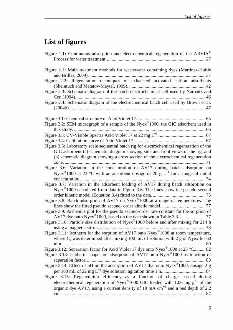
List of figures Figure 1.1: Continuous adsorption and electrochemical regeneration of the ARVIA®
Process for water treatment. .................................................................................... 27
Figure 2.1: Main treatment methods for wastewater containing dyes (Martínez-Huitle
and Brillas, 2009). ................................................................................................... 37
Figure 2.2: Regeneration techniques of exhausted activated carbon adsorbents (Sheintuch and Matatov-Meytal, 1999). ................................................................. 42
Figure 2.3: Schematic diagram of the batch electrochemical cell used by Narbaitz and Cen (1994). .............................................................................................................. 46
Figure 2.4: Schematic diagram of the electrochemical batch cell used by Brown et al. (2004b). ................................................................................................................... 47
Figure 3.1: Chemical structure of Acid Violet 17. .......................................................... 65
Figure 3.2: SEM micrograph of a sample of the Nyex®1000, the GIC adsorbent used in this study. ................................................................................................................ 66
Figure 3.3: UV-Visible Spectra Acid Violet 17 at 22 mg L−1. ....................................... 67
Figure 3.4: Calibration curve of Acid Violet 17. ............................................................ 67
Figure 3.5: Laboratory scale sequential batch rig for electrochemical regeneration of the GIC adsorbent (a) schematic diagram showing side and front views of the rig, and (b) schematic diagram showing a cross section of the electrochemical regeneration zone. ........................................................................................................................ 71
Figure 3.6: Variation in the concentration of AV17 during batch adsorption on Nyex®1000 at 23 °C with an adsorbent dosage of 20 g L−1 for a range of initial concentration. .......................................................................................................... 74
Figure 3.7: Variation in the adsorbent loading of AV17 during batch adsorption on Nyex®1000 calculated from data in Figure 3.6. The lines show the pseudo second order kinetic model (Equation 3.4) fitted to the data. ............................................. 75
Figure 3.8: Batch adsorption of AV17 on Nyex®1000 at a range of temperatures. The lines show the fitted pseudo second- order kinetic model. ..................................... 77
Figure 3.9: Arrhenius plot for the pseudo second-order rate constant for the sorption of AV17 dye onto Nyex®1000, based on the data shown in Table 3.3. ...................... 77
Figure 3.10: Particle size distribution of Nyex®1000 before and after mixing for 214 h using a magnetic stirrer. .......................................................................................... 78
Figure 3.11: Isotherm for the sorption of AV17 onto Nyex®1000 at room temperature, where Ce was determined after mixing 100 mL of solution with 2 g of Nyex for 60 min. ......................................................................................................................... 80
Figure 3.12: Separation factor for Acid Violet 17 dye onto Nyex®1000 at 23 °C.......... 82
Figure 3.13: Isotherm shape for adsorption of AV17 onto Nyex®1000 as function of separation factor. ..................................................................................................... 83
Figure 3.14: Effect of pH on the adsorption of AV17 dye onto Nyex®1000, dosage 2 g per 100 mL of 22 mg L−1 dye solution, agitation time 1 h. ..................................... 84
Figure 3.15: Regeneration efficiency as a function of charge passed during electrochemical regeneration of Nyex®1000 GIC loaded with 1.06 mg g−1 of the organic dye AV17, using a current density of 10 mA cm−2 and a bed depth of 2.2 cm. ........................................................................................................................... 87

List of figures
7
Figure 3.16: Five stage adsorption/regeneration performance system for Acid Violet 17 at initial concentration 668 mg L−1, using Nyex®1000 adsorbent with a dosage of 125 g L−1. ................................................................................................................ 88
Figure 3.17: AV17 and COD concentrations for five stages of adsorption / regeneration for an initial AV17 concentration of 668 mg L−1. ................................................... 89
Figure 3.18: Schematic diagram of multi-stage adsorber and regeneration system. ...... 92 Figure 3.19: Amount of adsorbent required per unit volume of effluent treated against
the percentage removal at different initial dye (AV17) concentrations for a five stage batch adsorption and regeneration system. .................................................... 95
Figure 3.20: performance of the batch adsorption and electrochemical regeneration system for removal of AV17 using Nyex®1000 with five stages adsorption and regeneration. ............................................................................................................ 96
Figure 3.21: Effect of the adsorptive capacity (kL) on the number of stages required for 99.9% removal of AV17 (with an initial concentration of 1 g L−1) using multi-stage adsorption-regeneration........................................................................................... 97
Figure 4.1: Airlift reactors: (a) the four main types of internal air loop reactor: (i) split
cylinder, (ii) concentric draught-tube and (iii) single-annulus, (iv) multiple-annulus; and (b) external loop airlift reactor. ........................................................ 104
Figure 4.2: Schematic diagram showing side and top views of a three compartment multiple airlift reactor (Bakker et al., 1993). ........................................................ 106
Figure 4.3: Split-cylinder airlift reactor used for the adsorption of a reactive dye on chitosan (Filipkowska and Waraksa, 2008). ......................................................... 107
Figure 4.4: Real flow patterns exist in process equipment (Levenspiel, 1999). .......... 110
Figure 4.5: Various tracer injection – response RTD measurements techniques (Fogler, 1999). .................................................................................................................... 113
Figure 4.6: (a) Schematic diagram and (b) annotated photograph of the smaller air lift reactor for continuous water treatment by adsorption with electrochemical regeneration. .......................................................................................................... 124
Figure 4.7: (a) Schematic diagram and (b) annotated photograph of the larger air lift reactor for continuous water treatment by adsorption with electrochemical regeneration. .......................................................................................................... 125
Figure 4.8: Schematic diagram of the electrochemical regeneration zone for (a) and (b) showing a cross section through line A-A in Figure 4.6 and 4.7, respectively. .... 126
Figure 4.9: Schematic diagram of the experimental setup for RTD and continuous adsorption and electrochemical regeneration experiments with the small unit. ... 128
Figure 4.10: Calibration curve for the conductivity of aqueous solutions of sodium chloride at a range of concentrations. ................................................................... 128
Figure 4.11: Schematic diagram of the bed movement experiment for the large unit. . 131 Figure 4.12: Stability of sodium chloride in the adsorption process for different dosage
of GIC adsorbent of 10 and 20 g L−1 and an initial concentration of NaCl tracer of 5350 mg L−1. ......................................................................................................... 132
Figure 4.13: The measured exit age distribution for the small continuous treatment unit. The exit age distribution obtained using the tank in series model for values of nT of 1, 2 (Equation 4.32) and 1.11 (Equation 4.36) is also shown. .............................. 134
Figure 4.14: Tank in series response to a pulse inert tracer experiment for different nT (Equation 4.32). ..................................................................................................... 135
Figure 4.15: Comparison between the tanks in series and closed dispersion models at
dimensionless variance 5.02 =θσ corresponding to nT =2 and Pe = 2.557. ........... 136

List of figures
8
Figure 4.16: Comparison of the closed dispersion model (Equation 4.27 fitted to the experimental data with Pe = 0.43 at dimensionless variance 87.02 =θσ ) with the
measured exit age distribution for the small continuous treatment process.......... 136
Figure 4.17: Schematic diagram showing the air nozzle locations with respect to the downcomer of the large unit (all dimensions in cm)............................................. 138
Figure 4.18: Effect of the air injection rate to nozzle I2 on the bed velocity for a total air injection rate of 15.5 L min-1 in each side under different air configuration and water flow rate. The bed velocity was taken from the average of three measurements and the error bars show the standard deviation of the three measurements in each case.................................................................................... 139
Figure 4.19: Schematic diagram showing the air nozzle locations with respect to the downcomer of the small unit (all dimensions in cm). ........................................... 139
Figure 4.20: Adsorbent concentration in the adsorption zone of the Arvia® Process large unit at different air configuration supply to the outer nozzles I4, 5 and 6 with different water flow rate. The adsorbent concentration was taken from the average of three measurements and the error bars show the standard deviation of the three measurements in each case.................................................................................... 140
Figure 4.21: Schematic diagram of the experimental set up for continuous water treatment using the large unit. ............................................................................... 144
Figure 4.22: Reactor large unit response to a step input of AV17 in the absence of adsorbent, where the inlet concentration of AV17 was increased from zero to 27 mg L−1 at t = 0, with a feed flow rate of 0.75 L min−1. ......................................... 146
Figure 4.23: Reactor response for adsorption of AV17 onto Nyex®1000 with no regeneration in the Arvia® process large unit. ...................................................... 148
Figure 4.24: Estimated actual loading from experimental data for AV17 on the adsorbent in the adsorption zone. The loading was calculated from the concentration data shown in Figure 4.23 using a numerical integration of Equation 4.41. ....................................................................................................................... 149
Figure 4.25: Reactor performance for adsorption and regeneration at various influent flow rates in the Arvia® large unit. ....................................................................... 151
Figure 4.26: Reactor performance for adsorption and regeneration at different initial concentration in the Arvia® large unit. .................................................................. 151
Figure 4.27: Estimated loading of AV17 on the adsorbent in the adsorption zone for various values of the feed flow rate. The loading was calculated from the concentration data shown in Figure 4.25 using a numerical integration of Equation 4.46. ....................................................................................................................... 153
Figure 4.28: Estimated loading of AV17 on the adsorbent in the adsorption zone for various values of the feed concentration. The loading was calculated from the concentration data shown in Figure 4.26 using a numerical integration of Equation 4.46. ....................................................................................................................... 154
Figure 4.29: Process response for adsorption of AV17 with / absence regeneration in the large cell process at flow rate 0.75 L min−1. ......................................................... 155
Figure 4.30: Schematic diagram of the processes occurring in the continuous adsorption with no regeneration adsorber. .............................................................................. 157
Figure 4.31: Schematic diagram of the processes occurring in the continuous adsorption with electrochemical regeneration reactor. ........................................................... 160
Figure 4.32: Comparison of the outlet concentration (Cout) predicted by numerical integration of Equations (4.49) and (4.51) with the experimental data for continuous adsorption with no regeneration with Q = 0.75 L min−1 feed flow rate

List of figures
9
and Cin = 107 mg L−1 inlet concentration. The dashed line shows the predicted outlet concentration in the absence of adsorbent, obtained by setting k2 = 0 (Equation 4.38). ..................................................................................................... 165
Figure 4.33: Comparison of the outlet adsorbent loading (qout) predicted by numerical integration of Equations (4.49) and (4.51) with the values estimated from the experimental data for continuous adsorption with no regeneration with Q = 0.75 L min−1 feed flow rate and Cin = 107 mg L−1. The red line shows the best fit at an adjusted k2 value of 0.7 g mg−1 min−1. .................................................................. 166
Figure 4.34: Comparison of the loading of the adsorbent leaving the adsorption zone (qout) calculated by numerical integration of Equations (4.49) and (4.51) and the loading of the adsorbent entering the adsorption zone (qin) determined from Equations (4.52) and (4.53), for the case of continuous adsorption with no regeneration. .......................................................................................................... 166
Figure 4.35: Measured concentrations of adsorbent in the adsorption zone of the large unit at a range of feed flow rate. The line shows the linear relationship (Equation 4.76) fitted to the data by linear regression. .......................................................... 168
Figure 4.36: Variation of the calculated values of Cout and qout (determined by numerical integration of Equations 4.49 and 4.51) after 300 min of continuous adsorption with no regneration for a range of feed flow rates Q at a feed concentration of 107 mg L−1. .................................................................................................................. 169
Figure 4.37: Variation of the percentage removal with feed flow rate based on the data shown in Figure 4.36. ............................................................................................ 169
Figure 4.38: Variation of the calculated values of Cout and qout (determined by numerical integration of Equations 4.49 and 4.51) after 300 min of continuous adsorption with no regneration for a range of feed concentration Cin and at a feed flow rate of 0.75 L min−1. ......................................................................................................... 170
Figure 4.39: Variation of the calculated values of Cout and qout (determined by numerical integration of Equations 4.49 and 4.51) after 300 min of continuous adsorption with no regneration for a feed flow rate of 0.75 L min−1 and inlet concentration of 107 mg L−1. ........................................................................................................... 171
Figure 4.40: Comparison of the percentage removal predicted from the numerical solution to Equation (4.56) with the experimental values obtained for continuous adsorption and electrochemical regeneration process in the large unit. A range of inlet concentrations of AV17 and solution flow rates were used, as discussed in section 4.3.3.3. The larger open symbols indicate the experimental data, while the smaller filled symbols show the predicted removal based on Equation (4.56). .... 172
Figure 4.41: Comparison of the percentage removal predicted from the numerical solution to Equation (4.56) with the experimental values obtained for continuous adsorption and electrochemical regeneration process in the small unit. A range of inlet concentrations of AV17 and solution flow rates were used, as described in Mohammed et al. (2011), see Appendix F. The larger open symbols indicate the experimental data, while the smaller filled symbols show the predicted removal based on Equation (4.56)....................................................................................... 172
Figure 4.42: Comparison of the predicted and measured variation of the outlet concentration (Cout) for continuous adsorption with electrochemical regeneration for a range of inlet concentrations at 0.6 L min−1 feed flow rate in the larger unit. The symbols indicate the experimental data for several inlet concentrations: (+) 80; (*) 140; and (o) 153 mg L−1, while the solid line shows the predicted outlet

List of figures
10
concentration determined by numerical integration of Equations (4.49) and (4.58). ............................................................................................................................... 173
Figure 4.43: Comparison of the predicted outlet loading (qout) with that determined from the experimental measurements for continuous adsorption with electrochemical regeneration for a range of inlet concentrations at 0.6 L min−1 feed flow rate in the larger unit. The symbols indicate the experimental data for several inlet concentrations: (+) 80; (*) 140; and (o) 153 mg L−1, while the solid lines show the predicted outlet loading determined by numerical integration of Equations (4.49) and (4.58). ............................................................................................................. 174
Figure 4.44: Comparison of the predicted and measured variation of the outlet concentration (Cout) for continuous adsorption with electrochemical regeneration process for a range of feed flow rate at 99 mg L−1 inlet concentration in the larger unit. The symbols indicate the experimental data for several of feed flow rates: (o) 0.25; (+) 0.5; and (*) 0.75 L min−1, while the solid line show the predicted outlet concentration determined by numerical integration of Equations (4.49) and (4.58). ............................................................................................................................... 175
Figure 4.45: Comparison of the predicted outlet loading (qout) with that determined from the experimental measurements for continuous adsorption with electrochemical regeneration for a range of feed flow rates at 99 mg L−1 inlet concentration in the larger unit. The symbols indicate the experimental data for several of feed flow rates: (o) 0.25; (+) 0.5; and (*) 0.75 L min−1, while the solid line show the predicted outlet loading determined by numerical integration of Equations (4.49) and (4.58). ............................................................................................................. 175
Figure 4.46: Percentage removal and normalised outlet adsorbent loading calculated for the continuous process of adsorption with regeneration with an adsorption zone that behaves as a CSTR (using Equation 4.56) for a range of feed flow rates, with an inlet concentration of 100 mg L−1 and a volume of reactor of 36 L. Other parameters are given in Table 4.4. ........................................................................ 176
Figure 4.47: Percentage removal and normalised outlet adsorbent loading calculated for the continuous process of adsorption with regeneration with an adsorption zone that behaves as a CSTR (using Equation 4.56) for a range of adsorption zone volumes, a feed flow rate of 0.6 L min−1 and an inlet concentration of 100 mg L−1. Other parameters are given in Table 4.4. .............................................................. 177
Figure 4.48: Schematic diagram of PFR ....................................................................... 178
Figure 4.49: Comparison of co-current PFR and CSTR systems for percentage removal of AV17 by continuous adsorption with regeneration at a feed concentration of 100 mg L−1 and an adsorption zone volume of 36 L. ................................................... 181
Figure 4.50: Comparison of co-current PFR and CSTR adsorption systems for rate removal of AV17 (mg min−1) for continuous adsorption with regeneration at a feed concentration of 100 mg L−1 and a volume of 36 L. ............................................. 181
Figure 4.51: Comparison of PFR and CSTR model to percentage removal of AV17 for adsorption and electrochemical regeneration at a feed concentration of 100 mg L−1 and a feed flow of 0.6 L min−1. ............................................................................. 182
Figure 4.52: Calculated percentage removal of AV17 achieved with n CSTR continuous adsorption with regeneration systems in series for an inlet concentration 100 mg L−1, a feed flow rate of 1 L min−1, and a fixed total adsorption zone volume of nV = 36 L. ...................................................................................................................... 183
Figure 4.53: Effect of adsorptive capacity (kL) on the number of CSTRs required to achieve 99% removal of AV17 (with an initial concentration of 100 mg L−1) for

List of figures
11
continuous adsorption with regeneration at a flow rate of 1 L min−1, and a fixed total adsorption zone volume of nV = 36 L. .......................................................... 184
Figure A.1: UV-Visible spectra of Acid Violet 17 at different pH. .............................. 212
Figure B.1: The measured exit age distribution for the multi-cell continuous treatment
process. The exit age distribution obtained using the tank in series model for the value of nT of 2 (Equation 4.32) and 1.137 (Equation 4.36) is also shown. ......... 216
Figure B.2: Schematic diagram of the experimental setup for multi-cell continuous adsorption and electrochemical regeneration and RTD experiments. .................. 216
Figure B.3: Reactor performance for adsorption and regeneration at various currents supplied in the Arvia multi-cell unit. .................................................................... 217
Figure E.1: Outlet concentration predicted, Cout for the adsorption with regeneration
model at flow rate of 0.6 L min−1 using a step size, h = 0.001 and 10. ................. 233
Figure E.2: Outlet loading predicted, qout for the adsorption with regeneration model at flow rate of 0.6 L min−1 using a step size, h = 0.001 and 10. ............................... 233
Figure E.3: Outlet concentration predicted, Cout for the adsorption with no regeneration model at flow rate of 0.75 L min−1 and feed concentration of 107 mg L−1 using a step size, h = 0.06 and 0.001. ................................................................................ 234
Figure E.4: Outlet loading predicted, qout for the adsorption with no regeneration model at flow rate of 0.75 L min−1 and feed concentration of 107 mg L−1 using a step size, h = 0.06 and 0.001. ....................................................................................... 234
Figure E.5: Outlet concentration predicted, Cout for the PFR model at feed flow rate of 1 L min−1 and feed concentration of 100 mg L−1 using a step size, h = 0.06 and 0.001. ............................................................................................................................... 235
Figure E.6: Outlet loading predicted, qout for the PFR model at feed flow rate of 1 L min−1 and feed concentration of 100 mg L−1 using a step size, h = 0.06 and 0.001. ............................................................................................................................... 235

List of tables
12
List of tables Table 2.1: Chemical groups and classification of chromophores and auxochromes
(Rangnekar and Singh, 1980) .................................................................................. 32
Table 2.2: Usage classification dye method (Hunger, 2003); and (Rangnekar and Singh, 1980). ...................................................................................................................... 34
Table 2.3: Characteristics of different types of adsorbent (Cooney, 1999); (Christy, 2008); (Doraiswamy, 2001); (Letterman, 1999); and (Robinson et al., 2001) ....... 39
Table 2.4: Physical and electrochemical properties of adsorbent (Cooney, 1999); (Brown et al., 2004a); (Wissler, 2006); (Asghar, 2011). ........................................ 40
Table 2.5: Comparative cost for different adsorbent regeneration techniques. .............. 48
Table 2.6: Advantages and disadvantages of some treatment methods for wastewater containing dye (Mahmoud et al., 2007); (Allègre et al., 2006); (Joshi and Purwar, 2004). ...................................................................................................................... 52
Table 3.1: Effect of separation factor on isotherm shape................................................ 58
Table 3.2: Kinetic rate constants for the adsorption of AV17 onto Nyex®1000 dose 20 g L−1, where qe1 and qe2 are the fitted equilibrium loadings for the first order and second order models respectively. .......................................................................... 75
Table 3.3: Parameters obtained for the pseudo second-order model fitted to the adsorption data plotted in Figure 3.8 at a range of temperature and 22 mg L−1 initial dye concentration of AV17. .................................................................................... 76
Table 3.4: Langmuir, Freundlich and Redlich-Peterson isotherm constants for sorption of Acid Violet 17 onto Nyex®1000, dosage 2 g/100 mL. ....................................... 79
Table 3.5: comparison of Langmuir constants and surface area for adsorption of methylene blue (MB), and AV17 onto various activated carbon (El Qada et al., 2008) and Nyex®1000 (from this work), respectively, at room temperature and normal pH. .............................................................................................................. 81
Table 3.6: Five stages adsorption/regeneration process for AV17 onto Nyex®1000, dosage 125 g L−1 at room temperature. ................................................................... 88
Table 4.1:Tracer types employed in air water system and detection devices (Shah,
1979). .................................................................................................................... 111
Table 4.2: Percentage removal of AV17 at different flow rate and initial concentration for adsorption and regeneration process. .............................................................. 150
Table 4.3: Values of the parameters m• and m used to calculate qout from the outlet experimental concentration (Cout). ........................................................................ 152
Table 4.4: Values of the parameters used in the model. ............................................... 164
Table 4.5: Values of parameters for the measured and predicted concentrations in the adsorption zone at different feed flow rate. .......................................................... 167
Table A.1: Effect of AV17 concentration on uptake by Nyex®1000, dosage 20 g L−1. 210
Table A.2: Effect of AV17 temperature on uptake by Nyex®1000, dosage 20 g L−1. .. 211 Table A.3: Relationship between isotherm equilibrium AV17 concentrations (Ce) and
uptake by Nyex®1000 (qe) dosage 20 g L−1. ......................................................... 211
Table A.4: Effect of pH of adsorption of AV17 onto Nyex®1000 at initial concentration of 22 mg L−1 and dosage 20 g L−1. ........................................................................ 212

List of tables
13
Table A.5: Effect of charge passed on the batch adsorption – electrochemical regeneration efficiency of AV17 onto Nyex®1000 at initial concentration of 120 mg L−1 and dosage of 100 g L−1. ........................................................................... 213
Table B.1: RTD test in the single cell small unit by injection of a pulse of NaCl solution
(26w %) at 320 mL min−1water flow rate. ............................................................ 214
Table B.2: RTD test in the multi-cell unit by injection of a pulse of NaCl solution (26w %) at 5.5 L min−1 water flow rate. ......................................................................... 215
Table B.3: Effect of initial concentration on the performance of the Arvia single-cell large unit for adsorption with electrochemical regeneration at feed flow rate of 0.6 L min−1. ................................................................................................................. 218
Table B.4: Effect of feed flow rate on the performance of the Arvia single-cell large unit for adsorption with electrochemical regeneration at initial concentration of around 100 mg L−1. ........................................................................................................... 219
Table B.5: Reactor performance for adsorption with no regeneration (no current supplied) at feed flow rate of 0.75 L min−1 and feed concentration of around 107 mg L−1 in the Arvia single cell large unit. ............................................................. 220
Table B.6: Reactor performance in the absence of adsorbent at feed flow rate of 0.75 L min−1 and feed concentration of 27 mg L−1 in the Arvia single cell large unit. .... 220
Table B.7: Nozzle configuration and air flow rates for the adsorbent circulation experiments. .......................................................................................................... 221
Table B.8: Effect of water flow rate on the bed velocity in the Arvia single cell large unit. ....................................................................................................................... 221
Table B.9: Standard deviations for the experimental data are shown in Table B.8. ..... 221
Table B.10: Adsorbent concentration in the adsorption zone of the Arvia single cell large unit at different water flow rates and air configurations. ............................. 222

Abstract
14
ABSTRACT
This thesis describes both batch and continuous processes for water treatment by adsorption with electrochemical regeneration of the adsorbent using an airlift reactor. The process is based on the adsorption of dissolved organic pollutants onto a graphite intercalation compound (GIC) adsorbent and subsequent electrochemical regeneration of the adsorbent by anodic oxidation of the adsorbed pollutant. Batch experiments were carried out to determine the adsorption kinetics and equilibrium isotherm for a sample contaminant, the organic dye Acid Violet 17 on the GIC (Nyex®1000) adsorbent. The adsorption capacity was found to be around 1 ± 0.05 mg g−1. The rate of adsorption appeared to follow pseudo-second order kinetics. The increase in the rate adsorption with temperature indicated an activation energy of around 4.2 KJ mole−1, suggesting that the mechanism of adsorption was physisorption. It was demonstrated that the adsorbent could be regenerated by anodic oxidation of the adsorbed dye in a simple electrochemical cell. The GIC adsorbent recovered its initial adsorption capacity after 40 to 60 min of treatment at a current density of 10 mA cm−2, corresponding to a charge passed of 12 to 15 C g−1 of adsorbent. The charge passed is consistent with that expected for mineralisation of the dye suggesting that the dye was removed and destroyed with high charge efficiency. Experiments were carried out to investigate the characterisation and performance of the continuous process, where water is treated continuously in a fluidised adsorption zone and the adsorbent is circulated through a moving bed electrochemical regeneration cell. The adsorbent circulation rate, the residence time distribution (RTD) of the reactor, and water treatment performance by continuous adsorption and electrochemical regeneration were studied. The RTD behaviour could be approximated as a continuously stirred tank. It was found that greater than 90% removal at feed concentrations of up to 100 mg L−1 were achieved using a single pass through a large continuous treatment unit by adsorption and electrochemical regeneration with a flow rate of 0.25 L min−1. In a smaller continuous treatment unit 98% removal at feed concentrations of up to 66 mg L−1 were achieved in a single pass with a flow rate of 0.24 L min−1. Steady state and dynamic models have been developed for the continuous process performance, assuming full regeneration of the adsorbent in the moving bed electrochemical cell. Experimental data and modelled predictions (using parameters for the adsorbent circulation rate, adsorption kinetics and isotherm obtained experimentally) of the dye removal achieved were found to be in good agreement. A higher dye removal was found with a co-current PFR model, but a number of tank in series (n CSTRs) was found to give higher contaminant removal for the same total adsorption zone volume. It was also found that the predicted number of stages of batch adsorption / regeneration required to achieve 99.9% AV17 removal was halved when the adsorptive capacity of the adsorbent was doubled. Similarly the predicted number of continuous CSTR adsorption / electrochemical regeneration process units required in series to achieve 99% AV17 removal was reduced by more than two thirds when the adsorptive capacity of the adsorbent was doubled.

Declaration
15
Declaration
No portion of the work referred to in this thesis has been submitted in support of an
application for another degree or qualification of this or any other university or other
institute of learning.
Fadhil Muhi Mohammed
June 2011

Copyright statement
16
Copyright statement
i. The author of this thesis (including any appendices and/or schedules to this thesis) owns certain copyright or related rights in it (the “Copyright”) and he has given The University of Manchester certain rights to use such Copyright, including for administrative purposes.
ii. Copies of this thesis, either in full or in extracts and whether in hard or
electronic copy, may be made only in accordance with the Copyright, Designs and Patents Act 1988 (as amended) and regulations issued under it or, where appropriate, in accordance with licensing agreements which the University has from time to time. This page must form part of any such copies made.
iii. The ownership of certain Copyright, patents, designs, trade marks and other
intellectual property (the “Intellectual Property”) and any reproductions of copyright works in the thesis, for example graphs and tables (“Reproductions”), which may be described in this thesis, may not be owned by the author and may be owned by third parties. Such Intellectual Property and Reproductions cannot and must not be made available for use without the prior written permission of the owner(s) of the relevant Intellectual Property and/or Reproductions.
iv. Further information on the conditions under which disclosure, publication
and commercialisation of this thesis, the Copyright and any Intellectual Property and/or Reproductions described in it may take place is available in the University IP Policy (see http://www.campus.manchester.ac.uk/medialibrary/policies/intellectual-property.pdf.), in any relevant Thesis restriction declarations deposited in the University Library, The University Library’s regulations (see http://www.manchester.ac.uk/library/aboutus/regulations) and in The University’s policy on Presentation of Theses.

Dedication
17
Dedication To My mother, my wife and my lovely children Lujain, Zain Alabdeen, Arjiwan, and Mowej.

Acknowledgements
18
Acknowledgements I am highly indebted to my research supervisor, Dr E.P.L Roberts for his dedicated
assistance, consistent guidance, invaluable comments, suggestion and constructive
criticism throughout my research work. Special thank must go to Dr Andrew K.
Campen for his invaluable help in the experimental work carried out for this work.
Acknowledgements also go to ARVIA® Technology Ltd for allowing me to use the
facilities. I would like to thank Dr Nigel Brown, Mr David Sanderson, and Mr Donald
Eaton, for their kind help and for making this project feasible. Thanks to all staff,
friends and colleagues in the ARVIA research group. Special thanks Dr Nuria de las
Heras for her unconditional support during my PhD study.
I would like to acknowledge all members of School of Chemical Engineering and
Analytical Science (SCEAS). Thanks to the technicians in SCEAS especially Mr John
Riley, Mr Gary Burns, Mr Andrew Evans and others from SCEAS’s workshop for
technical support with the setup of the experiment.
My sincere gratitude goes to my sponsor Iraqi Ministry of Higher Education and
Scientific Research, Baghdad, Iraq, for their financial support.
Last but not least, my heartfelt thanks go to my mother for her assistance and prayer.
Special gratefulness goes to my wonderful wife, Mrs Zahra K. Aboud and my lovely
children for their encouragement, help, support and patience throughout my study
abroad, without them I would not be able to make it through.

List of symbols
19
List of symbols A Absorbance, arbitrary units
Ar Cross section area of the regeneration zone for continuous treatment
aR Redlich-Peterson constant model
b Langmuir constant related to the energy of adsorption
bR Redlich-Peterson constant model
C Dimensionless liquid concentration
Ce Equilibrium concentration
Cο Initial concentration
Cout Outlet concentration
Cin Inlet concentration
Cn Concentration at stage n for adsorption and regeneration process
Cv Concentration in dv
dv Differential volume element
D Longitudinal dispersion coefficient
E Activation energy of adsorption
Et Exit age distribution function
Eθ Normalised exit age distribution function
F Faraday’s constant, 96487 C mol−1
Ft Cumulative distribution function
h Step size of integration method
I Current
k Conductivity
k1 Pseudo first-order rate constant
k2 Pseudo second-order rate constant
ko Frequency factor
kF Empirical Freundlich constant
kL Langmuir constant related to the adsorbent capacity
kR Redlich-Peterson constant model
l Path length through the sample, 1 cm
m Adsorbent concentration in the adsorption zone

List of symbols
20
m• Mass flow rate of adsorbent in the regeneration zone
M Total amount of adsorbent in the continuous treatment unit
Mw Molecular weight of the pollutant molecule
n Empirical Freundlich constant
nT Number of tank in series model
n Number of electrons required per molecules of pollutant oxidised
N Total mass of adsorbent in the regeneration zone
P Number of parameter in the isotherm equation
Pe Peclet number
q Dimensionless solid phase concentration
qi Adsorption capacity of fresh adsorbent
qin Adsorbent loading entering the adsorption zone
qe Equilibrium adsorbent loading
qe,m Experimental equilibrium adsorbent loading
qmx Maximum adsorbent loading leaving the adsorption zone
qout Adsorbent loading leaving the adsorption zone
qr Adsorption capacity of adsorbent after regeneration
qt Adsorbent loading at time t
qv Adsorbent loading in dv
Q Feed flow rate
rd Rate of adsorption per unit volume
R Universal gas constant, 8.314 J mol−1 k−1
R2 Coefficient of determination
RL Separation factor or equilibrium parameter
Rn Percentage removal at stage n for adsorption and regeneration process
S Skewness
tˊ Mean residence time
u Superficial fluid velocity
ur Bed velocity in regeneration zone for continuous water treatment
V Volume of the solution/adsorption zone
W Mass of adsorbent in the batch treatment unit

List of symbols
21
Greek scripts: αn Positive root of Equation 4.28
η Current efficiency
ηr Regeneration efficiency for adsorption and electrochemical regeneration
θc Normalized mean residence time for closed dispersion model
θo Normalized mean residence time for open dispersion model
θT Normalized mean residence time for tank in series model
σ Variance
τ Space time
List of abbreviations
22
List of abbreviations AC Activated carbon
ARE Average relative error
AV17 Acid Violet 17
BET Brunauer emmett teller
CAPEX Capital expenses
CFD Computational fluid dynamics
COD Chemical oxygen demand
CPC Cetyl pyridinium chloride
CSTER Continuous stirred tank electrochemical reactor
CSTR Continuous stirred tank reactor
DC Direct current
DSA Dimensionally stable anode
GAC Granular activated carbon
GIC Graphite intercalation compound
GRG Generalized reduced gradient
HDC Hydrodechlorination
HYBRID Hybrid fractional error function
LP Linear programming
MB Methylene blue
MIP Mixed integer optimization
MPSD Marquardt’s percent standard deviation
NF Nanofiltration
NLP Nonlinear optimization programming
ODE Ordinary differential equation
OPEX Operating expenses
PAC Powder activated carbon
PDE Partial differential equation
PFR Plug flow reactor
QP Quadratic programming
RB5 Reactive black 5
List of abbreviations
23
RE Regeneration efficiency
RO Reverse osmosis
RO16 Reactive orange 16
RTD Residence time distribution
SAE Sum of absolute errors
SEM Scanning electron microscope
SSE Sum of the squares of the errors
TC Theoretical charge
TDS Total dissolved solid
TOC Total organic carbon
TPM Tri-phenyl methane
WAO Wet air oxidation
WHO World health organization

Introduction Chapter 1
24
CHAPTER 1
INTRODUCTION
1.1 Background Dissolved organic pollutants such as dyes and pigments are considered one of the
problematic groups of pollutants as they are discharged into wastewaters from industrial
operations such as dye manufacturing, leather tanning, carpet, paper, food technology
and the textile industries. Many of these dyes are toxic and can be carcinogenic (McKay
et al., 1985). Therefore, it is necessary to remove them from liquid wastes to below the
concentrations accepted by national and international regulatory agencies before the
wastes are discharged to the environment. Removal of dye compounds can be difficult
and there are a number of processes used to reduce the concentration of dyes to the
limits recommended by the World Health Organization (WHO) including adsorption
(Walker and Weatherley, 2000), filtration (Mohan et al., 2002), chemical coagulation
(Vandevivere et al., 1998) and photo degradation (Chu and Ma, 2000). These processes
can be very effective for the removal of organic pollutants such as dyes, but have the
disadvantage that they produce secondary wastes.
Adsorption processes are an attractive approach for water treatment, particularly if the
adsorbent is cheap, does not require a pre-treatment step before its application and is
easy to regenerate (Wang et al., 2005). For many applications this process has proven to
be superior to other techniques for a variety of reasons (Sanghi and Bhattacharya,
2002); (Meshko et al., 2001); and (Bulut and Aydin, 2006), including the simplicity of
design, low cost, high removal efficiency, ease of operation and availability. One of the
most attractive processes is adsorption onto activated carbon as very low concentrations
at the outflow can be achieved and high loadings of pollutant are possible on these
adsorbents. Activated carbon adsorption has been widely investigated as the adsorbent
material to remove dyes from wastewater (Tunali et al., 2006); (Daifullah and Girgis,
1998); and (McKay et al., 1985). For example, Thinakaran et al. (2008) studied
adsorption of AV17 from aqueous solution onto activated carbon prepared from
sunflower seed hull. Adsorption processes are normally operated using a batch of

Introduction Chapter 1
25
adsorbent with sufficient capacity to operate for weeks or months before reaching
saturation. Once loaded the adsorbent must be disposed of or regenerated. The most
environmentally acceptable and cost effective approach is thermal regeneration (San
Miguel et al., 2001). However, analysis of the whole life costs of adsorption processes
indicates that most of the treatment costs are associated with regeneration (EPA, 1989).
In spite of this, most of the studies on adsorption have focused on the development of
adsorbents with high capacity and very few on developing adsorbents that can be easily
regenerated.
A search of the Science Citation Index for the last 20 years using the keywords
‘adsorbent’ and ‘capacity’ yields 3,654 references, while the keywords ‘adsorbent’ and
‘regeneration’ yields only 665 references.
1.2 Motivation
Recent work has shown that Nyex®, a graphite intercalation compound (GIC), which is
the subject of this study, is an effective adsorbent (albeit with relatively low capacity)
that can be electrochemically regenerated very rapidly and cheaply (Brown et al.,
2004a); (Brown et al., 2004b); (Brown et al., 2004c); (Brown, 2005). Adsorption on
Nyex® is rapid as it is non-porous, which eliminates intra-particle diffusion. GICs have
high electrical conductivity, associated with their graphitic nature, so that the energy
consumption during electrochemical regeneration is low. Based on these findings, a
continuous treatment process using Nyex® has been developed whereby continuous
adsorption and electrochemical regeneration occur within the same device (Brown et al.,
2007).
GICs are well known materials and their properties have been investigated (Enoki et al.,
2003). In GICs the intercalated molecules form layers in the Van der Waals gaps of the
graphite matrix. The use of such material for adsorption significantly reduces both the
time required to reach equilibrium, and the electrochemical regeneration time (Brown et
al., 2004a).
In this thesis, a GIC adsorbent, Nyex®1000, has been studied for the removal of a dye
(Acid Violet 17, AV17) from aqueous solution by both a batch and a continuous process
using adsorption and electrochemical regeneration (the ARVIA® process, described in
section 1.3). A chemical engineering model of the process has been developed for batch

Introduction Chapter 1
26
and continuous mode and these have been validated in a sequential batch cell and a
prototype device treating simulated waste water contaminated with an organic dye,
AV17, respectively. The design of any flow reactor depends upon two factors which are
the rate equations and backmixing or dispersion. In this case the first requires proper
mathematical representation of the amount of the contaminated adsorbate on the
adsorbent material at equilibrium and also requires a study of the kinetics of adsorption
to provide information about the mechanism of adsorption, which is important for the
efficiency of the process. The last factor is used to represent the combined action of all
phenomena, namely molecular diffusion, turbulent mixing, and non-uniform velocities,
which give rise to a distribution of residence time in the reactor (the residence time
distribution or RTD). The RTD can also be used to determine the mean residence time
and whether undesirable stagnant zones and / or by-pass routes occur within the reactor
(Levenspiel, 1999). A ‘tank in series’ or dispersion coefficient model are usually used to
express a mathematical description of RTD (Martin, 2000). Both a steady state and a
dynamic mathematical model for designing the ARVIA® treatment process, which is a
continuous stirred tank reactor (CSTR), have been developed for the process
performance of adsorption and electrochemical regeneration in continuous mode and
also in a plug flow reactor (PFR). A sensitivity study has been carried out for the PFR
and this is compared with the CSTR model at steady state. Also, a model of multi-stage
batch adsorption and regeneration has been developed and validated with experimental
data.
1.3 Introduction to the ARVIA ® Process A prototype wastewater treatment system has recently been developed in Manchester.
The University of Manchester spin-out ARVIA® Technology Ltd has been established
to commercialize this process. The process combines a novel adsorbent (Nyex®) and an
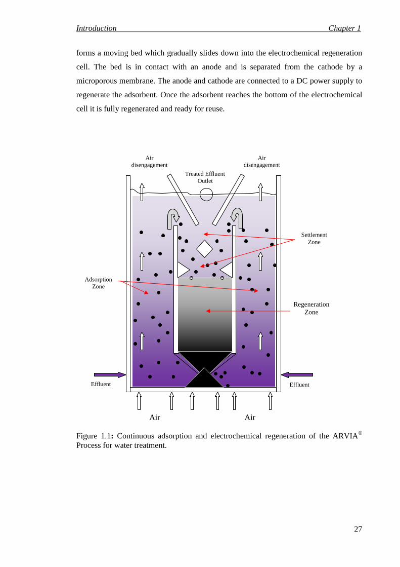
innovative electrochemical regeneration process. Figure 1.1, shows how the adsorbent is
circulated through adsorption and regeneration zones. The effluent is fed into the
adsorption zone and air is injected in order to fluidize the adsorbent and generate intense
mixing. The air is disengaged at the top of the adsorption zone and the adsorbent and
treated water flow into a settlement zone, where the adsorbent settle into the
regeneration zone and the treated water overflows out of the process. The adsorbent
Introduction Chapter 1
27
forms a moving bed which gradually slides down into the electrochemical regeneration
cell. The bed is in contact with an anode and is separated from the cathode by a
microporous membrane. The anode and cathode are connected to a DC power supply to
regenerate the adsorbent. Once the adsorbent reaches the bottom of the electrochemical
cell it is fully regenerated and ready for reuse.
Figure 1.1: Continuous adsorption and electrochemical regeneration of the ARVIA® Process for water treatment.
Settlement Zone
Air
Air disengagement
Air disengagement
Treated Effluent Outlet
Effluent Effluent
Air
Regeneration Zone
Adsorption Zone

Introduction Chapter 1
28
1.4 Scope of the work
This thesis focuses on development of a mathematical model of the batch and
continuous adsorption occurring in the ARVIA® process, which is a new development
in wastewater treatment based on the adsorption of organic pollutants (dyes) onto an
adsorbent material (Nyex®1000) and subsequent electrochemical regeneration of
adsorbent loaded with pollutant.
Accordingly, the main objectives of this thesis can be summarized as follows:
• Investigate equations which describe the adsorption of a typical organic dye,
including both the kinetic and equilibrium behaviour.
• Determine kinetic and equilibrium parameters using batch adsorption
experiments.
• Examine the effect of different parameters, such as temperature and pH on the
adsorption of dye.
• Investigate the electrochemical regeneration of Nyex®1000 loaded with dye and
the effect of the regeneration conditions on performance.
• Develop a design model for the treatment of water contaminated with dye using
multi-stage batch adsorption and electrochemical regeneration.
• Investigate the mixing behaviour in the continuous ARVIA® process using the
residence time distribution technique.
• Develop steady state and dynamic models for the continuous water treatment by
adsorption and electrochemical regeneration occurring in the ARVIA® process.
• Develop a dynamic model for the continuous water treatment by adsorption with
no regeneration occurring in the ARVIA® process.
• Develop a design model of water treatment by adsorption and electrochemical
regeneration with co-current plug flow of the adsorbent and water.
• Investigate the effect of operating conditions and key parameters on the process
performance using the model.

Introduction Chapter 1
29
This thesis is organized into five Chapters as follows:
Chapter 1 serves to introduce the problem and the objectives of the work.
Chapter 2 provides a review of the literature pertinent to this study, focussing on studies
of synthetic dyes and wastewater treatment methods. Dye classification methods are
reviewed according to the chemical structure and application or usage methods. Specific
topics covered include water treatment by adsorption processes and regeneration
methods with particular focus on electrochemical regeneration.
Chapter 3 discusses water treatment by batch adsorption and electrochemical
regeneration. Previous work in this area is discussed, including the theory related to the
kinetics and equilibrium of adsorption. The materials and methodology used are
described and experimental results for batch adsorption and electrochemical
regeneration are presented and discussed. A mathematical model of multi-stage
adsorption and regeneration is developed and validated.
Chapter 4 focuses on water treatment by continuous adsorption and electrochemical
regeneration. Relevant literature is reviewed, the behaviour of airlift reactors is
discussed and residence time distributions are explained. The experimental apparatus
and procedures for studying the continuous treatment process are described, including
the method used for measurement of the residence time distribution.
The methodology and the results of validation studies for modelling of continuous water
treatment by adsorption, and electrochemical regeneration are discussed. Sensitivity
studies to evaluate the effect of key parameters on performance are presented and
discussed.
Chapter 5 outlines the conclusions that can be drawn from this work and includes
suggestions and recommendations for future work.

Treatment of wastewater containing dyes Chapter 2
30
CHAPTER 2
TREATMENT OF WASTEWATER CONTAINING DYES
In this chapter, literature surveys on synthetic dyes and wastewater treatment methods
are described. The classification methods of dyes are introduced according to the
chemical structure and application or usage methods. The most common methods for
wastewater treatment are briefly described and special attention has been given to
adsorption and adsorbent regeneration processes for the treatment of wastewater
containing dye. Experimental methods described in the literature for adsorbent
regeneration are presented with some examples. A typical activated carbon adsorbent
has been compared for physical and electrochemical properties with the adsorbent that
was tested in this work (bisulphate GIC, Nyex®1000).
2.1 Synthetic dyes Over 700,000 tonnes dye stuff are produced annually estimated to consist of more than
100,000 commercially available dyes (Lee et al., 2006), (Forgacs et al., 2004). Mauveine
was the first modern synthetic organic dye discovered by chance by William Henry Perkin
in London in 1856 (McLaren, 1983). This product first sold under the name Tyrian
purple, but after 1859 was known as mauve and was made from coal tar. Actually, this
dye was neither the first synthetic dye to be produced in the laboratory nor even the first
to be manufactured. The first synthetic organic dye was picric acid, which had been
manufactured in 1845 by nitrating phenol (McLaren, 1983). Murexide was the second
synthetic dye which had been synthesised by Prout in 1818 but not exploited. He noted
its potential as a dyestuff and made it from nitric acid, uric acid and ammonia
(McLaren, 1983).
McLaren (1983) reports the first theory relating to chemical constitution and colour was
proposed by Graebe and Liebermann in 1868. This theory stated that as all known dyes
were decolorised on reduction, colour was associated with unsaturation. In 1875 the dye

Treatment of wastewater containing dyes Chapter 2
31
chemist Otto N. Witt proposed a colour theory and constitution that a compound is
coloured due to the presence of certain arrangements of atoms or groups, called
chromophores. Other groups called auxochromes enable the dye to bond to fibres and
modify the colour (Rangnekar and Singh, 1980).
A dye is a coloured compound used to impart its colour to a substrate material of which
it becomes an integral part by one of the various processes dyeing, printing, and surface
coating. Generally, the substrate includes textile fibres, polymers, foodstuffs, oils, leather,
and many other similar materials (Rangnekar and Singh, 1980).
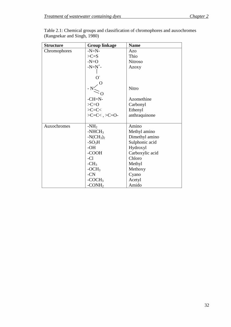
2.1.1 Dye chemistry The major components of dye molecules are chromophores and auxochromes. A
chemical structure which is coloured is normally accomplished in the synthesis of dyes
using a chromogen–chromophore with an auxochrome (Rangnekar and Singh, 1980).
The chromogen has an aromatic structure, i.e. it contains benzene, naphthalene, or
anthracene rings. The chromophore group is a ‘colour giver’ which forms a basis for the
chemical classification of dyes when coupled with the chromogen such as azo, carbonyl,
carbon- nitrogen, etc as shown in Table 2.1. The chromogen–chromophore structure is
often not sufficient to impart solubility and cause adherence of the dye to the fiber. The
word auxochrome is derived from two roots and the basic meaning of the auxochrome
is colour increaser. The prefix “auxo” means augment and the bonding affinity groups
are amine, hydroxyl, carboxyl, and sulphonic radicals or their derivatives.
Table 2.1 shows the classification of chromophores and auxochromes based on the key
chemical groups present. Dyes are normally classified based on the chromophores, e.g.
the azo, nitroso, nitro, thio, and carbonyl groups. In acid dyes the chromophores are part
of a negative ion, which are good for dyeing wool, acrylics, and silk, whereas in basic
dyes they are part of a positive ion used mostly for acrylics. Chromophores may contain
a chelate, which is a tightly bound metal in metallized dyes. Also, these groups are
important in vat, sulphur, disperse, direct, and reactive dye chemistry. The colour
produced by chromophores may be shifted or intensified by auxochrome groups such as
amino, halogen, alkoxyl, and hydroxyl groups.
Treatment of wastewater containing dyes Chapter 2
32
Table 2.1: Chemical groups and classification of chromophores and auxochromes (Rangnekar and Singh, 1980)
Structure Group linkage Name Chromophores -N=N-
>C=S -N=O -N=N+- O-
O - N O -CH=N- >C=O >C=C< >C=C< , >C=O-
Azo Thio Nitroso Azoxy Nitro Azomethine Carbonyl Ethenyl anthraquinone
Auxochromes -NH2 -NHCH3
-N(CH3)2
-SO3H -OH -COOH -Cl -CH3 -OCH3 -CN -COCH3 -CONH2
Amino Methyl amino Dimethyl amino Sulphonic acid Hydroxyl Carboxylic acid Chloro Methyl Methoxy Cyano Acetyl Amido

Treatment of wastewater containing dyes Chapter 2
33
2.1.2 Classification of dyes
There are two methods used to classify dyes, either according to their chemical structure
(particularly considering the chromophoric structure present in the dye molecule) or
according to how it is applied to the substrate (Hunger, 2003). The first method is
adopted by practising dye chemists and includes azo, anthraquinone, etc. dyes. The
latter method is adopted by the colour index.
2.1.2.1 Chemical structure method
The most appropriate way to classify dyes is by chemical structure which has many
advantages as follows (David and Geoffrey, 1990):
• It easily indentifies dyes as relating to a group which has characteristic
properties, for example azo dyes (strong, low cost) and anthraquinone dyes
(weak, expensive).
• There are a manageable number of chemical groups
In this method of classification, dye molecules are grouped to shared structural groups
(chromophoric structure) as shown in Table 2.1. For example, the azo dyes are the most
important class and contain at least one azo group (-N=N-) which is attached to two
radicals of which at least one but perhaps both are aromatic. The next most important
dye class contains carbonyl functions (-C=O) (Hunger, 2003).
2.1.2.2 Usage or application methods The classification of dyes by usage or application method is the principal approach
adopted by the colour index due to the fact that most textile fibers are polyester and
cotton. It is beneficial to consider this approach before the chemical structure method in
detail because of the dye nomenclature and jargon that arises from this approach. This
classification is listed in Table 2.2, which is organized according to colour index
application, shows the principal substrates, the methods of application, and the chemical
types of each class of dye.

Treatment of wastewater containing dyes Chapter 2
34
Table 2.2: Usage classification dye method (Hunger, 2003); and (Rangnekar and Singh, 1980).
Dye class Main application General description Chemical type
Reactive Used for all cellulosic goods (knitted fabric), wool, silk, and nylon
Easy application; moderate price, good fastness, anionic compounds, and highly water soluble
azo,anthraquinone, phthalocyanine, formazan, oxazine, and basic
Direct Cellulosic fibers, rayon, silk, and wool
Simple application, cheap, moderate colour fastness, anionic compounds, and highly water soluble
azo, phthalocyanine, stilbene, nitro, and benzodifuranone
Disperse Polyester, acetate, nylon, and acrylic
Require skill in application (by carrier or high temperature), good fastness, and limited solubility in water
azo, anthraquinone, styryl, nitro, and benzodifuranone
Acid Wool, silk, paper ink, nylon, and leather
Easy application, poor fastness, anionic compounds, and highly water soluble
azo (including premetallized), anthraquinone, azine, triphenylmethane, xanthene, nitro and nitroso
Basic Acrylic, polyester, wool, and leather
careful application required to prevent unlevel dyeing and adverse effect in hand feel, cationic, and highly water soluble
cyanine, azo, azine, hemicyanine, diazahemicyanine, triarylmethane, xanthen, acridine, oxazine, and anthraquinone
Vat Cotton (towel), wool, and rayon
Difficult to apply, expensive, good fastness except indigo and sulphurised vat species, and insoluble in water
anthraquinone (including polycyclic quinones) and indigoids
Mordant Wool products (carpet), leather, and anodized aluminium
Complicated application, expensive, good fastness, anionic compounds, and highly water soluble
azo and anthraquinone
Sulphur Used for heavy cellulose goods in dark shades, and rayon
Difficult to apply, cheap, poor fastness, and insoluble in water
indeterminate structures
Solvent Petroleum, plastic, wax and inks
Insoluble in water, fastness depend on material used on.
phthalocyanine, azo, anthraquinone and triphenylmethane

Treatment of wastewater containing dyes Chapter 2
35
Acidic dyes, which are the subject of this thesis (e.g. Acid Violet 17), have high water
solubility and a light fastness better than basic dyes. Acid dyes are used to dye or colour
paper, leather, ink-jet printing, food, and cosmetics. Moreover, they contain sulphonic
acid groups, which are usually present as sodium sulphonate salts, or carboxyl groups
making them soluble in water, and give the dye molecules a negative charge. In an
acidic solution, the -NH2 functionalities of the fibres are protonated to give a positive
charge: -NH3+. The interaction between this charge (positive) and the negative dye
charge, allows the formation of ionic interactions.
In this thesis Acid Violet 17 was selected as the model compound due to its low
toxicity, (some of the dye in the experiments was destined to be discharged to sewer)
and ready availability in relatively large quantities. It is a triphenylmethane dye
commonly used as a textile dye for dyeing wool, polyamide, nylon and silk and also for
non-textile applications on leather and anodised aluminium. Additionally, it has a use as
a stain for bacteria and cell cultures, (Venkataraman, 1952). It also has the advantage
that unlike azo dyes its breakdown products are not particularly hazardous, (azo dyes
can break down to regenerate the original amine which may be a carcinogen).
2.2 Wastewater treatment methods Pollution by organic chemicals including that by dyes is one of the most serious
environmental problems facing life on earth. There are several sources of water
pollution by dyes and pigments, such as leather tanning, paper, rubber, food technology
and the textile industry (Alkan et al., 2008). These dyes have a variety of complex
organic compounds and toxic substances with unknown environmental behaviour such
as aromatic amines (C6H5-NH2), which are suspected to have carcinogenic effect,
phenyl (C6H5-CH2) and naphthyle (NO2-OH) (McKay et al., 1985). The resistance of
these organic compounds to decomposition due to the complex chemical structure of
synthetic pigments in dyes results in a difficult to treat wastewater which is also
resistant to degradation by biological methods. These compounds are not removed
effectively by conventional physicochemical treatment methods such as sedimentation,
filtration, and coagulation/flocculation (Cooney, 1999).
Many researchers have studied different techniques to remove dyes from wastewater
including various chemical, physico-chemical and biological processes such as,
adsorption (Namasivayam and Kavitha, 2002); and (Nemr et al., 2009), chemical
Treatment of wastewater containing dyes Chapter 2
36
precipitation (Tan et al., 2000), electrochemical oxidation (Ahmed, 2008), nanofiltration
(Chakraborty et al., 2003), ultrafiltration (Ahmad et al., 2006), chemical oxidation
(ozonation) (Zhang et al., 2004, Konsowa, 2003), and aerobic and anaerobic biological
processes (An et al., 1996), (Isik and Sponza, 2006). Figure 2.1 summarized the main
techniques to remove dyes from wastewater.

Treatment of wastewater containing dyes Chapter 2
37
Figure 2.1: Main treatment methods for wastewater containing dyes (Martínez-Huitle and Brillas, 2009).
Physic-chemical methods
Chemical methods
Advanced oxidation processes
Adsorption
Coagulation
Filtration
Ion Exchange
Ozonation
Methods for dye removal from wastewaters
Hypochlorite ion
Fenton’s reagent (Fe2+/H2O2)
Photocatalysis - TiO2/UV - H2O2/UV - O3/UV
Microbiological treatments
Activated sludge processes
Mixed cultures - Aerobic decomposition - Anaerobic decomposition
Pure cultures - White-rot fungus - Bacteria
Enzymatic decomposition
Electrochemical methods
Electrocoagulation
Electrochemical reduction
Electrochemical oxidation
Indirect electro-oxidation with strong oxidants -chlorine -Fenton
Photoassisted electrochemical -Photoelectro -Fenton -Photoelectrocatalysis

Treatment of wastewater containing dyes Chapter 2
38
The most widely used methods are briefly described in the following sections:
2.2.1 Adsorption and regeneration processes 2.2.1.1 Adsorption
Among the unit operations in waste water treatment, adsorption occupies an important
position since it is an efficient and economically feasible process for treatment of
wastewater containing dissolved organic pollutants (Namasivayam and Kavitha, 2002);
(Nemr et al., 2009). In the adsorption process, molecules are extracted from one phase
(liquid phase, dye solution) and concentrated at the surface of a second phase (solid
phase, adsorbent) which occurs due to an attractive force existing between the adsorbent
surface and the adsorbate molecules. Therefore, it is a removal process where certain
molecules are bound to an adsorbent particle surface by either chemical or physical
attraction (described in section 2.2.1.3). The adsorption process consists of three
consecutive steps (Reynolds and Richards, 1996):
1. Substances adsorb to the exterior of the adsorbent
2. Substances move into the adsorbent pores
3. Substances adsorb to the interior walls of the adsorbent
2.2.1.2 Adsorbent types Virtually every solid surface has the capacity to adsorb sorbate but the effectiveness of
these solids in the wastewater treatment process is a function of its structure, degree of
polarity, porosity and specific area (Dechow, 1989). The adsorbate may be an organic
compound with undesirable properties such as colour, odour, etc. The principal types of
adsorbents include activated carbon, organic polymers and silica-based compounds and
examples are listed in Table 2.3.
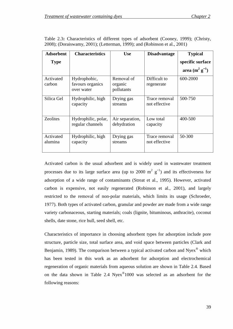
Treatment of wastewater containing dyes Chapter 2
39
Table 2.3: Characteristics of different types of adsorbent (Cooney, 1999); (Christy, 2008); (Doraiswamy, 2001); (Letterman, 1999); and (Robinson et al., 2001)
Adsorbent
Type
Characteristics Use Disadvantage Typical
specific surface
area (m2 g−−−−1)
Activated carbon
Hydrophobic, favours organics over water
Removal of organic pollutants
Difficult to regenerate
600-2000
Silica Gel Hydrophilic, high capacity
Drying gas streams
Trace removal not effective
500-750
Zeolites Hydrophilic, polar, regular channels
Air separation, dehydration
Low total capacity
400-500
Activated alumina
Hydrophilic, high capacity
Drying gas streams
Trace removal not effective
50-300
Activated carbon is the usual adsorbent and is widely used in wastewater treatment
processes due to its large surface area (up to 2000 m2 g−1) and its effectiveness for
adsorption of a wide range of contaminants (Streat et al., 1995). However, activated
carbon is expensive, not easily regenerated (Robinson et al., 2001), and largely
restricted to the removal of non-polar materials, which limits its usage (Schroeder,
1977). Both types of activated carbon, granular and powder are made from a wide range
variety carbonaceous, starting materials; coals (lignite, bituminous, anthracite), coconut
shells, date stone, rice hull, seed shell, etc.
Characteristics of importance in choosing adsorbent types for adsorption include pore
structure, particle size, total surface area, and void space between particles (Clark and
Benjamin, 1989). The comparison between a typical activated carbon and Nyex® which
has been tested in this work as an adsorbent for adsorption and electrochemical
regeneration of organic materials from aqueous solution are shown in Table 2.4. Based
on the data shown in Table 2.4 Nyex®1000 was selected as an adsorbent for the
following reasons:

Treatment of wastewater containing dyes Chapter 2
40
• The high density of Nyex® allows rapid settlement
• A tenfold increase in electrical conductivity of Nyex® aids electrochemical
regeneration
• Lack of Nyex® pores facilities more complete and rapid regeneration
• Lower surface area of Nyex® is compensated by continuous recycling and
regeneration.
However it should be noted that the low surface area of the Nyex®1000 means that it is
a low capacity adsorbent material.
Table 2.4: Physical and electrochemical properties of adsorbent (Cooney, 1999); (Brown et al., 2004a); (Wissler, 2006); (Asghar, 2011).
Characteristic Nyex®1000 Typical Activated Carbon Bulk density (g cm−3)
Particle density (g cm−3)
Real density (g cm−3)
0.4−0.5
0.5−0.6 (coal-based carbon) 0.24−0.3 (wood-based carbon)
0.74−0.8
2.1−2.2
Pore volume (cm3 g−1) 0 0.8−1.2 (coal-based carbon)
2.2−2.5 (wood-based carbon) Surface area (m2 g−1) 1.0 600−2000 Bed Electrical Conductivity (s cm−1)
0.8 0.025 (GAC)
0.016 (PAC) Resistivity (Ω cm) 1.25 39.45 (GAC)
85.11 (PAC)
2.2.1.3 Adsorption types
Adsorption is the phenomenon of accumulation of a large number of molecular species
at the surface of solid or liquid phase in comparison to the bulk. These phenomena can
be classified into two types depending on the nature of the bonding between the
molecules of the adsorbate and the surface of adsorbent, namely chemisorption and
physisorption. Both types take place when the molecules in the liquid phase (sorbate)
become attached to the surface of the solid phase (adsorbent) as a result of the attractive
forces at the adsorbent surface overcoming the kinetic energy of the adsorbate
molecules (Cheremisinoff, 2002).
Treatment of wastewater containing dyes Chapter 2
41
• Physisorption
Physisorption or physical adsorption occurs when, as a result of energy difference and /
or electrical attractive forces (weak Van der Waals forces), adsorbate molecules become
physically fastened to the adsorbent surface. Physisorption takes place with the
formation of single or multiple layers of adsorbate on the adsorbent surface and is
characterised by a low activation energy (enthalpy) of adsorption (20−40 KJ mol−1)
(Centrone et al., 2005).
• Chemisorption
Chemisorption or chemical adsorption occurs when a chemical reaction occurs between
the adsorbed molecules and the adsorbent. Chemisorption takes place with the
formation of a single layer of adsorbate attached to the adsorbent surface by chemical
bonds. This type of interaction is strong with a covalent bond between adsorbate and the
surface of the adsorbent is characterised by a high enthalpy of adsorption (200−400 KJ
mol−1).
2.2.1.4 Adsorbent regeneration and economics
Regeneration, or desorption is an important and necessary process when the adsorbent
used is expensive or if it is not always available in large quantities. Usually, this process
is achieved by changing the conditions in the adsorbent to bring about a lower
equilibrium loading capacity by increasing the temperature or decreasing the partial
pressure. From an economic view point, the sorbent can be considered effective if it can
be easily regenerated and reused as many times as possible without alteration of its
performance. There are several methods used for regeneration of adsorbent loaded with
organic pollutants materials. In practice, the choice of one type of regeneration process
versus another depends on many factors, such as cost, time, consumption and
regeneration efficiency. Activated carbon must be land filled, incinerated, or
regenerated for reuse after being exhausted or saturated with organic material. A
significant drawback of activated carbon is its high cost and the fact it is not easy to
regenerate. The cost of carbon regeneration has been estimated for commercial GAC at
about 75% of the maintenance and operation cost (EPA, 1989). There are several
methods for the regeneration of adsorbent loaded with organic materials. Figure 2.2
shows the different techniques that are available for regeneration of spent activated
carbon (Sheintuch and Matatov-Meytal, 1999).

Treatment of wastewater containing dyes Chapter 2
42
Thermal
Decomposition
Hot Water
Nonthermal
Steam
Electrochemical Microbial Chemical
Reduction Oxidation
Thermal Catalytic Catalytic
HDC Photocatalytic
Inert gas
Solvent extraction
Adsorbent
Desorption
Supercritical fluid extraction
Surfactant enhanced
Figure 2.2: Regeneration techniques of exhausted activated carbon adsorbents (Sheintuch and Matatov-Meytal, 1999).
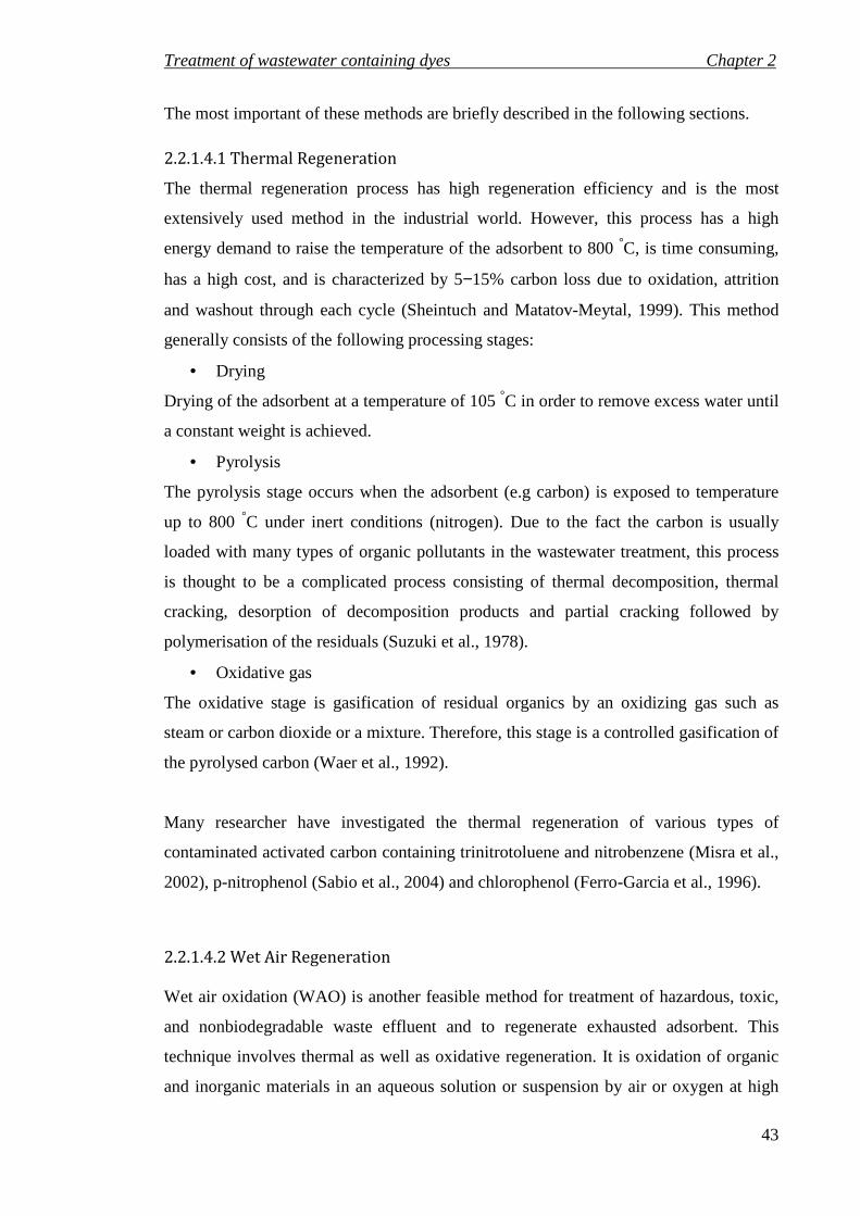
Treatment of wastewater containing dyes Chapter 2
43
The most important of these methods are briefly described in the following sections.
2.2.1.4.1 Thermal Regeneration
The thermal regeneration process has high regeneration efficiency and is the most
extensively used method in the industrial world. However, this process has a high
energy demand to raise the temperature of the adsorbent to 800 °C, is time consuming,
has a high cost, and is characterized by 5−15% carbon loss due to oxidation, attrition
and washout through each cycle (Sheintuch and Matatov-Meytal, 1999). This method
generally consists of the following processing stages:
• Drying
Drying of the adsorbent at a temperature of 105 °C in order to remove excess water until
a constant weight is achieved.
• Pyrolysis
The pyrolysis stage occurs when the adsorbent (e.g carbon) is exposed to temperature
up to 800 °C under inert conditions (nitrogen). Due to the fact the carbon is usually
loaded with many types of organic pollutants in the wastewater treatment, this process
is thought to be a complicated process consisting of thermal decomposition, thermal
cracking, desorption of decomposition products and partial cracking followed by
polymerisation of the residuals (Suzuki et al., 1978).
• Oxidative gas
The oxidative stage is gasification of residual organics by an oxidizing gas such as
steam or carbon dioxide or a mixture. Therefore, this stage is a controlled gasification of
the pyrolysed carbon (Waer et al., 1992).
Many researcher have investigated the thermal regeneration of various types of
contaminated activated carbon containing trinitrotoluene and nitrobenzene (Misra et al.,
2002), p-nitrophenol (Sabio et al., 2004) and chlorophenol (Ferro-Garcia et al., 1996).
2.2.1.4.2 Wet Air Regeneration Wet air oxidation (WAO) is another feasible method for treatment of hazardous, toxic,
and nonbiodegradable waste effluent and to regenerate exhausted adsorbent. This
technique involves thermal as well as oxidative regeneration. It is oxidation of organic
and inorganic materials in an aqueous solution or suspension by air or oxygen at high
Treatment of wastewater containing dyes Chapter 2
44
pressure (0.5–20 MPa) and temperature (125–320 oC) to enhance the solubility of
oxygen in the aqueous solution (Mishra et al., 1995). The advantages of this method for
regeneration of spent AC include (Knopp et al., 1978):
• Direct carbon slurry regeneration without dewatering.
• Absence of carbon particulate emissions.
• Carbon losses less than 7% due to no solid-liquid separation involved.
On the other hand, this method is very expensive because it requires large investment in
high pressure equipment and has a high running cost due to the elevated temperatures
and pressures.
2.2.1.4.3 Chemical Regeneration
Ferro-Garcia et al. (1996) investigated chemical regeneration as an alternative method
to thermal regeneration in which chemical reagents (solvent) are applied to the
exhausted carbon. When an adsorbent is chemically regenerated by treating with
methanol, acetone, ethanol and benzene, the amount of adsorbate removed has been
found to be a function of the accessibility of the organic regenerate and the adsorbate-
carbon surface interactions. The desorption or extraction of adsorbate is a simple and
inexpensive method. However, the regeneration efficiency (defined as the ratio of the
adsorption capacity after to before regeneration) of this method is usually below 70%
and about 10−15% of the AC pores are blocked by the solvent (Ferro-García et al.,
1993); (Martin and Ng, 1984); (Schweiger and Levan, 1993). Moreover, contaminant
materials are not destroyed, and the purification step for reuse of the solvent is
expensive. For these reasons, chemical regeneration is not widely used in practice.
However, the significant advantages of chemical / solvent regeneration of adsorbent
include (Cooney et al., 1983):
• Due to no adsorbent (carbon) loss during regeneration, the cost of carbon
attrition is avoided
• Due to the fact solvent regeneration can be done rapidly in situ, unloading,
transporting and repacking of adsorbents are eliminated.
• Is possible to recover valuable adsorbates (solute)
• Solvent can be reused easily by proper subsequent treatments such as
distillation.
• No degradation of the adsorbent surface or pore structure.

Treatment of wastewater containing dyes Chapter 2
45
Ferro-Garcia et al. (1996) found that the chemical regeneration of spent activated
carbons loaded with chlorophenols depended on the adsorbent porosity, the adsorbate-
adsorbent interactions and the nature of solvent used. The best solvent was ethanol and
orthochlorophenol could be extracted in a greater amount than metachlorophenol.
2.2.1.4.4 Electrochemical Regeneration
Electrochemical oxidation is considered a relatively new technique, developed in the
1990's and one which is becoming an alternative to thermal regeneration for wastewater
treatment, due to its capacity to clean the adsorbent and decompose the pollutant
(Narbaitz and Cen, 1994); (Narbaitz and Karimi-Jashni, 2009); (Zhou and Lei, 2006).
This technique possesses many potential advantages over thermal regeneration. These
include in situ regeneration, high regeneration efficiency, short time requirements,
minimal adsorbent losses, destruction of pollutants via oxidation at the anode, and
suitability for using small and medium sized treatment facilities (Berenguer et al.,
2010). Moreover, the proper setting of the current (or electrode potential) applied,
electrode composition, catholyte type and concentration, and electrolysis time can allow
for the conversion of organic pollutants into less hazardous compounds, or even
complete mineralization (Pletcher and Walsh, 1993); (Rajeshwar and Ibaner, 1996).
Electrochemical processes have been widely investigated for treating water
contaminated with organic pollutants (Panizza and Cerisola, 2001); (Panizza et al.,
2000); (Murphy et al., 1992) with significant interest being shown in the colour removal
from wastewater (Naumczyk et al., 1996); and (Vlyssides et al., 2000). The electrolytic
method that was examined gave a satisfactory result for colour removal from these
waste waters which were highly conductive due to the presence of NaCl that was used
as electrolyte. Electrochemical regeneration, which is the subject of this thesis, of
adsorbent loaded with organic materials has not been widely studied for the treatment of
wastewater. The first report on electrochemical regeneration of activated carbon was by
Owen and Barry (1972), who found regeneration efficiencies of up to 61% and
recommended that the process required further investigation. A number of other
researchers have investigated aspects of electrochemical regeneration of activated
carbon. Narbaitz and Cen (1994); Narbaitz and Karimi-Jashni (2009); and Zhang (2002)
have demonstrated regeneration of activated carbon loaded with phenol via batch
adsorption tests, achieving regeneration efficiencies (REs) of up to 95% in the cathode
compartment of the cell. Narbaitz and Cen (1994), whose apparatus is shown in Figure
Treatment of wastewater containing dyes Chapter 2
46
2.3, suggested that the electrochemical effects are restricted to the external surface of
the carbon and obtained best performance for regeneration at the cathode surface.
Figure 2.3: Schematic diagram of the batch electrochemical cell used by Narbaitz and Cen (1994).
However, the rate of adsorption and desorption of activated carbon is often governed by
intra particle diffusion and this requires long adsorption and regeneration times. Recent
work has shown that Nyex®, a GIC that is the subject of this thesis, is a non-porous
material and thus adsorption and regeneration is not controlled by intra-particle
diffusion. GIC’s are well known materials and their properties have been investigated
previously by Enoki et al. (2003). In GIC’s the intercalated molecules form layers in the
Van der Waals gaps of the graphite matrix. GIC’s have a high electrical conductivity, so
that energy consumption during electrochemical regeneration is low. Previous studies
have regenerated Nyex®100 a powdered GIC, Brown et al. (2004a); Brown et al.,
(2004b); and Brown et al. (2004c) in a batch cell shown schematically in Figure 2.4. In
this thesis, a flake GIC adsorbent with a larger particle size, Nyex®1000, has been
studied for the removal of a dye (Acid Violet 17, AV17) from aqueous solution. In
addition Nyex®1000 has been used in a continuous treatment process, whereby
continuous adsorption and electrochemical regeneration occur within the same device
Power Supply
Holder
Plexiglass ring
Electrolyte Anode
compartment
Cathode compartment
Platinum plates
- +

Treatment of wastewater containing dyes Chapter 2
47
(Brown et al., 2007). Nyex®1000 is more suitable than the powdered Nyex®100 for this
process application as it settles rapidly.
Figure 2.4: Schematic diagram of the electrochemical batch cell used by Brown et al. (2004b).
2.2.1.5 Summary of adsorbent regeneration techniques
The main techniques for regeneration of contaminated adsorbents including thermal,
wet air oxidation, chemical, and electrochemical methods have been summarised in this
section. A comparison of the total cost of these techniques, comprising both capital
expenses (CAPEX) and operating expenses (OPEX), is summarised in Table 2.5.
PVC Case
Anode
Cathode
Membrane
Catholyte
Nyex/electrolyte Mix
DC power Source
125-1000mA

Treatment of wastewater containing dyes Chapter 2
48
Table 2.5: Comparative cost for different adsorbent regeneration techniques.
Regeneration
technique
CAPEX OPEX Comments
Thermal
high relatively low high energy consumption
Electrochemical low high if AC is used and low using Nyex®1000
Chemical/Solvent high low but depends on requirement for solvent make up
solvent reuse requires a more expensive purification step
Wet air oxidation high relatively low
high energy consumption
All of these methods offer advantages and disadvantages, but only thermal regeneration
has been used commercially at large scale. It has been concluded that of the other
techniques available, anodic electrochemical regeneration has the most significant
potential, due to:
• Low energy consumption if graphite based adsorbents are used
• Operating conditions at ambient temperature and pressure
• In situ regeneration
• High regeneration efficiencies
• Low adsorbent losses during regeneration
• No contaminated waste is produced, due to destruction of contaminants on the
adsorbent surface via oxidation
• No sludge production
• Relatively simple process which is easy to operate and control.
Furthermore, the combination of electrochemical regeneration with graphite based
(GIC) adsorbents has recently been demonstrated commercially by Arvia® Technology
Ltd a spin-out company from the University of Manchester (Arvia® Technology Ltd.,
2010).

Treatment of wastewater containing dyes Chapter 2
49
2.2.2 Chemical oxidation
Chemical oxidation is frequently used in wastewater treatment using oxidants such as
chlorine (Cl2) and its derivatives (chlorine dioxide, sodium hypochlorite), hydrogen
peroxide (H2O2) (Collivignarelli and Bertanza, 1996), potassium permanganate
(KMnO4) (Xu et al., 2005), electrochemical oxidation, and ozone (O3) (Ciardelli and
Ranieri, 2001). Chemical oxidation can be used to destroy organic dyes, generating a
colourless solution. In decolourization, it has been shown to be very effective towards
acid, cationic and direct dyes while disperse and vat dyes were more resistant to ozone
treatment. The breakdown products from these processes can be removed by
conventional biological treatment. Ozone is one of the most powerful oxidizing agents
and produces nontoxic breakdown products which are converted to CO2 and H2O.
Ozone can be used for the treatment of drinking water to remove the unpleasant odour
and to inhibit the formation of halogenated products. The main purpose of ozonation in
water treatment is to achieve the following:
• Oxidation of organic micro-pollutants, e.g. odour compounds, taste, pesticides,
and phenolic pollutants.
• Oxidation of organic macro-pollutants, e.g. bleaching of colour.
• Oxidation of inorganic pollutants, e.g. manganese and iron.
• Enhancement of coagulation.
• Disinfection and algae control
2.2.3 Chemical precipitation
Chemical precipitation involves the addition of a reagent which reacts with the
dissolved organic materials and forms insoluble or sparingly soluble compounds; the
lower the solubility of the compound, the less organic material remains in the solution.
Settling, filtration or centrifugation can remove the precipitated materials in the form of
suspended solid particles. To enhance this settling and agglomeration of the suspended
solids, coagulants are often added (e.g. alum, poly aluminium chloride, and magnesium
chloride) that produce flocs which can collect dye molecules which can then be
separated from aqueous solution by means of physical sedimentation. Alum
(Al 2(SO4)3.H2O) is currently the most frequently used coagulant in water and
wastewater treatment due to its low cost and its proven performance in treatment
processes (Edzwald, 1993). Recently, poly aluminium chloride, which is a polymerised

Treatment of wastewater containing dyes Chapter 2
50
form of aluminium, has been widely investigated. This preformed polymeric aluminium
has some advantages over alum due to the partial elimination of the polymerisation
process that occurs after added the coagulant to the water (Van Benschoten and
Edzwald, 1990); (Viraraghavan and Wimmer, 1988). Magnesium chloride (MgCl2) is a
less commonly used coagulant in industrial wastewater treatment. Many applications
have been reported in which good coagulation could be achieved if enough magnesium
ions (Mg2+) were applied to the treatment unit by Tan et al. (2000) and Folkman and
Wachs (1973). Treatment by MgCl2 formed flocs which were found to give shorter
settling time than alum and poly aluminium chloride. This treatment was used by Tan
et al. (2000) on an industrial dye waste, and was found to give 98% colour removal, and
96% suspended solids removal.
However, the coagulation and flocculation process does not treat all dye types. Acid,
direct, vat, and reactive dyes coagulate well but the resulting flock is of a poor quality
and does not settle easily, while sulphur and disperse dyes coagulate well and settle
easily. Cationic dyes do not coagulate at all (Marmagne and Coste, 1996).
Generally, the disadvantages of chemical precipitation process include:
• A high mass of primary sludge is produced which must be disposed of and is
sometimes difficult to thicken and dewater.
• High operating costs of chemical addition.
• Not able to reduce the total dissolved solids (TDS).
2.2.4 Ultrafiltration
Ultrafiltration membrane technology has been applied in many industries, but it has not
been accepted widely in textile effluent treatment due to the fact it requires further
filtration by either a reverse osmosis (RO) or nanofiltration (NF) process and makes
direct reuse impossible (Watters et al., 1991). Ahmad et al. (2006) studied the removal
of two types of reactive dyes from an aqueous solution, namely C.I Reactive Black 5
(RB5) and C.I Reactive Orange 16 (RO16). The effect of cationic surfactant
(cetylpyridinium chloride, CPC) concentration and transmembrane pressure was
investigated. The highest dye rejections were 99.7% and 99.6% for RB5 and RO16 dyes
at 1 g/L CPC and 0.05 g/L dye concentration, respectively. The major disadvantages of
ultrafiltration are:
• High capital cost of equipment.

Treatment of wastewater containing dyes Chapter 2
51
• Does not remove low molecular weight (below 1000) and soluble dyes (e.g.
acid, basic, reactive, direct, etc.)
2.2.5 Biological treatment Biological treatment is one of the most commonly used treatment methods for the
treatment of effluents from textile dyeing processes. To date the biological treatment of
wastewater generated from textile dyeing effluent has been based mainly on aerobic
processes which consist of conventional and extended activated sludge methods (Meyer
et al., 1992). Many disadvantages of this process have been reported, in particular:
• High operation cost as the oxygen consumptions and the sludge yields are
generally high (Kuai et al., 1998)
• Inability to degrade azo dyes, the largest group of synthetic colorants (60–70%)
(Carliell et al., 1995).
As a result of the low biodegradability of many dyes (e.g. azo dyes) and other additives
used in the textile industry, their biological treatment by activated sludge methods does
not meet with the necessary environmental standards (Mahmoud et al., 2007). In order
to obtain good removal of low or non-biodegradable toxic organics (e.g. azo dyes)
adsorbents such as PAC or bentonite can be added to the biological treatment process
(Mahmoud et al., 2007). Other methods comprise combining oxidative chemical
treatments with biological treatment. These methods, which are treating the effluent to
the limits recommended by the WHO, are very costly but in accordance with legal
requirements. Currently, many researchers have shown that synthetic wastewater
containing azo dyes and other additives can be treated in a sequential anaerobic/aerobic
environment according to absence/presence of oxygen (Shaw et al., 2002); (O'Neill et
al., 2000); (Zaoyan et al., 1992); (Isik and Sponza, 2006).
2.2.6 Summary of wastewater treatment techniques
In summary, these effluent treatment methods have different advantages and
disadvantages as shown in Table 2.6. There is no obvious stand out technique; all have
both advantages and disadvantages. This thesis examines the potential for the Arvia®
process to overcome some, if not all of the problems with adsorption by using
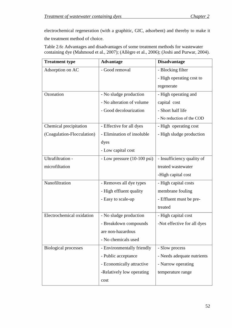
Treatment of wastewater containing dyes Chapter 2
52
electrochemical regeneration (with a graphitic, GIC, adsorbent) and thereby to make it
the treatment method of choice.
Table 2.6: Advantages and disadvantages of some treatment methods for wastewater containing dye (Mahmoud et al., 2007); (Allègre et al., 2006); (Joshi and Purwar, 2004).
Treatment type Advantage Disadvantage
Adsorption on AC - Good removal - Blocking filter
- High operating cost to
regenerate
Ozonation - No sludge production
- No alteration of volume
- Good decolourization
- High operating and
capital cost
- Short half life
- No reduction of the COD
Chemical precipitation
(Coagulation-Flocculation)
- Effective for all dyes
- Elimination of insoluble
dyes
- Low capital cost
- High operating cost
- High sludge production
Ultrafiltration -
microfiltation
- Low pressure (10-100 psi)
- Insufficiency quality of
treated wastewater
-High capital cost
Nanofiltration - Removes all dye types
- High effluent quality
- Easy to scale-up
- High capital costs
membrane fouling
- Effluent must be pre-
treated
Electrochemical oxidation - No sludge production
- Breakdown compounds
are non-hazardous
- No chemicals used
- High capital cost
-Not effective for all dyes
Biological processes - Environmentally friendly
- Public acceptance
- Economically attractive
-Relatively low operating
cost
- Slow process
- Needs adequate nutrients
- Narrow operating
temperature range

Batch adsorption and electrochemical regeneration Chapter 3
53
CHAPTER 3
BATCH ADSORPTION AND ELECTROCHEMICAL REGENERATION
In this Chapter, water treatment by batch adsorption with electrochemical regeneration
is evaluated. An experimental study is carried out using an organic dye as a model
contaminant in order to determine the effect of operating conditions on performance. In
addition the electrochemical regeneration of the GIC adsorbent has been evaluated and
the required charge for oxidation of an organic dye determined. Based on the data
obtained a design model is developed for water treatment by multi stage batch
adsorption with electrochemical regeneration.
3.1 Factors affecting physical adsorption
Many factors affect the amount of adsorption of a sorbate (solute) onto an adsorbent and
these include: surface area of adsorbent, nature of solute, nature of solvent, temperature,
pH and inorganic salts.
3.1.1 Surface area of adsorbent
The amount of adsorption increases with the surface area of adsorbent (e.g. due to a
decrease in the diameter of adsorbent particles) .
3.1.2 Nature of solute (adsorbate)
The adsorption of inorganic ions may vary greatly. Those which are strongly dissociated
such as sodium chloride essentially do not adsorb at all, whereas those which are only
weakly dissociated such as Mercuric Chloride adsorb well. The most important factor
appears to be the degree of ionization of the solute (Cooney, 1999).
For organic solutes, which are generally of greater interest and are the focus of this
study, a number of general statements may be made. The lower the aqueous solubility
usually the better the solute is adsorbed (Cooney, 1999). Also, the larger the molecule

Batch adsorption and electrochemical regeneration Chapter 3
54
the better it will adsorb, although there comes a point when the molecule becomes so
large that a significant number of the pores in porous adsorbents such as activated
carbon become inaccessible (Cooney, 1999). Amino groups, hydroxyl groups and
sulphonic acid groups generally reduce the degree of adsorption whereas the opposite is
true for nitro groups. Other substituent groups such as halogens and bond types can
have varying effects dependent upon other factors affecting the host molecule.
The molecular structure is also important with aromatic molecules adsorbing more
readily than aliphatic molecules of a similar size. Additionally, branched chain
molecules are more likely to be adsorbed than straight chain molecules of a similar
molecular weight (Cooney, 1999).
3.1.3 The nature of the solvent
Since the solvent competes with the adsorbent in attracting the solute (sorbate),
therefore its nature has an important effect. Thus, the amount of adsorption of an
organic solute out of an aqueous solution is less than its adsorption out of an organic
solvent (Cooney, 1999).
3.1.4 Temperature
Normally, increasing the temperature leads to a decrease in adsorption due to the
adsorbed molecules having greater energies and therefore becoming more likely to
release from the surface of the adsorbent (Cooney, 1999).
3.1.5 pH of the solution
The degree of adsorption is greatly influenced by the degree of ionization of the
adsorbate, which is in turn dependent on the pH of the solution (Cooney, 1999). When
the pH is such that the adsorbed species on the surface of the adsorbent all carry the
same electrical charge then the adsorbed species cannot pack together very densely on
the surface due to electrical repulsion. In contrast, when the adsorbate molecules are
neutral and carry no charge they can pack together more tightly on the adsorbent surface
and adsorption is maximised. Hence, it has been commonly observed that acidic species
adsorb at low pH and basic species at high pH (Cooney, 1999).

Batch adsorption and electrochemical regeneration Chapter 3
55
3.1.6 Effect of inorganic salts
The presence in the system of inorganic salts such as NaCl can enhance adsorption as
they can carry an opposite charge to the adsorbent and can fit into the spaces between
adsorbed molecules thereby screening the repulsive forces on the surface (Cooney,
1999).
3.2 Kinetics background
Adsorption processes are characterized by their kinetic and equilibrium behaviour. The
transport of the sorbate at the solid-solution interface (adsorbent) and the attachment of
the sorbate onto the adsorbent surface (i.e. the rate of the physio-chemical interaction at
the surface) determine the uptake rate of the sorbate and thus the kinetics of the process.
The degree of purification that may be achieved, the approximate amount of adsorbent
required to reach that degree of purification and the sensitivity of the process to the
concentration of the solute are predicted by the isotherms. Many mathematical models
have been studied in the literature in order to describe the kinetics of adsorption
processes. The Lagergren model (a pseudo first-order equation) and Ho model (a
pseudo second order equation) are widely used models for the adsorption kinetics of
organic compounds (Ho and McKay, 1998a); (Ho and McKay, 1999b).
A study of the kinetics of adsorption is desirable as it provides information about the
mechanism of adsorption, which is important for the efficiency of the process. In
addition, the design of an adsorption system for water treatment may be influenced or
even controlled by the adsorption kinetics. The rate of adsorption may be controlled by
mass transfer, intra-particle diffusion, or surface chemical kinetics. Several kinetic
models for the liquid phase have been widely used to describe experimental data. These
include pseudo first order, pseudo second order (Hamadi et al., 2001), intra-particle
diffusion (Weber and Morris, 1963), and mass transfer/intra-particle diffusion (Rengaraj
and Moon, 2002); (Findon et al., 1993) models.
The Lagergren model (Lagergren, 1898), a pseudo first-order model, is expressed as
follows:
)(1 tet qqk
dt
dq −= (3.1)

Batch adsorption and electrochemical regeneration Chapter 3
56
Where qt is the adsorbent loading at time t, and k1 is the first-order rate constant.
Integration of Equation (3.1) for a batch adsorption with qt = 0 at t = 0 gives:
)1( 1tket eqq −−= or tkqqq ete 1ln)ln( −=− (3.2)
The pseudo second-order model (Ho et al., 1996) is expressed as:
22 )( te
t qqkdt
dq−= (3.3)
where k2 is the second-order rate constant. Integration as before for a batch adsorption yields:
eet q
t
qkq
t +=2
2
1 or
tkq
tkqq
e
et
2
22
1+= (3.4)
The pseudo first and second order rate constants can be expressed as a function of
temperature by an Arrhenius type relationship (El-Khaiary, 2007) as follows:
−=RT
Ekk exp2,1 o
(3.5)
where k1,2 is the first or second order rate constant of sorption min−1 or g.mg−1.min−1,
respectively, ko is a temperature independent factor, (called the frequency factor) min−1
or g.mg−1.min−1, E is the activation energy of adsorption, J mol−1, R is the universal gas
constant, 8.314 J mol−1 K−1, and T is the solution absolute temperature, K.
The activation energy can be determined experimentally by measuring the rate constant
at a range of temperatures. Equation (3.5) can be rearranged to a linear form
−=TR
Ekk
1lnln 2,1 o
(3.6)
Thus a plot of ln(k1,2) versus 1/T may be used to determine the activation energy.
Previous studies of adsorption processes have suggested that physisorption processes
have relatively low activation energies in the range 5−40 kJ mol−1, while chemisorptions
processes have higher activation energies in the range 40−800 kJ mol−1 (Banerjee et al.,
1997).

Batch adsorption and electrochemical regeneration Chapter 3
57
3.3 Equilibrium isotherm
The equilibrium state is characterized by a concentration (loading) of adsorbate (solute)
in the solid phase (qe, mg g−1) which is in dynamic equilibrium with a solute
concentration in the liquid phase (Ce, mg L−1). A wide range values of qe versus Ce
values may be obtained by varying the amount of adsorbent (W, g), the initial
concentration of solute (Co, mg L−1), and the volume of liquid (Cooney, 1999). The
relationship between these qe and Ce can normally be fitted to one or more equilibrium
isotherm models.
3.3.1 Isotherm models
There are many models to describe the equilibrium behaviour for adsorption of
contaminants from water. However the three most widely used isotherm models are
Langmuir, Freundlich and Redlich-Peterson which are explained as follows (Vasanth
Kumar and Sivanesan, 2006):
3.3.1.1 Langmuir model
The Langmuir model (Equation (3.7)) was originally developed to describe and quantify
sorption on a set of distinct localized adsorption sites, and has been used to describe
both physical and chemical adsorption (Langmuir, 1916). This model is based upon the
following main assumptions (Dechow, 1989):
• Each active site interacts with only one sorbate molecule.
• Sorbate molecules are adsorbed on well defined localized sites and the saturation
coverage corresponds to complete occupancy of these sites.
• The adsorption sites are all energetically equivalent (homogeneous), and there is
no interaction between adjacent adsorbed molecules.
Based on these assumptions, the Langmuir relationship between qe and Ce is given by:
e
eLe bC
Cbkq
+=
1 (3.7)
where kL (mg g−1) and b (L mg−1) are the Langmuir constants related to the capacity of
adsorbent and energy of adsorption respectively.
This model is the most widely applied adsorption isotherm and has produced good
agreement with a variety of experimental data (Langmuir, 1918); (Zakaria et al., 2009).
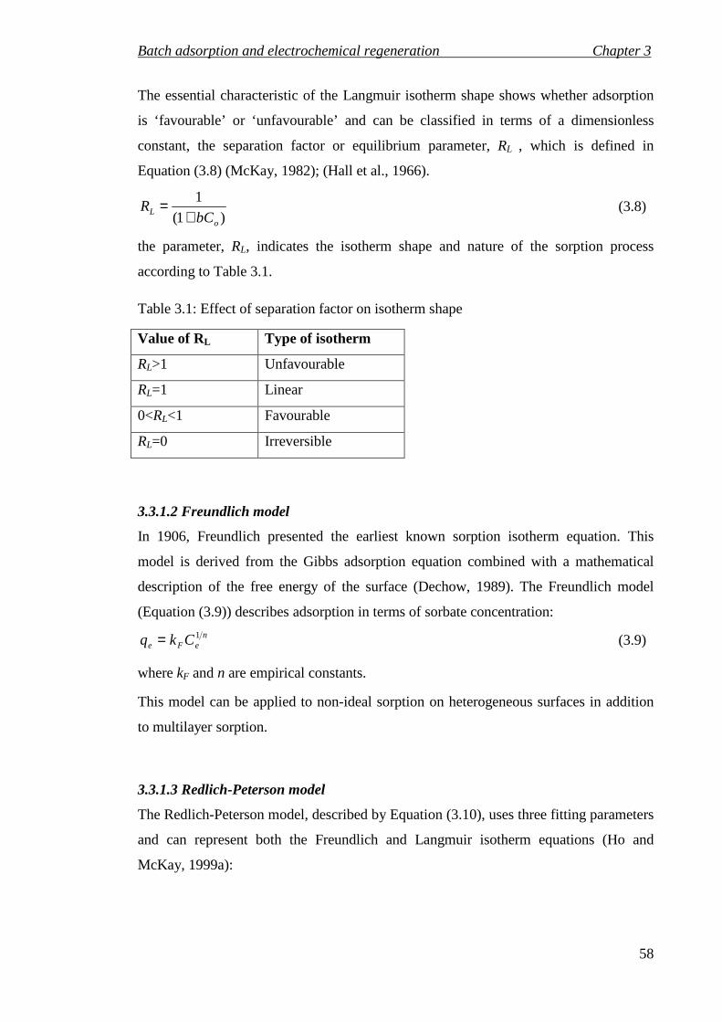
Batch adsorption and electrochemical regeneration Chapter 3
58
The essential characteristic of the Langmuir isotherm shape shows whether adsorption
is ‘favourable’ or ‘unfavourable’ and can be classified in terms of a dimensionless
constant, the separation factor or equilibrium parameter, RL , which is defined in
Equation (3.8) (McKay, 1982); (Hall et al., 1966).
)1(
1
oL bC
R+
= (3.8)
the parameter, RL, indicates the isotherm shape and nature of the sorption process
according to Table 3.1.
Table 3.1: Effect of separation factor on isotherm shape
Value of RL Type of isotherm
RL>1 Unfavourable
RL=1 Linear
0<RL<1 Favourable
RL=0 Irreversible
3.3.1.2 Freundlich model
In 1906, Freundlich presented the earliest known sorption isotherm equation. This
model is derived from the Gibbs adsorption equation combined with a mathematical
description of the free energy of the surface (Dechow, 1989). The Freundlich model
(Equation (3.9)) describes adsorption in terms of sorbate concentration:
neFe Ckq 1= (3.9)
where kF and n are empirical constants.
This model can be applied to non-ideal sorption on heterogeneous surfaces in addition
to multilayer sorption.
3.3.1.3 Redlich-Peterson model
The Redlich-Peterson model, described by Equation (3.10), uses three fitting parameters
and can represent both the Freundlich and Langmuir isotherm equations (Ho and
McKay, 1999a):
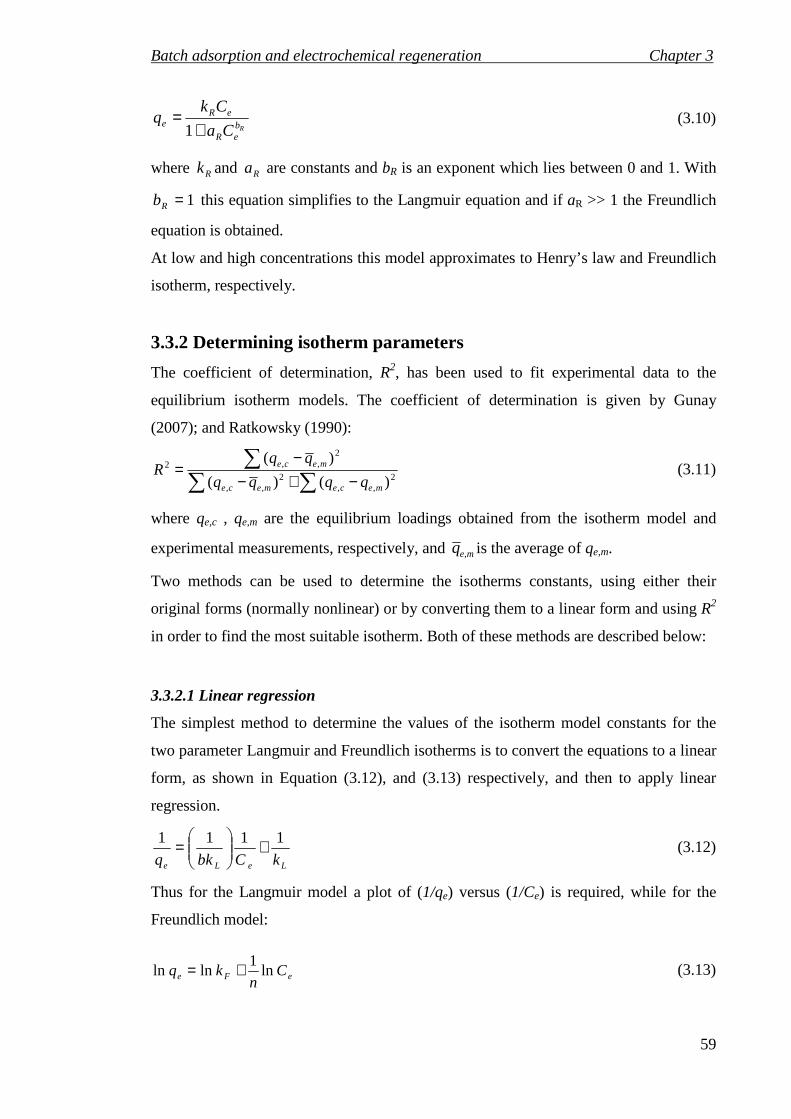
Batch adsorption and electrochemical regeneration Chapter 3
59
RbeR
eRe
Ca
Ckq
+=
1 (3.10)
where Rk and Ra are constants and bR is an exponent which lies between 0 and 1. With
1=Rb this equation simplifies to the Langmuir equation and if aR >> 1 the Freundlich
equation is obtained.
At low and high concentrations this model approximates to Henry’s law and Freundlich
isotherm, respectively.
3.3.2 Determining isotherm parameters
The coefficient of determination, R2, has been used to fit experimental data to the
equilibrium isotherm models. The coefficient of determination is given by Gunay
(2007); and Ratkowsky (1990):
∑ ∑∑
−+−−
=2
,,2
,,
2,,2
)()(
)(
mecemece
mece
qqqq
qqR (3.11)
where qe,c , qe,m are the equilibrium loadings obtained from the isotherm model and
experimental measurements, respectively, and meq , is the average of qe,m.
Two methods can be used to determine the isotherms constants, using either their
original forms (normally nonlinear) or by converting them to a linear form and using R2
in order to find the most suitable isotherm. Both of these methods are described below:
3.3.2.1 Linear regression
The simplest method to determine the values of the isotherm model constants for the
two parameter Langmuir and Freundlich isotherms is to convert the equations to a linear
form, as shown in Equation (3.12), and (3.13) respectively, and then to apply linear
regression.
LeLe kCbkq
1111 +
= (3.12)
Thus for the Langmuir model a plot of (1/qe) versus (1/Ce) is required, while for the
Freundlich model:
eFe Cn
kq ln1
lnln += (3.13)
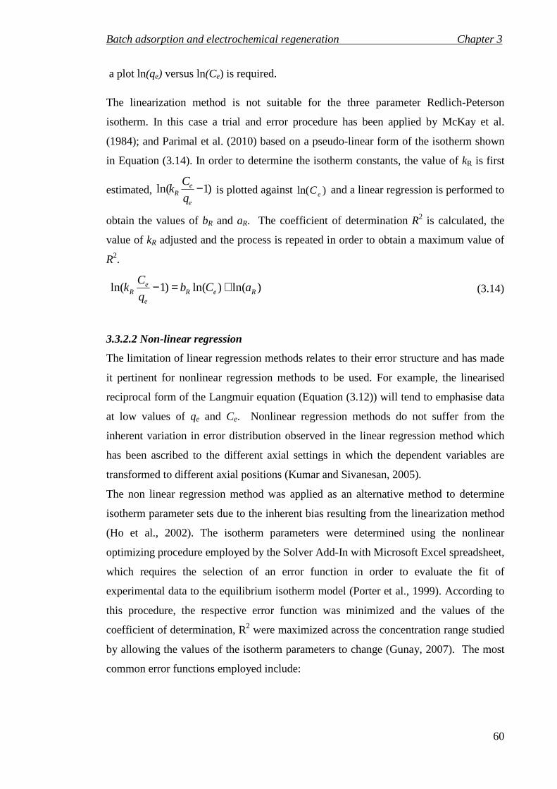
Batch adsorption and electrochemical regeneration Chapter 3
60
a plot ln(qe) versus ln(Ce) is required.
The linearization method is not suitable for the three parameter Redlich-Peterson
isotherm. In this case a trial and error procedure has been applied by McKay et al.
(1984); and Parimal et al. (2010) based on a pseudo-linear form of the isotherm shown
in Equation (3.14). In order to determine the isotherm constants, the value of kR is first
estimated, )1ln( −e
eR q
Ck is plotted against )ln( eC and a linear regression is performed to
obtain the values of bR and aR. The coefficient of determination R2 is calculated, the
value of kR adjusted and the process is repeated in order to obtain a maximum value of
R2.
)ln()ln()1ln( ReRe
eR aCb
q
Ck +=− (3.14)
3.3.2.2 Non-linear regression
The limitation of linear regression methods relates to their error structure and has made
it pertinent for nonlinear regression methods to be used. For example, the linearised
reciprocal form of the Langmuir equation (Equation (3.12)) will tend to emphasise data
at low values of qe and Ce. Nonlinear regression methods do not suffer from the
inherent variation in error distribution observed in the linear regression method which
has been ascribed to the different axial settings in which the dependent variables are
transformed to different axial positions (Kumar and Sivanesan, 2005).
The non linear regression method was applied as an alternative method to determine
isotherm parameter sets due to the inherent bias resulting from the linearization method
(Ho et al., 2002). The isotherm parameters were determined using the nonlinear
optimizing procedure employed by the Solver Add-In with Microsoft Excel spreadsheet,
which requires the selection of an error function in order to evaluate the fit of
experimental data to the equilibrium isotherm model (Porter et al., 1999). According to
this procedure, the respective error function was minimized and the values of the
coefficient of determination, R2 were maximized across the concentration range studied
by allowing the values of the isotherm parameters to change (Gunay, 2007). The most
common error functions employed include:
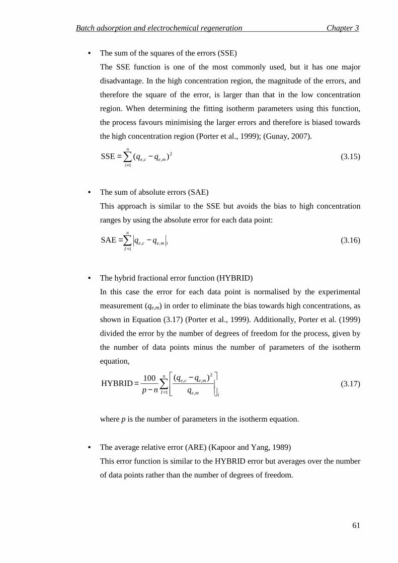
Batch adsorption and electrochemical regeneration Chapter 3
61
• The sum of the squares of the errors (SSE)
The SSE function is one of the most commonly used, but it has one major
disadvantage. In the high concentration region, the magnitude of the errors, and
therefore the square of the error, is larger than that in the low concentration
region. When determining the fitting isotherm parameters using this function,
the process favours minimising the larger errors and therefore is biased towards
the high concentration region (Porter et al., 1999); (Gunay, 2007).
∑=
−=n
imece qq
1
2,, )(SSE (3.15)
• The sum of absolute errors (SAE)
This approach is similar to the SSE but avoids the bias to high concentration
ranges by using the absolute error for each data point:
i
n
Imece qq∑
=
−=1
,,SAE (3.16)
• The hybrid fractional error function (HYBRID)
In this case the error for each data point is normalised by the experimental
measurement (qe,m) in order to eliminate the bias towards high concentrations, as
shown in Equation (3.17) (Porter et al., 1999). Additionally, Porter et al. (1999)
divided the error by the number of degrees of freedom for the process, given by
the number of data points minus the number of parameters of the isotherm
equation,
i
n
I me
mece
q
np ∑=
−−
=1 ,
2,, )(100
HYBRID (3.17)
where p is the number of parameters in the isotherm equation.
• The average relative error (ARE) (Kapoor and Yang, 1989)
This error function is similar to the HYBRID error but averages over the number
of data points rather than the number of degrees of freedom.

Batch adsorption and electrochemical regeneration Chapter 3
62
i
n
i me
mece
q
n ∑=−
=1 ,
,,100ARE (3.18)
• Marquardt’s Percent Standard Deviation (MPSD) (Marquardt, 1963)
The MPSD again as a similar form but using a root mean squared approach
∑=
−−
=n
i ime
ceme
q
np 1
2
,
,,1.100MPSD (3.19)

Batch adsorption and electrochemical regeneration Chapter 3
63
3.4 Characterisation of electrochemical regeneration performance Electrochemical regeneration of an adsorbent is normally characterised by its efficiency
and the performance of the adsorption / regeneration process. The theoretical charge
(TC) required for decomposition or mineralisation of pollutant materials in the
electrochemical cell was estimated from (Brown and Roberts, 2007); (Comninellis and
Pulgarin, 1991):
w
eo
M
VFCC )(nTC
−= (3.20)
where n is the number of electrons required per molecule of pollutant oxidised, F is
Faraday’s constant (96487 C mol−1), V is the solution volume (L), and Mw is the
molecular weight of the pollutant molecule.
The current efficiency, η, is equal to theoretical charge (TC) divided by actual charge
passed as follow:
ItM
VFCCn
w
eo )( −=η (3.21)
where I is the DC current supplied (A), and t is the electrochemical regeneration time.
The regeneration efficiency, rη , for adsorption and electrochemical regeneration was
calculated from Equation (3.22) (Narbaitz and Karimi-Jashni, 2009):
%100.i
rr q
q=η (3.22)
where qi is the adsorption capacity of fresh adsorbent, and qr is the adsorption capacity
of adsorbent after regeneration (mg g−1).

Batch adsorption and electrochemical regeneration Chapter 3
64
3.5 Materials and experimental methodologies
The experimental methodologies for the batch mode are divided into three parts;
adsorption (removal of AV17 from solution), electrochemical regeneration of adsorbent
(Nyex®1000), and multi-stage adsorption and electrochemical regeneration.
3.5.1 Adsorption methodology
3.5.1.1 Materials Sorbate
There are a wide range of organic dyes used in industry. This study focuses on Acid
Violet 17 (AV17, Figure 3.1), which is a powdered anionic tri-phenyl methane (TPM)
dye which dissolves readily in hot water, chemical formula C41H44N3NaO6S2 and
formula weight 761.9. TPM dyes are a large class of synthetic dyes that are widely used
in the textiles industry and are also used to stain bacteria and tissue cultures
(Venkataraman, 1952). Commercial dyes are typically prepared as a mixture of the dye
compound and an inorganic salt. A powdered form of AV17, supplied by KEMTEX
Educational Supplies Ltd under the trade name Kenanthrol Violet 2B, was used in this
study. Total organic carbon (TOC) analysis of samples of the dye dissolved in deionised
water indicated that the concentration of the AV17 in the dye as supplied was 22 wt%,
the remainder being an inorganic salt.

Batch adsorption and electrochemical regeneration Chapter 3
65
CH 3
CH 3 N
N+
CH 3
S OO
O-
S
O
O
O-
N
CH 3
N a+
Figure 3.1: Chemical structure of Acid Violet 17.
Sorbent
Figure 3.2 shows a scanning electron microscope (SEM) image of Nyex®1000
(bisulphate intercalated GIC) as supplied by Arvia® Technology Ltd. The Nyex®
particles have a characteristic flake like shape associated with the graphite precursor.
The specification for Nyex®1000 provided by Arvia® Technology Ltd indicates a
carbon content of ~95 wt%, a typical particle diameter of ~360–500 µm (consistent with
Figure 3.2), with particle diameters ranging between 100 and 700 µm in size. The
Brunauer Emmett Teller (BET) surface area of Nyex®1000 determined by nitrogen
adsorption was found to be 1.0 m2 g−1, which is very small compared to activated
carbon which may have a surface area up to 2000 m2 g−1 (Streat et al., 1995). However,
as discussed in section 2.2.1.2 (Chapter 2), the Nyex®1000 can be rapidly regenerated
so that its surface area can be reused intensively.
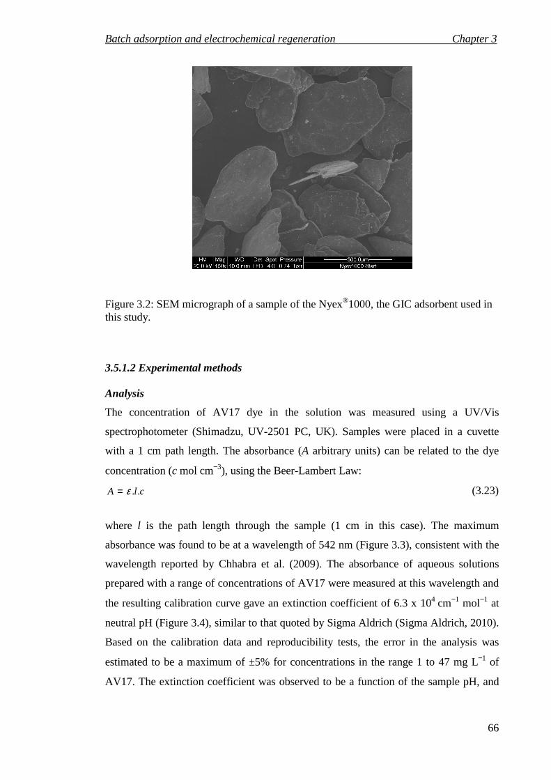
Batch adsorption and electrochemical regeneration Chapter 3
66
Figure 3.2: SEM micrograph of a sample of the Nyex®1000, the GIC adsorbent used in this study.
3.5.1.2 Experimental methods Analysis
The concentration of AV17 dye in the solution was measured using a UV/Vis
spectrophotometer (Shimadzu, UV-2501 PC, UK). Samples were placed in a cuvette
with a 1 cm path length. The absorbance (A arbitrary units) can be related to the dye
concentration (c mol cm−3), using the Beer-Lambert Law:
clA ..ε= (3.23)
where l is the path length through the sample (1 cm in this case). The maximum
absorbance was found to be at a wavelength of 542 nm (Figure 3.3), consistent with the
wavelength reported by Chhabra et al. (2009). The absorbance of aqueous solutions
prepared with a range of concentrations of AV17 were measured at this wavelength and
the resulting calibration curve gave an extinction coefficient of 6.3 x 104 cm−1 mol−1 at
neutral pH (Figure 3.4), similar to that quoted by Sigma Aldrich (Sigma Aldrich, 2010).
Based on the calibration data and reproducibility tests, the error in the analysis was
estimated to be a maximum of ±5% for concentrations in the range 1 to 47 mg L−1 of
AV17. The extinction coefficient was observed to be a function of the sample pH, and

Batch adsorption and electrochemical regeneration Chapter 3
67
calibration curves were prepared for a range of pH condition (see Appendix A, Figure
A.1).
Figure 3.3: UV-Visible Spectra Acid Violet 17 at 22 mg L−1.
Figure 3.4: Calibration curve of Acid Violet 17.
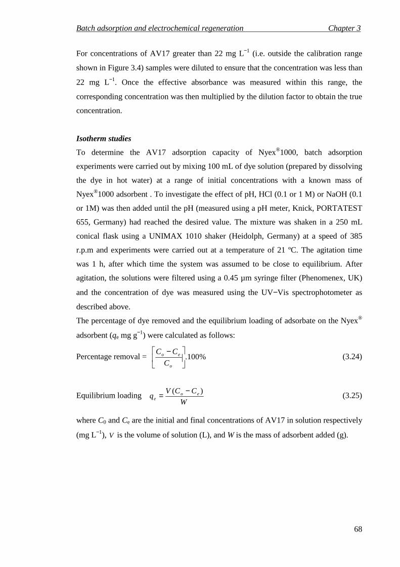
Batch adsorption and electrochemical regeneration Chapter 3
68
For concentrations of AV17 greater than 22 mg L−1 (i.e. outside the calibration range
shown in Figure 3.4) samples were diluted to ensure that the concentration was less than
22 mg L−1. Once the effective absorbance was measured within this range, the
corresponding concentration was then multiplied by the dilution factor to obtain the true
concentration.
Isotherm studies
To determine the AV17 adsorption capacity of Nyex®1000, batch adsorption
experiments were carried out by mixing 100 mL of dye solution (prepared by dissolving
the dye in hot water) at a range of initial concentrations with a known mass of
Nyex®1000 adsorbent . To investigate the effect of pH, HCl (0.1 or 1 M) or NaOH (0.1
or 1M) was then added until the pH (measured using a pH meter, Knick, PORTATEST
655, Germany) had reached the desired value. The mixture was shaken in a 250 mL
conical flask using a UNIMAX 1010 shaker (Heidolph, Germany) at a speed of 385
r.p.m and experiments were carried out at a temperature of 21 ºC. The agitation time
was 1 h, after which time the system was assumed to be close to equilibrium. After
agitation, the solutions were filtered using a 0.45 µm syringe filter (Phenomenex, UK)
and the concentration of dye was measured using the UV−Vis spectrophotometer as
described above.
The percentage of dye removed and the equilibrium loading of adsorbate on the Nyex®
adsorbent (qe mg g−1) were calculated as follows:
Percentage removal = %100.
−
o
eo
C
CC (3.24)
Equilibrium loading W
CCVq eo
e
)( −= (3.25)
where C0 and Ce are the initial and final concentrations of AV17 in solution respectively
(mg L−1), V is the volume of solution (L), and W is the mass of adsorbent added (g).
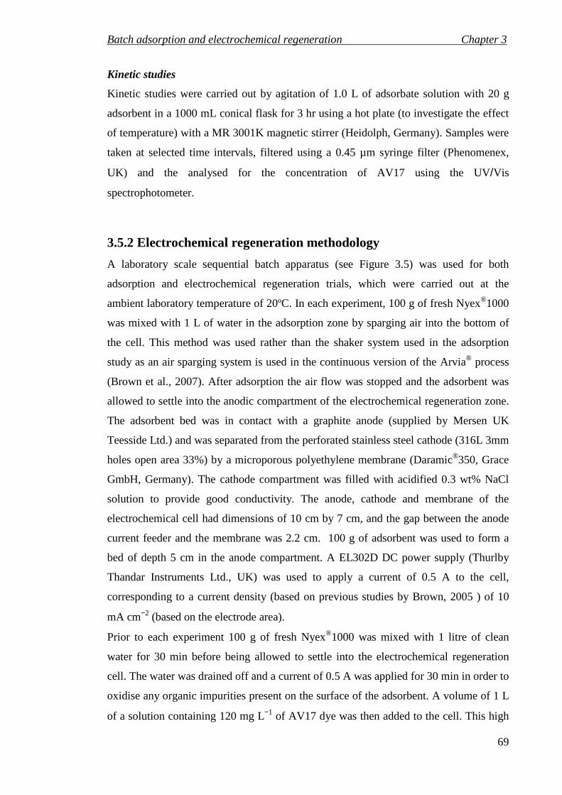
Batch adsorption and electrochemical regeneration Chapter 3
69
Kinetic studies
Kinetic studies were carried out by agitation of 1.0 L of adsorbate solution with 20 g
adsorbent in a 1000 mL conical flask for 3 hr using a hot plate (to investigate the effect
of temperature) with a MR 3001K magnetic stirrer (Heidolph, Germany). Samples were
taken at selected time intervals, filtered using a 0.45 µm syringe filter (Phenomenex,
UK) and the analysed for the concentration of AV17 using the UV/Vis
spectrophotometer.
3.5.2 Electrochemical regeneration methodology
A laboratory scale sequential batch apparatus (see Figure 3.5) was used for both
adsorption and electrochemical regeneration trials, which were carried out at the
ambient laboratory temperature of 20ºC. In each experiment, 100 g of fresh Nyex®1000
was mixed with 1 L of water in the adsorption zone by sparging air into the bottom of
the cell. This method was used rather than the shaker system used in the adsorption
study as an air sparging system is used in the continuous version of the Arvia® process
(Brown et al., 2007). After adsorption the air flow was stopped and the adsorbent was
allowed to settle into the anodic compartment of the electrochemical regeneration zone.
The adsorbent bed was in contact with a graphite anode (supplied by Mersen UK
Teesside Ltd.) and was separated from the perforated stainless steel cathode (316L 3mm
holes open area 33%) by a microporous polyethylene membrane (Daramic®350, Grace
GmbH, Germany). The cathode compartment was filled with acidified 0.3 wt% NaCl
solution to provide good conductivity. The anode, cathode and membrane of the
electrochemical cell had dimensions of 10 cm by 7 cm, and the gap between the anode
current feeder and the membrane was 2.2 cm. 100 g of adsorbent was used to form a
bed of depth 5 cm in the anode compartment. A EL302D DC power supply (Thurlby
Thandar Instruments Ltd., UK) was used to apply a current of 0.5 A to the cell,
corresponding to a current density (based on previous studies by Brown, 2005 ) of 10
mA cm−2 (based on the electrode area).
Prior to each experiment 100 g of fresh Nyex®1000 was mixed with 1 litre of clean
water for 30 min before being allowed to settle into the electrochemical regeneration
cell. The water was drained off and a current of 0.5 A was applied for 30 min in order to
oxidise any organic impurities present on the surface of the adsorbent. A volume of 1 L
of a solution containing 120 mg L−1 of AV17 dye was then added to the cell. This high
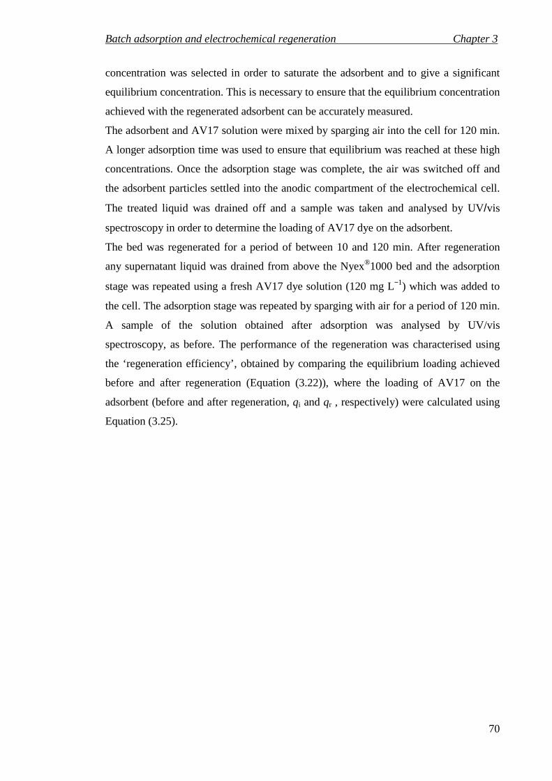
Batch adsorption and electrochemical regeneration Chapter 3
70
concentration was selected in order to saturate the adsorbent and to give a significant
equilibrium concentration. This is necessary to ensure that the equilibrium concentration
achieved with the regenerated adsorbent can be accurately measured.
The adsorbent and AV17 solution were mixed by sparging air into the cell for 120 min.
A longer adsorption time was used to ensure that equilibrium was reached at these high
concentrations. Once the adsorption stage was complete, the air was switched off and
the adsorbent particles settled into the anodic compartment of the electrochemical cell.
The treated liquid was drained off and a sample was taken and analysed by UV/vis
spectroscopy in order to determine the loading of AV17 dye on the adsorbent.
The bed was regenerated for a period of between 10 and 120 min. After regeneration
any supernatant liquid was drained from above the Nyex®1000 bed and the adsorption
stage was repeated using a fresh AV17 dye solution (120 mg L−1) which was added to
the cell. The adsorption stage was repeated by sparging with air for a period of 120 min.
A sample of the solution obtained after adsorption was analysed by UV/vis
spectroscopy, as before. The performance of the regeneration was characterised using
the ‘regeneration efficiency’, obtained by comparing the equilibrium loading achieved
before and after regeneration (Equation (3.22)), where the loading of AV17 on the
adsorbent (before and after regeneration, qi and qr , respectively) were calculated using
Equation (3.25).
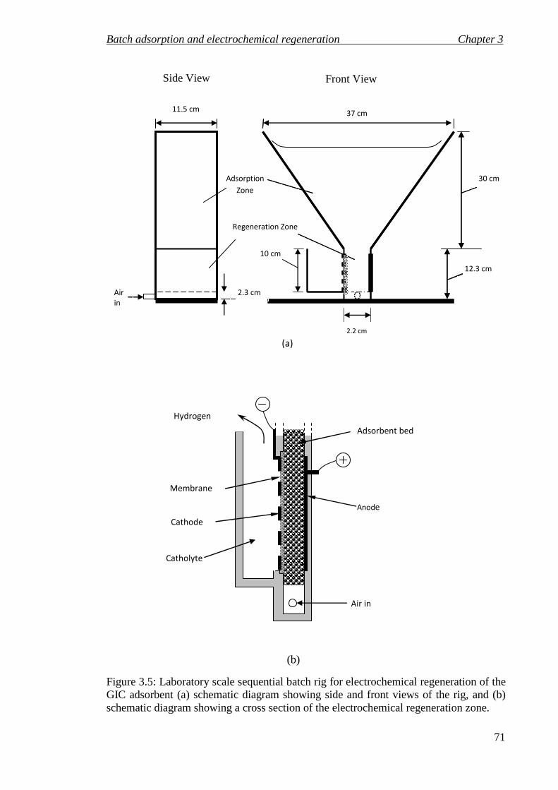
Batch adsorption and electrochemical regeneration Chapter 3
71
Regeneration Zone
Catholyte
Adsorbent bed
Anode
Membrane
Cathode
Hydrogen
Air in
(b)
(a)
Front View Side View
Adsorption
Zone
10 cm
37 cm
30 cm
12.3 cm
2.2 cm
11.5 cm
Air
in
2.3 cm
Figure 3.5: Laboratory scale sequential batch rig for electrochemical regeneration of the GIC adsorbent (a) schematic diagram showing side and front views of the rig, and (b) schematic diagram showing a cross section of the electrochemical regeneration zone.

Batch adsorption and electrochemical regeneration Chapter 3
72
3.5.3 Multi-stage batch process methodology
A similar technique was used for multi-stage batch adsorption and electrochemical
regeneration, but in this case the solution was not drained off after the adsorption cycle.
The initial concentration of AV17 dye was much higher, 668 mg L−1 as this solution
was treated by a series of adsorption/regeneration cycles. In order to achieve significant
treatment on each cycle, the amount of Nyex®1000 used was increased to 125 g, which
formed a bed of 7 cm depth in the anode compartment. In addition, the adsorption time
was reduced to 60 minutes and the regeneration time was 30 min.

Batch adsorption and electrochemical regeneration Chapter 3
73
3.6 Experimental results and discussion
3.6.1 Adsorption kinetics
3.6.1.1 Effect of initial concentration The kinetics of AV17 sorption on Nyex®1000 was studied at room temperature (23 ºC)
using batch experiments with dye concentrations in the range 13 to 26 mg L−1 and an
adsorbent dose of 20 g L−1. Figure 3.6 shows the decrease in the concentration of AV17
following addition of the adsorbent. As the initial AV17 dye concentration was
increased from 13 to 26 mg L−1, the percentage removal at equilibrium decreased from
96.3% to 67.3% whilst the adsorbate loading on the solid phase increased from 0.64 to
0.88 mg g−1 (see Figure 3.7). It is also evident from Figure 3.6 that most of the dye was
adsorbed during the first 30 min after addition of the adsorbent. This is due to high
driving force for the transfer of dye from solution to the surface of Nyex®1000 at the
start of adsorption, and the rapid mass transfer to the surface of the adsorbent. The
adsorption can be considered to be rapid when compared to porous activated carbon
adsorbents, which can take several days to reach equilibrium (Peel and Benedek, 1980).
The adsorption appears to occur in a series of waves, possibly corresponding to
different types of adsorption sites on the surface or multilayer adsorption. Equilibrium
was achieved after around 60 min, although a very gradual decrease in concentration
was observed at long times.

Batch adsorption and electrochemical regeneration Chapter 3
74
Figure 3.6: Variation in the concentration of AV17 during batch adsorption on Nyex®1000 at 23 °C with an adsorbent dosage of 20 g L−1 for a range of initial concentration.
In order to fit kinetic models to the adsorption data, the variation of adsorbent loading
(qt) with time was determined for the data plotted in Figure 3.6. The pseudo first order
(Equation 3.2) and pseudo second order (Equation 3.4) models were then fitted to the
data using a least squared error method. Each model was fitted to the four sets of data
together, using a single value for the rate constant and different values for equilibrium
loading for each initial concentration. Thus five parameters (four equilibrium loadings
and the rate constant) were adjusted to obtain the least squared error for each model.
The Solver Add-In in Microsoft Excel® was used to minimise the sum of absolute error
(SAE, Equation 3.16) between the model and the data in each case. Neither of the
models gave a very good fit to the data, but the error obtained using the pseudo second-
order model was less than half that obtained with the pseudo first-order model. Figure
3.7 shows the variation of loading with time and the curve obtained from the pseudo
second-order model fitted to the data. The values of fitted rate constants and
equilibrium loadings obtained from the kinetic models are shown in Table 3.2. The
values of equilibrium loading obtained in the experiments (qe,m) are closer to the values
obtained with the pseudo second-order model than those from the pseudo first-order
model.

Batch adsorption and electrochemical regeneration Chapter 3
75
Table 3.2: Kinetic rate constants for the adsorption of AV17 onto Nyex®1000 dose 20 g L−1, where qe1 and qe2 are the fitted equilibrium loadings for the first order and second order models respectively.
C0 mg L−−−−1
qe,m mg g−−−−1
k1 min−−−−1
qe1 mg g−−−−1
k2 g mg−−−−1 min−−−−1
qe2 mg g−−−−1
13 0.64 0.176 0.61 0.41 0.65
18 0.80 0.76 0.80
23 0.81 0.76 0.81
26 0.88 0.81 0.856
Figure 3.7: Variation in the adsorbent loading of AV17 during batch adsorption on Nyex®1000 calculated from data in Figure 3.6. The lines show the pseudo second order kinetic model (Equation 3.4) fitted to the data.

Batch adsorption and electrochemical regeneration Chapter 3
76
3.6.1.2 Effect of temperature
The adsorption of AV17 dye onto Nyex®1000 was studied using batch adsorption tests
at a range of temperatures between 30 and 70°C. Figure 3.8 shows the results obtained,
including the curves obtained from fitting the pseudo second-order model to each set of
data. The parameters obtained from the fitted pseudo second-order model are shown in
Table 3.3. These results show that the equilibrium loading increased with increasing
temperature. Previous studies of adsorption of dyes on activated carbon have shown
similar increases in equilibrium loading with temperature (Demirbas et al., 2008);
(Thinakaran et al., 2008). This has been attributed to an increase in the mobility of the
large dye ion with temperature, and this is likely to be the cause of the increase
observed in this study.
The second order rate constant was observed to increase slightly with temperature as
shown in Table 3.3. The Arrhenius plot (Figure 3.9) for the data shown in Table 3.3
indicate that the activation energy for the adsorption of AV17 onto Nyex®1000 is
around 4.2 kJ mol−1, although there is clearly significant uncertainty in this value.
Previous studies have suggested that physisorption processes have low activation
energy, in the range 5 to 40 kJ mol−1, while for chemisorptions processes the activation
energy is higher, typically 40 to 800 kJ mol−1 (Banerjee et al., 1997). Although there is
significant uncertainty in the value of the activation energy obtained, it is an order of
magnitude lower than that expected for a chemisorption process.
Table 3.3: Parameters obtained for the pseudo second-order model fitted to the adsorption data plotted in Figure 3.8 at a range of temperature and 22 mg L−1 initial dye concentration of AV17.
T
oC
qe,m
mg g−−−−1
k2
g mg−−−−1 min−−−−1
qe2
mg g−−−−1
30 0.855 0.430 0.810
40 0.894 0.440 0.824
57 0.910 0.493 0.844
66 0.920 0.500 0.865
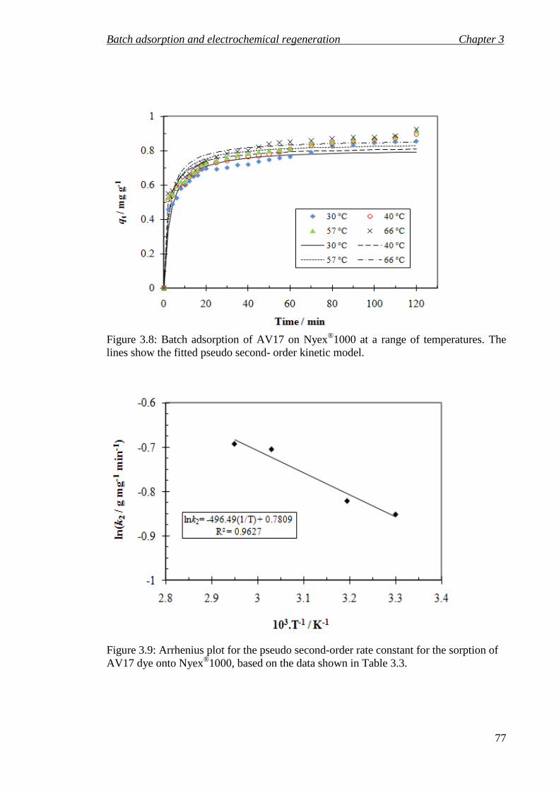
Batch adsorption and electrochemical regeneration Chapter 3
77
Figure 3.8: Batch adsorption of AV17 on Nyex®1000 at a range of temperatures. The lines show the fitted pseudo second- order kinetic model.
Figure 3.9: Arrhenius plot for the pseudo second-order rate constant for the sorption of AV17 dye onto Nyex®1000, based on the data shown in Table 3.3.
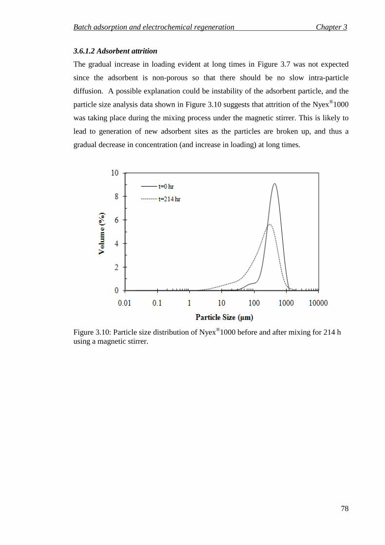
Batch adsorption and electrochemical regeneration Chapter 3
78
3.6.1.2 Adsorbent attrition
The gradual increase in loading evident at long times in Figure 3.7 was not expected
since the adsorbent is non-porous so that there should be no slow intra-particle
diffusion. A possible explanation could be instability of the adsorbent particle, and the
particle size analysis data shown in Figure 3.10 suggests that attrition of the Nyex®1000
was taking place during the mixing process under the magnetic stirrer. This is likely to
lead to generation of new adsorbent sites as the particles are broken up, and thus a
gradual decrease in concentration (and increase in loading) at long times.
Figure 3.10: Particle size distribution of Nyex®1000 before and after mixing for 214 h using a magnetic stirrer.

Batch adsorption and electrochemical regeneration Chapter 3
79
3.6.2 Adsorption isotherm
3.6.2.1 Equilibrium isotherm
Based on the kinetic data shown in Figures 3.6 and 3.7, it was assumed that equilibrium
was achieved during the batch studies after around 60 min. The equilibrium behaviour
of the sorption of AV17 onto Nyex®1000 was thus studied in a batch process by mixing
2 g of sorbent with 100 mL of dye solution at a range of concentrations (4.8–46 mg L−1)
for 60 min. Assuming that equilibrium was achieved, Figure 3.11 shows the adsorption
isotherm obtained at room temperature. The data was fitted to the Langmuir, Freundlich
and Redlich-Peterson equations (Langmuir, 1916); (Dechow, 1989); (Ho and McKay,
1999a) by finding the parameter values which gave a maximum value of the correlation
coefficient between the data (qe and Ce) and the model in each case. It is clear from
Figure 3.11 and the values of the correlation coefficient R2 shown in Table 3.4 that the
Langmuir and Redlich-Peterson models (which are almost indistinguishable) give a
much better fit to the data than the Freundlich model. The fitted parameter values for the
three models are shown in Table 3.4. The value of bR fitted for the Redlich-Peterson
model is one, which is consistent with the close agreement with the fitted Langmuir
model plotted in Figure 3.11. As expected, the maximum loading achieved is around
two orders of magnitude less than that which can be achieved with activated carbon
(e.g. Namasivayam et al., 2007; and Walker and Weatherley, 2001).
Table 3.4: Langmuir, Freundlich and Redlich-Peterson isotherm constants for sorption of Acid Violet 17 onto Nyex®1000, dosage 2 g/100 mL.
Isotherm
model
kL
mg g−−−−1
b
L mg−−−−1
kF
mg(1-1/n ) L1/n
g−−−−1
1/n kR
L g−−−−1
aR
LbR mg-bR
bR R2
Langmuir 0.987 0.31 0.968
Freundlich 0.34 0.30 0.855
Redlich-
Peterson
0.305 0.31 1.0 0.967

Batch adsorption and electrochemical regeneration Chapter 3
80
Figure 3.11: Isotherm for the sorption of AV17 onto Nyex®1000 at room temperature, where Ce was determined after mixing 100 mL of solution with 2 g of Nyex for 60 min.
There is little data available in the literature on the adsorption of AV17 by activated
carbon, but there is some data on other dyes such as methylene blue (El Qada et al.,
2008). The comparison of Langmuir isotherm constants for adsorption of organic dye
calculated in this work with those determined by El Qada et al. (2008) for activated
carbon produced by steam activation are shown in Table 3.5. The low surface area of
the Nyex®1000 means that it is a low capacity adsorbent material. However, if the
adsorptive capacity (kL) is normalised with the specific surface area, it is found that the
Nyex® adsorbent is able adsorb a higher mass of dye per unit area than the activated
carbons studied (albeit for a different adsorbate). This suggests that either the Nyex®
has more adsorption sites per unit area or (more likely) that some of the activated
carbon surface area in the micropores is not accessible to the dye molecules.
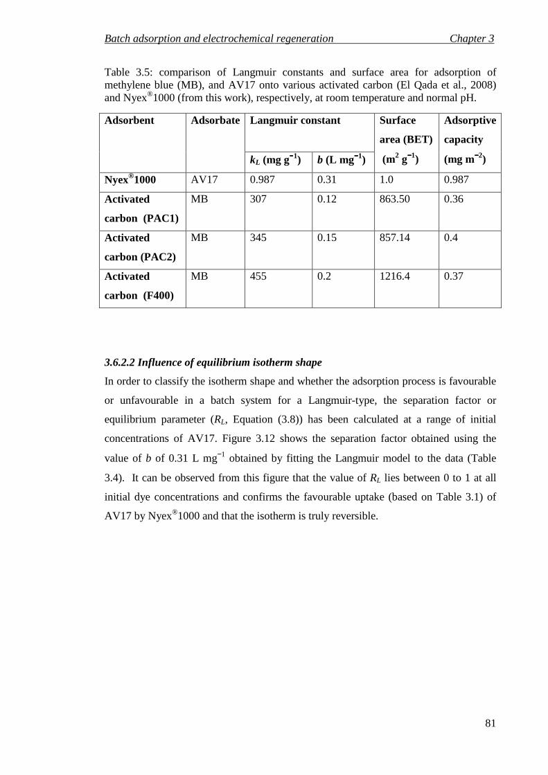
Batch adsorption and electrochemical regeneration Chapter 3
81
Table 3.5: comparison of Langmuir constants and surface area for adsorption of methylene blue (MB), and AV17 onto various activated carbon (El Qada et al., 2008) and Nyex®1000 (from this work), respectively, at room temperature and normal pH.
Adsorbent Adsorbate Langmuir constant
Surface
area (BET)
(m2 g−−−−1)
Adsorptive
capacity
(mg m−−−−2) kL (mg g−−−−1) b (L mg−−−−1)
Nyex®1000 AV17 0.987 0.31 1.0 0.987
Activated
carbon (PAC1)
MB 307 0.12 863.50 0.36
Activated
carbon (PAC2)
MB 345 0.15 857.14 0.4
Activated
carbon (F400)
MB 455 0.2 1216.4 0.37
3.6.2.2 Influence of equilibrium isotherm shape
In order to classify the isotherm shape and whether the adsorption process is favourable
or unfavourable in a batch system for a Langmuir-type, the separation factor or
equilibrium parameter (RL, Equation (3.8)) has been calculated at a range of initial
concentrations of AV17. Figure 3.12 shows the separation factor obtained using the
value of b of 0.31 L mg−1 obtained by fitting the Langmuir model to the data (Table
3.4). It can be observed from this figure that the value of RL lies between 0 to 1 at all
initial dye concentrations and confirms the favourable uptake (based on Table 3.1) of
AV17 by Nyex®1000 and that the isotherm is truly reversible.

Batch adsorption and electrochemical regeneration Chapter 3
82
Figure 3.12: Separation factor for Acid Violet 17 dye onto Nyex®1000 at 23 °C.
The Langmuir model also describes the equilibrium between the highest fluid
concentration, Co, and solid phase concentration, qo (Equation 3.26) in equilibrium with
Co.
o
oLo bC
Cbkq
+=
1 (3.26)
The general Langmuir relation (Equation 3.7) can be derived from Equation (3.26):
e
o
o
e
o
e
bC
bC
C
C
q
q
++=
1
1 (3.27)
Defining a dimensionless solid phase concentration as oe qqq = , and a dimensionless
liquid phase concentration as oe CCC = , (each of these terms is bounded by the values
0 and 1) we obtain:
CRR
Cq
LL )1( −+= (3.28)
The experimental data from Figure 3.11 are plotted in dimensionless form in Figure
3.13, along with the theoretical form (Equation 3.28) for a range of values of the
separation factor The experimental data was fitted to Equation (3.28) by finding the
value of RL that gave a minimum in the sum of the absolute error (SAE) between the (q,

Batch adsorption and electrochemical regeneration Chapter 3
83
C) data and the Equation (3.28).This minimum was obtained numerically using the
Solver tool in Microsoft Excel. It is clear from Figure 3.13 that the experimental data of
the AV17 dye isotherm indicated a value of RL = 0.06, which suggests that the
adsorption process is favourable according to Table 3.1, i.e. 0<RL<1. Similar results
have been recorded for separation factors for the adsorption of the dye AV17 by onto
activated carbon prepared from sunflower seed hull (Thinakaran et al., 2008) and orange
peel (Sivaraj et al., 2001)
Figure 3.13: Isotherm shape for adsorption of AV17 onto Nyex®1000 as function of separation factor.
3.6.2.3 Influence of pH
The effect of pH on the adsorption of AV17 onto Nyex®1000 was studied by varying
the initial pH of the dye solution from 2 to 11 using 0.1 or 1 M HCl or 0.1 or 1 M
NaOH. For an initial concentration of AV17 of 22 mg L−1, the percentage of AV17
removed and the loading at equilibrium (i.e. after 60 min) is plotted in Figure 3.14. It
can be seen from this figure that at low pH (pH < 4) the percentage removal and the
equilibrium loading increased with decreasing pH, corresponding to a lower equilibrium
concentration and a higher loading of AV17 on the adsorbent. The increased loading is
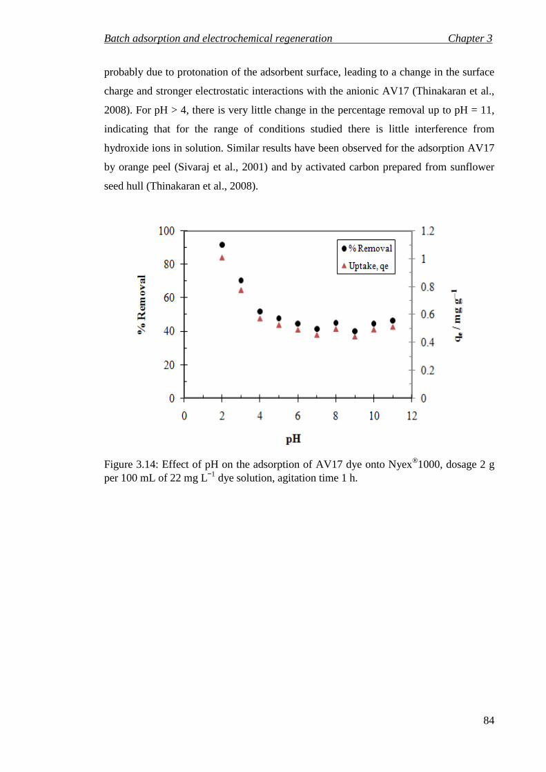
Batch adsorption and electrochemical regeneration Chapter 3
84
probably due to protonation of the adsorbent surface, leading to a change in the surface
charge and stronger electrostatic interactions with the anionic AV17 (Thinakaran et al.,
2008). For pH > 4, there is very little change in the percentage removal up to pH = 11,
indicating that for the range of conditions studied there is little interference from
hydroxide ions in solution. Similar results have been observed for the adsorption AV17
by orange peel (Sivaraj et al., 2001) and by activated carbon prepared from sunflower
seed hull (Thinakaran et al., 2008).
Figure 3.14: Effect of pH on the adsorption of AV17 dye onto Nyex®1000, dosage 2 g per 100 mL of 22 mg L−1 dye solution, agitation time 1 h.

Batch adsorption and electrochemical regeneration Chapter 3
85
3.6.3 Electrochemical regeneration
The liquid phase concentration of AV17 dye after adsorption was found to be in the
range 13.2 to 15.4 mg L−1, corresponding to a loading of AV17 on the Nyex®1000
adsorbent of 1.07 to 1.05 mg g−1. This was slightly higher than the maximum value of kL
(0.987 mg g−1) predicted from the Langmuir adsorption isotherm (Table 3.4), possibly
due to attrition or surface modification of the adsorbent during the washing procedure.
It was found that the full adsorption capacity was recovered after 40 min of
electrochemical regeneration, corresponding to a charge passed of 12 C g−1 (Figure
3.15). Further increase in the regeneration time led to an increase in the adsorption
capacity to a value around 10 % higher than the original capacity. There are a number of
possible reasons for this increase in adsorption capacity after regeneration. Previous
studies (Brown, 2005) have suggested that the electrochemical regeneration can lead to
a slight roughening of the adsorbent surface, and thus an increase in the specific surface
area available for adsorption.
For regeneration times less than 40 min, the full capacity of the adsorbent was not
recovered. This suggests that some AV17 or its breakdown products remained adsorbed
on the surface of the GIC adsorbent. When the full adsorption capacity was recovered,
the AV17 dye had either been fully mineralised, or breakdown products were formed
which were not adsorbed on the adsorbent and were thus released into the water.
Chemical oxygen demand (COD) analysis of treated water (unpublished data from
Arvia Technology Ltd) have not found organic breakdown products in solution,
suggesting that breakdown products remain adsorbed until full mineralisation is
achieved.
It is possible to estimate the charge required to fully mineralise the dye, however this
will depend on the products formed. The maximum charge required can be estimated by
assuming complete anodic oxidation of the AV17 to carbon dioxide, sulphate and
nitrate:
−−−++ +++++→+ 224e3NO2SONa230H41COO93HSNaONHC 324222634441 (3.29)
Alternatively a lower estimate of the charge required for mineralisation can be obtained
by assuming that the products were carbon monoxide, sulphide and nitrogen:
−−++ +++++→+ 111e1.5N2SNa114H41COO35HSNaONHC 22
22634441 (3.30)
It is possible that neither of these equations represents the true situation, which may be
far more complex than these simple stoichiometries suggest. There may be complex but

Batch adsorption and electrochemical regeneration Chapter 3
86
uncoloured breakdown product formation that is not described by these equations.
However for the purposes of the model Equation (3.30) has been selected as it is a good
fit to the data. As discussed in Section 3.4, the theoretical charge for mineralisation of
the AV17 dye can be estimated from:
Theoretical charge = w
e
M
nFq (3.31)
where n is the number of electrons required per molecule of dye oxidised, F is
Faraday’s constant (96487 C mol−1), and Mw is the molecular weight of the dye (761.9 g
mol−1). The value of qe obtained was 1.06 mg g−1, and using n = 111 and 224 [based on
Equations (3.29) and (3.30) respectively] the theoretical charge required for
mineralisation of the AV17 would be between 15 and 30 C g−1. Comparison of these
values with the data in Figure 3.15 suggests that the charge efficiency for the anodic
oxidation is high, but further work is needed to determine whether any breakdown
products are present in the treated water. It is possible that at a charge passed of 15 C
g−1 the chromophore of the dye is destroyed but that significant uncoloured breakdown
products are produced, i.e. that mineralisation is not total and there is merely colour
removal. This would mean that the true 100% regeneration efficiency is higher perhaps
closer to the theoretical figure of 30 C g−1. The cell voltage during regeneration was
around 6 V, so that the energy cost of the regeneration was 120 J per g of adsorbent
regenerated or 115 J per mg of AV17 removed and destroyed.

Batch adsorption and electrochemical regeneration Chapter 3
87
Figure 3.15: Regeneration efficiency as a function of charge passed during electrochemical regeneration of Nyex®1000 GIC loaded with 1.06 mg g−1 of the organic dye AV17, using a current density of 10 mA cm−2 and a bed depth of 2.2 cm.
3.6.4 Multi-stages adsorption / regeneration system A five stage adsorption – regeneration process was studied for adsorption of AV17 onto
Nyex®1000 at ambient temperature. Figure 3.16 shows that the percentage dye removal
and the accumulative effective loading calculated using Equation (3.32) (note that this is
not the actual loading of dye on the adsorbent since the adsorbent is regenerated after
each cycle) increased from 13 to 92.7 % and from 0.67 to 4.84 mg g−1 in stages 1 to 5.
W
CCVq n
n
)( −= ο (3.32)

Batch adsorption and electrochemical regeneration Chapter 3
88
Figure 3.16: Five stage adsorption/regeneration performance system for Acid Violet 17 at initial concentration 668 mg L−1, using Nyex®1000 adsorbent with a dosage of 125 g L−1.
The equilibrium concentrations are relatively high so that the adsorbent is expected to
be saturated at the maximum loading, kL. Table 3.6 shows the experimental loading of
adsorbate on the adsorbent after each stage or cycle (calculated using Equation 3.33
assuming 100% regeneration) and the expected loading from adsorption isotherm (qe,c ,
Equation 3.7). The average loading was found to be 0.966 mg.g−1 which shows good
agreement with equilibrium isotherm data, kL.
W
CCVq nn
n
)( 1 −= − (3.33)
Table 3.6: Five stages adsorption/regeneration process for AV17 onto Nyex®1000, dosage 125 g L−1 at room temperature.
Stage No. Cm (mg L−−−−1) % Removal qm (mg g−−−−1) qe,c (mg g−−−−1)
1 582 12.87 0.69 0.98
2 433.73 35.1 1.18 0.98
3 314.46 53.0 0.95 0.977
4 162.3 75.7 1.21 0.926
5 49.16 92.7 0.91 0.966

Batch adsorption and electrochemical regeneration Chapter 3
89
These results demonstrate how a sequential multistage batch treatment process can be
used to treat a waste stream containing a high concentration of contaminant. The
solution concentration was thus decreased from an initial value of 668 mg L−1 to less
than 50 mg L−1 after the fifth cycle.
However, to demonstrate the viability of the process for water treatment, it is clearly
important to consider the possibility of formation of breakdown products as these may
turn out to be more toxic, even in very low concentrations, than the contaminants
removed. Chemical oxygen demand (COD) was measured for these five stages
adsorption – regeneration process as shown in Figure 3.17. This is not a measure of
toxicity merely of the oxidisable organic species remaining in the effluent. The data
shows that although most of the AV17 dye was removed, there remains some COD in
the water, indicating that breakdown products may be present. Further work is needed to
investigate the nature of any breakdown products and whether these are removed by
further treatment. A study of electrochemical breakdown products is underway at the
University of Manchester (Hussain, 2011), and is beyond the scope of this project.
Figure 3.17: AV17 and COD concentrations for five stages of adsorption / regeneration for an initial AV17 concentration of 668 mg L−1.

Batch adsorption and electrochemical regeneration Chapter 3
90
3.7 Modelling methodology
3.7.1 Background
In the last twenty years, many investigators have studied the feasibility of inexpensive,
commercially available materials, which are easy to regenerate and re-utilized as many
times as possible without alteration of its performance (San Miguel et al., 2001). Many
inexpensive, widely available materials have been investigated as adsorbents to remove
dyes from contaminated water. Wood, fly ash and coal, zeolite, silica, agricultural
wastes (rice husk, coconut tree sawdust, banana peel, cotton seed hulls, and orange peel,
bagasse pith) have all been tried with varying degrees of success ((Kannan and
Sundaram, 2001); (Guo et al., 2003); (Namasivayam et al., 2001); (Namasivayam and
Kavitha, 2002); (Sivaraj et al., 2001); (McKay et al., 1987); (Özacar and Sengil, 2003);
(Annadurai et al., 2002); (Gupta et al., 1990)).
The adsorption of dyes from aqueous solutions onto these inexpensive adsorbent
materials focussed on the determination of the capacity, kinetics, equilibrium isotherms
and the effect of different parameters such as thermodynamics, pH, bonding
mechanisms, and desorption in batch mode (Shawabkeh and Tutunji, 2003); (Sivaraj et
al., 2001); (Thinakaran et al., 2008). However, only limited application of such data has
been directed to the batch adsorber design process for wastewater treatment systems. A
search of the Science Citation Index for the last 30 years using keywords ‘batch’,
‘adsorber’, ‘design’ yields 100 references (such as Vadivelan and Kumar (2005);
Özacar and Sengyl (2004); Aksu and Kutsal (1991); Özacar and Sengil (2004); and Ho
and McKay (1998b)), while the key words ‘batch’, ‘model’, ‘adsorber’ and
‘regeneration’ yields no reference.
For predicting the adsorber size and performance, empirical design procedures based on
the equilibrium isotherm are the most common methods used (Ho and McKay, 2000);
(Özacar and Sengyl, 2004); (Vadivelan and Kumar, 2005). Equilibrium behaviour is a
dynamic concept achieved when the rate of solute adsorbed onto a surface is equal to
the rate of solute desorbed. The basic data that is used to understand sorption processes
is obtained from sorption equilibria and is mainly expressed via an isotherm equation.
This equation describes the physicochemical parameters that are important in the
adsorption process such as surface properties of sorbent, solution pH and the
temperature of the adsorption system. The expression of these parameters
Batch adsorption and electrochemical regeneration Chapter 3
91
mathematically is necessary to obtain data that is used in the design of an adsorption
process particularly when applying this process to large scale treatment. In addition,
when designing an adsorption process it is important to taken into account the mode of
contacting the contaminated water and the adsorbent such as batch, fixed-bed type
system, pulsed-beds, fluidised-bed, and steady-state moving bed type contactors
(McKay, 1981).
Batch processes are usually limited to small volumes of wastewater. However, for low
volumes of concentrated effluent, the efficiency of the pollutant removal can be
improved by carrying out the treatment process using a multi-stage adsorption system.
Many applications have been reported for treatment of wastewater using a multi-stage
design model for the adsorption unit (Özacar and Sengyl, 2004); (Özacar, 2006); (Ho
and McKay, 1998b). Ho and McKay (1998b) studied the removal of Basic Blue 69 and
Acid Blue 25 dyes onto biosorbent materials in a two stage batch mode system to
minimize contact time at certain fixed dye percentage. The use of such a mode enables
the contact time to be reduced by half for dye removals over 90% whereas a single
stage batch adsorber system is unable to achieve the high percent dye removal in some
cases .
3.7.2 Theoretical equations
An adsorption isotherm can be used to predict the design of a single stage batch
adsorption system (McKay et al., 1985); (Unuabonah et al., 2009); (Özacar and Sengil,
2004); (Dogan et al., 2000); (Vadivelan and Kumar, 2005) . It can also be used to
design the size of multi-stage adsorption / regeneration process as shown in Figure 3.18.
The main objective is to reduce the dye concentration in the feed (of volume V) from Co
to Cn (mg.L−1) and to reuse the adsorbent (of mass W), in the next stage of the adsorber
after regeneration. Sorbate loading changes from qo to qe1 and from qreg to qe2, mg g−1,
in the first and second batch adsorption, respectively. When fresh adsorbent is used, qo=
0 and the mass balance relates the dye removed from the liquid to that picked up by the
solid and is:

Batch adsorption and electrochemical regeneration Chapter 3
92
Figure 3.18: Schematic diagram of multi-stage adsorber and regeneration system.
The adsorption in a batch reactor can be considered as a multi-stage equilibrium
operation.
The dye mass balance for batch adsorber system n in Figure 3.18 can be written as:
nnn WqVCWqVC +=+− reg1 (3.34)
For the electrochemical regeneration process used in this study, we can assume that the
regeneration efficiency to oxidise the dye is 100% (based on the data shown in Figure
3.15), therefore ( 0== oreg qq ), and Equation (3.34) becomes:
nnn WqCCV =−− )( 1 (3.35)
The experimental adsorption data were found to fit the Langmuir isotherm model well
(Equation 3.7) for adsorption of AV17 onto Nyex®1000. Consequently the Langmuir
model can be best substituted for qn into Equation (3.35), so that we obtain:
n
nL
nn
bC
CbkCC
V
W
+
−= −
1
1 (3.36)
Equation (3.36) can be rearranged to a quadratic form:
Regeneration (n -1)
qn (mg.g- 1) W (g)
Cn- 1 (mg. L- 1)
V (L)
qn -1 (mg. g-1 )
W (g)
Batch Adsorber
(n -1)
Cn (mg. L -1)
V (L)
Sorbate AV 17 Cn- 2 (mg. L- 1) V (L)
Batch Adsorber
(n)
qreg = qo (mg.g-1 )
W (g)
Sorbent qn -2 (mg . g-1)
Nyex®1000 W (g)
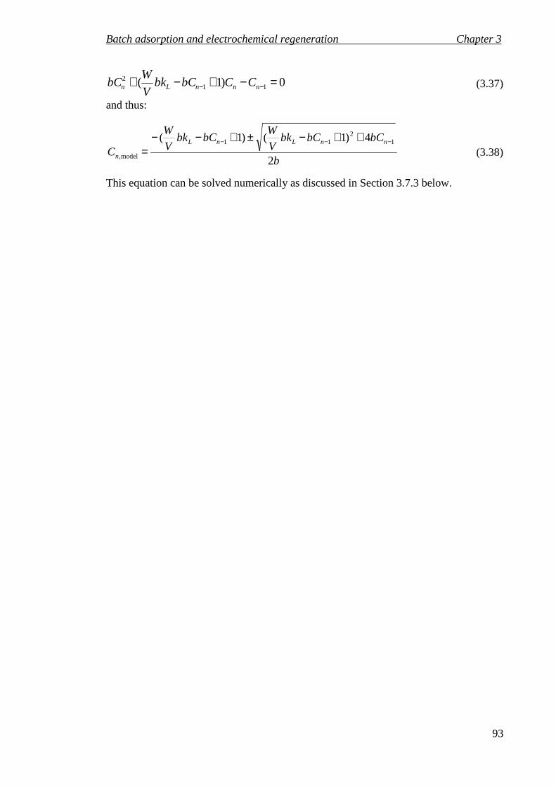
Batch adsorption and electrochemical regeneration Chapter 3
93
0)1( 112 =−+−+ −− nnnLn CCbCbk
V
WbC (3.37)
and thus:
b
bCbCbkV
WbCbk
V
W
CnnLnL
n 2
4)1()1( 12
11
model,
−−− ++−±+−−= (3.38)
This equation can be solved numerically as discussed in Section 3.7.3 below.
Batch adsorption and electrochemical regeneration Chapter 3
94
3.7.3 Numerical methodology
Excel's Solver is a numerical optimization add-in, distributed with Microsoft Excel,
which is a powerful analysis tool and used for optimization and simulation of business
and engineering models. It can be more powerful if used in conjunction with VBA, to
automate solving of multiple models which use different input parameters and
constraints (Billo, 2001). This numerical technique was developed by Frontline System,
Inc. (Solver.com) for solving the following problems:
• Linear programming (LP)
• Nonlinear optimization programming (NLP)
• Sequential quadratic programming (QP)
• Generalized reduced gradient (GRG)
• Mixed-integer optimization (MIP)
Equation (3.38) was used in Microsoft Excel to determine the concentration after each
stage of treatment for a given feed and mass of adsorbent. The solution was then
optimised using the Solver Add-In in Microsoft Excel using a forward derivative
Newton’s method with a convergence limit of 10−4 in order to calculate the amount of
adsorbent, W (g), required to achieve a given feed, percentage dye removal and number
of treatment stages. The target used for the solver was the minimization of the
normalised square error (Equation 3.40) between the required concentrations at stage (n)
(Equation 3.39) and the concentration calculated from the model (Equation 3.38), which
was achieved by adjusting the amount of adsorbent, W (g):
)100
Removal%1.( −= οCCn (3.39)
2
model,Error
−=
n
nn
C
CC (3.40)

Batch adsorption and electrochemical regeneration Chapter 3
95
3.8 Modelling results and discussion
Equation (3.38) was solved using the parameter values of the isotherm data b and kL at
0.31 L mg−1 and 0.987 mg g−1, respectively. The amount of adsorbent W was estimated
in the batch adsorber per unit volume of AV17 for 99, 98, 95, 90, 80, 70, 60, 50, 40, 30,
20 and 10% dye removal at different initial concentrations (55 – 680 mg L−1) using the
Solver tool in Microsoft Excel®. Figure 3.19 shows the amount of adsorbent per volume
of effluent treated required to remove dye at different initial concentrations of AV17 for
a five stage batch adsorber system of adsorption and electrochemical regeneration. The
model is consistent with the experimental data since the amount of Nyex®1000 required
per unit volume for 90% removal of AV17 dye solution of concentration 680 mg L−1
was 126 g L−1, which compares with 93 % removal achieved with 125 g L−1 for an
initial concentration of 668 mg L−1.
Figure 3.19: Amount of adsorbent required per unit volume of effluent treated against the percentage removal at different initial dye (AV17) concentrations for a five stage batch adsorption and regeneration system.
The experimental results discussed in Section 3.6.4 have been used to validate the
model (Equation 3.38). The accumulated percentage removal obtained from the model
and the experiment (Equation 3.41) is plotted for the five stages of adsorption and
electrochemical regeneration in Figure 3.20. It can be seen from this figure that the
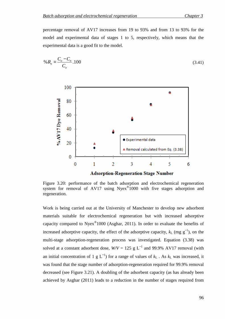
Batch adsorption and electrochemical regeneration Chapter 3
96
percentage removal of AV17 increases from 19 to 93% and from 13 to 93% for the
model and experimental data of stages 1 to 5, respectively, which means that the
experimental data is a good fit to the model.
100.%o
non C
CCR
−= (3.41)
Figure 3.20: performance of the batch adsorption and electrochemical regeneration system for removal of AV17 using Nyex®1000 with five stages adsorption and regeneration.
Work is being carried out at the University of Manchester to develop new adsorbent
materials suitable for electrochemical regeneration but with increased adsorptive
capacity compared to Nyex®1000 (Asghar, 2011). In order to evaluate the benefits of
increased adsorptive capacity, the effect of the adsorptive capacity, kL (mg g−1), on the
multi-stage adsorption-regeneration process was investigated. Equation (3.38) was
solved at a constant adsorbent dose, W/V = 125 g L−1 and 99.9% AV17 removal (with
an initial concentration of 1 g L−1) for a range of values of kL . As kL was increased, it
was found that the stage number of adsorption-regeneration required for 99.9% removal
decreased (see Figure 3.21). A doubling of the adsorbent capacity (as has already been
achieved by Asghar (2011) leads to a reduction in the number of stages required from

Batch adsorption and electrochemical regeneration Chapter 3
97
10 to 5, while an order of magnitude increase in kL would reduce the number of stages
required to 2. This could have a significant impact on the economics of the process.
Figure 3.21: Effect of the adsorptive capacity (kL) on the number of stages required for 99.9% removal of AV17 (with an initial concentration of 1 g L−1) using multi-stage adsorption-regeneration.

Batch adsorption and electrochemical regeneration Chapter 3
98
3.9 Conclusions
The conclusions that can be drawn from this Chapter are as follows:
3.9.1 Adsorption
The present study shows that Nyex®1000, a bisulphate graphite intercalation compound,
is capable of removing Acid Violet 17 from an aqueous solution with an equilibrium
time of about 60 min. The loading of dye on the adsorbent (mg g−1) was found to
increase with an increase in initial concentration and temperature. A pseudo second-
order model was found to provide a better fit to the kinetic data than a pseudo first-order
model, although the quality of the fit was relatively poor in both cases. This is in part
because the kinetics is relatively fast, and it is difficult to obtain accurate data at short
adsorption times. The rate constants obtained from the pseudo second-order model
obtained at a range of temperatures indicated the activation energy of order 4 kJ mol−1.
This low activation energy is characteristic of a diffusion-controlled, physisorption
process (Banerjee et al., 1997). The adsorption of Acid violet 17 onto Nyex®1000 was
observed to follow a Langmuir isotherm and the equilibrium loading of AV17 dye was
in the range 0.22 to 0.88 mg g-1 for equilibrium concentrations of 1.0 to 28.57 mg L−1
which suggests a monolayer coverage of the dye onto the adsorbent. The adsorption
equilibrium data was fitted to the Freundlich, Langmuir and Redlich-Peterson isotherm
models. The Langmuir and Redlich-Peterson models were found to fit the data better
than the Freundlich model. The parameters obtained indicated that the Redlich-Peterson
model could be simplified to the Langmuir model. The isotherm shape for a Langmuir-
type adsorption process was found to show a more favourable uptake at higher
concentrations and the experimental data found indicated a separation factor, RL, equal
to 0.06 which means that Nyex®1000 is effective for removal of AV17 from aqueous
solutions. The adsorbent capacity of Nyex®1000 for AV17 was found to increase with
decreasing solution pH for pH < 4. This adsorbent capacity was observed to be about
two and half times that of activated carbon in terms of the available surface area, mg
m−2, (see Table 3.5).
In addition, the kinetic and isotherm data obtained are shown to be suitable for the
development of a model of the continuous adsorption and regeneration apparatus
describe by Brown et al. (2007), and this is the subject of Chapter four. Additionally, a
Batch adsorption and electrochemical regeneration Chapter 3
99
flake GIC adsorbent with a large particle size, Nyex®1000, is suitable for process flow
application as it settles rapidly.
3.9.2 Regeneration Adsorbent development has conventionally aimed to develop either low cost materials
or high surface area, high capacity materials. However, the cost of regeneration of
porous adsorbents such as activated carbon is a significant issue. It has recently been
shown that low capacity graphite adsorbents can be regenerated rapidly and cheaply, so
that they can be regenerated and reused within the process (Brown et al., 2004c). This
study reports the first detailed study of the adsorption / regeneration characteristics of
one of these adsorbents: Nyex®1000, a graphite intercalation compound. The laboratory
scale batch regeneration tests demonstrated that the Nyex®1000 GIC adsorbent could be
fully regenerated with a charge of around 15 C g−1. This charge is of the correct order of
magnitude to suggest that the dye is mineralised during regeneration.
3.9.3 Multi-stage batch process In this work we report for the first time that a multi-stage batch treatment of water by
adsorption with electrochemical regeneration can be effective for the removal and
oxidation of dissolved organic contaminants. Multistage adsorption / regeneration was
shown to be effective for the removal of high concentrations of AV17 dye using
Nyex®1000 adsorbent which can be rapidly regenerated electrochemically. Removal of
93% of the dye from a solution containing 668 mg L−1 of AV17 was achieved after five
cycles of treatment with 125 g L−1 of Nyex®1000. A multi-stage design model for the
adsorption and electrochemical regeneration process for removal of a dye based on the
Langmuir equilibrium isotherm has been developed and this was used to predict the
dosage of adsorbent (W/V, g L−1) required to achieve a fixed percentage of dye removal
for a given number of adsorption / regeneration cycles. The model was found to be in
good agreement with the experimental results obtained for five stages of adsorption /
regeneration. Additionally, the average loading capacity was found to be approximately
1±0.05 mg g−1 at each stage which confirms the capacity of adsorbent value obtained
with the isotherms study (kL, Table 3.4). It was found that the predicted number of

Batch adsorption and electrochemical regeneration Chapter 3
100
stages of batch adsorption / regeneration required to achieve 99.9% AV17 removal was
halved when the adsorptive capacity of the Nyex®1000 was doubled. This finding
confirms that development of adsorbents which can be regenerated electrochemically
with increased capacity compared to Nyex®1000 could significantly improve the
economics of the process.

Continuous adsorption and electrochemical regeneration Chapter 4
101
CHAPTER 4
CONTINUOUS ADSORPTION AND ELECTROCHEMICAL REGENERATION
In this Chapter, water treatment by continuous adsorption and electrochemical
regeneration is evaluated. Relevant literature is reviewed, the behaviour of different
types of adsorber (fixed bed, fluidized bed and airlift) are discussed and residence time
distributions (RTD) are explained. The methodology for characterisation of the
continuous adsorption process, including RTD and adsorbent circulation are described.
In addition, the experimental apparatus and procedures for studying the adsorber
performance and behaviour are explained and discussed. Based on the data obtained a
design model for continuous waste water treatment by adsorption with electrochemical
regeneration is developed. A plug flow reactor model has been developed in order to
study the possibility of process improvement. Sensitivity studies to evaluate the effect
of key parameters on the performance of the process of water treatment by adsorption
with electrochemical regeneration are presented and discussed.
4.1 Adsorber background
Adsorption is a separation process in which components of a fluid phase (organic
materials in this case) are transferred and bonded to the surface of a solid adsorbent
without any chemical change (Demirbas et al., 2008). This process can be conducted
with the adsorbent in a batch, continuous flow stirred tank, fixed bed, or fluidized bed
adsorber (Culp et al., 1978).
Fixed bed adsorption processes are widely used throughout the chemical process and
other industries such as the pharmaceuticals, wastewater treatment and environmental
technology industries (Pohorecki, 2002). This process can be operated as a single unit or
multiple units in series and / or parallel. The main advantages of a fixed bed adsorber
include being its simple operation, relatively low cost, and the ease of scale up from
laboratory to full scale operation (Chern and Chien, 2002), whereas the drawbacks are
large pressure drop across the bed and the need for more than one bed of adsorbent for a
Continuous adsorption and electrochemical regeneration Chapter 4
102
continuous process (the simplest set up requires two beds in which one undergoes
adsorption while the other undergoes regeneration) and the potential for short contact
times between the adsorbent and the water to be treated due to channels occurring along
the bed wall. Many researchers have investigated the adsorption of organic dyes from
polluted water onto activated carbon using fixed bed systems. For example, Walker and
Weatherley (1998) studied the adsorption of an acid dye from wastewater arising from a
nylon carpet printing plant onto granular activated carbon. They found that the desired
reduction in acid dye effluent concentration, over a sustainable period of time, required
low linear flow rates and the use of a fine particle size of adsorbent. However, the
problems associated with fixed beds are significantly reduced in fluidized bed adsorbers
(Veeraraghavan et al., 1989). The potential advantages of a fluidized bed over the fixed
bed is that intraparticle mass transport resistance is much lower (McKay, 1988);
(Veeraraghavan et al., 1989). This phenomenon is possibly due to axial mixing taking
place between solid and liquid phases in the fluidized bed adsorber.
Adsorbers may be divided into three groups depending on the method of supplying
energy:
• Mechanically-driven adsorbers e.g. tanks with a stirrer
• Hydraulic-driven adsorbers e.g. fluidised bed
• Pneumatically-driven ones e.g. pulsed flow columns and air-lift adsorbers.
Due to the operational complexity and limitations in terms of the removal of organic
dyes, researchers have been encouraged to look for new more efficient techniques
(Mohanty et al., 2008). Airlift reactors have been applied as an alternative to fixed,
moving, and fluidized bed techniques in wastewater treatment and biological processes
as they provide efficient contacting for mass and heat transfer (Demming et al., 2008);
(Heijnen et al., 1991). The three phase airlift reactor (air-liquid-solid) is a pneumatically
agitated system characterised by fluid circulation in a defined recirculation mode
(Merchuk and Siegel, 1988). The first airlift reactor was constructed by Lefrancois et al.
(1955). The main advantages of air lift reactors are a simple mechanical design, low
energy input (they use about three fold less energy than other multiphase reactors), low
shear rate, and good mixing (Chisti et al., 1988); (Filipkowska, 2004). However, the
drawbacks of the airlift reactor include the possibility of foaming and limited
application for media of low viscosity (Pohorecki, 2002). These disadvantages are not

Continuous adsorption and electrochemical regeneration Chapter 4
103
normally significant issues for adsorption processes (Filipkowska and Waraksa, 2008).
Air lift reactors are classified into two main categories based on the configuration of the
recirculation: internal-loop and external-loop air lift reactors, as illustrated in Figure 4.1.
The main difference between these categories is the level of the liquid-gas separation
achieved (i.e. the design of the gas-liquid separator). The external loop air lift reactor
has a disengagement section and as such is beneficial for mixing and heat transfer in
reactors, due to the gas-liquid separation achieved. However, the internal loop air lift
reactor has the downcomer integrated with the riser in the same vessel and there is less
opportunity for gas disengagement. Consequently perfect liquid-gas separation is not
achieved (Merchuk and Siegel, 1988). However, internal air lift reactors have a number
of advantages including a small footprint and good gas-liquid mass transfer.
Generally, all air lift reactors consist of four distinct sections or compartments with
different flow characteristics (Merchuk and Siegel, 1988):
• Riser: at the bottom of this section, the gas is injected and the flow of the gas
and liquid is co-current in an upward direction.
• Downcomer: this is parallel to the riser and the flow of the liquid is
predominantly downward.
• Base: the bottom connection section between the downcomer and riser does not
have a significant effect on the overall reactor performance, but the design of
this section might influence the solid phase flow, gas holdup and liquid velocity.
• Disengagement: this section at the top of the reactor connects the riser and
downcomer, allowing gas disengagement and liquid recirculation.

Continuous adsorption and electrochemical regeneration Chapter 4
104
Air inlet
Air inlet Air inlet Air inlet Air inlet
Ris
er
Ris
er
Ris
er
Ris
er
Dow
ncom
er
Dow
ncom
er
Dow
ncom
er
Dow
ncom
er
Air exit Air exit Air exit
(i) (ii)
(b)
(iii)
(a) (a) (a)
Ris
er
Ris
er
Ris
er
Ris
er
(a)
Dow
ncom
er
Dow
ncom
er
Dow
ncom
er
Air exit
Dow
ncom
er
Air exit
Air inlet
Ris
er
(iv)
Figure 4.1: Airlift reactors: (a) the four main types of internal air loop reactor: (i) split cylinder, (ii) concentric draught-tube and (iii) single-annulus, (iv) multiple-annulus; and (b) external loop airlift reactor.
Continuous adsorption and electrochemical regeneration Chapter 4
105
The following sections briefly described the main categories of air lift reactor:
4.1.1 Internal loop airlift reactor
An internal loop airlift reactor is a cylindrical or rectangular vessel separated on the
inside with a baffle into a riser and a downcomer in order to establish liquid circulation.
The advantages of this design include relatively low shear stress conditions, and high
gas-liquid mass transfer due to increased contact area between gas and liquid, thereby
increased gas conversion per pass (Sun et al., 2006). There are different types of internal
loop airlift reactors as follows:
4.1.1.1 Concentric or annulus airlift reactor
These consist of an internal cylindrical draft tube, which is enclosed in a cylindrical
column. In an annulus air lift reactor the downcomer is in the middle with the riser in
the annulus, while for the concentric airlift reactor the riser is in the middle and the
downcomer is in the annulus. The continuous process for water treatment by adsorption
with electrochemical regeneration developed in Manchester (the Arvia® process) is
similar to an annulus airlift reactor, but with a rectangular rather than cylindrical
construction. This design enables continuous circulation of the adsorbent, with the
advantages of relatively low shear stresses and good mass transfer rates between the
solid and liquid (Sun et al., 2006) due to the agitation provided by the rising bubbles of
air.
4.1.1.2 Multiple airlift reactors
Multiple airlift reactors provides an improved level of mixing if required and offers a
development upon the annulus air lift reactor design. As illustrated in Figure 4.2, the
multiple air lift reactor contains a number of annulus air lift reactors in series,
incorporated into one reactor. The concentrically placed reactors create a new type of
geometry for internal air lift reactors. The cylindrical baffles split each compartment
creating a riser and downcomer (Bakker et al., 1993). According to Verlaan et al. (1989)
the flow behaviour of annulus air lift reactors is like a stirred tank reactor, whereas the
multiple air lift reactor behaves like an aerated plug flow reactor, or a series of stirred
tank reactors (Bakker et al., 1993). The multiple air lift reactor design can be adapted

Continuous adsorption and electrochemical regeneration Chapter 4
106
with two or three phase mixing, and a rectangular geometry has been suggested for
wastewater treatment applications (Bakker et al., 1993).
Baffle
Side View
Top View
Medium in
Out Out
Gas inlet
Gas spargers
Figure 4.2: Schematic diagram showing side and top views of a three compartment multiple airlift reactor (Bakker et al., 1993).
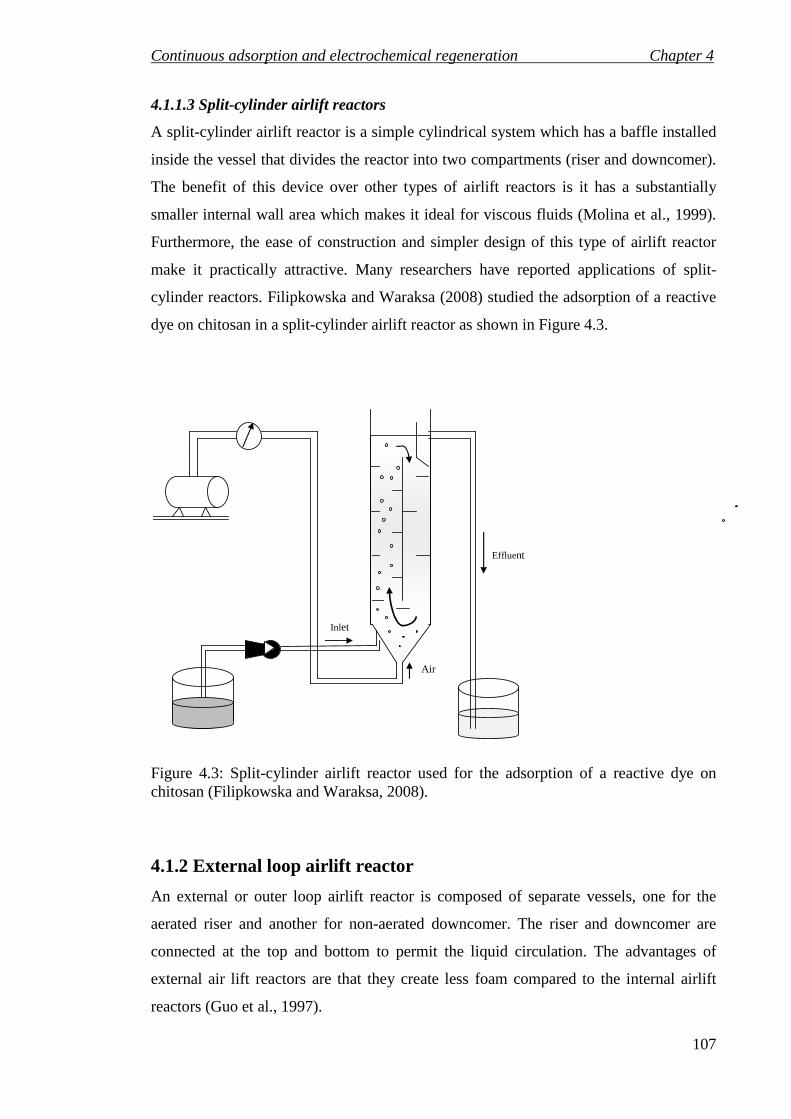
Continuous adsorption and electrochemical regeneration Chapter 4
107
4.1.1.3 Split-cylinder airlift reactors
A split-cylinder airlift reactor is a simple cylindrical system which has a baffle installed
inside the vessel that divides the reactor into two compartments (riser and downcomer).
The benefit of this device over other types of airlift reactors is it has a substantially
smaller internal wall area which makes it ideal for viscous fluids (Molina et al., 1999).
Furthermore, the ease of construction and simpler design of this type of airlift reactor
make it practically attractive. Many researchers have reported applications of split-
cylinder reactors. Filipkowska and Waraksa (2008) studied the adsorption of a reactive
dye on chitosan in a split-cylinder airlift reactor as shown in Figure 4.3.
Figure 4.3: Split-cylinder airlift reactor used for the adsorption of a reactive dye on chitosan (Filipkowska and Waraksa, 2008).
4.1.2 External loop airlift reactor
An external or outer loop airlift reactor is composed of separate vessels, one for the
aerated riser and another for non-aerated downcomer. The riser and downcomer are
connected at the top and bottom to permit the liquid circulation. The advantages of
external air lift reactors are that they create less foam compared to the internal airlift
reactors (Guo et al., 1997).
Inlet
Air
Effluent

Continuous adsorption and electrochemical regeneration Chapter 4
108
4.1.3 Summary
In summary, adsorption processes can be conducted using a range different techniques
(e.g. fixed bed, moving bed, fluidized bed, airlift adsorber, etc.) and all have both
advantages and disadvantages; hence there is no obvious stand out technique. Airlift
systems allow for better mixing to take place between the solid (adsorbent) and the
liquid (polluted water) without additional mechanical complication. Internal loop airlift
reactors not only have milder shear stresses than external airlift reactor, but they also
have good mixing properties (Mohanty et al., 2008). However, the external loop airlift
reactor could be used due to creating less foam compared to the other types. This type
of system could be considered as an option for process improvement.
Continuous adsorption and electrochemical regeneration Chapter 4
109
4.2 Process design and characterisation Brown et al. (2007) have patented a continuous process with adsorption and
electrochemical regeneration occurring in the same device. The process has been named
‘the Arvia® Process’, and uses the principle of air-lift circulation for multiphase
contacting of the graphitic adsorbent with the polluted water (described below in section
4.2.2). The design of such a continuous flow process depends upon two key factors; the
kinetics (rate equations) and backmixing or dispersion behaviour. In this case, the first
factor requires consideration of the amount of the contaminated adsorbate on the
adsorbent material at equilibrium and also requires a study of the kinetics of adsorption
(as discussed in Chapter 3) to provide information about the rate of adsorption. The
dispersion behaviour is used to represent the combined action of a number of
phenomena, namely molecular diffusion, turbulent mixing, and non-uniform velocities,
which give rise to a distribution of residence time in the reactor (discussed below in
section 4.2.1).
4.2.1 Process characterisation
A discussed above a design model of a three phase airlift adsorber requires information
regarding the dispersion behaviour and rate of adsorption. The dispersion information
can be obtained through characterisation or diagnosis of the flow behaviour in the
adsorber using experimental or computational fluid dynamics studies of the residence
time distribution (RTD). The RTD is a simple tool to characterise the flow and
dispersion behaviour in flow processes (Claudel et al., 2003).
4.2.1.1 RTD background
There are two main ideal reactor models that are used for description of flow behaviour.
The two categories of ideal reactor are the continuous stirred tank reactor (CSTR) and
the plug flow reactor (PFR). In an ideal CSTR the reactant concentration is uniform
throughout the vessel. In real stirred tank reactors non-ideal behaviour can occur with
the formation of dead zones, which do not mix with the fluid in the rest of the vessel, or
near feed points, where reactant concentration may be relatively high before they are
mixed into the vessel volume. An ideal PFR is a tubular reactor where all reactant and
product molecules have the same flow rate at any position along the axis (Fogler, 1999);

Continuous adsorption and electrochemical regeneration Chapter 4
110
(Levenspiel, 1999). In an ideal PFR there is perfect mixing in the radial direction by no
mixing in the axial direction. In practical tubular reactors, non-ideal behaviour arises
due to turbulent mixing or molecular diffusion which causes molecules to mix in the
axial direction.
Deviations from ideal reactor behaviour pose several problems in the design and
analysis of reactors. Figure 4.4 presents the possible deviations from ideality namely
‘dead zones’ where little mixing occurs and ‘short circuiting’ or ‘by pass’ flows. To
describe these deviations from ideality, three concepts are generally used, which are
regarded as characteristic of mixing (Levenspiel, 1999):
• The residence time distribution (RTD).
• The quality of mixing.
• The model used to describe the process.
The residence time is the time an element of fluid spends inside the reactor. Each
element of fluid may spend a different time inside the tank and the distribution of
residence time of the elements goes to make up the residence time distribution. The
RTD can be used to characterise and diagnose the flow in a nonideal reactor. It is also
considered a useful tool in the design and modelling of reactors. The RTD can be
determined by the so-called "stimulus response" technique for a flowing fluid through a
Figure 4.4: Real flow patterns exist in process equipment (Levenspiel, 1999).
Short circulating
Stagnant (dead) zone

Continuous adsorption and electrochemical regeneration Chapter 4
111
reactor (Shah, 1979). The principle idea of this technique is to inject a tracer in the form
of a step or pulse at the entrance of the reactor and measure its concentration at the
outlet as a function of time (Levenspiel, 1999). A proper choice of this tracer can be
identified by the following desirable characteristics:
• The physical properties of the tracer should be similar or closely follow those
of the mixture under treatment and be completely soluble in the mixture.
• The tracer should not react with or be absorbed by any solid surfaces in the
reactor.
• The tracer should be easily detectable in small concentrations.
• The tracer should not change from phase to phase during the experiment.
• The cost of the tracer and detection device should be relatively cheap.
A radioactive tracer offers an advantage for measuring the RTD of a very fast-moving
phase as a scintillation detection counter can be interfaced with very rapid recording
systems. In the liquid phase, usually the tracer (e.g. NaCl, H2SO4, etc.) can be detected
by directly inserting a probe into the reactor outlet and continuously monitoring the
concentration by means of electrical conductivity. Table 4.1 presents some of the tracers
used for liquid phase.
Table 4.1:Tracer types employed in air water system and detection devices (Shah, 1979).
System Tracers Detection devices Reactor
Air- water
Air- water
Air- water
Air- water
HCl
H2SO4
NaCl
Methylene
Blue dye
Electrical conductivity
Electrical conductivity
Electrical conductivity
Spectrophotometer
Packed bed
Packed bed and bubble column
Packed bed
Packed bed
Based on the data shown in Table 4.1 for an air-water system, sodium chloride has been
selected as a tracer material to study the RTD in this thesis. Using this material, the
detection device can measure the electrical conductivity of the effluent to determine the
outlet concentration. Additionally, this tracer is relatively cheap, easily detectable at
relatively low concentrations and has nearly no adsorption onto carbon adsorbent
Continuous adsorption and electrochemical regeneration Chapter 4
112
(Wanko et al., 2010) .The stability of sodium chloride in the adsorption process will be
investigated to confirm it is not adsorbed onto Nyex®1000 adsorbent used in this study.
The object of the RTD experiments is to assess the degree of dispersion and therefore to
predict the effect on reactor performance. The characterisation of reactor RTD
behaviour has become a valuable technique in aiding the design of chemical reactors,
aeration tanks for sewage treatment and in water treatment processes. Investigators of
RTD in continuous flow processes have applied various techniques to determine the
tracer response in the outlet flow. Normally this technique involves the injection of
known amounts of tracer solution in the form of a pulse, step, sinusoid, or ramp in the
inlet stream, followed by detecting its concentration as a function of time in the outlet
stream.(Shah, 1979) The position of injection and detection points should be very close
to the reactor so that no dispersion carries the tracer materials across system boundaries.
The two most common methods used are the pulse and step tracer input, and the typical
concentration curves at the inlet and outlet of the reactor are shown in Figure 4.5
(Fogler, 1999).

Continuous adsorption and electrochemical regeneration Chapter 4
113
Step injection
Pulse response
Cin
0 t
Cmax
0
Step response
Cout
Pulse injection
Reactor
Detection
Effluent
Cout
t 0 0
Cin
Injection
Influent
Figure 4.5: Various tracer injection – response RTD measurements techniques (Fogler,
1999).
Pulse tracer input
A quantity of tracer is injected at the inlet of a system over a period of time which is
very short compared to the mean residence time, and the concentration of the tracer in
the outlet stream is measured as a function of time. In order to interpret the data, it is
assumed that at the inlet and outlet: there is constant flow rate and fluid density, only
one phase is flowing into the system i.e. the tracer solution, no diffusion takes place
across the system boundaries, and the velocity profiles are flat. Furthermore, it is
assumed that the magnitude of the tracer response at the outlet is directly proportional to
the amount of tracer injected, the dispersion behaviour of the tracer is identical to the

Continuous adsorption and electrochemical regeneration Chapter 4
114
process fluid and that the there is no consumption or generation of tracer within the
system (Kayode Coker, 2001).
This technique has been used by many researchers. For example, pulse input RTD
characterisation has been performed by Saravanathamizhan et al. (2008) to diagnose the
electrolyte dispersion characteristics of a continuous stirred tank electrochemical reactor
(CSTER). Acid Red 88 dye solution was injected as a pulse input to the reactor and the
outlet concentration was analyzed as function to the time using a colorimeter. A three
parameter model was proposed to describe the electrolyte flow in the CSTER consisting
of active, dead and bypass zones with exchange flow between dead and active zones.
The drawbacks of the pulse injection technique are that the injection must be achieved
in a very short time, the amount of tracer used should be known, and inaccuracy may
result when the concentration versus time curve has a long tail. (Fogler, 1999).
However, one advantage of this technique is that it can be used to minimize the cost, if
the tracer is very expensive (Fogler, 1999).
Step tracer input
The step tracer input residence time experiment can be performed if the feed to a reactor
is switched from ordinary fluid to a fluid containing a known concentration of a tracer
and the concentration of the tracer at the reactor outlet monitored as a function of time
until the concentration of tracer at the outlet of the reactor is the same as that at the inlet.
A step tracer input is often used if the tracer is cheap or pleasant (e.g. non radioactive
tracers). Advantages of using a positive step in the RTD measurement are that it is
easier to carry out experimentally than a pulse test and the total amount of tracer
injected in the stream feed over the period of the experiment does not have to be known
as it does in the pulse test. On the other hand, the drawbacks to this approach are that it
is difficult to maintain a constant tracer concentration in the feed, the RTD is obtained
by differentiating the outlet tracer concentration versus time data which can lead to
error, and that a large amount of tracer is required (Fogler, 1999).

Continuous adsorption and electrochemical regeneration Chapter 4
115
4.2.1.2 Fundamentals of RTD theory In pulse input oN mol of tracer are injected and the effluent concentration is measured.
The amount of tracer material that has spent an amount of time between t and tt ∆+ in
the reactor is (Fogler, 1999),
tQCN t ∆=∆ (4.1)
where Q is the effluent volumetric flow rate.
The fraction of material that has spent in the reactor between t and t + ∆t for pulse input
is:
tEN
Nt
o
∆=∆ (4.2)
where Et is the residence time distribution function of a real reactor also called the exit-
age distribution function and equal to ot NQC
If oN is not known directly, it can be calculated from outlet concentration
measurements by summing up all the amount of material, so we can rewrite Equation
(4.1) in integral form:
dtCQN t∫∞
=0
(4.3)
Combining Equations (4.1), (4.2) and (4.3) and rearranging, we obtain:
∫∞=
0
dtC
CE
t
tt (4.4)
The integral in the denominator is the area under C-curve which is equal to ∑ ∆i
ti tC
and thus equal to QNo , hence the exit age distribution becomes,
o
tt N
QCE = (4.5)
Combining Equations (4.3) and (4.5), it can be shown that:
∫∞
=0
1dtEt (4.6)
The effective mean residence time is thus calculated using Equation (4.7), and this can
be compared to the expected value given by the ratio V/Q (V, is the total reactor

Continuous adsorption and electrochemical regeneration Chapter 4
116
volume). Specific problems of by-pass and/or dead (stagnant) volumes formed within
the real reactor can be detected by this comparison.
∫∞
=′0
dttEt t (4.7)
For the step input method the concentration of tracer is kept constant until the outlet
concentration equals the inlet concentration. The fraction of effluent which has been in
the reactor for a time less than t is called the cumulative distribution function Ft.
∫∞
=−0
1 dtEF tt (4.8)
The RTD is a probability density function, hence it can be characterised using statistical
moments which are often used to compare RTD’s instead of comparing the entire
distribution (Wen and Fan, 1975). The mean residence time (t ′ ), variance ( 2σ ),
skewness (s3) and coefficient of variation (Cv) are statistical moments defined as
(Levenspiel, 1999); (Harris et al., 2003):
τ≅≅∆
∆≅=′∑
∑
∫
∫∞
∞
Q
V
tC
tCt
dtC
tCdt
t
iii
iiii
t
0
0 (if it∆ is constant) (4.9)
2
22
0
0
2
2
0
2
)()(
)( ttC
tCt
tC
tCtt
dtC
dtCtt
dtEtt
iit
iiti
iii
iiii
t
t
t
i
i
′−∆
∆≅
∆
∆′−≅
′−=′−=
∑
∑
∑
∑
∫
∫∫ ∞
∞
∞
σ (4.10)
∫∞
′−=0
32/3
3 )(1
dtEtts tσ (4.11)
To characterise the RTD, the coefficient of variation is also used and this is defined as
(Harris et al., 2003):
tCv ′
= σ (4.12)
For RTD studies, the first two statistical moments, the mean residence time and the
variance of the RTD are the most important, and in this study t′ and σ have been used to
characterise the RTD.

Continuous adsorption and electrochemical regeneration Chapter 4
117
RTD in ideal reactors:
For a CSTR, a material balance on the tracer that has been injected in the form of a
pulse input gives:
τtt eCC −= 0 (4.13)
whereτ is the space time and equal to V/Q and Co is initial concentration of tracer
(given by No / V).
Substituting Equation (4.13) in to Equation (4.4):
∫∞
−
−
=
0
0
0
dteC
eCE
t
t
tτ
τ
(4.14)
Co is constant, hence Equation (4.14) becomes:
τ
τt
t
eE
−
= (4.15)
In order to directly compare the flow behaviour or performance inside reactors of
different sizes, frequently a normalized RTD is used instead of the exit age distribution
function, Et.
Defining the parameter θ as equal to t/τ, which represents the number of reactor
volumes of fluid based on entrance conditions that have flowed through the reactor in
time, for a CSTR we obtain:
θθ τ −== eEE t. (4.16)
Equation (4.9) has shown that in general the mean residence time t ′ in a reactor is equal
to V/Q or τ. Applying this definition of a mean residence time to the RTD for a CSTR,
gives:
ττ
τ ==′ ∫∞
−
0
tet
t (4.17)
In practical (non-ideal) reactors Equation (4.17) may not be valid and therefore there
may be a difference between the mean residence time and the space time.
Determining the second moment (variance) of the RTD for a CSTR we obtain:
∫∫∞
−∞
− =−=−=0
222
0
22 )1(
)( ττττσ τ dxexdte
t xt (4.18)
and thus, τσ =
Continuous adsorption and electrochemical regeneration Chapter 4
118
For a PFR, all the molecules leaving have spent exactly the same amount of time within
the reactor. The RTD function of a PFR is thus a spike which has infinite height and
zero width, whose area is equal to one. The spike can be represented mathematically by
the Dirac delta function:
)( τδ −= tEt (4.19)
∫∫∞
∞−
∞
=−==′ ττδ dtttdttEt t )(0
(4.20)
All the material has spent precisely the same time in the reactor, so the variance of the
RTD is zero:
∫∫∞∞
=−−=′−=0
2
0
22 0)()()( dtttdtEtt t τδτσ (4.21)
One parameter models:
Reactor models are useful for diagnosing flow behaviour and scale up in a real reactor.
A range of models can be used to describe the RTD of real (non-ideal) reactors. One
parameter models that can be used to describe the mixing behaviour or interpret RTD
deviations from ideal reactors (CSTR, PFR) are the tanks in series model and the
dispersed plug flow model. For the dispersed plug flow and tanks in series models, the
Peclet number (Pe) and the number of tanks (nT) are the single parameters that are used
to characterise the RTD, respectively (Saravanathamizhan et al., 2010). These models
preclude the requirement of applying computational fluid dynamics (CFD) by limiting
their application to a single characteristic length (Martin, 2000).
The dispersed plug flow model is one of the most widely used models in RTD studies.
Suppose an ideal pulse of tracer is injected into a tubular reactor, and the pulse spreads
as it passes through the reactor. The tracer spreads in the upstream and downstream
directions away from the centre of the original pulse due to molecular diffusion, non-
uniform velocities, and turbulent mixing. The longitudinal dispersion coefficient, D (m2
s−1) is used to characterised the spreading (dispersion) of the tracer cloud. Thus, a large
D indicates a rapid dispersion of the tracer, while a small D means slow dispersion and
D = 0 indicates no dispersion (and hence plug flow). To characterize the dispersion in
the reactor, the longitudinal Peclet number, uL/D, is often used, where u is the
superficial fluid velocity (m s−1) and L is the length of the reactor (m). The Peclet
number can be evaluated from the shape of the tracer curve as it passes the exit (i.e.

Continuous adsorption and electrochemical regeneration Chapter 4
119
from the RTD) of the reactor by calculation of the mean residence time (t ′ ) and the
variance of the RTD ( 2σ ) from Equations (4.9) and (4.10), respectively. Normally, the
dispersion of axial mixing in streamline flow of fluid through pipes is mainly due to
fluid velocity gradients, whereas radial mixing is due to molecular diffusion. To
describe the dispersion of the tracer in the axial direction, a Fickian dispersion equation
is used (Levenspiel, 1999):
2
2
x
CD
t
C
∂∂=
∂∂
(4.22)
In terms of the normalized form where Ltut == τθ and Lxutz )( += , the basic
differential equation representing the tracer dispersion becomes
z
C
z
C
uL
DC
∂∂−
∂∂=
∂∂
2
2
θ (4.23)
where =uLD 1 / Pe = DN , ND is the vessel dispersion number, and Pe is the Peclet
number. The Peclet number is defined as the rate of transport by convection (uL)
divided to the rate of transport by dispersion (D).
Two types of boundary conditions are considered, namely open and closed vessels. The
first boundary condition is that in which the flow is undisturbed as it passes the inlet and
outlet boundaries, whereas the secondary boundary condition dispersion occurs across
inlet and outlet boundaries.
Open dispersion model
The analytical solution for Equation (4.23) was published by Levenspiel and Smith
(1957) for “open” boundary condition using a dimensionless form as shown in Equation
(4.24).
−−
= θθ
θ πθ4
)1(Pe
,
2
.Pe
2
1eE o (4.24)
with normalized mean and variance
Pe2
1+=oθ (4.25)
+=PePe4
122
,σ θ o (4.26)
The subscript o indicates open boundary conditions.

Continuous adsorption and electrochemical regeneration Chapter 4
120
Closed dispersion model
This system was treated with closed boundary conditions in which the flow approaches
the inlet to the reactor in an idealised plug flow ( ∞=Pe ), transforms to dispersed flow
within the reactor and returns to idealised plug flow at the outlet. The analytical solution
for Equation (4.23) was not reported by Levenspiel (1999) for a closed system.
However, the analytical solution for this equation was published by Thomas and McKee
(1944) with closed boundary conditions in a dimensionless form. Their solution was
reproduced by Yagi and Miyauchi (1953) with in a slightly different form:
( )
+
++= ∑
∞=
=
+−
nnn
n
n n
nc
n
E αααα
ααθ
θ 2sin
2cos
4)1(2
12
2/112
,
2
PePePe
ePePe
(4.27)
where αn is the positive root of Equation (4.28).
( )1
2
2
Petan
2 −=
n
nn α
αα (4.28)
The normalized mean residence time and variance of the RTD are shown in Equations
4.29 and 4.30, respectively.
1
)1(Pe
)1(Pe4
1
122
=
+
+=∑
∑∞=
=
∞=
=n
n n
n
n
n n
n
c K
K
α
αθ (4.29)
( )2
2Pe
4
1
133
2, Pe
11
Pe
21
)1(Pe
)1(Pe32
t
eK
K
n
n n
n
n
n n
n
c ′=
−−=−
+
+=−
=
=
∞=
=
∑
∑ σ
α
ασ θ (4.30)
where nK is given:
( ) 41Pe
Pe22 ++
=n
nnK
αα
(4.31)
The subscript c denotes closed boundary conditions.

Continuous adsorption and electrochemical regeneration Chapter 4
121
Tank in series model
This model describes the flow in a non-ideal reactor by considering it to be discretised
into a series of equal sized CSTRs; each independent of those preceding or following it
(Martin, 2000). Integration of a simple dynamic tracer mass balance on series of nT
CSTRs gives the system RTD function:
( ) )(1, e
)!1(θ
θ θ TT
Tnn
T
nT
T n
nE −−
−= (4.32)
with mean and variance
1=Tθ (4.33)
TT n
12, =θσ (4.34)
The subscript T indicates the tanks in series model.
In summary, the tanks in series model is easier to apply compared to the open or closed
dispersed plug flow models due to its relatively simpler mathematical definition. The
tanks in series model can be used for reactors with any kinetics and any configuration of
compartments with or without recycle (Martin, 2000). Additionally, defining the entry
and exit boundary conditions is not critical, as it is in the dispersed plug flow model.
However, this model has a significant drawback when nT is small due to the integer
constraint, i.e. only whole numbers of tanks are allowed. However, Martin (2000) has
shown that the RTD can be characterised with a non-integer number of tanks.
4.2.2 Process design
4.2.2.1Description Experiments were carried out using a prototype developed at the University of
Manchester and a process unit constructed by Arvia® Technology Ltd. The
experimental methods for water treatment by continuous adsorption and electrochemical
regeneration were carried out in two different designs of the Arvia® Process, which are
similar to an annulus air lift reactor (see Figure 4.6 and 4.7), a type of internal air lift
reactor. The air lift system was used to circulate the adsorbent, from the settling and
regeneration zones, back out to the adsorption zone. In these devices, which are
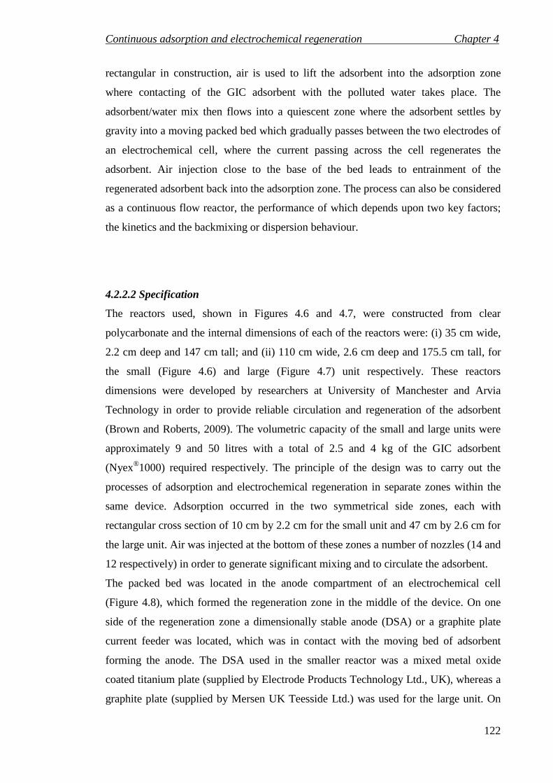
Continuous adsorption and electrochemical regeneration Chapter 4
122
rectangular in construction, air is used to lift the adsorbent into the adsorption zone
where contacting of the GIC adsorbent with the polluted water takes place. The
adsorbent/water mix then flows into a quiescent zone where the adsorbent settles by
gravity into a moving packed bed which gradually passes between the two electrodes of
an electrochemical cell, where the current passing across the cell regenerates the
adsorbent. Air injection close to the base of the bed leads to entrainment of the
regenerated adsorbent back into the adsorption zone. The process can also be considered
as a continuous flow reactor, the performance of which depends upon two key factors;
the kinetics and the backmixing or dispersion behaviour.
4.2.2.2 Specification
The reactors used, shown in Figures 4.6 and 4.7, were constructed from clear
polycarbonate and the internal dimensions of each of the reactors were: (i) 35 cm wide,
2.2 cm deep and 147 cm tall; and (ii) 110 cm wide, 2.6 cm deep and 175.5 cm tall, for
the small (Figure 4.6) and large (Figure 4.7) unit respectively. These reactors
dimensions were developed by researchers at University of Manchester and Arvia
Technology in order to provide reliable circulation and regeneration of the adsorbent
(Brown and Roberts, 2009). The volumetric capacity of the small and large units were
approximately 9 and 50 litres with a total of 2.5 and 4 kg of the GIC adsorbent
(Nyex®1000) required respectively. The principle of the design was to carry out the
processes of adsorption and electrochemical regeneration in separate zones within the
same device. Adsorption occurred in the two symmetrical side zones, each with
rectangular cross section of 10 cm by 2.2 cm for the small unit and 47 cm by 2.6 cm for
the large unit. Air was injected at the bottom of these zones a number of nozzles (14 and
12 respectively) in order to generate significant mixing and to circulate the adsorbent.
The packed bed was located in the anode compartment of an electrochemical cell
(Figure 4.8), which formed the regeneration zone in the middle of the device. On one
side of the regeneration zone a dimensionally stable anode (DSA) or a graphite plate
current feeder was located, which was in contact with the moving bed of adsorbent
forming the anode. The DSA used in the smaller reactor was a mixed metal oxide
coated titanium plate (supplied by Electrode Products Technology Ltd., UK), whereas a
graphite plate (supplied by Mersen UK Teesside Ltd.) was used for the large unit. On
Continuous adsorption and electrochemical regeneration Chapter 4
123
the other side of the regeneration zone was a microporous polyethylene membrane
(Daramic®350, Grace GmbH, Germany) which separated the adsorbent from a
perforated 316L stainless steel cathode for the small unit and graphite cathode for the
large unit. The anode and cathode electrodes were both 12 cm wide by 60 cm in height,
and the distance between the anode current feeder and the membrane (i.e. the depth of
the regeneration zone) was 22 and 26 mm for the small and large unit respectively. The
cathode compartment was filled with acidified 0.3 wt% NaCl solution to provide good
conductivity.

Continuous adsorption and electrochemical regeneration Chapter 4
124
Downcomer
10 cm
5 cm
129 cm
Air injection
I7 I1 I1 I7
moving bed of
adsorbent
Quiescent region
Settlement zone
Influent Influent
Drainage valve
A
A
Adsorption zones
(a)
12 cm
Air disengagement
Outlet for treated water
Regeneration zone
Figure 4.6: (a) Schematic diagram and (b) annotated photograph of the smaller air lift reactor for continuous water treatment by adsorption with electrochemical regeneration.
Regeneration Zone
Adsorption Zone
Outlet for treated water
Settlement Zone
Quiescent region
Drainage Valve
Catholyte outlet
(b)

Continuous adsorption and electrochemical regeneration Chapter 4
125
Influent Influent
Air injection Air injection
Effluent
Air disengagement
Air disengagement
Regeneration zone
Adsorption zone
Settlement zone
Riser Riser
Dow
ncomer
Quiescent region
Top drainage valve
Bottom drainage valve
148 cm
9 cm
47cm
I6 I6 I1 I1
12cm
A
A
(a)
Figure 4.7: (a) Schematic diagram and (b) annotated photograph of the larger air lift reactor for continuous water treatment by adsorption with electrochemical regeneration.
Flow meters
Adsorption zone
Regeneration zone
InfluentInfluent
Air injection
effluenteffluent
(b)

Continuous adsorption and electrochemical regeneration Chapter 4
126
Catholyte in
Catholyte out Adsorbent bed
metal oxide coated titanium anode
Membrane
Perforated 316L St.St. Cathode
hydrogen
(a)
Catholyte in
Catholyte out +
Hydrogen
Adsorbent bed
Graphite Anode
Membrane
Graphite Cathode
(b)
Figure 4.8: Schematic diagram of the electrochemical regeneration zone for (a) and (b) showing a cross section through line A-A in Figure 4.6 and 4.7, respectively.

Continuous adsorption and electrochemical regeneration Chapter 4
127
4.2.3 Characterisation methodology
The characterisation of the RTD was carried out in the small continuous adsorption and
electrochemical regeneration unit described above in Section 4.2.2 and shown in Figure
4.6. Adsorbent circulation characterisation was carried out in the large and small
continuous adsorption and electrochemical regeneration reactor described above in
Section 4.2.2 and illustrated in Figure 4.7.
4.2.3.1 Residence time distribution The RTD study was carried out with an impulse response test using sodium chloride as
the inert tracer. The experimental setup used is illustrated in Figure 4.9. To start up the
reactor it was necessary to build up a bed of adsorbent in the regeneration zone. A feed
tank of clean water was used to fill the reactor before each experiment was started. Air
was fed to the outer nozzles (I7 and I2 on each side) so that the adsorbent was circulated
while no air was fed to the injection points close to the bed (I1 in Figure 4.6). When the
bed had been formed in the cell, air was supplied to the injection point close to the bed
(I1) to enable bed movement. Constant conditions were then maintained until a steady
state bed movement was observed. Air was fed at a rate of 0.8 L min−1 to four of the
outer nozzles (I7 and I2 on each side) and then to the two inner nozzles closet to the
regeneration zone (I1). The feed peristaltic pump was switched on with the required
inlet flow rate. The brine storage tank valve was turned on to inject a concentrated brine
solution (26 wt% NaCl) as an inert tracer material into the inlet of the reactor for two
and half minutes at a flow rate 320 mL min−1. The outlet conductivity was recorded
every 150 s using a conductivity meter (Sension 5, HACH, UK) at the outflow of the
reactor until the conductivity of the solution had returned to close to its initial value.
The conductivity of the sodium chloride was found to be a linear function of the sodium
chloride concentration as shown in Figure 4.10. Based on this calibration data the
following relationship was obtained:
1126.00016.0 += Ck (4.35)
where k is the solution conductivity in mS cm−1 and C is the concentration of the tracer,
in mg L−1. Thus, the tracer concentration could be determined directly from the
measured solution conductivity. As the experiment was carried out at constant

Continuous adsorption and electrochemical regeneration Chapter 4
128
temperature and this calibration was prepared at the same temperature, no temperature
compensation was necessary.
Outlet
Water Storage Tank
Air
Peristaltic Feed Pump
Brine/AV17 Storage Tank
Catholyte solution
Tank Continuous airlift adsorption and regeneration reactor
Figure 4.9: Schematic diagram of the experimental setup for RTD and continuous adsorption and electrochemical regeneration experiments with the small unit.
Figure 4.10: Calibration curve for the conductivity of aqueous solutions of sodium chloride at a range of concentrations.

Continuous adsorption and electrochemical regeneration Chapter 4
129
As indicated in section 4.2.1.1, an experiment was carried out to investigate the stability
of brine solution in the adsorption process over three hours. An initial concentration of
about 5350 mg L−1 of sodium chloride was added to different dosages of adsorbent and
the conductivity was measured every five minutes for the first half an hour and then
every ten minutes to the end of experiment.
4.2.3.2 Adsorbent circulation
Adsorbent circulation characterisation was carried out in both the small and the large
continuous adsorption and electrochemical regeneration reactor. In order to find a set of
conditions which gave a suitable residence time for the adsorbent in the regeneration
zone for the large unit, the downward bed velocity was determined for a range of
different air injection configurations and flow rates. Before start up, a feed tank of clean
water was used to fill the reactor. Air was fed to the outer nozzle so that the adsorbent
was circulated while no air was fed to the injection points close to the bed (I1 and 2 in
Figure 4.11). When the bed had been formed in the cell, air was supplied to the I1 and 2
injection point close to the bed to enable bed movement. Constant conditions were then
maintained until a steady state bed movement was observed.
The nozzles were numbered from I1, the nozzles closest to the downcomer (i.e. closest
to the regeneration zone), to I6, closest to the side wall, as shown in Figure 4.11. In all
cases the air was injected symmetrically so that the same flow rates were applied to the
symmetrical nozzles on each side of the adsorption zone.
The bed velocity was measured by adding a particulate tracer into the bed, and
determining the distance the tracer travelled in a fixed time interval. The particulate
tracer used for this experiment was required to be both highly visible and to have
similar settling characteristics to the adsorbent particles. Plastic beads of 6 mm diameter
were found to meet these criteria and were used as the tracer in this study. The bed
circulation was started up using a similar procedure to that described above, and
circulation was maintained until a steady bed movement was observed before the beads
were added in order to measure the bed velocity. Approximately 40–50 beads were
added from the top of the cell, as shown in Figure 4.11 and allowed to settle onto the
bed. Some of the beads would fall into the centre of the bed and would not be visible,
but it was found that with 40−50 beads added, some would settle on the outer edge of
the bed and were visible through the Perspex walls. The distance a visible bead travelled
Continuous adsorption and electrochemical regeneration Chapter 4
130
during a fixed time interval was recorded, yielding the velocity of the bed. Experiments
were carried out using a range of air injection rates and nozzle configurations. However,
investigation of the adsorbent circulation was also carried out for the small continuous
water treatment unit with the same procedures that have been described for the large
unit, but with different operating conditions. These procedures have been presented
elsewhere (Mohammed et al. 2011, see Appendix F published paper).
In addition to the bed movement rate, the concentration of adsorbent in the adsorption
zone, m g L−1, was measured in the large unit by taking a sample of the solid/liquid
mixture in the adsorption zone and determining the solids content. Samples were
collected from four positions in the adsorption zone, two at 48 cm and two at 90 cm
from the top of the cell and from the left and right hand side of the cell, at a range of air
and feed flow rates as shown in Figure 4.11. To determine the solids content, these
samples were weighed and filtered to remove and recover the adsorbent. The volume of
water in each sample was determined using a measuring cylinder and the filter was
dried in an oven at 75 °C for an hour and weighed to determine the adsorbent content.
This mass of adsorbent was used together with volume of the water to obtain the
adsorbent concentration. For the small unit, unfortunately it was not possible to measure
the adsorbent concentration in the adsorption zone due the relatively narrow width of
the adsorption zone.

Continuous adsorption and electrochemical regeneration Chapter 4
131
Riser
Dow
ncomer
Air injection Air injection
Influent Influent
movingbed
Riser
Riser
Dow
ncomer
Air injection Air injection
Influent Influent
movingbed
Riser
I6 Air injection Air injection
Influent Influent
movingbed
I6 I1 I1
S S
S S
48
cm
90
cm
Figure 4.11: Schematic diagram of the bed movement experiment for the large unit.

Continuous adsorption and electrochemical regeneration Chapter 4
132
4.2.4 Results and discussion
4.2.4.1 Sodium chloride stability
To study the stability of NaCl tracer in the adsorption process, an experiment was
carried out with an initial concentration of about 5350 mg L−1 at different dosages of
GIC adsorbent at 17.5 °C. The variation of the normalized concentration with time after
addition of Nyex®1000 adsorbent is shown in Figure 4.12. The results confirm that little
or no adsorption takes place on the Nyex®1000 after up to three hours for 10 and 20 g
L−1 adsorbent dose. A similar result was found for an activated carbon adsorbent by
Wanko et al. (2010) for a tracer solution of NaCl.
Figure 4.12: Stability of sodium chloride in the adsorption process for different dosage of GIC adsorbent of 10 and 20 g L−1 and an initial concentration of NaCl tracer of 5350 mg L−1.
4.2.4.2 RTD behaviour
One parameter or dimensional models, namely the dispersion model and tank in series
model, were used in this thesis to analyze the characteristics of the RTD experiment
data in the small continuous water treatment process by adsorption with electrochemical
regeneration (the Arvia® Process). These two models were chosen for their simplicity
and since they have been widely and effectively used in chemical engineering.

Continuous adsorption and electrochemical regeneration Chapter 4
133
Tank in series model
The RTD behaviour of the continuous water treatment process was found to be close to
that of a CSTR, as might be expected given the intense mixing in the adsorption zones.
Figure 4.13 shows the measured exit age distribution Eθ (Equation 4.16) as a function
of the normalized residence time θ [ VtQ , where Q is the total volumetric flow rate of
the feed (L min−1), V is the total volume of the adsorption zones (L), and t is time
(min)]. The fraction of fluid that spends a time t inside the reactor is given by: Et dt
(Levenspiel, 1999), where this fraction is equal to one for all the material that has spent
a time in the reactor from zero to infinity (Equation (4.6)). The Peclet number obtained
from the variance of Eθ [Equation (4.30), (Levenspiel, 1999)] was 0.43, confirming that
the RTD behaviour is indicative of a mixed flow reactor. A range of models can be used
to describe the RTD, but given that the RTD is qualitatively similar to that of a CSTR a
dispersed plug flow model is unlikely to be appropriate. The tanks in series model
describes the flow in a CSTR by considering it to be discretised into a series of equal
sized CSTRs; each of them is independent of those preceding or following it (Martin,
2000). The RTD can be obtained by integration of a simple dynamic tracer mass
balance for a series of nT CSTRs gives the RTD. The residence time distributions for nT
=1 and nT =2 are shown in Figure 4.13. The experimental and theoretical mean
residence time distribution (tˊ) was found to be about 31 and 28 min at flow 320 mL
min-1, respectively with a variance (σ2) equal 828 min2 for the experimental data.
Consequently, the experiment number to tank in series, nT, was estimated to be a non
integer value equal to 1.14 based on Equation (4.34) and based on the normalised RTD
variance ( 2θσ ) which was 0.87. A weakness of the tanks in series model is associated
with the quantization of the key parameter, nT, is evident as the experimental data
appears to be between nT =1 and nT =2. However, Martin (2000) has shown that an
extended tanks in series model with a non-integer value of nT can be described using the
gamma distribution:
θθ θ TT
Tnn
T
nT
T en
nE −−
Γ= )1(
, )( (4.36)
which is equivalent to Equation (4.32) but allows non-integer values of nT. The value of
nT was determined using the Solver Add-In Microsoft Excel® (non linear regression) to
give the minimum absolute error (SAE, Equation 3.16) between Eθ,T (Equation 4.36) of

Continuous adsorption and electrochemical regeneration Chapter 4
134
the model and the experimental data. A best fit model value of nT = 1.11 was obtained
for the case shown in Figure 4.13.
Figure 4.13: The measured exit age distribution for the small continuous treatment unit. The exit age distribution obtained using the tank in series model for values of nT of 1, 2 (Equation 4.32) and 1.11 (Equation 4.36) is also shown.
These results indicate that the reactor behaviour is very close to that of a single CSTR.
The high peak value of Eθ suggests that there may be some short circulating. If a
number of these reactors were connected in series, the behaviour would approach that of
a PFR, as the number of tank in series, nT, becomes large as shown in Figure 4.14.
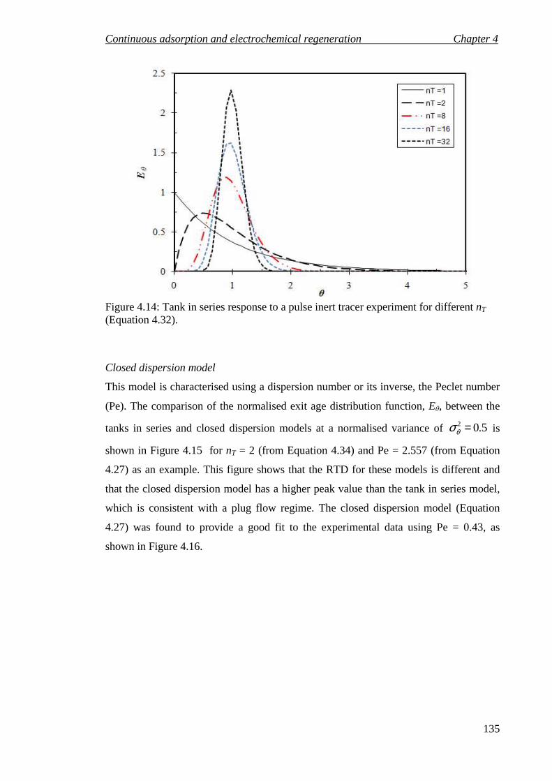
Continuous adsorption and electrochemical regeneration Chapter 4
135
Figure 4.14: Tank in series response to a pulse inert tracer experiment for different nT (Equation 4.32).
Closed dispersion model
This model is characterised using a dispersion number or its inverse, the Peclet number
(Pe). The comparison of the normalised exit age distribution function, Eθ, between the
tanks in series and closed dispersion models at a normalised variance of 5.02 =θσ is
shown in Figure 4.15 for nT = 2 (from Equation 4.34) and Pe = 2.557 (from Equation
4.27) as an example. This figure shows that the RTD for these models is different and
that the closed dispersion model has a higher peak value than the tank in series model,
which is consistent with a plug flow regime. The closed dispersion model (Equation
4.27) was found to provide a good fit to the experimental data using Pe = 0.43, as
shown in Figure 4.16.

Continuous adsorption and electrochemical regeneration Chapter 4
136
Figure 4.15: Comparison between the tanks in series and closed dispersion models at
dimensionless variance 5.02 =θσ corresponding to nT =2 and Pe = 2.557.
Figure 4.16: Comparison of the closed dispersion model (Equation 4.27 fitted to the experimental data with Pe = 0.43 at dimensionless variance 87.02 =θσ ) with the
measured exit age distribution for the small continuous treatment process.
In summary, the behaviour of the continuous treatment process is similar to that of a
single CSTR and the methods of moments (mean residence time and variance) were
used to characterise the RTD. Although other models were able to fit the experimental
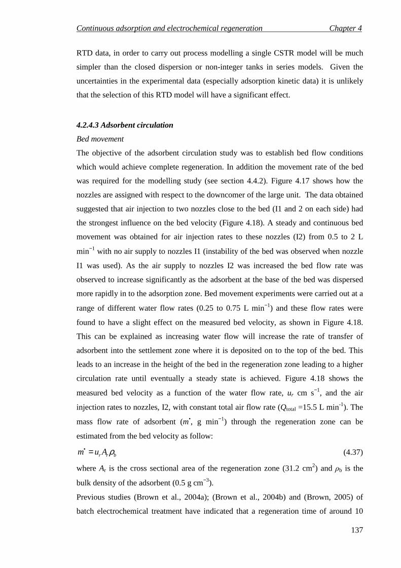
Continuous adsorption and electrochemical regeneration Chapter 4
137
RTD data, in order to carry out process modelling a single CSTR model will be much
simpler than the closed dispersion or non-integer tanks in series models. Given the
uncertainties in the experimental data (especially adsorption kinetic data) it is unlikely
that the selection of this RTD model will have a significant effect.
4.2.4.3 Adsorbent circulation
Bed movement
The objective of the adsorbent circulation study was to establish bed flow conditions
which would achieve complete regeneration. In addition the movement rate of the bed
was required for the modelling study (see section 4.4.2). Figure 4.17 shows how the
nozzles are assigned with respect to the downcomer of the large unit. The data obtained
suggested that air injection to two nozzles close to the bed (I1 and 2 on each side) had
the strongest influence on the bed velocity (Figure 4.18). A steady and continuous bed
movement was obtained for air injection rates to these nozzles (I2) from 0.5 to 2 L
min−1 with no air supply to nozzles I1 (instability of the bed was observed when nozzle
I1 was used). As the air supply to nozzles I2 was increased the bed flow rate was
observed to increase significantly as the adsorbent at the base of the bed was dispersed
more rapidly in to the adsorption zone. Bed movement experiments were carried out at a
range of different water flow rates (0.25 to 0.75 L min−1) and these flow rates were
found to have a slight effect on the measured bed velocity, as shown in Figure 4.18.
This can be explained as increasing water flow will increase the rate of transfer of
adsorbent into the settlement zone where it is deposited on to the top of the bed. This
leads to an increase in the height of the bed in the regeneration zone leading to a higher
circulation rate until eventually a steady state is achieved. Figure 4.18 shows the
measured bed velocity as a function of the water flow rate, ur cm s−1, and the air
injection rates to nozzles, I2, with constant total air flow rate (Qtotal =15.5 L min-1). The
mass flow rate of adsorbent (m•, g min−1) through the regeneration zone can be
estimated from the bed velocity as follow:
brr Aum ρ=• (4.37)
where Ar is the cross sectional area of the regeneration zone (31.2 cm2) and ρb is the
bulk density of the adsorbent (0.5 g cm−3).
Previous studies (Brown et al., 2004a); (Brown et al., 2004b) and (Brown, 2005) of
batch electrochemical treatment have indicated that a regeneration time of around 10
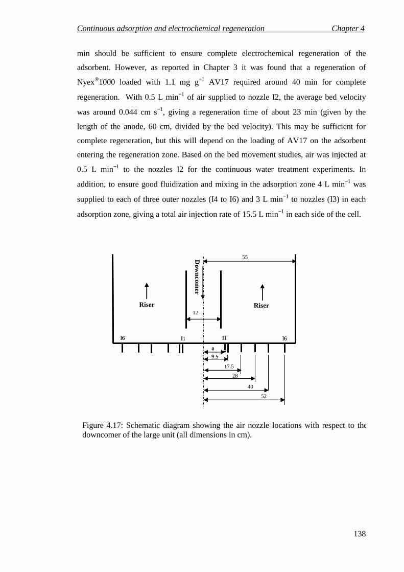
Continuous adsorption and electrochemical regeneration Chapter 4
138
min should be sufficient to ensure complete electrochemical regeneration of the
adsorbent. However, as reported in Chapter 3 it was found that a regeneration of
Nyex®1000 loaded with 1.1 mg g−1 AV17 required around 40 min for complete
regeneration. With 0.5 L min−1 of air supplied to nozzle I2, the average bed velocity
was around 0.044 cm s−1, giving a regeneration time of about 23 min (given by the
length of the anode, 60 cm, divided by the bed velocity). This may be sufficient for
complete regeneration, but this will depend on the loading of AV17 on the adsorbent
entering the regeneration zone. Based on the bed movement studies, air was injected at
0.5 L min−1 to the nozzles I2 for the continuous water treatment experiments. In
addition, to ensure good fluidization and mixing in the adsorption zone 4 L min−1 was
supplied to each of three outer nozzles (I4 to I6) and 3 L min−1 to nozzles (I3) in each
adsorption zone, giving a total air injection rate of 15.5 L min−1 in each side of the cell.
55
17.5
Figure 4.17: Schematic diagram showing the air nozzle locations with respect to the downcomer of the large unit (all dimensions in cm).
Riser
52
40
28
Riser 12
Dow
ncomer
I6 I6 I1 I1
8 9.5
I6 I6 I1 I1
8 9.5

Continuous adsorption and electrochemical regeneration Chapter 4
139
Figure 4.18: Effect of the air injection rate to nozzle I2 on the bed velocity for a total air injection rate of 15.5 L min-1 in each side under different air configuration and water flow rate. The bed velocity was taken from the average of three measurements and the error bars show the standard deviation of the three measurements in each case.
Similar results were also obtained for the small unit, and these results have been
published elsewhere (Mohammed et al. 2011, see Appendix F published paper). Figure
4.19 shows the nozzles location with respect to the downcomer of the small unit, which
were similar to those in the large unit.
Figure 4.19: Schematic diagram showing the air nozzle locations with respect to the downcomer of the small unit (all dimensions in cm).
7.5
13.5
9
10.5
12
15
16.5
17.5
Riser Riser
I7 I1 I7 I1
12
Dow
ncomer
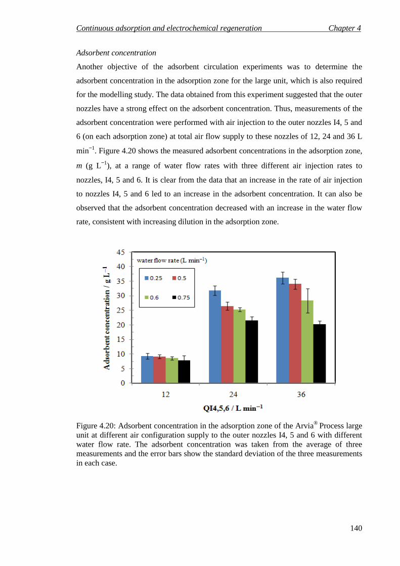
Continuous adsorption and electrochemical regeneration Chapter 4
140
Adsorbent concentration
Another objective of the adsorbent circulation experiments was to determine the
adsorbent concentration in the adsorption zone for the large unit, which is also required
for the modelling study. The data obtained from this experiment suggested that the outer
nozzles have a strong effect on the adsorbent concentration. Thus, measurements of the
adsorbent concentration were performed with air injection to the outer nozzles I4, 5 and
6 (on each adsorption zone) at total air flow supply to these nozzles of 12, 24 and 36 L
min−1. Figure 4.20 shows the measured adsorbent concentrations in the adsorption zone,
m (g L−1), at a range of water flow rates with three different air injection rates to
nozzles, I4, 5 and 6. It is clear from the data that an increase in the rate of air injection
to nozzles I4, 5 and 6 led to an increase in the adsorbent concentration. It can also be
observed that the adsorbent concentration decreased with an increase in the water flow
rate, consistent with increasing dilution in the adsorption zone.
Figure 4.20: Adsorbent concentration in the adsorption zone of the Arvia® Process large unit at different air configuration supply to the outer nozzles I4, 5 and 6 with different water flow rate. The adsorbent concentration was taken from the average of three measurements and the error bars show the standard deviation of the three measurements in each case.

Continuous adsorption and electrochemical regeneration Chapter 4
141
For the small unit, unfortunately it was not possible to accurately sample the solid
−liquid mixture in the adsorption zone in order to determine the adsorbent concentration
due to the relatively narrow width of the adsorption zone.

Continuous adsorption and electrochemical regeneration Chapter 4
142
4.3 Process performance
4.3.1 Introduction
Air lift circulating reactors have been applied widely in continuous wastewater
treatment. Previous studies (Filipkowska and Waraksa, 2008); (Filipkowska, 2004) have
demonstrated the feasibility of an airlift adsorber for dye removal.
In this thesis section the results of the first detailed study of the performance of a
process for treatment of water by continuous adsorption and electrochemical
regeneration occurring in the same device, using a circulating adsorption system are
discussed.
4.3.2 Methodology for continuous water treatment
4.3.2.1 Adsorption and electrochemical regeneration
Continuous water treatment consisting of adsorption and electrochemical regeneration
was carried out to study the performance of AV17 removal on Nyex®1000. The
experiments were carried out using the large reactor and the experimental setup is
shown schematically in Figure 4.21. A solution of AV17 (containing only the dye
dissolved in clean water) with a concentration in the range 80−153 mg L−1 was fed to
the reactor with a flow rate in the range 0.25−0.75 L min−1 in order to demonstrate
continuous removal of AV17. To start up the reactor it was necessary to build up a bed
of adsorbent in the regeneration zone. A feed tank of clean water was used to fill the
reactor before start up. Air was fed to the outer nozzle (I4, 5 and 6) so that the adsorbent
was circulated while no air was fed to the injection points close to the bed (I1 and 2 in
Figure 4.7a). When the bed had been formed in the cell, air was supplied to the I2
injection points close to the bed to enable bed movement. In all cases the total air
injection rate was 31 L min−1 (15.5 L min−1 on each side of the cell). The rate of air
injection to each of the nozzles was 4 L min−1 for I6 to I4, 3 L min−1 for I3 and 0.5 L
min−1 for the nozzles close the regeneration zone (I2) with no air supply to I1. This set
of air flow rates was used for all adsorption and electrochemical regeneration studies in
the large unit. Once a steady state bed movement was established, a constant current of
5 A (corresponding to a current density of approximately 7 mA cm−2 for the 12 cm by
60 cm electrodes) was applied across the moving bed of adsorbent using a DC power

Continuous adsorption and electrochemical regeneration Chapter 4
143
supply (IPS3620, ISO-TECH, UK). This current density was selected based on batch
studies (see section 3.6.3, Chapter 3) and was sufficient to ensure full regeneration of
the adsorbent as it flowed through the electrochemical cell. The catholyte solution
(acidified 0.3 wt% NaCl solution) was circulated through the cathode compartment
using a peristaltic pump (Masterflex 77410-10, Cole-Parmer Instrument Co.) to provide
good conductivity. When current was applied, hydrogen was generated at the cathode
which was entrained with the circulated catholyte. Typical cell voltages of 5–7 V were
obtained during operation. At the start of each experiment the feed solution was
switched from clean water to dye solution, which was supplied at a steady flow rate to
the adsorber. Samples were taken from the out flow at regular intervals for 7 hours or
until the outlet concentration reached a steady state value. Samples were analysed for
AV17 using UV/vis spectroscopy (see section 3.5.1.2, Chapter 3). A similar
methodology was used for the small unit (shown in Figure 4.9) with feed concentrations
in the range 11–110 mg L−1 and feed flow rates in the range 0.24–0.6 L min−1. Details
of the methodology used for the small unit have been published elsewhere (Mohammed
et al. 2011, see Appendix F published paper).

Continuous adsorption and electrochemical regeneration Chapter 4
144
S
Peristaltic pump
Catholyte solution
Tank
Single cell continuous adsorption and regeneration system
AV17 Storage Tank
Water Storage Tank
Peristaltic pump
Drain Valve
Air Air
Figure 4.21: Schematic diagram of the experimental set up for continuous water treatment using the large unit.
4.3.2.2 Adsorption with no regeneration
In order to demonstrate the effect of electrochemical regeneration, experiments were
first carried out with no current supplied to the electrodes. The experiment was
performed with the large unit as described above in section 4.3.2.1, but with zero
current and a feed AV17 concentration of 107 mg L−1 and a feed flow rate of 0.75 L
min−1.

Continuous adsorption and electrochemical regeneration Chapter 4
145
4.3.2.3 Process behaviour in the absence of the adsorbent
In addition to the RTD studies carried out on the small unit, a dilution effect experiment
was carried out in the Arvia® large unit process to confirm that the behaviour of the
large unit was similar to that of a well mixed stirred tank. The adsorber was started up
using clean water with no adsorbent in the reactor. Once the reactor was filled with
water, air was fed to the nozzles (I6 to I2 on each side) with total air flow rate 12 L
min−1. The feed was switched from clean water to a solution of AV17 (27 mg L−1) with
a flow rate 0.75 L min−1. Samples were taken for AV17 analysis from the outlet flow
every 5 minutes for the first two hours and then every 10 minutes until the outlet
concentration approached the initial feed concentration.
4.3.3 Results and discussion 4.3.3.1 Process behaviour in the absence of the adsorbent
In order to demonstrate the reactor residence time distribution characteristics, dye was
injected in the form of a step input to the reactor (large unit) and the response of this
injection are shown in Figure 4.22 in terms of the outlet concentration (Cout, mg L−1)
measurement as a function of time. The theoretical mean residence time, which is equal
to the total volume of the cell divided by volumetric flow rate, was found to be 58 min,
based on a total reactor volume of 43.5 L and a volumetric flow rate is 0.75L min−1. The
outlet steady concentration of AV17 approaches the inlet concentration of around 27 mg
L−1 after about 200 min of operation. Considering the reactor as a single CSTR, the
dynamic mass balance for the AV17 adsorbate with the reactor initially containing only
water (with no adsorbent and no adsorbate) gives Equation (4.38).
)1(inoutτteCC −−= (4.38)
The CSTR-like behaviour is demonstrated for this large unit as shown in Figure 4.22.
The results show that the predicted behaviour of the outlet concentration (Equation
4.38) are in good agreement with experimental data, which indicate the performance of
the large unit is also like a single CSTR.

Continuous adsorption and electrochemical regeneration Chapter 4
146
Figure 4.22: Reactor large unit response to a step input of AV17 in the absence of adsorbent, where the inlet concentration of AV17 was increased from zero to 27 mg L−1 at t = 0, with a feed flow rate of 0.75 L min−1.

Continuous adsorption and electrochemical regeneration Chapter 4
147
4.3.3.2 Adsorption with no regeneration
The performance of the continuous water treatment for adsorption of AV17 onto
Nyex®1000 with no regeneration (no current applied to the electrochemical cell) was
studied in the large unit for a feed concentration of 107 mg L−1 and a flow rate 0.75 L
min−1. The concentration at the exit was measured until a steady state was obtained as
shown in Figure 4.23. The steady state concentration was found to approach the inlet
concentration after around 250 min of operation, which corresponded to conditions
where the adsorbent had become fully saturated with dye. The final maximum loading
of AV17 dye on the adsorbent (qmx, mg g−1) was estimated based on a material balance
assuming that all of the adsorbent in the system reached the same loading qmx, using a
numerical integration of the Cout:
out
0
outinmx )( CM
VdtCC
M
t
−−= ∫ (4.39)
where M is the total mass of adsorbent in the unit. Using Equation (4.39), the loading
after 400 min was found to be around 0.95 mg g−1, which is consistent with the
equilibrium isotherm capacity, kL.
The loading on the adsorbent leaving the adsorption zone (qout, mg g−1) can be estimated
based on the outlet measured concentration, using an overall material balance for the
AV17. Assuming the adsorption zone behaves as a CSTR and so that the concentration
of AV17 and the average loading on the adsorbent in the adsorption zone are equal to
the loading and concentration leaving the adsorption zone (Cout and qout respectively):
dt
dqmV
dt
dCVqmQCqmQC outout
outoutinin +=+−+ •• )()( (4.40)
where qin is the loading on the adsorbent entering the adsorption zone, m• is the mass
flow rate (g min−1) of adsorbent through the regeneration zone and m is the
concentration of adsorbent in the adsorption zone (g L−1).
Rearrangement Equation (4.40), gives:
dt
dC
mqq
mV
mCC
mV
Q
dt
dq outoutinoutin
out 1)()( −−+−=
•
(4.41)
Assuming plug flow of the adsorbent through the regeneration zone with a residence
time of N/m• (where N is the total mass of adsorbent in the regeneration zone, g) we
have:

Continuous adsorption and electrochemical regeneration Chapter 4
148
for t = 0 to t = N / m•, qin = 0 (4.42)
for t > N / m•, qin,exp = qout(t-N/m•) (4.43)
The last term in Equation (4.41), dCout/dt can be estimated from the experimental data.
Solving Equation (4.41) by a numerical method (it was necessary to use Euler
integration rather than Runge-Kutta because of the complex time delay behaviour of qin
and qout) using a MATLAB program with initial conditions Cout(0) = 0 and qout(0) = 0
(the MATLAB program can be found in Appendix D), gives the estimated loading of
dye on the adsorbent leaving the adsorption zone under flow conditions for adsorption
only with bed circulation but no regeneration. The results obtained are plotted in Figure
4.24, where the value of m•=53 g min−1 (from Equation 4.37 and Figure 4.18) and m=20
g L−1 (from Figure 4.20). The adsorbent loading rose rapidly and approached a steady
value of around 0.95 mg g−1 after only 100 to 150 min.
Figure 4.23: Reactor response for adsorption of AV17 onto Nyex®1000 with no regeneration in the Arvia® process large unit.

Continuous adsorption and electrochemical regeneration Chapter 4
149
Figure 4.24: Estimated actual loading from experimental data for AV17 on the adsorbent in the adsorption zone. The loading was calculated from the concentration data shown in Figure 4.23 using a numerical integration of Equation 4.41.

Continuous adsorption and electrochemical regeneration Chapter 4
150
4.3.3.3 Adsorption with electrochemical regeneration A range of inlet concentrations and flow rates were studied to determine the
performance of the treatment process for adsorption with regeneration. The
concentration of AV17 at the exit was monitored until a steady state was obtained. In
order to compare the response of the reactor to the feed flow rate and concentration, the
normalised exit concentration (Cout / Cin) was plotted versus time as shown in Figure
4.25 and Figure 4.26, respectively. The experimental results show that with increasing
flow rate or inlet concentration, the steady state concentration at the outlet increased.
This corresponds to a decrease in the percentage of AV17 removed (see Table 4.2),
calculated as:
%100.in
outin
C
CCR
−= (4.44)
The time required to reach steady state varied from 150 to 270 min, and depended on
the feed flow rate and concentration as shown in Table 4.2. The shortest operating time
required to reach steady state was observed for high feed flow rate and concentration
due to the higher rate that dye (mg min−1) was fed to the system under these conditions.
Table 4.2: Percentage removal of AV17 at different flow rate and initial concentration for adsorption and regeneration process.
Cin (mg L−1) Q (L min−1) % AV17 Removed Time required to reach
steady state (min)
99 0.75 44 150
99 0.5 54 210
99 0.25 91 250
153 0.6 30 240
140 0.6 34 250
80 0.6 53 270

Continuous adsorption and electrochemical regeneration Chapter 4
151
Figure 4.25: Reactor performance for adsorption and regeneration at various influent flow rates in the Arvia® large unit.
Figure 4.26: Reactor performance for adsorption and regeneration at different initial concentration in the Arvia® large unit.

Continuous adsorption and electrochemical regeneration Chapter 4
152
As before, the loading of AV17 on the adsorbent leaving the adsorption zone (qout, mg
g−1) can be estimated from the measured outlet AV17 concentration (Cout) using an
overall material balance for the AV17. The equations obtained are as before (Equations
4.40 and 4.41) but in this case qin = 0, assuming complete regeneration of the adsorbent
in the adsorption zone:
)()(dt
dqmV
dt
dCVqmQCQC outout
outoutin +=+− • (4.45)
Rearrangement of Equation (4.45), gives:
dt
dC
mq
mV
mCC
mV
Q
dt
dq outoutoutin
out 1)( −−−=
•
(4.46)
As before, the last term in Equation (4.46), dCout/dt can be estimated from the
experimental data. Equation (4.46) was integrated numerically (fourth order Runge
Kutta integration) using a MATLAB program with initial conditions Cout(0) = 0 and
qout(0) = 0 (the MATLAB program can be found in Appendix D), to estimate the
loading of dye on the adsorbent leaving the adsorption zone.
The calculated adsorption loading of AV17 on the adsorbent leaving the adsorption
zone (qout, mg g−1) under continuous flow for adsorption with regeneration was
determined under for each set of experimental conditions, using the parameter values
shown in Table 4.3, where the volume of the adsorption zone was equal to 36 L.
Table 4.3: Values of the parameters m• and m used to calculate qout from the outlet experimental concentration (Cout).
Cin (mg L−1) Q (L min−1) m• (g min−1)
Figure 4.18 and (Eq. 4.37)
m (g L−1)
(Figure 4.20)
99 0.75 50 20
99 0.5 41 27
99 0.25 40.5 30
153 0.6 42 25
140 0.6 42 25
80 0.6 42 25
With increasing flow rate, the loading of AV17 on the adsorbent in the adsorption zone
was found to increase slightly (see Figure 4.27) due to an increase in the rate of

Continuous adsorption and electrochemical regeneration Chapter 4
153
contaminant removal (i.e. the mg of contaminant removed per min) (although the
percentage removal decreases as shown in Table 4.2). Similarly, with a higher feed
concentration of AV17, it was found that the loading of dye on the adsorbent increased
(Figure 4.28) again due to an increase in the rate of adsorption. This performance is
similar to that of a chemical reaction in a CSTR; typically with increasing flow rate the
conversion decreases and the average rate of reaction increases.
The observed adsorbent loadings entering the regeneration zone are around 0.6 mg g−1,
significantly lower than the maximum loadings used in the batch studies. With this
loading the time required for complete regeneration can be estimated to be around 22
min, suggesting that the residence time in the regeneration zone should be sufficient for
complete regeneration.
Figure 4.27: Estimated loading of AV17 on the adsorbent in the adsorption zone for various values of the feed flow rate. The loading was calculated from the concentration data shown in Figure 4.25 using a numerical integration of Equation 4.46.

Continuous adsorption and electrochemical regeneration Chapter 4
154
Figure 4.28: Estimated loading of AV17 on the adsorbent in the adsorption zone for various values of the feed concentration. The loading was calculated from the concentration data shown in Figure 4.26 using a numerical integration of Equation 4.46.
As mentioned in the methodology section, the total air injection rate was 31 L min−1
(15.5 L min−1 on each side of the cell). The rate of air injection to each of the nozzles
was 4 L min−1 for I6 to I4 and 3 L min−1 for I3 whereas it was 0.5 L min−1 for the
nozzles close the regeneration zone (I2) with no air supply to I1. This configuration of
air injection gave a residence time for adsorbent in the regeneration zone in the order of
23 min. Continuous removal of AV17 was achieved with removals of 90% or higher for
inlet concentration of up to 99 mg L−1 (as shown in Table 4.2) at a feed flow rate 0.25 L
min−1. When the feed flow rate Q was increased at a feed concentration of 99 mg L−1
the removal achieved decreased, due to the decreased residence time and the increased
loading on the adsorbent.
The results confirm that regeneration of the adsorbent was being achieved. In the
absence of regeneration (when no current is applied to the electrochemical cell) the
outlet concentration was found to approach the inlet concentration as shown in Figure
4.29. In contrast with a current applied to the regeneration cell, removals of up to 90%
were achieved at steady state. In this thesis the effect of the current density was not
explored and this will be the subject of future work. However, based on batch
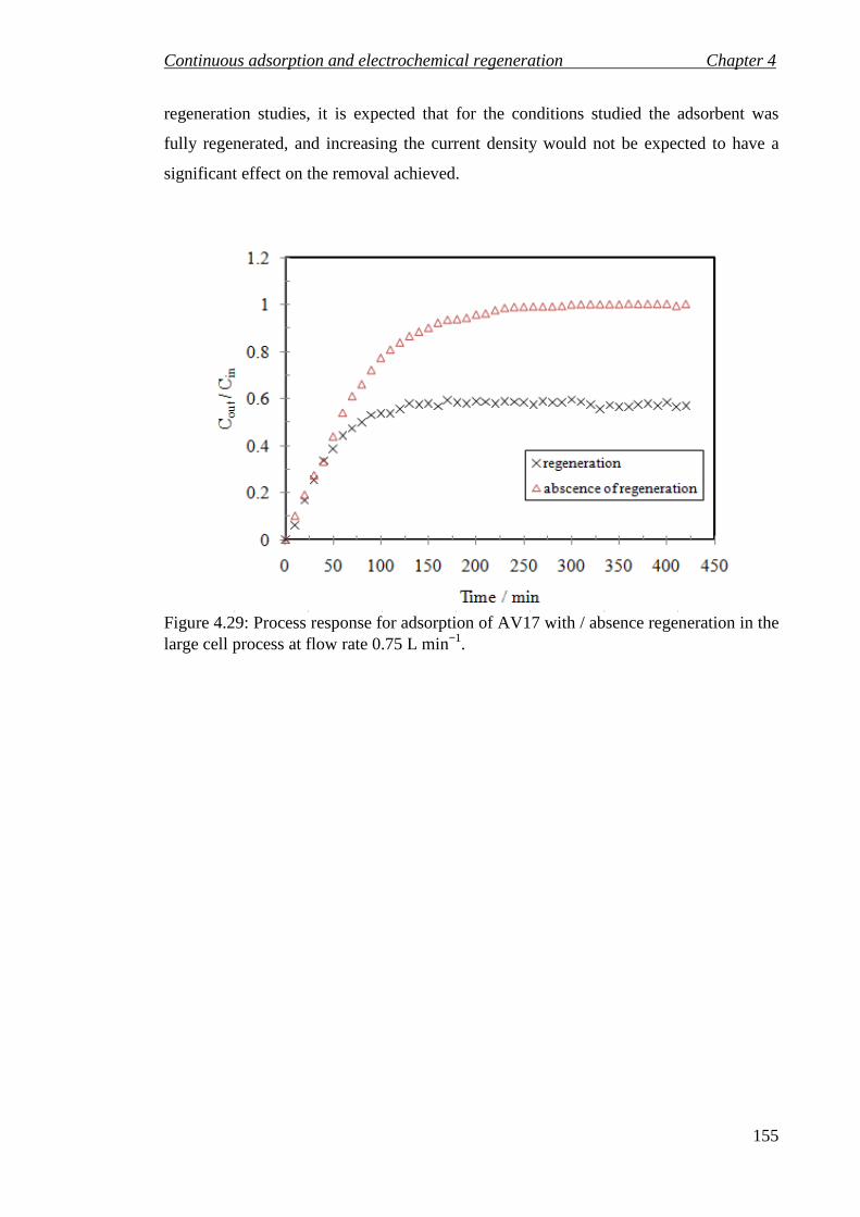
Continuous adsorption and electrochemical regeneration Chapter 4
155
regeneration studies, it is expected that for the conditions studied the adsorbent was
fully regenerated, and increasing the current density would not be expected to have a
significant effect on the removal achieved.
Figure 4.29: Process response for adsorption of AV17 with / absence regeneration in the large cell process at flow rate 0.75 L min−1.

Continuous adsorption and electrochemical regeneration Chapter 4
156
4.4 Process modelling
4.4.1 Introduction
The purpose of any mathematical model is to reduce the effort, scope and magnitude of
laboratory and pilot-scale studies and also to enable the design of large-scale processes
economically and efficiently. Hence, it is necessary to develop mathematical models to
predict/simulate process behaviour and improve process understanding. Many different
mathematical models for adsorption and desorption in a fixed bed process have been
developed (Soos et al., 2000). These previous studies have considered the adsorption
process by applying a mathematical model to an isothermal, fixed bed axial dispersion
design, and to the pore diffusion model for a sorbent particle. However, no studies have
been directed to the modelling of a continuous airlift adsorber for water treatment by
adsorption with continuous regeneration of the adsorbent. In this thesis a numerical
model of the continuous water treatment for adsorption with or without an
electrochemical regeneration process is developed for the first time, using a circulating
adsorbent in an airlift system, so as to predict the exit concentration and the outlet
adsorbent loading from the adsorption zone.
In this section, a discussion is presented of mathematical models of adsorption with
regeneration, and adsorption with no regeneration. For the simulation of adsorption with
regeneration, both transient and steady-state models are considered, whereas for
adsorption with no generation, only the dynamic model is discussed (since in the
absence of regeneration the steady state model is trivial).
4.4.2 Theoretical equations
A numerical model based on the adsorbate mass balance has been used to describe the
continuous adsorption process with or without electrochemical regeneration under
dynamic conditions for continuous water treatment.
4.4.2.1 Process modelling for adsorption with no regeneration
A model has been developed in order to predict the outlet concentration and the
adsorbent loading for a given set of operating conditions. However, the adsorbent
loading occurring during the experiments has been estimated based on an overall mass

Continuous adsorption and electrochemical regeneration Chapter 4
157
balance. In this study the focus is on the adsorption zone, as this is where the water
treatment is carried out. The RTD study indicates that the adsorption zone can be
considered to behave like a CSTR, so that a material balance for the AV17 can be
constructed as shown in Figure 4.30.
Q (L min-1) Cout (mg L-1)
Q (L min-1) Cin (mg L-1)
Adsorption Zone Bed
V (L) m (g L−1)
N (g) m• (g min−1)
qout (mg g−1)
qin (mg g−1)
Figure 4.30: Schematic diagram of the processes occurring in the continuous adsorption with no regeneration adsorber.
The feed flow rate of waste water contaminated with the dye enters the adsorber
continuously at a flow rate Q and a constant dye concentration Cin. The adsorber
initially contains no solute (i.e. clean water) and fresh adsorbent (i.e. with zero loading
of organic dye). Since the adsorption zone is assumed to behave as a CSTR, the
concentration of dye throughout the adsorption zone is assumed to be equal to the outlet
concentration Cout. In addition, the adsorbent loading throughout the adsorption zone
will be assumed to be equal to the average loading of the adsorbent leaving the
adsorption zone qout. In practice the loading of each adsorbent particle will depend on
the length of time it has spent in the adsorption zone. However, consideration of the
effect of the distribution of adsorbent loading will significantly complicate the model.
Given the uncertainty in the experimentally determined kinetic rate constants (discussed
in Chapter 3), it is unlikely that the approximation of uniform adsorbent loading will
significantly effect the results of the model in comparison with experimental data.
An unsteady state mass balance for AV17 dye (the adsorbate) for the liquid phase in the
adsorption zone gives:
Continuous adsorption and electrochemical regeneration Chapter 4
158
Vdt
dCVrQCQC d
outoutin =−− (4.47)
where V is the adsorption zone volume (L) and Cout is the outlet concentration (mg L−1).
Based on the batch experiments (Chapter 3) we assume second order kinetics and a
Langmuir isotherm for the adsorption equilibrium, so the rate of adsorption per unit
volume, rd (mg min−1 L−1) throughout the adsorption zone is given by:
2
outout
out2 1
−
+= q
bC
Cbkmkr L
d (4.48)
where qout is the loading of AV17 on the adsorbent (mg g−1) leaving the adsorption zone
and m is the mass of adsorbent per unit volume of the adsorption zone. Combining
Equations (4.47) and (4.48) we obtain:
2
outout
out2outin
out
1)(
−
+−−= q
bC
CbkmkCC
V
Q
dt
dC L (4.49)
The mass balance for the AV17 dye on the solid phase for the adsorption zone gives:
mVdt
dqVrmqmq d
outoutin =+− •• (4.50)
where qin is the loading of AV17 on the adsorbent (mg g−1) entering the adsorption zone
and m• is the mass flow rate (g min−1) of adsorbent through the regeneration zone
(Equation 4.41). Combining Equations (4.48) and (4.50) we obtain:
2
outout
out2outin
out
1)(
−
++−=
•
qbC
Cbkkqq
mV
m
dt
dq L (4.51)
Although there is no regeneration, initially the system is filled with fresh adsorbent, so
that the adsorbent entering the adsorption zone will have zero loading until all of the
adsorbent initially in the regeneration zone has flowed into the adsorption zone.
Assuming plug flow of the adsorbent through the regeneration zone with a residence
time of N/m• (where N is the total mass of adsorbent (g) in the regeneration zone) we
have:
for t = 0 to t = N/m•, qin = 0 (4.52)
for t > N/m•, qin = qout (t-N/m•) (4.53)
Solving Equations (4.49) and (4.51) by a numerical integration (it was necessary to use
Euler integration rather than Runge-Kutta because of the complex time delay behaviour
of qin and qout) using a MATLAB program at a step size h = 0.001. Tests were carried
out with a range of values of h to ensure that the step size was sufficiently small to
Continuous adsorption and electrochemical regeneration Chapter 4
159
obtain accurate results (see Appendix E), with initial conditions 0)0(out =C and
0)0(out =q , respectively (the MATLAB program can be found in Appendix D), gives
the adsorption dynamic model for the continuous process of adsorption with no
regeneration. This is equivalent to the experimental conditions where no current was
applied described in section 4.3.3.2.
4.4.2.2 Process modelling for adsorption with electrochemical regeneration For the adsorption with regeneration process, a model has been developed in order to
predict the exit concentration (Cout) for a given set of operating conditions. It will be
assumed that the electrochemical cell is operated under conditions which achieve 100%
regeneration of the adsorbent. This assumption is justified based on batch experiments
(Chapter three) and also based on previous studies of batch electrochemical
regeneration of GIC adsorbents (Brown et al., 2004a); (Brown et al., 2004b). Previous
studies have developed models of continuous adsorption processes, e.g. Maji et al.
(2007) and Najm (1996), and in this thesis we modify these to account for the
continuous supply of fresh adsorbent. As previously mentioned, the RTD behaviour of
this adsorber is similar to that of a single CSTR, therefore a material balance for the dye
for the adsorption zone can be constructed as shown in Figure 4.31 for steady state and
dynamic conditions.

Continuous adsorption and electrochemical regeneration Chapter 4
160
Q (L min-1) Cout (mg L-1)
Q (L min-1) Cin (mg L-1)
Adsorption Zone Electrochemical Regeneration Zone
V (L) m (g L−1)
m• (g min−1)
qout (mg g−1)
qin (mg g−1)
m• (g min−1)
Figure 4.31: Schematic diagram of the processes occurring in the continuous adsorption with electrochemical regeneration reactor.
Steady state
At steady state, the outlet concentration has a constant value of Cout and an overall
material balance on AV17 dye for the adsorption zone with a constant inlet
concentration (Cin) gives:
0)()( outoutinin =+−+ •• mqQCmqQC (4.54)
Assuming complete regeneration (qin = 0), Equation (4.54) becomes:
)( outinout CCm
Qq −= • (4.55)
Combining Equations (4.54) and (4.48) we obtain:
2
outinout
out2outin )(
1)(
−−
+=− • CC
m
Q
bC
CbkmVkCCQ L (4.56)
Solving Equation (4.56) numerically using the Solver tool in Microsoft Excel® (see
section 4.4.3.2) we can obtain Cout for a given set of operating conditions (Q, Cin, V, m•
and m) provided the kinetic and isotherm parameters (k2, b and kL) for the adsorbate /
adsorbent system are known.

Continuous adsorption and electrochemical regeneration Chapter 4
161
Dynamic
The dynamic material balance for AV17 for adsorption with regeneration process in the
liquid phase gives the same equation as that for adsorption with no regeneration
(Equation 4.49). However, a mass balance of AV17 in the solid phase for adsorption
with regeneration can be described as follows:
mVdt
dqVrmqmq d
outoutin =+− •• (4.57)
As with the steady state material balance complete regeneration is assumed (qin = 0) and
combining Equations (4.57) and (4.48) we obtain:
2
outout
out2
outout
1
−
++−=
•
qbC
Cbkk
mV
mq
dt
dq L (4.58)
Solving Equations (4.49) and (4.58) by numerical integration (fourth and fifth order
Runge Kutta, “ode45”) using a MATLAB program with initial conditions Cout(0) = 0
and qout(0) = 0 and step size h = 0.001 (see Appendix D, MATLAB program), the
variation of Cout and qout with time can be predicted for a given set of operating
conditions. Tests were carried out with a range of values of h to ensure that the step size
was sufficiently small to obtain accurate results (see Appendix E).
4.4.3 Numerical methodology and implementation
4.4.3.1 Integration of ordinary differential equation
Differential equations are mathematical expressions for an unknown function of one or
more independent variables which relate the values of the function itself and its
derivatives of various orders. Ordinary differential equations (ODEs) and partial
differential equations (PDEs) are commonly used for modelling in mathematics,
engineering and science to illustrate how material quantities vary (Shampine et al.,
2003). Their solutions demonstrate the response of the dependent variables to the
independent variables.
The differential equations developed in section 4.4.2 are ordinary differential equations
in which all dependent variables (the exit concentration Cout and the outlet adsorption
capacity qout) depend on a single independent variable (time, t). In this section the two
most widely used methods of numerically integrating ordinary differential equations
(ODEs), Euler’s method and Runge Kutta integration, which have been used in this
study, are described.

Continuous adsorption and electrochemical regeneration Chapter 4
162
Euler’s method
Euler’s method is the simplest numerical integration method. It is widely for solving
ODEs although it has a relatively low accuracy. To obtain accurate results, small step
size (h) must be used (Boyce and DiPrima, 1997). In this study, the forward Euler
method was used to solve the ODEs for the model of adsorption with no regeneration
with step size h = 0.001. Tests were carried out with a range of value of h to ensure that
the step size was sufficiently small to obtain accurate results (see Appendix E). The
ODEs are of the form:
),,( )(outout(n)outout
nn qCtfCdt
dC =′= (4.59)
),,( out(n)out(n)outout qCtgq
dt
dqn=′= (4.60)
with the initial values Cout(0) = 0 and qout(0) = 0. The general Euler approximation for
these equations is (Boyce and DiPrima, 1997):
),,( )(out)(out)(out)1(out nnnnn qCthfCC +=+ (4.61)
),,( )(out)(out)(out)1(out nnnnn qCthgqq +=+ (4.62)
where h is a uniform step between the points t0 to tn, then tn+1 − tn =h, and
)( 1out)1(out ++ ≈ nn tCC
)( 1out)1(out ++ ≈ nn tqq
Runge Kutta integration
This method is one of the most widely used tools for solving ODEs. In this thesis,
fourth and fifth order Runge-Kutta integration (RK4 and 5) was implemented using the
“ode45” built in Matlab routine (as recommended by Dormand and Prince, 1980). This
method has been used to solve the adsorption with regeneration model with a step size h
= 0.001. The first order ODEs to be solved are of the form:
),,( outoutoutout qCtfC
dt
dC =′= (4.63)
),,( outoutoutout qCtgq
dt
dq =′= (4.64)
with the initial values Cout(0) = 0 and qout(0) = 0. The problem is solved by stepping
forward in time from t = 0 with a constant step size h. The Runge Kutta scheme for the
first order ODEs can be written as (Guterman and Nitecki, 1984).

Continuous adsorption and electrochemical regeneration Chapter 4
163
)22(6 4321)(out)1(out FFFFh
CC nn ++++=+ (4.65)
)22(6 4321)(out)1(out GGGGh
qq nn ++++=+ (4.66)
where Cout(n+1) and qout(n+1) are the RK4 approximation of Cout(tn+1) and qout(tn+1),
respectively, and
),,( )(out)(out1 nnn qCtfF = (4.67)
),,( )(out)(out1 nnn qCtgG = (4.68)
)2
1,
2
1,
2
1( 1)(1)(2 hGqhFChtfF noutnoutn +++= (4.69)
)2
1,
2
1,
2
1( 1)(out1)(out2 hGqhFChtgG nnn +++= (4.70)
)2
1,
2
1,
2
1( 2)(out2)(out3 hGqhFChtfF nnn +++= (4.71)
)2
1,
2
1,
2
1( 2)(out2)(out3 hGqhFChtgG nnn +++= (4.72)
),,( 3)(out3)(out4 hGqhFChtfF nnn +++= (4.73)
),,( 3)(out3)(out4 hGqhFChtgG nnn +++= (4.74)
Thus, the value Cout and qout at the next time step (Cout(n+1) and qout(n+1)) are determined
from the values at the current time step, Cout(n) and qout(n), using the product of the step
size (h) and an estimated slope. The slope is a weighted average of slopes (Boyce and
DiPrima, 1997):
• F1, G1 are the slope at the beginning of the interval;
• F2, G2 are the slope at the midpoint of the interval, using the slopes F1 and G1 to
determine the value of Cout and qout at 2htn + using Euler’s method;
• F3, G3 are a second approximation to the slope at the midpoint, but now using
the slopes F2 and G2 to determine the Cout and qout at 2htn + ;
• F4, G4 are the slope at the end of the interval (tn+ h), with the values or Cout and
qout determined using Euler’s method and the slopes F3 and G3.

Continuous adsorption and electrochemical regeneration Chapter 4
164
4.4.3.2 Solution to non-linear equations - Microsoft Excel solver technique
As mentioned and discussed in Chapter 3, the Microsoft Excel spreadsheet software
package includes a numerical optimization add-in called ‘Solver’. The non-linear
Equation (4.56), which is a steady state model for adsorption and electrochemical
regeneration, was solved using Microsoft Excel’s Solver add-in to determine the steady
state outlet concentration. The Solver tool was implemented using a forward derivative
Newton’s method iteration. The target used for this technique was the minimization of
the square error between the right hand side and left hand side of Equation (4.56) (with
a convergence limit of 10−4), which was achieved by adjusting the outlet concentration
Cout (mg L−1) in order to satisfy Equation (4.56).
4.4.4 Modelling validation results and discussion
In this section, the models which have been described in section (4.4.2) are validated by
comparison with the experimental results.
4.4.4.1 Adsorption with no regeneration
The outlet concentration and adsorption capacity (Cout and qout) for the case of
adsorption with no regeneration (i.e. circulating adsorbent but no current applied) can be
predicted by solving Equations (4.49) and (4.51) simultaneously, for a given flow rate
and feed concentration if the values of the parameters V, k2, b, kL, N, m, and m• are
known. These equations have been solved numerically using Euler integration method
using a MATLAB program. The amount of adsorbent inside the bed was estimated to be
N = 1500 g, the initial conditions were Cout(0) = 0 and qout(0) = 0, and the other
parameters used are shown in Table 4.4.
Table 4.4: Values of the parameters used in the model.
Parameter Value Source
V 36 L Volume of adsorption zone
k2 0.41 g mg−1 min−1 Table 3.2
b 0.31 L mg−1 Table 3.4
kL 0.987 mg g−1 Table 3.4
m Varies dependent on Q (g L−1) Table 4.3
m• Varies dependent on Q ( g min−1) Table 4.3
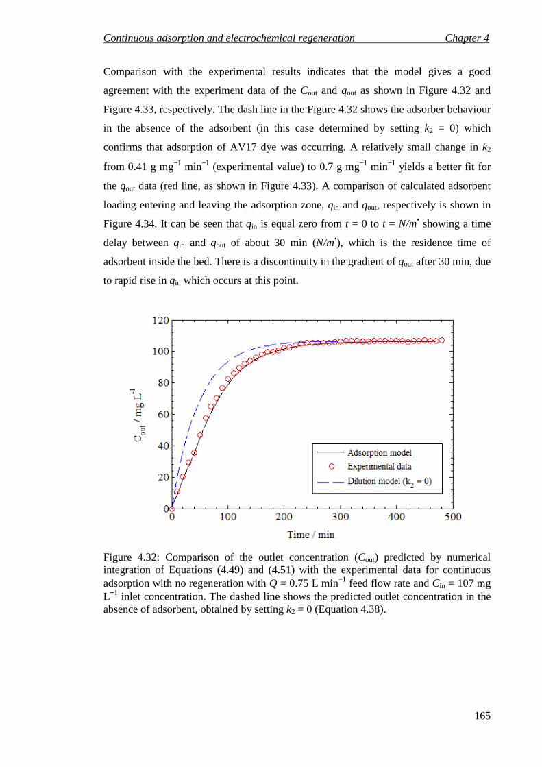
Continuous adsorption and electrochemical regeneration Chapter 4
165
Comparison with the experimental results indicates that the model gives a good
agreement with the experiment data of the Cout and qout as shown in Figure 4.32 and
Figure 4.33, respectively. The dash line in the Figure 4.32 shows the adsorber behaviour
in the absence of the adsorbent (in this case determined by setting k2 = 0) which
confirms that adsorption of AV17 dye was occurring. A relatively small change in k2
from 0.41 g mg−1 min−1 (experimental value) to 0.7 g mg−1 min−1 yields a better fit for
the qout data (red line, as shown in Figure 4.33). A comparison of calculated adsorbent
loading entering and leaving the adsorption zone, qin and qout, respectively is shown in
Figure 4.34. It can be seen that qin is equal zero from t = 0 to t = N/m• showing a time
delay between qin and qout of about 30 min (N/m•), which is the residence time of
adsorbent inside the bed. There is a discontinuity in the gradient of qout after 30 min, due
to rapid rise in qin which occurs at this point.
Figure 4.32: Comparison of the outlet concentration (Cout) predicted by numerical integration of Equations (4.49) and (4.51) with the experimental data for continuous adsorption with no regeneration with Q = 0.75 L min−1 feed flow rate and Cin = 107 mg L−1 inlet concentration. The dashed line shows the predicted outlet concentration in the absence of adsorbent, obtained by setting k2 = 0 (Equation 4.38).

Continuous adsorption and electrochemical regeneration Chapter 4
166
Figure 4.33: Comparison of the outlet adsorbent loading (qout) predicted by numerical integration of Equations (4.49) and (4.51) with the values estimated from the experimental data for continuous adsorption with no regeneration with Q = 0.75 L min−1 feed flow rate and Cin = 107 mg L−1. The red line shows the best fit at an adjusted k2 value of 0.7 g mg−1 min−1.
Figure 4.34: Comparison of the loading of the adsorbent leaving the adsorption zone (qout) calculated by numerical integration of Equations (4.49) and (4.51) and the loading of the adsorbent entering the adsorption zone (qin) determined from Equations (4.52) and (4.53), for the case of continuous adsorption with no regeneration.

Continuous adsorption and electrochemical regeneration Chapter 4
167
In order to illustrate the importance of continuous regeneration for this system, the
effect of the key parameters (Q, Cin and V) on the performance of the process in the
absence of regeneration was studied. In order to consider the feed flow rate Q using the
model, it is necessary to estimate the adsorbent circulation rate and concentration (m•
and m). The adsorbent circulation rate was not found to be strongly dependent on the
feed flow rate so for the purposes of this study a constant adsorbent circulation rate of
m•=40.5 g min−1 was assumed. The adsorbent concentration was measured
experimentally only for a limited range of feed flow rate of 0.25–0.75 L min−1. In order
to investigate the predicted trends for a wider range of feed flow rates, as a first
approximation it was assumed that the adsorbent travelled with the no slip velocity, so
the adsorbent concentration was estimated from:
Q
mm
•
= (4.75)
Although the adsorbent might be expected to travel at a lower velocity than the
contaminated water as it has a high density, it may also be attracted to the surface of the
air bubble rising though the contaminated water. However, there was a significant
difference between the measured concentrations of adsorbent in the adsorption zone
with those predicted using Equation (4.75), as shown in Table 4.5. Therefore, measured
adsorbent concentrations have been plotted against the water feed flow rates (Figure
4.35), and the adsorbent concentration was estimated assuming the linear relationship:
6.3525.19 +−= Qm (4.76)
Table 4.5: Values of parameters for the measured and predicted concentrations in the adsorption zone at different feed flow rate.
Q
(L min-1)
m•
(g min−1)
m measured
(g L-1)
m predicted from Eq.(4.75)
(g L-1)
0.75 50 20 66.66
0.6 42 25 70
0.5 41 27 82
0.25 40.5 30 162

Continuous adsorption and electrochemical regeneration Chapter 4
168
Figure 4.35: Measured concentrations of adsorbent in the adsorption zone of the large unit at a range of feed flow rate. The line shows the linear relationship (Equation 4.76) fitted to the data by linear regression.
For a feed concentration (Cin) of 107 mg L−1, Equations 4.49 and 4.51 were integrated
for a range of feed flow rate using the parameters of the isotherm and kinetics constants
from Table 4.4 and the adsorbent concentration from Equation (4.76). The outlet
concentration Cout obtained at the end of 5 hours of operation is plotted against feed
flow rate in Figure 4.36. At low flow rates it was found that the percentage removal was
high (since Cout was much less than Cin) since the rate of addition of contaminant to the
system is low and after 300 min the adsorbent has not had time to become saturated. As
the flow rate increase Cout and qout increase until Cout approaches Cin (i.e. no removal, as
shown in Figure 4.37).
The point at which the adsorbent will become saturated can be estimated by comparing
the amount of contaminant added during the first 300 min of operation with the total
adsorption capacity available. Thus the adsorbent would be expected to become
saturated when:
MqtQC ein > (4.77)
where qe is the adsorbent loading at equilibrium with the feed concentration Ce and M is
the total amount of adsorbent in the system. For Cin = 107 mg L−1 we can determine qe =
0.95 mg g−1 from the isotherm data, and we have t = 300 min, M = 4000 g. Substituting

Continuous adsorption and electrochemical regeneration Chapter 4
169
these values into Equation (4.77), we would expect the percentage removal to decreases
when Q > 0.12 L min−1, which is reasonably consistent with the results shown in Figure
4.37.
Figure 4.36: Variation of the calculated values of Cout and qout (determined by numerical integration of Equations 4.49 and 4.51) after 300 min of continuous adsorption with no regneration for a range of feed flow rates Q at a feed concentration of 107 mg L−1.
Figure 4.37: Variation of the percentage removal with feed flow rate based on the data shown in Figure 4.36.

Continuous adsorption and electrochemical regeneration Chapter 4
170
Similarly, with increasing inlet concentration Cin (at constant feed flow rate Q as shown
in Figure 4.38), the outlet concentration Cout increased and approaches Cin for Cin higher
than ~100 mg L−1 as the adsorbent became saturated.
Figure 4.38: Variation of the calculated values of Cout and qout (determined by numerical integration of Equations 4.49 and 4.51) after 300 min of continuous adsorption with no regneration for a range of feed concentration Cin and at a feed flow rate of 0.75 L min−1.
With increasing adsorber volume (V), the breakthrough of Cout is slightly slower due to
the Q / V term in the differential equation (Equation 4.49). Hence Cout decreases slightly
for a feed flow rate of 0.75 L min−1 and inlet concentration of 107 mg L−1 as shown in
Figure 4.39 indicating that after 300 min conditions are moving away from steady state
as V is increased. The adsorbent was found to become saturated for reactor volumes
larger than 35 L .

Continuous adsorption and electrochemical regeneration Chapter 4
171
Figure 4.39: Variation of the calculated values of Cout and qout (determined by numerical integration of Equations 4.49 and 4.51) after 300 min of continuous adsorption with no regneration for a feed flow rate of 0.75 L min−1 and inlet concentration of 107 mg L−1.
4.4.4.2 Adsorption with electrochemical regeneration Steady state model
For a given feed flow rate (Q) and inlet concentration (Cin), the outlet concentration Cout
can be determined by solving Equation (4.56) numerically if the values of V, k2, b, kL,
m, and m• are known. The values of all of these parameters (shown in Table 4.4) have
been measured and applied to solve Equation (4.56) using the Solver tool in Microsoft
Excel® as discussed in section (4.4.3.2). It was found that for a given set of conditions
two real solutions could be obtained, but the lower value of Cout obtained was unfeasible
as in this case the term inside the square brackets was negative (i.e. qe < qout). A
comparison of the percentage removal obtained based on the value of Cout predicted
from Equation (4.56) with that obtained from the experimentally measured values of
Cout (using the larger process unit) for a range of operating conditions is shown in
Figure 4.40. The results indicate that the model gives a good prediction (within 2.5 %)
of the percentage removal in all cases for the range of conditions studied. Similar results
were also obtained for the small unit, and these results are shown in Figure 4.41 which
shows good agreement with the model predictions (within 4.6%). This model was

Continuous adsorption and electrochemical regeneration Chapter 4
172
solved using the parameter values shown elsewhere (Mohammed et al., 2011, see
Appendix F, published paper).
Figure 4.40: Comparison of the percentage removal predicted from the numerical solution to Equation (4.56) with the experimental values obtained for continuous adsorption and electrochemical regeneration process in the large unit. A range of inlet concentrations of AV17 and solution flow rates were used, as discussed in section 4.3.3.3. The larger open symbols indicate the experimental data, while the smaller filled symbols show the predicted removal based on Equation (4.56).
Figure 4.41: Comparison of the percentage removal predicted from the numerical solution to Equation (4.56) with the experimental values obtained for continuous adsorption and electrochemical regeneration process in the small unit. A range of inlet concentrations of AV17 and solution flow rates were used, as described in Mohammed et al. (2011), see Appendix F. The larger open symbols indicate the experimental data, while the smaller filled symbols show the predicted removal based on Equation (4.56).
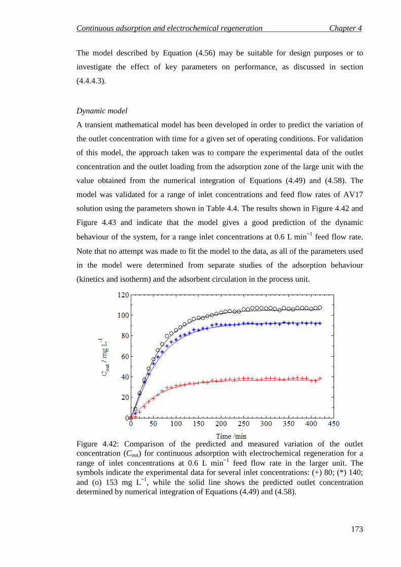
Continuous adsorption and electrochemical regeneration Chapter 4
173
The model described by Equation (4.56) may be suitable for design purposes or to
investigate the effect of key parameters on performance, as discussed in section
(4.4.4.3).
Dynamic model
A transient mathematical model has been developed in order to predict the variation of
the outlet concentration with time for a given set of operating conditions. For validation
of this model, the approach taken was to compare the experimental data of the outlet
concentration and the outlet loading from the adsorption zone of the large unit with the
value obtained from the numerical integration of Equations (4.49) and (4.58). The
model was validated for a range of inlet concentrations and feed flow rates of AV17
solution using the parameters shown in Table 4.4. The results shown in Figure 4.42 and
Figure 4.43 and indicate that the model gives a good prediction of the dynamic
behaviour of the system, for a range inlet concentrations at 0.6 L min−1 feed flow rate.
Note that no attempt was made to fit the model to the data, as all of the parameters used
in the model were determined from separate studies of the adsorption behaviour
(kinetics and isotherm) and the adsorbent circulation in the process unit.
Figure 4.42: Comparison of the predicted and measured variation of the outlet concentration (Cout) for continuous adsorption with electrochemical regeneration for a range of inlet concentrations at 0.6 L min−1 feed flow rate in the larger unit. The symbols indicate the experimental data for several inlet concentrations: (+) 80; (*) 140; and (o) 153 mg L−1, while the solid line shows the predicted outlet concentration determined by numerical integration of Equations (4.49) and (4.58).
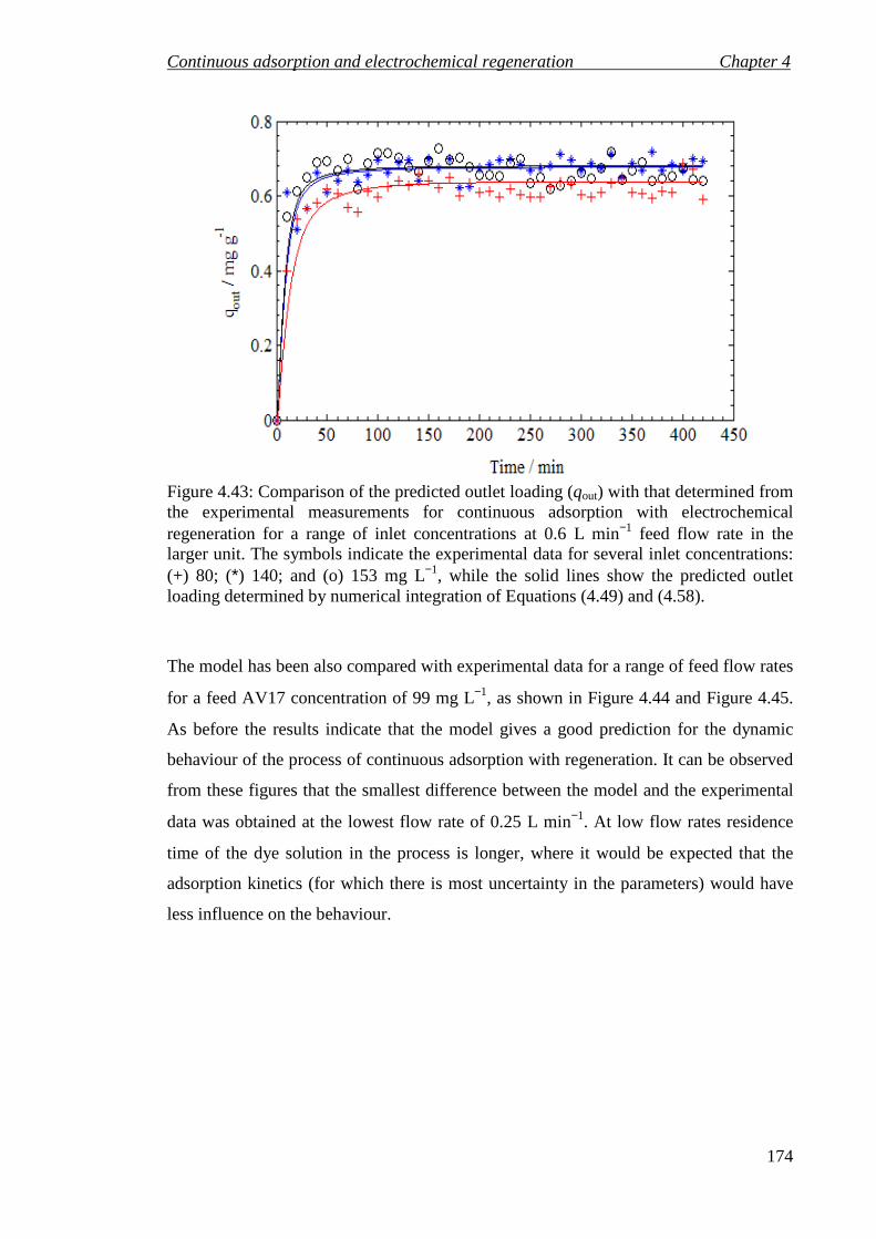
Continuous adsorption and electrochemical regeneration Chapter 4
174
Figure 4.43: Comparison of the predicted outlet loading (qout) with that determined from the experimental measurements for continuous adsorption with electrochemical regeneration for a range of inlet concentrations at 0.6 L min−1 feed flow rate in the larger unit. The symbols indicate the experimental data for several inlet concentrations: (+) 80; (*) 140; and (o) 153 mg L−1, while the solid lines show the predicted outlet loading determined by numerical integration of Equations (4.49) and (4.58).
The model has been also compared with experimental data for a range of feed flow rates
for a feed AV17 concentration of 99 mg L−1, as shown in Figure 4.44 and Figure 4.45.
As before the results indicate that the model gives a good prediction for the dynamic
behaviour of the process of continuous adsorption with regeneration. It can be observed
from these figures that the smallest difference between the model and the experimental
data was obtained at the lowest flow rate of 0.25 L min−1. At low flow rates residence
time of the dye solution in the process is longer, where it would be expected that the
adsorption kinetics (for which there is most uncertainty in the parameters) would have
less influence on the behaviour.

Continuous adsorption and electrochemical regeneration Chapter 4
175
Figure 4.44: Comparison of the predicted and measured variation of the outlet concentration (Cout) for continuous adsorption with electrochemical regeneration process for a range of feed flow rate at 99 mg L−1 inlet concentration in the larger unit. The symbols indicate the experimental data for several of feed flow rates: (o) 0.25; (+) 0.5; and (*) 0.75 L min−1, while the solid line show the predicted outlet concentration determined by numerical integration of Equations (4.49) and (4.58).
Figure 4.45: Comparison of the predicted outlet loading (qout) with that determined from the experimental measurements for continuous adsorption with electrochemical regeneration for a range of feed flow rates at 99 mg L−1 inlet concentration in the larger unit. The symbols indicate the experimental data for several of feed flow rates: (o) 0.25; (+) 0.5; and (*) 0.75 L min−1, while the solid line show the predicted outlet loading determined by numerical integration of Equations (4.49) and (4.58).

Continuous adsorption and electrochemical regeneration Chapter 4
176
4.4.4.3 The effect of operating conditions on the performance of the process (for an
adsorption zone that behaves as a CSTR)
A sensitivity analysis of the process of continuous adsorption and electrochemical
regeneration with an adsorption zone that behaves as a CSTR (i.e. for the Arvia®
process) was carried out using the model for a range of operating conditions. Figure
4.46 shows the behaviour of the Arvia® process for a range of feed flow rates, with a
feed concentration of 100 mg L−1 and an adsorption zone volume of 36 L. For the
purposes of this study a constant adsorbent circulation rate of m• = 43 g min−1 was
assumed and the adsorbent concentration was estimated from Equation (4.76). With
increasing flow rate the percentage removal achieved and the normalised outlet loading
both decreased due to the decrease in the residence time. Similarly as the volume of the
adsorption zone was increase, the percentage removal and normalised adsorbent loading
increased (Figure 4.47) as the residence time increased.
Figure 4.46: Percentage removal and normalised outlet adsorbent loading calculated for the continuous process of adsorption with regeneration with an adsorption zone that behaves as a CSTR (using Equation 4.56) for a range of feed flow rates, with an inlet concentration of 100 mg L−1 and a volume of reactor of 36 L. Other parameters are given in Table 4.4.
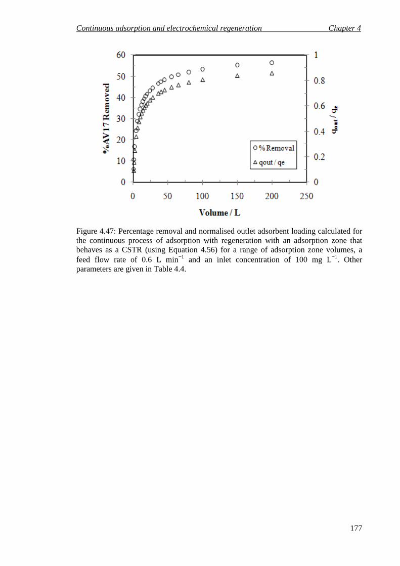
Continuous adsorption and electrochemical regeneration Chapter 4
177
Figure 4.47: Percentage removal and normalised outlet adsorbent loading calculated for the continuous process of adsorption with regeneration with an adsorption zone that behaves as a CSTR (using Equation 4.56) for a range of adsorption zone volumes, a feed flow rate of 0.6 L min−1 and an inlet concentration of 100 mg L−1. Other parameters are given in Table 4.4.
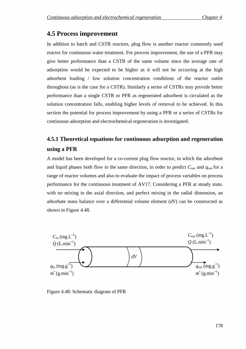
Continuous adsorption and electrochemical regeneration Chapter 4
178
4.5 Process improvement
In addition to batch and CSTR reactors, plug flow is another reactor commonly used
reactor for continuous water treatment. For process improvement, the use of a PFR may
give better performance than a CSTR of the same volume since the average rate of
adsorption would be expected to be higher as it will not be occurring at the high
adsorbent loading / low solution concentration conditions of the reactor outlet
throughout (as is the case for a CSTR). Similarly a series of CSTRs may provide better
performance than a single CSTR or PFR as regenerated adsorbent is circulated as the
solution concentration falls, enabling higher levels of removal to be achieved. In this
section the potential for process improvement by using a PFR or a series of CSTRs for
continuous adsorption and electrochemical regeneration is investigated.
4.5.1 Theoretical equations for continuous adsorption and regeneration
using a PFR
A model has been developed for a co-current plug flow reactor, in which the adsorbent
and liquid phases both flow in the same direction, in order to predict Cout and qout for a
range of reactor volumes and also to evaluate the impact of process variables on process
performance for the continuous treatment of AV17. Considering a PFR at steady state,
with no mixing in the axial direction, and perfect mixing in the radial dimension, an
adsorbate mass balance over a differential volume element (dV) can be constructed as
shown in Figure 4.48.
qin (mg.g−1)
m• (g.min−1)
qout (mg.g−1)
m• (g.min−1)
Cout (mg.L−1) Q (L.min−1)
Cin (mg.L−1) Q (L.min−1)
dV
Figure 4.48: Schematic diagram of PFR

Continuous adsorption and electrochemical regeneration Chapter 4
179
Thus considering a material balance for the adsorbate in the element dV:
qmCQ dd •= (4.78)
V
qm
V
CQ
d
d
d
d •−= = − rate of adsorption (mg L−1 min−1) within dV (4.79)
Assuming m equal to m•/Q and combining Equations (4.79) and (4.48), gives:
2
2 1d
d
−
+−=−
••
vv
v qbC
Cbkk
Q
m
V
qm vL (4.80)
where Cv and qv is the concentration and loading in dV, which has spent a time t in the
reactor.
2
vv
v2v
1
−
+= q
bC
Cbk
Q
k
dV
dq L (4.81)
As there is no axial mixing in the reactor dV can be considered to behave as a batch
reactor, thus:
)(d)(d inin qqWCCV vv −=− (4.82)
where dW is the amount of adsorbent in dV (g). Assuming complete regeneration (so, qin
= 0) and rearranging Equation (4.82) we obtain:
vinv qV
WCC
d
d−= (4.83)
where (dW/dV) is equal to (m•/Q), thus
vv qQ
mCC
•
−= in (4.84)
Substituting Equation (4.84) into Equation (4.81):
2
in
in
2
1
−
−+
−
=•
•
v
v
vL
v q
mCb
mCbk
Q
k
dV
dq (4.85)
Solving Equation (4.85) by a numerical method (Euler integration) using MATLAB
with suitable boundary conditions (at the inlet V = 0, qv = 0 and at the outlet V = V, qv =
qout) (the MATLAB program can be found in Appendix D) and step size h = 0.001,
gives the dye loading under flow condition for adsorption with regeneration in a co-
current PFR. Tests were carried out with a range of values of h to ensure that the step
size was sufficiently small to obtain accurate results (see Appendix E).
Continuous adsorption and electrochemical regeneration Chapter 4
180
An overall adsorbate mass balance for the PFR, gives:
outoutinin qmQCqmQC •• +=+ (4.86)
Thus Cout can be obtained directly from the calculated value of qout:
outinout qQ
mCC
•
−= (4.87)
4.5.2 Comparison of CSTR and co-current PFR performance
In order to compare the performance of continuous adsorption with regeneration in a co-
current PFR with a CSTR, the behaviour was examined under a range of operating
conditions. When performing a sensitivity analysis for any reactor or process, it is
important to select parameter values within a typical operating range in order to
understand the influence of the parameters on the behaviour.
In order to study the possibility of process improvement, a comparison between the co-
current PFR and CSTR adsorption zone systems was carried out for a range of feed flow
rates at an inlet concentration of 100 mg L−1, and for an adsorption zone volume of 36 L
as shown Figure 4.49. The results show that a higher percentage removal was obtained
for the PFR than the CSTR model in all cases, due to the higher rate of removal
achieved in the PFR adsorber than in the CSTR as shown in Figure 4.50. However, the
improvement in performance obtained is relatively small.

Continuous adsorption and electrochemical regeneration Chapter 4
181
Figure 4.49: Comparison of co-current PFR and CSTR systems for percentage removal of AV17 by continuous adsorption with regeneration at a feed concentration of 100 mg L−1 and an adsorption zone volume of 36 L.
Figure 4.50: Comparison of co-current PFR and CSTR adsorption systems for rate removal of AV17 (mg min−1) for continuous adsorption with regeneration at a feed concentration of 100 mg L−1 and a volume of 36 L.

Continuous adsorption and electrochemical regeneration Chapter 4
182
The percentage removal of AV17 achieved using a co-current PFR and CSTR were
compared for a range of adsorption zone volumes at a feed concentration of 100 mg L−1
and a feed flow rate of 1 L min−1 (see Figure 4.51). As expected percentage removal
increased with volume, and the percentage AV17 removal achieved for the same
volume reactor were higher with a co-current PFR than a CSTR. Although the
difference in removal achieved using a co-current PFR and CSTR was relatively small
in Figure 4.49, Figure 4.51 makes it clear that a significantly larger CSTR would be
required to achieve a given level of removal when compared to a co-current PFR.
Figure 4.51: Comparison of PFR and CSTR model to percentage removal of AV17 for adsorption and electrochemical regeneration at a feed concentration of 100 mg L−1 and a feed flow of 0.6 L min−1.
In addition to the single CSTR model (Equation 4.56), the behaviour of n CSTR
systems in series (with circulating regenerated adsorbent in each system) was also
investigated for initial concentration of 100 mg L−1 and feed flow rate of 1 L min−1. This
system was modelled by solving each CSTR (Equation 4.56) individually in turn, so the
outlet concentration Cout from the first reactor became the inlet concentration Cin for the
second reactor and so on. For n CSTR systems in series, the volume of each adsorption
zone was taken as V / n, so that the total adsorption zone volume remained constant. As
n was increased, it was found that the percentage removal increased significantly (see

Continuous adsorption and electrochemical regeneration Chapter 4
183
Figure 4.52), giving significantly higher removal than the single CSTR and co-current
PFR systems.
Figure 4.52: Calculated percentage removal of AV17 achieved with n CSTR continuous adsorption with regeneration systems in series for an inlet concentration 100 mg L−1, a feed flow rate of 1 L min−1, and a fixed total adsorption zone volume of nV = 36 L.
Comparison of Figure 4.49 and Figure 4.52 shows that the percentage removal of AV17
achieved using a co-current PFR was lower than that for 2−6 CSTRs in series. This can
be explained by considering that in the co-current PFR no fresh adsorbent is added and
the adsorbent becomes loaded as it flows along the reactor. With n CSTRs in series
fresh or regenerated adsorbent is circulated in each CSTR, so that higher removal can be
achieved.
This is an important observation as it suggests that for applications where a high
percentage removal is required it is likely that a series of CSTR systems will be more
effective than a PFR design, negating the need to develop a system that achieved a PFR
like RTD in the adsorption zone. However, counter current systems are widely used in
unit operations in chemical engineering such as heat transfer, distillation, absorption and
solvent extraction (Wu and Tseng, 2008). Using a counter current system for adsorption
can reduce the amount of adsorbent required and improve mass transfer (Wu and Tseng,
2008). With a co-current system it is impossible to approach equilibrium with a loaded

Continuous adsorption and electrochemical regeneration Chapter 4
184
adsorbent at the outlet, but with a counter current system fresh (regenerated) adsorbent
at the outlet would be contacted with the contaminated water and thus a high organic
dye removal could be achieved. Thus, much better performance may be possible if such
a system could be designed.
As discussed in Chapter 3, work is being carried out at the University of Manchester to
develop new adsorbent materials suitable for electrochemical regeneration but with
increased adsorptive capacity compared to Nyex®1000 (Asghar, 2011). Hence, the
effect of the adsorptive capacity, kL (mg g−1), was investigated on the behaviour of a
series of CSTRs. A constant adsorbent circulation rate was assumed, m• = 43 g min−1 for
this study. As kL was increased, it was found that the number of CSTRs required to
achieve 99% removal decreased (see Figure 4.53). For example, a doubling of the
adsorbent capacity (as has already been achieved by Asghar (2011) leads to a reduction
in the number of CSTR in series required from 13 to only 4.
Figure 4.53: Effect of adsorptive capacity (kL) on the number of CSTRs required to achieve 99% removal of AV17 (with an initial concentration of 100 mg L−1) for continuous adsorption with regeneration at a flow rate of 1 L min−1, and a fixed total adsorption zone volume of nV = 36 L.

Continuous adsorption and electrochemical regeneration Chapter 4
185
4.6 Conclusions This study has demonstrated that continuous treatment of water by adsorption and
electrochemical regeneration can be effective for the removal and oxidation of dissolved
organic contaminants. The treatment process was able to remove more than 90% of
AV17 in a single pass system from a feed solution containing up to about 100 mg L−1 of
AV17 at a flow rate 0.25 L min−1 (see Table 4.2).
The process requires minimal addition of chemicals (salt and acid for the catholyte) and
does not produce any sludge or liquid waste streams. The results suggest that there is
significant potential for the process in a wide range of water and wastewater treatment
applications. Further work will be needed to demonstrate performance on real effluents
which may contain a mixture of contaminants and this could be considered as an option
for future work. In addition the duration of the experiments described in this research
was a few hours, and the stability of operation over many thousands of hours would
need to be demonstrated for practical application.
The adsorption zone was found to behave as a continuous stirred tank. Using this
observation and measurements of the rate of flow and concentration of the adsorbent,
simple models of the process for adsorption with / without regeneration have been
developed which show good agreement with the experimental results for a given set of
operating conditions. These models are based on adsorption kinetic and isotherm data
which would be relatively easy to obtain for real wastewaters using bench scale
experiments such as those described in this thesis (Chapter 3). Where a mixture of
contaminants are present a combined measure such as COD could be used, although the
models described here would not be able to address selective removal from a mixture of
contaminants.
The process also operates at relatively low powers typically 25 – 35 W during the
experiments described in this chapter, corresponding to 0.56 to 2.33 kWh per m3 for the
range of flow rates studied (0.25 – 0.75 L min−1). When current was applied, hydrogen
was generated at the cathode and the rate of generation of this gas was about 6.3 L h−1
(estimated using Faraday’s law, for further details of the hydrogen production
calculation, see Appendix C). The hydrogen gas can be diluted with the air used to
fluidise the adsorption zone, and in this case the concentration of hydrogen was
estimated to be around 0.00031vol% in the air, which is significantly lower than the
explosive limit, 4.1vol% (Lewis, 2004).

Continuous adsorption and electrochemical regeneration Chapter 4
186
The process models developed were used to investigate the effect of the design and
operating parameters on the process performance for continuous water treatment by
adsorption with regeneration. The adsorption and regeneration model is able to predict
the concentration and adsorbent loading at the outlet (Cout and qout) using the isotherm
and kinetics parameters.
In order to investigate whether a change in the adsorption zone RTD behaviour would
improve the process performance, a co-current PFR model was developed. Sensitivity
analysis was carried out for the co-current PFR and the behaviour of this model was
found to be similar for that of CSTR with respect to the feed flow rates, inlet
concentration, and volume of the system, but with higher dye removal. However, it was
found that significantly higher removals could be achieved with a series of CSTRs with
adsorbent regeneration and circulation in each CSTR. It was also found that the
predicted number of CSTR in series required to achieve 99% AV17 removal was
reduced from 13 to only 4 if the adsorptive capacity of the adsorbent was doubled. Such
a system can readily be designed using the existing process design with a number of
units connected in series. However, development of a counter current PFR system
should also be considered as it is likely that this may be able to achieve higher dye
removal than co-current or CSTR systems.
Conclusions and suggestions for future work Chapter 5
187
CHAPTER 5
CONCLUSIONS AND SUGGESTIONS FOR FUTURE WORK
This research aimed to develop a design model for batch and continuous water
treatment by adsorption and electrochemical regeneration occurring in a single unit (the
Arvia® Process). In addition, the possibility of process improvement to achieve a higher
rate of contaminant removal was considered. This chapter summarises the main
conclusions drawn from this research and gives suggestions for future work.
5.1 Conclusions The process of adsorption with electrochemical regeneration has the potential to be a
significant breakthrough in water treatment technology. This work describes for the first
time the modelling and validation of both the batch and the continuous process using an
organic dye, Acid Violet 17 (AV17), as a model contaminant. The numerical models
were found to be in good agreement with the experimental data and allow process
performance to be calculated provided some simple equilibrium and rate data are
known. All of the main objectives of this study outlined in Chapter one (section 4.1)
have been successfully met. The study has been divided into two broad areas: batch and
continuous processing:
5.1.1 Batch water treatment
The removal and destruction of AV17 from aqueous solution by adsorption and
electrochemical regeneration using a graphite intercalation compound (GIC) adsorbent
was investigated.
• The GIC (Nyex®1000) adsorbent was found to be capable of removing AV17
from aqueous solution with an equilibrium time about 1 h. The Langmuir
isotherm and pseudo second order kinetic model were used to characterise the
experimental data. The maximum adsorption capacity of the GIC was found to
be around 1±0.05 mg of AV17 per g of adsorbent. Although this maximum

Conclusions and suggestions for future work Chapter 5
188
adsorption capacity is significantly lower than typical industrial adsorbents, if it
is normalised by the BET surface area it is about two to three times that of
activated carbon adsorbents.
• The rate constant obtained from the pseudo second-order model, k2, at a range
of initial concentrations was found to be equal to 0.41 g mg−1 min−1 and the
Langmuir adsorptive capacity, kL, was observed to be about 0.987 mg g−1.
• Increasing the temperature of the dye solution was found to increase the rate of
adsorption and the activation energy of the adsorption process was found to be
4.2 kJ mole−1 suggesting that the mechanism of adsorption was physisorption.
Increasing temperature was also found to increase the capacity of the
Nyex®1000. For the range of pH studied, the highest adsorbent capacity was
obtained at pH=2.
• The key advantage of this adsorbent however, is that its initial adsorption
capacity can be fully recovered by anodic electrochemical regeneration in a
packed bed electrochemical cell with a charge passed of 15 C g−1 of adsorbent,
a bed depth of 20 mm and a current density of 7 mA cm−2. The results indicated
that the high electrical conductivity of the adsorbent enables electrochemical
oxidation of adsorbed contaminants with relatively low energy input.
• A multi-stage batch treatment design model (with electrochemical regeneration
after each batch treatment) was developed in order to predict the amount of
adsorbent required per litre of contaminated water. The model was found to be
in good agreement with experimental results for five stages of the adsorption /
regeneration process (see Chapter 3). It was found that the predicted number of
stages of batch adsorption / regeneration required to achieve 99.9% was halved
when the adsorptive capacity of the adsorbent was doubled. This model would
be suitable for design and optimisation of industrial applications of the
adsorption / electrochemical regeneration using the sequential batch approach.
5.1.2 Continuous water treatment The continuous process of adsorption with electrochemical regeneration, developed at
the University of Manchester and being commercialised by Arvia® Technology Ltd,
uses an airlift reactor for continuous water treatment. The design is similar to an annulus

Conclusions and suggestions for future work Chapter 5
189
airlift reactor; but with a rectangular rather than cylindrical construction and with a
moving packed bed electrochemical cell in the downcomer. The process was operated
using the same GIC adsorbent, Nyex®1000, as was used in the batch process. The main
advantages of this process design are: the simple mechanical design; the simple
operation with no moving parts; in situ regeneration of the adsorbent; minimal addition
of chemicals (salt and acid for the catholyte); and no solid or liquid wastes are
produced. In addition, the process operates with relatively low electrical power
consumption typically 25 – 35 W (corresponding to around 0.5 – 2.5 kWh per m3 of
treated water for the range of flow rates studied) during the experiments described in
Chapter 4 and produces a low amount of hydrogen at a rate of 6.3 L h−1 (which gives a
concentration of around 0.0003vol% when it is mixed with the air). In contrast, the
energy consumption for electrochemical regeneration of AC was significantly higher at
around 14.25 kWh per m3 of treated water at 3.25 L min−1 (Zhou et al., 2006) .The main
conclusions for the continuous water treatment process can be summarised as follows:
• Based on residence time distribution studies, the mixing characteristic of the
adsorption zone in the process was found to be similar to that of a CSTR.
• Continuous treatment of water by adsorption with electrochemical regeneration
was found to be effective for the removal and destruction of dissolved organic
contaminants by anodic oxidation. This process was able to remove more than
90% of AV17 from a feed concentration of up to 100 mg L−1 at a flow rate 0.25
L min−1. A numerical model of the continuous adsorption process with complete
regeneration in the electrochemical cell was developed. In addition to
parameters associated with the adsorption kinetics and isotherm, the model
solution depended upon the concentration of adsorbent in the adsorption zone
and the adsorbent circulation rate. Using experimental measurements of all of
these parameters, both the steady state and dynamic variation of the outlet
contaminant concentration predicted by the model was found to be in good
agreement with experimental results. The key data required for the model was
the adsorption kinetics and equilibrium isotherm parameters determined from
bench scale experiments and these parameters would be relatively easy to obtain
for a real wastewater applications. The steady state and dynamic models were
found to be in good agreement with the experiment data for a range of operating
conditions.

Conclusions and suggestions for future work Chapter 5
190
• A numerical model for the continuous water treatment by adsorption with no
regeneration was also developed which shows good agreement with the
experimental results for a given set of operating conditions.
• In terms of process improvement, a PFR was anticipated to give better
adsorption and removal. In order to evaluate this potential, a model was
developed for a co-current PFR adsorption system with regenerated adsorbent
fed to the inlet of the adsorption zone. A sensitivity analysis was undertaken to
study the process performance for a range of design and operating conditions.
The removal and adsorbent capacity for a co-current PFR was found to be higher
than a single CSTR, which indicates the possibility of process improvement.
However, a number of CSTRs in series was found to be a better option since
regenerated adsorbent was circulated as the contaminant was removed from the
treated water. It is likely that a counter current PFR could achieve higher dye
removal than the co-current PFR, and further work should be carried out to
investigate this possibility. It was also found that the predicted number of
CSTRs in series required to achieve 99% AV17 removal was reduced by two
thirds when the adsorptive capacity of the adsorbent was doubled.
• A sensitivity analysis was performed to study the effect of the key design and
operating parameters on the process performance. The feed flow rate was found
to have more effect than the volume of the system and the feed concentration in
terms of contaminant removal by the continuous process of adsorption with
regeneration.
Overall therefore, the Arvia® Process of water treatment by adsorption with
electrochemical regeneration looks to be very promising in both sequential batch and
continuous operation and there is further potential to improve the process by future
developments. Simulations of both the batch and continuous processes have provided a
number of models which agree with the experimental data and should aid future
developments and applications of the process. All of the objectives laid down at the start
of this work have been successfully met.
Conclusions and suggestions for future work Chapter 5
191
5.2 Recommendations for future work
5.2.1 Process improvement
The possibilities for process improvement and the recommended future studies of the
process of adsorption with electrochemical regeneration in the future include:
• CSTRs in series
As discussed in Chapter 4 the mixing behaviour of the treatment process is equivalent to
that of a single CSTR. Thus, in order to improve the process performance with respect
to contaminant removal, for a fixed volume, a series of CSTRs of equal size could
deliver improved performance. CSTRs in series are widely applied in chemical
engineering processes and high removal rates could be achieved. Such a series of
reactors will involve a larger capital expenditure and footprint, but operating
expenditure will be much the same and removal rates should be much improved.
• Plug flow reactor
A co-current plug flow reactor is another possibility for process improvement. This
reactor was discussed in Chapter 4 and the results show the rate of removal for a PFR is
higher than that of single CSTR. Capital expenditure, operating expenditure and
footprint should all be around the same as for a single CSTR. However, the
performance was found to be poorer than a series of CSTR, suggesting that this
approach should not be pursued. However, a counter current PFR design would lead to
a higher rate of adsorption from the liquid phase. This configuration of design is widely
used in heat exchangers, adsorbers, and solvent extraction systems due to the high
performance which can be achieved. The possibility of developing a counter-current
PFR design, where the adsorbent flows in the opposite direction (due to gravity or other
forces such as the use of a magnetic field) to the water being treated, should be
investigated.
5.2.2 Recommendations for process scale-up studies
Process scale-up studies for continuous adsorption with electrochemical regeneration
have been carried out by Arvia® Technology Ltd, based on a stack of electrochemical
regeneration cells mounted in a large single tank which is used as the adsorption zone.
Conclusions and suggestions for future work Chapter 5
192
In this study, experiments have been carried out using the Arvia multi-cell system,
which consisted of a large rectangular tank adsorption zone (volume of 1.3 m3) with a
stack of four electrochemical cells for electrochemical regeneration, (details and results
of this study are included in Appendix B). Experiments were performed to study the
characteristics and performance of the process for adsorption and electrochemical
regeneration. RTD studies indicated that the mixing behaviour of the adsorption zone in
the multi-cell process was again similar to a single CSTR, as observed for the single cell
systems discussed in this thesis (see Appendix B). Experiments were carried out to
investigate the performance of the multi-cell process for adsorption with
electrochemical regeneration at a range of applied currents. The results of these studies
suggested that the electrochemical regeneration in the multi-cell system was not as
effective as expected. It was concluded that this was due to the difficulty of achieving
stable and steady movement of the adsorbent bed inside all of the four cells in the
regeneration zone.
If the multiple cell system is to be pursued, it is recommended that further work is
carried out to investigate the flow and circulation of the adsorbent in the multi-cell
stack. Since it is difficult to observe the bed movement directly it is recommended that a
device for detecting and measuring the bed flow in the multi-cell process based is
developed, possibly using an inductive electrical approach.
5.2.3 Further recommendations for future work
It is recommended that further future work is undertaken as follows:
• Develop a mathematical model for the regeneration zone in order to identify the
limiting step in the regeneration process.
• Develop a transient model for the process, including models of both the
adsorption zone (which has been developed in this thesis), and the regeneration
zone.

References
193
REFERENCES
AHMAD, A. L., PUASA, S. W. & ZULKALI, M. M. D. (2006) Micellar-enhanced ultrafiltration for removal of reactive dyes from an aqueous solution. Desalination, 191, 153-161.
AHMED, M. M. (2008) Electrochemical oxidation of Acid Yellow and Acid Violet dyes assisted by transition metal modified kaolin Portugaliae Electrochimica Acta, 26, 547-557.
AKSU, Z. & KUTSAL, T. (1991) A bioseparation Process for Removing Lead(II) Ions from Waste-Water by Using C-Vulgaris. Journal of Chemical Technology and Biotechnology, 52, 109-118.
ALKAN, M., DOGAN, M., TURHAN, Y., DEMIRBAS, Ö. & TURAN, P. (2008) Adsorption kinetics and mechanism of maxilon blue 5G dye on sepiolite from aqueous solutions. Chemical Engineering Journal, 139, 213-223.
ALLÈGRE, C., MOULIN, P., MAISSEU, M. & CHARBIT, F. (2006) Treatment and reuse of reactive dyeing effluents. Journal of Membrane Science, 269, 15-34.
AN, H., QIAN, Y., GU, X. & TANG, W. Z. (1996) Biological treatment of dye wastewaters using an anaerobic-oxic system. Chemosphere, 33, 2533-2542.
ANNADURAI, G., JUANG, R.-S. & LEE, D.-J. (2002) Use of cellulose-based wastes for adsorption of dyes from aqueous solutions. Journal of Hazardous Materials, 92, 263-274.
ARVIA TECHNOLOGY LTD. (2010) Arvia Technology on-line Liverpool, http://www.arviatechnology.com/process.html.
ASGHAR, H. M. A. (2011) PhD thesis. Development of graphitic adsorbents for water treatment using adsorption and electrochemical regeneration. School of Chemical Engineering and Analytical Science Manchester, UK, University of Manchester.
BAKKER, W. A. M., VANCAN, H. J. L., TRAMPER, J. & DEGOOIJER, C. D. (1993) Hydrodynamics and mixing in a multiple airlift-loop reactor. Biotechnology and Bioengineering, 42, 994-1001.
BANERJEE, K., CHEREMISINOFF, P. N. & CHENG, S. L. (1997) Adsorption kinetics of O-xylene by flyash. Water Research, 31, 249-261.

References
194
BERENGUER, R., MARCO-LOZAR, J. P., QUIJADA, C., CAZORLA-AMOROÌ S, D. & MORALLOÌ N, E. (2010) Comparison among Chemical, Thermal, and Electrochemical Regeneration of Phenol-Saturated Activated Carbon Energy & Fuels, 24, 3366-3372.
BILLO, E. J. (2001) Excel for chemists: A comprehensive guide USA, John Wiley & Sons, Inc.
BOYCE, W. E. & DIPRIMA, R. C. (1997) Elementary differential equations and boundary value problems, USA, New York, John Wiley & Sons, Inc.
BROWN, N. W. (2005) PhD thesis. Adsorption and electrochemical regeneration for wastewater treatment-development of a process. School of Chemical Engineering and Analytical Science. Manchester, UMIST.
BROWN, N. W. & ROBERTS, E. P. L. (2007) Electrochemical pre-treatment of effluents containing chlorinated compounds using an adsorbent. Journal of Applied Electrochemistry, 37, 1329-1335.
BROWN, N. W. & ROBERTS, E. P. L. (2009) Arvia process design. Manchester, Arvia Technology Ltd.
BROWN, N. W., ROBERTS, E. P. L., CHASIOTIS, A., CHERDRON, T. & SANGHRAJKA, N. (2004a) Atrazine removal using adsorption and electrochemical regeneration. Water Research, 38, 3067-3074.
BROWN, N. W., ROBERTS, E. P. L. & ECCLESTON, K. T. (2007) Apparatus for the electrochemical regeneration of absorbents. UK, World Patent No.125334
BROWN, N. W., ROBERTS, E. P. L., GARFORTH, A. A. & DRYFE, R. A. W. (2004b) Electrochemical regeneration of a carbon-based adsorbent loaded with crystal violet dye. Electrochimica Acta, 49, 3269-3281.
BROWN, N. W., ROBERTS, E. P. L., GARFORTH, A. A. & DRYFE, R. A. W. (2004c) Treatment of dyehouse effluents with a carbon-based adsorbent using anodic oxidation regeneration. Water Science and Technology, 49, 219-225.
BULUT, Y. & AYDIN, H. (2006) A kinetics and thermodynamics study of methylene blue adsorption on wheat shells. Desalination, 194, 259-267.
CARLIELL, C. M., BARCLAY, S. J., NAIDOO, N., BUCKLEY, C. A., MULHOLLAND, D. A. & SENIOR, E. (1995) Microbial decolorization of a reactive azo-dye under anaerobic conditions. Water Sa, 21, 61-69.

References
195
CENTRONE, A., BRAMBILLA, L. & ZERBI, G. (2005) Adsorption of H2 on carbon-based materials: A Raman spectroscopy study. Physical Review B, 71, 245406.
CHAKRABORTY, S., PURKAIT, M. K., DASGUPTA, S., DE, S. & BASU, J. K. (2003) Nanofiltration of textile plant effluent for color removal and reduction in COD. Separation and Purification Technology, 31, 141-151.
CHEREMISINOFF, N. P. (2002) Handbook of Water and WastewaterTreatment Technology, United States of America, Butterworth-Heinemunn.
CHERN, J.-M. & CHIEN, Y.-W. (2002) Adsorption of nitrophenol onto activated carbon: isotherms and breakthrough curves. Water Research, 36, 647-655.
CHHABRA, M., MISHRA, S. & SREEKRISHNAN, T. R. (2009) Laccase/mediator assisted degradation of triarylmethane dyes in a continuous membrane reactor. Journal of Biotechnology, 143, 69-78.
CHISTI, M. Y., HALARD, B. & MOOYOUNG, M. (1988) Liquid Circulation in Airlift Reactors. Chemical Engineering Science, 43, 451-457.
CHRISTY, A. A. (2008) Quantitative determination of surface area of silica gel particles by near infrared spectroscopy and chemometrics. Colloids and Surfaces A: Physicochemical and Engineering Aspects, 322, 248-252.
CHU, W. & MA, C.-W. (2000) Quantitative prediction of direct and indirect dye ozonation kinetics. Water Research, 34, 3153-3160.
CIARDELLI, G. & RANIERI, N. (2001) The treatment and reuse of wastewater in the textile industry by means of ozonation and electroflocculation. Water Research, 35, 567-572.
CLARK, R. M. & BENJAMIN, W. L. (1989) Granular activated carbon: Design, Operation and Cost, Michigan, United State of America, Lewis.
CLAUDEL, S., FONTEIX, C., LECLERC, J. P. & LINTZ, H. G. (2003) Application of the possibility theory to the compartment modelling of flow pattern in industrial processes. Chemical Engineering Science, 58, 4005-4016.
COLLIVIGNARELLI, C. & BERTANZA, G. (1996) Oxidising agents for bioresistant pollution treatment. Inquinamento, 8, 68 - 73.
COMNINELLIS, C. & PULGARIN, C. (1991) Annodic-oxidation of phenol for waste-water treatment. Journal of Applied Electrochemistry, 21, 703-708.
COONEY, D. O. (1999) Adsorption design for wastewater treatment, Florida, United States of America, CRC Press LLC.

References
196
COONEY, D. O., NAGERL, A. & HINES, A. L. (1983) Solvent regeneration of activated carbon. Water Research, 17, 403-410.
CULP, R. L., WESNER, G. M. & CULP, G. L. (1978) Handbook of advanced wastewater treatment, Van Nostrand Reinhold, New York.
DAIFULLAH, A. A. M. & GIRGIS, B. S. (1998) Removal of some substituted phenols by activated carbon obtained from agricultural waste. Water Research, 32, 1169-1177.
DAVID, R. W. & GEOFFREY, H. (1990) The Chemistry and application of dyes, New York and London, Plenum Press.
DECHOW, F. J. (1989) Separation and purification techniques in biotechnology, Park Ridge, New Jersey, Noye publication.
DEMIRBAS, E., KOBYA, M. & SULAK, M. T. (2008) Adsorption kinetics of a basic dye from aqueous solutions onto apricot stone activated carbon. Bioresource Technology, 99, 5368-5373.
DEMMING, S., GAUTIER, A., LEGALLAIS, C. & OULD-DRIS, A. (2008) Solid-liquid mass transfers in an Airlift Reactor incorporating alginate beads for the application as a bioartificial liver. Chemical Engineering and Processing: Process Intensification, 47, 2370-2378.
DOGAN, M., ALKAN, M. & ONGANER, Y. (2000) Adsorption of methylene blue from aqueous solution onto perlite. Water Air and Soil Pollution, 120, 229-248.
DORAISWAMY, L. K. (2001) Organic Synthesis Engineering, Oxford University Press.
DORMAND, J. R. & PRINCE, P. J. (1980) A family of embedded Runge-Kutta formulae. Journal of Computational and Applied Mathematics, 6, 19-26.
EDZWALD, J. K. (1993) Coagulation in drinking water treatment-particles, organics and coagulants. Water Science and Technology, 27, 21-35.
EL-KHAIARY, M. I. (2007) Kinetics and mechanism of adsorption of methylene blue from aqueous solution by nitric-acid treated water-hyacinth. Journal of Hazardous Materials, 147, 28-36.
EL QADA, E. N., ALLEN, S. J. & WALKER, G. M. (2008) Adsorption of basic dyes from aqueous solution onto activated carbons. Chemical Engineering Journal, 135, 174-184.
ENOKI, T., SUZUKI, M. & ENDO, M. (2003) Graphite intercalation compounds and applications, Oxford, University press.

References
197
EPA (1989) Technologies for upgrading existing or designing new drinking water treatment facilities. United State, EPA Technology Transfer Report EPA/625/4-89/023
FERRO-GARCIA, M. A., JOSÉ, R.-U., ISIDORA, B.-T. & CARLOS, M.-C. (1996) Chemical and thermal regeneration of an activated carbon saturated with chlorophenols. Journal of Chemical Technology & Biotechnology, 67, 183-189.
FERRO-GARCÍA, M. A., UTRERA-HIDALGO, E., RIVERA-UTRILLA, J., MORENO-CASTILLA, C. & JOLY, J. P. (1993) Regeneration of activated carbons exhausted with chlorophenols. Carbon, 31, 857-863.
FILIPKOWSKA, U. (2004) Efficiency of Black DN adsorption onto chitin in an air-lift reactor. Polish Journal of Environmental Studies, 13, 503-508.
FILIPKOWSKA, U. & WARAKSA, K. (2008) Adsorption of reactive dye on chitosan in air-lift reactor. Adsorption-Journal of the International Adsorption Society, 14, 815-821.
FINDON, A., MCKAY, G. & BLAIR, H. S. (1993) Transport studies for the sorption of copper ions by chitosan. Journal of Environmental Science and Health Part a-Environmental Science and Engineering & Toxic and Hazardous Substance Control, A28, 173-185.
FOGLER, S. H. (1999) Elements of Chemical Reaction Engineering, New Jersey, Prentice Hall.
FOLKMAN, Y. & WACHS, A. M. (1973) Removal of algae from stabilization pond effluents by lime treatment. Water Research, 7, 419-428, IN1, 429-435.
FORGACS, E., CSERHÁTI, T. & OROS, G. (2004) Removal of synthetic dyes from wastewaters: a review. Environment International, 30, 953-971.
GUNAY, A. (2007) Application of nonlinear regression analysis for ammonium exchange by natural (Bigadiç) clinoptilolite. Journal of Hazardous Materials, 148, 708-713.
GUO, Y., YANG, S., FU, W., QI, J., LI, R., WANG, Z. & XU, H. (2003) Adsorption of malachite green on micro- and mesoporous rice husk-based active carbon. Dyes and Pigments, 56, 219-229.
GUO, Y. X., RATHOR, M. N. & TI, H. C. (1997) Hydrodynamics and mass transfer studies in a novel external-loop airlift reactor. Chemical Engineering Journal, 67, 205-214.

References
198
GUPTA, G. S., PRASAD, G. & SINGH, V. N. (1990) Removal of chrome dye from aqueous solutions by mixed adsorbents: Fly ash and coal. Water Research, 24, 45-50.
GUTERMAN, M. M. & NITECKI, Z. H. (1984) Differential Equations: a first course Philadelphia ; London : Saunders College Publishing.
HALL, K. R., EAGLETON, L. C., ACRIVOS, A. & VERMEULEN, T. (1966) Pore- and Solid-Diffusion Kinetics in Fixed-Bed Adsorption under Constant-Pattern Conditions. Industrial & Engineering Chemistry Fundamentals, 5, 212-223.
HAMADI, N. K., CHEN, X. D., FARID, M. M. & LU, M. G. Q. (2001) Adsorption kinetics for the removal of chromium(VI) from aqueous solution by adsorbents derived from used tyres and sawdust. Chemical Engineering Journal, 84, 95-105.
HARRIS, A. T., DAVIDSON, J. F. & THORPE, R. B. (2003) The influence of the riser exit on the particle residence time distribution in a circulating fluidised bed riser. Chemical Engineering Science, 58, 3669-3680.
HEIJNEN, J. J., MULDER, A., WELTEVREDE, R., HOLS, J. & VANLEEUWEN, H. (1991) Large-Scale Anaerobic-Aerobic Treatment of Complex industrial-Waste Water Using Biofilm Reactors Water Science and Technology, 23, 1427-1436.
HO, Y. S. & MCKAY, G. (1998a) The kinetics of sorption of basic dyes from aqueous solution by sphagnum moss peat. Canadian Journal of Chemical Engineering, 76, 822-827.
HO, Y. S. & MCKAY, G. (1998b) A two-stage batch sorption optimized design for dye removal to minimize contact time. Process Safety and Environmental Protection, 76, 313-318.
HO, Y. S. & MCKAY, G. (1999a) Batch Lead(II) Removal From Aqueous Solution by Peat: Equilibrium and Kinetics. Process Safety and Environmental Protection, 77, 165-173.
HO, Y. S. & MCKAY, G. (1999b) A kinetic study of dye sorption by biosorbent waste product pith. Resources Conservation and Recycling, 25, 171-193.
HO, Y. S. & MCKAY, G. (2000) Batch sorber design using equilibrium and contact time data for the removal of lead. Water Air and Soil Pollution, 124, 141-153.
HO, Y. S., PORTER, J. F. & MCKAY, G. (2002) Equilibrium isotherm studies for the sorption of divalent metal ions onto peat: Copper, nickel and lead single component systems. Water Air and Soil Pollution, 141, 1-33.
HO, Y. S., WASE, D. A. J. & FORSTER, C. F. (1996) Kinetic studies of competitive heavy metal adsorption by sphagnum moss peat. Environmental Technology, 17, 71-77.

References
199
HUNGER, K. (2003) Industrial dyes: Chemistry, properties, applications, Germany, Wiley-VCH.
HUSSAIN, S. N. (2011) PhD thesis. Electrochemical regeneration of graphite based adsorbents and disinfection of water by adsorption with electrochemical regeneration. School of Chemical Engineering and Analytical Science. Manchester, UK, University of Manchester.
ISIK, M. & SPONZA, D. T. (2006) Biological treatment of acid dyeing wastewater using a sequential anaerobic/aerobic reactor system. Enzyme and Microbial Technology, 38, 887-892.
JOSHI, M. & PURWAR, R. (2004) Developments in new processes for colour removal from effluent. Review of Progress in Coloration and Related Topics, 34, 58-71.
KANNAN, N. & SUNDARAM, M. M. (2001) Kinetics and mechanism of removal of methylene blue by adsorption on various carbons--a comparative study. Dyes and Pigments, 51, 25-40.
KAPOOR, A. & YANG, R. T. (1989) Correlation of equilibrium adsorption data of condensible vapours on porous adsorbents. Gas Separation & Purification, 3, 187-192.
KAYODE COKER, A. (2001) Modeling of chemical kinetics and reactor design, Woburn, Butterworth-Heinemann publications, Wildwood Avenue.
KNOPP, P. V., GITCHEL, W. B., MEIDL, J. A. & BERNDT, C. L. (1978) Wet Oxidation Regeneration. Cheremisinoff, Paul N. and Fred Ellerbusch (Ed.). Carbon Adsorption Handbook. Ix+1054p. Illus. Maps. Ann Arbor Science Publishers Inc.: Ann Arbor, Mich., USA. Isbn 0-250-40236-X, 539-625.
KONSOWA, A. H. (2003) Decolorization of wastewater containing direct dye by ozonation in a batch bubble column reactor. Desalination, 158, 233-240.
KUAI, L., DE VREESE, I., VANDEVIVERE, P. & VERSTRAETE, W. (1998) GAC-amended UASB reactor for the stable treatment of toxic textile wastewater. Environmental Technology, 19, 1111-1117.
KUMAR, K. V. & SIVANESAN, S. (2005) Prediction of optimum sorption isotherm: Comparison of linear and non-linear method. Journal of Hazardous Materials, 126, 198-201.
LAGERGREN, S. (1898) About the theory of so-called adsorption of soluble substances, Kungliga Svenska Vetenskapsakademiens. Handlingar, 24, 1-39.
LANGMUIR, I. (1916) The constitution and fundamental properties of solids and liquids. Part 1. Solids. Journal of the American Chemical Society, 38, 2221-2295.

References
200
LANGMUIR, I. (1918) The Adsorption of Gases on Plane Surfaces of Glass, Mica and Platinum Journal of the American Chemical Society, 40, 1361-1403.
LEE, J.-W., CHOI, S.-P., THIRUVENKATACHARI, R., SHIM, W.-G. & MOON, H. (2006) Evaluation of the performance of adsorption and coagulation processes for the maximum removal of reactive dyes. Dyes and Pigments, 69, 196-203.
LEFRANCOIS, M. H., MARILLER, C. C. & MIJANE, J. V. (1955) Effectiomements aux proceds de cultures forgiques et de Fermentations Industrielles. Brevet d’Invention. No. 1 ed.
LETTERMAN, R. D. (1999) Water Quality and Treatment - A Handbook of Community Water Supplies (5th Edition), McGraw-Hill.
LEVENSPIEL, O. (1999) Chemical Reaction Engineering, New York, John Wiley and Sons.
LEVENSPIEL, O. & SMITH, W. K. (1957) Notes on the Diffusion-Type Model for the Longitudinal Mixing of Fluids in Flow Chemical Engineering Science, 6, 227-233.
LEWIS, R. J., SR. (2004) Sax's Dangerous Properties of Industrial Materials 11th ed., John Wiley & Sons.
MAHMOUD, A. S., GHALY, A. E. & BROOKS, M. S. (2007) Removal of dye from textile wastewater using plant oils under different pH and temperature conditions. American Journal of Environmental Sciences, 3, 205-218.
MAJI, S. K., PALA, A., PAL, T. & ADAK, A. (2007) Modeling and fixed bed column adsorption of As(III) on laterite soil. Separation and Purification Technology, 56, 284-290.
MARMAGNE, O. & COSTE, C. (1996) Color removal from textile plant effluents. American Dyestuff Reports, 85, 15-21.
MARQUARDT, D. W. (1963) An Algorithm for least-squares estimation of nonlinear parameters. Journal of the Society for Industrial and Applied Mathematics, 11, 431-441.
MARTIN, A. D. (2000) Interpretation of residence time distribution data. Chemical Engineering Science, 55, 5907-5917.
MARTIN, R. J. & NG, W. J. (1984) Chemical regeneration of exhausted activated carbon--I. Water Research, 18, 59-73.
MARTÍNEZ-HUITLE, C. A. & BRILLAS, E. (2009) Decontamination of wastewaters containing synthetic organic dyes by electrochemical methods: A general review. Applied Catalysis B: Environmental, 87, 105-145.
References
201
MCKAY, G. (1981) Design models for adsorption systems in wastewater-treatment. Journal of Chemical Technology and Biotechnology, 31, 717-731.
MCKAY, G. (1982) Adsorption of dyestuffs from aqueous solutions with activated carbon I: Equilibrium and batch contact-time studies. Journal of Chemical Technology and Biotechnology, 32, 759-772.
MCKAY, G. (1988) Fluidized bed adsorption of pollutants on to activated carbon. The Chemical Engineering Journal, 39, 87-96.
MCKAY, G., ALLEN, S. J. & MCCONVEY, I. F. (1984) The adsorption of dyes from solution-equilibrium and column studies. Water Air and Soil Pollution, 21, 127-139.
MCKAY, G., EL GEUNDI, M. & NASSAR, M. M. (1987) Equilibrium studies during the removal of dyestuffs from aqueous solutions using Bagasse pith. Water Research, 21, 1513-1520.
MCKAY, G., OTTERBURN, M. S. & AGA, J. A. (1985) Fullers Earth and Fired Clay as Adsorbents for Dyestuffs - Equilibrium and Rate Studies. Water Air and Soil Pollution, 24, 307-322.
MCLAREN, K. (1983) The colour science of dyes and pigments, Bristol, Adam Hilger Ltd.
MERCHUK, J. C. & SIEGEL, M. H. (1988) Air-lift reactors in chemical and biological technology. Journal of Chemical Technology and Biotechnology, 41, 105-120.
MESHKO, V., MARKOVSKA, L., MINCHEVA, M. & RODRIGUES, A. E. (2001) Adsorption of basic dyes on granular acivated carbon and natural zeolite. Water Research, 35, 3357-3366.
MEYER, V., CARLSSON, F. H. H. & OELLERMANN, R. A. (1992) Decolourization of textile effluent using a low-cost natural adsorbent material Water Science and Technology, 26, 1205-1211.
MISHRA, V. S., MAHAJANI, V. V. & JOSHI, J. B. (1995) Wet Air Oxidation. Industrial & Engineering Chemistry Research, 34, 2-48.
MISRA, K., KAPOOR, S. K. & BANSAL, R. C. (2002) Regeneration of granular activated carbon loaded with explosives. Journal of Environmental Monitoring, 4, 462-464.
MOHAMMED, F. M., ROBERTS, E. P. L., HILL, A., CAMPEN, A. K. & BROWN, N. W. (2011) Continuous water treatment by adsorption and electrochemical regeneration. Water Research, 45, 3065-3074.

References
202
MOHAN, D., SINGH, K. P., SINGH, G. & KUMAR, K. (2002) Removal of dyes from wastewater using flyash, a low-cost adsorbent. Industrial & Engineering Chemistry Research, 41, 3688-3695.
MOHANTY, K., DAS, D. & BISWAS, M. N. (2008) Treatment of phenolic wastewater in a novel multi-stage external loop airlift reactor using activated carbon. Separation and Purification Technology, 58, 311-319.
MOLINA, E., CONTRERAS, A. & CHISTI, Y. (1999) Gas Holdup, Liquid Circulation and Mixing Behaviour of Viscous Newtonian Media in a Split-Cylinder Airlift Bioreactor. Food and Bioproducts Processing, 77, 27-32.
MURPHY, O. J., DUNCAN HITCHENS, G., KABA, L. & VEROSTKO, C. E. (1992) Direct electrochemical oxidation of organics for wastewater treatment. Water Research, 26, 443-451.
NAJM, I. N. (1996) Mathematical modeling of PAC adsorption processes. American Water Works Association Journal, 88, 79-89.
NAMASIVAYAM, C., DINESH KUMAR, M., SELVI, K., ASHRUFFUNISSA BEGUM, R., VANATHI, T. & YAMUNA, R. T. (2001) Waste' coir pith--a potential biomass for the treatment of dyeing wastewaters. Biomass and Bioenergy, 21, 477-483.
NAMASIVAYAM, C. & KAVITHA, D. (2002) Removal of Congo Red from water by adsorption onto activated carbon prepared from coir pith, an agricultural solid waste. Dyes and Pigments, 54, 47-58.
NAMASIVAYAM, C., SANGEETHA, D. & GUNASEKARAN, R. (2007) Removal of Anions, Heavy Metals, Organics and Dyes from Water by Adsorption onto a New Activated Carbon from Jatropha Husk, an Agro-Industrial Solid Waste. Process Safety and Environmental Protection, 85, 181-184.
NARBAITZ, R. M. & CEN, J. Q. (1994) Electrochemical Regeneration of Granular Activated Carbon Water Research, 28, 1771-1778.
NARBAITZ, R. M. & KARIMI-JASHNI, A. (2009) Electrochemical regeneration of granular activated carbons loaded with phenol and natural organic matter. Environmental Technology, 30, 27-36.
NAUMCZYK, J., SZPYRKOWICZ, L. & ZILIO-GRANDI, F. (1996) Electrochemical treatment of textile wastewater. Water Science and Technology, 34, 17-24.
NEMR, A. E., ABDELWAHAB, O., EL-SIKAILY, A. & KHALED, A. (2009) Removal of direct blue-86 from aqueous solution by new activated carbon developed from orange peel. Journal of Hazardous Materials, 161, 102-110.

References
203
O'NEILL, C., HAWKES, F. R., HAWKES, D. L., ESTEVES, S. & WILCOX, S. J. (2000) Anaerobic-aerobic biotreatment of simulated textile effluent containing varied ratios of starch and azo dye. Water Research, 34, 2355-2361.
OWEN, P. & BARRY, J. (1972) Electrochemical carbon regeneration. Report Huntington Beach, California. Report number PB 239156 Environics Inc. ÖZACAR, M. (2006) Contact time optimization of two-stage batch adsorber design using second-order kinetic model for the adsorption of phosphate onto alunite. Journal of Hazardous Materials, 137, 218-225.
ÖZACAR, M. & SENGIL, I. A. (2003) Adsorption of reactive dyes on calcined alunite from aqueous solutions. Journal of Hazardous Materials, 98, 211-224.
ÖZACAR, M. & SENGIL, I. A. (2004) Equilibrium data and process design for adsorption of disperse dyes onto alunite. Environmental Geology, 45, 762-768.
ÖZACAR, M. & SENGYL, I. A. (2004) Two-stage batch sorber design using second-order kinetic model for the sorption of metal complex dyes onto pine sawdust. Biochemical Engineering Journal, 21, 39-45.
PANIZZA, M., BOCCA, C. & CERISOLA, G. (2000) Electrochemical treatment of wastewater containing polyaromatic organic pollutants. Water Research, 34, 2601-2605.
PANIZZA, M. & CERISOLA, G. (2001) Removal of organic pollutants from industrial wastewater by electrogenerated Fenton's reagent. Water Research, 35, 3987-3992.
PARIMAL, S., PRASAD, M. & BHASKAR, U. (2010) Prediction of equillibrium sorption isotherm: Comparison of linear and nonlinear methods. Industrial & Engineering Chemistry Research, 49, 2882-2888.
PEEL, R. G. & BENEDEK, A. (1980) Attainment of equilibrium in activated carbon isotherm studies. Environmental Science & Technology, 14, 66-71.
PLETCHER, D. & WALSH, F. C. (1993) Industrial Electrochemistry, London, UK, Balackie Academic and Professional Chapman and Hall.
POHORECKI, R. (2002) Hydrodynamic problems in bioreactors engineering. Chemical Engineering Equipment, 3, 118-120.
PORTER, J. F., MCKAY, G. & CHOY, K. H. (1999) The prediction of sorption from a binary mixture of acidic dyes using single- and mixed-isotherm variants of the ideal adsorbed solute theory. Chemical Engineering Science, 54, 5863-5885.

References
204
RAJESHWAR, K. & IBANER, J. (1996) Environmental Electrochemistry. Fundumentals and Applicantions in pollution Abatement, New York, USA, Academic Press.
RANGNEKAR, D. W. & SINGH, P. P. (1980) An introduction to synthetic dyes, Bombay, Himalaya.
RATKOWSKY, D. A. (1990) Handbook of nonlinear regression models, New York Marcel Dekker Inc.
RENGARAJ, S. & MOON, S. H. (2002) Kinetics of adsorption of Co(II) removal from water and wastewater by ion exchange resins. Water Research, 36, 1783-1793.
REYNOLDS, T. D. & RICHARDS, P. A. (1996) Unit Operations and Process in Environmental Engineering, Boston, United State of America, PWS.
ROBINSON, T., MCMULLAN, G., MARCHANT, R. & NIGAM, P. (2001) Remediation of dyes in textile effluent: a critical review on current treatment technologies with a proposed alternative. Bioresource Technology, 77, 247-255.
SABIO, E., GONZALEZ, E., GONZALEZ, J. F., GONZALEZ-GARCIA, C. M., RAMIRO, A. & GANAN, J. (2004) Thermal regeneration of activated carbon saturated with p-nitrophenol. Carbon, 42, 2285-2293.
SAN MIGUEL, G., LAMBERT, S. D. & GRAHAM, N. J. D. (2001) The regeneration of field-spent granular-activated carbons. Water Research, 35, 2740-2748.
SANGHI, R. & BHATTACHARYA, B. (2002) Review on decolorisation of aqueous dye solutions by low cost adsorbents. Coloration Technology, 118, 256-269.
SARAVANATHAMIZHAN, R., BALASUBRAMANIAN, N. & SRINIVASAKANNAN, C. (2010) Comparison of tank-in-series and axial dispersion models for an electrochemcial reactor. Journal of Modelling and Simulation of Systems, 1, 171-175.
SARAVANATHAMIZHAN, R., PARANTHAMAN, R., BALASUBRAMA NIAN, N. & BASHA, C. A. (2008) Residence time distribution in continuous stirred tank electrochemical reactor. Chemical Engineering Journal, 142, 209-216.
SCHROEDER, E. D. (1977) Water and Wastewater Treatment, Tokyo, McGraw Hill.
SCHWEIGER, T. A. J. & LEVAN, M. D. (1993) Steam regeneration of solvent adsorbers. Industrial & Engineering Chemistry Research, 32, 2418-2429.
SHAH, Y. T. (1979) Gas-liquid-solid Reactor Design New York; London, McGraw-Hill Inc.

References
205
SHAMPINE, L. F., GLADWELL, I. & THOMPSON, S. (2003) Solving ODEs with MATLAB, Cambridge university press, UK.
SHAW, C. B., CARLIELL, C. M. & WHEATLEY, A. D. (2002) Anaerobic/aerobic treatment of coloured textile effluents using sequencing batch reactors. Water Research, 36, 1993-2001.
SHAWABKEH, R. A. & TUTUNJI, M. F. (2003) Experimental study and modeling of basic dye sorption by diatomaceous clay. Applied Clay Science, 24, 111-120.
SHEINTUCH, M. & MATATOV-MEYTAL, Y. I. (1999) Comparison of catalytic processes with other regeneration methods of activated carbon. Catalysis Today, 53, 73-80.
SIGMA ALDRICH (2010) Sigma Aldrich on-line catalogue. http://www.sigmaaldrich.com/catlog/ProductDetial/ALDRICH/210579.
SIVARAJ, R., NAMASIVAYAM, C. & KADIRVELU, K. (2001) Orange peel as an adsorbent in the removal of Acid violet 17 (acid dye) from aqueous solutions. Waste Management, 21, 105-110.
SOOS, M., RAJNIAK, P. & ZAJDLIK, R. (2000) Mathematical and experimental modelling of sorption processes in a fixed bed adsorber. Chemical Papers-Chemicke Zvesti, 54, 489-495.
STREAT, M., PATRICK, J. W. & PEREZ, M. J. C. (1995) Sorption of Phenol and Para-Chlorophenol from Water Using Conventional and Novel Activated Carbons. Water Research, 29, 467-472.
SUN, S. L., LIU, C. J., WEI, W. S. & BAO, X. J. (2006) Hydrodynamics of an annulus airlift reactor. Powder Technology, 162, 201-207.
SUZUKI, M., MISIC, D. M., KOYAMA, O. & KAWAZOE, K. (1978) Study of thermal regeneration of spent activated carbons: Thermogravimetric measurement of various single component organics loaded on activated carbons. Chemical Engineering Science, 33, 271-279.
TAN, B. H., TENG, T. T. & OMAR, A. K. M. (2000) Removal of dyes and industrial dye wastes by magnesium chloride. Water Research, 34, 597-601.
THINAKARAN, N., BASKARALINGAM, P., PULIKESI, M., PANNEERSELVAM, P. & SIVANESAN, S. (2008) Removal of Acid Violet 17 from aqueous solutions by adsorption onto activated carbon prepared from sunflower seed hull. Journal of Hazardous Materials, 151, 316-322.

References
206
THOMAS, H. A., JR. & MCKEE, J. E. (1944) Longitudinal Mixing in Aeration Tanks. Sewage Works Journal, 16, 42-55.
TUNALI, S., ÖZCAN, A. S., ÖZCAN, A. & GEDIKBEY, T. (2006) Kinetics and equilibrium studies for the adsorption of Acid Red 57 from aqueous solutions onto calcined-alunite. Journal of Hazardous Materials, 135, 141-148.
UNUABONAH, E. I., ADEBOWALE, K. O. & OFOMAJA, A. E. (2009) Two-stage Batch Adsorber Design: A Time-Dependent Langmuir Model for Adsorption of Pb2+ and Cd2+ onto Modified Kaolinite Clay. Water Air and Soil Pollution, 200, 133-145.
VADIVELAN, V. & KUMAR, K. V. (2005) Equilibrium, kinetics, mechanism, and process design for the sorption of methylene blue onto rice husk. Journal of Colloid and Interface Science, 286, 90-100.
VAN BENSCHOTEN, J. E. & EDZWALD, J. K. (1990) Chemical aspects of coagulation using aluminum salts--I. Hydrolytic reactions of alum and polyaluminum chloride. Water Research, 24, 1519-1526.
VANDEVIVERE, P. C., BIANCHI, R. & VERSTRAETE, W. (1998) Treatment and reuse of wastewater from the textile wet-processing industry: Review of emerging technologies. Journal of Chemical Technology and Biotechnology, 72, 289-302.
VASANTH KUMAR, K. & SIVANESAN, S. (2006) Equilibrium data, isotherm parameters and process design for partial and complete isotherm of methylene blue onto activated carbon. Journal of Hazardous Materials, 134, 237-244.
VEERARAGHAVAN, S., FAN, L. T. & MATHEWS, A. P. (1989) Modeling adsorption in liquid--solid fluidized beds. Chemical Engineering Science, 44, 2333-2345.
VENKATARAMAN, K. (1952) The chemistry of synthetic dyes, New York, Academic Press Inc.
VERLAAN, P., VAN EIJS, A. M. M., TRAMPER, J., RIET, K. V. T. & LUYBEN, K. C. A. M. (1989) Estimation of axial dispersion in individual sections of an airlift-loop reactor. Chemical Engineering Science, 44, 1139-1146.
VIRARAGHAVAN, T. & WIMMER, C. H. (1988) Polyaluminium chloride as an alternative to alum coagulation: a case study. In. proceedings of Canadian Society of Civil Engineers Annual Conference. Canada.
VLYSSIDES, A. G., PAPAIOANNOU, D., LOIZIDOY, M., KARLIS, P. K. & ZORPAS, A. A. (2000) Testing an electrochemical method for treatment of textile dye wastewater. Waste Management, 20, 569-574.

References
207
WAER, M. A., SNOEYINK, V. L. & MALLON, K. L. (1992) Carbon Regeneration - Dependence on Time and Temperature. Journal American Water Works Association, 84, 82-91.
WALKER, G. M. & WEATHERLEY, L. R. (1998) Fixed bed adsorption of acid dyes onto activated carbon. Environmental Pollution, 99, 133-136.
WALKER, G. M. & WEATHERLEY, L. R. (2000) Prediction of bisolute dye adsorption isotherms on activated carbon. Process Safety and Environmental Protection, 78, 219-223.
WALKER, G. M. & WEATHERLEY, L. R. (2001) Adsorption of dyes from aqueous solution -- the effect of adsorbent pore size distribution and dye aggregation. Chemical Engineering Journal, 83, 201-206.
WANG, S. B., BOYJOO, Y., CHOUEIB, A. & ZHU, Z. H. (2005) Removal of dyes from aqueous solution using fly ash and red mud. Water Research, 39, 129-138.
WANKO, A., ZHANG, J. B., MOSE, R., GREGOIRE, C. & SADOWSKI, A. (2010) Hydraulic parameters and statistical residence time distribution moments correlations - a lysimeter study for pesticides mitigation. International Journal of Environmental Analytical Chemistry, 90, 299 - 310.
WATTERS, J. C., BIAGTAN, E. & SENLER, O. (1991) Ultrafiltration of a textile plant effluent Separation Science and Technology, 26, 1295-1313.
WEBER, W. J. & MORRIS, J. C. (1963) Kinetics of Adsorption on Carbon from Solution. J. sanitation Eng. Div. ASCE, 89, 31-60.
WEN, C. Y. & FAN, L. T. (1975) Models for Flow Systems and Chemical Reactors New York, Marcel Dekker.
WISSLER, M. (2006) Graphite and carbon powders for electrochemical applications. Journal of Power Sources, 156, 142-150.
WU, F. C. & TSENG, R. L. (2008) Liquid-solid phase countercurrent multi-stage adsorption process for using the Langmuir equation. Journal of Hazardous Materials, 155, 449-458.
XU, X.-R., LI, H.-B., WANG, W.-H. & GU, J.-D. (2005) Decolorization of dyes and textile wastewater by potassium permanganate. Chemosphere, 59, 893-898.
YAGI, S. & MIYAUCHI, T. (1953) On the residence time curves of the continuous reactors. Chemical Engineering (Tokyo), 17, 382-386.

References
208
ZAKARIA, N. D., YUSOF, N. A., HARON, J. & ABDULLAH, A. H. (2009) Synthesis and Evaluation of a Molecularly Imprinted Polymer for 2,4-Dinitrophenol. International Journal of Molecular Sciences, 10, 354-365.
ZAOYAN, Y., KE, S., GUANGLIANG, S., FAN, Y., JINSHAN, D. & HUANIAN, M. (1992) Anaerobic aerobic treatment of a dye waste-water by comination of RBC with activated-sludge. Water Science and Technology, 26, 2093-2096.
ZHANG, F., YEDILER, A., LIANG, X. & KETTRUP, A. (2004) Effects of dye additives on the ozonation process and oxidation by-products: a comparative study using hydrolyzed C.I. Reactive Red 120. Dyes and Pigments, 60, 1-7.
ZHANG, H. (2002) Regeneration of exhausted activated carbon by electrochemical method. Chemical Engineering Journal, 85, 81-85.
ZHOU, M. H. & LEI, L. C. (2006) Electrochemical regeneration of activated carbon loaded with p-nitrophenol in a fluidized electrochemical reactor. Electrochimica Acta, 51, 4489-4496.

Appendices
209
APPENDICES

Appendices
210
APPENDIX A
EXPERIMENTAL DATA FOR BATCH PROCESS Table A.1: Effect of AV17 concentration on uptake by Nyex®1000, dosage 20 g L−1.
Time (min)
AV17 concentration (mg L-1)
AV17 loading (mg g−−−−1)
0 26.14 22.84 18.4 13.3 0 0 0 0 2 16 12.77 8.49 4.36 0.51 0.5 0.5 0.45 4 15.45 11.93 7.27 4.34 0.53 0.55 0.56 0.45 6 14.31 11.12 6.82 4.2 0.59 0.59 0.58 0.45 8 13.72 10.54 6.61 3.99 0.62 0.61 0.59 0.46 10 13.58 10.37 6.7 3.77 0.63 0.62 0.59 0.47 12 13.52 10.33 6.13 3.1 0.63 0.63 0.61 0.51 14 13.57 9.9 5.89 3.37 0.63 0.65 0.63 0.5 16 12.43 9.167 5.32 2.99 0.69 0.68 0.65 0.51 18 11.91 9.137 5.28 2.48 0.71 0.69 0.66 0.54 20 11.57 9.034 5.35 1.92 0.73 0.69 0.65 0.57 25 11.44 9.052 4.83 1.48 0.73 0.69 0.68 0.59 30 11.31 8.319 4.64 1.55 0.74 0.73 0.69 0.59 35 10.92 7.958 3.82 1.32 0.76 0.74 0.73 0.6 40 10.83 7.736 3.76 1.31 0.77 0.76 0.73 0.6 45 10.84 7.742 3.67 1.3 0.76 0.75 0.74 0.6 50 10.52 7.622 3.55 1.32 0.78 0.76 0.74 0.6 55 9.858 7.369 3.13 1.18 0.81 0.77 0.76 0.6 60 9.323 7.658 3.25 0.93 0.84 0.76 0.76 0.62 70 9.299 7.333 3.1 0.78 0.84 0.78 0.77 0.62 80 9.016 7.273 2.89 0.67 0.86 0.78 0.78 0.63 90 8.716 7.033 2.64 0.6 0.87 0.79 0.79 0.63 100 8.716 6.624 2.22 0.48 0.87 0.81 0.81 0.64 110 8.68 6.606 2.19 0.48 0.87 0.81 0.81 0.64 120 8.548 6.582 2.18 0.48 0.88 0.81 0.81 0.64 140 8.463 6.522 2.16 0.48 0.88 0.82 0.81 0.64 160 8.566 6.54 2.04 0.54 0.88 0.82 0.82 0.64
180 8.596 6.468 1.77 0.52 0.88 0.82 0.83 0.64

Appendices
211
Table A.2: Effect of AV17 temperature on uptake by Nyex®1000, dosage 20 g L−1.
Time AV17 concentration (mg L−−−−1) AV17 loading (mg g−−−−1)
(min) 30 °C 40 °C 57 °C 66 °C 30 °C 40 °C 57 °C 66 °C 0 21.86 21.86 21.86 21.86 0 0 0 0 2 12.69 11.54 11.33 10.87 0.459 0.516 0.527 0.549 4 12.08 11.11 10.9 10.54 0.489 0.537 0.548 0.566 6 11.37 10.25 10 9.795 0.524 0.58 0.593 0.603 8 10.27 9.831 9.506 8.952 0.58 0.601 0.618 0.645 10 9.88 9.699 9.422 8.928 0.599 0.608 0.622 0.646 12 9.41 8.916 8.807 8.558 0.622 0.647 0.652 0.665 14 8.88 8.59 8.434 7.928 0.649 0.663 0.671 0.696 16 8.735 8.193 8.133 7.639 0.656 0.683 0.686 0.711 18 8.06 7.639 7.47 7.289 0.69 0.711 0.719 0.728 20 7.952 7.47 7.265 7.048 0.695 0.719 0.73 0.74 25 8.012 7.229 7.072 6.651 0.692 0.731 0.739 0.76 30 7.843 7.036 6.699 6.193 0.701 0.741 0.758 0.783 35 7.53 6.651 6.434 5.976 0.716 0.76 0.771 0.794 40 7.47 6.542 6.241 5.88 0.719 0.766 0.781 0.799 45 7.133 6.482 6.048 5.434 0.736 0.769 0.79 0.821 50 6.922 6.265 5.88 5.084 0.747 0.78 0.799 0.839 55 6.717 6 5.771 4.928 0.757 0.793 0.804 0.846 60 6.56 5.723 5.687 4.843 0.765 0.807 0.809 0.851 70 6.06 5.265 5.096 4.723 0.79 0.83 0.838 0.857 80 5.367 5 4.892 4.482 0.824 0.843 0.848 0.869 90 5.205 4.711 4.59 4.337 0.833 0.857 0.863 0.876 100 4.94 4.578 4.506 4.325 0.846 0.864 0.868 0.877 110 4.831 4.398 4.253 4.12 0.851 0.873 0.88 0.887 120 4.759 3.94 3.651 3.373 0.855 0.896 0.91 0.924 140 4.506 3.735 3.446 3.169 0.868 0.906 0.921 0.934 160 3.976 3.205 3.06 2.807 0.894 0.933 0.94 0.952
180 3.373 3.253 2.434 2.265 0.924 0.93 0.971 0.98
Table A.3: Relationship between isotherm equilibrium AV17 concentrations (Ce) and uptake by Nyex®1000 (qe) dosage 20 g L−1.
Co Ce qe
(mg L-1) (mg L-1) (mg g-1)
4.81 1.05 0.188
9.56 1.90 0.38
14.44 4.16 0.51
19.02 6.08 0.65
23.44 8.05 0.77
28.23 11.66 0.83
37.24 20.55 0.83
41.93 25.34 0.83
46.21 28.57 0.88

Appendices
212
Table A.4: Effect of pH of adsorption of AV17 onto Nyex®1000 at initial concentration of 22 mg L−1 and dosage 20 g L−1.
pH Ce (mg L-1) % Removal qe (mg g−1) 2 1.82 91.72 1.01 3 6.49 70.51 0.78 4 10.58 51.92 0.57 5 11.5 47.71 0.52 6 12.2 44.55 0.49 7 12.92 41.25 0.45 8 12.08 45.07 0.5 9 13.19 40.05 0.44
10 12.17 44.68 0.49
11 11.77 46.47 0.51
Figure A.1: UV-Visible spectra of Acid Violet 17 at different pH.
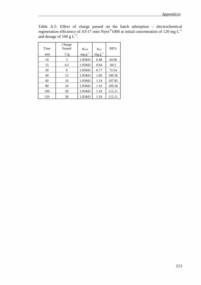
Appendices
213
Table A.5: Effect of charge passed on the batch adsorption – electrochemical regeneration efficiency of AV17 onto Nyex®1000 at initial concentration of 120 mg L−1 and dosage of 100 g L−1.
Time Charge Passed qfresh qreg RE%
min C/g mg g−1 mg g−1
10 3 1.05843 0.48 44.96
15 4.5 1.05843 0.64 60.5
30 9 1.05843 0.77 72.54
40 12 1.05843 1.06 100.56
60 18 1.05843 1.14 107.85
80 24 1.05843 1.16 109.36
100 30 1.05843 1.18 112.11
120 36 1.05843 1.18 112.11

Appendices
214
APPENDIX B
EXPERIMENTAL DATA FOR CONTINUOUS PROCESS Table B.1: RTD test in the single cell small unit by injection of a pulse of NaCl solution (26w %) at 320 mL min−1water flow rate.
Time k C Time k C Time k C Time k C
min ms/cm mg/L min ms/cm mg/L min ms/cm mg/L min ms/cm mg/L
0 0.1031 0.00 65 4.93 3016.81 130 0.591 304.94 195 0.1844 50.81
2.5 2.01 1191.81 67.5 4.52 2760.56 132.5 0.553 281.19 197.5 0.1828 49.81
5 36.3 22623.06 70 4.15 2529.31 135 0.506 251.81 200 0.1795 47.75
7.5 48.1 29998.06 72.5 3.7 2248.06 137.5 0.479 234.94 202.5 0.1788 47.31
10 44.5 27748.06 75 3.44 2085.56 140 0.443 212.44 205 0.175 44.94
12.5 39.5 24623.06 77.5 3.16 1910.56 142.5 0.42 198.06 207.5 0.1717 42.88
15 34.7 21623.06 80 2.87 1729.31 145 0.398 184.31 210 0.1661 39.38
17.5 30.2 18810.56 82.5 2.64 1585.56 147.5 0.37 166.81 212.5 0.1627 37.25
20 26.5 16498.06 85 2.42 1448.06 150 0.356 158.06 215 0.1621 36.88
22.5 23 14310.56 87.5 2.22 1323.06 152.5 0.338 146.81 217.5 0.1611 36.25
25 20 12435.56 90 2.04 1210.56 155 0.321 136.19 220 0.161 36.19
27.5 17.91 11129.31 92.5 1.874 1106.81 157.5 0.3 123.06 222.5 0.161 36.19
30 16.47 10229.31 95 1.701 998.69 160 0.287 114.94 225 0.1598 35.44
32.5 15.15 9404.31 97.5 1.573 918.69 162.5 0.279 109.94 227.5 0.1567 33.50
35 14.13 8766.81 100 1.458 846.81 165 0.272 105.56 230 0.1519 30.50
37.5 13.17 8166.81 102.5 1.342 774.31 167.5 0.264 100.56 232.5 0.151 29.94
40 12.13 7516.81 105 1.242 711.81 170 0.252 93.06 235 0.1496 29.06
42.5 11.19 6929.31 107.5 1.169 666.19 172.5 0.245 88.69 237.5 0.1482 28.19
45 10.27 6354.31 110 1.095 619.94 175 0.229 78.69 240 0.1482 28.19
47.5 9.26 5723.06 112.5 1.01 566.81 177.5 0.221 73.69 242.5 0.1481 28.13
50 8.45 5216.81 115 0.946 526.81 180 0.214 69.31 245 0.1466 27.19
52.5 7.74 4773.06 117.5 0.88 485.56 182.5 0.211 67.44 247.5 0.1462 26.94
55 6.98 4298.06 120 0.798 434.31 185 0.201 61.19 250 0.1462 26.94
57.5 6.37 3916.81 122.5 0.747 402.44 187.5 0.1198 10.44 252.5 0.1458 26.69
60 5.9 3623.06 125 0.686 364.31 190 0.1966 58.44
62.5 5.35 3279.31 127.5 0.629 328.69 192.5 0.1895 54.00

Appendices
215
Table B.2: RTD test in the multi-cell unit by injection of a pulse of NaCl solution (26w %) at 5.5 L min−1 water flow rate.
Time k C Time k C
min ms/cm mg/L min ms/cm mg/L
0 0.1018 0 460 1.786 1052.625 10 0.232 81.375 470 1.733 1019.5 20 11.83 7330.125 480 1.664 976.375 30 11.65 7217.625 490 1.607 940.75 40 11.17 6917.625 500 1.541 899.5 50 10.72 6636.375 510 1.48 861.375 60 10.26 6348.875 520 1.415 820.75 70 9.81 6067.625 530 1.358 785.125 80 9.32 5761.375 540 1.303 750.75 90 8.94 5523.875 550 1.251 718.25 100 8.54 5273.875 560 1.203 688.25 110 8.18 5048.875 570 1.152 656.375 120 7.81 4817.625 580 1.104 626.375 130 7.47 4605.125 590 1.063 600.75 140 7.16 4411.375 600 1.013 569.5 150 6.84 4211.375 610 0.979 548.25 160 6.56 4036.375 620 0.937 522 170 6.26 3848.875 630 0.897 497 180 6 3686.375 640 predicted 474.6474 190 5.74 3523.875 650 454.2157 200 5.48 3361.375 660 434.6635 210 5.24 3211.375 670 415.953 220 5.02 3073.875 680 398.0479 230 4.81 2942.625 690 380.9135 240 4.6 2811.375 700 364.5167 250 4.4 2686.375 710 348.8257 260 4.22 2573.875 720 333.8101 270 4 2436.375 730 319.4409 280 3.86 2348.875 740 305.6902 290 3.7 2248.875 750 292.5315 300 3.55 2155.125 760 279.9391 310 3.4 2061.375 770 267.8889 320 3.25 1967.625 780 256.3573 330 3.1 1873.875 790 245.3221 340 2.98 1798.875 800 234.762 350 2.85 1717.625 810 224.6564 360 2.74 1648.875 820 214.9859 370 2.61 1567.625 830 205.7316 380 2.5 1498.875 840 196.8756 390 2.39 1430.125 850 188.4009 400 2.3 1373.875 860 180.291 410 2.2 1311.375 870 172.5302 420 2.11 1255.125 880 165.1034 430 2.02 1198.875 890 157.9964 440 1.939 1148.25 900 151.1953
450 1.863 1100.75
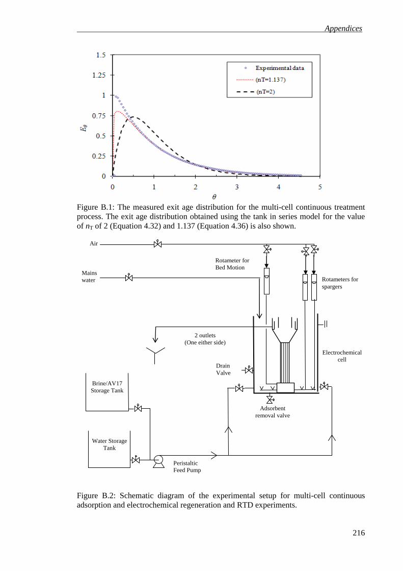
Appendices
216
Figure B.1: The measured exit age distribution for the multi-cell continuous treatment process. The exit age distribution obtained using the tank in series model for the value of nT of 2 (Equation 4.32) and 1.137 (Equation 4.36) is also shown.
Mains water
2 outlets (One either side)
Water Storage Tank
Drain Valve
Air
Peristaltic Feed Pump
Electrochemical cell
Rotameter for Bed Motion
Adsorbent removal valve
Rotameters for spargers
Brine/AV17 Storage Tank
Figure B.2: Schematic diagram of the experimental setup for multi-cell continuous adsorption and electrochemical regeneration and RTD experiments.

Appendices
217
Figure B.3: Reactor performance for adsorption and regeneration at various currents supplied in the Arvia multi-cell unit.

Appendices
218
Table B.3: Effect of initial concentration on the performance of the Arvia single-cell large unit for adsorption with electrochemical regeneration at feed flow rate of 0.6 L min−1.
Time Concentration (mg /L) Time Concentration (mg /L)
min Co=140 Co=153 Co=81 min Co=140 Co=153 Co=81
0 0 0 0 220 2650.6024 104.09639 1254.1733
10 120.48193 8.4337349 101.61126 230 2771.0843 103.51807 1247.2057
20 240.96386 24.096386 290.3179 240 2891.5663 103.37349 1245.4638
30 361.44578 37.228916 448.54115 250 3012.0482 105.54217 1271.5924
40 481.92771 47.710843 574.82944 260 3132.5301 105.54217 1271.5924
50 602.40964 57.108434 688.05342 270 3253.012 106.84337 1287.2696
60 722.89157 65.783133 792.56786 280 3373.494 106.98795 1289.0115
70 843.37349 71.566265 862.24416 290 3493.9759 106.98795 1289.0115
80 963.85542 79.518072 958.04906 300 3614.4578 106.48193 1282.9148
90 1084.3373 82.409639 992.88721 310 3734.9398 106.98795 1289.0115
100 1204.8193 85.301205 1027.7254 320 3855.4217 106.26506 1280.3019
110 1325.3012 88.192771 1062.5635 330 3975.9036 104.81928 1262.8829
120 1445.7831 91.084337 1097.4017 340 4096.3855 106.84337 1287.2696
130 1566.2651 93.975904 1132.2398 350 4216.8675 106.26506 1280.3019
140 1686.747 96.289157 1160.1103 360 4337.3494 105.54217 1271.5924
150 1807.2289 97.084337 1169.6908 370 4457.8313 106.98795 1289.0115
160 1927.7108 97.301205 1172.3037 380 4578.3133 106.98795 1289.0115
170 2048.1928 99.036145 1193.2066 390 4698.7952 106.91566 1288.1405
180 2168.6747 99.759036 1201.9161 400 4819.2771 106.26506 1280.3019
190 2289.1566 101.20482 1219.3352 410 4939.759 107.13253 1290.7534
200 2409.6386 102.6506 1236.7542 420 5060.241 107.42169 1294.2372
210 2530.1205 103.37349 1245.4638

Appendices
219
Table B.4: Effect of feed flow rate on the performance of the Arvia single-cell large unit for adsorption with electrochemical regeneration at initial concentration of around 100 mg L−1.
Time Concentration (mg/ L) Time
Concentration (mg/ L)
min Q=0.75 L/min
Q=0.25 L/min
Q=0.5 L/min min
Q=0.75 L/min
Q=0.25 L/min
Q=0.5 L/min
0 0 0 0 220 57.53 9.144 45
10 6.02 1.19 0.6 230 58.25 9.25 45.36
20 16.63 3.43 4.12 240 58.13 9.24 44.46
30 25.36 5.06 11.26 250 57.83 8.92 45.43
40 33.37 5.3 15.65 260 56.93 9.24 45.9
50 38.19 5.38 18.75 270 58.43 9.36 46.19
60 43.73 5.64 22.34 280 57.95 9.33 46.48
70 46.98 5.76 26.08 290 57.83 9.37 45.18
80 49.39 6.58 29.17 300 59.04 9.34 45.65
90 52.53 7.24 30.14 310 58.13 9.37 45.47
100 53.19 7.83 32.8 320 57.02 9.36 45.54
110 53.13 7.86 35.42 330 55 9.34 45.94
120 54.94 8.19 37.8 340 56.75 9.35 46.3
130 57.35 8.82 39.22 350 56.02 9.34 46.19
140 56.8 8.68 40.15 360 56.02 9.38 45.83
150 57.47 8.55 42.289 370 56.98 9.38 46.08
160 56.2 8.43 41.56 380 57.29 9.38 45.72
170 58.67 8.55 42.29 390 56.33 9.34 46.21
180 57.95 8.44 43.37 400 57.83 9.37 45.99
190 57.41 9.22 44.1 410 55.9 9.38 45.42
200 58.43 9.23 44.10# 420 56.44 9.37 46.14
210 58.07 9.24 44.82

Appendices
220
Table B.5: Reactor performance for adsorption with no regeneration (no current supplied) at feed flow rate of 0.75 L min−1 and feed concentration of around 107 mg L−1 in the Arvia single cell large unit.
Time Concentration Time Concentration Time Concentration
min mg / L min mg / L min mg / L
0 0 170 99.85 340 106.82
10 10.92 180 100.06 350 106.77
20 20.41 190 100.72 360 107.06
30 29.33 200 102.17 370 106.95
40 35.48 210 102.65 380 107.018
50 46.89 220 104.15 390 107.01
60 57.62 230 105.18 400 107.02
70 65.19 240 105.6 410 106.14
80 70.6 250 105.67 420 106.98
90 77.03 260 105.8 430 107.08
100 82.53 270 105.83 440 107.32
110 86.26 280 105.83 450 106.93
120 89.58 290 106.02 460 106.93
130 92.47 300 106.71 470 107.27
140 94.4 310 106.82 480 105
150 96.2 320 106.86
160 98.49 330 106.81
Table B.6: Reactor performance in the absence of adsorbent at feed flow rate of 0.75 L min−1 and feed concentration of 27 mg L−1 in the Arvia single cell large unit.
Time Concentration Time Concentration Time Concentration Time Concentration
min mg / L min mg / L min mg / L min mg / L
0 0.00 70 19.31 160 25.25 300 26.61
5 1.05 75 19.90 170 25.61 310 26.63
10 3.12 80 20.28 180 25.81 320 26.57
15 5.46 85 20.96 190 25.84 330 26.77
20 7.27 90 21.45 200 25.87 340 27.17
25 9.19 95 21.92 210 25.99 350 27.28
30 10.92 100 22.29 220 26.30 360 27.33
35 12.27 105 22.57 230 26.70 370 27.27
40 13.57 110 23.11 240 26.51 380 26.45
45 14.58 115 23.35 250 26.34 390 26.90
50 15.75 120 23.41 260 26.33 400 27.06
55 16.61 130 24.00 270 26.58 410 27.14
60 17.81 140 24.65 280 26.41 420 27.37
65 18.46 150 25.06 290 26.58 430 27.37

Appendices
221
Table B.7: Nozzle configuration and air flow rates for the adsorbent circulation experiments.
Test No. Air flow rate (L/min) Total Qair (both side)
I1 I2 I3 I4 I5 I6 L / min
1 0 0.5 3 4 4 4 31
2 0 1 2.5 4 4 4 31
3 0 2 1.5 4 4 4 31
4 0.5 1 2 4 4 4 31
5 0.5 1 2 6 6 6 43
6 0 0.5 2 8 5 6 43
7 0 1.5 3 2 6 6 37
8 0 2 1 2 2 2 18
9 0.5 1 2 2 2 2 19
Table B.8: Effect of water flow rate on the bed velocity in the Arvia single cell large unit.
Water flow rate (L / min) Test No. 0.25 0.5 0.6 0.75
Bed Velocity (cm / s)
1 0.04 0.04 0.05 0.04 0.05 0.05 0.05 0.05 0.05 0.06 0.05 0.06
2 0.09 0.09 0.1 0.1 0.1 0.89 0.1 0.12 0.1 0.1 0.12 0.11
3 0.12 0.12 0.13 0.12 0.12 0.12 0.13 0.13 0.14 0.13 0.14 0.14
Table B.9: Standard deviations for the experimental data are shown in Table B.8.
Water flow rate (L / min)
Test No. 0.25 0.5 0.6 0.75
Standard Deviation (SD)
1 0.003034 0.002936 0.0019 0.002646
2 0.004016 0.456165 0.010801 0.010786
3 0.005108 0.001882 0.003376 0.003215
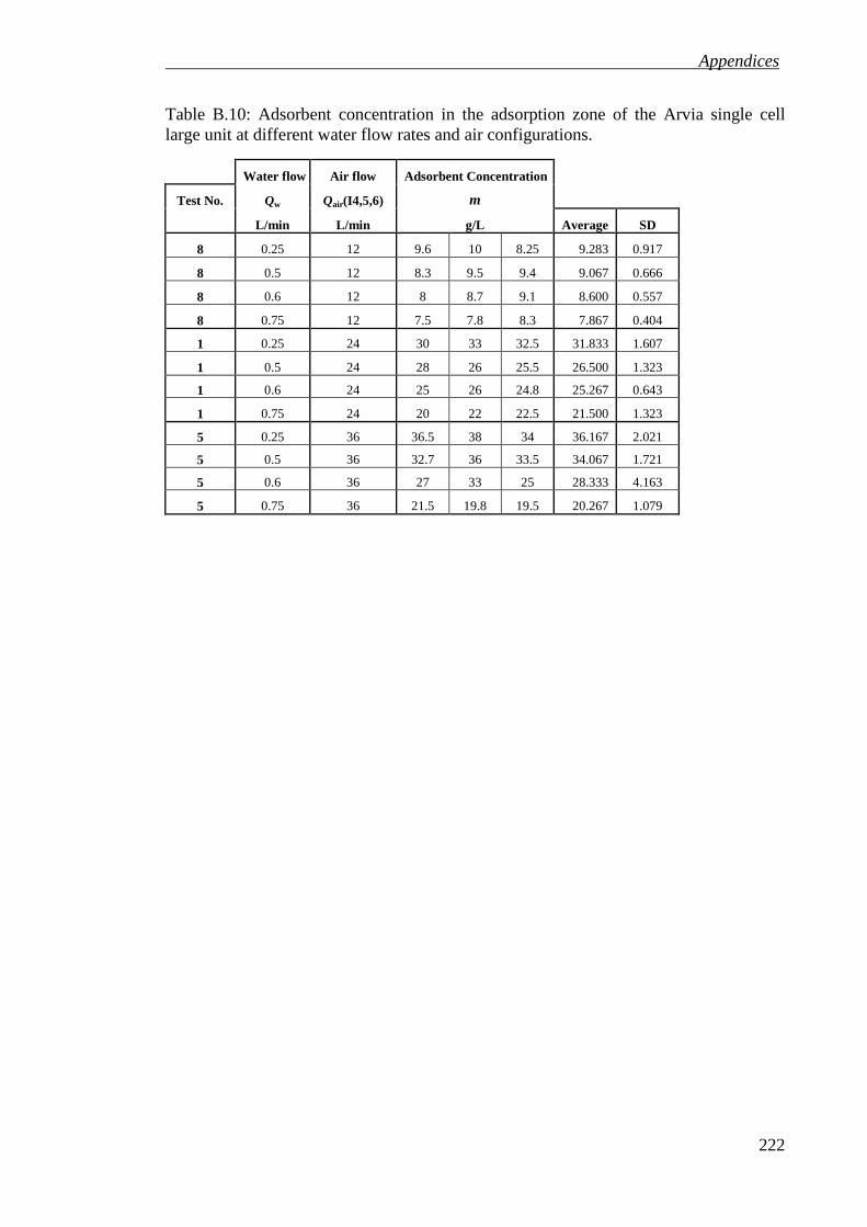
Appendices
222
Table B.10: Adsorbent concentration in the adsorption zone of the Arvia single cell large unit at different water flow rates and air configurations.
Water flow Air flow Adsorbent Concentration
Test No. Qw Qair(I4,5,6) m
L/min L/min g/L Average SD
8 0.25 12 9.6 10 8.25 9.283 0.917
8 0.5 12 8.3 9.5 9.4 9.067 0.666
8 0.6 12 8 8.7 9.1 8.600 0.557
8 0.75 12 7.5 7.8 8.3 7.867 0.404
1 0.25 24 30 33 32.5 31.833 1.607
1 0.5 24 28 26 25.5 26.500 1.323
1 0.6 24 25 26 24.8 25.267 0.643
1 0.75 24 20 22 22.5 21.500 1.323
5 0.25 36 36.5 38 34 36.167 2.021
5 0.5 36 32.7 36 33.5 34.067 1.721
5 0.6 36 27 33 25 28.333 4.163
5 0.75 36 21.5 19.8 19.5 20.267 1.079

Appendices
223
APPENDIX C
HYDROGEN PRODUCTION CALCULATION FOR THE SINGLE CELL PROCESS Hydrogen generated at the cathode and the amount of hydrogen in a single cathode
electrode can be calculated as follow:
From electrochemical regeneration of adsorbent in the batch cell, we found the optimum
current density is 7 mA cm−2.
Area of electrode (anode) = 60 x 12 cm = 720 cm2
Therefore, the optimum current used = 7 x 720 = 5040 mA = 5 A.
Maximum charge passed (from Chapter 3) = I x t = 15 C s−1.
From Faraday's Law, mole of electrons passed per second is:
=
(C.1)
where F = 96487 C mol−1 is the faraday constant.
Z = is the valence number of ions of the substance (electrons transferred per ion).
Hydrogen has been produced at the cathode as follow:
2 + 2 → ↑ (C.2)
The number of electrons transferred per ion (Z) = 2. Thus, Equation (C.1) becomes:
= 1596487 1
2 = 7.773 × 10" #$% &
General ideal gas law,
' ( = ) * (C.3)
At standard temperature and pressure, Equation (C.3)
= 1 #$% = '()* = +1 ,-#.(
82.06 × 10/ #0. ,-##$%. 1 × 2731
V = 22.402 L
Therefore, the production rate of hydrogen gas = (7.773x10⁻⁵ mol s−1) x (22.402 L)
= 1.742 x 10⁻³ L s−1 (0.006271 m3 h−1)
The volume of the vent cell = 68.04 m3
Volume exchanged per hour = (30 x 100%) x 68.04 = 2041.2 m3 (without recycle)

Appendices
224
Thus, the percentage of hydrogen in the air = (0.006271 / 2041.1) x 100 = 0.00031%
This percentage is below the 4% explosive limit for hydrogen (Lewis, 2004).
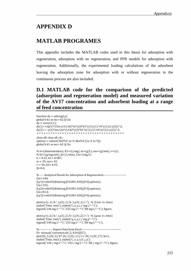
Appendices
225
APPENDIX D
MATLAB PROGRAMES
This appendix includes the MATLAB codes used in this thesis for adsorption with
regeneration, adsorption with no regeneration, and PFR models for adsorption with
regeneration. Additionally, the experimental loading calculations of the adsorbent
leaving the adsorption zone for adsorption with or without regeneration in the
continuous process are also included.
D.1 MATLAB code for the comparison of the predicted (adsorption and regeneration model) and measured variation of the AV17 concentration and adsorbent loading at a range of feed concentration function dy = adsreg+t,y. global b k1 m mo v k2 Q Cin dy = zeros+2,1.; dy+1. =+Q/v.*+Cin-y+1..-k2*m*+++b*k1*y+1../+1+b*y+1...-y+2..^2; dy+2. = -y+2.*mo/+m*v.+k2*+++b*k1*y+1../+1+b*y+1...-y+2..^2; ************************************** close all; clear all ;clc; options = odeset+'RelTol',1e-9,'AbsTol',[1e-9 1e-9].; global b k1 m mo v k2 Q Cin % b=+dimensionless., K1=+L/mg., m=+g/L., mo=+g/min., v=+L., % k2=+g/mg.min., Q=+L/min., Cin=+mg/L. b = 0.31; k1= 0.987; m = 25; mo= 42; v = 36; k2= 0.41; Q=0.6; % ---- Analytical Result for Adsorption & Regeneration ----------------------- Cin=140; [t,y1]=ode45+@adsreg,[0:0.001:420],[0 0],options.; Cin=153; [t,y2]=ode45+@adsreg,[0:0.001:420],[0 0],options.; Cin=81.4; [t,y3]=ode45+@adsreg,[0:0.001:420],[0 0],options.; plot+t,y1+:,1.,'k-', t,y2+:,1.,'b-',t,y3+:,1.,'r-'.; % +Cout. vs. time. xlabel+'Time /min'.; ylabel+'C_o_u_t / mg L^-^1'.; legend+'140 mg L^-^1','153 mg L^-^1','80 mg L^-^1'.; figure; plot+t,y1+:,2.,'k-', t,y2+:,2.,'b-',t,y3+:,2.,'r-'.; % +qout. vs. time. xlabel+'Time /min'.; ylabel+'q_o_u_t / mg g^-^1'.; legend+'140 mg L^-^1','153 mg L^-^1','80 mg L^-^1'.; %-------------- Export Data from Excel ---------------------------------------- D= xlsread+'currenton.xls',2,'A10:Q52'.; plot+D+:,1.,D+:,5.,'b*',D+:,1.,D+:,11.,'r+',D+:,1.,D+:,17.,'ko'.; xlabel+'Time /min'.; ylabel+'C_o_u_t/C_i_n'.; legend+'140 / mg L^-^1','153 / mg L^-^1','80 / mg L^-^1'.; figure;
Appendices
226
plot+D+:,1.,D+:,4.,'b*',D+:,1.,D+:,10.,'ko',D+:,1.,D+:,16.,'r+'.; xlabel+'Time /min'.; ylabel+'C_o_u_t / mg L^-^1'.; legend+'140 / mg L^-^1','153 / mg L^-^1','80 / mg L^-^1'.;figure; %---------- Calculate qout exp. +Range Kutta method. -------------------- i=length+D+:,1..; j=length+D+:,4..; h=10; for dd=+2:i. dt+dd-1.=D+dd,1.-D++dd-1.,1.; end Cin=140; for j=1:length+D+:,1..-1; qout_exp1+1.=0; G1=Q*+Cin-D+j,4../+m*v.-+mo/+m*v..*qout_exp1+j.-+D++j+1.,4.-D+j,4../+dt+j.*m.; G2=Q*+Cin-D+j,4../+m*v.-+mo/+m*v..*+qout_exp1+j.++0.5*h*G1..-+D++j+1.,4.-D+j,4../+dt+j.*m.; G3=Q*+Cin-D+j,4../+m*v.-+mo/+m*v..*+qout_exp1+j.++0.5*h*G2..-+D++j+1.,4.-D+j,4../+dt+j.*m.; G4=Q*+Cin-D+j,4../+m*v.-+mo/+m*v..*+qout_exp1+j.++h*G3..-+D++j+1.,4.-D+j,4../+dt+j.*m.; qout_exp1+j+1.=qout_exp1+j.++h/6.*+G1+2*G2+2*G3+G4.; end qout_exp1; Cin=153; j=length+D+:,10..; for j=1:length+D+:,1..-1; qout_exp2+1.=0; G1=Q*+Cin-D+j,10../+m*v.-+mo/+m*v..*qout_exp2+j.-+D++j+1.,10.-D+j,10../+dt+j.*m.; G2=Q*+Cin-D+j,10../+m*v.-+mo/+m*v..*+qout_exp2+j.++0.5*h*G1..-+D++j+1.,10.-D+j,10../+dt+j.*m.; G3=Q*+Cin-D+j,10../+m*v.-+mo/+m*v..*+qout_exp2+j.++0.5*h*G2..-+D++j+1.,10.-D+j,10../+dt+j.*m.; G4=Q*+Cin-D+j,10../+m*v.-+mo/+m*v..*+qout_exp2+j.++h*G3..-+D++j+1.,10.-D+j,10../+dt+j.*m.; qout_exp2+j+1.=qout_exp2+j.++h/6.*+G1+2*G2+2*G3+G4.; end qout_exp2; Cin=81.4; j=length+D+:,16..; for j=1:length+D+:,1..-1; qout_exp3+1.=0; G1=Q*+Cin-D+j,16../+m*v.-+mo/+m*v..*qout_exp3+j.-+D++j+1.,16.-D+j,16../+dt+j.*m.; G2=Q*+Cin-D+j,16../+m*v.-+mo/+m*v..*+qout_exp3+j.++0.5*h*G1..-+D++j+1.,16.-D+j,16../+dt+j.*m.; G3=Q*+Cin-D+j,16../+m*v.-+mo/+m*v..*+qout_exp3+j.++0.5*h*G2..-+D++j+1.,16.-D+j,16../+dt+j.*m.; G4=Q*+Cin-D+j,16../+m*v.-+mo/+m*v..*+qout_exp3+j.++h*G3..-+D++j+1.,16.-D+j,16../+dt+j.*m.; qout_exp3+j+1.=qout_exp3+j.++h/6.*+G1+2*G2+2*G3+G4.; end qout_exp3; plot+D+:,1.,qout_exp1,'b*',D+:,1.,qout_exp2,'ko',D+:,1.,qout_exp3,'r+'.; xlabel+'Time / min'.; ylabel+'q_o_u_t / mg g^-^1'.; legend+'140 / mg L^-^1','153 / mg L^-^1','80 / mg L^-^1'.;figure; plot+D+:,1.,qout_exp1,'b*',t,y1+:,2.,'b-',D+:,1.,qout_exp2,'ko',t,y2+:,2.,'k-',D+:,1.,qout_exp3,'r+',t,y3+:,2.,'r-'.; %t vs. q exp. and model xlabel+'Time / min'.; ylabel+'q_o_u_t / mg g^-^1'.; legend+'Experiment data 140 / mg L^-^1','Model 140 / mg L^-^1','Experiment data 153 / mg L^-^1','Model 153 / mg L^-^1','Experiment data 80 / mg L^-^1','Model 80 / mg L^-^1'.; figure; plot+D+:,1.,D+:,4.,'b*',t,y1+:,1.,'b-',D+:,1.,D+:,10.,'ko',t,y2+:,1.,'k-',D+:,1.,D+:,16.,'r+',t,y3+:,1.,'r-'.; % t vs Cout model and exp. xlabel+'Time /min'.; ylabel+'C_o_u_t / mg L^-^1'.; legend+'Experiment data 140 / mg L^-^1','Model 140 / mg L^-^1','Experiment data 153 / mg L^-^1','Model 153 / mg L^-^1','Experiment data 80 / mg L^-^1','Model 80 / mg L^-^1'.;

Appendices
227
D.2 MATLAB code for the comparison of the predicted (adsorption and regeneration model) and measured variation of the AV17 concentration and adsorbent loading at a range of feed flow rate function dy = adsreg+t,y. global b k1 m mo v k2 Q Cin dy = zeros+2,1.; dy+1. =+Q/v.*+Cin-y+1..-k2*m*+++b*k1*y+1../+1+b*y+1...-y+2..^2; dy+2. = -y+2.*mo/+m*v.+k2*+++b*k1*y+1../+1+b*y+1...-y+2..^2; ************************************** close all; clear all ;clc; options = odeset+'RelTol',1e-9,'AbsTol',[1e-9 1e-9].; global b k1 m mo v k2 Q Cin %----------------- Units ----------------- % b=+dimensionless., K1=+L/mg., m=+g/L., mo=+g/min., v=+L., k2=+g/mg.min., Q=+L/min., Cin=+mg/L. b = 0.31 ; k1= 0.987 ; v = 36 ; k2= 0.41 ; Cin=99; % ---- Analytical Result for Adsorption & Regeneration --------- m=24; mo=50; Q=0.75; [t,y1]=ode45+@adsreg,[0:0.001:420],[0 0],options.; m=27; mo=41; Q=0.5; [t,y2]=ode45+@adsreg,[0:0.001:420],[0 0],options.; m=30; mo=40.5; Q=0.25; [t,y3]=ode45+@adsreg,[0:0.001:420],[0 0],options.; plot+t,y1+:,1.,'k-', t,y2+:,1.,'b-',t,y3+:,1.,'r-'.; % +Cout vs. time. xlabel+'Time /min'.; ylabel+'C_o_u_t / mg L^-^1'.; legend+'140 mg L^-^1','153 mg L^-^1','80 mg L^-^1'.; figure; plot+t,y1+:,2.,'k-', t,y2+:,2.,'b-',t,y3+:,2.,'r-'.; % +qout vs. time. xlabel+'Time /min'.; ylabel+'q_o_u_t / mg g^-^1'.; legend+'140 mg L^-^1','153 mg L^-^1','80 mg L^-^1'.; %-------------- Export Data from Excel--------------------- D= xlsread+'currenton.xls',1,'A10:Q52'.; plot+D+:,1.,D+:,5.,'b*',D+:,1.,D+:,17.,'r+',D+:,1.,D+:,11.,'ko'.; xlabel+'Time /min'.; ylabel+'C_o_u_t/C_i_n'.; legend+'0.75 / L min^-^1','0.5 / L min^-^1','0.25 / L min^-^1'.; figure; plot+D+:,1.,D+:,4.,'b*',D+:,1.,D+:,16.,'r+',D+:,1.,D+:,10.,'ko'.; xlabel+'Time /min'.; ylabel+'C_o_u_t / mg L^-^1'.; legend+'0.75 / L min^-^1','0.5 / L min^-^1','0.25 / L min^-^1'.;figure; %---------- Calculate qout exp. +Range Kutta method. ---------- i=length+D+:,1..; j=length+D+:,4..; h=10; for dd=+2:i. dt+dd-1.=D+dd,1.-D++dd-1.,1.; end Q=0.75;

Appendices
228
m=20; mo=53; j=length+D+:,4..; for j=1:length+D+:,1..-1; qout_exp1+1.=0; G1=Q*+Cin-D+j,4../+m*v.-+mo/+m*v..*qout_exp1+j.-+D++j+1.,4.-D+j,4../+dt+j.*m.; G2=Q*+Cin-D+j,4../+m*v.-+mo/+m*v..*+qout_exp1+j.++0.5*h*G1..-+D++j+1.,4.-D+j,4../+dt+j.*m.; G3=Q*+Cin-D+j,4../+m*v.-+mo/+m*v..*+qout_exp1+j.++0.5*h*G2..-+D++j+1.,4.-D+j,4../+dt+j.*m.; G4=Q*+Cin-D+j,4../+m*v.-+mo/+m*v..*+qout_exp1+j.++h*G3..-+D++j+1.,4.-D+j,4../+dt+j.*m.; qout_exp1+j+1.=qout_exp1+j.++h/6.*+G1+2*G2+2*G3+G4.; end qout_exp1; Q=0.5; m=27; mo=41; j=length+D+:,16..; for j=1:length+D+:,1..-1; qout_exp2+1.=0; G1=Q*+Cin-D+j,16../+m*v.-+mo/+m*v..*qout_exp2+j.-+D++j+1.,16.-D+j,16../+dt+j.*m.; G2=Q*+Cin-D+j,16../+m*v.-+mo/+m*v..*+qout_exp2+j.++0.5*h*G1..-+D++j+1.,16.-D+j,16../+dt+j.*m.; G3=Q*+Cin-D+j,16../+m*v.-+mo/+m*v..*+qout_exp2+j.++0.5*h*G2..-+D++j+1.,16.-D+j,16../+dt+j.*m.; G4=Q*+Cin-D+j,16../+m*v.-+mo/+m*v..*+qout_exp2+j.++h*G3..-+D++j+1.,16.-D+j,16../+dt+j.*m.; qout_exp2+j+1.=qout_exp2+j.++h/6.*+G1+2*G2+2*G3+G4.; end qout_exp2; Q=0.25; m=30; mo=40.5; j=length+D+:,10..; for j=1:length+D+:,1..-1; qout_exp3+1.=0; G1=Q*+Cin-D+j,10../+m*v.-+mo/+m*v..*qout_exp3+j.-+D++j+1.,10.-D+j,10../+dt+j.*m.; G2=Q*+Cin-D+j,10../+m*v.-+mo/+m*v..*+qout_exp3+j.++0.5*h*G1..-+D++j+1.,10.-D+j,10../+dt+j.*m.; G3=Q*+Cin-D+j,10../+m*v.-+mo/+m*v..*+qout_exp3+j.++0.5*h*G2..-+D++j+1.,10.-D+j,10../+dt+j.*m.; G4=Q*+Cin-D+j,10../+m*v.-+mo/+m*v..*+qout_exp3+j.++h*G3..-+D++j+1.,10.-D+j,10../+dt+j.*m.; qout_exp3+j+1.=qout_exp3+j.++h/6.*+G1+2*G2+2*G3+G4.; end qout_exp3; plot+D+:,1.,qout_exp1,'b*',D+:,1.,qout_exp2,'r+',D+:,1.,qout_exp3,'ko'.; xlabel+'Time / min'.; ylabel+'q_o_u_t / mg g^-^1'.; legend+'0.75 / L min^-^1','0.5 / L min^-^1','0.25 / L min^-^1'.; figure; plot+D+:,1.,qout_exp1,'b*',t,y1+:,2.,'b-',D+:,1.,qout_exp2,'r+',t,y2+:,2.,'r-',D+:,1.,qout_exp3,'ko',t,y3+:,2.,'k-'.; xlabel+'Time / min'.; ylabel+'q_o_u_t / mg g^-^1'.; legend+'Experiemnt 0.75 / L min^-^1','Model 0.75 / mg L^-^1','Experiment 0.5 / L min^-^1','Model 0.5 / mg L^-^1','Experiment 0.25 / L min^-^1','Model 0.25 / L min^-^1'.; figure; plot+D+:,1.,D+:,4.,'b*',t,y1+:,1.,'b-',D+:,1.,D+:,10.,'ko',t,y3+:,1.,'k-',D+:,1.,D+:,16.,'r+',t,y2+:,1.,'r-'.; xlabel+'Time /min'.; ylabel+'C_o_u_t / mg L^-^1'.; legend+'Experiment data 0.75 / L min^-^1','Model 0.75 / L min^-^1','Experiment data 0.25 / L min^-^1','Model 0.25 / L min^-^1','Experiment data 0.5 / L min^-^1','Model 0.5 / L min^-^1'.;
Appendices
229
D.3 MATLAB Code for comparison of the predicted (adsorption with no regeneration model) and measured variation of the AV17 concentration and adsorbent loading close all; clear all; clc; options = odeset+'RelTol',1e-9,'AbsTol',[1e-9 1e-9].; global b k1 m mo v k2 Q Cin cout+1.=0; qout+1.=0; % initial condition t+1.=0; % initial time condition b=0.31; k1=0.987; m=24; v=36; k2=0.41; Q=0.75; Cin=106.7; n=1500; mo=50; % ------------- Euler Methods ------------------------------- tc=n/mo; disp+tc.; nc=input+'number of time steps up to tc = '. h=tc/nc; tmax = input +'tmax = '. nmax=tmax/h; for i = 1:nmax t+i+1.=t+i.+h; if +i <=nc. qin+i.=0; else qin+i.=qout+i-nc.; end cold=cout+i.; qold=qout+i.; fac=b*k1*cold/+1+b*cold.-qold; coutd=+Q/v.*+Cin-cold.-k2*m*fac*fac; %+dCout/dt.Euler method qoutd=+mo/+m*v..*+qin+i.-qold.+k2*fac*fac; % +dqout/dt.Euler method cout+i+1.=cout+i.+h*coutd; qout+i+1.=qout+i.+h*qoutd; qin+i+1.=qin+i.; end % ------------- Experiment Data for Adsorption----------------------------- tt=[0 10 20 30 40 50 60 70 80 90 100 110 120 130 140 150 160 170 180 190 200 210 220 230 240 250 260 270 280 290 300 310 320 330 340 350 360 370 380 390 400 410 420 430 440 450 460 470 480]; Cout=0.22*[0 49.5 92.56 132.9 160.9 212.62 261.32 295.65 320 349.3 374.32 391 406.28 419.2 428 436.24 446.7 452.8 453.2 456.72 463.56 465.83 472.57 477.12 479 479.3 479.84 480 480.2 481 484 484.5 484.67 484.43 484 484 484.3 485.6 485.05 485.34 485.68 485.43 481.42 485.23 485.68 486.77 484.86 484.51 486.23]; %-------------- calculates qout exp. ---------------------- i=length+tt.; for dd=+2:i.; dtt+dd-1.=tt+dd.-tt+dd-1.; end he=input+'interval time of experiment he='. nce=tc/he; nmaxe=tmax/he; qout1+1.=0; Cout+1.=0; for j=1:nmaxe if +j<=nce. qin1+j.=0; else qin1+j.=qout1+j-nce.;

Appendices
230
end qoutd1=Q*+Cin-Cout+j../+m*v.-+mo/+m*v..*qout1+j.++mo/+m*v..*qin1+j.-++Cout+j+1.-Cout+j../+dtt+j.*m..; qout1+j+1.=qout1+j.+he*qoutd1; end plot+t,qout.; xlabel+'Time / min'.; ylabel+'q_o_u_t / mg g^-^1.'.; figure; %--------------- Dilution Effect ------------------------ Cout_dilution=Cin*+1-exp+-tt*Q/v..; plot+t,cout,'k-',tt,Cout,'ro',tt,Cout_dilution,'b--'.; legend+'Adsorption with bed circulation model','Experimental data','Dilution model +k_2 = 0.'.; xlabel+'Time / min'.; ylabel+'C_o_u_t / mg L^-^1'.; figure; plot+t,qout,'k-',t,qin,'r--'.; xlabel+'Time / min'.;ylabel+'q / mg g^-^1'.; legend+'q_o_u_t','q_i_n'.; figure; plot+tt,qout1,'b*'.; xlabel+'Time / min'.;ylabel+'q_o_u_t / mg g^-^1'.;figure; plot +tt,qout1,'b*',t,qout,'k-'.; xlabel+'Time / min'.; ylabel+'q_o_u_t / mg g^-^1'.; legend+'Experimental data','Adsorption model'.; figure; plot +tt,Cout,'ro'.; xlabel+'Time / min'.; ylabel+'C_o_u_t / mg L^-^1'.; figure; plot +tt,Cout/Cin,'ro'.; xlabel+'Time / min'.; ylabel+'C_o_u_t / C_i_n'.; figure; k2=0.7; cout2+1.=0; qout2+1.=0; for i = 1:nmax t+i+1.=t+i.+h; if +i <=nc. qin2+i.=0; else qin2+i.=qout2+i-nc.; end cold2=cout2+i.; qold2=qout2+i.; fac=b*k1*cold2/+1+b*cold2.-qold2; coutd2=+Q/v.*+Cin-cold2.-k2*m*fac*fac; %+dCout/dt.Euler method qoutd2=+mo/+m*v..*+qin2+i.-qold2.+k2*fac*fac; % +dqout/dt.Euler method cout2+i+1.=cout2+i.+h*coutd2; qout2+i+1.=qout2+i.+h*qoutd2; qin2+i+1.=qin2+i.; end plot +tt,qout1,'b*',t,qout,'k-',t,qout2,'r-'.; xlabel+'Time / min'.; ylabel+'q_o_u_t / mg g^-^1'.; legend+'Experimental data','Adsorption model','Adsorption model at k_2=0.7'.; ******************************************************* m1=qout+1:333:16001.; % taking 49 point only m2=qout2+1:333:16001.; % taking 49 point only R1=sqrt+mean+m1.*qout1.. % correlation for model 1 where +R1.^2=mean+m1.*qout1. R2=sqrt+mean+m2.*qout1.. % correlation for model 2 where +R2.^2=mean+m2.*qout1.

Appendices
231
D.4 MATLAB code for calculation of the maximum loading for AV17 in adsorption with no regeneration process close all; clear all ;clc; t = [ 0 10 20 30 40 50 60 70 80 90 100 110 120 130 140 150 160 170 180 190 200 210 220 230 240 250 260 270 280 290 300 310 320 330 340 350 360 370 380 390 400 410 420 430 440 450 460 470 480]; Cout =0.22*[0 49.5 92.56 132.9 160.9 212.62 261.32 295.65 320 349.3 374.32 391 406.28 419.2 428 436.24 446.7 452.8 453.2 456.72 463.56 465.83 472.57 477.12 479 479.3 479.84 480 480.2 481 484 484.5 484.67 484.43 484 484 484.3 485.6 485.05 485.34 485.68 485.43 481.42 485.23 485.68 486.77 484.86 484.51 486.23]; % ------------ Units -------------------------------------------- %------- M +g., V+L., Cin +mg/L., Q +L/min.----------- Cin = 107; M=4000; V=36; Q = 0.75; i = length+t.; j=length+Cout.; qout_exp2=zeros+1,i.; summatn=0; for dd=+2:i. dt+dd-1.=t+dd.-t+dd-1.; end for ff=+2:j. Strip=sum+++Cin-Cout+ff-1..++Cin-Cout+ff...*Q*dt+ff-1../+2*M.; summatn=summatn+Strip; qout_exp2+ff.=summatn-V/+2*M.*Cout+ff.; end qout_exp2; disp+qout_exp2+j..; plot+t,qout_exp2,'r*'.; xlabel+'Time / min'.; ylabel+'qout / mg.g-1'.; figure; plot+t,Cout,'k*'.; xlabel+'Time / min'.; ylabel+'Cout / mg.L-1'.;

Appendices
232
D.5 MATLAB Code for PFR model of adsorption with regeneration process close all; clear all; clc; qout+1.=0; % initial condition V+1.=0; % initial time condition b=0.31; k1=0.987; m=16.35; mo=43; Vout=40; k2=0.41; Q=1; Cin=100; %----------- Euler Method ------------------------------------ n=input+'number of volume steps up to Vout = '. h=Vout/n; Vmax = input +'Vmax = '. nmax=Vmax/h; for i = 1:nmax V+i+1.=V+i.+h; qold=qout+i.; fac=b*k1*+Cin-+mo/Q.*qold./+1+b*+Cin-+mo/Q.*qold..-qold; qoutd=+k2/Q.*fac*fac; % +dqout/dt.Euler method qout+i+1.=qout+i.+h*qoutd; end disp+qout+n..; % ------- Cout at V=Vout and at qout+n. -------------- Cout=Cin-+mo/Q.*qout+n.; disp+Cout.; plot+V,qout. xlabel+'V +L.'.; ylabel+'q_o_u_t /mg g^-^1'.; figure; Cout1=Cin-+mo/Q.*qout; plot+V,Cout1. xlabel+'V +L.'.; ylabel+'C_o_u_t /mg L^-^1'.;
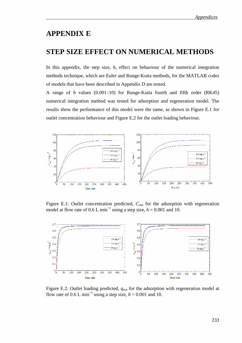
Appendices
233
APPENDIX E
STEP SIZE EFFECT ON NUMERICAL METHODS In this appendix, the step size, h, effect on behaviour of the numerical integration
methods technique, which are Euler and Runge-Kutta methods, for the MATLAB codes
of models that have been described in Appendix D are tested.
A range of h values (0.001–10) for Runge-Kutta fourth and fifth order (RK45)
numerical integration method was tested for adsorption and regeneration model. The
results show the performance of this model were the same, as shown in Figure E.1 for
outlet concentration behaviour and Figure E.2 for the outlet loading behaviour.
Figure E.1: Outlet concentration predicted, Cout for the adsorption with regeneration model at flow rate of 0.6 L min−1 using a step size, h = 0.001 and 10.
Figure E.2: Outlet loading predicted, qout for the adsorption with regeneration model at flow rate of 0.6 L min−1 using a step size, h = 0.001 and 10.
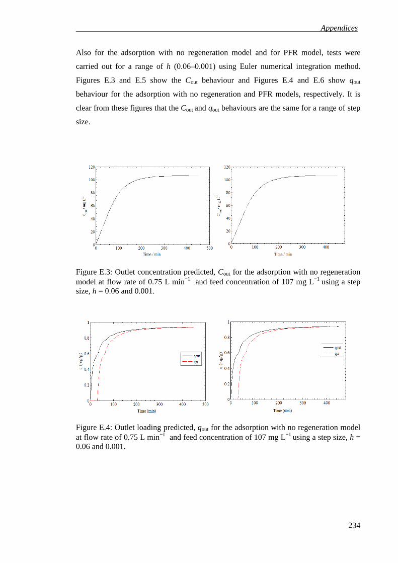
Appendices
234
Also for the adsorption with no regeneration model and for PFR model, tests were
carried out for a range of h (0.06–0.001) using Euler numerical integration method.
Figures E.3 and E.5 show the Cout behaviour and Figures E.4 and E.6 show qout
behaviour for the adsorption with no regeneration and PFR models, respectively. It is
clear from these figures that the Cout and qout behaviours are the same for a range of step
size.
Figure E.3: Outlet concentration predicted, Cout for the adsorption with no regeneration model at flow rate of 0.75 L min−1 and feed concentration of 107 mg L−1 using a step size, h = 0.06 and 0.001.
Figure E.4: Outlet loading predicted, qout for the adsorption with no regeneration model at flow rate of 0.75 L min−1 and feed concentration of 107 mg L−1 using a step size, h = 0.06 and 0.001.
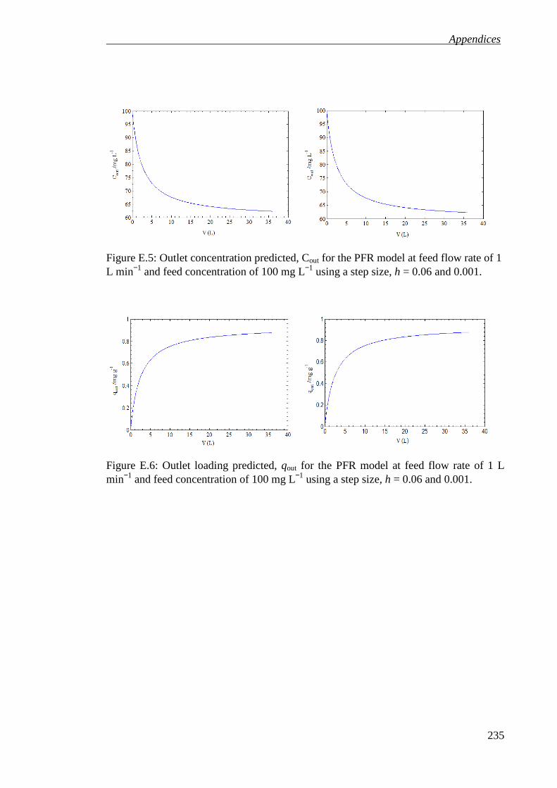
Appendices
235
Figure E.5: Outlet concentration predicted, Cout for the PFR model at feed flow rate of 1 L min−1 and feed concentration of 100 mg L−1 using a step size, h = 0.06 and 0.001.
Figure E.6: Outlet loading predicted, qout for the PFR model at feed flow rate of 1 L min−1 and feed concentration of 100 mg L−1 using a step size, h = 0.06 and 0.001.
Appendices
236
APPENDIX F
LIST OF PUBLICATIONS MOHAMMED, F. M., ROBERTS, E. P. L., HILL, A., CAMPEN, A. K. & BROWN, N. W. (2011) Continuous water treatment by adsorption and electrochemical regeneration. Water Research, 45, 3065-3074. MOHAMMED, F. M., ROBERTS, E. P. L., CAMPEN, A. K. & BROWN, N. W.(2010) Removal of dissolved organic contaminants by a continuous process using adsorption and electrochemical regeneration. EMChIE. Mechelen - Belgium.

Appendices
237
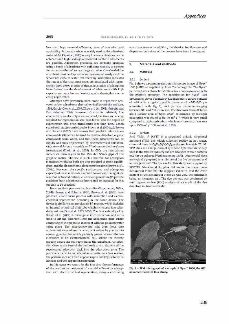
Appendices
238

Appendices
239

Appendices
240
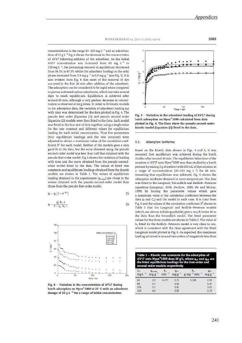
Appendices
241
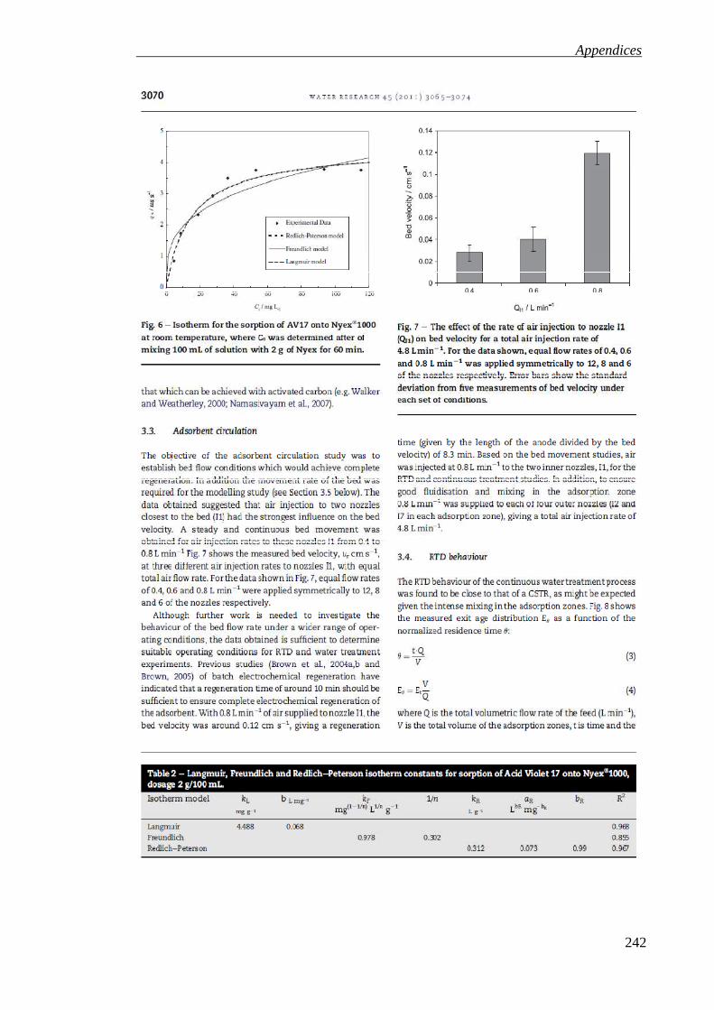
Appendices
242
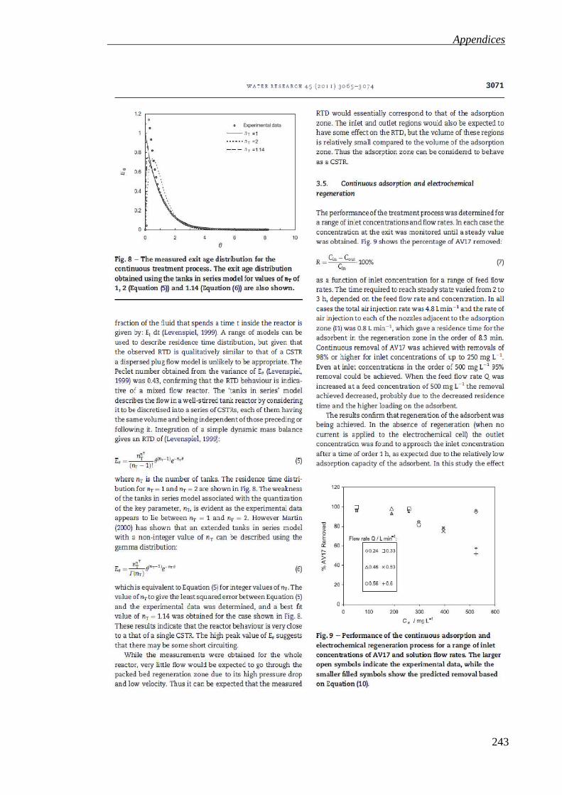
Appendices
243

Appendices
244

Appendices
245

Appendices
246
Appendices
247

Appendices
248
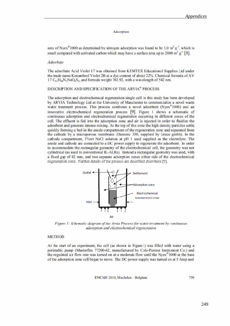
Appendices
249

Appendices
250

Appendices
251

Appendices
252
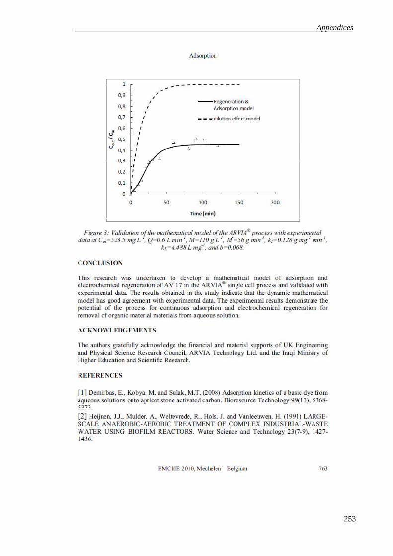
Appendices
253

Appendices
254