MODELING VOLTAGE IN BATTERY CELLS - Uppsala …ikaj/preprints/modvoltagebasic2.pdf · MODELING...

MODELING VOLTAGE IN BATTERY CELLS

UNDER DISCHARGE

INGEMAR KAJ AND VICTORIEN KONANE

Abstract. In this paper we review several approaches to mathematical modelingof simple battery cells and develop these ideas further with emphasis on chargerecovery and the response behavior of batteries to given external load. We focuson models which use few parameters and basic battery data, rather than detailedreaction and material characteristics of a specific battery cell chemistry, startingwith the coupled ODE linear dynamics of a kinetic battery model. We showthat a related system of PDE with Robin type boundary conditions arises in thelimiting regime of a spatial kinetic battery model, and provide a probabilisticrepresentation of the solution in terms of Brownian motion with drift reflectedat the boundaries on both sides of a finite interval. Moving on to nonlinearbattery models we consider a discrete time Markov chain with states representingnominal and remaining capacities of the battery. A nonlinear ODE appears in anatural scaling limit, which leads to a wider class of nonlinear ODE which can besolved explicitly and compared with the capacities obtained for the linear models.To indicate the potential use of the modeling we discuss briefly comparison ofdischarge profiles and effects on battery performance.

1. Introduction

The subject of this work is mathematical modeling of state-of-charge and voltagelevel in simple battery cells, such as a non-rechargeable 3 Volts Lithium coin battery.The goal is to understand the response of the battery, and ultimately to predictbattery lifetime, as capacity is consumed under a given discharge usage pattern.The main incentive for our work is the battery usage in Wireless Sensor Networksand similar Internet-of-Things systems. These networks consist of inter-connectedlow-cost nodes, equipped with basal sensors, computer, radio and a battery, expectedto run for many years under very low intensity loads and short dutycycles. Thereare no known methods or techniques providing a “battery-charge indicator” for suchsystems. A possible approach is progress on the battery life prediction problem. Inthis direction, our paper intends to cover some of the required modeling groundwork.Mathematical modeling of batteries has developed over several decades along with

the growth of new battery technologies and materials. Yet, there has been relativelylittle in-depth study of widely available, inexpensive coin cell batteries and on specialload characteristics including short load periods. Primarily, lithium and lithium-ionbattery models have been developed within electrochemical engineering.

1

2 INGEMAR KAJ AND VICTORIEN KONANE

Two recent survey and review works[8, 12] represent the state-of-art of modelingbased on the fundamental principles of electrochemistry, and emphasise the widerange of scales involved. The temporal and spatial scales of the physics and chem-istry of the battery range from macroscopic level all the way down to the atomisticlevel. The tutorial review by Landstorfer and Jacob[8] provides a framework ofnon-equilibrium thermodynamics as the foundation for studying the electrode, elec-trolyte and interface reactions in great detail. The review work by Ramadesigan etal.[12], summarizes the literature on such models and, in addition, brings a systemsengineering approach applied to Li-ion batteries. This type of model can be saidto begin with the pseudo-two-dimensional (P2D) model of Doyle et al.[5], whichleads to a coupled system of non-linear PDEs. More generally, coupled systems ofequations with complex boundary conditions are derived, which connect charge con-centrations with transport and kinetics of reactant species. Several approaches havebeen proposed to simplify the resulting sets of equations and allow for numericalcomputations, see e.g. [[15, 3]].Battery modeling based on a somewhat different mathematical approach in com-

parison to chemical engineering modeling have appeared in communication engineer-ing for computer science applications, see e.g. Jongerden and Haverkort[6]. Wherechemical engineering modeling typically begins with a detailed scheme of reactionsand mechanisms in the various phases and interfaces of the cell, these models viewthe battery as a generic device. The main focus of the modeling changes and isnow rather the response of the battery to external load. A typical purpose is loadscheduling to optimize battery utilization. Important aspects of battery behaviorfrom this point of view are the rate-capacity effect and charge recovery. Quoting[[14]]: The former refers to the fact that a lower discharge rate is more efficientthan a higher; more charge can be extracted from the battery before reaching a givencut-off value. The latter refers to the fact that an intermittent discharge is moreefficient than a continuous one. Because of these effects, different battery loads thatuse the same total charge do not result in the same device lifetime. The most basicof these methods use linear ODEs[9, 10] and gradually build complexity by usingPDEs and other means[11, 13, 6]. Battery models have seen very little exposure intraditional journals and publications typical for applied mathematics; one of a fewrecent exceptions is [[4]].Our conceptual approach in this work will be that of communications engineering

in the sense that we rely on the notion that a lithium coin cell is a generic devicesubject to some fundamental principles. Without ignoring or overly simplifying thecomplex mechanisms of modern batteries our main interest is to capture the essentialresponse of the battery to discharge. Hence we use only a few parameters and basicbattery data rather than detailed reaction coefficients and material characteristicsvalid for a specific type of battery cell chemistry.

MODELING BATTERY CELLS 3

Two important aspects of battery behavior that must be covered by the dynamicsof a mathematical model are internal resistance and the ability of a cell to recovercharge during operation. As for internal resistances along the interior circuit of abattery under load, the basic approach is that of constant voltage drop according toOhm’s law and more general versions often refer to an equivalent circuits approach.Charge recovery, believed to depend on a number of internal mechanisms of whichconvection, migration, diffusion and charge-transfer are discussed in some detailbelow, is the main theme of this article.The mathematical approach of the paper has its roots in linear dynamics starting

from the so called kinetic battery model[9, 10], which describes the joint evolutionof available charge and bound charge over time. Charge recovery in this frameworkconsists in the continuous transition of bound charge to available charge. As ob-served in [[6]] and further investigated in [[7]], more general spatial versions of thesemodels are related to a class of second order diffusion equations with Robin typeboundary conditions introduced in [[11, 13]].In Section 2, following preliminaries on capacities, recovery mechanisms and dis-

charge profiles, we introduce the basic kinetic battery model and discuss a variation.Then we set up an extended version of the spatial kinetic battery model with a finitenumber of serial compartments, derive the spatially continuous limiting PDE, andgive a probabilistic representation of the solution of the PDE in terms of Brownianmotion with drift reflected at the boundaries on both sides of a finite interval. Thesolution represents the capacity storage of a battery and these tools again allow usto study the balance of nominal and remaining stored capacity. Section 3 is de-voted to the prospects of using alternative nonlinear models for similar purposes asthe linear models in Section 2. We begin with a discrete time Markov chain withnonlinear jump probabilities derived from a simplified charge transport scenario.By a scaling approximation we obtain in the limit a deterministic nonlinear ODE,with explicit solutions which, in principle, can be compared to those of the linearapproach. Indeed, with proper choice of nonlinear dynamics for charge recoverydue to transfer, diffusion and migration effects, we propose a somewhat wider classof nonlinear ODE of potential use for battery modeling. As a consequence, it ispossible to study performance measures such as battery life, delivered capacity andgain, and to compare and optimize the performance of batteries.

2. Linear Battery Models

2.1. Nominal capacity. We consider a non-rechargeable battery cell consisting oftwo electrodes, anode and cathode, linked by an electrolyte. The cell contains acertain amount of chemically reactive material which is converted into electricalenergy by an oxidation reaction at the anode. Primary lithium batteries have alithium anode and may have soluble or solid electrolytes and cathodes. The mass


of material involved in the battery reaction yields a higher concentration of elec-trons at the anode, and hence by Faraday’s first law the transfer of a proportionalquantity of electrical charge. This determines a terminal voltage between the pairof electrodes. By closing a wired circuit between the terminals a current of electronswill start moving through the wire from anode to cathode where they react witha positively charged reactant, manifesting the ability of the battery to drive elec-tric current. The intensity of the current depends on the total resistance along thewire. Inside the battery the movement of charge-carriers forms a corresponding ioniccurrent, which is controlled by a variety of mechanisms, among them migration ofions, diffusion of reactant species, and charge-transfer reaction. Migration is gener-ated by an electric potential gradient (electric field) and convective diffusion by theconcentration gradient. Conductivity arises from the combination of migration anddiffusion. Charge-transfer reactions take place when migrating ions are transferedfrom the electrolyte bulk through the anode surface.It is sometimes helpful to keep track of proper units. The battery has a given

voltage E0 in volts [V] and a theoretical capacity T in ampere hours [Ah], repre-senting the entire storage of chemically reactive material in the cell. We write N[Ah] for the nominal capacity of a fully loaded cell, where N ≤ T . This is theamount of electric charge which is delivered if the cell is put under constant, highload and drained until it holds no more energy. Measuring time t in hours [h] wewrite Λ(t) for the consumed capacity [Ah] and v(t) = T − Λ(t) for the remainingcapacity [Ah], at time t. Here, Λ = (Λ(t))t≥0 is an increasing function, typicallycontinuous with the slope representing intensity of the current. It is also plausibleto let the discharge function have jumps to be interpreted as spikes of charge unitsbeing released pointwise to the device driven by the battery. As an additional levelof generality it is straigtforward to consider Λ defined on a probability space andsubject to a suitable distributional law of a random process. The instantaneous dis-charge current [A] at t is the derivative Λ′(t) = limh→ h−1Λ(t + h) and the averagedischarge current [A] is the quantity λ = limt→∞ t−1Λ(t), assuming this limit exists.We are interested in the behavior of the battery cell when exposed to the accu-

mulated discharge process Λ, in particular regarding

u(t) = nominal capacity [Ah] at time t, u(0) = N

u(t) = u(t)/N = state of charge at time t, u(0) = 1

E(t) = voltage [V] at time t, E(0) = E0.

While there is no obvious method of observing state-of-charge empirically, voltageis accesible to measurements at least in principle. To describe typical voltage, weimagine that a fully charged battery at time t = 0 is connected to a closed circuitat constant discharge current δ = Λ′(t)|t=0 [A]. The result is an instant voltagedrop from U0 to a new level at approximate voltage U0 − δr, where r is an internal


resistance [ohm] of the cell. As long as charge is consumed, the state-of-charge willthen begin to decline over time accompanied by a subsequent change of voltage. Ifafter a period of discharge the current is disconnected and the battery temporarilyput to rest, then the voltage increases. First, instantly, by the amount δr and thenover the course of the off-period at some rate due to recovery effects inside the cell.The resulting voltage versus time curve extended over a longer time span wouldtypically stay nearly constant or exhibit slow decline over most of the active life ofthe battery followed by a steeper decent until a cut-off level Ecut is reached, beyondwhich the cell is considered to be non-operational. To relate nominal capacity andvoltage we recall that the actual load a time t is given by Λ′(t) and apply what isknown as the equilibrium Nernst equation, to obtain

(1) E(t) = E0 − Λ′(t) r +Ke ln(u(t)), Ke =RTa

zF,

where R is the ideal gas constant, Ta is absolute temperature, z is the valency ofthe battery reactant (z = 1 for Lithium), F is Faraday’s constant, and dimensionsare such that Ke is measured in volts. The internal resistance, however, may havea more complex origin arising from a series of resistances in the electrodes andelectrolyte, for example leading to a charge and voltage relation of the form

E(t) = E0 +Ke ln(u(t))− Λ′(t)(r1(1− u(t)) +

r

1− c1(1− u(t))

), 0 ≤ c1 < 1.

2.2. Recovery mechanisms. The general principle for charge recovery is that ofbalancing the discharge rate in xt by a positive drift of the nominal capacity dueto the release and transport of stored charges. Such effects should exist as longas the theoretical capacity of the cell has not yet been fully consumed, that is aslong as v(t) ≥ 0. The first recovery mechanism to take into account is (solid-state)diffusion of charge carriers caused by the build-up of a concentration gradient in theelectrolyte during discharge. The drift of the process is convective flow and a diffu-sion coefficient controls random variations around the main direction of transport.Diffusion transport of charge carriers might be a slow process which persists even ifthe load is removed and the battery put to rest, and runs until charge concentrationshave reached local equilibrium. Another mechanism for gaining capacity due to re-covery is migration of charge-carriers caused by the electric field, as an action of apotential gradient. The strength of this effect should increase with the gap N −u(t)between maximal and actual capacity. It appears reasonable to assume that theeffect of migration is ongoing whether the battery is under load or at rest. The finalaspect of recovery we wish to include in the modeling scenario is charge transfer,meaning the transfer of charges from electrolyte through an interface to the termi-nal electrode. A simplified approach for this effect is that of a friction mechanism,such that a fraction of recovered charges are actually effectuated proportional to theapplied load current, either instantaneous current or average current over long time.


2.3. Discharge profiles. The battery models we study are introduced in relationto an arbitrary accumulated discharge function Λ. To engage in a more detailedanalysis of battery performance we consider three stylized examples of Λ, whichrepresent typical discharge patterns for the intended usage of the battery.Constant current. The first such pattern is that of draining the battery at a constantcurrent λ which remains the same over the entire battery life until the cell is emptied.Clearly, Λ(t) = λt and λ = λ.Deterministic on-off pattern. The second example is relevant for the case when weknow in advance both the amount of work the battery is supposed to power and thescheduled timing of loads. For such cases we consider a deterministic pulse-trainwhich consists of a periodic sequence of cycles of equal length. Each cycle begins withan active on-period during which a pulse of constant load is transmitted, followedby an off-period of rest and no load. Specifically we assume that a current δ [A]is drawn continuously during each on-period of length τon followed by a dormantoff-period of length τoff . Hence the cycle duration is τ = τon+ τoff and the dutycycleis given by the fraction q = τon/τ . We introduce

Jt =∞∑

j=0

1{jτ≤t<jτ+τon}, t ≥ 0,

so that Jt = 1 if t belongs to an on-period and Jt = 0 for t in an off-period. Thenthe consumed capacity is

Λ(t) = δ

∫ t

0

Js ds, t ≥ 0,

and (Λ(t)) is a piecewise continuous function with non-decreasing rate Λ(dt) =δJt dt. The average discharge rate equals λ = δq.Random discharge pattern. Our third stylized example of discharge mechanismsrepresents the case where no information except average load is available in advanceof battery operation. In this situation we consider completely random dischargewith the load to be drawn from the battery per time unit scattered independentlyand uniformly random in the sense of the Poisson process. Here we take Λ(t) =

δτonN(1/τ)t , where (N

(λ)t )t≥0 denotes a standard Poisson process on the half line with

constant intensity λ > 0. This amounts to saying that the battery is drained fromenergy in small jumps of charge δτon which occur interspaced by independent andexponentially distributed waiting times with expected value τ . Again the averagedischarge current is λ = ℓτon/τ = δq.

2.4. Kinetic battery model. The Kinetic Battery Model, originally introducedfor lead acid batteries by Manwell and McGowan[9, 10], takes the view that remain-ing capacity of the battery is split in two wells, or compartments, one representing


available charge and the other bound charges. Discharge is the consumption of avail-able charge and charge recovery is the flow of matter from the bound well to theavailable one. The nominal capacity u(t) in this model is precisely the amount ofcharge in the available well as function of time. Hence we call y(t) = v(t)−u(t), thebound charge and decompose remaining capacity as v(t) = u(t) + y(t), u(0) = N ,y(0) = T − N . With the use of the fraction c = N/T , 0 < c < 1, the two wellsare assigned a measure of height given by u(t)/c and y(t)/(1− c). The principle ofthe kinetic battery model is that bound charge becomes available at a rate whichis proportional to the height difference y(t)/(1 − c) − u(t)/c. Once available, nocharges return to the bound state. Thus,

(2)

du(t) = −Λ(dt) + k(

y(t)1−c

− u(t)c

)dt, u(0) = N

dy(t) = −k(

y(t)1−c

− u(t)c

)dt, y(0) = T −N,

where k > 0 is a reaction parameter. By assumption, v(t) = u(t) + y(t) = T −Λ(t),t ≥ 0. It is convenient therefore to consider the pair (v(t), u(t)). With kc = k/c(1−c)as an alternative parameter,

(3) du(t) = −Λ(dt) + kc(cv(t)− u(t)) dt, u(0) = N.

A drawback of the dynamics given in (3) appears to be that no matter whatthe intensity is of the discharge current, the strength of recovery is the same. Onthe contrary, the charge transfer mechanism mentioned above suggests that actualrecovery depends on processes at the electrolyte-electrode interface which would nat-urally be controlled by the load current. As a simple means of incorporating chargetransfer in the kinetic battery model we hence propose replacing k by λk in Eq.(3). In Section 3.5 below we will discuss a related notion of load-invariance. Briefly,load-invariance means that the relation between voltage and consumed capacity isthe same regardless of the discharge current, which then only controls the speed atwhich the battery is emptied.Since cv(t)−u(t) = N−u(t)− cΛ(t), charge recovery could be viewed as a migra-

tion effect due to the term N − u(t) together with (negative) drift. To clarify theseconnections Ref. [[7]] studied a reweighted version of the model. In this paper wewish to develop these ideas further and hence consider the closely related reweightedmodel

(4) du(t) = −Λ(dt) + kc(q(cv(t)− u(t)) + p(N − u(t)) dt, u(0) = N,

where p + q = 1 and the parameter p ≥ 0 controls additional charge recovery dueto migration. The linear system (4) is readily solved as

(5) u(t) = N − cqΛ(t)− (1− cq)

∫ t

0

e−kc(t−s) Λ(ds).


For later reference we note that the relevant version of (2) for this extended case is

(6)

{du(t) = −Λ(dt) + kc(q(cy(t)− (1− c)u(t) + p(N − u(t))) dt,

dy(t) = −kc(q(cy(t)− (1− c)u(t)) + p(N − u(t))) dt.

We emphasize that the discharge profile Λ(t) is arbitrary for this version of thekinetic battery model. For example, with the random discharge pattern discussedin section 2.3 the solution of (5) is a stochastic Poisson integral, which may bewritten

u(t) = N − δτon∑

si≤t

(cq + (1− cq)e−kc(t−si)),

where the sum extends over all jumps si in [0, t] of a Poisson process with intensity1/τ .Of course, the kinetic battery model could only give a crude indication of the

processes behind real battery behavior. As far as we know on the other hand, elec-trochemical modeling detailing reaction kinetics and internal transport mechanismswould rarely focus on topics relevant for engineering battery performance. A sig-nificant step towards bridging such gaps is the extension to spatial versions of thekinetic battery model, where charges move inside of a reservoir of bound chargeaccording to the same local dynamics as the simplest case above.

2.5. Spatial kinetic battery model. Vrudhula and Rakhmatov[19, 11], intro-duced the idea of placing a finite number of charge compartments in series alonga spatial range and letting charges move between adjacent components accordingto Eq. (2). Discharge occurs at the anode which is located in one end point ofthe spatial interval. Starting from a state of fully charged compartments a spatialcharge profile develops over time and determines the pace at which the battery isdrained. In Ref. [[11]] the authors consider furthermore a scaling argument for theasymptotic limit of many small compartments, and derive a diffusion equation sat-isfied by the limiting charge concentration profile. In this section we present furtherdevelopments of this theory, building on previous work in Ref. [[7]]. Indeed, we ana-lyze the effects of charge recovery in the spatial setting and provide in explicit formthe nominal charge and other performance measures in terms of basic parametersof diffusion and migration.We begin by considering a battery cell consisting of m adjacent fluid compart-

ments and a function u(t) = (u1(t), . . . , um(t)) which gives the charge content ineach component over time. Here u1 is the available charge, u2 is a bound wellcharge for u1 and so on until um, which is a bound well charge for um−1. By lettingEqn. (2) act pairwise on adjacent compartments, we obtain the coupled system of


linear equations

du1(t) = −Λ(dt) + kc(cu2(t)− (1− c)u1(t)) dtdu2(t) = −kc(cu2(t)− (1− c)u1(t)) dt+ kc(cu3(t)− (1− c)u2(t)) dt

...dum−1(t) = −kc(cum−1(t)− (1− c)um−2(t)) dt

+kc(cum(t)− (1− c)um−1(t)) dtdum(t) = −kc(cum(t)− (1− c)um−1(t)) dt.

In greater generality, (6) yield

du1(t) = −Λ(dt) + kcq(cu2(t)− (1− c)u1(t)) dt+ kcp(N − u1(t)) dtdu2(t) = −kcq(cu2(t)− (1− c)u1(t)) dt+ kcq(cu3(t)− (1− c)u2(t)) dt

−kcp(u2(t)− u1(t)) dt...

dum−1(t) = −kcq(cum−1(t)− (1− c)um−2(t)) dt+kcq(cum(t)− (1− c)um−1(t)) dt− kcp(um−1(t)− um−2(t)) dt

dum(t) = −kcq(cum(t)− (1− c)um−1(t)) dt− kcp(N − um−1(t)) dt.

To see more clearly the structure in this system of equations, we employ the notationsµc = 2c− 1 and

∇uk(t) = uk+1(t)− uk(t), ∆uk(t) = uk−1(t)− 2uk(t) + uk+1(t).

Then

du1(t) = −Λ(dt) + kc

(q2∇u1(t) + qµc(u1(t) + u2(t))/2 + p(N − u1(t))

)dt

du2(t) = kc

(q2∆u2(t) + qµc(∇u2(t) +∇u1(t))/2− p∇u1(t)

)dt

...

dum−1(t) = kc

(q2∆um−1(t) + qµc(∇um−1(t) +∇um−2(t))/2− p∇um−2(t)

)dt

dum(t) = −kc

(q2∇um−1(t) + qµc(um−1(t) + um(t))/2 + p(N − um−1(t))

)dt.

2.6. Limiting PDE, continuous space. Our next goal is to identify a limitingpartial differential equation for the charge concentration profile u(t) in the limitm → ∞ as the size of the charge compartments tends to zero and the number ofwells goes to infinity. The case p = 0 is studied in Ref. [[7]] and we will use a similarmethod for the general setting.Let ℓ = (T − N)/N and consider the strip 0 ≤ x ≤ ℓ partitioned in m equal

intervals of length ε = ℓ/m. For x = jε, j = 1, . . . ,m, we define uε(t, x) = uj(t) andnote that

∇uε(t, x) = uε(t, x+ ε)− uε(t, x)

and∆uε(t, x) = uε(t, x− ε)− 2uε(t, x) + uε(t, x+ ε).


To match spatial and temporal scaling we introduce the scaled parameters κ = k/m2,κc = κ/c(1 − c). The relations derived above for uj, 2 ≤ j ≤ m − 2 imply, forx ∈ {2/m, . . . , (ℓ− 1)/m},

duε(t, x) = κc

(qℓ2

1

2

∆uε(t, x)

ε2+ ℓBεuε(t, x)

)dt

where Bε is the linear drift operator

Bεuε(t, x) = qmµc∇uε(t, x) +∇uε(t, x− ε)

2ε− pm

∇uε(t, x− ε)

ε.

The additional relations for u1 and um correspond to boundary equations for uε,which attain the form

duε(t, ε)

m= −Λ(dt)

m

+κc

2

{qℓ

∇uε(t, ε)

ε+ qmµc(uε(t, ε) + uε(t, 2ε)) + 2mp(N − uε(t, ε))

}dt

and

duε(t, ℓ)

m=

− κc

2

{qℓ

∇uε(t, ℓ− ε)

ε+ qmµc(uε(t, ℓ− ε) + uε(t, ℓ)) + 2mp(N − uε(t, ℓ− ε))

}dt

Based on the above relations for the system of m compartments one can see that inorder to balance all terms in the limit m → ∞, it is natural to introduce two driftparameters µ and ρ ≥ 0 and replace c by cm = (1 + µ/m)/2 and p by pm = ρ/m.Then, for large m,

cm ∼ 1/2, κcm ∼ 4κ, mµcm ∼ µ, qm = 1− pm ∼ 1, mpm ∼ ρ,

where κ > 0 is a reaction parameter, µ a diffusion parameter and ρ ≥ 0 a migrationparameter. This gives the approximative system

duε(t, x) = −Λ(dt)δε(dx) + 2κℓ2∆uε(t, x)

ε2dt +4κℓ(µ− ρ)

∇uε(t, x)

εdt

with Robin type boundary conditions

ℓ∇uε(t, ε)

ε+ 2µuε(t, ε) + 2ρ(N − uε(t, ε)) = 0

and

ℓ∇uε(t, ℓ− ε)

ε+ 2µuε(t, ℓ) + 2ρ(N − uε(t, ℓ)) = 0.


We conclude that the relevant limiting equation in the limit ε = 1/m → 0, isdefined on 0 ≤ x ≤ ℓ by

du(t, x) = −Λ(dt)δ0(dx) + 2κℓ2∂2u

∂x2(t, x) dt+ 4κℓ(µ− ρ)

∂u

∂x(t, x) dt,

ℓ∂u

∂x(t, 0+) = −2µu(t, 0)− 2ρ(N − u(t, 0))

ℓ∂u

∂x(t, ℓ−) = 2µu(t, ℓ) + 2ρ(N − u(t, ℓ)), u(0, x) = u0(x).(7)

Here, u(t, 0)t≥0 is the available charge of the battery and {u(t, x), 0 < x < ℓ}t≥0 thefluid level of a reservoir of bound charge such that

∫(0,ℓ)

u(t, x) dx is what remains

in the reservoir at time t.

2.7. Probabilistic solution. To state a probabilistic representation of the solu-tion to (7), let (ξt)t≥0 denote Brownian motion with variance parameter 4κℓ2 andconstant drift −4κℓδ. Here, the parameter δ in the drift of the Brownian motioncorresponds to δ = µ − ρ in (7). It turns out that we may relax the assumptionthat ρ is nonnegative and from now on consider ρ and µ real parameters. Anotherrestriction will be stated below. We assume that (ξt) is confined to the interval (0, ℓ)and subject to reflecting boundaries at both end points 0 and ℓ. Let pℓ,δ(t, y, x) bethe transition density of (ξt) so that P (ξt ∈ dx|ξ0 = y) = pℓ(t, y, x) dx. We will usea spectral type representation for pℓ,δ(t, y, x) known to be

pℓ,δ(t, y, x) =2δ

ℓ

e−2δx/ℓ

1− e−2δ+

2e−δ(x−y)/ℓ

ℓ×(8)

∞∑

n=1

(cos(nπx

ℓ)− δ

nπsin(

nπx

ℓ))(cos(

nπy

ℓ)− δ

nπsin(

nπy

ℓ))e−2κ(δ2+n2π2)t

1 + (δ/nπ)2.

The above expression is derived in Ref. [[16]] and discussed and compared withan alternative representations in Ref. [[18]]. In particular, for the symmetric case,letting δ → 0,

pℓ,0(t, y, x) =1

ℓ+

2

ℓ

∞∑

n=1

cos(nπx/ℓ) cos(nπy/ℓ) e−2κn2π2t.

Asymptotically, as t tends to infinity,

(9) limt→∞

pℓ,δ(t, y, x) =2δ

ℓ

e−2δx/ℓ

1− e−2δ, lim

t→∞pℓ,0(t, y, x) =

1

ℓ, 0 ≤ x ≤ ℓ,

for any y, 0 ≤ y ≤ ℓ.

Theorem 1. Suppose that the spatial kinetic battery model with reaction parameterκ > 0, migration parameter ρ, and diffusion parameter µ 6= ρ, is defined on aninterval ℓ = (T −N)/N > 0 where N is the nominal capacity and T the theoretical


capacity. A given nonnegative function (u0(y)), 0 ≤ y ≤ ℓ, is the initial chargeprofile of the battery and Λ(dt) is a given discharge pattern. We restrict to therange of parameters where the battery model is physically realized, by assuming thatρ, µ, N , ℓ, and u0 are such that u∞(x) > 0 for 0 ≤ x ≤ ℓ, where u∞ is defined in(12). Then the bound charge profile {u(t, x), 0 ≤ x ≤ ℓ, t ≥ 0} of the battery, definedas the solution of the PDE (7), is given by

u(t, x) =

∫ ℓ

0

(u0(y)−M)pℓ,δ(t, y, x) dy +M −∫ t

0

pℓ,δ(t− s, 0, x) Λ(ds),

where M = ρN/(ρ−µ), δ = µ−ρ 6= 0, and pℓ,δ(t, y, x) is defined in (8). Restrictingto the special case of constant initial charge u0 ≡ N , the solution is

u(t, x) = M + (Nµ/δ − Λ(t)/ℓ)2δ e−2δx/ℓ

1− e−2δ

+4µNe−δx/ℓ

∞∑

n=1

(cos(nπx

ℓ)− δ

nπsin(

nπx

ℓ))((−1)neδ − 1)n2π2

(δ2 + n2π2)2e−2κ(δ2+n2π2)t

−2e−δx/ℓ

ℓ

∞∑

n=1

(cos(nπx

ℓ)− δ

nπsin(

nπx

ℓ))

n2π2

δ2 + n2π2

∫ t

0

e−2κ(δ2+n2π2)(t−s) Λ(ds).

Proof. The special case of diffusion but no migration, which is the PDE (7) withρ = 0, that is

du(t, x) = −Λ(dt)δ0(dx) + 2κℓ2∂2u

∂x2(t, x) dt+ 4κℓµ

∂u

∂x(t, x) dt, 0 ≤ x ≤ ℓ

ℓ∂u

∂x(t, 0+) = −2µu(t, 0), ℓ

∂u

∂x(t, ℓ−) = 2µu(t, ℓ), u(0, x) = u0(x),

has been studied in Ref. [[7]]. The solution is given by

(10) u(t, x) =

∫ ℓ

0

u0(y)pℓ,µ(t, y, x) dy −∫ t

0

pℓ,µ(t− s, 0, x) Λ(ds).

To handle the case of a nonzero migration effect, ρ > 0, in (7) we first observe thatthe non-homogenous term in (10) which involves Λ(dt) will remain the same. Henceit suffices to discuss the solution of of (7) for the homogeneous case Λ(dt) ≡ 0, whichrepresents a battery at rest without discharge current. We claim that for any driftparameters µ and ρ ≥ 0, such that δ = µ− ρ 6= 0, the solution is given by

(11) u(t, x) =ρN

ρ− µ+

∫ ℓ

0

(u0(y)−

ρN

ρ− µ

)pℓ,µ−ρ(t, y, x) dy.

Indeed, it is straightforward to verify that for any constant M the function

g(t, x) = M +

∫ ℓ

0

(u0(y)−M)pℓ,δ(t, y, x) dy


satisfies the target equation (11). Moreover,

ℓ∂g

∂x(t, x)|x=0 = 2δ(M − g(t, 0))

= −2µg(t, 0)− 2ρ((ρ− µ)M/ρ− g(t, 0)),

which shows that boundary condition at x = 0 is satisfied for M = ρN/(ρ − µ).Similarly for the boundary condition at x = ℓ. �

Asymptotic charge profile. For a battery at rest, so that Λ(t) ≡ 0, we have by(9) and (11) that u∞(x) = limt→∞ u(t, x) is given by

(12) u∞(x) =ρN

ρ− µ+

2(µ− ρ)

ℓ

e−2(µ−ρ)x/ℓ

1− e−2(µ−ρ)

(∫ ℓ

0

u0(y) dy −ρNℓ

ρ− µ

).

In particular, for u0(y) = N ,

u∞(x) = N( ρ

ρ− µ+

2µe−2(µ−ρ)x/ℓ

1− e−2(µ−ρ)

), 0 ≤ x ≤ ℓ.

Of course, ρ = 0 yields the truncated exponential function

u∞(x) = N2µe−2µx/ℓ

1− e−2µ, 0 ≤ x ≤ ℓ,

and µ = 0 the trivial asymptotic solution u∞(x) = N , 0 ≤ x ≤ ℓ.

Non-homogeneous case, migration but no diffusion. The system (7) for thecase µ = 0 and arbitrary ρ ≥ 0, where we also restrict to the initial conditionu0(x) = N , 0 ≤ x ≤ ℓ, takes the form

du(t, x) = −Λ(dt)δ0(dx) + 2κℓ2∂2u

∂x2(t, x) dt− 4κℓρ

∂u

∂x(t, x) dt, 0 ≤ x ≤ ℓ

ℓ∂u

∂x(t, 0+) = −2ρ(N − u(t, 0))

ℓ∂u

∂x(t, ℓ−) = 2ρ(N − u(t, ℓ)), u(0, x) = N.(13)

The solution is

u(t, x) = N −∫ t

0

pℓ,−ρ(t− s, 0, x) Λ(ds).

Varying the discharge profile. Of course, the result in Theorem 1 for the ca-pacity reservoir u(t, x) will be obtained in a more or less explicit form dependingon which discharge profile Λ applies. But, in principle, the results of Theorem 1allow comparison of the capacity dynamics under the discharge patterns discussed inSection 2.3, and others. For example, a family of deterministic on-off patterns withgiven parameters may be compared to the reference case of constant current dis-charge. If the discharge pattern is Poisson or otherwise random then the response in


capacity and voltage drop will be random as well. The next subsection is concernedwith the case of constant discharge.

2.8. Modeling voltage. Based on the results obtained so far we are now in positionto study the change of voltage as function of time. The results in this subsectionapplies to the case of constant current Λ(t) = λt. For simplicity we also assumeconstant initial capacity u0 = N . Then the nominal capacity predicted by thespatial kinetic battery model according to Theorem 2.1 is

u(t, 0) = M +2Nµ− 2δλt/ℓ

1− e−2δ+ 4µN

∞∑

n=1

((−1)neδ − 1)n2π2

(δ2 + n2π2)2e−2κ(δ2+n2π2)t

− λ

κℓ

∞∑

n=1

n2π2

(δ2 + n2π2)2(1− e−2κ(δ2+n2π2)t).(14)

The corresponding state of charge is u(t, 0) = u(t, 0)/N and the voltage E(t) asa function of time is obtained from Eqn. (1) or a similar, more realistic, relationbetween charge and voltage as discussed in Section 2.1.It is sometimes desirable to consider voltage as a function not of time but as

a function of the remaining capacity stored in the battery. This point of view isexplicit in the simple kinetic battery model under constant current, namely if weconsider (v(t), u(t)) with v(t) = T − λt and

u(t) = N − cqλt− λ(1− cq)(1− e−kct)/kc, c = N/T,

which is the solution of (5) for the case Λ(t) = λt. Then (v, u) with u = u(v) givenby

u = N − cq(T − v)− γc(1− cq)(1− e−(T−v)/γc), γc = λ/kc > 0,

is an autonomous system, and we may express the resulting voltage E = E(u) asa function of v. In the same spirit we now seek to express u(t, 0) for the spatialkinetic battery model as a function of remaining capacity. In our model the relevantremaining capacity function is what is stored in the entire reservoir of size ℓ at timet, namely

v(t) = u(t, 0) +

∫ ℓ

0

u(t, x) dx = u(t, 0) +Nℓ− λt.

To explain further our approach to this problem it is convenient to first look at thesimpler case of migration but no diffusion, that is ρ > 0 and µ = 0. Then

u(t, 0) = N − λtωρ

ℓ− λ

κℓ

∞∑

n=1

n2π2(1− e−2κ(ρ2+n2π2)t)

(ρ2 + n2π2)2, ωρ =

2ρ

e2ρ − 1.

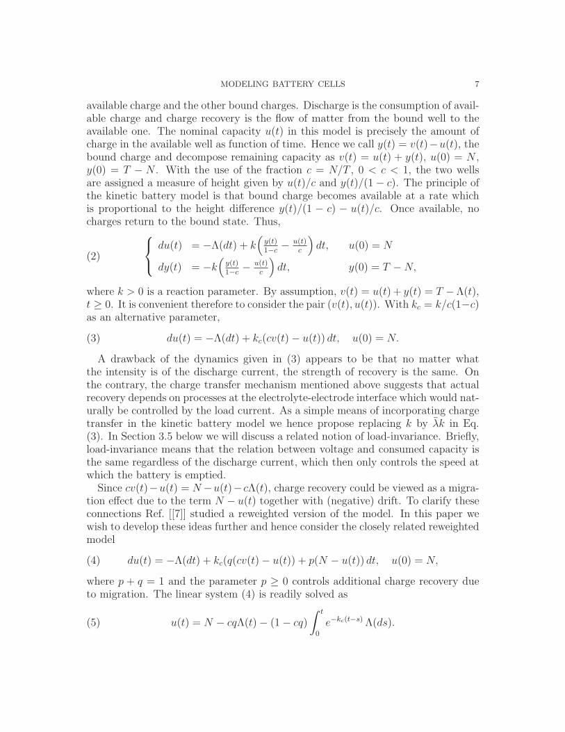
Here the relation to remaining capacity is λt = u(t, 0)− v(t) +Nℓ, and hence

u = (v − u)ωρ

ℓ+N(1− ωρ)−

λ

κℓ

∞∑

n=1

n2π2(1− e−2κ(ρ2+n2π2)(u−v+Nℓ)/λ)

(ρ2 + n2π2)2,


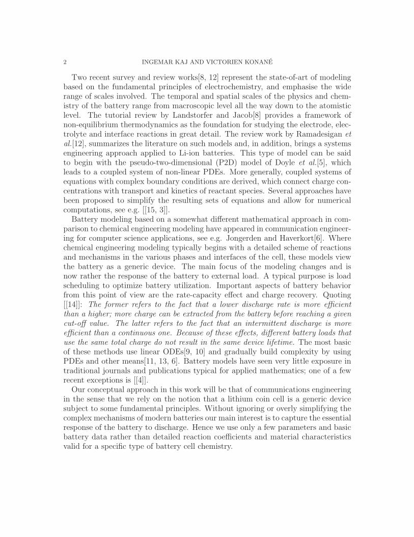
which is an autonomous system for (v, u) = (v(t), u(t, 0)). Figure 1 indicates thetypical shape of solution curves (v, u) for a few arbitrary parameter values, in par-ticular ℓ = (T −N)/N = 9.

0 100 200 300 400 500 600 700 800 900 10000

20

40

60

80

100

Figure 1. T = 1000, N = 100, λ = 1000, κ = 0.5, µ = 0, ρ = 0, 0.1,0.2, 0.5;

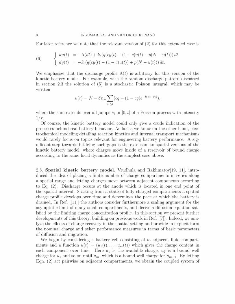
In greater generality, by replacing λt in (14) with u(t, 0)− v(t) +Nℓ,

u(t, 0) =ρN

ρ− µ+

2ρN

1− e−2δ+

2δ

1− e−2δ

1

ℓ(v(t)− u(t, 0))

+4µN∞∑

n=1

((−1)neδ − 1)n2π2

(δ2 + n2π2)2e−2κ(δ2+n2π2)(u(t,0)−v(t)+Nℓ)/λ

− λ

κℓ

∞∑

n=1

n2π2

(δ2 + n2π2)2(1− e−2κ(δ2+n2π2)(u(t,0)−v(t)+Nℓ)/λ),

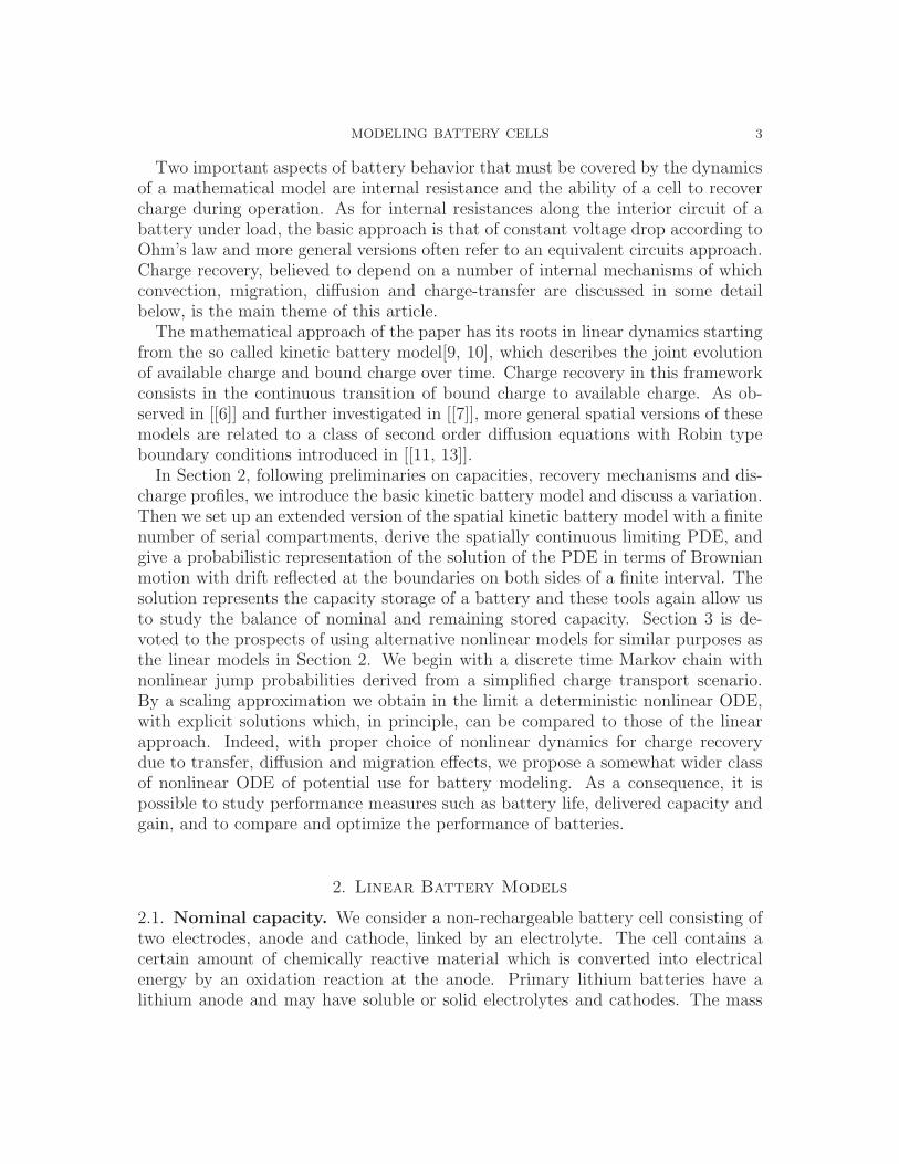
which is again an autonomous systems for nominal versus remaining capacity. Asan illustration Figure 2 shows solution traces (v, u) for fixed values of T . N , λ andκ, and with four different combinations of µ and ρ which all give approximately thesame utilization of the total available battery capacity.

0 100 200 300 400 500 600 700 800 900 10000

20

40

60

80

100

Figure 2. T = 1000, N = 100, λ = 1000, κ = 0.5, various combina-tions of µ and ρ


3. Nonlinear Battery Models

In this section we will introduce an approach to nonlinear battery modeling whichbegins with a discrete time Markov chain model moving on a set of bivariate statesrepresenting nominal and remaining capacities. The chain has nonlinear jump prob-abilities which we arrive at by analyzing a simplified transport system of chargesunder diffusion and migration. As a next step we investigate the scaled capacitiesas the number of slots per time unit tends to infinity and the discharge processconverges to that of a constant rate. In the limit we obtain deterministic capacityfuntions identified as the solution of a nonlinear ordinary differential equation. In-formed by these findings we then consider a class of nonlinear ODEs which can besolved explicitly. The solutions arising in this manner potentially reflect the non-linear dynamics of capacity under discharge of the battery. In addition we indicatetwo further directions of probabilistic modeling. One is to study the deviation ofthe Markov chain from its deterministic limit and describe the scaled fluctuationsin terms of a diffusion process. Finally we consider the deterministic limit processmodified to operate under random discharge, and compare this situation with theprevious cases.

3.1. Markov chain model in slotted time. We consider a discrete time Markovchain (Vn, Xn)n≥0 defined on the state space E = [0, T ]× [0, N ], modeling

Vn = remaining capacity [Ah] in time slot n

Xn = nominal capacity [Ah] in time slot n.

We assume that N and T are integer multiples of δ and that all jumps are of size δ.All jumps in the first coordinate are downwards. Jumps in the second are allowedto be both up and down as long as Xn ≤ N . The battery is discharged randomlyat constant current δ with probability q per slot. Letting

Zn = number of load units discharged in slot n, n ≥ 1.

where {Zi} is a sequence of i.i.d random variables with P (Zi = 1) = 1 − P (Zi =0) = q, it follows that Λn = δ

∑ni=1 Zi is the accumulated discharge at slot n and

Vn = T − Λn the remaining charge in the battery after n slots. The expecteddischarge rate is λ = E(Λn)/n = δq. Given the sequence (Vn)n≥0 as input we model(Xn)n≥0 as a Markov chain modulated by (Vn). All jumps down of (Xn) are inheritedfrom the discharge profile and follow those of (Vn). Jumps up will occur according toa Markovian dynamics chosen so as to reflect the recovery properties of the battery.In slot n + 1 the transition probabilities depend on the current state Xn and thecurrent discharge information stored in Vn.

Transport system. In an attempt to model charge recovery the battery cell is thoughtto consist of a randomly structured, electroactive material, which allows transportof charge carrying species through the electrolyte by liquid or solid state diffusion.


Internal charge recovery relies on access to transportation channels of enough con-nectivity to allow the material to pass from one node to the other. Also, thesechannels must be “activated” by a sufficient amount of previous discharge events.To try to describe such a system, we introduce

Kn = available concentration of charge in slot n

Ln = number of charge-carrying migration channels in slot n

Mn = number of channels in slot n activated by electrons at the cathode.

Conditional on (Vn, Xn), the updates Kn+1 and Ln+1 are assumed to have Poissondistributions, such that for given nonnegative parameters α > 0 and β > 0

Kn+1 ∈ Po(Vn, β), Ln+1 ∈ Po(α(N −Xn)),

and Mn+1 is binomially sampled from Ln+1, so that

Mn+1 ∈ Bin(Ln+1, q)d= Bin(N −Xn, qα)

d∼ Po(qα (N −Xn)).

In case there is no discharge in slot n, that is Zn = 0, then the battery cell is ableto recover one unit of charge if both Kn ≥ 1 and Mn ≥ 1. Hence

Vn+1 = Vn − δZn+1

Xn+1 = Xn − δZn+1 + δ(1− Zn+1)1{Kn+1≥1,Mn+1≥1}

The dynamics specified by this recursive relation is that, given (Vn, Xn) = (v, x), ifZn+1 = 1 then the transition in slot n+ 1 is (v, x) → (v − δ, x− δ) and if Zn+1 = 0then

(v, x) →{

(v, x+ δ) with probability (1− e−βv)(1− e−αq(N−x))(v, x) -”- 1− (1− e−βv)(1− e−αq(N−x)).

Together these relations define a bivariate Markov chain model (Vn, Xn)n≥0 withdynamics specified by

(v, x) →

(v − δ, x− δ) with prob. q(v, x+ δ) -”- (1− q)(1− e−βv)(1− e−αq(N−x))(v, x) -”- (1− q)(1− (1− e−βv)(1− e−αq(N−x)))

and, typically, initial condition (V0, X0) = (T,N). We obtain a drift function and avariance function for the Markov chain from

E(Xn+1 −Xn|(Vn, Xn)) = −qδ + (1− q)δ(1− e−βVn)(1− e−αq(N−Xn))

and

E((Xn+1 −Xn)2|(Vn, Xn)) = qδ2 + (1− q)δ2(1− e−βVn)(1− e−αq(N−Xn))


3.2. Continuous time approximation. The drift function m(v, x) = E(Xn+1 −Xn|Vn = v,Xn = x) suggests a relevant, approximating ODE for the Markov chain.To formalize this limit procedure it is convenient to introduce a scaling parameterm ≥ 1. At scaling level m the number of slots per unit time is m and the dischargecurrent jump size is δ/m rather than δ. Consider

Xmn = nominal capacity in slot n at scaling level m

and define for continuous time t ≥ 0,

X(m)(t) = Xm[mt].

Similarly, let Λmn be the scaled discharge process with δ replaced by δ/m and put

Λ(m)(t) = Λm[mt], V (m)(t) = T − Λ(m)(t).

Then

Λ(m)(t) =δ

m

[mt]∑

k=1

Zi =qδ[mt]

m+

√q(1− q)δ2

m

1√m

[mt]∑

k=1

Zi − q√q(1− q)

.

By the functional central limit theorem we may introduce a Wiener process W1(t)and for large m wiew V (m)(t) as an approximation of the continuous time remainingcapacity function Vt = T − λt, in the sense

dV (m)(t) = −λ dt+σ√m

dW1(t), V (m)(0) = T,

where σ2 = q(1−q)δ2 and the approximation error is of the order 1/√m. Moroever,

by considering the differential change of X(m)(t) over a time interval (t, t+h) whereh = 1/m,

E(X(m)(t+ h)−X(m)(t)|(V (m)(t), X(m)(t)) = (v, x))

= h(− λ+ (1− q)δ(1− e−βv)(1− e−αq(N−x))

)

and

E((X(m)(t+ h)−X(m)(t))2|(V (m)(t), X(m)(t)) = (v, x))

= h1

m

(λδ + (1− q)δ2(1− e−βv) (1− e−αq(N−x))

).

As above we obtain a deterministic limit equation for large m by applying a diffusionapproximation with the diffusion term of magnitude 1/

√m. To simplify notation

we put

f(v, x) = δ(1− q)(1− e−βv) (1− e−αq(1−x)).

Then

dX(m)(t) = −λ dt+ f(V (m)(t), X(m)(t)) dt+

√λδ

m+

δ

mf(V (m)(t), X(m)(t)) dW2(t)


Here, W2 is another Wiener process. Since V (m) and X(m) have simultaneous jumps,W1 and W2 are dependent with a non-zero covariance.

3.3. Deterministic approximation of the Markov chain model. As m → ∞,the stochastic differential equations for V (m) and X(m) simplify and become theordinary differential equation

(15)x′t = −δq + (1− q)δ(1− e−βvt)(1− e−αq(N−xt)), x0 = N,

v′t = −δq, v0 = T.

Recalling λ = δq, the solution is vt = T − λt and

xt = N − 1

αqln(1− αq

∫ t

0

h(s)

h(t)λds

),

where

h(t)/h(0) = exp{λαt− (1− q)αe−βT (eλβt − 1)/β

}.

Hence

αq

∫ t

0

h(s)

h(t)λds = αq

∫ λt

0

exp{− αs+ (1− q)αeλβt−βT (1− e−βs)/β

}ds

and so

(16) xt = N − 1

αqln(1− αq

∫ T−vt

0

exp{− αs+ (1− q)αe−βvt(1− e−βs)/β

}ds).

Thus, in analogy with the results obtained for the kinetic battery models in theprevious section, it follows that (v, x) = (v(t), x(t)) is an autonomous system fromwhich we can read off the nominal capacity, and hence the voltage, as a function ofremaining capacity.

On-off discharge pattern. In the Markov chain model of section 3.1, we consideredrandom discharge at current δ with probability q per slot, which converged by thelaw of large numbers to a constant discharge pattern Λ(t) = λt, λ = δq, under theapproximation scheme of section 3.3. An alternative would be to run the Markovchain (Vn, Xn) relative to a given discharge sequence (Zn), such that in the scalinglimit emerges an on-off discharge pattern as discussed in section 2.3. We recallthat (Jt) is the piecewise constant indicator function which is one during periods

when the battery is under load and zero otherwise and that Vt = T − δ∫ t

0Ju du is

the remaining capacity at time t. As the degree of resolution increases by takingm → ∞ we then expect the process of nominal capacity, (X(m))t≥0, to convergeto a deterministic limiting function (Xt)t≥0, which solves the ordinary differentialequation

dXt = −δJt dt+ δ(1− Jt)(1− eαq(N−Xt))(1− e−βVt) dt.


Then

eαq(N−Xt) dXt = δ(eαq(N−Xt) − 1){−Jt + (1− Jt)(1− e−βVt)} dt− δJt dt

and so, by introducing a generating factor Ht defined by

d

dtlnHt = αqδ(−Jt + (1− Jt)(1− e−βVt)),

hence

Ht = H0 exp{αqδ

∫ t

0

(−Ju + (1− Ju)(1− e−βVu)) du},

we can solve for Xt and obtain

Xt = N − 1

αqln(1 +

αqδ

Ht

∫ t

0

JsHs ds)

With λ = qδ this may be written

Xt = N − 1

αqln(1 + λα

∫ t

0

Js eλα

∫ t

s(Ju−(1−Ju)(1−e−βVu )) du ds

),

which is a closed form solution for capacity in terms of the given discharge pro-file, coded by (Jt) and (Vt) with parameters δ and q, and the additional batteryparameters α and β.

3.4. Deviation from deterministic behavior. We have found a deterministicfunction (vt, xt) which satisfies the ordinary differential equation (15), in the limitm → ∞ of the scaled Markov chain (V (m)(t), X(m)(t))t≥0 with constant dischargerate λ. Now we introduce the quantities

νm(t) =√m(V (m)(t)− vt), ξm(t) =

√m(X(m)(t)− xt),

and study the fluctuations of the scaled Markov chain around (vt, xt). With W1 andW2 as in section 3.2 we obtain for large m,

dνm(t) = σ dW1(t)

dξm(t) =√m(f(V (m)(t), X(m)(t))− f(vt, xt)) dt

+√

λδ + δf(V (m)(t), X(m)(t)) dW2(t),

where ν(0) = ξ(0) = 0. It follows by a Taylor expansion of f(v, x) that

dξm(t) = f ′v(vt, xt)νm(t) dt+ f ′

x(vt, xt)ξm(t) dt

+√λδ + δf(V (m)(t), X(m)(t)) dW2(t).

In the scaling limit m → ∞ we therefore expect that the fluctuation process ξm(t)converges to a diffusion process ξ(t), such that

dξ(t) = f ′v(vt, xt)σW1(t) dt+ f ′

x(vt, xt)ξ(t) dt+√λδ + δf(vt, xt) dW2(t).


This stochastic differential equation for ξ(t) can be seen as a generalized OrnsteinUhlenbeck process

dξ(t) = atW1(t) dt+ bt ξ(t) dt+ ct dW2(t),

with time-inhomogeneous drift and variance coeffecients bt and ct, which is alsomodulated by an additional, random, drift atW1(t).

3.5. A general class of nonlinear ODE battery capacity models. To derivethe capacity dynamics in (16) we were guided by a Markov chain argument basedon a simplified view of charge transport inside the battery cell. In this final sectionwe mention a more general class of deterministic non-linear recovery models for thedynamics of nominal capacity and state of charge. Again we write xt for nominalcapacity and vt for the remaining capacity in the cell as functions of time t ≥ 0.The general principle for charge recovery is that of balancing the discharge rate

in xt by a positive drift of the nominal capacity due to the release and transportof stored charges. It is reasonable that such effects are proportional to the appliedaverage load λ and exist as long as the theoretical capacity of the cell has not yetbeen fully consumed, that is vt ≥ 0. Furthermore, the gain in capacity due torecovery depends on the migration of charge-carriers, and the strength of this effectshould increase with the gap N−xt between maximal and actual capacity. Hence, tocapture charge recovery in the framework of one-dimensional differential equations,we may let F : [0,∞) → [0, 1] and G : [0,∞) → [0, 1] be non-decreasing functionswith F (0) = 0, G(0) = 0, and consider equations of the generic shape

(17) dxt = −Λ(dt) + λF (N − xt)G(vt) dt, t ≤ t0, x0 = N,

where t0 is battery life defined as the maximal time t for which xt ≥ 0. For now,however, we keep the setting of (16) and put F (u) = 1− e−au, where a is a positiveconstant which should measure the strength of migration of charges due to theexisting electric field in the battery.

Constant discharge recovery mechanism. Suppose the battery is discharged contin-uously at constant current λ > 0 with discharge profile Λ(t) = λt. We consider thespecial case of (17) given by the ODE

(18) x′t = −λ+ λ(1− e−a(N−xt))G(vt), X0 = N.

Because of the separation of variables we may write

ht(ea(N−xt) − 1) = λa

∫ t

0

hs ds

where

ln(ht/h0) = −λa

∫ t

0

(1−G(vs)) ds,


and hence

xt = N − 1

aln(1 + λa

∫ t

0

eλa∫ t

s(1−G(vu)) du ds

).

Equivalently,

xt = N − 1

aln(1 + a

∫ T−vt

0

exp{a

∫ vt+s

vt

(1−G(u)) du}ds).

It is immediate in this model that the pair (vt, xt) is autonomous so that nominalcapacity x = x(v) can be viewed as a function of remaining capacity only. Moreover,the capacity dynamnics is load-invariant in the sense that the curve (v, x(v)) doesnot depend on λ. In other words, batteries drained using different choices of λ willexhibit different battery lifes, longer the smaller intensity of the current, but theused capacity T − v at end of life will be the same in each case.

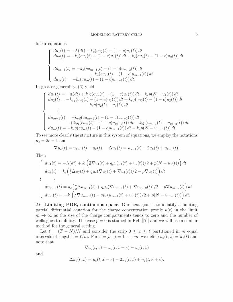
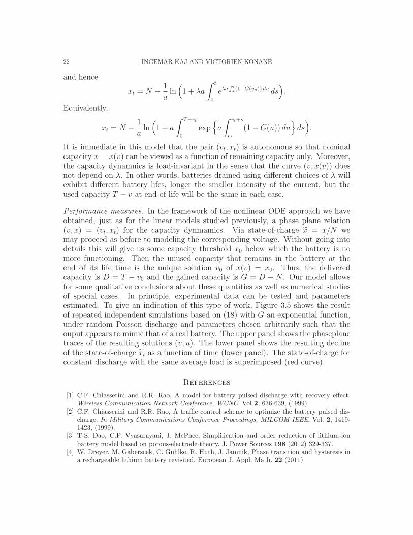
Performance measures. In the framework of the nonlinear ODE approach we haveobtained, just as for the linear models studied previously, a phase plane relation(v, x) = (vt, xt) for the capacity dynmamics. Via state-of-charge x = x/N wemay proceed as before to modeling the corresponding voltage. Without going intodetails this will give us some capacity threshold x0 below which the battery is nomore functioning. Then the unused capacity that remains in the battery at theend of its life time is the unique solution v0 of x(v) = x0. Thus, the deliveredcapacity is D = T − v0 and the gained capacity is G = D − N . Our model allowsfor some qualitative conclusions about these quantities as well as numerical studiesof special cases. In principle, experimental data can be tested and parametersestimated. To give an indication of this type of work, Figure 3.5 shows the resultof repeated independent simulations based on (18) with G an exponential function,under random Poisson discharge and parameters chosen arbitrarily such that theouput appears to mimic that of a real battery. The upper panel shows the phaseplanetraces of the resulting solutions (v, u). The lower panel shows the resulting declineof the state-of-charge xt as a function of time (lower panel). The state-of-charge forconstant discharge with the same average load is superimposed (red curve).

References

[1] C.F. Chiasserini and R.R. Rao, A model for battery pulsed discharge with recovery effect.Wireless Communication Network Conference, WCNC, Vol 2, 636-639, (1999).

[2] C.F. Chiasserini and R.R. Rao, A traffic control scheme to optimize the battery pulsed dis-charge. In Military Communications Conference Proceedings, MILCOM IEEE, Vol. 2, 1419-1423, (1999).

[3] T-S. Dao, C.P. Vyasarayani, J. McPhee, Simplification and order reduction of lithium-ionbattery model based on porous-electrode theory. J. Power Sources 198 (2012) 329-337.

[4] W. Dreyer, M. Gaberscek, C. Guhlke, R. Huth, J. Jamnik, Phase transition and hysteresis ina rechargeable lithium battery revisited. European J. Appl. Math. 22 (2011)


0 1000 2000 3000 4000 5000 6000 7000 8000 9000 100000

100

200

300

400

500

Remaining theoretical capacity

Nom

inal

cap

acity

0 0.5 1 1.5 2 2.5 3 3.5 4

x 104

0

0.2

0.4

0.6

0.8

1

time

stat

e−of

−ch

arge

[5] M. Doyle, T.F. Fuller, J. Newman, Modeling of galvanostatic charge and discharge of thelithium/polymer/insertion cell. J. Electrochem. Soc. 140 (1993) 1526-1533.

[6] M. R. Jongerden and B.R.H.M Haverkort, which battery model to use? In:IEEE/IET Soft-ware, Vol 3 Issue 6, 445 - 457, (2009).

[7] I. Kaj and V. Konane, Analytical and stochastic modelling of battery cell dynamics. Proceed.19th Intern. Conf. Analytic and Stochastic Modelling Techn. and Appl. K. Al-Begain, D.Fiems, and J.-M. Vincent (Eds.): ASMTA 2012, Lecture Notes in Computer Science, Vol7314, 240–254, 2012.

[8] M. Landstorfer, T. Jacob, Mathematical modeling of intercallation batteries at the cell leveland beyond. Chem. Soc. Rev. (2013) 42, 3234-3252.

[9] J. Manwell and J. McGowen, Lead acid battery storage model for hybrid energy systems.Solar Energy 50, 399-405, (1993).

[10] J. Manwell, J. McGowen: Extension of the kinetic battery model for wind/hybrid powersystems. Proc. fifth European Wind Energy Association Conf. 1994, 284-289.

[11] D. Rakhmatov, S. Vrudhula, Energy Management for Battery-Powered Embedded Systems.ACM Transactions on Embedded Computing Systems, 2:3, (2003), 277-324.

[12] V. Ramadesigan, P.W.C Northrop, S. De, S. Sananthagopalan, R.D. Braatz and V.R. Sub-ramanian, Modeling and simulation of Lithium-ion batteries from a systems engineering per-spective. j. Electrochem. Soc. 159:3 (2012), R31-R45.

[13] R. Rao, S. Vrudhula, D. Rakhmatov, Battery modeling for energy-aware system design. IEEEComputer 3612 (2003) 77-87.

[14] C. Rohner, L.M. Feeney, and P. Gunningberg, Evaluating battery models in wireless sen-sor networks. 11th International Conference on Wired/Wireless Internet Communication(WWIC), Lecture Notes in Computer Science Vol 7889, 2013.

[15] V. Subramaniam, V. Boovaragavan, V. Ramadesigan, M. Arabandi, Mathematical model re-formulation for Lithium-ion battery simulations: galvanostatic boundary conditions. J. Elec-trochem. Soc. 156(4) A260-A271 (2009).

[16] Svensson, L.E.O., The term structure of interest rate differentials in a target zone, Theory andSwedish data. Seminar Paper 466, Institute for International Economic Studies, StockholmUniversity 1990.


[17] S. Vrudhula, D. Rakhmatov and D.A. Wallach A model for battery lifetime analysis fororganizing applications on a pocket computer, IEEE Trans. VLSI Syst., (2003), 11,(6), 1019-1030.

[18] Veestraeten, D.: The conditional probability density function for a reflected Brownian motion.Computational Economics 24, 185-207 (2004)

[19] S. Vrudhula and D. Rakhmatov, An analytical high-level battery model for use in energy man-agement of portable electronic systems, Proc. Int. Conf. Computer Aided Design (ICCAD’01),(2001), 488-493.

[20] S. Vrudhula, D. Rakhmatov and D.A. Wallach, Battery lifetime predictions for energyawarecomputing, Proc. 2002 Int. Symp. Low Power Electronics and Design(ISLPED’02), (2002),154-159.

Department of Mathematics, Uppsala University, P.O. Box 480, SE 751 06 Upp-

sala, Sweden, [email protected]

International Science Program, Uppsala University, Department of Mathemat-

ics, University of Ouagadougou, Burkina Faso, [email protected]

MODELING VOLTAGE IN BATTERY CELLS - Uppsala …ikaj/preprints/modvoltagebasic2.pdf · MODELING...

Documents

Transcript of MODELING VOLTAGE IN BATTERY CELLS - Uppsala …ikaj/preprints/modvoltagebasic2.pdf · MODELING...