MODELING TSUNAMI INUNDATION FROM A … tsunami inundation from a cascadia subduction zone earthquake...

UNITED STATESDEPARTMENT OF COMMERCE

Carlos M. GutierrezSecretary

NATIONAL OCEANIC ANDATMOSPHERIC ADMINISTRATION

VADM Conrad C. Lautenbacher, Jr.Under Secretary for Oceansand Atmosphere/Administrator

Office of Oceanic and Atmospheric Research

Richard W. SpinradAssistant Administrator

NOAA Technical Memorandum OAR PMEL-137

MODELING TSUNAMI INUNDATION FROM A CASCADIASUBDUCTION ZONE EARTHQUAKE FOR LONG BEACHAND OCEAN SHORES, WASHINGTON

Angie J. Venturato1,2

Diego Arcas1,2

2Joint Institute for the Study of the Atmosphere and Ocean (JISAO)University of Washington, Seattle, WA

1NOAA/Pacific Marine Environmental LaboratorySeattle, WA

Pacific Marine Environmental LaboratorySeattle, WAJuly 2007

Utku Kânoğlu3

3Department of Engineering Sciences, Middle East Technical University,Ankara, TURKEY

NOTICE from NOAA

Mention of a commercial company or product does not constitute an endorsement byNOAA/OAR. Use of information from this publication concerning proprietary productsor the tests of such products for publicity or advertising purposes is not authorized. Anyopinions, findings, and conclusions or recommendations expressed in this material are thoseof the authors and do not necessarily reflect the views of the National Oceanic and Atmo-spheric Administration.

Contribution No. 2949 from NOAA/Pacific Marine Environmental Laboratory

Also available from the National Technical Information Service (NTIS)(http://www.ntis.gov)

ii

Contents

List of Figures iii

Abstract 1

1 Background 1

2 Study Area 22.1 Coastal Morphology . . . . . . . . . . . . . . . . . . . . . . . 2

3 Tsunami Source 5

4 Tsunami Model 64.1 Digital Elevation Model Development . . . . . . . . . . . . . 84.2 Model Setup . . . . . . . . . . . . . . . . . . . . . . . . . . . 8

5 Model Results 85.1 Offshore Dynamics . . . . . . . . . . . . . . . . . . . . . . . . 85.2 Inundation Details . . . . . . . . . . . . . . . . . . . . . . . . 10

5.2.1 Ocean Shores . . . . . . . . . . . . . . . . . . . . . . . 125.2.2 Long Beach Peninsula . . . . . . . . . . . . . . . . . . 13

6 Discussion 166.1 Potential Sources of Error . . . . . . . . . . . . . . . . . . . . 16

6.1.1 Limitations of the tsunami source . . . . . . . . . . . 166.1.2 Limitations of the DEM . . . . . . . . . . . . . . . . . 17

6.2 Model Comparison . . . . . . . . . . . . . . . . . . . . . . . . 19

7 Conclusions and Recommendations for Future Work 21

8 References 23

Appendix A: Data Credit 25

Appendix B: Modeling Products 26

List of Figures

1 (a) Extent and resolution of each digital elevation model (DEM)used in the study. (b) The Columbia River littoral cell . . . . . . 3

2 Study area for tsunami inundation . . . . . . . . . . . . . . . . . 43 Initial deformation . . . . . . . . . . . . . . . . . . . . . . . . . . 64 Extent of model grids for Ocean Shores (left panel) and Long

Beach (right panel) . . . . . . . . . . . . . . . . . . . . . . . . . . 75 Snapshots of modeled tsunami propagation . . . . . . . . . . . . 10

iii

iv Contents

6 Time series of wave heights and current speeds at select sites ofthe study region . . . . . . . . . . . . . . . . . . . . . . . . . . . 11

7 Modeled tsunami inundation at Ocean Shores . . . . . . . . . . . 128 Maximum inundation (left panel) and current speeds (right panel)

for the Ocean Shores region . . . . . . . . . . . . . . . . . . . . . 139 Modeled tsunami inundation of the Long Beach peninsula . . . . 1410 Maximum inundation (left panel) and current speeds (right panel)

for the Long Beach peninsula . . . . . . . . . . . . . . . . . . . . 1511 Proposed grid extent to reduce potential errors in the model setup 1712 Coverage area of the primary data sources used in the high-

resolution DEM. . . . . . . . . . . . . . . . . . . . . . . . . . . . 1813 Comparison of MOST and ADCIRC model simulations for Gold

Beach, Oregon . . . . . . . . . . . . . . . . . . . . . . . . . . . . 20

Modeling tsunami inundation from a Cascadia subduction zoneearthquake for Long Beach and Ocean Shores, Washington

A.J. Venturato1,2, D. Arcas1,2, and U. Kanoglu3

Abstract. The NOAA Center for Tsunami Research modeled tsunami inundation from a greatCascadia Subduction Zone earthquake for the coastal communities of Long Beach and Ocean Shores,Washington. A high-resolution numerical model was used to estimate tsunami propagation andinundation along the outer coast of southwest Washington. This effort was funded by the NationalTsunami Hazard Mitigation Program via a grant from the Emergency Management Division of theWashington State Military Department.

1. Background

A great (moment magnitude, Mw = 8.0 or higher) Cascadia Subduction Zone(CSZ) earthquake represents the most devastating tsunami threat in the Pa-cific Basin to Washington State (National Science and Technology Council,2005). Evidence from radiocarbon dating, Japanese historical records, andregional tribal accounts suggests that a great earthquake occurred along theCSZ in 1700 (Atwater et al. 1995; Satake et al., 1996; Yamaguchi et al.,1997). Petersen et al. (2002) estimate that another great CSZ earthquakehas a 10–14 percent chance of occurring within the next 50 years.

As a result of this threat, Washington developed tsunami hazard andevacuation maps for several at-risk communities along the Pacific coast.Long Beach and Ocean Shores were mapped in 2000 as a result of finiteelement modeling studies from the Oregon Graduate Institute of Scienceand Technology (OGI). Since 2000, both peninsulas have been surveyed us-ing high-resolution Light Detection and Ranging (LIDAR) systems to moreaccurately depict the topography. Additionally, improved grid developmenttechniques (Venturato, 2005) are available to reduce horizontal and verticalcontrol errors.

The Washington State Emergency Management Division provided a grantto the NOAA Center for Tsunami Research (NCTR) to reanalyze potentialtsunami inundation at Long Beach and Ocean Shores due to a great CSZearthquake. This effort includes:

• Using improved techniques to develop a new digital elevation modelbased on LIDAR and other updated elevation data.

• Using the finite difference Method of Splitting Tsunami (MOST) modelinstead of the original OGI finite element model known as ADCIRC.

1NOAA, Pacific Marine Environmental Laboratory, Seattle, WA, USA2Joint Institute for the Study of the Ocean and Atmosphere (JISAO), Box 354235,

University of Washington, Seattle, WA 98115-4235, USA3Department of Engineering Sciences, Middle East Technical University, 06531 Ankara,

TURKEY

2 Venturato et al.

• Using a Mw 9.1 CSZ earthquake with Washington asperity to matchthe “worst-case” tsunami source scenario developed in 2000.

The methodology and results of this effort are presented in the followingsections. The results are compared to prior work and suggestions for furtherresearch are included.

2. Study Area

The study area lies along the southwest Washington coast within the Colum-bia River littoral cell (Fig. 1). The study region includes Ocean Shores,Ocean City, Oyhut, and Sampson in Grays Harbor County; and the commu-nities of Long Beach, Klipsan Beach, Ilwaco, Seaview, Ocean Park, Surfside,Oysterville, and Nahcotta on the Long Beach peninsula in Pacific County(Fig. 2). Six State Parks, a National Wildlife Refuge, and several recre-ational areas also reside within the area.

The city of Ocean Shores covers most of the barrier beach that sits be-tween the Pacific Ocean and Grays Harbor. Oyhut, Sampson, and OceanCity are small communities north of Ocean Shores. Ocean Shores has apopulation of 3,270 based on the 2000 U.S. Census (Grays Harbor County,2005).

Tourism is the primary economic engine for the region with over threemillion visitors annually (Ocean Shores Chamber of Commerce, 2005). Thepeninsula has a 9.5-km beach on its western shore and a marina, passengerferry, and municipal airport along its eastern shore. The Oyhut WildlifeRecreation Area consists of a saltwater marsh and resides on the southeastcorner of the peninsula.

The Long Beach Peninsula serves as a barrier between the Pacific Oceanand the Willapa Bay estuary. It has the longest (45 km) natural beach in theUnited States. The region’s economy consists primarily of tourism, shellfishharvesting, recreational fishing, and logging. The Port of Peninsula sitswithin Willapa Bay, and the Port of Ilwaco lies within the Columbia River.Long Beach and Ilwaco are the largest communities on the peninsula, withpopulations of 1,340 and 945, respectively (Pacific County, 2003).

2.1 Coastal Morphology

The Columbia River littoral cell is a highly dynamic region that experiencesalternating patterns of progradation and erosion due to longshore sedimenttransport, tidal forcing, and intense winter storms (Peterson et al., 1999).Additionally, geologic evidence has shown that past great Cascadia earth-quakes have caused catastrophic beach retreat due to coseismic subsidence(Atwater, 1987; Doyle, 1996). The natural episodic pattern of prograda-tion and retreat have been altered in recent times (1870 to present) due toanthropogenic development.

Modeling Long Beach and Ocean Shores, WA, tsunami inundation 3

Fig

ure

1:(a

)E

xten

tan

dre

solu

tion

ofea

chdi

gita

lel

evat

ion

mod

el(D

EM

)us

edin

the

stud

y.T

helo

w-r

esol

utio

nD

EM

sco

nsis

tof

bath

ymet

ric

dept

hva

lues

only

.T

hehi

gh-r

esol

utio

nD

EM

cons

ists

ofba

thym

etry

and

topo

grap

hy.

The

tria

ngle

sde

pict

the

wat

er-lev

elst

atio

nsus

edto

conv

ert

vert

ical

valu

esto

Mea

nH

igh

Wat

er(M

ofje

ldet

al.,

2004

).(b

)T

heC

olum

bia

Riv

erlit

tora

lce

ll.T

heLon

gB

each

peni

nsul

asi

tsw

ithi

nth

eLon

gB

each

sub-

cell,

and

Oce

anSh

ores

lies

wit

hin

the

Nor

thB

each

sub-

cell.

4 Venturato et al.

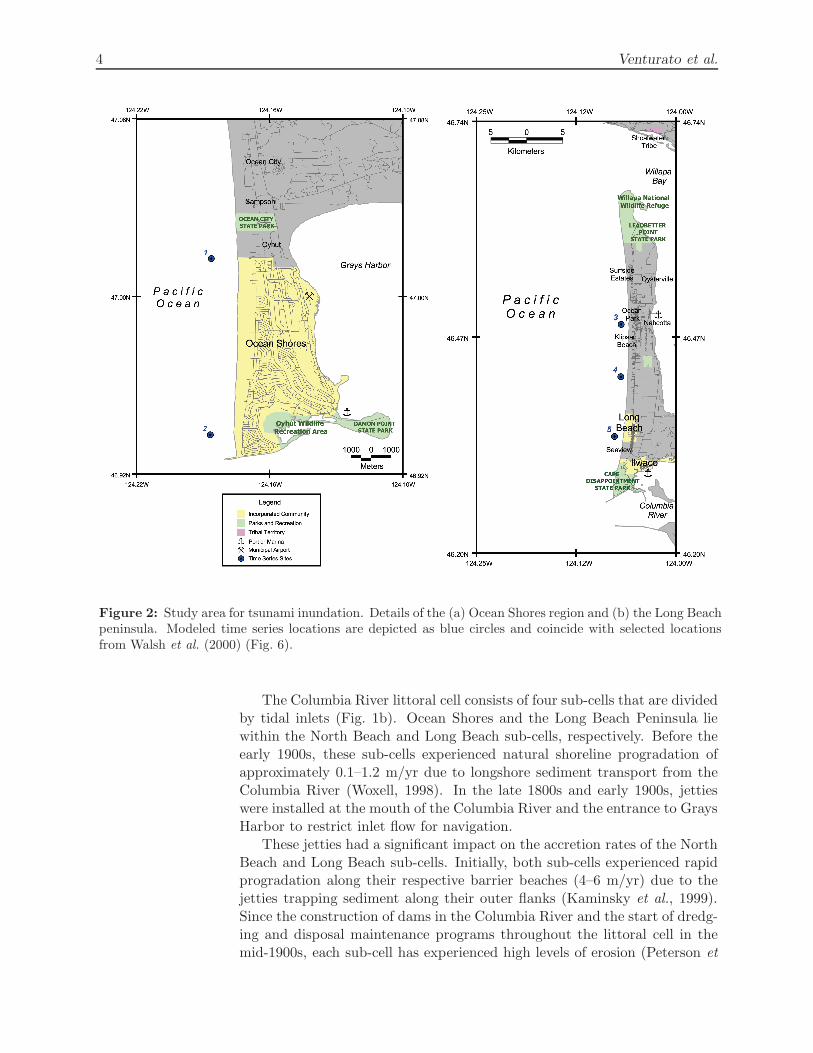
Figure 2: Study area for tsunami inundation. Details of the (a) Ocean Shores region and (b) the Long Beachpeninsula. Modeled time series locations are depicted as blue circles and coincide with selected locationsfrom Walsh et al. (2000) (Fig. 6).

The Columbia River littoral cell consists of four sub-cells that are dividedby tidal inlets (Fig. 1b). Ocean Shores and the Long Beach Peninsula liewithin the North Beach and Long Beach sub-cells, respectively. Before theearly 1900s, these sub-cells experienced natural shoreline progradation ofapproximately 0.1–1.2 m/yr due to longshore sediment transport from theColumbia River (Woxell, 1998). In the late 1800s and early 1900s, jettieswere installed at the mouth of the Columbia River and the entrance to GraysHarbor to restrict inlet flow for navigation.

These jetties had a significant impact on the accretion rates of the NorthBeach and Long Beach sub-cells. Initially, both sub-cells experienced rapidprogradation along their respective barrier beaches (4–6 m/yr) due to thejetties trapping sediment along their outer flanks (Kaminsky et al., 1999).Since the construction of dams in the Columbia River and the start of dredg-ing and disposal maintenance programs throughout the littoral cell in themid-1900s, each sub-cell has experienced high levels of erosion (Peterson et


al., 1999). Additionally, the lack of sand has led to deepening waters off-shore, making these beaches more susceptible to rapid beach retreat duringintense storms and seismic events.

Both Ocean Shores and the Long Beach peninsula experience beach alter-ation due to these anthropogenic effects. Several erosion hotspots (Fig. 1b)are threatening state parks, natural habitat, and coastal development alongeach barrier beach (Washington State Department of Ecology, 2007).

3. Tsunami Source

Tsunami generation by a rupture along the CSZ is considered for this study.The earthquake would create onshore subsidence and large offshore upliftgenerating an intense tsunami with two fronts: one directed toward thePacific Northwest coast as evidenced by geologic evidence (Atwater et al.,1995), and the other directed offshore as evidenced by historic Japaneserecords (Satake et al., 1996).

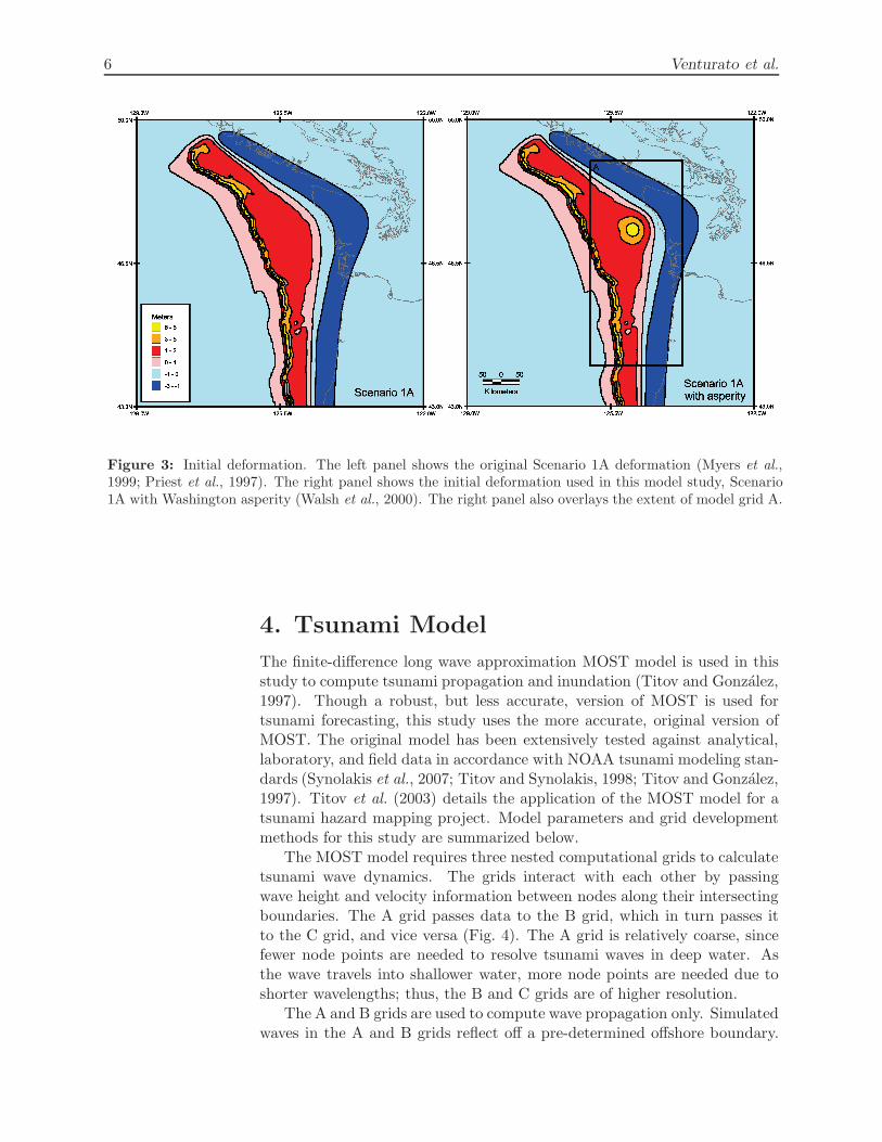
Priest et al. (1997) and Myers et al. (1999) developed six scenarios thatconsider various slip distributions along locked and transition zones along theCSZ to match paleoseismic evidence. Walsh et al. (2000) added additionalcoseismic slip, or an asperity, offshore of Washington to one of these scenar-ios (Scenario 1A) based on the presence of low-gravity anomalies detected bysatellite, bathymetry, and seismic profiling (Wells and Blakely, 2003). Sce-nario 1A plus the Washington asperity is considered the worst-case scenariofor tsunami inundation at Long Beach and Ocean Shores.

The 4.5-m asperity was generated using an elliptical Gaussian distribu-tion centered at 47.324◦N, 124.94◦W. The resulting slip distribution corre-sponds with a Mw 9.1 earthquake with a total uplift (asperity amplitude plusScenario 1A deformation) of 6 m in the high-slip area (Fig. 3). Additionalparameters are provided in Table 1.

Table 1: Tsunami source parameters (CSZ Scenario 1A plusWashington asperity). The slip distribution is displayed inFig. 3.

Parameter Value

Rupture length along fault 1050 kmRupture width 70 kmAverage slip along fault 17.5 mMoment magnitude 9.1Asperity location 47.324◦N, 124.94◦WAsperity amplitude 4.5 mElliptical axis orientation 0◦

Elliptical semi-major axis 38.45 kmElliptical semi-minor axis 25.63 km

6 Venturato et al.

Figure 3: Initial deformation. The left panel shows the original Scenario 1A deformation (Myers et al.,1999; Priest et al., 1997). The right panel shows the initial deformation used in this model study, Scenario1A with Washington asperity (Walsh et al., 2000). The right panel also overlays the extent of model grid A.

4. Tsunami Model

The finite-difference long wave approximation MOST model is used in thisstudy to compute tsunami propagation and inundation (Titov and Gonzalez,1997). Though a robust, but less accurate, version of MOST is used fortsunami forecasting, this study uses the more accurate, original version ofMOST. The original model has been extensively tested against analytical,laboratory, and field data in accordance with NOAA tsunami modeling stan-dards (Synolakis et al., 2007; Titov and Synolakis, 1998; Titov and Gonzalez,1997). Titov et al. (2003) details the application of the MOST model for atsunami hazard mapping project. Model parameters and grid developmentmethods for this study are summarized below.

The MOST model requires three nested computational grids to calculatetsunami wave dynamics. The grids interact with each other by passingwave height and velocity information between nodes along their intersectingboundaries. The A grid passes data to the B grid, which in turn passes itto the C grid, and vice versa (Fig. 4). The A grid is relatively coarse, sincefewer node points are needed to resolve tsunami waves in deep water. Asthe wave travels into shallower water, more node points are needed due toshorter wavelengths; thus, the B and C grids are of higher resolution.

The A and B grids are used to compute wave propagation only. Simulatedwaves in the A and B grids reflect off a pre-determined offshore boundary.


Figure 4: Extent of model grids for Ocean Shores (left panel) and Long Beach (right panel). Tsunamiinundation is computed in the C grid and wave propagation is computed in all three grids. Each inset showsthe details of the reflection boundary within the B grid. The dashed line represents the reflection boundarydepth (Table 3) used for each simulation. The arrows represent wave propagation and reflection betweengrids.

The boundary is chosen to limit model instabilities that may occur due to theseafloor being bared during wave recession. The C grid is used to computewave propagation and inundation on land; thus, no reflection boundary isimplemented in this grid (Fig. 4). In order to compute tsunami inundationaccurately, high-resolution bathymetry and topography are required in theC grid.

8 Venturato et al.

4.1 Digital Elevation Model Development

Three digital elevation models (DEMs) were developed for this study (Fig. 1a).Bathymetric, topographic, and shoreline data were collected from variousagencies and converted to standard units based on model specifications (Ta-ble 2). Because the MOST model does not include tidal dynamics, MeanHigh Water was used as the baseline vertical datum to simulate the in-undation scenario at high tide. This is a relatively conservative value forthe background water level, since the most probable level for the maximumheights of large tsunamis along the Pacific coast are closer to Mean SeaLevel (Mofjeld et al., 2007). Vertical datum transformations were appliedusing linearly interpolated values from official National Ocean Service (NOS)datums at water-level stations (Fig. 1a) along the Pacific Northwest coast(Mofjeld et al., 2004).

Data were analyzed and combined using methods described in Venturato(2005). Data sources used to develop the DEMs are provided in Appendix A.As in other tsunami inundation studies, the vegetation and manmade struc-tures were removed from the topography to produce a “bald-earth” DEM.

The DEMs were created using a simple method of Delauney triangulationand nearest neighbor interpolation. A spatial analysis was performed toensure quality from original data sources and consistency between DEMs.The 1/3-, 6-, and 36-arc-second DEMs were converted to ASCII raster gridsfor use in the tsunami model.

4.2 Model Setup

The DEMs were clipped and resampled to reduce the number of computa-tions required in the MOST model (Fig. 4, Table 3). A smoothing algorithmwas also applied to the computational grids to maintain model stability byreducing potential discontinuities due to single-node cells (i.e., offshore is-lands). The model grids are then adjusted for coseismic displacement byadding the deformation field (Fig. 3) to the vertical values in the grid.

As described previously, the gridded land surface does not contain veg-etation or man-made structures. In reality, these obstacles may alter theamount and pattern of tsunami inundation. Thus, the model includes aconservative friction coefficient to add roughness to the land surface (Man-ning parameter, n = 0.025). Though this value may be conservative, itrepresents a reasonable estimate given the lack of proven scientific studiesregarding tsunami forces on structures.

5. Model Results

5.1 Offshore Dynamics

The CSZ source creates 1–2 m of subsidence onshore with significant upliftoffshore (Fig. 3). This generates a leading depression wave along the entire


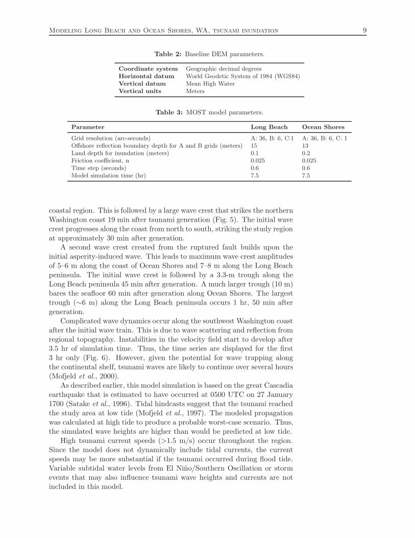
Table 2: Baseline DEM parameters.

Coordinate system Geographic decimal degreesHorizontal datum World Geodetic System of 1984 (WGS84)Vertical datum Mean High WaterVertical units Meters

Table 3: MOST model parameters.

Parameter Long Beach Ocean Shores

Grid resolution (arc-seconds) A: 36, B: 6, C:1 A: 36, B: 6, C: 1Offshore reflection boundary depth for A and B grids (meters) 15 13Land depth for inundation (meters) 0.1 0.2Friction coefficient, n 0.025 0.025Time step (seconds) 0.6 0.6Model simulation time (hr) 7.5 7.5

coastal region. This is followed by a large wave crest that strikes the northernWashington coast 19 min after tsunami generation (Fig. 5). The initial wavecrest progresses along the coast from north to south, striking the study regionat approximately 30 min after generation.

A second wave crest created from the ruptured fault builds upon theinitial asperity-induced wave. This leads to maximum wave crest amplitudesof 5–6 m along the coast of Ocean Shores and 7–8 m along the Long Beachpeninsula. The initial wave crest is followed by a 3.3-m trough along theLong Beach peninsula 45 min after generation. A much larger trough (10 m)bares the seafloor 60 min after generation along Ocean Shores. The largesttrough (∼6 m) along the Long Beach peninsula occurs 1 hr, 50 min aftergeneration.

Complicated wave dynamics occur along the southwest Washington coastafter the initial wave train. This is due to wave scattering and reflection fromregional topography. Instabilities in the velocity field start to develop after3.5 hr of simulation time. Thus, the time series are displayed for the first3 hr only (Fig. 6). However, given the potential for wave trapping alongthe continental shelf, tsunami waves are likely to continue over several hours(Mofjeld et al., 2000).

As described earlier, this model simulation is based on the great Cascadiaearthquake that is estimated to have occurred at 0500 UTC on 27 January1700 (Satake et al., 1996). Tidal hindcasts suggest that the tsunami reachedthe study area at low tide (Mofjeld et al., 1997). The modeled propagationwas calculated at high tide to produce a probable worst-case scenario. Thus,the simulated wave heights are higher than would be predicted at low tide.

High tsunami current speeds (>1.5 m/s) occur throughout the region.Since the model does not dynamically include tidal currents, the currentspeeds may be more substantial if the tsunami occurred during flood tide.Variable subtidal water levels from El Nino/Southern Oscillation or stormevents that may also influence tsunami wave heights and currents are notincluded in this model.

10 Venturato et al.

Figure 5: Snapshots of modeled tsunami propagation. Frames are in 25-min intervals with wave heights inmeters.

5.2 Inundation Details

The model predicts extensive inundation along all low-lying regions of thestudy area. This is expected due to the initial subsidence (∼1 m at OceanShores and ∼1.4 m at Long Beach), the large offshore wave heights, and therelatively flat topography of both peninsulas. Regional inundation detailsare described below.

Due to the constraints of the inundation grids, the model does not con-sider the full extent of wave propagation within the Grays Harbor andWillapa Bay estuaries. High frequency waves propagating out of the inun-dation grid and into the estuary are not adequately resolved by the coarserB grid. As a consequence, the internal wave dynamics in the estuary maynot be accurately resolved, and reflections affecting the eastern side of eachpeninsula may not be adequately modeled. Wave propagation within these


Figure 6: Time series of wave heights and current speeds at select sites of the study region. Figure 2 showsthe locations of these sites.

12 Venturato et al.

Figure 7: Modeled tsunami inundation at Ocean Shores. Snapshots are in 25-min intervals starting nearthe time of initial inundation. Wave heights are in meters with respect to Mean High Water.

regions are additionally restricted due to the reflection boundaries imposedon the A and B grids (Fig. 4).

5.2.1 Ocean Shores

Most of the flooding along the Ocean Shores region is due to the initial wavetrain generated by the tsunami source (Fig. 7). First, a large 5-m wave crestproduced by the asperity strikes the outer coast approximately 30 min aftergeneration. As that wave begins to recede over the next 15 min, a secondwave crest (6.3 m) strikes the southern tip and cascades up the peninsula.This phenomena is followed by a 9-m wave trough that bares the seafloorapproximately 1 hr after generation.

The first wave train causes extensive inundation along the entire penin-sular region. The initial wave crest completely overtops the peninsula whereOyhut and Ocean City Park lie. The Wildlife Recreation Area and DamonPoint State Park are also overtopped with maximum flow depths of 5–8 m(Fig. 8).


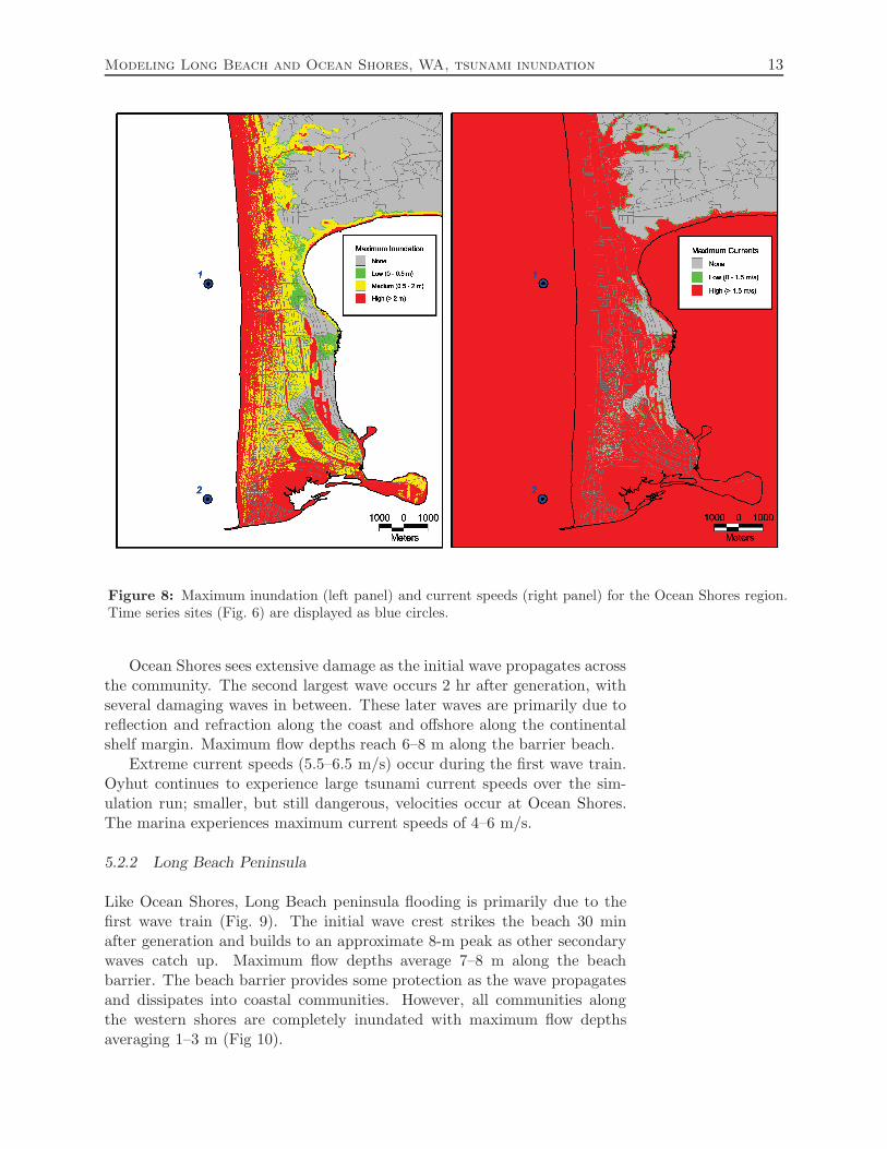
Figure 8: Maximum inundation (left panel) and current speeds (right panel) for the Ocean Shores region.Time series sites (Fig. 6) are displayed as blue circles.

Ocean Shores sees extensive damage as the initial wave propagates acrossthe community. The second largest wave occurs 2 hr after generation, withseveral damaging waves in between. These later waves are primarily due toreflection and refraction along the coast and offshore along the continentalshelf margin. Maximum flow depths reach 6–8 m along the barrier beach.

Extreme current speeds (5.5–6.5 m/s) occur during the first wave train.Oyhut continues to experience large tsunami current speeds over the sim-ulation run; smaller, but still dangerous, velocities occur at Ocean Shores.The marina experiences maximum current speeds of 4–6 m/s.

5.2.2 Long Beach Peninsula

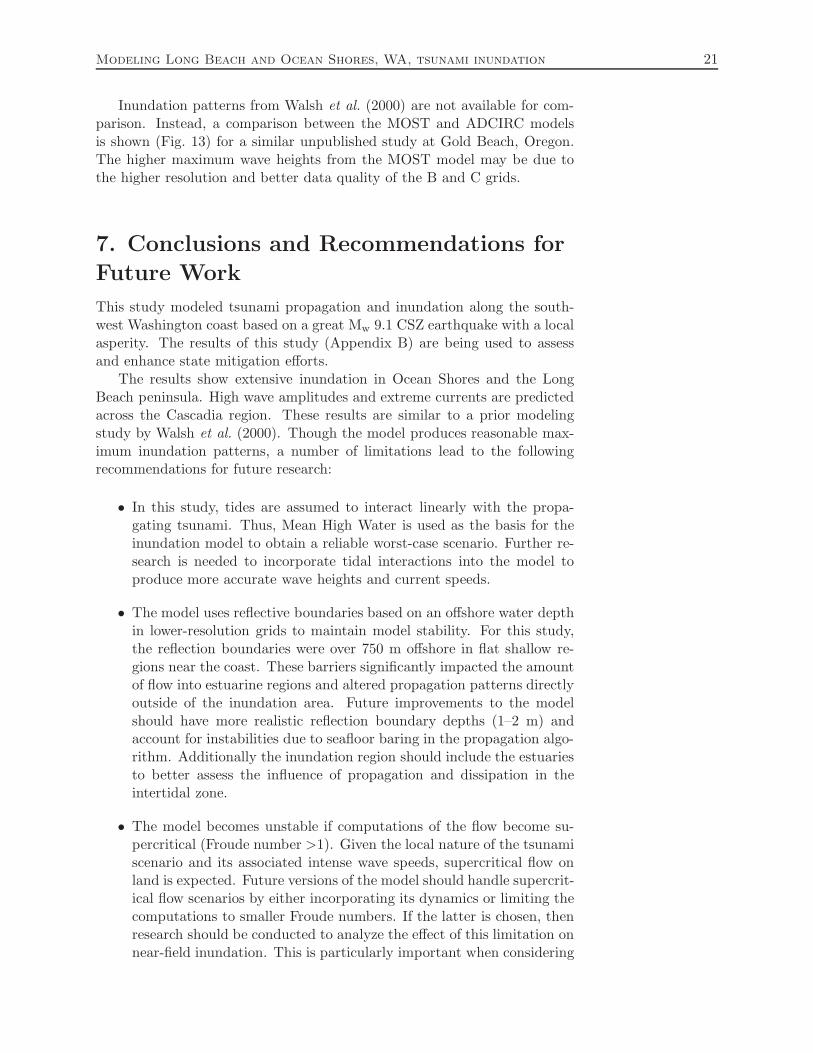
Like Ocean Shores, Long Beach peninsula flooding is primarily due to thefirst wave train (Fig. 9). The initial wave crest strikes the beach 30 minafter generation and builds to an approximate 8-m peak as other secondarywaves catch up. Maximum flow depths average 7–8 m along the beachbarrier. The beach barrier provides some protection as the wave propagatesand dissipates into coastal communities. However, all communities alongthe western shores are completely inundated with maximum flow depthsaveraging 1–3 m (Fig 10).

14 Venturato et al.

Figure 9: Modeled tsunami inundation of the Long Beach peninsula. Snapshots are in 25-min intervals.Wave heights are in meters with respect to Mean High Water.

Extensive inundation also occurs along low-lying regions of the WillapaNational Wildlife Refuge and both major state parks. This simulation showslittle inundation along the eastern coast. Maximum tsunami current speedsreach up to 5 m/s along the barrier beach, and 2.5 m/s at the Port of Ilwaco.

Modeled wave dynamics along the Long Beach peninsula display inter-esting results. The first wave crest has the largest amplitude, but is followedby a relatively minor trough (Fig. 6). The deepest trough (5–6 m) precedesthe second largest wave crest. Thus, the largest tsunami current speeds(4.5–5 m/s) occur approximately 1.8 hr after generation at Ocean Park andOceanside.


Figure 10: Maximum inundation (left panel) and current speeds (right panel) for the Long Beach peninsula.Time series sites (Fig. 6) are displayed as blue circles.

16 Venturato et al.

6. Discussion

6.1 Potential Sources of Error

The MOST model used in this study has been extensively tested againstanalytical solutions, laboratory measurements, and field data (Titov andGonzalez, 1997; Titov and Synolakis, 1998). Since the model performs wellwith all of the benchmark cases described in Synolakis et al. (2007), potentialerrors are limited to the quality of the model initialization parameters, theinitial deformation of the tsunami source, and the DEM.

The setup of the initial conditions for these simulations may producepotentially substantial error in terms of the amount of inundation. As de-scribed in the previous sections, the DEMs were clipped into smaller A, B,and C grids to reduce computational time. The A grid does not cover theentire extent of the initial deformation (Fig. 3). Thus, some of the poten-tial tsunami energy is not being considered. Though this may not affect themaximum inundation from the main energy beam, there are likely additionaleffects from coastal reflection and scattering that are lost.

To stabilize model simulation, the reflection boundaries and inundationdepths for each simulation are different (Table 3). The offshore depth ofthese boundaries may be causing unrealistic wave reflection patterns alongthe outer coast (Fig. 4). This may influence the timing, amplitude, anddirection of later waves.

Additionally, the boundaries of the inundation grid are not adequatelymodeling internal waves in the estuarine regions. This may significantlyaffect the amount and pattern of inundation on land.

Ideally, the C grid would be extended to cover Willapa Bay and GraysHarbor to fully account for the influence of these estuaries on tsunami inun-dation (Fig. 11). Also, the reflection boundaries would be based on a depth(1–2 m) that is much closer to the actual coastline. A new model versionis currently being tested to allow for extended grids and shallow reflectionboundaries.

6.1.1 Limitations of the tsunami source

Tsunami generation depends on the initial deformation of the earthquake.Priest et al. (1997) and the Tsunami Pilot Study Working Group (2006) con-sidered several CSZ deformation scenarios that adequately explore levels ofvariation in line with paleoseismic evidence. However, the next CSZ earth-quake could have a substantially different slip distribution than the mod-eled source and may be associated with tsunamigenic submarine landslides(Goldfinger et al., 1992). Thus, the source represents the largest uncertaintyin the simulation.


Figure 11: Proposed grid extent to reduce potential errors in the model setup.The A grid should be extended to include the entire initial deformation field. TheC grid should be extended to include both Grays Harbor and Willapa Bay.

The location of the asperity within the rupture area has a significanteffect on the directivity of the tsunami energy, and subsequently, on themaximum inundation at Long Beach and Ocean Shores. Priest et al. (1997)saw similar effects when simulating a different asperity further south thatmagnified tsunami energy along the Oregon coast. Other regional asperitieswithin the low-gravity forearc basins should also be investigated to look atthe range of tsunami energy patterns.

6.1.2 Limitations of the DEM

A high quality DEM is necessary to properly model tsunami wave dynamicsand inundation onshore. A number of different factors can contribute toDEM error, including known quantitative errors due to datum conversionand unknown inherent errors produced by combining multiple data sources.Table 4 estimates the total known error for the high-resolution DEM asdescribed in Venturato (2005).

18 Venturato et al.

Table 4: Estimates of root mean square error based on limited known quantitativevalues for the high-resolution model (Venturato, 2005).

Error Type Horizontal Error (m) Vertical Error (m)

Projection/datum conversion range 0.35–0.45 0.05–0.40Comparison with vertical control N/A 0.14–1.80Comparison with original data sources 0.80–10 0.01–1.24Total known quantitative error 1.15–10.45 0.20–3.44

Figure 12: Coverage area of the primary data sources used in the high-resolutionDEM. Sources are labeled with associated survey dates.


Table 5: Comparison of the MOST model and ADCIRC model simulations fromWalsh et al. (2000). Figure 2 displays the locations of time series sites. Waveamplitudes are in meters.

MOST model ADCIRC model

Time Series Site Max. crest Max. trough Max. crest Max. trough

1. Oyhut 5.6 10.0 N/A N/A2. Ocean Shores 6.3 9.3 4.7 6.43. Ocean Park 7.2 5.5 8.8 5.64. Oceanside 8.0 6.3 5.6 4.25. Seaview 7.2 6.1 5.5 3.7

Multiple data sources of various ages were used in the DEM (Fig. 12).Land elevations within the inundation grids are primarily based on recenthigh-resolution LIDAR surveys. U.S. Geological Survey (USGS) surveysfrom the 1970s were used to cover gaps in the topography. Bathymetric datawere primarily taken from recent U.S. Army Corps of Engineers (USACE)surveys and much older NOS hydrographic surveys.

Though the DEM is based on the best available data in the region, it maynot accurately reflect nearshore water depths. The age of the surveys in thenearshore coastal region are too old to reflect the significant changes of theColumbia River littoral zone. As described in the Study Area section, recenterosion trends have deepened the water offshore of these beach barriers. It isunclear how much error is introduced by using these older surveys. In orderto accurately address this issue, high-resolution multibeam surveys shouldbe conducted.

6.2 Model Comparison

This modeling study is an update to a prior effort that used a finite elementmodel known as ADCIRC (Walsh et al., 2000). Both studies used the sameinitial deformation scenario, but this study implements an updated DEM.

As discussed in previous sections, this study’s high-resolution DEM in-cludes very accurate LIDAR topography and updated bathymetry withinthe estuarine regions. The 2000 study used topography from 1973 USGSsurveys (Priest et al., 1997). The 6- to 10-m topographic contours fromthe USGS surveys do not cover the intricate details of the low-lying inunda-tion areas. Significant coastal changes have also occurred along the barrierbeaches over the past 30 years. Additionally, the 2000 DEM did not applya standard vertical datum for all data sources leading to a 2- to 6-m verticalerror range (Walsh et al., 2000).

Table 5 shows the comparison between maximum wave crests and troughsbased on specified time series locations (Fig. 2). The values for the ADCIRCmodel were estimated from graphics in Walsh et al. (2000). The MOSTmodel produces higher maximum wave heights at all site locations exceptOcean Park. Both studies predict that the first wave is the largest, and laterwaves occur at similar times.

20 Venturato et al.

[m]

0.1.

2.3.

4.5.

6.7.

8.9.

10.

MO

ST

Fin

ite D

iffer

ence

Mod

el

[m]

0.1.

2.3.

4.5.

6.7.

8.9.

10.

AD

CIR

C F

inite

Ele

men

t Mod

el

[m]

-10.

-8.

-6.

-4.

-2.

0.2.

4.6.

8.10

.

Diff

eren

ce, A

DC

IRC

–MO

ST

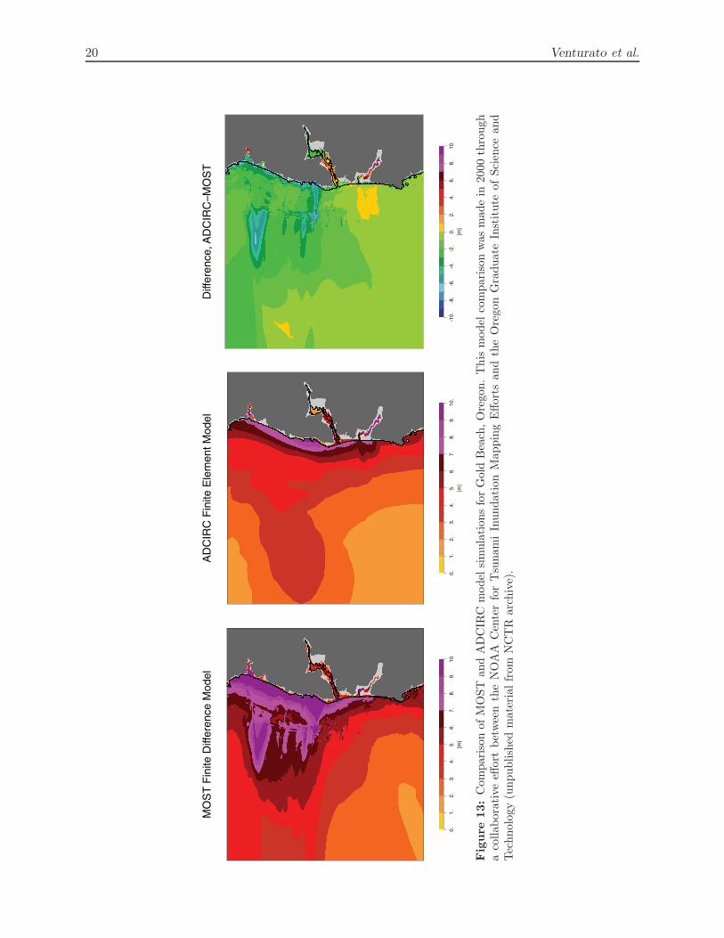
Fig

ure

13:

Com

pari

son

ofM

OST

and

AD

CIR

Cm

odel

sim

ulat

ions

for

Gol

dB

each

,Ore

gon.

Thi

sm

odel

com

pari

son

was

mad

ein

2000

thro

ugh

aco

llabo

rati

veeff

ort

betw

een

the

NO

AA

Cen

ter

for

Tsu

nam

iIn

unda

tion

Map

ping

Effo

rts

and

the

Ore

gon

Gra

duat

eIn

stit

ute

ofSc

ienc

ean

dTec

hnol

ogy

(unp

ublis

hed

mat

eria

lfro

mN

CT

Rar

chiv

e).


Inundation patterns from Walsh et al. (2000) are not available for com-parison. Instead, a comparison between the MOST and ADCIRC modelsis shown (Fig. 13) for a similar unpublished study at Gold Beach, Oregon.The higher maximum wave heights from the MOST model may be due tothe higher resolution and better data quality of the B and C grids.

7. Conclusions and Recommendations for

Future Work

This study modeled tsunami propagation and inundation along the south-west Washington coast based on a great Mw 9.1 CSZ earthquake with a localasperity. The results of this study (Appendix B) are being used to assessand enhance state mitigation efforts.

The results show extensive inundation in Ocean Shores and the LongBeach peninsula. High wave amplitudes and extreme currents are predictedacross the Cascadia region. These results are similar to a prior modelingstudy by Walsh et al. (2000). Though the model produces reasonable max-imum inundation patterns, a number of limitations lead to the followingrecommendations for future research:

• In this study, tides are assumed to interact linearly with the propa-gating tsunami. Thus, Mean High Water is used as the basis for theinundation model to obtain a reliable worst-case scenario. Further re-search is needed to incorporate tidal interactions into the model toproduce more accurate wave heights and current speeds.

• The model uses reflective boundaries based on an offshore water depthin lower-resolution grids to maintain model stability. For this study,the reflection boundaries were over 750 m offshore in flat shallow re-gions near the coast. These barriers significantly impacted the amountof flow into estuarine regions and altered propagation patterns directlyoutside of the inundation area. Future improvements to the modelshould have more realistic reflection boundary depths (1–2 m) andaccount for instabilities due to seafloor baring in the propagation algo-rithm. Additionally the inundation region should include the estuariesto better assess the influence of propagation and dissipation in theintertidal zone.

• The model becomes unstable if computations of the flow become su-percritical (Froude number >1). Given the local nature of the tsunamiscenario and its associated intense wave speeds, supercritical flow onland is expected. Future versions of the model should handle supercrit-ical flow scenarios by either incorporating its dynamics or limiting thecomputations to smaller Froude numbers. If the latter is chosen, thenresearch should be conducted to analyze the effect of this limitation onnear-field inundation. This is particularly important when considering

22 Venturato et al.

potential vertical evacuation strategies, such as calculating forces onstructures.

• Multibeam bathymetric surveys should be conducted offshore of Wash-ington and northern Oregon. This work could significantly reduce er-rors in the model and provide a better picture of seafloor changes inthe Columbia River littoral cell.

• Prior work by Doyle (1996) suggest that abrupt tectonic subsidencefrom a large CSZ earthquake would cause 200–400 m of catastrophicbeach retreat throughout the Columbia River littoral cell. An inter-esting research project would incorporate the modeled wave dynamicsfrom this study with a shoreface translation model to determine theeffect of tsunami waves on beach recession and subsequent alterationsto sediment transport patterns within the littoral cell.

• This modeling study considered a credible worst-case scenario in thenear field. After the devastating 26 December 2004 Boxing Daytsunami, many scientists have taken another look at the potentialfault dynamics of the CSZ. Several new earthquake scenarios have beendeveloped (Tsunami Pilot Study Working Group, 2006). Additionalmodel scenarios should be run to determine whether the one used inthis study remains the most credible worst case. Far-field scenarios arealso being considered to help emergency managers consider potentiallymultiple evacuation strategies that are dependent on the event type.

Acknowledgments. This research was funded by the National Tsunami HazardMitigation Program via a grant from the Washington State Military DepartmentEmergency Management Division. This publication is partially funded by the JointInstitute for the Study of the Atmosphere and Ocean (JISAO) under NOAA Coop-erative Agreement No. NA17RJ1232, Contribution #1337.

The authors thank George Crawford, Tim Walsh, George Priest, and LonnieReid-Pell for assistance with data sources and processing. The authors also thankHal Mofjeld and Mick Spillane for assisting with water-level datum issues and ver-ifying the Gaussian distribution for the earthquake asperity. Utku Kanoglu alsoexpresses his gratitude to the Pacific Marine Environmental Laboratory for finan-cial support during his summer 2005 visit.


8. References

Atwater, B.F. (1987): Evidence for great Holocene earthquakes along the outercoast of Washington State. Science, 336, 942–944.

Atwater, B.F., A.R. Nelson, J.J. Clague, G.A. Carver, D.K. Yamaguchi, P.T. Bo-browski, J. Bourgeois, M.E. Darienzo, W.C. Grant, E. Hemphill-Haley, H.M.Kelsey, G.C. Jacoby, S.P. Nishenko, S.P. Palmer, C.D. Peterson, and M.A.Reinhart (1995): Summary of coastal geologic evidence for past great earth-quakes at the Cascadia subduction zone. Earthq. Spectra, 11 (1), 1–18.

Doyle, D.L. (1996): Beach response to subsidence following a Cascadia subductionzone earthquake along the Washington-Oregon coast. M.S. thesis, PortlandState University, Portland, OR, 113 pp.

Goldfinger, C., L.D. Kulm, R.S. Yeats, C. Mitchell, R.E. Weldon, III, C.D. Peterson,M.E. Darienzo, W. Grant, and G. Priest (1992): Neotectonic map of the Oregoncontinental margin and adjacent abyssal plain. Oregon Department of Geologyand Mineral Industries Open-File Report O-92-4, 17 pp.

Grays Harbor County (2005): Grays Harbor County statistical information. http://www.co.grays-harbor.wa.us/

Kaminsky, G.M., M.C. Buijsman, G. Gelfenbaum, P. Ruggiero, H.M. Jol, A.E.Gibbs, and C.D. Peterson (1999): Synthesizing geological observations andprocesses-response data for modeling coastal change at management scale. InProceedings of Coastal Sediments 99, ASCE, 1708–1723.

Mofjeld, H.O., M.G.G. Foreman, and A. Ruffman (1997): West Coast tides duringCascadia Subduction Zone tsunamis. Geophys. Res. Lett., 24 (17), 2215–2218.

Mofjeld, H.O., F.I. Gonzalez, V.V. Titov, A.J. Venturato, and J.C. Newman (2007):Effects of tides on maximum tsunami wave heights: Probability distributions.J. Atmos. Ocean. Tech., 24 (1), 117–123.

Mofjeld, H.O., V.V Titov, F.I. Gonzalez , and J.C. Newman (2000): Analytictheory of tsunami wave scattering in the open ocean with application to theNorth Pacific. NOAA Tech. Memo. OAR PMEL-116, NTIS: PB2002-101562,NOAA/Pacific Marine Environmental Laboratory, Seattle, WA, 38 pp.

Mofjeld, H.O., A.J. Venturato, F.I. Gonzalez , and V.V. Titov (2004): Backgroundtides and sea level variations at Seaside, Oregon. NOAA Tech. Memo. OARPMEL-126, NTIS: PB2005-100990, NOAA/Pacific Marine Environmental Lab-oratory, Seattle, WA, 15 pp.

Myers, E.P., III, A.M. Baptista, and G.R. Priest (1999): Finite element modelingof potential Cascadia subduction zone tsunamis. Science of Tsunami Hazards,17 (1), 3–18.

National Science and Technology Council (2005): Tsunami risk reduction for theUnited States: A framework for action. Joint Report of the Subcommittee onDisaster Reduction and the U.S. Group on Earth Observations, 30 pp.

Ocean Shores Chamber of Commerce (2005): Ocean Shores Visitor Guide, OceanShores, Washington. http://oceanshores.org/

Pacific County (2003): Pacific County statistical information. http://www.co.pacific.wa.us/

Petersen, M.D., C.H. Cramer, and A.D. Frankel (2002): Simulations of seismic haz-ard for the Pacific Northwest of the United States from earthquakes associatedwith the Cascadia subduction zone. Pure Appl. Geophys., 159 (9), 2147–2168.

Peterson, C.D., G. Gelfenbaum, H.M. Jol, J.B. Phipps, F. Reckendorf, D.C. Twichell,S. Vanderburgh, and L. Woxell (1999): Great earthquakes, abundant sand, and

24 Venturato et al.

high wave energy in the Columbia cell, USA. In Proceedings of Coastal Sedi-ments 99, ASCE, 1676–1691.

Priest, G.R., E.P. Myers III, A.M. Baptista, P. Fleuck, K. Wang, R.A. Kamphaus,and C.D. Peterson (1997): Cascadia subduction zone tsunamis—Hazard map-ping at Yaquina Bay, Oregon. Oregon Department of Geology and MineralIndustries Open-File Report O-97-34, 144 pp.

Satake, K., K. Shimazaki, Y. Tsuji, and K. Ueda (1996): Time and size of a greatearthquake in Cascadia inferred from Japanese tsunami records of January1700. Nature, 379 (6562), 246–249.

Synolakis, C.E., E.N. Bernard, V.V. Titov, U. Kanoglu, and F.I. Gonzalez (2007):Standards, criteria, and procedures for NOAA evaluation of tsunami numer-ical models. NOAA Tech. Memo. OAR PMEL-135, NOAA/Pacific MarineEnvironmental Laboratory, Seattle, WA, 55 pp.

Titov, V.V., and F.I. Gonzalez (1997): Implementation and testing of the Methodof Splitting Tsunami (MOST) model. NOAA Tech. Memo. ERL PMEL-112, NTIS: PB98-122773, NOAA/Pacific Marine Environmental Laboratory,Seattle, WA, 11 pp.

Titov,V.V., F.I. Gonzalez, H.O. Mofjeld, and A.J. Venturato (2003): NOAA TIMESeattle tsunami mapping project: Procedures, data sources, and products.NOAA Tech. Memo. OAR PMEL-124, NTIS: PB2004-101635, NOAA/PacificMarine Environmental Laboratory, Seattle, WA, 21 pp.

Titov, V.V., and C.E. Synolakis (1998): Numerical modeling of tidal wave runup.J. Waterw. Port Coast. Ocean Eng., 124 (4), 157–171.

Tsunami Pilot Study Working Group (2006): Seaside, Oregon Tsunami Pilot Study—Modernization of FEMA flood hazard maps. NOAA OAR Special Report,NOAA/OAR/PMEL, Seattle, WA, 94 pp.

Venturato, A.J. (2005): A digital elevation model for Seaside, Oregon: Procedures,data sources, and analyses. NOAA Tech. Memo. OAR PMEL-129, NTIS:PB2006-101562, NOAA/Pacific Marine Environmental Laboratory, Seattle, WA,17 pp.

Walsh, T.J., C.G. Caruthers, A.C. Heinitz, E.P. Myers III, A.M. Baptista, G.B.Erdakos, and R.A. Kamphaus (2000): Tsunami hazard map of the southernWashington Coast: Modeled tsunami inundation from a Cascadia subductionzone earthquake. Washington Division of Geology and Earth Resources Geo-logic Map GM-49, 3–12.

Washington State Department of Ecology (2007): Washington State Coastal Haz-ards. http://www.ecy.wa.gov/programs/sea/coast/hazards.html

Wells, R.E., R.J. Blakely, Y. Sugiyama, D.W. Scholl, and P.A. Dinterman (2003):Basin-centered asperities in great subduction zone earthquakes: A link betweenslip, subsidence, and subduction erosion? J. Geophys. Res., 108 (B10), 2507–2537.

Woxell, L.K. (1998): Prehistoric beach accretion rates and long-term response tosediment depletion in the Columbia River Littoral System, USA. M.S. thesis,Portland State University, Portland, OR, 206 pp.

Yamaguchi, D.K., B.F. Atwater, D.E. Bunker, B.E. Benson, and M.S. Reid (1997):Tree-ring dating in the 1700 Cascadia earthquake. Nature, 389 (6654), 922–924.


Appendix A: Data Credit

NOAA Coastal Services Center, Coastal Remote Sensing Program (2004):Aircraft Laser/GPS mapping of coastal topography. Charleston, SouthCarolina. http://www.csc.noaa.gov/lidar/

NOAA National Geodetic Survey (2004): Vertical geodetic control data.Silver Spring, Maryland. http://www.ngs.noaa.gov/

NOAA National Geophysical Data Center (2002): NOS HydrographicDatabase, GEODAS Version 4.1.18. Boulder, Colorado. http://ngdc.noaa.gov/

NOAA National Ocean Service (2004): Regional water-level station bench-marks. Silver Spring, Maryland. http://tidesandcurrents.noaa.gov/benchmarks/

Oregon Bureau of Land Management (2001): Oregon Watershed Boundaries.Portland, Oregon. Data obtained through the Oregon Geospatial DataClearinghouse. http://www.gis.state.or.us/

U.S. Army Corps of Engineers (2004): Hydrographic surveys for ColumbiaRiver, Grays Harbor, and Willapa Bay. Portland, Oregon and Seattle,Washington. http://www.nwp.usace.army.mil/

U.S. Geological Survey EROS Data Center (1999): National ElevationDataset. Sioux Falls, South Dakota. http://gisdata.usgs.net/ned/

U.S. Geological Survey National Aerial Photography Program (2002): 2000Digital Orthophoto Quads. Reston, Virginia. Data obtained throughthe Oregon Geospatial Data Clearinghouse. http://www.gis.state.or.us/

Washington State Department of Ecology (2001): Washington State marineshorelines. Olympia, Washington. http://www.ecy.wa.gov/services/gis/

26 Venturato et al.

Appendix B: Modeling Products

Model results (Table B.1) were provided to two Washington State agen-cies, the Military Department Emergency Management Division and theDivision of Geology and Earth Resources, for use in tsunami hazard map-ping and mitigation. All geospatial data were provided in ASCII raster orESRI ArcGIS© formats. Animations were provided in QuickTime© format.These state agencies are responsible for redistribution of these data.

Table B.1: Tsunami model products.

Name Type

animations QuickTime movies depicting tsunami wave evolution and am-plitudes

documentation Modeling product report and presentationsgis Geospatial representation of model results and DEMs in ESRI

ArcGIS©and ASCII raster formatsimages Images of model resultsmetadata Information related to each datasettimeseries Spreadsheet of model time series for specific sites along the

Washington coast

MODELING TSUNAMI INUNDATION FROM A … tsunami inundation from a cascadia subduction zone earthquake...

Documents

Transcript of MODELING TSUNAMI INUNDATION FROM A … tsunami inundation from a cascadia subduction zone earthquake...