Modeling the Relationship Between Vehicle Speed and...

Modeling the Relationship Between Vehicle Speed and Fuel Consumption

Wednesday, March 14, 20182:00-3:30 PM ET

TRANSPORTATION RESEARCH BOARD

The Transportation Research Board has met the standards and

requirements of the Registered Continuing Education Providers Program.

Credit earned on completion of this program will be reported to RCEP. A

certificate of completion will be issued to participants that have registered

and attended the entire session. As such, it does not include content that

may be deemed or construed to be an approval or endorsement by RCEP.

Purpose Discuss the relationship between vehicle speed and fuel economy as investigated by the U.S. Federal Highway Administration.

Learning ObjectivesAt the end of this webinar, you will be able to:

• Apply developed prediction models to estimate vehicle fuel consumption as a function of road grade level

• Assess the influence of traffic congestion level on fuel consumption• Assess the influence of the number of signalized intersections on fuel

consumption• Assess the excess in fuel consumption due to road curvatures

Slide No. 1

Modeling the Relationship Between Vehicle Speed & Fuel Consumption

TRB WebinarMarch 14, 2018

Slide No. 2

Acknowledgment

• U.S. DOT, FHWA DTFH61-14-C-00044: Enhanced Prediction of Vehicle Fuel Economy and Other Vehicle Operating Costs.

• American Transportation Research Institute (ATRI) for its support.

Disclaimer: The contents reflect the views of the authors, who are responsible for the facts and accuracy of the information presented herein. This webinar is disseminated under the sponsorship of the U.S. Department of Transportation, FHWA in the interest of information exchange. The U.S. Government assumes no liability for the contents or use thereof.

Slide No. 3

Abbreviations

• AS: Average Speed in mph

• GR: Road Grade in percent (UGR upgrade, DGR: Downgrade)

• GRlevel: Road Grade level (level A through F)

• SL: Speed Limit in mph

• NTCD: Number of Traffic Control Devices per mile (Average) (positive real number)

• FAC: Full Access Control facilities

• PNAC: Partial or No Access Control facilities

• LOS: Level Of Service

• DCA: Degree of curvature in degrees

• IRI: international Roughness Index

• PSD: Power Spectral Density

• PCAF: Pavement Condition Adjustment Factor

Slide No. 4

Overall Project Objective

• “…to improve the state-of-the-art in vehicle operating costs (VOC) estimation for use in benefit cost analysis.”– Vehicle Fuel Economy (FE)

– Non-Fuel Vehicle Operating Costs (VOC):Tire WearOil ConsumptionRepair and MaintenanceMileage-Related Vehicle Depreciation

– Considerations to changes in vehicle technology, vehicle operating speeds, traffic management & driving cycles.

Slide No. 5

Project Team Organization

Federal Highway AdministrationMr. Matthew A. Phelps, CO

Mr. Valentin Vulov, COR

Principal Investigators (university of Nevada, Reno)Dr. Elie Y. Hajj (PI)

Dr. Peter E. Sebaaly, P.E. (Co-PI)

University of Nevada, Reno

Traffic Engineering (Operations & Simulations)

Hao XuZong Tian

Pavement Engineering/Vehicle-Pavement Interaction

Elie Y. HajjRami Chkaiban

Seyed-Farzan KazemiPeter E. Sebaaly

Nevada Automotive Test Center

Vehicle Modeling & Simulations/Fuel Economy

Muluneh SimeGary Bailey

Dynatest Consulting

Non-Destructive Pavement Testing & Characteristics

Alvaro UlloaPer Ullidtz

Gabriel Bazi

Contracts ManagerMs. Charlene Hart, MBA, CPA,

CFE, CRA

Slide No. 6

OVERALL SCOPESection A, Elie Y. Hajj

Slide No. 7

PHASE I

PHASE I: MODELING THE RELATIONSHIP

BETWEEN VEHICLE SPEED

AND FUEL

Driving Cycle Development for Roadways

with Full Access Control (FAC)

Fuel Consumption

(FC) Estimates for FAC

Driving Cycle Development for Roadways with Partial or

No Access Control (PNAC)

Fuel Consumption

(FC) Estimates for PNAC

Source: TxDOT, Transportation Planning & Programming Division

Full Access Control (FAC); all access via grade-separated interchanges

Partial Control; access via grade-separated interchanges & direct access roadways

No Access Control

Source: FDOT RCI Field Handbook, Nov. 2008.

Source: TxDOT, Transportation

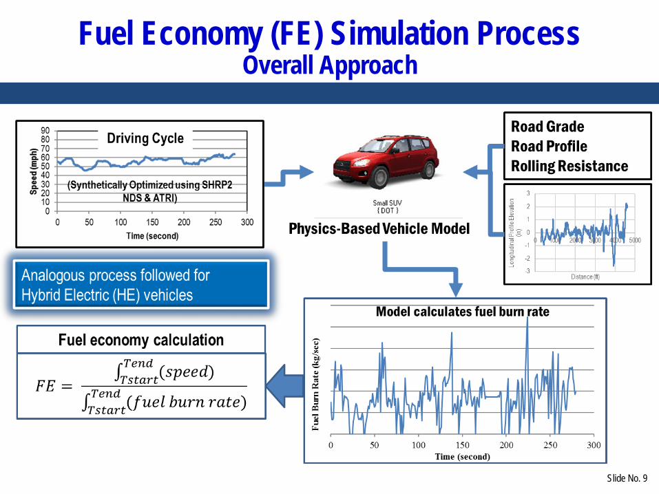
FE = f(AS, GR, SL, NTCD)

Slide No. 8

PHASE II

MODELING THE RELATIONSHIP BETWEEN PAVEMENT ROUGHNESS, SPEED,

ROADWAY CHARACTERISTICS AND VEHICLE OPERATING COSTS

Effects of Road Curvature on Fuel Consumption

Incremental Fuel Consumption Due to

Pavement Roughness

Effects of Infrastructure Physical & Operating

Characteristics on Non-Fuel Vehicle Operating

Costs (VOC)

Slide No. 9

Fuel Economy (FE) Simulation ProcessOverall Approach

Slide No. 10

DRIVING CYCLESSection B, Hao Xu

Slide No. 11

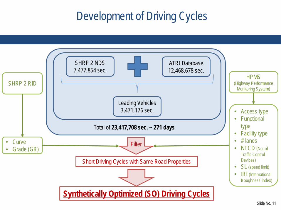
Development of Driving Cycles

SHRP 2 NDS7,477,854 sec.

ATRI Database12,468,678 sec.

Leading Vehicles3,471,176 sec.

Total of 23,417,708 sec. ~ 271 days

Filter

SHRP 2 RIDHPMS

(Highway Performance Monitoring System)

Short Driving Cycles with Same Road Properties

• Curve• Grade (GR)

• Access type• Functional

type• Facility type• # lanes• NTCD (No. of

Traffic Control Devices)

• SL (speed limit)• IRI (International

Roughness Index)

Synthetically Optimized (SO) Driving Cycles

Slide No. 12

Road Scenarios

• 45 full access control (FAC) scenarios.– 15 rural scenarios and 30 urban scenarios;– Horizontal curve level A; – Grade levels of A through C.

• 335 partial or no access control (PNAC) scenarios.– 186 rural scenarios and 149 urban scenarios;– Horizontal curve levels of A and B;– Grade levels of A through D.

• In all cases travel length longer than 5 miles was targeted.

Slide No. 13

Road ScenariosTraffic Condition and Up/Down Grade

• Traffic condition: level of service (LOS)– Average travel speed of each trip snippet was calculated Total travel distance divided by total travel time

– Convert average travel speeds to traffic LOS

• Upgrade & downgrade condition– Same HPMS grade includes up & down situations– Elevation change of each trip snippet was used to determine the upgrade or

downgrade– Driving cycles for upgrade & downgrade situations were considered

separately.

Slide No. 14

Data: SHRP 2 Naturalistic Driving Study (NDS) Driver Age & Vehicle Distributions

• 4,400-trip SHRP 2 NDS data– 6 NDS data collections sites of 6 states

(urban/rural).– Each trip is ≥ 20-min– 7,477,854-sec data of NDS vehicles

5.6%

71.1%

18.7%4.6%

0%20%40%60%80%

100%

Freq

uenc

y Per

cent

age i

n Re

ceive

d ND

S Tr

ips

Vehicle Types

Vehicle type distribution of the 4,400 NDS trips

0%

5%

10%

15%

20%

1987

1988

1989

1990

1991

1992

1993

1994

1995

1996

1997

1998

1999

2000

2001

2002

2003

2004

2005

2006

2007

2008

2009

2010

2011

2012

2013Pe

rcen

tage

in R

eceiv

ed

NDS

Trip

s

Vehicle Year

Vehicle year distribution of the 4,400 NDS trips

Note: the leading vehicle information not included in the charts.

0%2%4%6%8%

10%12%

16-1

920

-24

25-2

930

-34

35-3

940

-44

45-4

950

-54

55-5

960

-64

65-6

970

-74

75-7

980

-84

85+

Perc

enta

ge o

f Pop

ulat

ion

of

Inte

rest

Age Group (years)SHRP 2 Participants (Trips for Driving Cycle Development)U.S. Licensed Drivers (2014)

Driver age distribution of the 4,400 NDS trips

Slide No. 15

DataAmerican Transportation Research Institute (ATRI) Truck Data

• Combination truck data were obtained from ATRI– ATRI offered a heavily subsidized agreement & support.– Truck trips collected in Seattle WA, Tampa FL & Buffalo NY (3 of the 6 NDS data

collection sites).– 12,468,678-second truck data records.– Trip data were collected for 2 weeks in October 2015.

10,641,702sec., 85%

1,826,976sec., 15%

UrbanRural

Slide No. 16

DataLeading Vehicle Data Processing

• NDS (Naturalistic Driving Study) leading vehicle data extraction:– Using NDS front videos and radar data: the distance range & rate of range change between a

NDS vehicle and the leading vehicle.– Method was used in CARB/Sierra 2004 Sacramento Ramp Driving & Caltrans/CARB 2000

California Route Driving studies.– A tool was developed to synchronize the front video and NDS data.– Total of 3,246,160-second radar data from 46,281 trip snippets.

User interface of the NDS Front Video Review Tool. Sample of a NDS front video frame.

Large light duty vehicle

Slide No. 17

Driving Cycle DevelopmentSynthetic Optimization (SO) – Flow Chart

• Better representing the driving pattern of total trip samples

• Second-by-second change of speed & acceleration is actually observed in trip samples.

• Minimize the impact of possible map-matching errors in trip snippets.

SAFD (Speed-Acceleration Frequency Distribution)

SATM (Speed-Acceleration Transition Matrix)

SA (Simulated Annealing)

Slide No. 18

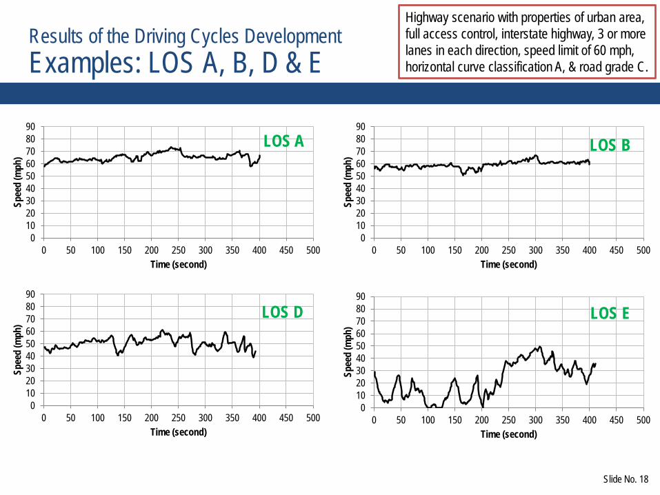
Results of the Driving Cycles DevelopmentExamples: LOS A, B, D & E

Highway scenario with properties of urban area, full access control, interstate highway, 3 or more lanes in each direction, speed limit of 60 mph, horizontal curve classification A, & road grade C.

0102030405060708090

0 50 100 150 200 250 300 350 400 450 500

Spee

d (m

ph)

Time (second)

LOS A

0102030405060708090

0 50 100 150 200 250 300 350 400 450 500

Spee

d (m

ph)

Time (second)

LOS B

0102030405060708090

0 50 100 150 200 250 300 350 400 450 500

Spee

d (m

ph)

Time (second)

LOS D

0102030405060708090

0 50 100 150 200 250 300 350 400 450 500

Spee

d (m

ph)

Time (second)

LOS E

Slide No. 19

Results of the Driving Cycles DevelopmentOverall Summary of Developed Driving Cycles

• Comprehensive dataset for driving cycles.– SHRP 2 RID– SHRP 2 NDS– USGS NED– ATRI truck data

• 654 unique synthetic optimization (SO) driving cycles.– 212 driving cycles for Full Access Control (FAC) Highway.– 442 driving cycles for Partial or No Access Control (PNAC) Highway.

• Driving cycles are next used as input for fuel economy simulations.

Example of USGS NED data

Slide No. 20

VEHCILE SIMULATION MODELSSection C, Muluneh Sime

Slide No. 21

Full Vehicle Models

• Physics-based models built to represent a range of vehicles

• Each simulation model consists of 4 subsystems:– Chassis, including tires, suspension, aero

& rolling resistance loads– Power train, including engine,

transmission, differentials, accessories, & control systems

– Roads, including grades, curves, & roughness

– Driving cycles, i.e., speed as a function of time

Slide No. 22

Physics-Based Vehicle Models20 Vehicle Chassis

Small light duty vehicles(6 SLD vehicles)

Subcompact Compact

Mid size sedanLarge sedanSmall SUV

Minivan

Large light duty vehicles (5 LLD vehicles)

Small PickupLarge SUV

Class 1 truckClass 2 truck

Commuter van

Busses(3 vehicles)School bus

City busLong distance busTwo axle trucks with dual

rear tires(3 vehicles)Class 3 truckClass 4 truckClass 5 truck

Truck with 3 axles (1 vehicle)

Vocational Dump Truck(Gravel truck)

Combination trucks(2 vehicles)Tractor trailer

Slide No. 23

Simulated Vehicle Fleet

• 30 vehicles simulated (20 chassis with different engine types)• Gasoline• Diesel• Gasoline-Ethanol

blend of up to 85% ethanol (E85)

• Hybrid-Electric (HE)• Liquid Natural Gas

(LNG).

Slide No. 24

Vehicle Simulation Model Verification

• Verification Effort: Simulate vehicle operation on known speed cycles and compare simulated fuel economy with measured data.

• Three sources of data used:

–LDV (light duty vehicles) data for EPA drive cycles is published data. Sample vehicle models were run for city, highway, & combined drive cycle fuel economy.

–Two axle, 6 wheel truck data was obtained through physical testing.

–Class 8 truck data obtained from Oak Ridge National Labs (ORNL).

Slide No. 25

Light Duty Vehicle (LDV) Model Verification Results

05

1015202530354045

0 5 10 15 20 25 30 35 40 45

Sim

ulat

ed F

uel E

cono

my (

mpg

)

Sample Vehicle Fuel Economy (mpg)City Highway CombinedLine of Equality +10 percent -10 percent

Slide No. 26

Vehicle Model Verification Example: Class 5 Truck

• Instrument a test vehicle & operate over a range of drive cycles & road grades

• Create simulation environment for virtual testing

• Compare model & test results32.8 mile routeTest Vehicle: 10.9 mpg | Simulation Vehicle: 11.1 mpgDifference in mpg = 1.8 %

Slide No. 27

Vehicle Model Verification Example: Class 8 Truck

• Data obtained from Oak Ridge National Laboratories– Heavy Truck Duty Cycle (HTDC) project sponsored by the US Department of Energy’s

(DOE’s) Office of Freedom Car and Vehicle Technologies.– Test cycle was 764 miles– Vehicle weight 53,000 lb– Test results: 5.0 mpg | Simulation result: 4.95 mpg

Slide No. 28

Road Conditions: Grades

• Phase I considered only smooth surface pavements with no curvatures (i.e., straight).

• Upslope (+) & downslope (-) grades are included (12 grades total).

Road Grade Classification (GRlevel)

Grade (%) Grade Used in Simulations (%)

A 0.0 – 0.4 ±0.20B 0.5 – 2.4 ±1.45C 2.5 – 4.4 ±3.45D 4.5 – 6.4 ±5.45E 6.5 – 8.4 ±7.45F 8.5 or greater ±10.0

Slide No. 29

Road Conditions: Curvatures

• Phase II considered influence of road curvature on fuel economy (smooth pavement).

Curve Level

Radius of Curve, R (ft) Radius Value Used in Vehicle Simulations (ft)

Degrees of curvature, DCA, Used in Vehicle

Simulations (°)Min MaxA 1,637 Straight Straight 0.0B 1,061 1,637 1,349 4.25C 682 1,061 871.5 6.58D 412 682 547 10.48E 205 412 308.5 18.58F 0 205 102.5 55.90

Slide No. 30

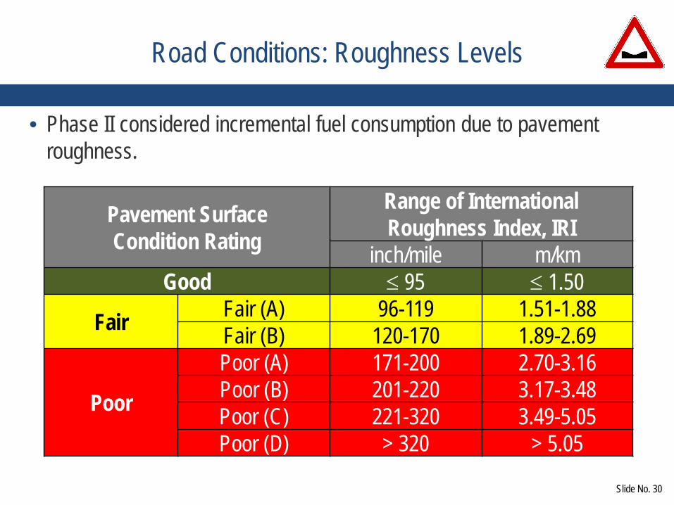
Road Conditions: Roughness Levels

• Phase II considered incremental fuel consumption due to pavement roughness.

Pavement Surface Condition Rating

Range of International Roughness Index, IRI

inch/mile m/kmGood ≤ 95 ≤ 1.50

Fair Fair (A) 96-119 1.51-1.88Fair (B) 120-170 1.89-2.69

Poor

Poor (A) 171-200 2.70-3.16Poor (B) 201-220 3.17-3.48Poor (C) 221-320 3.49-5.05Poor (D) > 320 > 5.05

Slide No. 31

Spatial Power Spectral Density (PSD) for Selected Roughness Levels

• PSD defines both amplitude & frequency characteristics of the rough pavement.

• Visualization of the relative differences in pavement roughness between classifications of pavement surface conditions.

Increase in pavement roughness levels

Slide No. 32

Rolling Resistance (RR) Components

• Rolling resistance is assumed to consist of 3 components– Rolling resistance of a tire on a smooth surface– Additional rolling resistance force of the tire due to pavement roughness– Additional rolling resistance due to suspension power dissipation

0.0000

0.0020

0.0040

0.0060

0.0080

0.0100

0.0120

0 20 40 60 80 100

Rollin

g Re

sista

nce C

oeffi

cient

, RR

C

Speed (mph)

GoodFair (A)Fair (B)Poor (A)Poor (B)Poor (C)Poor (D)

Subcompact Car Example Results• Rolling resistance

force is a function of pavement roughness amplitude & frequency content

Increase in pavement roughness levels

Slide No. 33

Fuel Economy (FE) Simulations

• 30 vehicle models were run using speed cycles & defined road characteristics to calculate fuel economy.

• Smooth straight roads with +/- grades– 15,516 simulations

• Smooth roads with curvatures & +/- grades– 34,822 simulations

• Straight roads with a range of roughness levels & zero grade– 1,890 simulations

Over 52,000 simulations

Slide No. 34

FUEL ECONOMY (FE) PREDICTION MODELSSection D, Elie Y. Hajj

Slide No. 35

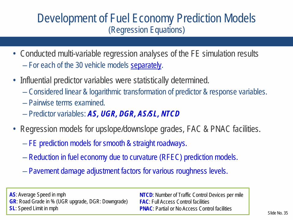
Development of Fuel Economy Prediction Models (Regression Equations)

• Conducted multi-variable regression analyses of the FE simulation results – For each of the 30 vehicle models separately.

• Influential predictor variables were statistically determined.– Considered linear & logarithmic transformation of predictor & response variables.– Pairwise terms examined. – Predictor variables: AS, UGR, DGR, AS/SL, NTCD

• Regression models for upslope/downslope grades, FAC & PNAC facilities. – FE prediction models for smooth & straight roadways.– Reduction in fuel economy due to curvature (RFEC) prediction models.– Pavement damage adjustment factors for various roughness levels.

AS: Average Speed in mphGR: Road Grade in % (UGR upgrade, DGR: Downgrade)SL: Speed Limit in mph

NTCD: Number of Traffic Control Devices per mileFAC: Full Access Control facilitiesPNAC: Partial or No Access Control facilities

Slide No. 36

Fuel Economy Prediction ModelsFull Access Control (FAC) – Upslope Grade, Large Sedan, Gasoline

0

10

20

30

40

50

0 20 40 60 80 100

Fuel

Econ

omy (

mpg

)

Average Speed (mph)

SLDV (LargeSedan_gas) Upslope_Grade_ADriving Cycles_AverageDriving Cycles_SegmentedSteady StatePrediction Model

0

10

20

30

40

50

0 20 40 60 80 100

Fuel

Econ

omy (

mpg

)

Average Speed (mph)

SLDV (LargeSedan_gas) Upslope_Grade_BDriving Cycles_AverageDriving Cycles_SegmentedSteady StatePrediction Model

21.1

32.0

17.0

24.4

Slide No. 37

Fuel Economy Prediction ModelsFull Access Control (FAC) – Downslope Grade, Large Sedan, Gasoline

0

20

40

60

80

100

0 20 40 60 80 100

Fuel

Econ

omy (

mpg

)

Average Speed (mph)

SLDV (LargeSedan_gas) Downslope_Grade_BDriving Cycles_AverageDriving Cycles_SegmentedSteady StatePrediction Model

0

20

40

60

80

100

0 20 40 60 80 100

Fuel

Econ

omy (

mpg

)

Average Speed (mph)

SLDV (LargeSedan_gas) Downslope_Grade_ADriving Cycles_AverageDriving Cycles_SegmentedSteady StatePrediction Model

17.633.7

23.7

46.9

Slide No. 38

Fuel Economy Prediction ModelsFull Access Control (FAC) – Large Sedan, Gasoline: Upslope vs Downslope Grades

020406080

100120140160

0 20 40 60 80 100

Fuel

Econ

omy (

mpg

)

Average Speed (mph)

SLDV (LargeSedan_gas)Prediction Model(Downslope_Grade_ A)Prediction Model(Downslope_Grade_ B)Prediction Model(Downslope_Grade_ C)

0

10

20

30

40

50

0 20 40 60 80 100

Fuel

Econ

omy (

mpg

)

Average Speed (mph)

SLDV (LargeSedan_gas)Prediction Model(Upslope_Grade_ A)Prediction Model(Upslope_Grade_ B)Prediction Model(Upslope_Grade_ C)Prediction Model(Upslope_Grade_D)Prediction Model(Upslope_Grade_E)Prediction Model(Upslope_Grade_F)

Increase in grade

Increase in grade

Slide No. 39

Fuel Consumption Prediction ModelsPNAC – Effect of Number of Traffic Control Device (NTCD)

010203040506070

0 10 20 30 40 50 60 70Pred

icted

Fue

l Eco

nom

y (m

pg)

Average Speed (mph)

NTCD = 0

SL 20SL 30SL 40SL 50SL 60

010203040506070

0 10 20 30 40 50 60 70Pred

icted

Fue

l Eco

nom

y (m

pg)

Average Speed (mph)

NTCD = 4


• Effect of NTCD is nil if LOS A (AS/SL >0.85)

• For same AS, with decrease in SL, FE increases => less speed variation

• For same AS and SL, with increase in NTCD, FE decreases

Slide No. 40


010203040506070

0 10 20 30 40 50 60 70Pred

icted

Fue

l Eco

nom

y (m

pg)

Average Speed (mph)

NTCD = 0


010203040506070

0 10 20 30 40 50 60 70Pred

icted

Fue

l Eco

nom

y (m

pg)

Average Speed (mph)

NTCD = 4





44.837.4

44.834.0

FE @ 20 mphSL = 20 AS/SL =1

FE @ 20 mphSL = 60 AS/SL = 0.33

NTCD =0 44.8 mpg 37.4 mpgNTCD =4 44.8 mpg 34.0 mpg

Slide No. 41


010203040506070

0 10 20 30 40 50 60 70Pred

icted

Fue

l Eco

nom

y (m

pg)

Average Speed (mph)

NTCD = 0


010203040506070

0 10 20 30 40 50 60 70Pred

icted

Fue

l Eco

nom

y (m

pg)

Average Speed (mph)

NTCD = 4





56.152.4

FE @ 50 mphSL = 60 AS/SL =0.83

FE @ 60 mphSL = 60 AS/SL = 1

NTCD =0 56.1 mpg 52.4 mpgNTCD =4 49.2 mpg 52.4 mpg

52.4

49.2

Slide No. 42

Reduction in Fuel Economy due to Curves (RFEC) Model

• RFEC model is quadratic polynomial function of:– Average Speed (AS), – Degrees of Curvature (DCA), & – Grade Level (GRlevel).

• Each Curvature level (CRlevel) has a suggested maximum vehicle average speed.

• RFEC models developed for FAC, PNAC, & for each simulated vehicle separately.– RFEC calculated relative to curve level A.

• Increase in fuel consumption due to curve can then be calculated.

Curve Level

Suggested Max Average Speed (mph)

A 90B 60C 50D 45E 35F 25

Slide No. 43

Reduction in Fuel Economy due to Curves (RFEC) Upslope Grade, Subcompact, Gasoline

0

2

4

6

8

10

0 10 20 30 40 50 60 70 80 90Redu

ctio

n in

Fue

l Eco

nom

y due

to

Curv

es, R

FEC

(mpg

)

Average Speed (mph)

SLDV (Subcompact_gas)_Upsolpe_Grade_ARFEC for DCA = 1.75 deg.

RFEC for DCA = 4.25 deg.





0

2

4

6

8

10

0 10 20 30 40 50 60 70 80 90Redu

ctio

n in

Fue

l Eco

nom

y due

to

Curv

es, R

FEC

(mpg

)

Average Speed (mph)

SLDV (Subcompact_gas)_Upsolpe_Grade_BRFEC for DCA = 1.75 deg.






0.8

3.1

6.47.8

3.73.0 2.8

1.40.2

5.0

Increase in curvature

Increase in curvature

Slide No. 44

Incremental Increase in Fuel Consumption due to Pavement Roughness

• Pavement Condition Adjustment Factors (PCAF) has been developed:

Increase in fuel consumption relative to the fuel consumption on a Good category pavement for each of the roughness levels & vehicle speeds.

• PCAF determined for each of the 30 vehicle models separately as a function of vehicle speed (10-90 mph).

Slide No. 45

Average Speed: 45 mph || Degree of curvature: 6.58˚ ||

Grade: +0.2% || Roughness: Poor (A)

Average Speed: 45 mph || Degree of curvature: 6.58˚ ||

Grade: -1.45% || Roughness: Poor (A)

Base Fuel Economy

First Fuel Economy

adjustment due to Roughness

Second Fuel Economy

adjustment due to Curves

Base Fuel Economy

First Fuel Economy

adjustment due to Roughness

Second Fuel Economy

adjustment due to Curves

Sub-compact Gas 55.5 mpg 55.1 mpg 53.9 mpg 86.5 mpg 85.9 mpg 82.4 mpg

Midsize Sedan Gas 40.5 mpg 40.1 mpg 37.7 mpg 62.6 mpg 62.1 mpg 55.8 mpg

Large Sedan Gas 32.0 mpg 31.8 mpg 31.1 mpg 46.9 mpg 46.6 mpg 45.4 mpg

Large SUV Gas 20.9 mpg 20.8 mpg 20.6 mpg 31.1 mpg 30.9 mpg 29.5 mpg

Class 2 Truck Gas 19.4 mpg 19.2 mpg 18.8 mpg 32.3 mpg 31.9 mpg 30.8 mpg

Example: Prediction of Fuel Economy at 45 mph, 6.58° curve, Poor(A) Pavement Condition, & two grades (+0.2% & -1.45%)

Slide No. 46

Overall Summary

• Database of synthetically optimized (SO) driving cycles developed.

• Vehicle models developed are robust enough to capture dynamic forces at tire road interface.

• Verification results indicate that the models developed have good fidelity in vehicle response estimation & analysis.

• Range of vehicle powertrain configuration are considered with anticipation of accommodating future technological advances in vehicle development.

• Fuel economy (FE) prediction models developed for 30 vehicles– Smooth straight roads with grades– Smooth roads with curvatures & grades– Straight roads with a range of roughness levels & zero grade

Slide No. 47

Thank you…

• References– Hajj, E., Xu, H., Bailey, G., Sime, M., Chkaiban, R., Kazemi, S.-F., Sebaaly, P. E. (in

press). Phase I: Modeling the Relationship Between Vehicle Speed and Fuel Consumption (pp. 135p.). Washington, DC: U.S. Department of Transportation; Federal Highway Administration.

– Hajj, E., Chkaiban, R., Bailey, G., Sime, M., Xu, H., Sebaaly, P. E. (in press). Task 8a. - b: The Effects of Road Curvatures on Fuel Consumption (pp. 116p.). Washington, DC: U.S. Department of Transportation; Federal Highway Administration.

– Sime, M., Bailey, G., Hajj, E., Chkaiban, R., Sebaaly, P. E. (under review). Task 9a. -b: Incremental Fuel Consumption Due to Pavement Roughness (pp. 34p.). Washington, DC: U.S. Department of Transportation; Federal Highway Administration.

Today’s Participants

• Valentin Vulov, Federal Highway Administration, [email protected]

• Elie Hajj, University of Nevada, Reno, [email protected]• Hao Xu, University of Nevada, Reno, [email protected]• Gary Bailey, Nevada Automotive Test Center, GBailey@natc-

ht.com• Muluneh Sime, Nevada Automotive Test Center,

[email protected]

mailto:[email protected]





Get Involved with TRB

• Getting involved is free!• Join a Standing Committee (http://bit.ly/2jYRrF6)• Become a Friend of a Committee (http://bit.ly/TRBcommittees)

– Networking opportunities– May provide a path to become a Standing Committee member– Sponsoring committee: AFK50

• For more information: www.mytrb.org– Create your account– Update your profile

http://bit.ly/2jYRrF6

http://bit.ly/TRBcommittees

http://www.mytrb.org/

Receiving PDH credits

• Must register as an individual to receive credits (no group credits)

• Credits will be reported two to three business days after the webinar

• You will be able to retrieve your certificate from RCEP within one week of the webinar

Modeling the Relationship Between Vehicle Speed and...

Documents

Transcript of Modeling the Relationship Between Vehicle Speed and...