Math. Model. Nat. Phenom.Vol. 7, No. 1, 2012, pp. 245-260

DOI: 10.1051/mmnp/20127111

Modeling Spatial Effects in Early Carcinogenesis:Stochastic Versus Deterministic Reaction-Diffusion Systems

R. Bertolusso1 and M. Kimmel1,2 ∗

1 Department of Statistics, Rice University, 6100 Main Street, MS138, Houston, TX 77005, USA2 Systems Engineering Group, Silesian University of Technology, 44-100 Gliwice, Poland

Abstract. We consider the early carcinogenesis model originally proposed as a deterministicreaction-diffusion system. The model has been conceived to explore the spatial effects stem-ming from growth regulation of pre-cancerous cells by diffusing growth factor molecules. Themodel exhibited Turing instability producing transient spatial spikes in cell density, which mightbe considered a model counterpart of emerging foci of malignant cells. However, the process ofdiffusion of growth factor molecules is by its nature a stochastic random walk. An interesting ques-tion emerges to what extent the dynamics of the deterministic diffusion model approximates thestochastic process generated by the model. We address this question using simulations with a newsoftware tool called sbioPN (spatial biological Petri Nets). The conclusion is that whereas single-realization dynamics of the stochastic process is very different from the behavior of the reactiondiffusion system, it is becoming more similar when averaged over a large number of realizations.The degree of similarity depends on model parameters. Interestingly, despite the differences, typ-ical realizations of the stochastic process include spikes of cell density, which however are spreadmore uniformly and are less dependent of initial conditions than those produced by the reaction-diffusion system.

Key words: cancer modelling, deterministic, stochastic, reaction-diffusion equations, pattern for-mation, spike solutionsAMS subject classification: 35K57, 92C15

∗Corresponding author. E-mail: kimmel@rice.edu

245

Article published by EDP Sciences and available at http://www.mmnp-journal.org or http://dx.doi.org/10.1051/mmnp/20127111

Article published by EDP Sciences and available at http://www.mmnp-journal.org or http://dx.doi.org/10.1051/mmnp/20127111

R. Bertolusso and M. Kimmel Stochastic spatial effects in early carcinogenesis

1. Deterministic reaction-diffusion model of early carcinogen-esis

1.1. Hypotheses and equationsThe model of a pre-cancerous cell population is as in reference [1], which adopts elements of themodels previously proposed in references [2, 3]. The present model is based on the followinghypotheses:

• Pre-cancerous cells c, existing in a spatial domain, proliferate at a rate a(b, c), which is re-duced by cell crowding but enhanced in a paracrine manner by a hypothetical bio-moleculargrowth factor b bound to cells.

• Pre-cancerous cells are supplied at a constant rate µ by mutation of normal cells.

• Free growth factor g is secreted by the cells at the rate κ(c), then it diffuses among cells withdiffusion constant 1/γ, and binds to cell membrane receptors at a rate α(c), becoming thebound factor b. It then dissociates at a rate d, returning to the free factor pool.

• Free and bound growth factor particles decay at rates dg and db, respectively.

Discussion of possible geometries for the spatial variable x can be found in previous papers [2, 4].One natural geometry is that of a line of cells, occupying the interval x ∈ [0, 1]. There are threesubstances distributed over the line’s length: Cells and free and bound growth factor molecules,with densities c(x, t), g(x, t) and b(x, t), respectively. The resulting equations are as follows:

∂c

∂t= (a(b, c)− dc)c + µ, (1.1)

∂b

∂t= α(c)g − dbb− db, (1.2)

∂g

∂t=

1

γ

∂2g

∂x2− α(c)g − dgg + κ(c) + db, (1.3)

with homogeneous Neumann (zero flux) boundary conditions for g

∂xg(0, t) = ∂xg(1, t) = 0 (1.4)

The kinetics were derived from the stochastic model describing the transitions between differentstates of the growth factor molecules [2, 4]. Diffusion equation is a macroscopic approximationof the microscopic process of growth factor binding to membrane receptors, under homogeneityhypotheses. A deterministic derivation based on homogenization methodology has been publishedin reference [5]. Coefficient 1/γ is a composite parameter including the diffusion constant andscaling parameters, γ = 1/D. Proliferation rate has the Hill function form

a(c, b) =a1(b/c)

m

1 + (b/c)m(1.5)

246

R. Bertolusso and M. Kimmel Stochastic spatial effects in early carcinogenesis

where a1 = (2p − 1)a0 and p is the efficiency of divisions. We will consider the special casem = 1. Production of free growth factor by cells has the Michaelis-Menten form

κ(c) =κc

1 + c(1.6)

The form of growth factor binding rate α(c) has been obtained from conditions for diffusion-driveninstability investigated in ref. [4]. It assumes the form,

α(c) = α1cs+1 s > 0 (1.7)

i.e., the process of binding free growth factor particles to cells is super-linear.

1.2. Spatially homogeneous steady state¿From reference [1], the spatially homogeneous steady states of pre-cancerous cells (c) are thesolutions to:

f1(c) ≡ κc2

dgdb+d

α(1 + c) + κc2 + dbc2(1 + c)

= − µ

a1c+

dc

a1

≡ f2(c) (1.8)

The corresponding expression for the bound growth factor is:

b = κc

1 + cc2

dbc2 + dgdb+d

α

(1.9)

and for the free growth factor:

g =db + d

αc2b (1.10)

For the parameter values adopted for this study and summarized in Table 1, the solution of c isunique (case (2) in Proposition 1).

Parameter Valuea1 1/12α 10−1

κ 1s 1dc 5× 10−2

µ 10−2

d = db = dg 10−1

Table 1: Values of the parameters used in all studied systems.

The resulting equilibrium values are c = 5.86, b = 8.07, and g = 0.47. Numerical integrationof the deterministic system agrees with these results, which are presented in the left column ofFigure 2. This is the same case as in the right panel of Figure 1 and in Figure 7, in Reference [1].

247

R. Bertolusso and M. Kimmel Stochastic spatial effects in early carcinogenesis

Existence of inhomogeneous steady states has been discussed in Reference [1]. Briefly, suchsolutions have to satisfy a second order ODE (see further on) with appropriate boundary conditions.

The results in Reference [1] can be summarized by the following

Proposition 1. Under some assumptions on the model parameters (see Theorems 3.6 and 3.10 inReference [1] for detail) the system analyzed in the present paper and in Reference [1] has thefollowing stationary solutions:

• Spatially homogeneous steady states defined as equilibria of the kinetics system. As ex-plained in Section 3.2 of Reference [1] two special cases can be distinguished, dependingon whether the ratio dc/a1 is greater or smaller compared to the maximum of function f1,defined in Expression (1.8). We limit ourselves to the former possibility (for further detailssee Reference [1]).

1. If the maximum of function f1 is greater than dc/a1, then there exist three nonnegativeroots for µ below a threshold. The exact pattern of stability of these equilibria seemsto be difficult to investigate analytically because of the complicated form of algebraicconditions for stability. Numerically, it appears that the smallest nonnegative steadystate is always stable, the second one is always unstable, and the third steady state (thegreatest one) can be destabilised by diffusion.

2. When µ is larger than the threshold only one spatially homogeneous equilibrium exists.The stability of this state depends on the value of µ (Corollary 3.12 in Reference [1]).There exists another threshold such that for µ above this second threshold destabilisa-tion condition is not satisfied (c.f. also Lemma 3.4 in Reference [1]).

• Unique strictly increasing solution and a unique strictly decreasing solution.

• Periodic solution W with n modes, increasing in intervals [0, 1n] and its symmetric counter-

part W (x) ≡ Wn(1−x), where n ∈ N depends on the diffusion coefficient; and the periodicfunction W ∈ C([0, 1]) is defined by the following

W (x) =

W (x− 2j

n) ; x ∈ [2j

n, 2j+1

n]

W (2j+2n

− x) ; x ∈ [2j+1n

, 2j+2n

](1.11)

for every j ∈ {0, 1, 2, 3, · · · } such that 2j + 2 ≤ n.

In Reference [1] such solutions where constructed. Preprint [6] is devoted to the analysis ofthe special version of the model with µ = 0 and a constant κ(c) = κ0. In this case, it was shownthat all smooth stationary solutions are of the form given above. The result seems to hold also forpositive µ. In Reference [6] it was also shown that with µ = 0 and a constant κ(c) = κ0 all sta-tionary solutions are unstable (including also the solutions which are not smooth). The extensionof this result to the model with a positive µ does not seem to be straightforward. Nevertheless, nu-merical simulations of the deterministic model performed in Reference [1] and also in the presentmanuscript seem to be qualitatively in agreement with the study of the model with µ = 0 and aconstant κ(c) = κ0.

248

R. Bertolusso and M. Kimmel Stochastic spatial effects in early carcinogenesis

1.3. Perturbation of the spatially homogeneous steady stateCosinusoidal perturbation is applied to c resulting in initial condition of the form

c0 = c + ε cos(2nπx), 0 ≤ x ≤ 1 (1.12)

where ε = 10−2 is the amplitude used [1], and n is the number of peaks. If the spatiallyhomogeneous steady state is unstable, this is sufficient for the numerical solutions to be repelled.

1.4. Numerical integration of the perturbed systemTen different grid densities (5; 10; 25; 50; 75; 100; 150; 200; 300; and 400 nodes), five different γvalues (γ = 1; 10; 100; 1000; and 10, 000), and five different n values (1 to 5) were considered.As a consequence, we studied a total of two hundred and fifty perturbed deterministic reaction-diffusion systems. In all cases, including the stochastic simulations, other parameter values re-mained constant (Table 1).

Each perturbed deterministic system was numerically integrated for 2000 time units, and thevalues at 2000 time units, rounded to the nearest integer, were used as the initial conditions forstochastic simulations.

We call the “main case” the one having the parameter values γ = 100, and n = 5, as inreference [1]. It shares the same characteristics as other cases with equal γ, but its behavior isdifferent compared to the cases with other γ values. Those cases will be reviewed in Section 3. Wewill start by only considering a grid density of 100 nodes. We will later (Section 4.) analyze thechange of behavior of the main case as the grid density changes.

Time evolution of the main case is presented in the left column of Figure 3. The top portionshows the time evolution of pre-cancerous cells, and the bottom portion the corresponding timeevolution of free growth factor. Bound growth factor is not included in the plots as has almostexactly the same shape as the plot of the pre-cancerous cells.

Numerical integration of the main case shows, at 2000 time units, a symmetric configuration offour full spikes and two “half-spikes” at the boundaries. Extending integration to 4000 time unitsdoes not lead to a change in behavior.

2. Stochastic reaction-diffusion modelStochastic version of the model has been simulated using the sbioPN software developed in thedoctoral thesis of Roberto Bertolusso [7]. In the set-up used, cells and bound growth factor par-ticles are immobile, but free growth factor molecules are mobile. Cell proliferation, binding andunbinding of growth factor particles, as well as diffusion are modeled as stochastic chemical re-actions in space represented by a periodic quadratic grid. System trajectories are paths of the freegrowth factor molecules and counts of the cells and of the bound growth factor molecules. Sinceit would be difficult to depict such trajectories graphically, the plots depict statistics, specifically

249

R. Bertolusso and M. Kimmel Stochastic spatial effects in early carcinogenesis

spatial histograms derived from the trajectories. This way of presenting the results allows directvisual comparison with densities produced by the deterministic PDE reaction-diffusion model.

As stated, diffusion has been considered as a succession of two first-order stochastic chemicalreactions each with reaction constant [8, 9]

j =1

γh2(2.1)

where h is the distance between two grid nodes.The model was simulated with an optimized variant of the stochastic simulation algorithm

known as constant-time composition-rejection algorithm [10], part of the developed library sbioPN [7].To study the behavior of the stochastic system, simulations with three different initial condi-

tions were performed:

1. with all the initial quantities set to zero: c(x, 0) = g(x, 0) = b(x, 0) = 0.

2. with the spatially homogeneous steady states rounded to the nearest integer: c(x, 0) = [c];g(x, 0) = [g]; and b(x, 0) =

[b].

3. with the end values of the deterministic perturbed systems rounded to the nearest integer.

Two hundred and fifty stochastic simulations have been performed with the last type of initialconditions, i.e., the same number as in the deterministic case. Rounding to the nearest integer is anunavoidable requirement for stochastic simulation. Further studies showed that rounding did notplay a role in the observed differences between deterministic and stochastic systems.

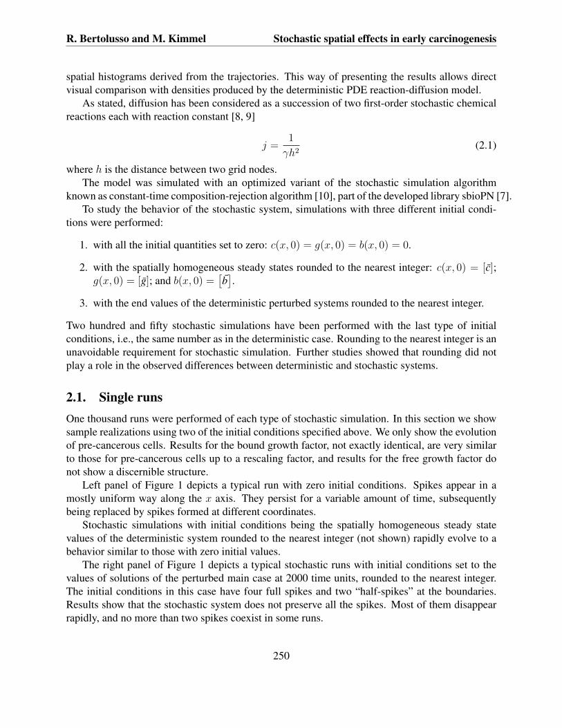
2.1. Single runsOne thousand runs were performed of each type of stochastic simulation. In this section we showsample realizations using two of the initial conditions specified above. We only show the evolutionof pre-cancerous cells. Results for the bound growth factor, not exactly identical, are very similarto those for pre-cancerous cells up to a rescaling factor, and results for the free growth factor donot show a discernible structure.

Left panel of Figure 1 depicts a typical run with zero initial conditions. Spikes appear in amostly uniform way along the x axis. They persist for a variable amount of time, subsequentlybeing replaced by spikes formed at different coordinates.

Stochastic simulations with initial conditions being the spatially homogeneous steady statevalues of the deterministic system rounded to the nearest integer (not shown) rapidly evolve to abehavior similar to those with zero initial values.

The right panel of Figure 1 depicts a typical stochastic runs with initial conditions set to thevalues of solutions of the perturbed main case at 2000 time units, rounded to the nearest integer.The initial conditions in this case have four full spikes and two “half-spikes” at the boundaries.Results show that the stochastic system does not preserve all the spikes. Most of them disappearrapidly, and no more than two spikes coexist in some runs.

250

R. Bertolusso and M. Kimmel Stochastic spatial effects in early carcinogenesis

x

freq

t

x

freq

t

Figure 1: Single runs of the stochastic reaction-diffusion system. Left panel depicts a run with zeroinitial conditions, while the right panel depicts a run with initial condition set to the end values ofthe deterministic system rounded to nearest integer. In both cases, γ = 100.

2.2. Averages of 1000 runsFigure 2 shows a comparison between deterministic (unperturbed) and stochastic systems. Theaverage of the number of pre-cancerous cells in the stochastic simulation using zero initial condi-tions is significantly lower than the result of the deterministic simulation (5.86 compared to valuesbelow 1). This behavior is also paralleled by the bound growth factor (not shown). As for thefree growth factor, for both types of initial conditions, it seems to converge to values close to thedeterministic one.

To further analyze the cause of this behavior, we performed deterministic and stochastic sim-ulations for the associated reaction-only model, and we present the results in the right column ofFigure 2. The deterministic and stochastic mean values of the density of pre-cancerous cells differalmost six-fold, in a way similar to what is observed in the spatial case. The deterministic meanvalues for free growth factor are identical for spatial and non-spatial cases.

However, the stochastic mean of the free growth factor differs with respect to the non-spatialstochastic mean, both in initial shape and in the equilibrium values achieved. The first rapidlyincreases and decreases at the initial time units, reaching a stable plateau at about 0.4 at time 500.The second, in contrast, rapidly grows until reaching a plateau at about 0.7 in a very short time.

The initial increase and decrease in mean values for the spatial case may be related to thediffusive characteristic of free growth factor: as it is not produced equally along the x axis, theobserved effect may be related to an initial imbalance that is compensated as time progresses.However, this is speculative and it does not explain why the reaction-diffusion and reaction-onlysystems achieve a different equilibrium level.

Figure 3 shows a comparison of the perturbed deterministic main case system and the averagesof 1000 runs of the stochastic system, assuming as initial conditions the values of the deterministicsystem at time 2000 rounded to the nearest integer. The initial-value spikes of the pre-cancerouscells rapidly fall to about two thirds of the initial value, and then continue to decrease at a lowerrate. Based on this alone, it is not clear if after 2000 time units the spike values continue to

251

R. Bertolusso and M. Kimmel Stochastic spatial effects in early carcinogenesis

0 500 1000 1500 2000

01

23

45

6

c

C

5.861.41

0 500 1000 1500 2000

0.0

0.5

1.0

1.5

2.0

2.5

3.0

g

G

0.470.72

x

dens

t

x

freq

t

dens

freq

t

x

dens

t

x

freq

t

dens

freq

t

Figure 2: Comparisons of the deterministic and stochastic reaction-diffusion and reaction-onlysystems. Zero initial conditions are assumed. Depicted are, in the first row, pre-cancerous cellsand, in the second row, free growth factor. First column shows deterministic averages, while thesecond column shows averages of 1000 stochastic runs. Third column shows the reaction-onlysystem (blue lines: deterministic solutions, red lines: averages ± 3 standard errors of of 1000stochastic runs). Insets depict values at time 2000.

252

R. Bertolusso and M. Kimmel Stochastic spatial effects in early carcinogenesis

x

dens

t

x

freq

t

x

freq

t

x

dens

t

x

freq

t

x

freq

t

Figure 3: Deterministic versus stochastic reaction-diffusion systems comparison, after perturba-tion. First row depicts the density of pre-cancerous cells; second row depicts the number of freegrowth factor molecules. First column: deterministic evolution after perturbation. Second andthird columns: averages and standard deviations, respectively, of 1000 stochastic runs with initialconditions set to the values of the deterministic system at time 2000 rounded to the nearest integer.

253

R. Bertolusso and M. Kimmel Stochastic spatial effects in early carcinogenesis

decrease until they reach a limit value or until reaching the same level as in Figure 2. Vanishing ofthe “half-spikes” at the boundaries suggests the second option.

x

dens

t

x

freq

t

x

freq

t

x

dens

t

x

freq

t

x

freq

t

Figure 4: Deterministic versus stochastic system comparison for different values of parameter γ.First column depicts evolution of perturbed deterministic systems. Second column depicts averagesof 1000 stochastic runs. Third column depicts single stochastic runs. The stochastic simulationshave initial condition set to the values at time 2000 of the deterministic system rounded to thenearest integer. All cases: n = 3. First row: γ = 1; second row: γ = 10.

To address this issue a new series of 1000 runs was performed for the main case with timeranging up to 8000 units. The results (not shown) exhibit that, in the long run, the averaged spikesdisappear from the stochastic system.

3. Behavior of the system for different rates of diffusionLet us remind that in the so-called main case, the parameter values assumed were n = 5 and γ =100. In this section we will present a comparison of deterministic and stochastic results obtainedwhen studying the case n = 3 for the range of γ values that we studied: γ = 1; 10; 100; 1000; and

254

R. Bertolusso and M. Kimmel Stochastic spatial effects in early carcinogenesis

10, 000. As γ is the reciprocal of the diffusion constant, lower values of γ are equivalent to higherdiffusion rates, given equal scaling.

x

dens

t

x

freq

t

x

freq

t

x

dens

t

x

freq

t

x

freq

t

Figure 5: Further deterministic versus stochastic system comparison for different values of param-eter γ. First column depicts evolution of perturbed deterministic systems. Second column depictsaverages of 1000 stochastic runs. Third column depicts single stochastic runs. The stochastic sim-ulations have initial condition set to the values at time 2000 of the deterministic system rounded tothe nearest integer. All cases: n = 3. First row: γ = 100; second row: γ = 1000.

We have chosen n = 3 because the resulting deterministic systems exhibit two full and two“half-spikes” for γ assuming values 1 and 10, providing good initial values for the stochasticsimulations. Deterministic systems with other n values provide less interesting initial values forthese γ values (most of them only show the “half-spikes” at the boundaries for at least one of the γvalues, as it happens in the main case). Other parameter combinations are not shown because theylead to the same conclusions as the case n = 3.

The results, presented in Figures 4 and 5 for increasing values of γ, are organized as follows:each figure shows results for two different values of γ, one in the first row and the other in thesecond row. Left column shows the deterministic simulations of the perturbed system. Middle col-umn shows the average of 1000 stochastic runs. Right column shows one representative stochasticrun.

255

R. Bertolusso and M. Kimmel Stochastic spatial effects in early carcinogenesis

Based on the computations, the stochastic system better preserves the averaged spikes of thepre-cancerous cells and the bound growth factor (not shown), if lower values of γ are assumed, or,equivalently, if diffusion is higher. It even seems the average spike height is indefinitely preservedin time for γ = 1 (first row of Figure 4). Single runs show that one of the original spikes is main-tained through completion of simulation, while the rest disappear rapidly. By observing the plot ofthe averages, it seems that the internal spikes are preserved with greater probability compared tothe boundary spikes.

5 10 15 20 25

010

2030

4050

Vxl_025−Gm_00100−n_5−eps_0.01−NewmnBC−ect_1e−09

x

Cel

ls

38.37

42.91

36.88 36.88

42.91

38.37

23.42

0 500 750 1000 2000

0 10 20 30 40 50

010

2030

4050

Vxl_050−Gm_00100−n_5−eps_0.01−NewmnBC−ect_1e−09

x

Cel

ls

30.5531.67

29.52 29.5231.67

30.55

11.71

0 500 750 1000 2000

0 20 40 60 80 100

010

2030

4050

Vxl_100−Gm_00100−n_5−eps_0.01−NewmnBC−ect_1e−09

x

Cel

ls

26.26 26.45 25.69 25.69 26.45 26.26

5.86

0 500 750 1000 2000

0 50 100 150 200

010

2030

4050

Vxl_200−Gm_00100−n_5−eps_0.01−NewmnBC−ect_1e−09

x

Cel

ls

23.98 24.01 23.7 23.7 24.01 23.98

2.93

0 500 750 1000 2000

0 100 200 300 400

010

2030

4050

Vxl_400−Gm_00100−n_5−eps_0.01−NewmnBC−ect_1e−09

x

Cel

ls

22.82 22.83 22.68 22.68 22.83 22.82

1.46

0 500 750 1000 2000

x

dens

x x

x

dens

x

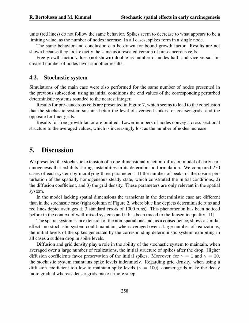
Figure 6: Cross sections of evolution of perturbed deterministic systems for different grid densities.Depicted are densities of the pre-cancerous cells. Horizontal axis shows the number of grid nodesin the interval 0 ≤ x ≤ 1.

In the second row of Figure 4 (γ = 10) a similar behavior can be observed for the internal butnot for the boundary spikes. Single runs show that the boundary spikes disappear rapidly whileone of the internal spikes is maintained throughout the duration of simulations.

First row of Figure 5 depicts the case using γ = 100 that, as expected, shows behavior similarto that observed on the main case for the averaged values (Figure 3): a marked drop from the initialvalues followed by a gradual decay. The same can be said about the similarities found among singleruns compared to the ones of the main system (Figure 1).

The bottom portion of Figure 5 depicts how the deterministic system becomes numericallyunstable for γ = 1000. In contrast, the stochastic system, exhibits the type of behavior observed inFigure 2.

256

R. Bertolusso and M. Kimmel Stochastic spatial effects in early carcinogenesis

Finally, for γ = 10, 000 (not shown) both the deterministic and stochastic systems revert to thespace-homogeneous non trivial equilibrium state.

4. Consequences of varying the grid density

x

freq

t

x

freq

t

x

freq

t

x

freq

t

x

freq

t

Figure 7: Stochastic reaction-diffusion system. Averages of 1000 runs for different grid densities.The numbers of grid nodes appear on the top of each panel.

4.1. Deterministic systemFigure 6 shows cross sections of time evolution of pre-cancerous cells density in the perturbeddeterministic system for different number of nodes: 25, 50, 100, 200, and 400. Orange lines thatlook like horizontal straight lines are the cosinusoidal perturbations of the corresponding spatiallyhomogeneous steady state.

The spatially homogeneous steady states are twice larger in magnitude if the number of nodesare halved, and the opposite holds true if the number of nodes are doubled. Values at 2000 time

257

R. Bertolusso and M. Kimmel Stochastic spatial effects in early carcinogenesis

units (red lines) do not follow the same behavior. Spikes seem to decrease to what appears to be alimiting value, as the number of nodes increase. In all cases, spikes form in a single node.

The same behavior and conclusion can be drawn for bound growth factor. Results are notshown because they look exactly the same as a rescaled version of pre-cancerous cells.

Free growth factor values (not shown) double as number of nodes half, and vice versa. In-creased number of nodes favor smoother results.

4.2. Stochastic systemSimulations of the main case were also performed for the same number of nodes presented inthe previous subsection, using as initial conditions the end values of the corresponding perturbeddeterministic systems rounded to the nearest integer.

Results for pre-cancerous cells are presented in Figure 7, which seems to lead to the conclusionthat the stochastic system sustains better the level of averaged spikes for coarser grids, and theopposite for finer grids.

Results for free growth factor are omitted. Lower numbers of nodes convey a cross-sectionalstructure to the averaged values, which is increasingly lost as the number of nodes increase.

5. DiscussionWe presented the stochastic extension of a one-dimensional reaction-diffusion model of early car-cinogenesis that exhibits Turing instabilities in its deterministic formulation. We compared 250cases of each system by modifying three parameters: 1) the number of peaks of the cosine per-turbation of the spatially homogeneous steady state, which constituted the initial conditions, 2)the diffusion coefficient, and 3) the grid density. These parameters are only relevant in the spatialsystem.

In the model lacking spatial dimensions the transients in the deterministic case are differentthan in the stochastic case (right column of Figure 2, where blue line depicts deterministic runs andred lines depict averages ± 3 standard errors of 1000 runs). This phenomenon has been noticedbefore in the context of well-mixed systems and it has been traced to the Jensen inequality [11].

The spatial system is an extension of the non-spatial one and, as a consequence, shows a similareffect: no stochastic system could maintain, when averaged over a large number of realizations,the initial levels of the spikes generated by the corresponding deterministic system, exhibiting inall cases a sudden drop in spike levels.

Diffusion and grid density play a role in the ability of the stochastic system to maintain, whenaveraged over a large number of realizations, the initial structure of spikes after the drop. Higherdiffusion coefficients favor preservation of the initial spikes. Moreover, for γ = 1 and γ = 10,the stochastic system maintains spike levels indefinitely. Regarding grid density, when using adiffusion coefficient too low to maintain spike levels (γ = 100), coarser grids make the decaymore gradual whereas denser grids make it more steep.

258

R. Bertolusso and M. Kimmel Stochastic spatial effects in early carcinogenesis

Simple versions of the model with µ = 0 and constant positive κ, which lend themselves toa more detailed analysis were studied in ref. [6]. It was shown that in this case regular spatiallyinhomogeneous stationary solutions were unstable. Consequently, the pattern observed in numer-ical simulations might be a dynamical structure with the maxima growing to infinity with time.Moreover, it was determined in ref. [6] that there existed discontinuous inhomogeneous steadystates, which were also unstable. Numerical simulations suggested emergence of distributionalinhomogeneous steady states.

The results of our current research, as presented in this paper, add to this complexity. Fourversions of the carcinogenesis model, resulting from taking or not taking into account the stochasticand spatial effects may exhibit very different dynamics. In particular, the mathematically intriguingbehavior of the deterministic model with spatial effects is partly destroyed when stochastic effectsare also added. What is the relevance of these results for the true biological system? Only refinedexperimental results may help answer this question.

Much of spatial modeling in biology has been accomplished using partial differential equationswithout reference to stochasticity. Almost without exceptions, this style of modeling hinges uponpresumption that continuity provides the glue which allows using the machinery of calculus. In thesystems considered in this paper, the continuity acts to produce asymptotically irregular (spiky)solutions. Stochasticity causes, in the mean, these spikes to gradually dissolve. At the singlerealization level, the stochastic system preserves enough spikeness to be a model of spontaneousformation of early cancer foci. However, they are now frequently reversible (Figure 1), while newones are appearing. The qualitative picture is more complicated as a result.

AcknowledgmentsThe authors thank two anonymous referees for their helpful comments. Also, discussions with Dr.Anna Marciniak-Czochra are gratefully acknowledged. RB was supported by the NIGMS grantGM086885. MK was supported by the Polish NCN grant NN514411936.

References[1] A. Marciniak-Czochra, M. Kimmel. Reaction-difusion model of early carcinogenesis: The

effects of influx of mutated cells. Mathematical Modelling of Natural Phenomena, 3 (2008),No. 7, 90–114.

[2] A. Marciniak-Czochra, M. Kimmel. Dynamics of growth and signaling along linear and sur-face structures in very early tumors. Computational & Mathematical Methods in Medicine,7 (2006), No. 2/3, 189–213.

[3] A. Marciniak-Czochra, M. Kimmel. Modelling of early lung cancer progression: Influence ofgrowth factor production and cooperation between partially transformed cells. Math. Mod.Meth. Appl. Sci., 17S (2007), 1693–1719.

259

R. Bertolusso and M. Kimmel Stochastic spatial effects in early carcinogenesis

[4] A. Marciniak-Czochra, M. Kimmel. Reaction–diffusion approach to modeling of the spreadof early tumors along linear or tubular structures. Journal of Theoretical Biology, 244 (2006),No. 3, 375–387.

[5] A. Marciniak-Czochra, M. Ptashnyk. Derivation of a macroscopic receptor-based model us-ing homogenization techniques. SIAM J. Math. Anal., 40 (2008), No. 1, 215–237.

[6] A. Marciniak-Czochra, G. Karch, K. Suzuki. Unstable patterns in reaction-diffusion modelof early carcinogenesis. arXiv:1104.3592v1, (2011).

[7] R. Bertolusso. Computational models of signaling processes in cells with applications: Influ-ence of stochastic and spatial effects. PhD thesis (2011), Rice University, Houston, TX.

[8] R. Erban, S. J. Chapman, P. Maini. A practical guide to stochastic simulations of reaction-diffusion processes. ArXiv e-prints, (2007), April.

[9] S. A. Isaacson, C. S. Peskin. Incorporating diffusion in complex geometries into stochasticchemical kinetics simulations. SIAM J. Scientific Computing, 28 (2006), No. 1, 47–74.

[10] A. Slepoy, A. P. Thompson, S. J. Plimpton. A constant-time kinetic monte carlo algorithm forsimulation of large biochemical reaction networks. J. Chem. Phys., 128 (2008), May, 205101.

[11] J. Paulsson, O. G. Berg, M. Ehrenberg. Stochastic focusing: fluctuation-enhanced sensitivityof intracellular regulation. Proc. Natl. Acad. Sci. U.S.A., 97 (2000), June, 7148–53.

260