Modeling soil moisture: A Project for Intercomparison of ... · JOURNAL OF GEOPHYSICAL RESEARCH,...

JOURNAL OF GEOPHYSICAL RESEARCH, VOL. 101, NO. D3, PAGES 7227-7250, MARCH 20, 1996

Modeling soil moisture: A Project for Intercomparison of Land Surface Parameterization Schemes Phase 2(b)

Yaping Shao Centre for Advanced Numerical Computation in Engineering and Science, University of New South Wales, Sydney, Australia

Ann Henderson-Sellers

Climatic Impacts Centre, Macquarie University, Sydney, Australia

Abstract. In a,n intensive investigation of soil moisture simulation in land surface schemes, a number of numerical experiments was conducted with 14 representative schemes and the results compared with Hydrological and Atmospheric Pilot Experiment- Modeliz&tion du Bilan Hydrique (HAPEX-MOBILHY) data. The results show that soil moisture simulation in current land surface schemes varies

considerably. After adjustment of land surface parameters, the disagreement in soil moisture for a 1.6-m soil layer remains around 100 mm. Correspondingly, the range of variation in predicted annual cumulative evaporation as well as total runoff plus drainage is around 250 mm (annual precipitation being 856 mm for HAPEX- MOBILHY). The partitioning of surface available energy into sensible and latent heat fluxes is closely coupled to the partition of precipitation into evaporation and runoff plus drainage. Although, on average, the range of variation in net radiation is about 8 W m -2, that of both the laterit and sensible heat fluxes is twice as large. These disagreements are related to different causes but attempts to establish the link between the outcome and the responsible mechanism has ha,d only limited success to date because of the complex interactions embedded in the schemes. This study implies that different schemes achieve different equilibrium states when forced with prescribed a, tmospheric conditions a, nd that the time period to rea,ch these sta, tes differs a. mong schemes; a, nd even when soil moisture is fairly well simulated, the processes (particula. rly evaporation and runoff plus drainage) controlling the simulation differ among schemes and at different times of the year. These results suggest that prescription of land surface scheme physics may have to be a, function of the type of predictions (short-term weather forecasting, mesoscale modeling or climate ensembles) required as well as the underlying scheme [ormulation and that scheme simulations must be vMida.ted for all components of the prediction.

1. Introduction: PILPS and Soil

Moisture Simulation

Budyko [1956] proposed a simple land surface scheme for parameterizing the interaction between the atmosphere and the land surface. The parameterization provides the boundary conditions for global climate models. The la.st decade has seen a rapid development of more sophisticated schemes and a rapid expansion in their applications in atmospheric, hydrological, and ecological modeling. However, it is in general not clear how reliable the schemes are and whether the host models

are sensitive to the accuracy of the parameterizations.

Copyright 1996 by the American Geophysical kinion.

Paper number 95JD03275. 0148-0227 [ 96 [95 J D-03275 $05.00

Since 1992, the Project for Intercomparison of Land Surface Parameterization Schemes (PILPS) has been responsible for a number of complementary sensitivity tests [Pitman it et al., 1993] for improved understanding of land surface schemes. The progress and future activities of the project are described in detail by Henderson- Sellers et al. [1995]. The science plan time lines of PILPS are as shown in Figure 1.

Because of the critical importance of soil moisture in atmospheric, hydrological, and ecological models, an intensive investigation of soil moisture simulation in land surface schemes was conducted within the frame-

work of PILPS: the Soil Moisture Simulation Workshop (November 14-25, 1994, Macquarie University, Sydney) comprising PILPS Phase 2(b). The main goals of the workshop included the following: (1) quantification of the differences in soil moisture predictions among land surface schemes, and (2) investigation of whether dif-

7227

7228 SHAO AND HENDERSON-SELLERS: MODELING SOIL MOISTURE

PILPS SCIENCE PLAN TIMELINES

completed 1992 1993 1994 1995 1996 1997 1998 current & proposed

T•sk

Phase 0

(b) Offline (synlh•tic forcing) (Re-PILPS & MINI-PILPS)

(c) Offline (synthe•c forcing) using consistency checks

Plmse 2

Phase 3

Phase 4

Offline (evaluation using obsewed data) (a) Cabauw (deep soil saturated) (b) HAPEX-MOBILHY (Soil moisture) (c) other GClP relevant areas and periods (? BOREAS)

Coupled intercomparisons with host 3-D models (AMIP:12)

Coupled intercomparisons with selected PILPS schemes and hosts

(a) NCAR CCM2 (b) BMRC I.AM (c) GCIP region (with GNEP)

I t

Figure 1. PILPS science plan timelines.

1999

ferences occur because of theory, numerical i•nplemen- tation, coding, or choice of parameters. A number of numerical tests were carried out with 14 representative land surface schemes (Table 1) and the outcomes compared with data from the Hydrological and Atmospheric Pilot Experiment- Modelization du Bilan Hydrique (HAPEX-MOBILHY).

It, is naYve to expect, that such a comparative study should provide detailed explanations for specific features of all schemes, or provide a firin judglnent whether one type of parameterization is superior to others. In- tercomparison is difficult because:

Table 1. Workshop Participants and Land Surface Pa- rameteriza. tion Schemes Studied in the Soil Moisture Workshop

Participants Schemes

Zong Liang Yang BATS Andy Pitman BEST Peter Thornton BGC Alex Haxeltine BIOME2 Parviz Irannejad BUCKET William J. Parton CENTURY Diana Verseghy (?LASS Eva Kowalczyk CSIRO9 Jean-Francois Mahfouf ISBA Joel Noilhan ISBA Dragutin T. Mihailovic LAPS Peter Wetzel PLACE Agnes Ducharne SECHIBA2 Yong Kang Xue SSiB Xu Liang VIC

1. the participating schemes are developed based on different concepts and with different levels of complexity depending on the intended application of the schemes. The schemes can be divided into those for global climate models, Biosphere Atmosphere Transfer Scheme (BATS) [ Dickinson et al., 1992], Bare Essentials of Surface Transfer (BEST) [Pitman et al., 1991], Cana- dian Land Surface Scheme (CLASS) [Vcrseghy, 1991; Vcrseghy ½t al., 1993], CSIRO Soil-Canopy Scheme (CSIRO9) [ Kowalczyk et al., 1991], Schematisation des EChanges Hydriques Interface Biosphere-Atmosphere (SECHIBA2) [Ducoudre et al., 1993], Simplified Simple Biosphere Model (SSiB) [Xue et al., 1991], Variable In- filtration Capacity scheme (VIC) [Liang ½t al., 1994], bucket (BUCKET) scheme [Manabe, 1969]; for mesoscale models, Interaction Soil Biosphere Atmosphere (ISBA) [Noilhan and Planton, 1989], Land Surface Pa- rameterization Scheme (LAPS) [Mihailovic et al., 1993], Parameterization for Land-Atmosphere-Cloud Exchange (PLACE) [Wetzel and Boone, 1995]; and for ecological models, Biogeochemical scheme (BGC) [Running and Hunt, 1993], Biome scheme (BIOME2) [Haxeltine et al., personal communication, 1994], and CENTURY [Par- ton et al., 1993]. Each scheme is intended to capture the important aspects of complicated land surface processes relevant, to the host model. It, is virtually impossible for the individuals responsible for analyzing the results to understand all the details of all schemes.

2. The schemes have a different history in their development. Some schemes are mature and well tested, while others may need further tests and adjustment.

3. More fundamentally, land surface schemes are sys- tems of coupled nonlinear differential equations. The nonlinearity of the schemes makes it very difficult to

SHAO AND HENDERSON-SELLERS' MODELING SOIL MOISTURE 7229

determine the causality between the scheme outcome and the scheme details.

However, the PILPS Phase 2(b) study is important in determining the degree of disagreement among the bulk of participating schemes, identifying the areas where improvements are required and providing stimulating suggestions for possible improvements. Certain behav- ioral aspects of the schemes can be explained to some extent. It must be recognized that this work, as part of PILPS, represents a process for scheme improve- merit. Through their involvement in the process, the scheme developers identify specific problems in their schemes and develop strategies for improvement. A large number of examples demonstrate the importance of this process. These specific problems, such as errors in coding, inadequate parameterization and inadequate scheme structure, are different in nature. Therefore it is inappropriate to discuss these problems in the present paper; instead, they must be addressed separately (e.g., Special Issue of Global and Planetary Change, edited by Henderson-Sellers [1995]).

This paper documents the general results obtained in the Soil Moisture Simulation Workshop. Section 2 sum- marizes the basic differences in theory among schemes, which provides a basis for the design of the experiments and the interpretation of results. In sections 3 and 4, respectively, the HAPEX-MOBILHY data set and the numerical experiments are described. The results are presented in section 5 and the conclusions are in section 6.

2. Theory of Soil Moisture Simulation in Land Surface Schemes

The basis of all schemes tested in this study is the one-dimensional conservation equations for temperature and soil moisture

0o 10G

Ot C Oz

Ow 10Q Ot pw Oz

(1)

where 0 is soil temperature, C is volumetric soil heat capacity, w is volumetric soil water content, pw is the density of liquid water, and Sw is a sink term which includes runoff and transpiration. (The temperature sink term is zero, if there is no phase change in the soil water). The vertical heat flux, G, obeys a simple flux- gradient relationship, and the vertical soil water flux, Q, obeys Darcy's law. A land surface scheme is the algorithm required to solve this system of equations for a particular soil layer configuration. The parameterizations occur in the boundary conditions and in the treatment of the sink terms. The upper boundary conditions at the atmosphere and land surface interfaces include sensible and latent heat fluxes.

It is not helpful to discuss all the detailed differences among a large number of schemes, because it is im-

possible to determine the effect of these differences on the overall performance of the schemes which consist of complicated nonlinear interactions between many components. Nevertheless, the differences in scheme configuration and those in parameterization of individual components are the two major categories of differences worthy of consideration.

2.1. Structural Differences in Soil Moisture Sim- ulation

The structural differences are mainly reflected in the number of soil layers, canopy layers, and the linkage between va. rious components of a scheme. Most schemes use a single layer canopy treated as a "big leaf," except the bucket model which does not have a canopy component. Thus as far as soil moisture simulation is concerned, the major difference in model structure lies in the number of soil layers.

Conceptually, the schemes can be considered as bucket- type single-layer schemes, force-restore-type two-layer schemes and diffusion-type multilayer schemes. Schemes developed for ecological purposes may not fall into these categories.

Single soil layer models. The water balance equation for the active soil layer of depth d (often assumed to be 1 m) is the integrated form of (2)

d dW pw

where W is soil moisture averaged over depth d, Pr is precipitation rate, E is evaporation, R is runoff, and Dr is drainage. Single layer models have two distinct features. First, runoff is commonly assumed zero if soil moisture is smaller than a critical value We, but equals the surface water flux if the soil moisture is larger than Wc. Second, there is a direct feedback between evaporation and soil moisture of the total soil layer, and the hydraulic diffusion process which influences the distribution of water within the soil layer and the availability of soil water for evaporation is ignored. Consequently, rapid fluctuations in evaporation and surface soil moisture cannot be accurately described.

Force-restore models. A two-layer force-restore model has a thin top layer of depth dl and a total soil layer of depth d2. The prognostic equations for soil moisture in the two layers are

0W1 __ Eg - P• W• Ot -- -C1 7• C2 -wg,• (4) OW• _ •+r.,•-m (5) Ot -

where W1 and W2 are soil moistures in the top and the deep soil layer, respectively, and Wg•q is that when gravity balances the capillary force; Eg is evaporation from the bare ground and Etr is the transpiration rate; C1 and C2 are coefficients and r a time constant of 1

day. The force term (-Cl(Zg-Pr)/t9wdl) describes the


rapid response of I/V• to precipitation and evaporation and the restore term (C2W• - 14/]•eq)/r)describes the supply of soil moisture from the deep soil layer which responds slowly to the atmospheric forcing.

In contrast to the bucket model, the force-restore model has two distinctly different time scales in soil moisture simulation and a profoundly different feedback between evaporation and soil moisture. In addition, the force-restore model allows runoff from the surface, the top soil layer and the deep soil layer and the simulation of soil moisture is now coupled with the canopy transpiration process. The force-restore method is used in CSIRO9 and ISBA.

Multilayer diffusion type models. Most multilayer schemes have three layers which give a better resolution of root distribution and better handling of the recharging flow froIll deep soils. The evolution of the depth averaged soil moisture of soil layer i obeys the integrated forIll of (2)

dWi Qi - Qi- 1 dt = p•d• + (6) ,o•

where Sw, is vertically integrated for layer i, which includes the water loss via transpiration and horizontal runoff; the moisture fluxes between the soil layers are determined (in principle) by Darcy's law. Among the schemes tested in the workshop, BATS, BEST, CLASS, LAPS, and SSiB use the diffusion Inethod for moisture in a three-layer soil and PLACE solves the Richards' equation in a five-layer soil. The treatment of the sink term is important, because it not only involves the distribution of roots in soil layers, but also the relationship between canopy transpiration and horizontal runoff.

Other soil moisture schemes. VIC [Liang et at., 1994] uses two soil layers for soil moisture simulation, but the upper layer is designed to represent the dynamic behavior of the soil that responds to rainfall events, and is thicker (0.5 m) than the upper layer in the force- restore models. The lower layer is used to character- ize the seasonal soil moisture behaviour. Roots can be

specified for both layers. Water can flow from the upper layer to the lower layer, but there is no upward moisture flux between the two soil layers.

SECHIBA2 uses a two-layer soil model in which the depth of the layers evolves through tilne. This evolution is driven by the "top-to-bottom" filling (due to precipitation) and drying (due to evapotranspiration) algorithm described by Choisncl [1984]; no explicit diffusion is allowed either between the two layers or at the bottom of the soil, so that it is equivalent to a bucket for runoff and drainage.

In BGC, BIOME2, and CENTURY, water can flow from the upper layer(s) to the lower layer(s) but there is no upward moisture flux within the soil. The water content in each layer is calculated by the water budget of the layer at each time step. The number of layers is two in BIOME2 (similar to VIC), three in BGC (similar to BATS), and up to eight in CENTURY.

2.2. Soil Moisture and Soil Temperature

The treatment of the interaction between soil mois-

ture and soil temperature depends very much on the structure of each scheme. For a bucket model, the vertically integrated conservation equation for soil temperature can be simplified to

c9T R• - H- A E at = (7)

assuming the heat flux at the lower boundary of the soil layer is zero, where R,• is net radiation, H is sensible heat flux, and • is the latent heat of vaporization. Therefore for a bucket model, evaporation is the major pathway for coupling soil moisture and soil temperature.

For schemes with more than one soil layer and explicit treatment of canopy processes, the interaction between soil moisture and soil te•nperature is very complicated. Although evapotranspiration remains the pathway for interaction, it, now involves a canopy water reservoir, transpiration and differences in canopy, and bare soil albedo. It is difficult in general to identify how this interaction will impact on the performance of a scheme, because of the nonlinear relationships involved.

2.3. Differences in Parameterization

Evaporation, transpiration, and runoff plus drainage determine the soil moisture budget and these components are parameterized very differently in the participating schemes.

Evaporation. It, is assumed in all schemes that evaporation is proportional to a scaling evaporation, Ep. One method of calculating the potential evaporation is the aerodynamic resistance formulation

Ep - P(qsat -- qa)/ra (8)

where p is air density, ra is aerodynamic resistance, qsat is saturation specific humidity and qa is the specific humidity of air. BATS, BEST, BUCKET, ISBA, LAPS, CLASS, PLACE, SSiB and SECHIBA2 use the aerodynamic formulation for calculating the potential evaporation. CSIRO9, BGC, VIC and CENTURY use the Penman-Monteith formulation and BIOME2 uses

the Priestley-Taylor formulation. The Priestley-Taylor, the Penman-Monteith, and the aerodyna•nic formulations are not fundamentally different. The Penman- Monteith formulation assumes that the aerodynamic resistance for heat transfer and evaporation is identical and takes into account the effect of advection on evaporation. It reduces to the Priestley-Taylor formulation, if the advective effect is neglected. Ep estimated from the Penman-Monteith formulation is somewhat smaller

than that estimated by using (8) [e.g. Garratt, 1992, chapter 5].

For unsaturated soils, the actual evaporation, Eg, differs from the potential evaporation. Three methods, the c• method, the • method and the threshold method, are

SHAO AND HENDERSON-SELLERS: MODELING SOIL MOISTURE 7231

commonly used for its calculation' described by

p(.qsat(Tg) - qa)lra t• method Eg - /3E v /3 method min. { Ep, Ec } threshold method

where a and /3 are functions of soil moisture. The threshold formulation implies that evaporation proceeds at the potential rate until the soil moisture is sufficiently depleted, then evaporation is determined by the water flux from the soil Ec. The c• and /• formulations have the same physical interpretation as the threshold formulation and can be reduced to the latter if c• and •3 are adequately chosen (e.g., c• = exp(-½-g) with •bg being the soil water potential of the top soil layer, •3 = i for Zp < nd/3 = Z/Zp _< difrernc in evaporation schemes, therefore, lies in the estimation of c•, •3 and Ec.

Among the 14 schemes, BATS, PLACE, and BIOME2 use supply and demand formulation; BEST, BUCKET, CSIR.O9, SECII[BA2, VIC, and CENTURY use the •3 formulation, while ISBA, LAPS, SSiB and CLASS use the a formulation.

Transpiration. Transpiration is a physiological process associated with photosynthetic activities, which involves the transfer of water from soil through the roots, stems, branches, and leaves. The parameterization of transpiration is achieved by introducing a canopy resistance as a measure of the effectiveness of moisture

transfer. For fully vegetated surfaces, transpiration is

Err - p(q. at(Tc)- qa)/(ra + rst) (9)

with rst being the bulk stomatal resistance or bulk canopy resistance.

In most of the schemes, the stomatal resistance of a leaf, Rst, is calculated and the bulk stomatal resistance, rst, is obtained by assuming that

rst- Rst/LAI (10)

where LAI is leaf area index. R,t is modified from a minimum leaf stomatal resistance by considering several constraints. For instance, the expression used in ISBA [Noilhan and Planton, 1989] is

]•st - i•st,minF1f•-l f.•-l f•-I (ll)

where F1, F2, Fa and F4 are, respectively, functions representing the effects of photosynthetically active radiation, soil moisture, vapour pressure deficit of the atmosphere, and air temperature on the stomatal resistance. More functions can be used in the above expression if more constraints are to be applied.

Depending on how the functions are specified, the expression for stomatal resistance can be very different. More importantly, depending upon how this parameterization is implemented in a specific scheme, a

III

IV

Figure 2. Schematic illustration of runoff plus drainage for land surface sche•nes represented in the workshop. According to the number of soil layers, the schemes are classified into group 1 (single-layer models), group 2 (two-layer models), group 3 (three-layer models), and group 4 (multilayer models).


comparison of transpiration becomes extremely difficult [Mahfouf et al. 1995].

Runoff and drainage. Runoff plus drainage is closely connected with the configuration of the soil layers. As illustrated in Figure 2, the schemes tested in this study can be divided into four groups. SECHIBA2 and the bucket, model are the one-layer models with only one drainage process and a pseudosurface runoff; BEST, BIOME2, CSiRO9, ISBA, and VIC are two- layer models with flow out from the sides and/or the base; BGC, BATS, CLASS, LAPS, and SSiB are three- layer models with disparate boundary conditions; and CENTURY and PLACE have tnore than three layers, also with disparate boundary conditions. Some schemes with two or more layers explicitly include moisture diffusion between soil layers, while others (BGC, BIOME2, CENTURY, and VIC) do not permit upward diffusion.

In terms of the drainage and subsurface flow formulations, the 14 models can be classified into two major types: those keyed to values of intermediate soil moisture (field capacity and/or wilting point) and those which apply a (continuous) nonlinear function relat- ing soil moisture to key diffusive parameters such as hydraulic conductivity and water potential [Wetzel et al., 1995]. While most schemes key their drainage to field capacity, PLACE and VIC allow the soil to drain without limit, with an asymptotic approach to zero soil moisture during a very long dry period. The nonlinear soil water functions vary widely from model to model, including empirical relationships derived from large- scale catchment hydrology, soil column studies, labo- ratory work, and theory.

3. The HAPEX-MOBILHY Data Set

and Surface Parameters

3.1. The Data Set

The HAPEX-MOBILHY data set, which forms the basis of the verification, is chosen for the following three reasons:

1. A data set needs to offer long periods (years) of high-resolution measurements of atmospheric fluxes, atmospheric forcing, soil moisture, hydrological fluxes, biomass accumulation and surface properties (soil type, vegetation, and surface aerodynamic properties). The HAPEX-MOBILHY data set is reasonably complete and is of relatively high quality.

2. The HAPEX-MOBILHY data set can be used by all schemes without great numerical difficulties.

3. Two of the workshop participants (J. Noilhan J.- F. Mahfouf) have many years of experience with the data set and detailed understanding of its accuracy and reliability.

The HAPEX-MOBILHY data set consists of weekly soil moisture measurements down to 1.6 m at 0.1-m

intervals and energy flux measurements during the In- tensive Observation Period (May 28 to July 3, 1986)

together with a full year's atmospheric forcing measurements, including downward shortwave radiation, downward infrared radiation, precipitation, air temperature, wind speed, surface pressure, and specific humidity. De- tails of the data set are given in a series of publica- tions documenting the HAPEX-MOBILHY experiment [e.g., Goutorbe et al., 1989; Goutorbe and Tarrieu, 1991; Goutorbe, 1991].

The HAPEX-MOBILHY data used in this study have been prepared by J.-F. Mahfouf and J. Noilhan, and have been used on several occasions for calibration

of ISBA by, for instance, Mahfouf[1990] and Jacquemin and Noilhan [1990].

The data were obtained from HAPEX-MOBILHY at

Caumont (SAMER 3, 43041 ' N, 006 ' W, mean altitude 113 m). Detailed information on the SAMER network and the site can be found in work by Goutorbe [1991]. Most of the forcing data were taken from Caumont, particularly during the Intensive Observation Period. If data at Caumont were missing, measurements from neighbouring meteorological stations were used. There- fore the forcing data may not be fully consistent with the validation measurements for short and inter-mittent

time periods. However, this inconsistency in the data should not have a significant effect on the intercomparison and validation of land surface schemes.

The chosen location is a soya crop field. Soya plants start to grow in May and are harvested at the end of September. Although HAPEX-MOBILHY was conducted in a heterogeneous area, the immediate sur- roundings of Caumont can bc considered as uniform on a scale of several hundred metres. For the HAPEX-

MOBILHY area at large, surface fluxes reveal the sig- nature of the two main ecotypes: coniferous forest and crops (SAMEPt. 3 represents one of the crops). Analysis of soil moisture also splits soil texture into two broad categories: sand and loam. The soil type at Caumont is loam. The parameters used for characterizing the land surface are summarized in the instructions for experiment 1 (see appendix).

For schemes with two or more layers, a quantitative description of root distribution is necessary. HAPEX- MOBILHY data do not include observations of roots.

Thus the quantification of root distribution cannot be based on measurements but on the experience that soya plant has its root system concentrated in the first 0.5 m of soil. The crop height and zero displacement height are also empirically derived, but land surface schemes are insensitive to these two parameters. Albedo is based on radiative measurements which revealed a nearly constant value of 0.2 during the year.

The measurements of soil moisture were made using neutron sounding probes, every week at every 0.1 m from the surface down to 1.6 m. Details of soil moisture

measurements using neutron probes, including theory, sensor calibration, and data manipulation are as described by Cuenca and Noilhan [1991].

Various terms of the surface energy balance recorded


350

• 250-

• •5o-

= 100-

50-

o 14o

lOP = day 148 to day 182

3.72 mm/day .." (from flux measurements) .."

2.99 ram/day (from water budget:

ß assumes no runoff)

LH flux

P - dSW

150 160 1'•0 1 •0 1•0 2t•0 210 2•0 2•0 240 Yearday

Figure 3. Cumulative evaporation (millimeters) during the intensive observation period at the Caumont site, estimated from observed latent heat fluxes and estimated from soil moisture with the assumption of zero runoff plus drainage.

by the SAMER. station every 15 min are available for the Intensive Observation Period at Caumont. Net ra-

diation, ground heat flux, and sensible heat fluxes are directly measured, while the latent heat flux is the resid- ual term required to close the surface energy budget. According to the assessment of Goutorb½ [1991], the accuracy of the flux measurements is possibly around 15% at short time scales and around 10% at longer timescales (for instance, monthly).

The data set is not. fully self-consistent, in particular between soil moisture and evaporation measurements. From the water budget equation, the cumulative evaporation can be expressed as

Ed! - P•d! - dm (12) o

if runoff plus drainage is negligible {which is possibly true for the Intensive Observation Period), where E is evaporation, P• is precipitation and m is the total amount of water in the soil layer. Figure 3 compares the cumulative evaporation estimated from the above equation with that estimated from the latent heat fluxes.

The inconsistency amounts to 25 mm for the intensive observation period.

3.2. The Parameters

The parameters used in this work are given in the appendix and it suffices here to make two comments. Monthly mean leaf area index (LAI), fractional vegetation cover (FVEG), overall surface roughness length (z0), canopy roughness length (z0•), zero displacement height (z•), and the height of canopy (h•), are as speci-

fled in the appendix. These quantities are interpolated to smaller time intervals when required (see section 4).

The roots of soya plants were assumed to be shallow and are distributed mainly in the top 0.5 m. The year was divided into the bare soil period (January to April, October to December), the transition period (May) and the growing season (June to September). For the bare soil period, there were no roots; for the transition period, it was assumed that the top 0.1-m soil layer contains 70% of the roots and the soil layer between 0.1 to 0.5 m contains the rest, that is, 30%; for the growing season, 00, 30 and 10% roots were assumed to be in the soil layers 0-0.1 m, 0.1-0.5 m, and 0.5-1.0 m, respectively.

4. Numerical Experiments

Fifteen numerical experiments conducted for the workshop are listed in Table 2. The details about the design, purpose, and rationale of these experiments are reported by $hao et ai. [1995]. A land surface scheme is understood as conaprising three basic components for the treatment of bare soil transfer processes, canopy transfer processes, and soil thermal and hydraulic processes. A control experiment was conducted, followed by three other types of experiments: bare soil evaporation tests (experiments 2al and 2a2), sensitivity test for drainage (experiment 2c, 2el) and transpiration test (experiment 3), in an attempt to compare the three basic components of land surface schemes. For the purpose of this study, it, is sufficient for us only to describe the control experiments, experiment 2c and 2el in some detail.


Table 2. List of Numerical Experiments Conducted for the Soil Moisture Workshop

Experiment Description

1

24

2b

3

4

5

11

12

13

14

15

241

2a2

2c

2cl

31

Preworkshop Experiments Control experiment with preworkshop version of schemes Comparison of bare soil evaporation formulations Comparison of evaporation and top layer soil moisture feedback Comparison of transpiration formulations Comparison of soil hydraulic treatment for bare soil Comparison of soil hydraulic treatment for vegetated soil

During-workshop Experiments Control experiment with surface aerodynamic parameters

specified for every time step Control experiment with wilting soil moisture set as the minimum

soil moisture measured in top 0.5-m soil layer Control experiment with a new set of soil hydrological

parameters Sensitivity test for leaf area. index Control experiment with updated version of schemes Comparison of bare soil evaporation formulations in

updated schemes Comparison of bare soil evaporation with specified

drag coefficient Sensitivity test for drainage parameterization Sensitivity test for drainage parameterization Comparison of evapotranspiration formulations in

updated schemes Sensitivity test for transpiration

4.1. Control Experiments (Expe, riments 1, 11, 12, and 13)

Among these experiments, experiment 1 is the pilot control experiment, while experiments ll, 12, and 13 are the improved ones conducted after a preliminary analysis of experiment 1. The purposes of the control experiment are to quantify the differences among the schemes, to verify the simulations against observations and to provide a reference for the other experiments conducted as part of the workshop.

Experiment 1 was first compared with the HAPEX- MOBILHY data and it was found that the disagreement between the simulations and the observations can be re-

duced if more strictly specified parameters for the land surface are chosen (see section 6). experiments 11, 12, and 13 were carried out for this purpose.

Experiment 11. In experiment 1, the aerodynamic properties of the surface were specified by the monthly averages of leaf area index, aerodynamic roughness length, zero-displacement height, and fractional vegetation cover. The low resolution of the aerodynamic parameters (specified for every month) is in- consistent with the high resolution of the atmospheric forcing data (specified every 30 rain). Several schemes, especially those for ecological models, were found sensitive to the resolution of leaf area index.

In experiment 11, the above aerodynamic parameters are specified for every time step under the assumption that LAI and vegetation height increase linearly in the first two months of the growing season with the maximum LAI being 4 and vegetation height being im. The fractional vegetation cover (f•,•a) is derived from LAI using the relationship,

f,,•g = 1 - c -•z'At (13) where the coefficient c is set to 0.6 which is appropriate for soya crops. The aerodynamic roughness length and zero displacement height are derived from LAI and h from the empirical relationships suggested by Raupach [1994].

Experiment 12. For several schemes, the choice of wilting point, Wwitt, strongly influences soil moisture prediction. In experiment l, Wwitt is assumed to be 0.2 m3/m 3 which corresponds to the observed minimum soil moisture averaged over the total 1.6 m soil layer. However, the observed mini•num soil moisture averaged over the top 0.5-m soil layer, which is assumed to contain most of the roots (90% is assumed in the experiments), was less than 0.2 m'3/m :3. Experiment 12 is the same as experiment 11, except that Wwilt is assumed to be 0.12 m3/m • corresponding to the observed minimum soil moisture in the top 0.5-m soil layer.

Experiment 13 and 14. Since soil moisture in the


top soil layers may be influenced by evaporation, it was estimated based on work by Cosby et al. [1984] that the most appropriate value for I4/•,itt for the HAPEX- MOBILHY experiment site is 0.15 m3/m 3. On the basis of the soil texture, taken at the Caumont site (sand, 37 %; silt, 46 %; clay, 17 %), the multiple linear regression analyses described by Cosby et al. [1984] were used to determine soil water potential, saturation soil water potential and saturation soil hydraulic conductivity. The soil hydraulic parameters used for experiment 13 are as specified in the appendix. Experiment, 14 is as experiment 13 but with halved leaf area index.

4.2. Sensitivity Test for Drainage (Experiment 2c, 2cl)

Soil moisture is determined by precipitation, evaporation, and drainage. The different treatments of drainage in land surface schemes may lead to profound differences in soil moisture. Experiments 2c and 2el are drainage sensitivity tests in which the amount of drainage and the residence time of water in the soil layers are investigated. Experiments 2c and 2cl are performed for the HAPEX-MOBILHY bare soil period (first 120 days) with the surface and soil parameters as specified for experiment 13. Evaporation was assumed to be zero, and precipitation was assumed to be 5 and l0 times that of the observed values for experiment 2c and 2cl, respectively. Detailed results from these experiments are reported by Wctz½l et al. [1995].

5. Results

In this section, a quantitative assessment of soil moisture simulation by the participating schemes is provided. The importance of this work lies in the investiga-

tion of the disagreement, and thus the assessment of the capability of land surface schemes for soil moisture simulation. Several general problems are discussed, such as the energy and soil moisture budget, scheme equilibration and scheme sensitivity to the choice of parameters. The details of individual schemes are not reviewed, since they are discussed in detail in a series of papers to be published elsewhere. Most of the conclusions are based on experiment 13 (Table 2), the final control experiment of the workshop, since the results of experiment 2al, 2a2, 2c, 2el and 3 have been discussed by Mahfouf et al. [1995], Wetzel et al. [1995] alld Desborough et al. [1995]. The results from LAPS are excluded from discussion because of numerical difficulties, but have been adequately discussed by Mihailovic and Rajkovic [1995].

5.1. Different Schemes, Different Predictions

The results show that the different, schemes produced profoundly different predictions of soil moisture. The predicted total soil moisture for the 1.6-m soil layer from experiment 13 is compared with the HAPEX- MOBILHY measuredneAts in Figure 4, with -l-10% error margins. (The error margins are indicative, but according to previous studies [e.g., Mahfouf, 1990; Cuenca and Noihlan, 1991] the -l-10% error margins for the soil moisture measurements are not unreasonable). In comparison with the HAPEX-MOBILHY measurements, all schemes correctly describe the annual cycle of soil moisture variation in a qualitative sense: because of frequent rainfall and low evaporation, the soil remains wet for the first four months of the year with the soil moisture close to the field capacity; as precipitation decreases and the available energy for evaporation increases, the soil water decreases at the beginning of the growing season (early May) and the soil is driest between August

700

600

500

400

300

200

$- .... ß BATS

m- .... ß BIOME2

ß - .... ß BGC

•- .... A CENTURY

,• .... ß ISBA

ß '- .... V CSIRO9

•- .... •> PLACE

• .... + SSiB

-g-----• BUCKET • .... O VIC

•- .... [] BEST

O. .... (> SECHIBA2

• .... <• CLASS

•. --• HAPEX

0 60 120 180 240 300 360

Time (Day) Figure 4. Daily averages of total soil water (millimeters} in the top 1.6 m from experiment 13 simulated by different schemes and in comparison with HAPEX-MOBILHY data {weekly measurements}. Shaded area represents the HAPEX-MOBILHY data with -+-10% error margin.


220

120

' I ' I ' I ' I ' I ' •. • HAPEX • .... ß BATS

ß ..... ß BIOME2

•----• BGC

A- .... A CENTURY

•- .... .• ISBA

V- .... V CSIRO9 •- .... •> PLACE

•----F SSiB

•-----• BUCKET (•---E) VlC [•----•] BEST

•---•SECHIBA2 •J---<JCLASS

20 0 60 120 180 240 300 360

Time (Day)

Figure 5. Daily averages of total soil water (millimeters) in the root zone (top 0.5 m) from experiment 13 simulated by different schemes and in comparison with HAPEX-MOBILItY data (weekly measurements). Shaded area represents the HAPEX-MOBILHY data with -4-10% error margin.

and October; and after October the soil becomes in- creasingly wet. However, Figure 4 reveals a significant quantitative disagreement among schemcs and with observations. Soil moisture predictions from five schemes (BATS, BIOME2, BGC, ISBA, and VIC) are in the best agreement, with observations for most times of the year. For the bare soil seasons, the disagreement between the schemes is approximately 70 ram, while dur-

ing the growing season, the disagreement between the schemes is approximately 100 min. Compared with HAPEX-MOBILHY observations, most schemes under- predict soil moisture for most times of year, especially for the growing season.

The comparison of soil moisture in the root zone is illustrated in Figure 5. Again, there is broad agreement between predictions and observations. One out-

-200

-100

I

100

• O'

-100

-200

00 ! ! ! i i 600 400

-200

148 152 156 160 164 168

BATS

ß ...... * HAPEX

Time (Days) Figure 6. Comparison of components of surface energy budget predicted by BATS from experiment 13 and HAPEX-MOBILHY observations, for the first 20 days of the intensive observation period.


600 •

o

-200 'l , I , I -200 0 200 400

SH(HAPEX, W/m2)

600 800

600

400

0

-200 0 200 400 600 800

LH(HAPEX, W/m2)

o

-200- ' • ' • ' -200 -200 0 200 400 600 800 -200 -100 0 100 200

R(HAPEX, W/m2) G(HAPEX, W/m2)

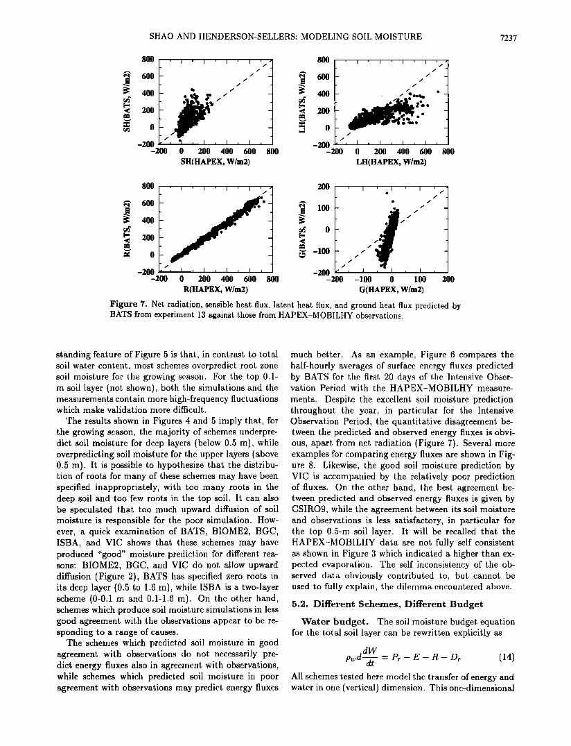
Figure 7. Ne[ radialion, sensible heal flux, la[en[ heal flux, and ground heat flux predicted by BATS from experimen[ 13 agains[ [hose from HAPEX-MOBILHY observations.

standing feature of Figure 5 is that, in contrast to total soil water content, most schemes overpredict root zone soil moisture for the growing season. For the top 0.1- m soil layer (not shown), both the simulations and the measurements contain more high-frequency fluctuations which make validation more difficult.

The results shown in Figures 4 and 5 imply that, for the growing season, the majority of schemes underpre- dict soil moisture for deep layers (below 0.5 m), while overpredicting soil moisture for the upper layers (above 0.5 m). It is possible to hypothesize that the distribution of roots for many of these schemes may have been specified inappropriately, with too many roots in the deep soil and too few roots in the top soil. It can also be speculated that too much upward diffusion of soil moisture is responsible for the poor simulation. How- ever, a quick examination of BATS, BIOME2, BGC, ISBA, and VIC shows that these schemes may have produced "good" moisture prediction for different reasons: BIOME2, BGC, and VIC do not allow upward diffusion (Figure 2), BATS has specified zero roots in its deep layer (0.5 to 1.6 m), while ISBA is a two-layer scheme (0-0.1 m and 0.1-1.6 m). On the other hand, schemes which produce soil moisture simulations in less good agreement with the observations appear to be responding to a range of causes.

The schemes which predicted soil moisture in good agreement with observations do not necessarily predict energy fluxes also in agreement with observations, while schemes which predicted soil moisture in poor agreement with observations may predict, energy fluxes

much better. As an exanlple, Figure 6 compares the half-hourly averages of surface energy fluxes predicted by BATS for the first 20 days of the Intensive Obser- vation Period with the HAPEX-MOBILHY measure-

ments. Despite the excellent soil moisture prediction throughout the year, in particular for the Intensive Observation Period, the quantitative disagreement between the predicted and observed energy fluxes is obvi- ous, apart from net radiation (Figure 7). Several more examples for comparing energy fluxes are shown in Fig- ure 8. Likewise, the good soil moisture prediction by VIC is accompanied by the relatively poor prediction of fluxes. On the other hand, the best agreement between predicted and observed energy fluxes is given by CSIRO9, while the agreement between its soil moisture and observations is less satisfactory, in particular for the top 0.5-m soil layer. It will be recalled that the HAPEX-MOBILHY da.ta are not fully self consistent as shown in Figure 3 which indicated a higher than expected evaporation. The self inconsistency of the observed data. obviously contributed to, but cannot be used to fully explain, the dilemma encountered above.

5.2. Different Schemes, Different Budget

Water budget. The soil moisture budget equation for the total soil layer can be rewritten explicitly as

d dW Pw -•- - P,• - E- R- D,. (14) All schemes tested here model the transfer of energy and water in one (vertical) dimension. This one-dimensional

7238 SttAO AND HENDERSON-SELLERS- MODELING SOIL MOISTURE

, • 800 800 , • , • , • , • •_ • •' 600 600 •

400 / 400

zoo- zoo o o

-200; •' '?' ' • ' • , • , -• -2• 800 0 200 400 600

SH(HAPEX, W/m2)

' I ' I ' I ' I

ß e."•i • e ß

/, I , I , I , I , -200 0 200 400 600 800

LH(HAPEX, W/m2)

800 . , . [ . , . , • 800 . , . ] . , . , .•.

/ ß ee•e ß

o o

-2• /' I , I , I , I -2•- /' ] ' I , [ , [ -2• 0 200 4• 600 8• -• 0 200 400 • 800

SH(HAPEX, W/m2) LH(HAPEX, W/•)

800 , , 800

400-

200

0 -

-200 ' -200

e•le eee . -

] i

I , I , I , I

0 200 400 600 800

SH(HAPEX, W/m2)

600 400

200

0

-200" -200

/ / ,

...

I , I , I 200 400 600 SO0

LH(HAPEX, W/m2)

800

600

400

200

0

[ I /

-200 ß ' I , I , I , I , -200 0 200 400 600 800

SH(HAPEX, W/m2)

800 , , , , , , , , ,•

o -200 - '/' I , I , I , I ,

-200 0 200 400 600 800

LH(HAPEX, W/m2)

Figure 8. Sensible and latent heat fluxes predicted by CLASS, CSIOR9, SSiB, and VIC from experiment 13 plotted agains HAPEX-MOBILHY observations.

assumption is valid if soil properties in the horizon- re(t)- m(0)= •P•(t)- !E(t)- •Ft(t)- IOn(t) (15) tal direction are reasonably homogeneous. Although the one-dimensional assumption, strictly speaking, re- where IPr(t) - fj Prdt is the time integral of Pr and quires that runoff (divergence of horizontal water flux) 'IE, IR and IDr are the integrals of E, R and Dr, re- becomes zero, all schetnes employ an ad hoc runoff term spectively. Since the simulated results are for the equi- for soil moisture adjustment. librium year, we have

An integration of the water budget, equation from time t = 0 to t gives IE + (IR + IDr) = IPr (16)


250

-250

ß .... ß BATS

ß .... ß BIOME2

ß .... ß BGC (NA) A- .... -A CENTURY

ß .... ßISBA ß '- .... -•' CSIRO9

D .... [• PLACE q- .... q- SSiB

-• .... -• BUCKET o .... QvIC E} .... E] BEST

<•> .... •>SECHIBA2 <1 .... <]CLASS

0 60 120 180 240 300 360

Time (Day)

Figure 9. Comparison of running integration of water budget from experiment 13 for partici- paring schemes.

if the integration is performed for 1 year. Figure 9 shows that most schedules conserve water

well. rFhe variation of soil moisture with time is con-

sistent with the soil moisture curves shown in Figures 4 and 5: there is an increase in soil moisture for the

first 4 months, a depletion of soil moisture during the growing season, and an increase in soil moisture in the later part of the year.

However, more detailed analysis reveals that, although land surface schemes can simulate reasonably well at least the annual cycle of soil moisture variation, the

soil moisture budget is achieved in very different, ways. More precisely, the partitioning of precipitation into evaporation and runoff plus drai•age is very different in different schemes. Some schemes achieve soil mois-

ture simulation through large evaporative fluxes, while others have large runoff and drainage coinportents.

The cumulative precipitation for ttAPEX-MOBILHY is shown in Figure 10 (the annual total is 856 mm). Fig- ure 11 shows the integration of total runoff (including surface and subsurface runoff) and drainage from the bottom of the soil layer with time, namely (IR + IDr).

looo I , , , , , , , , , , , t O---OBATS ß .... ß BIOME2

•---•BGC t A-----A CENTURY

4---•ISBA •----•'CSlRO9 D---{•>PLACE +---+ssm 9•-----){(-BUCKET

500 O---¸vIc

•- E}----IE] BEST f' <•>---•SECHIBA2

ß ß <•----<• CLASS

• --- Precipitation

0 0 60 120 180 240 300 360

Time (Day)

Figure 10. Running integration of evaporation from experiment 13. Daily averages are obtained from the time series and then integrated with time. Evaporation (millimeters) is converted from latent heat fluxes (Watts per square meter) with the latent heat of vaporisation being assumed to be 2453 000 J/kg. Integrated precipitation (millimeters) from HAPEX-MOBILHY data is also shown.

7240 SHAO AND HENDERSON-SELLERS' MODELING SOIL MOISTURE

400 , • ,

300

2OO

100

0 60

i

120 180 240 300

Time (Day)

. ,t 360

•- OBATS •-- -• BIOME2

O- -O BGC •r- -• CENTURY •-- 4ISBA • • csmo9 • •PLACE • •ssm • •BUCK•T • •VlC

• •B•ST

• •S•CmBA• • •CLASS

Figure 11. As Figure 10, but for integration of total runoff plus drainage (millimeters).

Figure 11 reveals a significantly different treatment of tive dispersion of the schemes. This result implies that runoff plus drainage among the participating schemes. The total runoff and drainage difference among the models is as large as 200 mm for the year, varying froin 100 to 300 min. BGC, VIC, SECHIBA2, and BIOME2 predict the largest amount of runoff among all schemes, while BEST predicts the smallest. The 200-mm dispar- ity occurred foremost in the first 4 months of the year and after this there is almost no change in the rela-

the parameterizations used by different schemes are extremely different, when the soil is wet.

A similar technique is applied to determine the annual evaporation as shown in Figure 10. Figure 10 shows a significant disagreement in the modeling of evapotranspiration which amounts also to about 200 min. This result is consistent with Figure 11. Schemes with high runoff plus drainage (BGC, VIC, and BIOME2)

350 i , i ' i , i , i ,

300

250

g• 200 .5

+ 150

100

5O

BGC

ß

VlC ß

SECHIBA ß BIOM

ß P-M estimated ß

SSkB

ß

CLASS ß BATS

ß

BUCKET ß PLACE

ß CENTURY

00 550 600 650 700 750 Evaporation (ram)

csmo• BEST

800

Figure 12. Comparison of annual total runoff plus drainage against evaporation (millimeters) for different schemes from experiment 13.

SHAO AND HENDERSON-SELLERS. MODELING SOIL MOISTURE 7241

ß .... 1 BIOME2

• A- .... A CENTURY •---. ISBA

• 80 x7----Vcsmo9 •. •---•.PLACE •.• -+-----]-SSiB = 60 •----•-BUCKET • O---•)VIC

•. •----[z] BEST • &---•>SECHIBA ß -• 40 <t---'<•CLASS ..•

2O

0 0 60 120 180 240 300 360

Time (Day)

Figure 13. Comparison of running integration of net radiation (Watts per square meter) from experiment 13.

have the smallest amount of evaporation, while those schemes with slnall runoff and drainage (CSIRO9 and BEST) have the highest evaporation.

The partitioning of total precipitation into total eva& otranspiration and total runoff plus drainage is shown in Figure 12 where IE is plotted against IR + IDr. As can be seen from (16), all models should fall on a single line with a -1 slope and an intercept equal to the prescribed total precipitation, if they have the correct water budget. All schemes should map onto a single point if they have the same water partitioning. Figure 12 shows clearly that differences in water partitioning between models is extremely large.

Surface Energy Budget. Another partitioning in land surface schemes is that of the surface available en-

ergy into sensible and lat, ent heat fluxes. Figure• 13, 14, and 15 show the individual terms of the energy budget equation. Figure 13 shows that there is a reasonable agreement in the net radiation, and the scatter among most schemes is about, 10 W m-2 (CLASS has somewhat higher net radiation), due primarily to differences in surface radiative temperatures. There is a more profound difference in energy loss through sensible and latent heat transfer (Figures 14, 15). Figure 16 shows that the differences in the annual mean of sensible and

latent heat fluxes are approximately 20 W m -2. It is

6O

= 40 l

• 20

60 120 180 240 300 360

Time (Day)

Figure 14o Same as Figure 13 bu• for laten• heat, flux.

O---•BATS

ß .... •mOME2

,---.•BGC A-----A CENTURY

•---.ISBA X•z----VCSIRO9 •---•PLACE +----+ssin -•------•BUCKET O---•VlC •---•]BEST

•>--- •SECHIBA2 <•--- <:]CLASS

7242 SHAO AND HENDERSON-SELLERS' MODELING SOIL MOISTURE

4O

3O

• I • I , I • I , I • I

60 120 180 240 300 360

Time (Day)

Figure 15. Same as Figure 13 but for sensible heat flux.

•----•BATS

A-----A CENTURY

•---•ISBA •----Vcsmo9 •----•PLACE +----I-ssm -•-----•BUCKET (•----()VIC 1'3----• BEST

&---•SECHIBA2 <•---<•CLASS

easily understood from the energy budget equation that the annual mean sensible and latent heat fluxes should

scatter along a diagonal straight line as indicated in Figure 16. Since schemes are in equilibrium with at-

,

mospheric forcing, the annual mean of the ground heat flux is zero and the surface energy budget equation is

H - -AE + R.

where the overbar represents an annual mean. Hence, H and AE have a linear relationship, with the intercept being Rn and a slope of-1. The scatter among the schemes can only be related to the difference in the available energy, R,.. The difference in Rn is determined

by the difference in surface radiative temperature, because albedo is specified as 0.2 for all schemes.

It is irnportant to realize that the partitioning of sensible heat and latent heat fluxes is closely related to that of runoff plus drainage and evaporation: schemes with high runoff plus drainage inevitably result in low evaporation and high sensible heat flux, while schemes with low runoff plus drainage and high evaporation result in low sensible heat flux. The correlation between

runoff plus drainage and sensible heat. flux is positive. Thus surface energy fluxes can never be correctly predicted, unless the runoff plus drainage is correctly predicted. Despite these relationships between runoff plus

• 20

•I. OME2

VlC

• SSiB SECHIBA2

•CLASS

•.• CENTURY BAT•.

ISBAO •. ß BUCKET B'•

CSIRO9 'x

Latent Heat Flux (W/m2)

Figure 16. Comparison of partitioning of annual mean sensible and latent heat fluxes (Watts per square meters) from experiment 13.


drainage, evaporation and sensible heat flux, the link between these [hree quantities probably differs among the schemes. However, it is reasonable to suggest that different treatments in runoff plus drainage in different schemes is a key problem which leads [o the differences in the energy partitioning.

5.3. Different Schemes, Different Equilibria

As can be seen frmn the soil moisture values shown

in Figures 4 and 5, and indeed from any other variable, the disagreement among schemes starts from Day 1. This disagreement, together with all the other differences discussed above, reflects the different equilibrium status of a land surface scheme.

For the off-line tests, as considered here, land surface schemes are basically a set of discretized partial differential equations. Initial conditions required for the schemes are often not available. The approach taken in this study to avoid this problem is to allow all schemes to reach an equilibrium with [he prespecified a, tmospheric forcing. In other words, [he atmospheric forcing acts as a periodic force (with a 1-year period) and is applied repeatedly until all prognostic variables have the same behavior as for the previous year. The results presented in the previous sections are for the equilibrium year.

There are two reasons for looking at equilibrium results: (1) that it, is necessary to remove the results from arbitrary initial conditions (in this case, h•lly saturated moisture stores) and (2) because the different equilibrium states reflect the intrinsic behavior of a scheme.

The definition of equilibration of land surface schemes needs continued refinement. In principle, equilibrium of a system should be defined according to the prognostic quantities. Therefore different criteria are required for schemes with different prognostic equations. Schemes with five prognos[ic equa[ions require more parameters to describe equilibration than schemes with one prognostic equation. Yang ctal. [1995] defined the equilibrium as

+ < 0.lw m -2

where 7 is the annually averaged sensible or latent heat flux, and n denotes the year number of the model out- put. This is a pra. gnmtic definition, but it, may be insuf- ficient. In the experiments investigated in this paper, an additional condition is also applied,

where rr• is the standard deviation of x. Despite the inadequacies of the above expressions, the equilibrium of a scheme is nevertheless defined.

The results presented in the previous sections show that schemes under the same atmospheric forcing reach very different equilibrium states. The influences on the equilibrium states of each scheme have not yet been fully evaluated, but it is certain that a combination of

scheme structure, parameterizations, and choice of parameters are important.

A problem closely related to equilibrium is the response characteristic of a scheme, the speed with which a scheme approaches equilibrium with the changing ex- ternal forcing {for instance, precipitation and solar radiation) and/or land surface parameters (such as leaf area index). The response characteristics are also determined by a combination of scheme parameters and the scheme structure. Obviously, the response time of a bucket model is different from that of a multilayer model. For a bucket model, the soil water throughout the soil depletes immediately as evaporation occurs (rapid response scheme), while for multilayer schemes, water in deep soil layers is depleted through diffusion to upper layers, and then evaporated from the surface. For the latter, water has a much longer residence time in the soil, during which time other processes (such as transpiration and runoff) are occurring. Therefore the differences in the scheme response characteristics are important to the behavior of the schemes.

The first indication of the different response times is the time required by the land surface scheme to reach an equilibrium. ¾hng et al. [1995] have already shown that spin-up times differ significantly among schemes and also for different initiation of schemes. Figure 17 shows the spin-up times (the number of years required for a scheme to reach the equilibration with the atmospheric forcing). It appears that, multilayer schemes, such as PLA(•E and CENTURY, require longer times to equilibrate. The picture for other schemes is less certain; for instance, ISBA and CSIRO9 are both two- layer schemes, while the spin-up time for ISBA is 1 year only, C, SIR()9 needs 3 years to reach the equilibrium.

ISBA

SSiB

vIc

BEST

CLASS

CSIR09

BATS

PLACE

CENTURY

0 1 2 3 4 5 6 7 8 Year of Equilibration

Figure 17. Number of years required for selected schemes to achieve equilibration with prespecified atmospheric forcing.

7244 SHAO AN[) HENDERSON-SELLERS: MODELING SOIL MOISTURE

800 ' I ' I • I '

6OO

y BATS ----- ISBA

0 i I , I I • 0 30 60 90 120

Time (Day)

Figure 18. Soil moisture variations from experiment; 2cl between BATS and ISBA for the first, 120 days.

Therefore the equilibration time of the schemes a determined by a combination of factors of number of layers and how the parameterization is carried out. Further detailed interpretation is not possible on the basis of the evaluations undertaken in this series of experiments.

The response characteristics are important and explain some detailed different behavior among schmnes. Experiment 2cl is a very interesting experiment which deserves discussion. In this experiment, the precipitation is specified to be 10 times that of the observed precipitation for the first. 60 days, and then from day 61 to day 120 and throughout the period, no evaporation is allowed. Wetzel et al. [1995] discussed some aspects of this experiment, but, what deserves more attention is that the different response characteristics have caused the different behavior of the schemes to the specified precipitation. To illustrate this proposition •nore clearly, we only consider total soil moisture predicted by BATS and ISBA (for different parameterizations of runoff plus drainage see Shao et al. [1995]. Figure 18 shows that BATS is a slower responding scheme than ISBA. Compared to BATS, the soil moisture predicted by ISBA increased more rapidly when there was precipitation and also decreased •nore rapidly for the dry period.

The different, pattern of soil moisture in this example is caused by the different, treatment in runoff plus drainage. It is readily understood that the differences will propagate to other aspects of the scheme behavior. If evaporation were to be taken into accouter, it would be expected that ISBA would have produced higher evaporation than BATS for the wet period (first 60 days) and lower evaporation for the dry period {last 60 days).

The difference in equilibrium states makes the cmn- parison of schetne performance in a subannual period (e.g., the bare soil period or the growing season) very difficult, since these are inseparable entities in a. complete cycle. For this reason, the flux •neasurements for

a subannual period is of li•nited value in achieving a judg•nent as to how good the performance of a scheme is. For example, evaporation in the growing season will be dependent on the soil •noisture at the beginning of the growing season, which in turn is detern•ined by the performance of the scheme for the bare soil season. An attempt to evaluate the determinants of the equilibrium states and the response characteristics of a scheme is not possible on the basis of the experi•ents described here, even though a suite of 17 simulation sets were undertaken during the course of this intercomparison (Table 2).

5.4. Different Schemes, Diffe. rent Sensitivities

Land surface parameters are difficult to determine and this is especially true for soil moisture simulation on a global scale. Even for the workshop experiments, for which first-hand information of surface aerodynamic characteristics, vegetation, and soil properties is available, an adequate specification of surface parameters remains a formidable task. To understand the sensitiv-

ity of land surface schemes to land surface parameters is not only important for studying the behavior of these schen•es, but also important for the evaluation of soil moisture "products," such as global soil nioisture maps. In this study, much attention was paid to the choice of better surface aerodynamic paranieters, leaf area index, and soil hydraulic parameters, especially the wilting point soil moisture and the wilting point soil water potential. The control experiment was run four times (experiments 1, 11, 12, and 13) in order to achieve a better agreement between soil moisture predictions and observations and to understand the sensitivity of land surface schemes to these parameters (Table 2).

The setting of parameters for a particular site depends not only on the condition of l he site, but also on the physics a scheme represents. The setting of wilting point is a useful exan•ple. Wilting point, Wwilt, is the soil moisture below which plants wilt under water stress. In land surface schemes, it is usually assumed that for soil moisture below [•wilt, transpiration decreases to zero. This is realized by increasing the stomatal resistance to infinity. In {11), F2, the function representing the effects of soil moisture on stomatal resistance, is

given by

1 W2Wc W2- Ww,tt Wwilt < W2< W• (17) 2 - Wc - wu, . t - - 0 W2 • Wwitt

In experiment 1, the saturation soil moisture is set to 0.439 ma/m 3 (the maximum amount of water is 702.4 mm for the 1.6-m soil column), and the wilting point is set to 0.2 m3/m a (corresponding to 320 mm of water in the 1.6-m soil column). The wilting point value was set to the lowest soil moisture averaged over the 1.6 m soil layer according to HAPEX-MOBILHY data, which occurred during the vegetated period (June to Septem-


ber in HAPEX-MOBILHY). The results of experiment 1 revealed the following problems:

1. In the top 0.5-m soil layer which contains a major proportion of roots, the HAPEX-MOBILHY observations show a drying period with the soil moisture content substantially lower than 0.2 m3/m 3. The soil water in the top 0.5-m is between 50 and 75 mm, or in terms of soil lnoisture content 0.1 to 0.15 m3/m 3, much lower than the suggested wilting point value of 0.2 m3/m 3. Considering the major root zone being in the top 0.5 m, the choice of Wwilt -- 0.2 seems to be too high and a wilting point around 0.15 appears to be more appropriate.

2. The effect of the wilting point on the performance of soil moisture simulation can be clearly seen in some schemes such as BATS. In experiment 1, simulated soil moisture of BATS agrees well with the observations for the wet seasons (January to June), but, is higher than observed soil moisture for the cropping period. This is mainly because the top soil of BATS is too wet (about 0.2 m3/m3). The minimum soil moisture content in BATS is limited by choosing the wilting point as 0.2, and BATS is unable to predict, drier soil since transpiration is switched off at the wilting point.

Some schemes showed a significant improvement in soil moisture prediction by choosing a smaller Wwilt. As an example, Figure 19 shows the soil moisture simulation of BATS for experiments 1, 1 l, 12, 13, and 14. In experiments 11 to 13, BATS showed significantly better soil moisture simulation in the root zone. This improvement is attributed to the change of I4•,itt (from 0.2 to 0.15). With respect to the soil moisture silnulation in the total soil layers, BATS showed greater sensitivity

to Wwilt and a significant improvement in soil moisture simulation froin experiment 11 to 13 compared with the HAPEX--MOBILHY observations.

As mentioned above, the tuning of Wwilt was based on the argument that 90% of the roots are within the top 0.5-m soil layer and the measured soil moisture for this layer is less than 0.2 m a m -a. Obviously, the tuning of •/•/•oilt WaS necessary and effective for models that distinguish the top 0.5-m soil layer from the deeper soil layers. However, for single layer schemes (bucket and SECHIBA2), the root distribution is assumed to be homogeneous in the vertical and the simulation is representative of the whole soil layer. For these models, the choice of Wwitt as 0.2 m 3 m -a (the minimum of the depth averaged soil moisture over 1.6 m for the year) rather than 0.15 m a m -3 (the minimum of the depth averaged soil moisture over 0.5-m for the year) is probably more appropriate. The inappropriate choice of W}vilt for bucket and SECHIBA2 in experiment 13 is possibly the reason that the soil moisture simulated by these two schemes for the total 1.6-ha soil layer was lower than the measured values for the growing season (Figure 20). Figures 19 and 20 show that parameters for different schemes should be chosen not only according to the condition of the site, but also to the physics a scheme represents.

The difference in sensitivity among schemes to the choice of parameters is further illustrated in Figures 2l and 22. In Figure 21, the cumulative runoff plus drainage of four schemes (BATS, ISBA, PLACE, and VIC) is plotted against the cutnulative evaporation, while in Figure 22, the cumulative latent heat flux is shown against the cumulative sensible heat flux. In

200

150

100

50

' I ' I ' I ' I ' I ' I

b

60O

50O

40O

I ' I ' I ' I ' I

, t , • , I , • , t , i 300 0 60 120 180 240 300 360 0 60 120 180 240 300

Time (Days) Time (Days)

"l

360

Figure 19. BATS simulated soil water (millimeters) from experiments 1, 11, 12, 13 and 14 in the (a) top 0.5-m soil layer and (b) the total 1.6-m soil layer against the HAPEX-MOBILHY data.

7246 SHAO AND HENDERSON-SELLERS. MODELING SOIL MOISTURE

, ' , , 6. Conclusions

300 !•HAPEX - - - - SECHIBA2 Exp 1 -- - - SECHIBA2 Exp 13

0 60 120 180 240 300 360

Time (Days)

Figure 20. SECHIBA2 simulated soil moisture from experiments 1 and 13 in the total 1.6-m soil layer against, tlAPEX- MOBILttY data.

these examples, BATS and PLACE responded strongly to the change in wilting point, while ISBA and VIC showed weaker responses. The interpretation of these different sensitivities must be left, for studies dealing with individual schemes. It, is emphasized here that the choice of parameters has a major impact on the simulation of soil moisture and that the requirement for the accuracy of the parameters differs significantly among schemes.

Land surface schemes are profoundly different in structure and in the treatment of various land surface processes such as evaporation, transpiration, and runoff plus drainage. From the PILPS Phase 2(b) experiments, it was possible to quantify the disagreement in soil moisture simulation and other related variables

against one set of observational data. It was shown that large differences occur even for simulations run with high quality atmospheric forcing data and care- fully chosen parameters. It seems probable, therefore, that the prediction of soil moisture in climate change, weather forecast or hydrological simulations cannot yet be considered reliable when the forcing data are much less accurate and the information available for specify- ing land surface parameters is crude.

The preworkshop control run (experiment 1) revealed a soil water disagreement of about 200 mm among the schemes [Shao et al., 1995] and this disagreement in soil moisture was accompanied by differences in evaporation, transpiration, sensible heat fluxes, and in runoff plus drainage. The disagreement in simulated soil moisture and other simulated variables was reduced in ex-

periment 13 compared to experiment 1 after improvement in schemes and adjustment in land surface parameters, especially in those characterizing the soil hydraulic properties (wilting point, saturation soil water potential, and saturation soil hydraulic conductivity),

800 • ' [ ' ] | [ [ ' ] I ] ' ] / • ....... Exp 1 • I----- Expll _]

600 '- ] --- Exp12 • l i F O,--OExp13 ...,•-• .]

2OO PALCE 0• •1 , I , I

800 , ] , ] , [ , [ , [ ,

600

400

200 BATS ISBA

, I

0 100 200 300 0.0 100.0 200.0 300.0

Runoff+Drainage (mm) Runoff+Drainage (ram)

Figure 21. Cummulative runoff plus drainage versus cummulative evaporation from experiments 1, 11, 12, 13, and 14, for BATS, ISBA, PLACE, and VIC.

SHAO AND HENDERSON-SELLERS- MODELING SOIL MOISTURE 7247

60.0

40.0

20.0

0.0

• 40

• 20

' I ' I ' I

PLACE

BATS

------- Exp 1 -- -- Exp 11 • -- Exp12

• Exp 13 •- Exp 14

VIC

ISBA

o -10 0 10 20 30 40-10 0 10 20 30 40

SH (W/m2) SH (W/m2)

Figure 22. Cummulative latent heat flux versus cummulative sensible tieat flux from experiments 1, 11, 12, 13, and 14, for BATS, ISBA, PLACE, and VIC.

and in the parameters characterizing the surface prop- profoundly among schemes. Although, on average, the i a

erties (leaf area index, fraction of vegetation cover, veg- difference in net radiation (• fo Rndt, with a being 1 etation height, aerodynamic roughness length, and zero year) is about 8 W m -a, that of latent heat fluxes is ap- displacement height). The scatter in soil moisture for proximately 17 W m -2 and that of sensible heat fluxes the total soil layer (1.6 m) is about 70 mrn for the bare is of the same magnitude. In terms of energy transfer, soil period and 100 mm with a maximum of 143 mm these differences correspond to 250 MJ m -2 per year in the growing season in experiment 13, compared with about 200 mm for the full year with a maxi•num of 240 mm for experiment 1. Thus the range in the "improved" control experiments ren•ains large, even after more care- ful and consistent choice of parameters. The process of intercomparison emphasizes that characteristics for

for net radiation transfer and 536 MJ m -2 per year for latent and sensible heat fluxes.

Other important differences in land surface schemes are embedded in detailed paralneterizations of individual processes, choice of parameters, and numerical im- plementations. To study the individual processes that

each scheme have to be selected with a knowledge of are controlling these differences, further experiments the scheme physics as well as the site's biochemistry.

Most land surface schemes tested in PILPS Phase

2(b) conserve water. However, the partitioning of sensible and latent heat fluxes (in the surface energy budget equation) and the partition of evaporation and runoff plus drainage are profoundly different among the schemes as shown in Figure 16 and Figure 12. It was observed that, despite the significant improvement in the agreement of soil moisture prediction in experiment 13 compared to experiment l, there was no significant

were conducted to evaluate: (1) evapotranspiration, (2) bare soil processes and (3) runoff plus drainage. De- tailed investigations are presented by Mahfouf et al. [1995], Desborough et al. [1995], and Wetzel et al.

Two i•nportant sources of divergence have been identified during the workshop which need to be addressed in future studies. These are the combined effects of (1) different equilibrium and response times and (2) different energy and water partitioning. The equilibration

improvement in the scatter of evaporation and runoff response characteristics are determined by a combina- plus drainage. tion of parameters within the schemes and the scheme

For most participating land surface schemes, surface structure. Land surface schemes under the same atmo- energy is conserved. However, the partitioning of sur- spheric forcing reach very different equilibrium states face energy fluxes, which is closely coupled to the parti- and achieve equilibration after different periods of forc- tioning of evaporation and runoff plus drainage, differs ing. One consequence is that the validation data, which


are often limited to a couple of weeks or months, cannot be effectively applied when atmospheric forcing is applied repeatedly until all prognostic variables have exactly the same behavior as the previous year. En- ergy partitioning (i.e., the partitioning of available energy between surface sensible and latent heat fluxes in the surface energy budget equation), and water partitioning (i.e., the partitioning of precipitation between evaporation and runoff plus drainage in the water budget equation), are two closely coupled and fundamen- tal aspects of land surface schemes. A major problem identified in PILPS Phase 2(b) is the way the surface energy budget and water budget are achieved differently by various schemes. A reasonable simulation of soil water can be achieved through very different partitioning of evaporation and drainage: in some schemes, soil moisture simulation is dominated by evaporation while other schemes achieve the same soil moisture by allowing more drainage (Figure 12) and thus the energy partitioning among land surface schemes is also significantly different (Figure 16). Hence although the emphasis of land surface schemes developed for atmospheric models is the energy partitioning, and the emphasis of land surface schemes for hydrological and ecological niodels is water partitioning, the two partition- ings should be treated as inseparable cnt, itics in all land surface schemes.

It is not possible on the basis of PILPS intercomparisons alone to conclude whether these differences are

related to the philosophy and basic structure of land surface schemes, or to the details of parameterizations and to land surface validation data. However, it is clear that intercomparisons such as these are valuable both to individual scheme developers and to the community as a whole.

Appendix: Instructions for Workshop Numerical Experiments

Experiment 1: The Control Experiment

Parameters. Monthly averages of surface aerodynamic parameters and roots distribution should be as specified in Table A1. Other parameters should be set consistently with those specified in Table A2.

Soil layers. Soil layers are specified as one-layer models, 0-1.6 m; two-layer models, (top layer) 0-0.1 m and (second layer), 0.1-1.6 m; three-layer models, (top layer) 0-0.1 m, (second layer) 0.1-0.5 m, and (third layer) 0.5-1.6 m.

Atmospheric forcing. The HAPEX-MOBILHY atmospheric forcing data are available at 30-rain intervals for I year. The forcing data are as listed in Table A3.

Excution. To excute initialize for 00:00 January 1 and set all soil water stores as saturated. Then set

canopy water store as zero and set snow mass as zero, and set all temperatures at 279.0 K. After initialization, advance the initialized variables prognostically as the simulations progress and run the scheme to equilibrium by looping through the forcing data.

Experiment 11, 12, and 13: New Control Exper- iments

Experiment 11, 12, and 13 are as for experiment 1, but, for experiment 11 specify wilting soil moisture, Wwilt, as 0.2 and soil water potential at, wilting point ¾'wilt a,s -28m, for experiment 12 specify' l/Vwitt as 0.12 and •/•wi•.• a.s -506 m, and for experiment 13 specify Wwiu

Table A1. Surface Aerodynamic Parameters and Roots Distribution for the Control Experiments

Variable Jan. Feb. March April May June July Aug. Sep. Oct. Nov. Dec.

LAI 0 0 0 0 1 3 3 3 3 0 0 0 FVEG 0 0 0 0 0.5 0.9 0.9 0.9 0.9 0 0 0 z0, m 0.01 0.01 0.01 0.01 0.05 0.15 0.15 0.15 0.15 0.01 0.01 0.01 Zoc, m 0 0 0 0 0.09 0.17 0.17 0.17 0.17 0 0 0 zu, m 0 0 0 0 0.28 0.64 0.64 0.64 0.64 0 0 0 he, m 0 0 0 0 0.5 1. 1. 1. 1. 0 0 0 Roots a a a a b c c c c a a a

LAI, leaf area index; FVEG, fractional vegetation cover; z0, overall surface roughness length; Zoc, canopy roughness length; zu, zero displacement height; he, height of canopy. Also, a indicates no roots, b indicates 70% roots in layer 0-0.1 m and 30% in layer 0.1-0.5 m, and c indicates 60% roots in layer 0-0.1 m, 30% in layer 0.1-0.5 m, and 10% in layer 0.5-1.6 m.

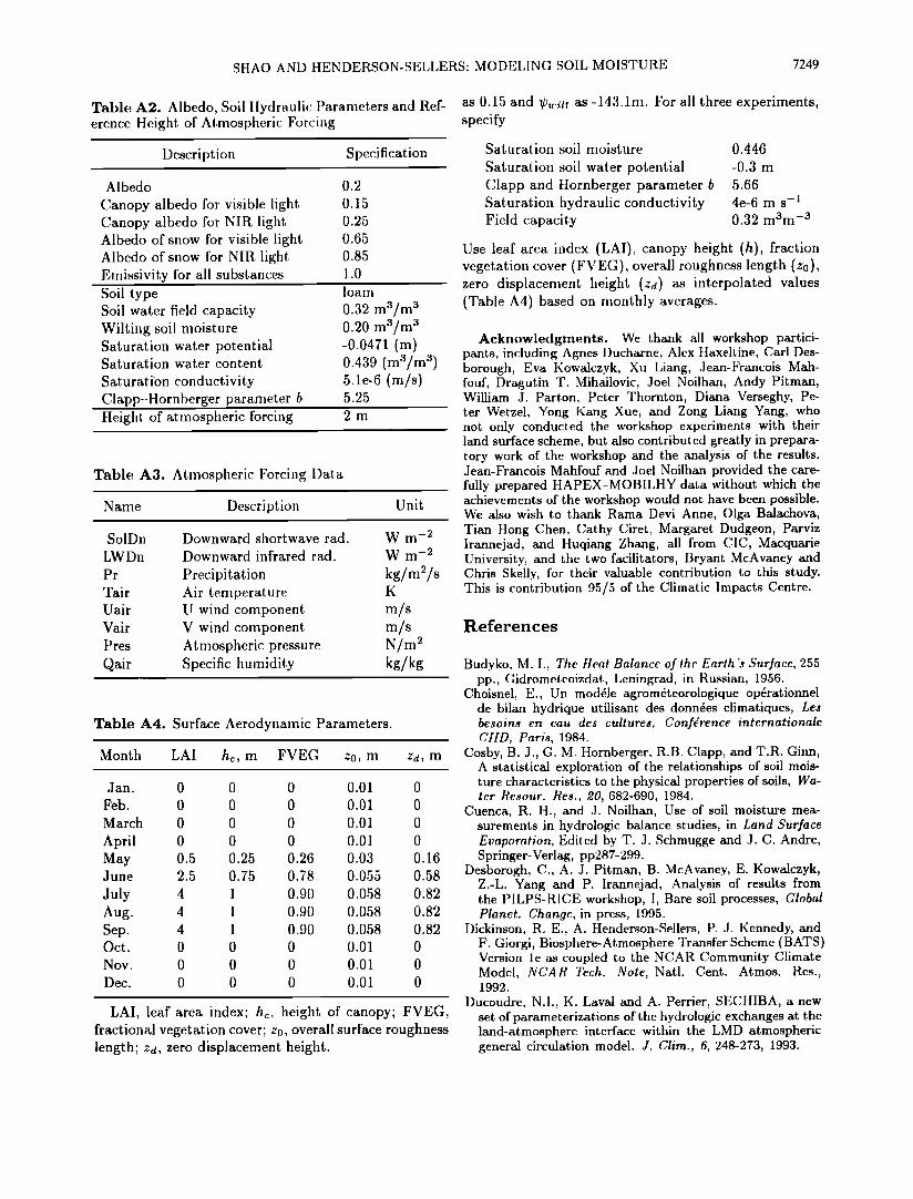
SHAO AND tIENDERSON-SELI,ERS: MODELING SOIL MOISTURE 7249

Table A2. Albedo, Soil Hydrauli(: Parameters and Ref- erence Height of Atmospheric Forcing

Descrip t ion S p ecificat ion

Albedo

Canopy albedo [or visible light, Canopy albedo for NIR light Albedo of snow for visible light Albedo of snow for NIR light, Emissivity for all substances

0.2

0.15

0.25

0.65

0.85

1.0

Soil type Soil water field capacity Wilting soil moisture Saturation water potential Saturation water content

Saturation conductivity Clapp Hornberger parameter b

foam

0.32 1113/1113 0.20 m3/m 3 -0.0471 (rn) 0.439 (m3/m 3) 5.1e-6 (m/s) 5.25

Height, of atmospheric forcing 2 m

Table A3. Atmospheric Forcing Data

Name Descr i pt ion Unit

SolDn Downward shortwave rad. LWDn Downward infrared tad.

Pr Precipitation Tair Air temperature Uair U wind component Vair V wind component Pres Atmospheric pressure Qair Specific humidity

W m -2 Wrn -•

kg/m•/s K

m/s m/s N/m_ 2 kg/kg

Table A4. Surface Aerodynamic Parameters.

Month LAI h•, m FVEG z0, m zd, m

Jan. 0 0 0 0.01 0

Feb. 0 0 0 0.01 0

March 0 0 0 0.01 0

April 0 0 0 0.01 0 May 0.5 0.25 0.26 0.03 0.16 June 2.5 0.75 0.78 0.055 0.58

July 4 1 0.90 0.0,58 0.82 Aug. 4 I 0.90 0.058 0.82 Sep. 4 1 0.90 0.058 0.82 Oct. 0 0 0 0.01 0

Nov. 0 0 0 0.01 0

Dec. 0 0 0 0.01 0

LAI, leaf area index; h•, height of canopy; FVEG, fractional vegetation cover; z0, overall surface roughness length; zd, zero displacement height.

as 0.15 and ;[',,..itt as-143.1m. For all three experiments, specify

Saturation soil moisture

Saturation soil water potential Clapp and }tornberger parameter b Saturation hydraulic conductivity Field capacity

0.446

-0.3 m

5.66

4e-6 m s-1 0.32 m3m -3

Use leaf area index (LAI), canopy height (h), fraction vegetation cover (FVEG), overall roughness length (z0), zero displacement height (zd) as interpolated values (Table A4) based on monthly averages.

Acknowle(lggnents. We thank all workshop participants, including Agnes Ducharne, Alex 1taxeltine, Carl Des- borough, Eva Kowalczyk, Xu Liang, Jean-Francois Mah- fouf, Dragutin T. Mihailovic, Joel Noilhan, Andy Pitman, William J. Parton, Peter Thornton, Diana Verseghy, Pe- ter Wetzel, Yong Kang Xue, and Zong Liang Yang, who not only conducted the workshop experiments with their land surface scheme, but also contributed greatly in prepara- tory work of the workshop and the analysis of the results. Jean-Francois Mahfouf and Joel Noilhan provided the care- fully prepared HAPEX-MOBILHY data without which the achievements of the workshop would not have been possible. We also wish to thank Rama Devi Anne, Olga Balachova, Tian Hong Chen, Cathy Ciret,, Margaret Dudgeon, Parviz Irannejad, and Huqiang Zhang, all from (?IC, Macquarie University, and the two facilitators, Bryant McAvaney and Chris Skelly, for their valuable contribution to this study. This is contribution 95/5 of the Climatic Impacts Centre.

References

Budyko, M. I., The Heat Balance of thc Earth's Surface, 255 pp., (;idromctcoizdat, Leningrad, in Russian, 1956.

Choisnel, E., Un modde agromdteorologique ope•rationnel de bilan hydrique utilisant des donnSes climatiques, Les besoins en eau des cultures, Confdrencc intcrnationale CIID, Paris, 1984.

Cosby, B. J., G. M. Hornberger, R.B. Clapp, and T.R. Ginn, A statistical exploration of the relationships of soil moisture characteristics to the physical properties of soils, Wa- ter Resour. Res., 20, 682-690, 1984.

Cuenca, R. H., and J. Noilhan, Use of soil moisture measurements in hydrologic balance studies, in Land Surface Evaporation, Edited by T. J. Schmugge and J. C. Andre, Springer-Verlag, pp287-299.

Desborogh, C., A. J. Pitman, B. McAvaney, E. Kowalczyk, Z.-L. Yang and P. Irannejad, Analysis of results from the PILPS-RICE workshop, I, Bare soil processes, Global Planet. Uhange, in press, 1995.

Dickinson, Fl. E., A. Henderson-Sellers, P. J. Kennedy, and F. Giorgi, Biosphere-Atmosphere Transfer Scheme (BATS) Version le as coupled to the NCAR Community Climate Model, NCAR Tech. Note, Natl. Cent. Atmos. Res., 1992.

Ducoudre, N.I., K. Laval and A. Perrier, SECHIBA, a new set of parameterizations of the hydrologic exchanges at the land-atmosphere interface within the LMD atmospheric general circulation model. J. Clirn., 6, 248-273, 1993.


Garratt, J. R., The Atmospheric Boundary Layer, 316 pp, Cambridge University Press.

Goutorbe, J.P., A critical assessment of the SAMER network accuracy, in Land Surface Evaporation, edited by T. J. Schmugge and J. C. Andre, 171-182, Springer-Verlag, New York, 1991.

Goutorbe, J.P., and C. Tarrieu, HAPEX-MOBILHY data base, in Land Surface Evaporation, edited by T. Schmugge and J. (7. Andre, 403-410, Springer-Verlag, New York, 1991.

Goutorbe, J. P., J. Noilhan, R. Cuenca, and (7. Valancogne, Soil moisture variations during ItAPEX-MOBILItY, Ann. Geophys., 7, 415-426, 1989.

Henderson-Sellers, A., A. J. Pitman, P. K. Love, P. lranne- jad, and T. H. Chen, The project, for intercomparison of land surface parameterization schemes (PlLPS): Phase 2 and 3, Bull. Am. Meteorol. Soc., 76, 489--503, 1995.

Jacquemin, B., and J. Noilhan, Sensitivity study of a land surface parameterization using the HAPEX-MOBILHY dataset, Boundary-Layer Meteorol., 5œ, 93-134, 1990.

Kowalczyk, E. A., J. R. Garratt, and P. B. Krummel, A soil-canopy scheme for use in a numerical model of the atmosphere- I D stand-alone model, CSIRO, DAR, Tech. Pap., œ3, 56 pp., Commonwealth Sci. and Ind. Res. Org., Melbourne, Victoria, 1991.

Liang, X., D. P. Lettenmaier, E. F. Wood, and S. J. Burges, A simple hydrologically based model of land surface water and energy fluxes for general circulation models, J. Geophys. Res., 99(I)7), 14,415-14,428, 1994.

Mahfouf J. F., A numerical simulation of the surface water budget during HAPEX-MOBILHY, Boundary-Layer Meteorol., 5.3, 201-222, 1990.

Mahfouf, J-F., C. Ciret, P. Irannejad, J. Noilhan, Y. Shao, P. Thornton, Y. Xue, and Z-L. Yang, Analysis of results from PILPS-RICE Workshop, III, Transpiration, Global Planet. Change, in press, 1995.

Manabe, S., Climate and Ocean circulation, 1, The atmospheric circulation and the hydrology of the earth's surface, Mon. Weather Rev., 97, 739-805, 1969.

Mihailovic, D. T., R. A. Pielke, B. Rajkovic, T. J. Lee, and M. Jeftic, A resistance representation of schemes for evaporation from bare and partly plant covered surfaces for use in atmospheric models, J. Appl. Meteorol., 3œ, 1038-1054, 1993.

Mihailovic, D. T., and B. Rajkovic, Soil moisture simulation with LAPS, Global Planet. Change, in press, 1995.

Noihlan, J., and S. Planton, A simple parameterization of land surface processes for meteorological models, Mon. Weather Rev., 117, 536-549, 1989.

Parton, W.J., et al., Observations and modeling of boimass and soil organic matter dynamics for the grassland biome worldwide, Global Biogeochem. Cycles, 7, 785-809, 1993.

Pitman, A. J., Z. L. Yang, J. G. Cogley, and A. Henderson- Sellers, Description of bare essentials of surface transfer for the Bureau of Meteorology Research Centre AGCM, BMRU Res. Rep. 3œ, 117 pp., Bur. of Meteorolol. Res. Cent., Melbourne, Victoria.

Pitman, A. J., et al., Results from the off-line control simulation phase of the Project for Intercomparison of Land Sur- face Parameterization Schemes (PlLPS), GEWEX Tech. Note, IGPO Publ. Series, 7, 47 pp.

Raupach, M. R., Simplified expressions for vegetation roughness length and zero-plane displacement as functions of canopy height and area index. Bou.ndary-Layer Meteo- rol., 71, 211-216, 1994.

Running, S. W., and E. R. ttunt .It., Gcncralization of a forest ecosystem process model for other biomes, BIOME- BGC, and an application for global-scale models, in Scal- ing Physiological Processes: Lea.[ to Globe, edited by J. R. Ehrlinger and C. Fields, Academic, San Diego, Calif., 1993.

Shao, Y., et al., Soil moisture simulation: a report of the RICE and PILPS workshop, GEWEX/GAIM Rep., IGPO Publication Series, 179 pp.

Verseghy, D. L., CLASS - a Canadian land surface scheme for GCMs, I, Soil model, Int.. J. Clim., 11, 111-133, 1991.

Verseghy, D. L., N. A. McFarlanc, and M. Lazare, CLASS- a Canadian land surface scheme for (?,CMs, II, Vegetation model and coupled runs, lnt. J. Clim., 13, 347-370, 1993.

Wetzel, P., and A. Boone, A parameterization for land- atmosphere-cloud exchange: Testing a detailed process model of the partly cloudy boundary layer over heterogeneous land. J. Ulim. 8, 1810-1837, 1995.

Wetzel, P. X. Liang, P. Irannejad, A. Boone, J. Noilhan, Y. Shao, (?. Skelly, Y. Xue, and Z. Yang, Modeling vadose zone liquid water fluxes: Infiltration, runoff, drainage, in- terflow, Global Planet. Change, in press, 1995.

Xue, Y., P. J. Sellers, J. L. Kinter and J. Shukla, A simplified biosphere model for global climate studies. J. Clim., 4, 345-364, 1991.

Yang, Z. L., R. E. Dickinson, A. Henderson-Sellers, and A. J. Pitman, Preliminary study of spin-up processes in land surface models, with the first stage data of PILPS phase la, J. Geophys. Res., 100, 16,553-16,578, 1995.

A. Henderson-Sellers, Climatic Impacts Centre, Macquarie University, Sydney, Australia. (e-mail: annC•cic.mq.edu.au)

Y. Shao, (lent. re for Advanced Numerical Computation in Engineering and Science, The University of New South Wales, Sydney, Australia. (e-mail: Y.Shao/•unsw.edu.au)

(Received Febrt•ary 9, 1995; revised September 11, 1995; accepted September 11, 1995.)

Modeling soil moisture: A Project for Intercomparison of ... · JOURNAL OF GEOPHYSICAL RESEARCH,...

Documents

Transcript of Modeling soil moisture: A Project for Intercomparison of ... · JOURNAL OF GEOPHYSICAL RESEARCH,...