
Modeling Problems in Constraint Programming
205
1 Modeling Problems in Constraint Programming Jean-Charles REGIN ILOG, Sophia Antipolis [email protected]
Transcript of Modeling Problems in Constraint Programming

1
Modeling Problems in Constraint Programming
Jean-Charles REGINILOG, Sophia Antipolis

2
Plan
❏ Principles of Constraint Programming❏ A rostering problem ❏ Modeling in CP: Principles❏ A difficult problem❏ A Network Design problem❏ Modeling Over-constrained problems❏ Discussion❏ Conclusion
3
3 problems
❏ 3 problems will be detailed:❍ A rostering problem (G. Pesant). This is a real world
problem. The problem is easy to solve in CP because all the needed constraints are available. The presentation will be constructive, that is the problem is modeled and described at the same time
❍ A part of a real world problem. Mainly a didactic problem which is difficult to solve in CP.
❍ A real world problem will be presented: a network design. First the whole problem will be described and then a CP solution will be proposed

4
Plan
❏ Principles of Constraint Programming❏ A rostering problem ❏ Modeling in CP: Principles❏ A difficult problem❏ A Network Design problem❏ Modeling Over-constrained problems❏ Discussion❏ Conclusion
5
Constraint programming
❏ Identify sub-problems that are easy (called constraints)
6
Constraint programming
❏ Identify sub-problems that are easy (called constraints)❏ 1) Use specific algorithm for solving these sub-problems and for
performing domain-reduction❏ 2) Instantiate a variable. Go to 1) and backtrack if necessary
7
Constraint programming
❏ Identify sub-problems that are easy (called constraints)❏ 1) Use specific algorithm for solving these sub-problems and for
performing domain-reduction❏ 2) Instantiate a variable. Go to 1) and backtrack if necessary❏ Local point of view on sub-problems. “Global” point of view by
propagation of domain reductions

8
Constraint Programming
❏ 3 notions:- constraint network: variables, domains, constraints + filtering (domain reduction)- propagation- search procedure (assignments + backtrack)
9
Problem = conjunction of sub-problems
❏ In CP a problem can be viewed as a conjunction of sub-problems that we are able to solve
❏ A sub-problem can be trivial: x < y or complex: search for a feasible flow
❏ A sub-problem = a constraint
10
Constraints
❏ Predefined constraints: arithmetic (x < y, x = y +z, |x-y| > k, alldiff, cardinality, sequence …
❏ Constraints given in extension by the list of allowed (or forbidden) combinations of values
❏ user-defined constraints: any algorithm can be encapsulated❏ Logical combination of constraints using OR, AND, NOT, XOR
operators. Sometimes called meta-constraints

11
Filtering
❏ We are able to solve a sub-problem: a method is available
❏ CP uses this method to remove values from domain that do not belong to a solution of this sub-problem: filtering
❏ E.g: x < y and D(x)=[10,20], D(y)=[5,15]=> D(x)=[10,14], D(y)=[11,15]
12
Filtering
❏ A filtering algorithm is associated with each constraint (sub-problem).
❏ Can be simple (x < y) or complex (alldiff)

13
Arc consistency
❏ All the values which do not belong to any solution of the constraint are deleted.
❏ Example: Alldiff({x,y,z}) with D(x)=D(y)={0,1}, D(z)={0,1,2}the two variables x and y take the values 0 and 1, thus z cannot take these values.FA by AC => 0 and 1 are removed from D(z)

14
Propagation
❏ Domain Reduction due to one constraint can lead to new domain reduction of other variables
❏ When a domain is modified all the constraints involving this variable are studied and so on ...

15
Why Propagation?
❏ A problem = conjunction of easy sub-problems. ❏ Sub-problems: local point of view. Propagation tries to
obtain a global point of view from independent local point of view
❏ The conjunction is stronger that the union of independent resolutions
16
Why Propagation?
❏ A problem = conjunction of easy sub-problems. ❏ Sub-problems: local point of view. Propagation tries to
obtain a global point of view from independent local point of view
❏ The conjunction is stronger that the union of independent resolution
❏ To help the propagation to have a global point of view: use global constraints !
❏ Global constraint = conjunction of constraints
17
Search
❏ Backtrack algorithm with strategies:try to successively assign variables with values. If a dead-end occurs then backtrack and try another value for the variable
❏ Strategy: define which variable and which value will be chosen.
❏ After each domain reduction (i.e assignment) filtering and propagation are triggered

18
Plan
❏ Principles of Constraint Programming❏ A rostering problem ❏ Modeling in CP: Principles❏ A difficult problem❏ A Network Design problem❏ Modeling Over-constrained problems❏ Discussion❏ Conclusion
19
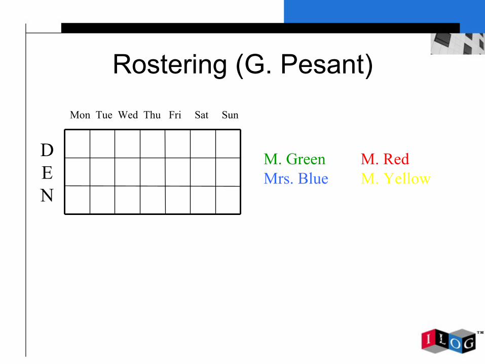
Rostering (G. Pesant)
Mon Tue Wed Thu Fri Sat Sun
DEN
M. Green M. RedMrs. Blue M. Yellow
20
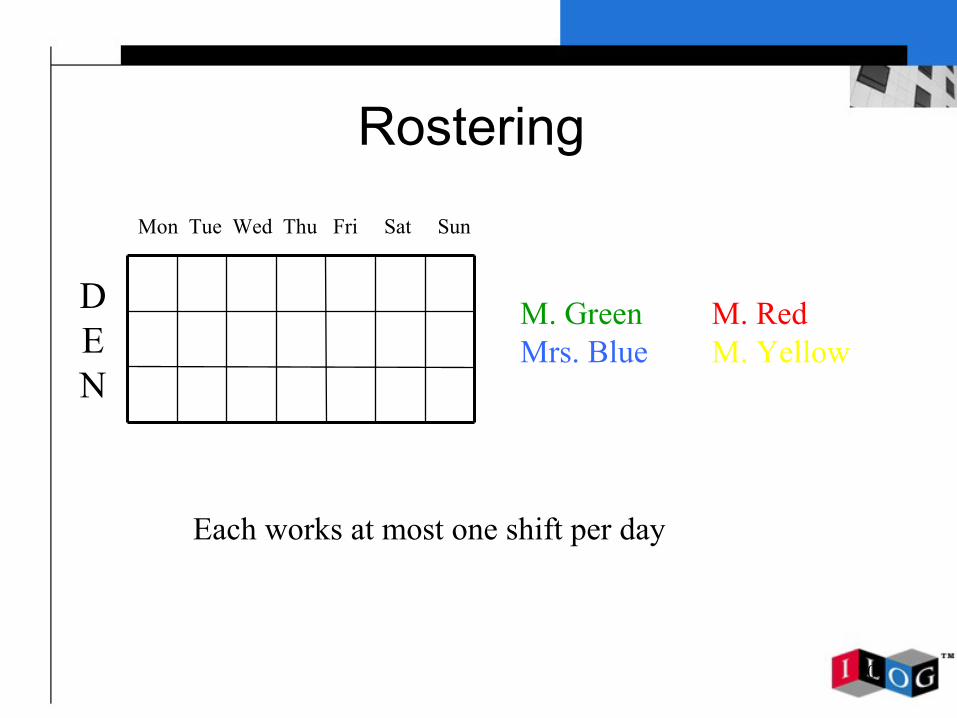
Rostering
Mon Tue Wed Thu Fri Sat Sun
DEN
M. Green M. RedMrs. Blue M. Yellow
Each works at most one shift per day

21
Rostering
Mon Tue Wed Thu Fri Sat Sun
DEN
M. Green M. RedMrs. Blue M. Yellow
xij ∈{g,b,r,y}
xiD ≠ xiE, xiD ≠ xiN, xiE ≠ xiN Mon ≤ i ≤ Sun

22
Rostering
Mon Tue Wed Thu Fri Sat Sun
DEN
enum Days = {mon,tue,wed,thu,fri,sat,sun}enum Shifts = {D,E,N}enum Workers = {green,white,red,yellow}var Workers onDuty[Days,Shifts]forall( i in Days )
forall( j,k in Shifts: j < k )onDuty[i,j] ≠ onDuty[i,k]
M. Green M. RedMrs. Blue M. Yellow

23
Rostering
Mon Tue Wed Thu Fri Sat Sun
DEN
enum Days = {mon,tue,wed,thu,fri,sat,sun}enum Shifts = {D,E,N}enum Workers = {green,white,red,yellow}var Workers onDuty[Days,Shifts]forall( i in Days )
forall( j,k in Shifts: j < k )onDuty[i,j] ≠ onDuty[i,k]
M. Green M. RedMrs. Blue M. Yellow

24
Mutual exclusion
❏ A set of variables must take on distinct values.❏ forall( i in Days )
forall( j,k in Shifts: j < k )onDuty[i,j] ≠ onDuty[i,k]

25
Mutual exclusion
❏ A set of variables must take on distinct values.❏ forall( i in Days )
forall( j,k in Shifts: j < k )onDuty[i,j] ≠ onDuty[i,k]
❏ Can be replaced byforall( i in Days )
alldifferent(onDuty[i])
26
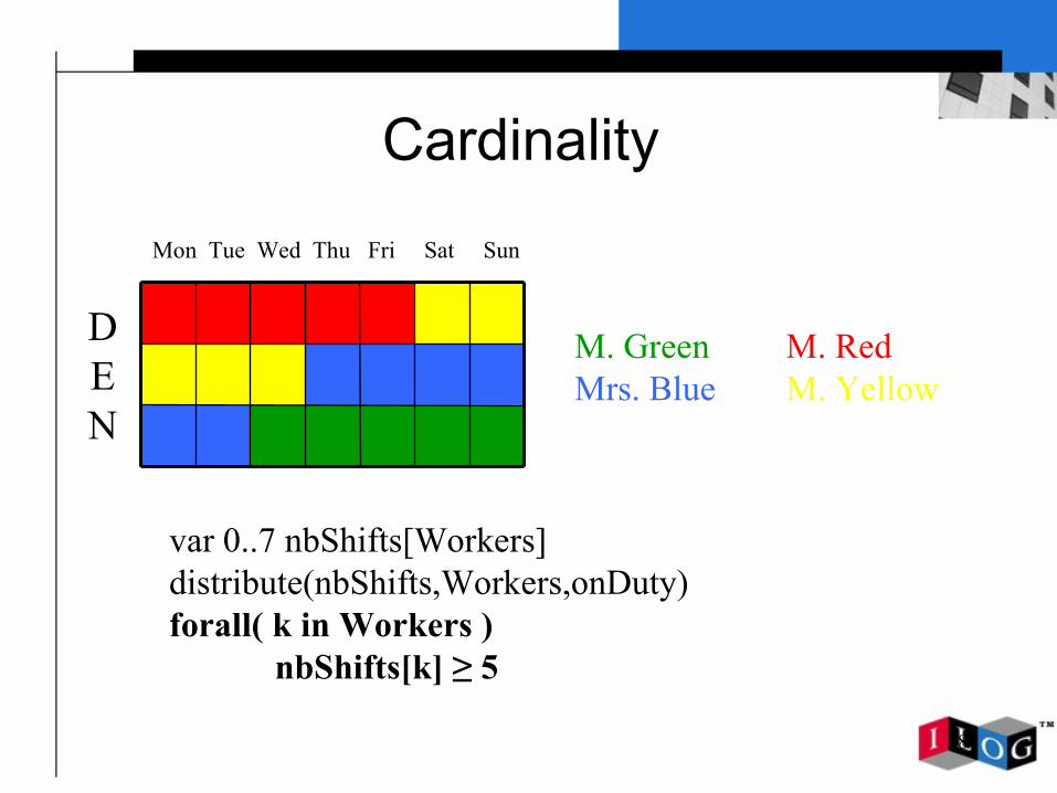
Cardinality
Mon Tue Wed Thu Fri Sat Sun
DEN
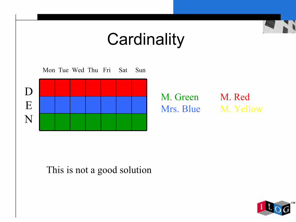
M. Green M. RedMrs. Blue M. Yellow
This is not a good solution

27
Cardinality
Mon Tue Wed Thu Fri Sat Sun
DEN
M. Green M. RedMrs. Blue M. Yellow
var 0..7 nbShifts[Workers]distribute(nbShifts,Workers,onDuty)forall( k in Workers )
nbShifts[k] ≥ 5
28
Cardinality
Mon Tue Wed Thu Fri Sat Sun
DEN
M. Green M. RedMrs. Blue M. Yellow
var 0..7 nbShifts[Workers]distribute(nbShifts,Workers,onDuty)forall( k in Workers )
nbShifts[k] ≥ 5

29
Dual Model
Mon Tue Wed Thu Fri Sat Sun
M. GreenMrs. BlueM. RedM. Yellow
enum Jobs = {D,E,N,-}var Jobs job[Days,Workers]
implicitly, each works at most one shift per day. But every job has to be performed and by only one worker

30
Dual Model
-
N
E
D
Mon Tue Wed Thu Fri Sat Sun
M. GreenMrs. BlueM. RedM. Yellow
implicitly, each works at most one shift per day. But every job is performed by only one worker forall( i in Days ) distribute([1,1,1,1],Jobs,job[i])
31
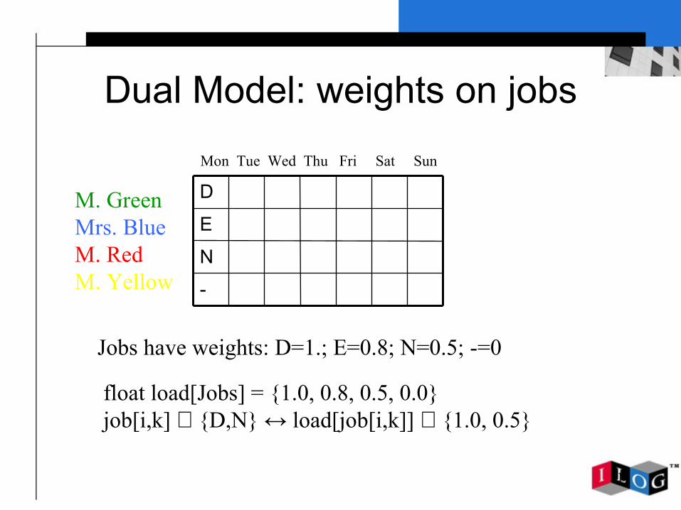
Dual Model: weights on jobs
-
N
E
D
Mon Tue Wed Thu Fri Sat Sun
M. GreenMrs. BlueM. RedM. Yellow
Jobs have weights: D=1.; E=0.8; N=0.5; -=0
float load[Jobs] = {1.0, 0.8, 0.5, 0.0}job[i,k] ∈ {D,N} ↔ load[job[i,k]] ∈ {1.0, 0.5}

32
Dual Model: weights on jobs
-
N
E
D
Mon Tue Wed Thu Fri Sat Sun
M. GreenMrs. BlueM. RedM. Yellow
Jobs have weights: D=1.; E=0.8; N=0.5; -=0
float load[Jobs] = {1.0, 0.8, 0.5, 0.0}forall( k in Workers )
sum( i in Days ) load[job[i,k]] ≥ 3.0
33
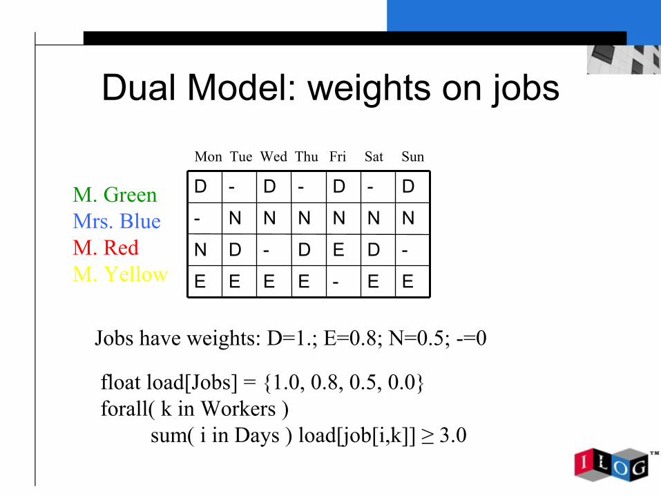
Dual Model: weights on jobs
EE-EEEE
-DED-DN
NNNNNN-
D-D-D-D
Mon Tue Wed Thu Fri Sat Sun
M. GreenMrs. BlueM. RedM. Yellow
Jobs have weights: D=1.; E=0.8; N=0.5; -=0
float load[Jobs] = {1.0, 0.8, 0.5, 0.0}forall( k in Workers )
sum( i in Days ) load[job[i,k]] ≥ 3.0

34
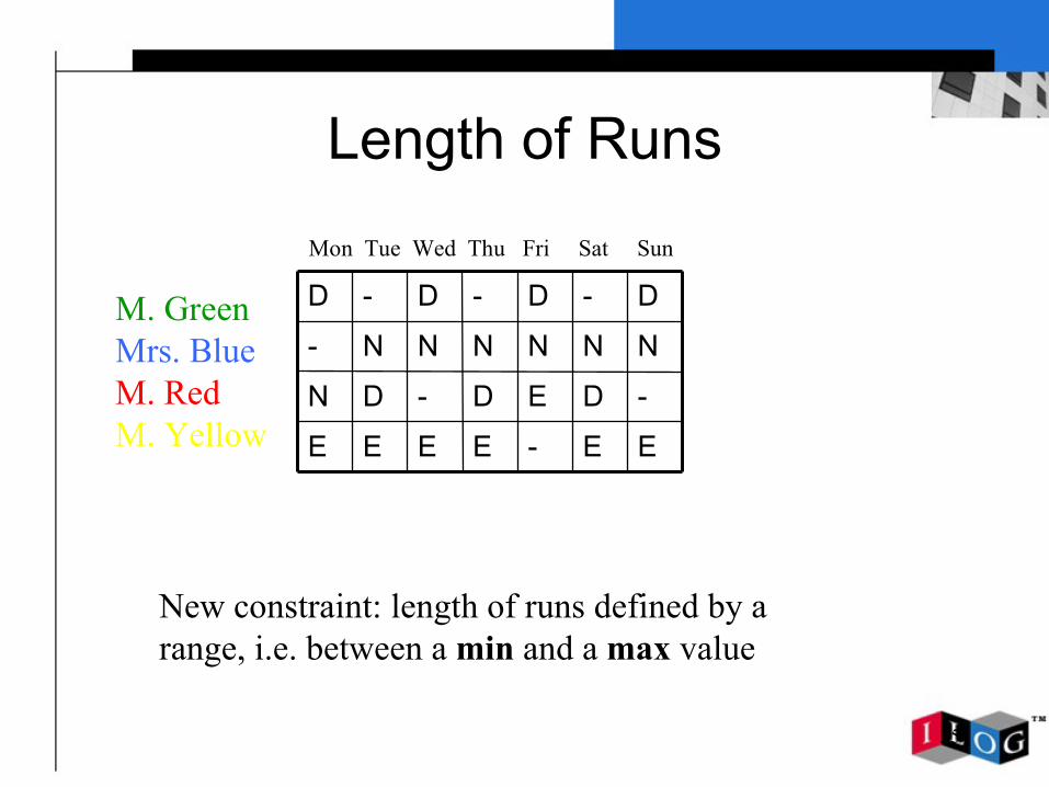
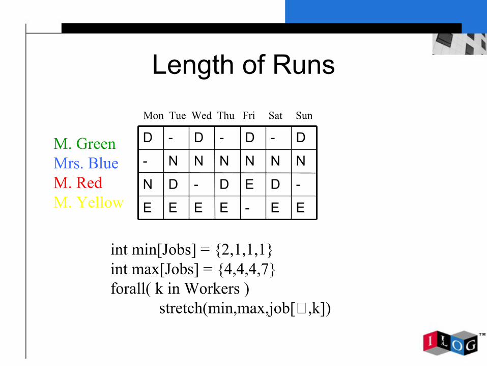
Length of Runs
EE-EEEE
-DED-DN
NNNNNN-
D-D-D-D
Mon Tue Wed Thu Fri Sat Sun
M. GreenMrs. BlueM. RedM. Yellow
This is not nice, isn’t it?
35
Length of Runs
EE-EEEE
-DED-DN
NNNNNN-
D-D-D-D
Mon Tue Wed Thu Fri Sat Sun
M. GreenMrs. BlueM. RedM. Yellow
New constraint: length of runs defined by a range, i.e. between a min and a max value
36
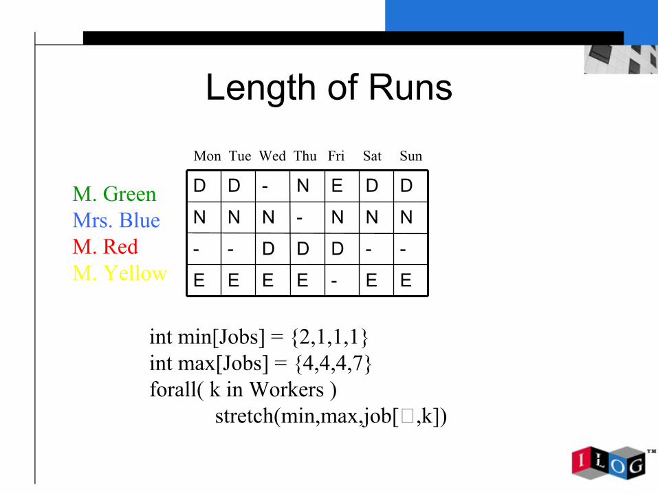
Length of Runs
EE-EEEE
-DED-DN
NNNNNN-
D-D-D-D
Mon Tue Wed Thu Fri Sat Sun
M. GreenMrs. BlueM. RedM. Yellow
int min[Jobs] = {2,1,1,1}int max[Jobs] = {4,4,4,7}forall( k in Workers )
stretch(min,max,job[⋆,k])
37
Length of Runs
EE-EEEE
--DDD--
NNN-NNN
DDEN-DD
Mon Tue Wed Thu Fri Sat Sun
M. GreenMrs. BlueM. RedM. Yellow
int min[Jobs] = {2,1,1,1}int max[Jobs] = {4,4,4,7}forall( k in Workers )
stretch(min,max,job[⋆,k])

38
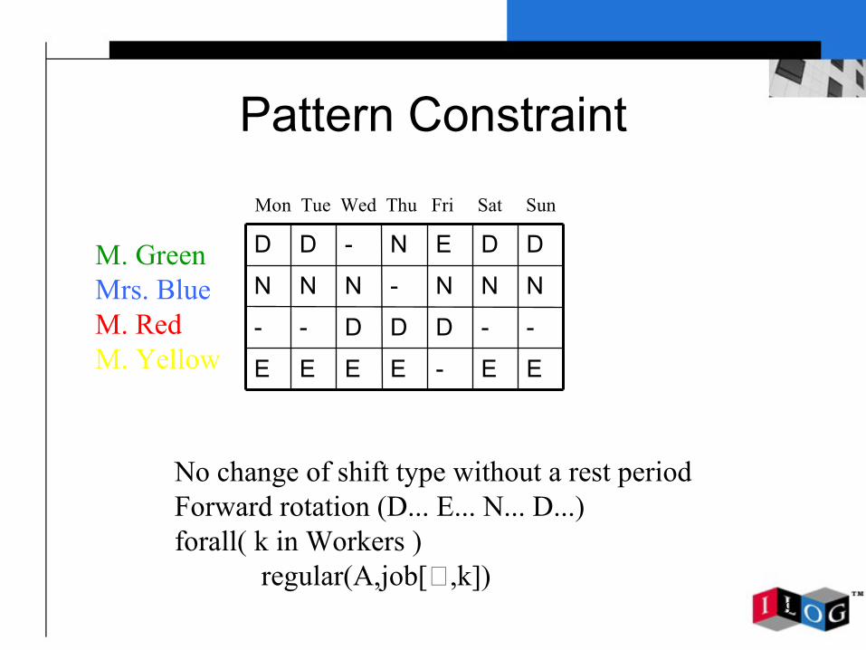
Pattern Constraint
EE-EEEE
--DDD--
NNN-NNN
DDEN-DD
Mon Tue Wed Thu Fri Sat Sun
M. GreenMrs. BlueM. RedM. Yellow
No change of shift type without a rest periodForward rotation (D... E... N... D...)
39
Pattern Constraint
EE-EEEE
--DDD--
NNN-NNN
DDEN-DD
Mon Tue Wed Thu Fri Sat Sun
M. GreenMrs. BlueM. RedM. Yellow
No change of shift type without a rest periodForward rotation (D... E... N... D...)forall( k in Workers )
regular(A,job[⋆,k])

40
Pattern Constraint
--DDD--
DD-NNNN
NNN-EEE
EEEE-DD
Mon Tue Wed Thu Fri Sat Sun
M. GreenMrs. BlueM. RedM. Yellow
No change of shift type without a rest periodForward rotation (D... E... N... D...)forall( k in Workers )
regular(A,job[⋆,k])
41
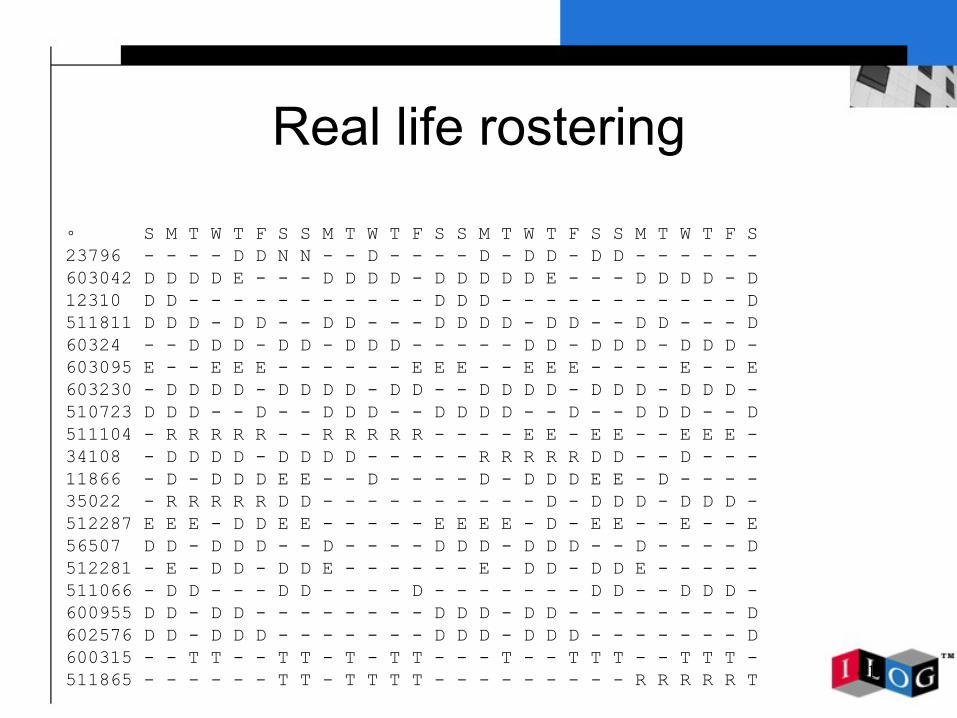
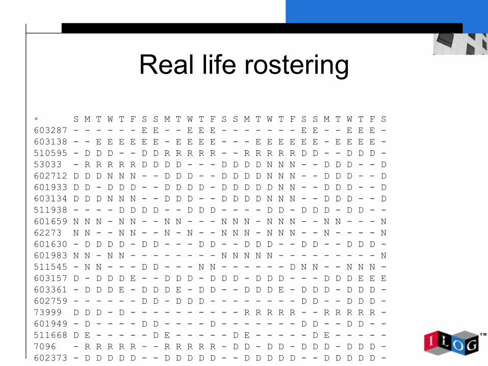
Real life rostering
◦ S M T W T F S S M T W T F S S M T W T F S S M T W T F S23796 - - - - D D N N - - D - - - - D - D D - D D - - - - - -603042 D D D D E - - - D D D D - D D D D D E - - - D D D D - D12310 D D - - - - - - - - - - - D D D - - - - - - - - - - - D511811 D D D - D D - - D D - - - D D D D - D D - - D D - - - D60324 - - D D D - D D - D D D - - - - - D D - D D D - D D D -603095 E - - E E E - - - - - - E E E - - E E E - - - - E - - E603230 - D D D D - D D D D - D D - - D D D D - D D D - D D D -510723 D D D - - D - - D D D - - D D D D - - D - - D D D - - D511104 - R R R R R - - R R R R R - - - - E E - E E - - E E E -34108 - D D D D - D D D D - - - - - R R R R R D D - - D - - -11866 - D - D D D E E - - D - - - - D - D D D E E - D - - - -35022 - R R R R R D D - - - - - - - - - - D - D D D - D D D -512287 E E E - D D E E - - - - - E E E E - D - E E - - E - - E56507 D D - D D D - - D - - - - D D D - D D D - - D - - - - D512281 - E - D D - D D E - - - - - - E - D D - D D E - - - - -511066 - D D - - - D D - - - - D - - - - - - - D D - - D D D -600955 D D - D D - - - - - - - - D D D - D D - - - - - - - - D602576 D D - D D D - - - - - - - D D D - D D D - - - - - - - D600315 - - T T - - T T - T - T T - - - T - - T T T - - T T T -511865 - - - - - - T T - T T T T - - - - - - - - - R R R R R T
42
Real life rostering
◦ S M T W T F S S M T W T F S S M T W T F S S M T W T F S603287 - - - - - - E E - - E E E - - - - - - - E E - - E E E -603138 - - E E E E E E - E E E E - - - E E E E E E - E E E E -510595 - D D D - - D D R R R R R - - R R R R R D D - - D D D -53033 - R R R R R D D D D - - - D D D D N N N - - D D D - - D602712 D D D N N N - - D D D - - D D D D N N N - - D D D - - D601933 D D - D D D - - D D D D - D D D D D N N - - D D D - - D603134 D D D N N N - - D D D - - D D D D N N N - - D D D - - D511938 - - - - D D D D - - D D D - - - - D D - D D D - D D - -601659 N N N - N N - - N N - - - N N N - N N N - - N N - - - N62273 N N - - N N - - N - N - - N N N - N N N - - N - - - - N601630 - D D D D - D D - - - D D - - D D D - - D D - - D D D -601983 N N - N N - - - - - - - - N N N N N - - - - - - - - - N511545 - N N - - - D D - - - N N - - - - - - D N N - - N N N -603157 D - D D D E - - D D D - D D D - D D D - - - D D D E E E603361 - D D D E - D D D E - D D - - D D D E - D D D - D D D -602759 - - - - - - D D - D D D - - - - - - - - D D - - D D D -73999 D D D - D - - - - - - - - - - R R R R R - - R R R R R -601949 - D - - - - D D - - - - D - - - - - - - D D - - D D - -511668 D E - - - - - D E - - - - - D E - - - - - D E - - - - -7096 - R R R R R - - R R R R R - D D - D D - D D D - D D D -602373 - D D D D D - - D D D D D - - D D D D D - - D D D D D -
43
Plan
❏ Principles of Constraint Programming❏ A rostering problem ❏ Modeling in CP: Principles❏ A difficult problem❏ A Network Design problem❏ Modeling Over-constrained problems❏ Discussion❏ Conclusion
44
Modeling: principles
❏ What a good model is?❏ Symmetries❏ Implicit constraints❏ Global constraints❏ Relevant and redundant constraints❏ Back propagation❏ Dominance rules

45
Good Model?
❏ A good model is a model that leads to an efficient resolution of a given problem

46
Good Model?
❏ A good model is a model that leads to an efficient resolution of a given problem
❏ Deals with several notions:
SymmetriesImplicit constraintsGlobal constraints
Relevant and redundant constraintsBack propagationDominance rules

47
Symmetries
❏ Tutorial on this topic at CP’04❏ The complexity of a problem can often be reduced by detecting
intrinsic symmetries❏ When two or more variables have identical characteristics, it is
pointless to differentiate them artificially:❍ The initial domains of these variables are identical❍ These variables are subject to the same constraints❍ The variables can be permuted without changing the statement of
the problem❏ Usually symmetries are removed by introducing an order
between variables

48
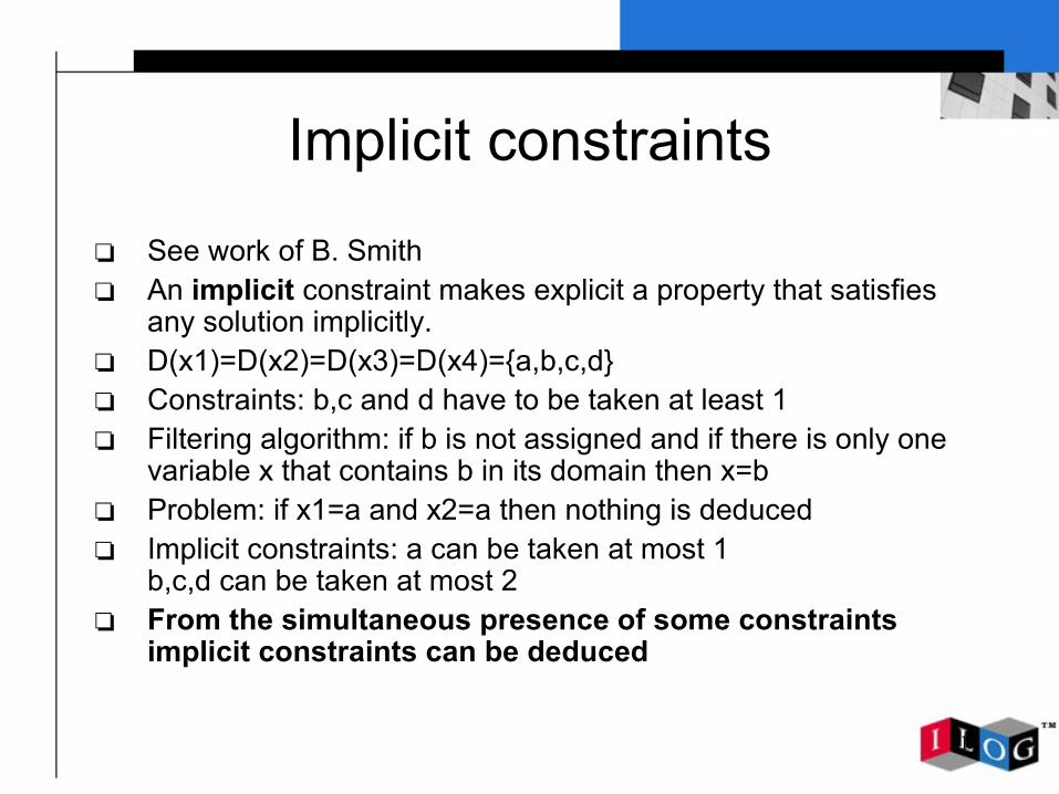
Implicit constraints
❏ See work of B. Smith❏ An implicit constraint makes explicit a property that
satisfies any solution implicitly.❏ D(x1)=D(x2)=D(x3)=D(x4)={a,b,c,d}❏ Constraints: b,c and d have to be taken at least 1

49
Implicit constraints
❏ See work of B. Smith❏ An implicit constraint makes explicit a property that
satisfies any solution implicitly.❏ D(x1)=D(x2)=D(x3)=D(x4)={a,b,c,d}❏ Constraints: b,c and d have to be taken at least 1❏ Filtering algorithm: if b is not assigned and if there is
only one variable x that contains b in its domain then x=b
50
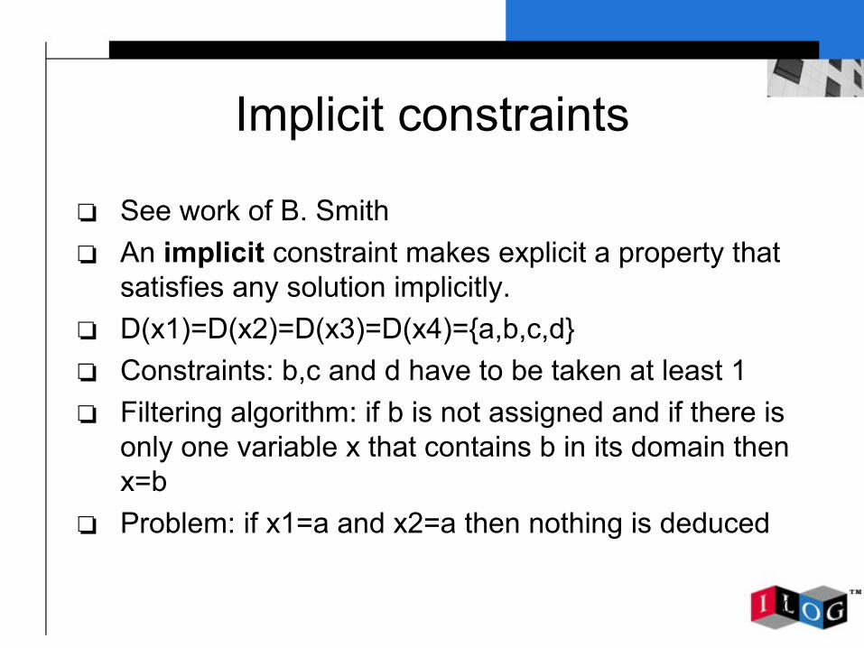
Implicit constraints
❏ See work of B. Smith❏ An implicit constraint makes explicit a property that
satisfies any solution implicitly.❏ D(x1)=D(x2)=D(x3)=D(x4)={a,b,c,d}❏ Constraints: b,c and d have to be taken at least 1❏ Filtering algorithm: if b is not assigned and if there is
only one variable x that contains b in its domain then x=b
❏ Problem: if x1=a and x2=a then nothing is deduced
51
Implicit constraints
❏ See work of B. Smith❏ An implicit constraint makes explicit a property that satisfies
any solution implicitly.❏ D(x1)=D(x2)=D(x3)=D(x4)={a,b,c,d}❏ Constraints: b,c and d have to be taken at least 1❏ Filtering algorithm: if b is not assigned and if there is only one
variable x that contains b in its domain then x=b❏ Problem: if x1=a and x2=a then nothing is deduced❏ Implicit constraints: a can be taken at most 1
b,c,d can be taken at most 2❏ From the simultaneous presence of some constraints
implicit constraints can be deduced

52
Global constraints
❏ A global constraint is a conjunction of constraints. This conjunction often takes into account implicit constraint deduced from the simultaneous presence of the other constraints
❏ This is the case for the previous example with the global cardinality constraint
❏ Use the strongest filtering algorithm as you can at the beginning
❏ It is rare to be able to solve a problem with weak FA and not to be able to solve it with strong FA

53
Global constraint: Alldiff results
❏ Color the graph with cliques:c0 = {0, 1, 2, 3, 4} c1 = {0, 5, 6, 7, 8}c2 = {1, 5, 9, 10, 11}c3 = {2, 6, 9, 12, 13} c4 = {3, 7, 10, 12, 14} c5 = {4, 8, 11, 13, 14}
❏ clique size:27 Global: #fails: 0 cpu time: 1.212 sLocal: #fails: 1 cpu time: 0.171 s
clique size:31 Global: #fails: 4 cpu time: 2.263 sLocal: #fails: 65 cpu time: 0.37 s
clique size:51 Global: #fails: 501 cpu time: 25.947 sLocal: #fails: 24512 cpu time: 66.485 s
clique size:61 Global: #fails: 5 cpu time: 58.223 sLocal: ?????????????
54
Relevant Constraints
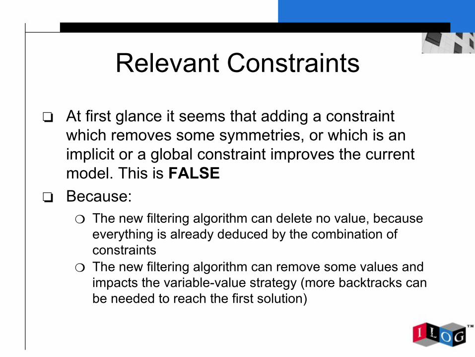
❏ At first glance it seems that adding a constraint which removes some symmetries, or which is an implicit or a global constraint improves the current model. This is FALSE
❏ Because:❍ The new filtering algorithm can delete no value, because
everything is already deduced by the combination of constraints
❍ The new filtering algorithm can remove some values and impacts the variable-value strategy (more backtracks can be needed to reach the first solution)
55
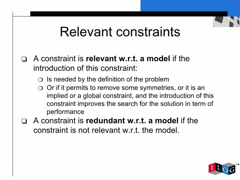
Relevant constraints
❏ A constraint is relevant w.r.t. a model if the introduction of this constraint:
❍ Is needed by the definition of the problem❍ Or if it permits to remove some symmetries, or it is an
implied or a global constraint, and the introduction of this constraint improves the search for the solution in term of performance
❏ A constraint is redundant w.r.t. a model if the constraint is not relevant w.r.t. the model.
56
Back propagation
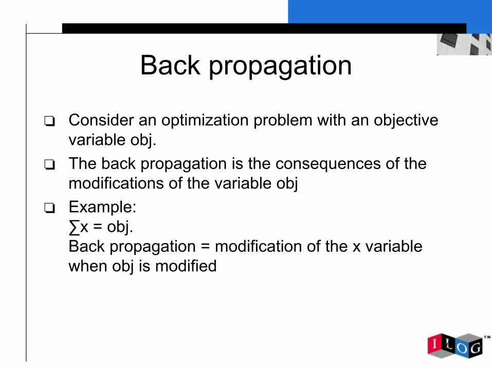
❏ Consider an optimization problem with an objective variable obj.
❏ The back propagation is the consequences of the modifications of the variable obj
❏ Example:∑x = obj. Back propagation = modification of the x variable when obj is modified
57
Back propagation
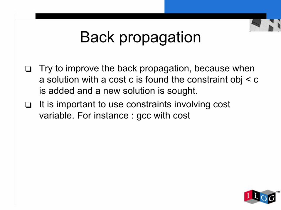
❏ Try to improve the back propagation, because when a solution with a cost c is found the constraint obj < c is added and a new solution is sought.
❏ It is important to use constraints involving cost variable. For instance : gcc with cost
58
Dominance rules
❏ A dominance rule is a rule that eliminates some solutions that are not optimal, or some optimal solutions but not all
❏ This is a kind of symmetry breaking in regards to the optimality
❏ An example is given in the resolution of the next problem
59
A bad model?
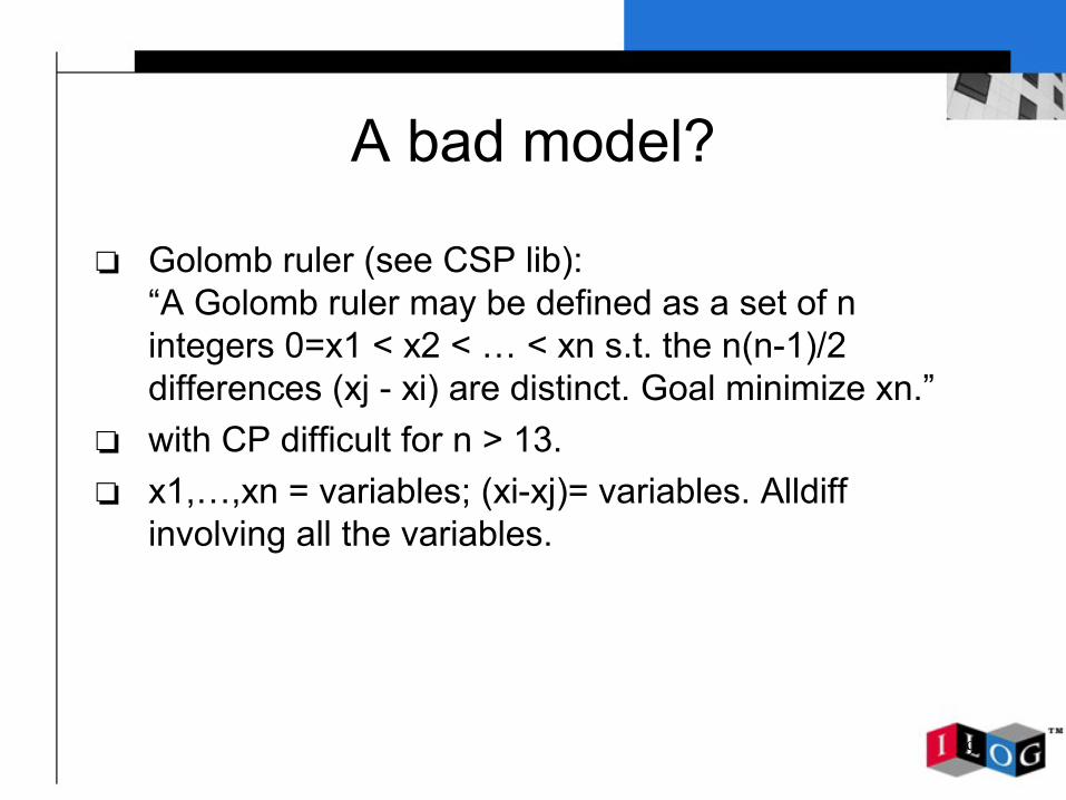
❏ Golomb ruler (see CSP lib):“A Golomb ruler may be defined as a set of n integers 0=x1 < x2 < … < xn s.t. the n(n-1)/2 differences (xj - xi) are distinct. Goal minimize xn.”
❏ with CP difficult for n > 13.❏ x1,…,xn = variables; (xi-xj)= variables. Alldiff
involving all the variables.

60
Alldiff
|x1-x2|
|x1-x3|
|x2-x3|
x1
x2
x3
1
2
3
4
5
6
7
Not a good solutionBad incorporationof constraint|xi – xj| in alldiff

61
Plan
❏ Principles of Constraint Programming❏ A rostering problem ❏ Modeling in CP: Principles❏ A difficult problem❏ A Network Design problem❏ Modeling Over-constrained problems❏ Discussion❏ Conclusion
62
Even Round Robin
- 1- 6+ 4- 2+ 7- 5+ 38
+ 2+ 1- 5+ 3- 8+ 6- 47
- 3+ 8- 1- 4+ 2- 7+ 56
+ 4- 2+ 7+ 1- 3+ 8- 65
- 5+ 3- 8+ 6- 1- 2+ 74
+ 6- 4+ 2- 7+ 5+ 1- 83
- 7+ 5- 3+ 8- 6+ 4- 12
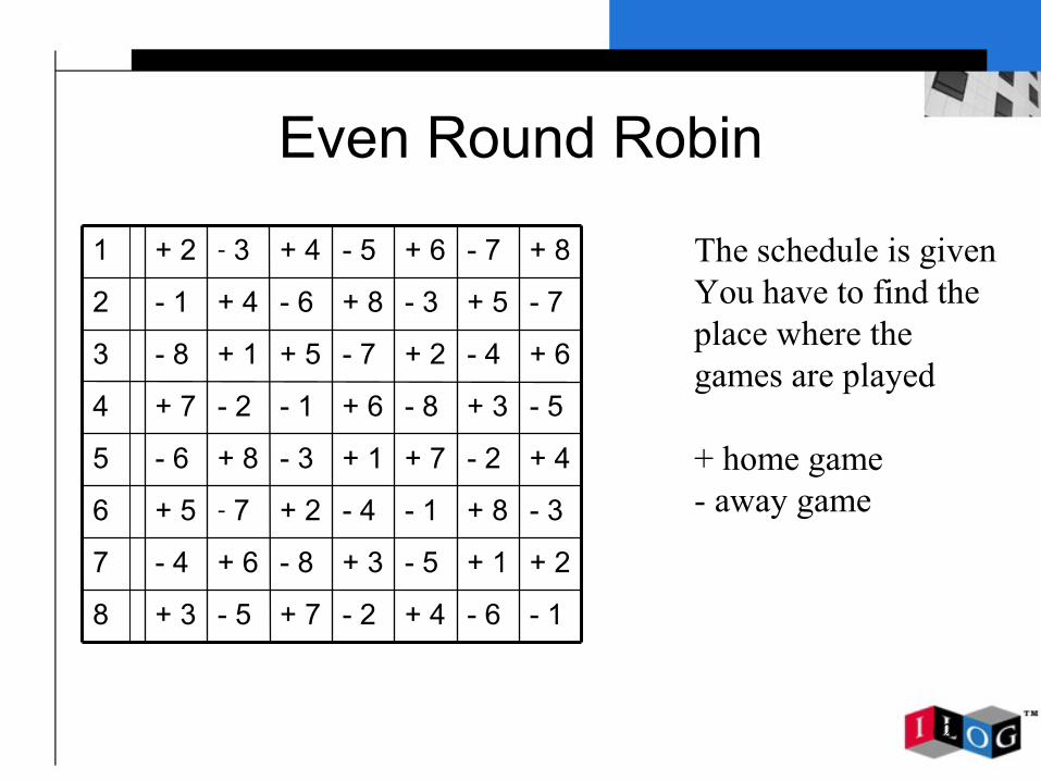
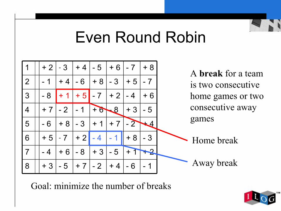
+ 8- 7+ 6- 5+ 4- 3+ 21 The schedule is given You have to find the place where the games are played
+ home game- away game
63
Even Round Robin
- 1- 6+ 4- 2+ 7- 5+ 38
+ 2+ 1- 5+ 3- 8+ 6- 47
- 3+ 8- 1- 4+ 2- 7+ 56
+ 4- 2+ 7+ 1- 3+ 8- 65
- 5+ 3- 8+ 6- 1- 2+ 74
+ 6- 4+ 2- 7+ 5+ 1- 83
- 7+ 5- 3+ 8- 6+ 4- 12
+ 8- 7+ 6- 5+ 4- 3+ 21A break for a team is two consecutive home games or two consecutive away games
Home break
Away break
Goal: minimize the number of breaks
64
Model: Variables
- 1- 6+ 4- 2+ 7- 5+ 38
+ 2+ 1- 5+ 3- 8+ 6- 47
- 3+ 8- 1- 4+ 2- 7+ 56
+ 4- 2+ 7+ 1- 3+ 8- 65
- 5+ 3- 8+ 6- 1- 2+ 74
+ 6- 4+ 2- 7+ 5+ 1- 83
- 7+ 5- 3+ 8- 6+ 4- 12
+ 8- 7+ 6- 5+ 4- 3+ 21
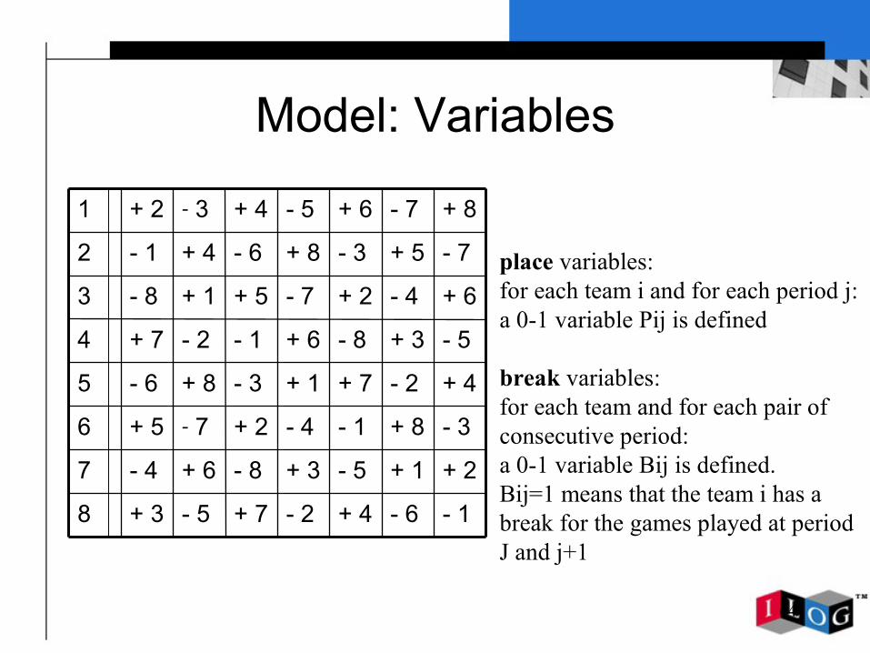
place variables: for each team i and for each period j: a 0-1 variable Pij is defined
break variables:for each team and for each pair ofconsecutive period:a 0-1 variable Bij is defined.Bij=1 means that the team i has a break for the games played at periodJ and j+1

65
Model: Objective
- 1- 6+ 4- 2+ 7- 5+ 38
+ 2+ 1- 5+ 3- 8+ 6- 47
- 3+ 8- 1- 4+ 2- 7+ 56
+ 4- 2+ 7+ 1- 3+ 8- 65
- 5+ 3- 8+ 6- 1- 2+ 74
+ 6- 4+ 2- 7+ 5+ 1- 83
- 7+ 5- 3+ 8- 6+ 4- 12
+ 8- 7+ 6- 5+ 4- 3+ 21 Objective Variable:
#B is the variable that counts thetotal number of breaks for the schedule

66
Model: Constraints
- 1- 6+ 4- 2+ 7- 5+ 38
+ 2+ 1- 5+ 3- 8+ 6- 47
- 3+ 8- 1- 4+ 2- 7+ 56
+ 4- 2+ 7+ 1- 3+ 8- 65
- 5+ 3- 8+ 6- 1- 2+ 74
+ 6- 4+ 2- 7+ 5+ 1- 83
- 7+ 5- 3+ 8- 6+ 4- 12
+ 8- 7+ 6- 5+ 4- 3+ 21 place-opponent constraint:i plays k at home at period j is equivalent tok plays i away at period j
break constraint:if a team i plays for two consecutive periods j and j+1 at home or away then Bij=1 and conversly.
#B=∑i∑j Bij (i=1..n, j=1..n-2)

67
First test
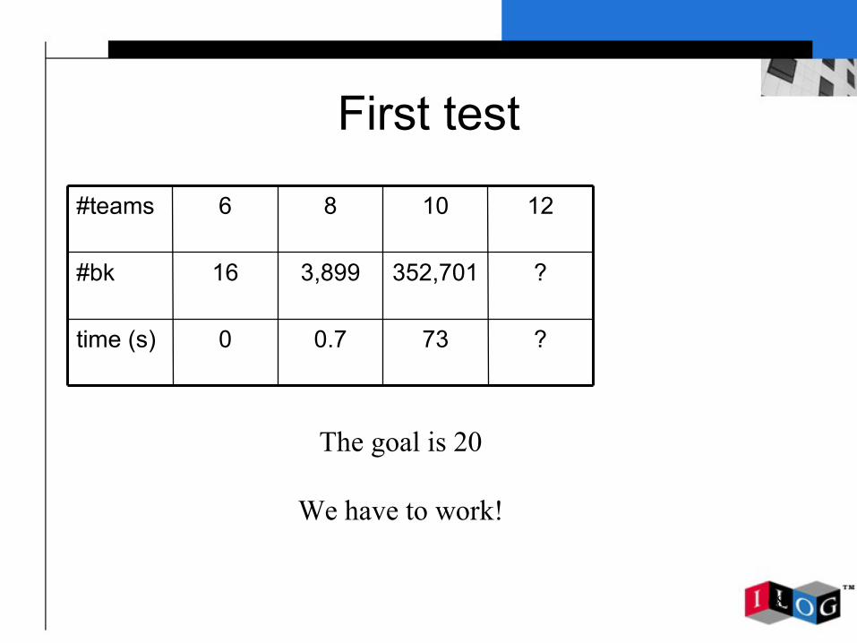
?730.70time (s)
?352,7013,89916#bk
121086#teams
68
First test
?730.70time (s)
?352,7013,89916#bk
121086#teams
The goal is 20
We have to work!
69
Symmetry?
- 1- 6+ 4- 2+ 7- 5+ 38
+ 2+ 1- 5+ 3- 8+ 6- 47
- 3+ 8- 1- 4+ 2- 7+ 56
+ 4- 2+ 7+ 1- 3+ 8- 65
- 5+ 3- 8+ 6- 1- 2+ 74
+ 6- 4+ 2- 7+ 5+ 1- 83
- 7+ 5- 3+ 8- 6+ 4- 12
+ 8- 7+ 6- 5+ 4- 3+ 21
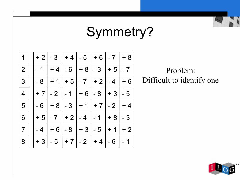
Problem:Difficult to identify one

70
Study of the problem
❏ There is no schedule with less than n-2 breaks❏ Proof: consider 2 teams a, b
Assume a has no breakAssume b has no break: this means that a and b “alternate” (a is + - + - + - … and b is - + - + - + …)because a plays b at a moment.Now consider any other team c, then c has necessarily a break because c cannot alternate simultaneously with a and with b

71
N-2 as lower bound
❏ If the minimal value is close to n-2 then it is more interesting to try successively the values from n-2 w.r.t. an increasing order than finding a first solution and then trying to reduce the objective value

72
Relevant constraints
❏ For each two consecutive periods the number of away break (- -) is equal to the number of home breaks (+ +)
❏ Proof: for each period the number of + is equal to the number of -. We cannot have an odd number of non breaks.
❏ Corollary: #B is even --
+-
++
-+
73
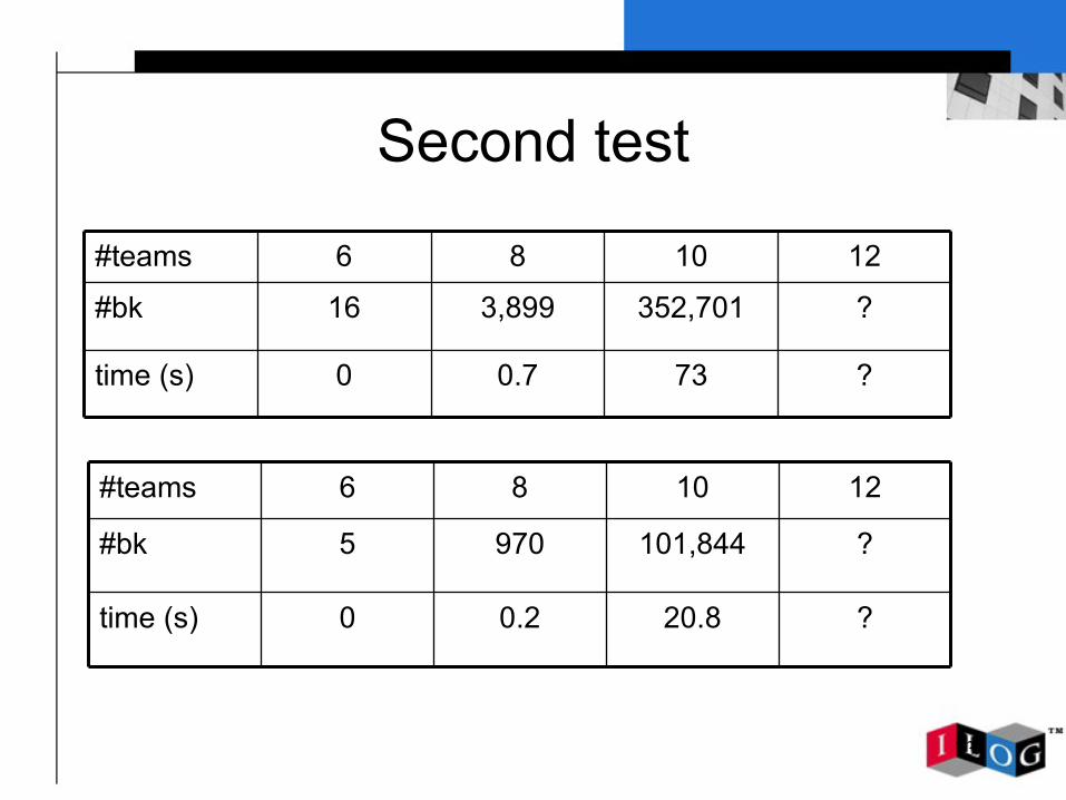
Second test
?730.70time (s)
?352,7013,89916#bk
121086#teams
?20.80.20time (s)
?101,8449705#bk
121086#teams

74
Relevant constraints
❏ Suppose that for a team we have+ . - . . . .and exactly one break is requiredthen we can deduce: + . - + - + -
❏ Property: #Bi(j,k): number of break for team i between period j and k
j a period, k a period with k = j + qPij=Pik ⇔ #Bi(j,k) has the parity of q

75
Third test
??20.80.2time (s)
??101,844970#bk
1412108#teams
?55.34.00.1time (s)
?135,12911,542226#bk
1412108#teams
76
Relevant constraint
❏ As proved at the beginning: there are at most two teams with no break

77
Fourth test
?55.34.00.1time (s)
?135,12911,542226#bk
1412108#teams
904.41.370.40.1time (s)
1,716,5132,43584641#bk
1412108#teams

78
Variable-value strategy
❏ Strategy:1) The #Bi variables with domain-min2) The place variables for the first period3) the break variables by trying first value 14) the place variables

79
Fifth test
904.41.370.40.1time (s)
1,716,5132,43584641#bk
1412108#teams
397.11.180.40.1time (s)
711,4082,20984641#bk
1412108#teams

80
Dominance rules
+ y- ij
- x+ ji
y- ij
x+ ji
- y- ij
- x+ ji
- y- ij
+ x+ ji
+ y- ij
+ x+ jibreak break
break
break

81
Dominance rules
+ y- ij
- x+ ji
- y- ij
- x+ ji
- y- ij
+ x+ ji
+ y- ij
+ x+ jibreak break
break
break
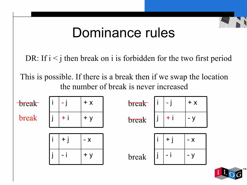
DR: If i < j then break on i is forbidden for the two first period
82
Dominance rules
+ y- ij
- x+ ji
- y- ij
- x+ ji
- y+ ij
+ x- ji
+ y+ ij
+ x- jibreak break
break
break
DR: If i < j then break on i is forbidden for the two first period
This is possible. If there is a break then if we swap the location the number of break is never increased
break
83
Dominance rules
❏ The dominance rule can be defined for the first two column and for the last two columns
❏ It is also possible to define dominance rules for the middle, but this is quite complex.
84
Final result
❏ 16 teams in 5s❏ 18 teams in 20s❏ 20 teams in 200s
85
Plan
❏ Principles of Constraint Programming❏ A rostering problem ❏ Modeling in CP: Principles❏ A difficult problem❏ A Network Design problem❏ Modeling Over-constrained problems❏ Discussion❏ Conclusion

86
The ROCOCO Project
❏ France Telecom R&D ISE❍ Problem and benchmark definition❍ Algorithm validation
❏ Research laboratories: INRIA Numopt, LRI Orsay, PRiSM Versailles, Evry, …
❍ Lower bounds: Lagrangean relaxation, column generation, cuts
❍ Optimization techniques: genetic algorithms❏ ILOG
❍ Optimization techniques: constraint programming, mixed integer programming, column generation
87
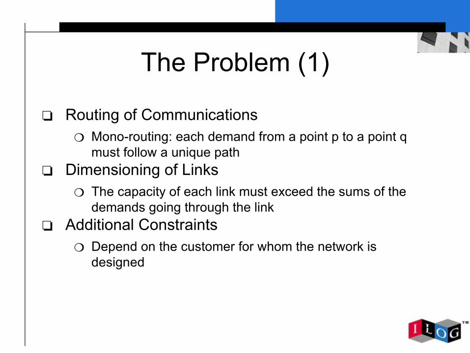
The Problem (1)
❏ Routing of Communications❍ Mono-routing: each demand from a point p to a point q
must follow a unique path❏ Dimensioning of Links
❍ The capacity of each link must exceed the sums of the demands going through the link
❏ Additional Constraints❍ Depend on the customer for whom the network is
designed

88
The Problem (2)Data:
• Customer traffic demands
• Possible links, capacities and costs
S1 S2
S3
S4
S1S2
S3
S4
Result:❍ Minimal cost
network able to simultaneously respond to all the demands
❍ Route for each demand
27Kb/s
115Kb/s
Rented capacity 256Kb/s

89
The Problem (3)
❏ Cost minimization principle❍ Traffic demands share link capacities
S1 S2
S3
512Kb/s128Kb/s
115Kb/s
256Kb/s
90
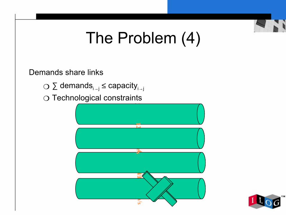
The Problem (4)
Demands share links
❍ ∑ demandsi→j ≤ capacityi→j
❍ Technological constraints256Kb/s
64Kb/s
64Kb/s
64Kb/s
64Kb/s
128Kb/s
128Kb/s
64Kb/s
64Kb/s
128Kb/s

91
The Problem (5)
❏ Side constraints❍ Quality of service❍ Reuse of existing equipment (limit on the number of ports,
maximal traffic at a node)
❍ Commercial and legal constraints❍ Possible future network evolution❍ Network management (e.g., traffic concentration)
64Kb/s
64Kb/s
64Kb/s
64Kb/s
92
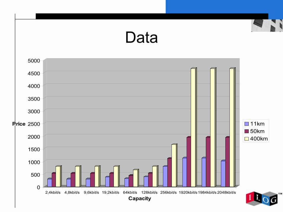
Data
0
500
1000
1500
2000
2500
3000
3500
4000
4500
5000
Price
2,4kbit/s 4,8kbit/s 9,6kbit/s 19,2kbit/s 64kbit/s 128kbit/s 256kbit/s 1920kbit/s1984kbit/s 2048kbit/s
Capacity
11km50km400km

93
Optional Constraints
❏ Security: some commodities to be secured cannot go through unsecured nodes and links
❏ No line multiplication: at most one line per arc.❏ Symmetric routing: demands from node p to node q and demands from node q
to node p are routed on symmetric paths.❏ Number of bounds (hops): the number of arcs of the path used to route a
given demand is limited.❏ Number of ports: the number of links entering into or leaving from a node is
limited.
❏ Maximal traffic: the total traffic managed by a given node is limited.
64Kb/s
64Kb/s
64Kb/s
64Kb/s

94
Numerical Characteristics

95
Mixed Integer Programming

96
Constraint Programming
❏ Routing variables: paths (D set variables)❍ A set of arcs joining the origin to the destination of the
demand❍ Basic functions : impose or forbid an arc (or a node)
❏ Dimensioning variables: chosen capacity levels (M enumerated variables)
❏ Specific constraints and constraint propagation algorithms
97
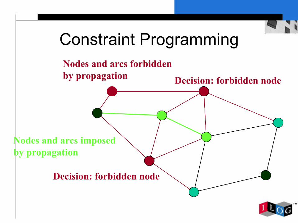
Constraint Programming
Decision: forbidden node
Nodes and arcs forbiddenby propagation
Decision: forbidden node
Nodes and arcs imposedby propagation
98
Path representation in CP
❏ “Classical” model:Graph represented by the nodes:One variable per nodeValue = possible neighboor
❏ Path from s to t: alldiff on nodes.
99
Path representation in CP
s a
b c
d e
f t
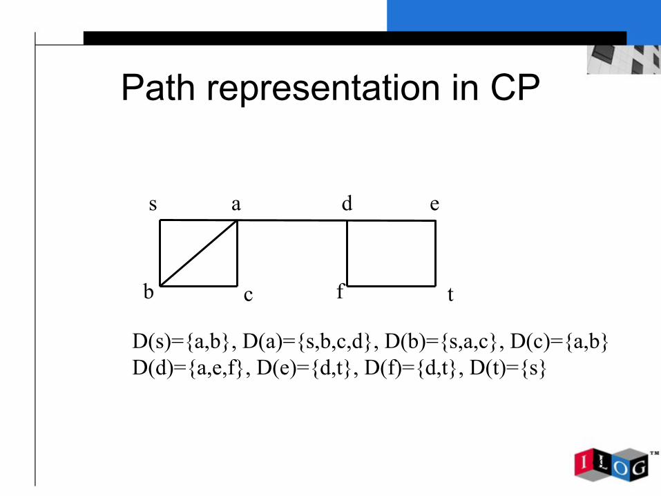
D(s)={a,b}, D(a)={s,b,c,d}, D(b)={s,a,c}, D(c)={a,b}D(d)={a,e,f}, D(e)={d,t}, D(f)={d,t}, D(t)={s}

100
Path representation in CP
s a
b c
d e
f t
D(s)={a,b}, D(a)={s,b,c,d}, D(b)={s,a,c}, D(c)={a,b}D(d)={a,e,f}, D(e)={d,t}, D(f)={d,t}, D(t)={s}

101
Path representation in CP
s a
b c
d e
f t
Problem if some variables do not belong to the path:What is the value assigned to these variables?

102
Path representation in CP
s a
b c
d e
f t
A dummy value is added to each domain: BAD IDEAD(s)={a}, D(a)={c}, D(c)={b}, D(b)={dummyb},D(d)={e}, D(e)={t}, D(f)={dummyf}, D(t)={s}
103
Path representation in CP
s a
b c
d e
f t
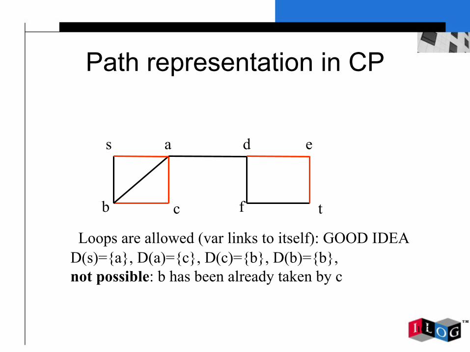
Loops are allowed (var links to itself): GOOD IDEAD(s)={a}, D(a)={c}, D(c)={b}, D(b)={b},not possible: b has been already taken by c

104
Path representation in CP
❏ “Classical” model:- One var per node- Alldiff constraint: cost for the matching: O(m) per modification

105
Rococo in CP
❏ Manipulate only graph abstractions❍ Nodes❍ Valued links❍ Shortest paths …
ILOG Solver
Rococo Program
Optimized graph API

106
New model:
❏ General point of view: we search for a subgraph. Two entities:- Digraph class - DigraphVar class
❏ A DigraphVar is a subgraph of a digraph w.r.t. properties, for instance: path.It is defined from a Digraph
❏

107
New model:
❏ General point of view: we search for a subgraph. Two entities:- Digraph class - DigraphVar class
❏ A DigraphVar is a subgraph of a digraph w.r.t. properties, for instance: path.It is defined from a Digraph
❏ API similar to setvar API

108
Digraph
❏ class IlcDigraph {IlcDigraph(IlcInt nbNodes,IlcIntArray from,IlcIntArray to);IlcInt getNbNodes()const;IlcInt getNbArcs()const;IlcInt getNbOutgoingArcs(const IlcInt node) const;IlcInt getNbIncomingArcs(const IlcInt node) const;IlcInt getEmanatingNode(const IlcInt arc)const;IlcInt getTerminatingNode(const IlcInt arc)const;IlcInt getFirstOutgoingArc(const IlcInt node)const;IlcInt getNextOutgoingArc(const IlcInt node, const IlcInt arc)const;IlcInt getFirstIncomingArc(const IlcInt node)const;IlcInt getNextIncomingArc(const IlcInt node, const IlcInt arc)const;
109
Digraph Variable
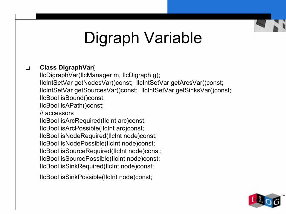
❏ Class DigraphVar{IlcDigraphVar(IlcManager m, IlcDigraph g);IlcIntSetVar getNodesVar()const; IlcIntSetVar getArcsVar()const;IlcIntSetVar getSourcesVar()const; IlcIntSetVar getSinksVar()const;IlcBool isBound()const;IlcBool isAPath()const; // accessors IlcBool isArcRequired(IlcInt arc)const; IlcBool isArcPossible(IlcInt arc)const; IlcBool isNodeRequired(IlcInt node)const; IlcBool isNodePossible(IlcInt node)const; IlcBool isSourceRequired(IlcInt node)const; IlcBool isSourcePossible(IlcInt node)const; IlcBool isSinkRequired(IlcInt node)const;
IlcBool isSinkPossible(IlcInt node)const;
110
Digraph Variable
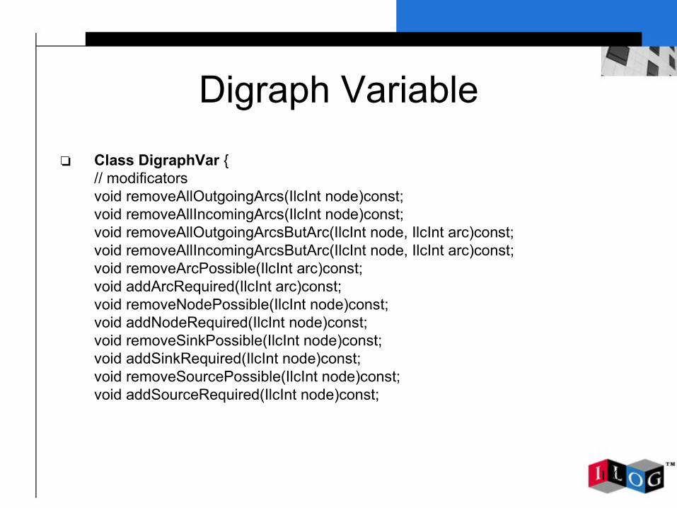
❏ Class DigraphVar {// modificators void removeAllOutgoingArcs(IlcInt node)const;void removeAllIncomingArcs(IlcInt node)const;void removeAllOutgoingArcsButArc(IlcInt node, IlcInt arc)const;void removeAllIncomingArcsButArc(IlcInt node, IlcInt arc)const;void removeArcPossible(IlcInt arc)const; void addArcRequired(IlcInt arc)const;void removeNodePossible(IlcInt node)const;void addNodeRequired(IlcInt node)const; void removeSinkPossible(IlcInt node)const; void addSinkRequired(IlcInt node)const;void removeSourcePossible(IlcInt node)const;void addSourceRequired(IlcInt node)const;
111
Digraph Variable
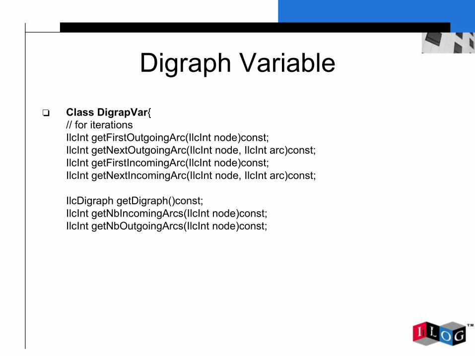
❏ Class DigrapVar{// for iterationsIlcInt getFirstOutgoingArc(IlcInt node)const;IlcInt getNextOutgoingArc(IlcInt node, IlcInt arc)const;IlcInt getFirstIncomingArc(IlcInt node)const;IlcInt getNextIncomingArc(IlcInt node, IlcInt arc)const;
IlcDigraph getDigraph()const;IlcInt getNbIncomingArcs(IlcInt node)const;IlcInt getNbOutgoingArcs(IlcInt node)const;

112
Digraph Variable
❏ Class DigraphVar{// graph functionsIlcInt getFirstArcPossibleOnShortestPath(IlcIntDistanceFunctionI* d,
const IlcInt source, const IlcInt sink,IlcInt dem=1)const;
IlcInt computeShortestPathDistance(IlcIntDistanceFunctionI* dist, const IlcInt source,
const IlcInt sink, IlcInt dem=1)const;
IlcIntArray computeShortestPath(IlcIntDistanceFunctionI* dist, const IlcInt source,
const IlcInt sink, IlcInt dem=1)const;
113
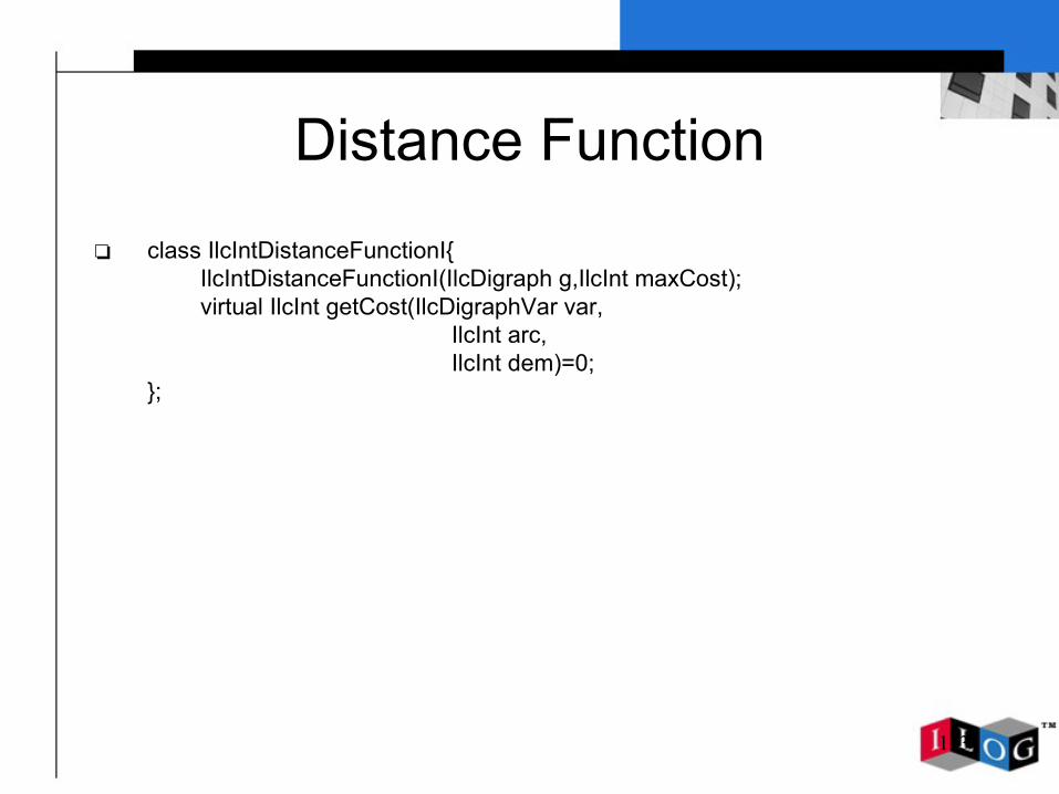
Distance Function
❏ class IlcIntDistanceFunctionI{IlcIntDistanceFunctionI(IlcDigraph g,IlcInt maxCost);
virtual IlcInt getCost(IlcDigraphVar var, IlcInt arc, IlcInt dem)=0;
};
114
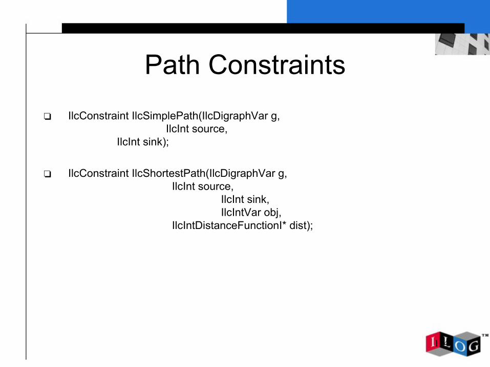
Path Constraints
❏ IlcConstraint IlcSimplePath(IlcDigraphVar g, IlcInt source, IlcInt sink);
❏ IlcConstraint IlcShortestPath(IlcDigraphVar g, IlcInt source,
IlcInt sink, IlcIntVar obj,
IlcIntDistanceFunctionI* dist);
115
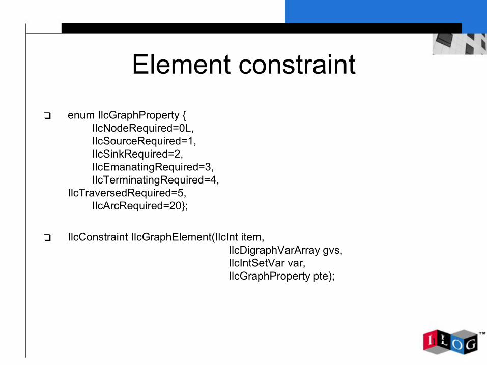
Element constraint
❏ enum IlcGraphProperty {IlcNodeRequired=0L, IlcSourceRequired=1, IlcSinkRequired=2, IlcEmanatingRequired=3, IlcTerminatingRequired=4,
IlcTraversedRequired=5, IlcArcRequired=20};
❏ IlcConstraint IlcGraphElement(IlcInt item, IlcDigraphVarArray gvs,
IlcIntSetVar var, IlcGraphProperty pte);

116
Selectors
❏ class IlcDigraphSelectDigraphVarI {IlcDigraphSelectDigraphVarI(){}virtual IlcInt select(IlcDigraphVarArray vars)=0;
};
❏ class IlcDigraphSelectArcI {IlcDigraphSelectArcI(){}virtual IlcInt select(IlcDigraphVarArray vars, IlcInt index)=0;
};
117
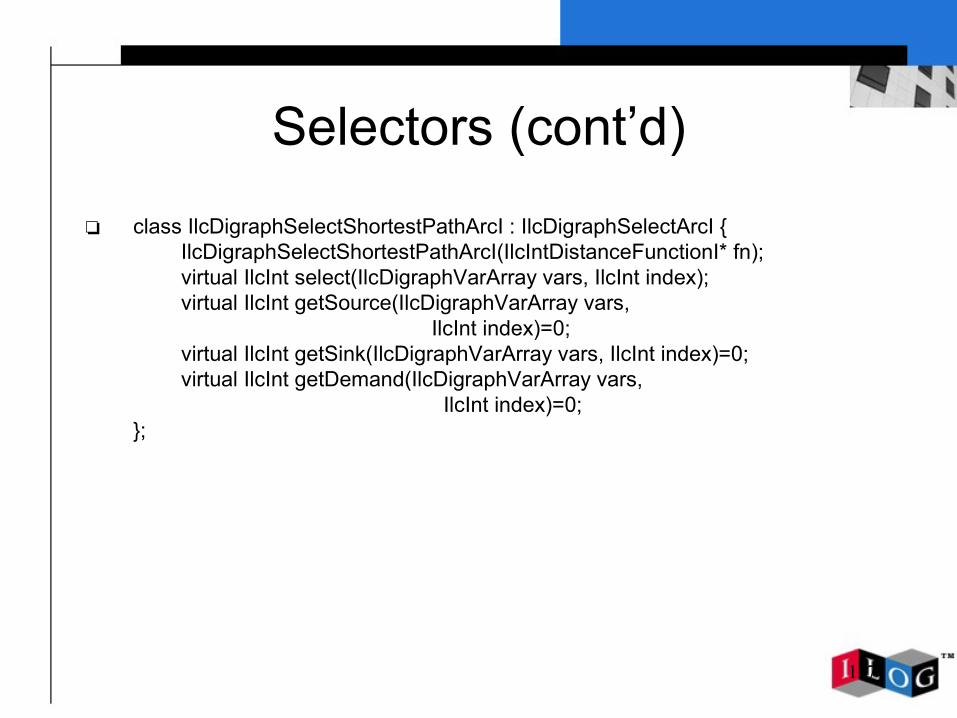
Selectors (cont’d)
❏ class IlcDigraphSelectShortestPathArcI : IlcDigraphSelectArcI {IlcDigraphSelectShortestPathArcI(IlcIntDistanceFunctionI* fn);virtual IlcInt select(IlcDigraphVarArray vars, IlcInt index);virtual IlcInt getSource(IlcDigraphVarArray vars,
IlcInt index)=0;virtual IlcInt getSink(IlcDigraphVarArray vars, IlcInt index)=0;virtual IlcInt getDemand(IlcDigraphVarArray vars,
IlcInt index)=0;};

118
Goals
❏ IlcGoal IlcDigraphRequireArc(IlcManager m, IlcDigraphVar digraph,
IlcInt arcIndex);
❏ IlcGoal IlcDigraphRemoveArc(IlcManager m, IlcDigraphVar digraph, IlcInt arcIndex);
❏ IlcGoal IlcDigraphAddArc(IlcManager m, IlcDigraphVarArray vars,
IlcInt index, IlcDigraphSelectArcI* selectArc);

119
Goals (cont’d)
❏ IlcGoal IlcDigraphInstantiate(IlcManager m, IlcDigraphVarArray vars,
IlcInt index, IlcDigraphSelectArcI* selectArc);
❏ IlcGoal IlcDigraphGenerate(IlcManager m, IlcDigraphVarArray vars, IlcDigraphSelectDigraphVarI* selectD,
IlcDigraphSelectArcI* selectArc);
120
Why not PathVar?
❏ Path is a property of a graph. We prefer to express properties by constraint
❏ In any cases, we need to be able to test if an object is a path/tree/cycle …

121
Rococo in CP
❏ Advantages of digraph variables:❍ Simple❍ Open to many additional constraints❍ Much more efficient than basic constraint programming
(combines constraint programming with optimization algorithms on graphs)

122
Rococo in CP
❏ Search strategy: select the most important demand and the path for which the additional (marginal) cost for routing this demand is minimal
❍ Shortest path problem with constraints❍ Successive constraints: impose the last arc, then the previous
arc, ..., and finally the first arc of the shortest path❍ Each of these added constraints leads to creating a choice point:
upon backtracking, the imposed arc is forbidden and a new shortest path, taking this interdiction into account, computed

123
Improvements of CP
❏ Direct constraint between variables representing the paths and variables representing the traffic through each node
❏ Use of Parallel Solver❍ A few lines of code
❏ Modification of the tree-search traversal strategy❍ Branch more close to the root of the tree
124
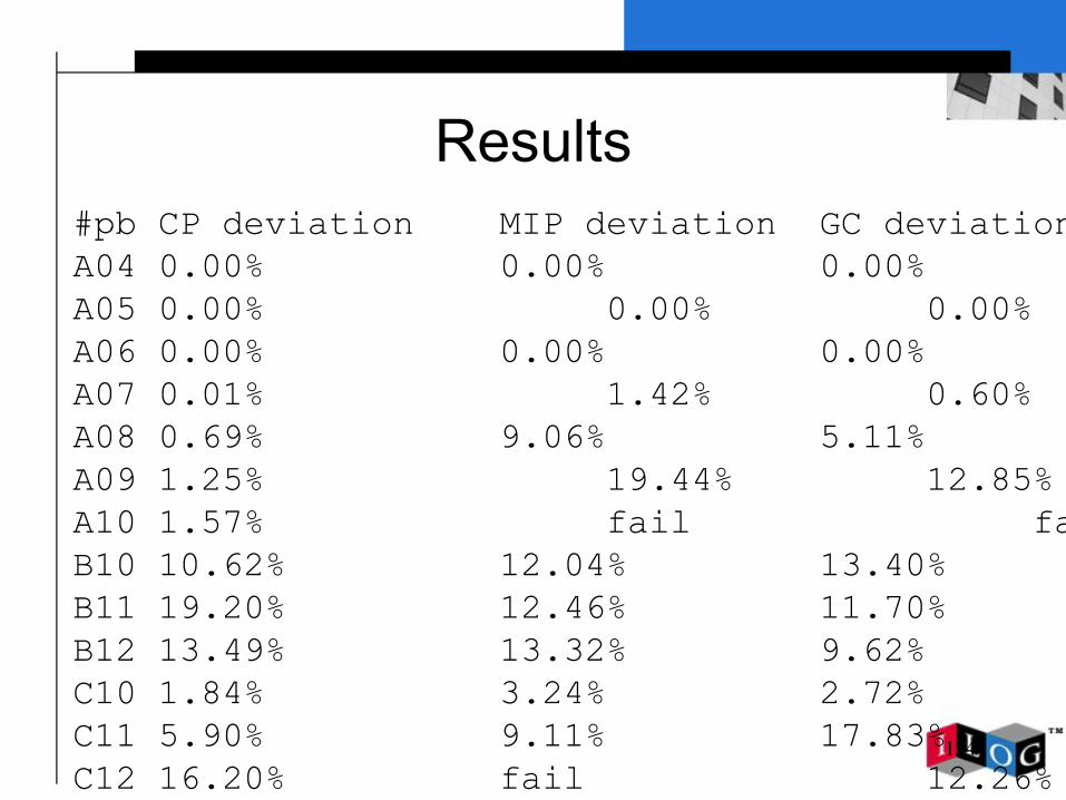
Results#pb CP deviation MIP deviation GC deviationA04 0.00% 0.00% 0.00%A05 0.00% 0.00% 0.00%A06 0.00% 0.00% 0.00%A07 0.01% 1.42% 0.60%A08 0.69% 9.06% 5.11%A09 1.25% 19.44% 12.85%A10 1.57% fail fail B10 10.62% 12.04% 13.40%B11 19.20% 12.46% 11.70%B12 13.49% 13.32% 9.62%C10 1.84% 3.24% 2.72%C11 5.90% 9.11% 17.83%C12 16.20% fail 12.26%

125
Results
❏ France Telecom considers that CP gives the most interesting result.
❏ CP approach has been optimized mainly for A series.
❏ A lot of work could be done for the other series❏ Result of Column Generation comes from a PhD
thesis (A. Chabrier) mainly dedicated to this problem
126
Pros and Cons of Different Techniques (1)
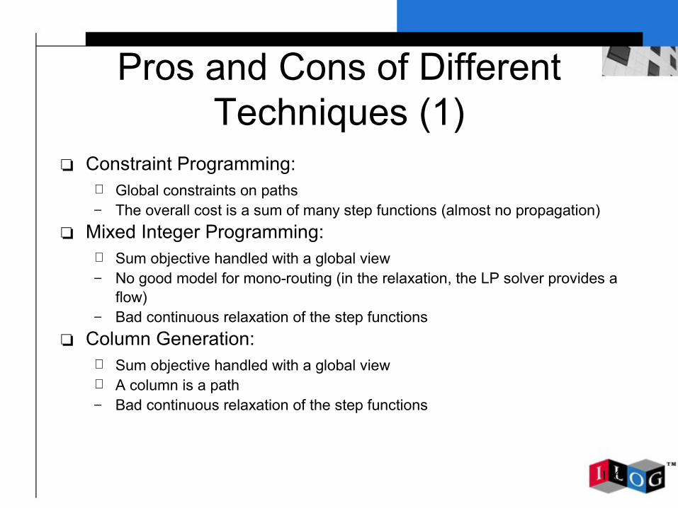
❏ Constraint Programming:+ Global constraints on paths– The overall cost is a sum of many step functions (almost no propagation)
❏ Mixed Integer Programming:+ Sum objective handled with a global view– No good model for mono-routing (in the relaxation, the LP solver provides a
flow)– Bad continuous relaxation of the step functions
❏ Column Generation:+ Sum objective handled with a global view+ A column is a path– Bad continuous relaxation of the step functions
127
Pros and Cons of Different Techniques (2)
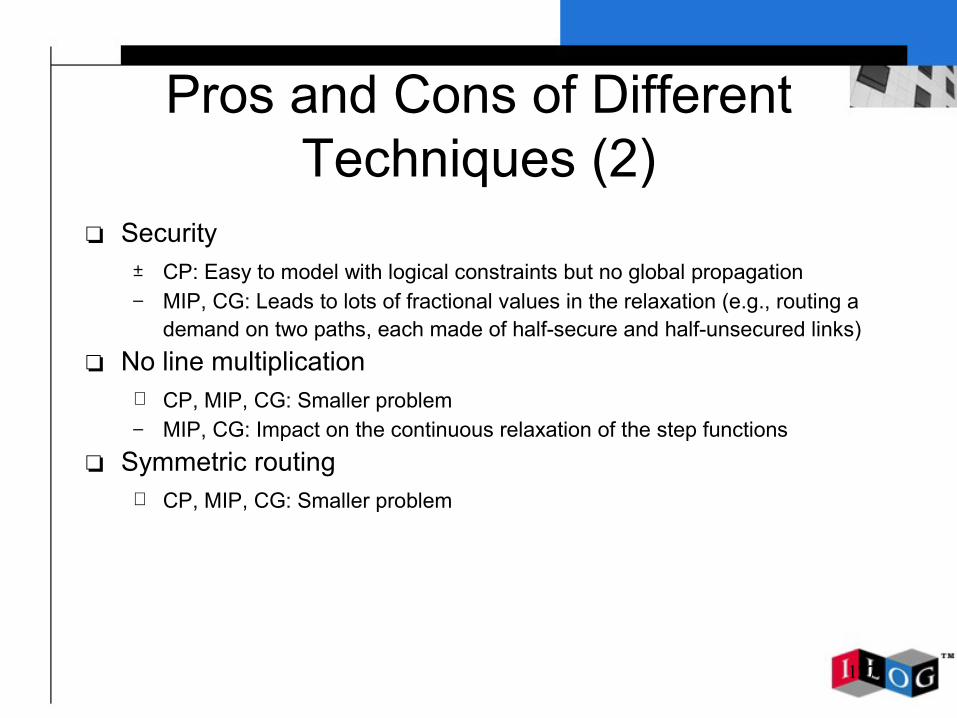
❏ Security± CP: Easy to model with logical constraints but no global propagation– MIP, CG: Leads to lots of fractional values in the relaxation (e.g., routing a
demand on two paths, each made of half-secure and half-unsecured links)❏ No line multiplication
+ CP, MIP, CG: Smaller problem– MIP, CG: Impact on the continuous relaxation of the step functions
❏ Symmetric routing+ CP, MIP, CG: Smaller problem
128
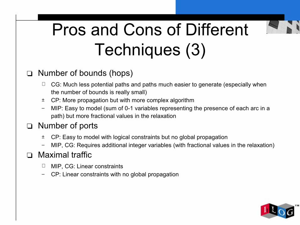
Pros and Cons of Different Techniques (3)
❏ Number of bounds (hops)+ CG: Much less potential paths and paths much easier to generate (especially when
the number of bounds is really small)± CP: More propagation but with more complex algorithm– MIP: Easy to model (sum of 0-1 variables representing the presence of each arc in a
path) but more fractional values in the relaxation
❏ Number of ports± CP: Easy to model with logical constraints but no global propagation– MIP, CG: Requires additional integer variables (with fractional values in the relaxation)
❏ Maximal traffic+ MIP, CG: Linear constraints– CP: Linear constraints with no global propagation
129
Plan
❏ Principles of Constraint Programming❏ A rostering problem ❏ Modeling in CP: Principles❏ A difficult problem❏ A Network Design problem❏ Modeling Over-constrained problems❏ Discussion❏ Conclusion

130
Over Constrained ProblemsOver Constrained Problems
❏ No solution satisfies all the constraints❏ What can we do?❏ Some constraints have to be relaxed
❍ Hard constraints: must be satisfied❍ Soft constraints: can be relaxed

131
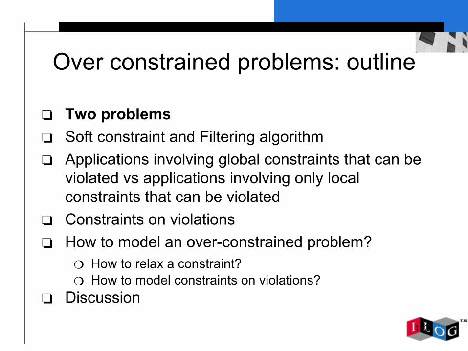
Over constrained problems: outline
❏ Two problems❏ Soft constraint and Filtering algorithm❏ Applications involving global constraints that can be
violated vs applications involving only local constraints that can be violated
❏ Constraints on violations❏ How to model an over-constrained problem?
❍ How to relax a constraint?❍ How to model constraints on violations?
❏ Discussion
132
Over constrained problems: outline
❏ Two problems❏ Soft constraint and Filtering algorithm❏ Applications involving global constraints that can be
violated vs applications involving only local constraints that can be violated
❏ Constraints on violations❏ How to model an over-constrained problem?
❍ How to relax a constraint?❍ How to model constraints on violations?
❏ Discussion
133
Car sequencing
❏ Problem : computes the sequencing order of cars that will be built on an assembly line
❏ Many different types of cars can be built on an assembly line.
❏ A car = a basic car + options (color, motor, telephone, seats, …).
❏ A car = a configuration of options
134
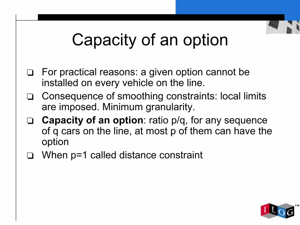
Capacity of an option
❏ For practical reasons: a given option cannot be installed on every vehicle on the line.
❏ Consequence of smoothing constraints: local limits are imposed. Minimum granularity.
❏ Capacity of an option: ratio p/q, for any sequence of q cars on the line, at most p of them can have the option
❏ When p=1 called distance constraint
135
Car sequencing
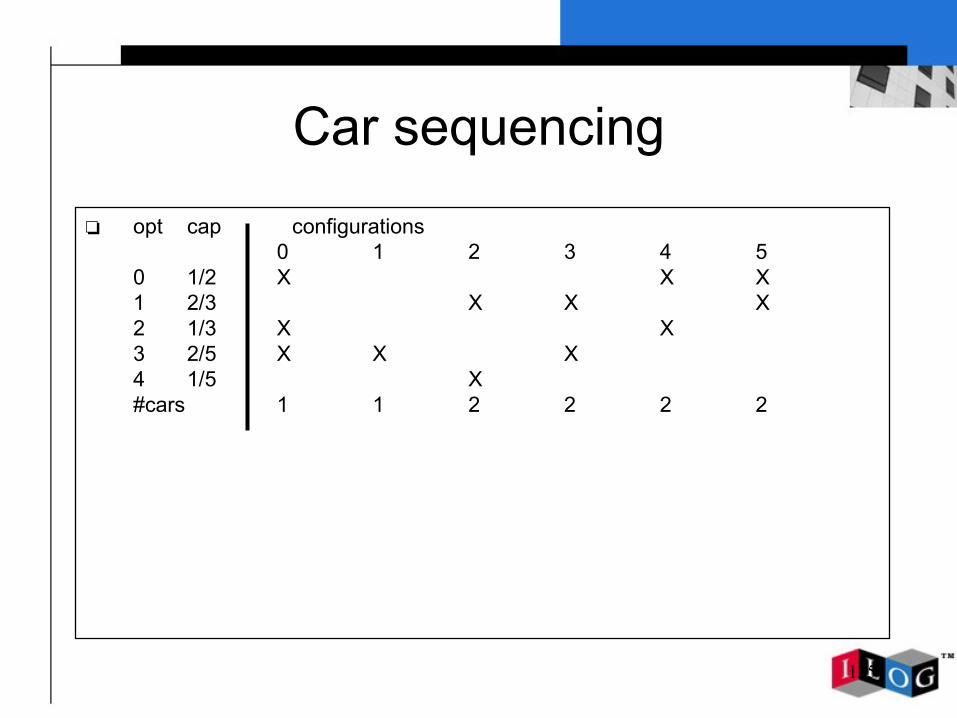
❏ opt cap configurations0 1 2 3 4 5
0 1/2 X X X1 2/3 X X X2 1/3 X X3 2/5 X X X4 1/5 X#cars 1 1 2 2 2 2
136
Car sequencing
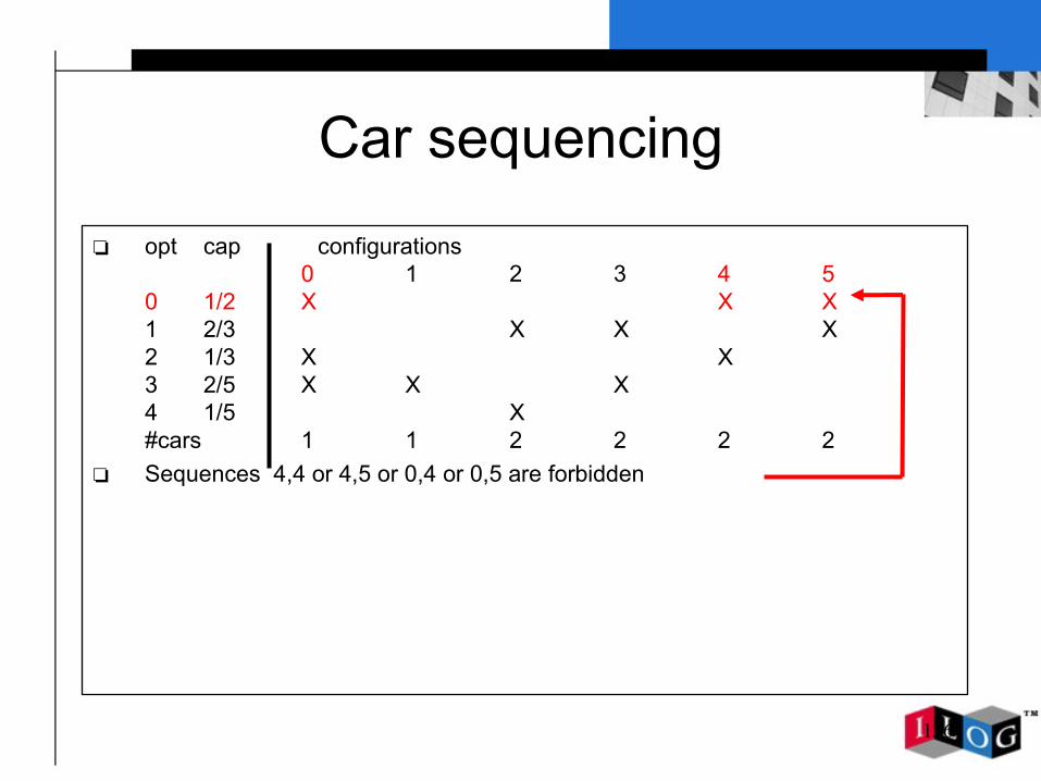
❏ opt cap configurations0 1 2 3 4 5
0 1/2 X X X1 2/3 X X X2 1/3 X X3 2/5 X X X4 1/5 X#cars 1 1 2 2 2 2
❏ Sequences 4,4 or 4,5 or 0,4 or 0,5 are forbidden
137
Car sequencing
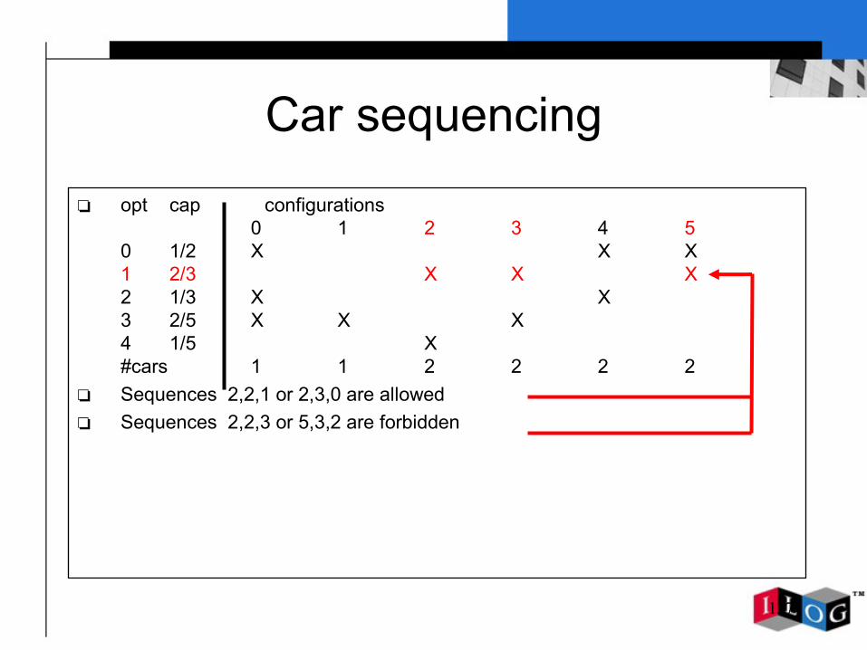
❏ opt cap configurations0 1 2 3 4 5
0 1/2 X X X1 2/3 X X X2 1/3 X X3 2/5 X X X4 1/5 X#cars 1 1 2 2 2 2
❏ Sequences 2,2,1 or 2,3,0 are allowed❏ Sequences 2,2,3 or 5,3,2 are forbidden
138
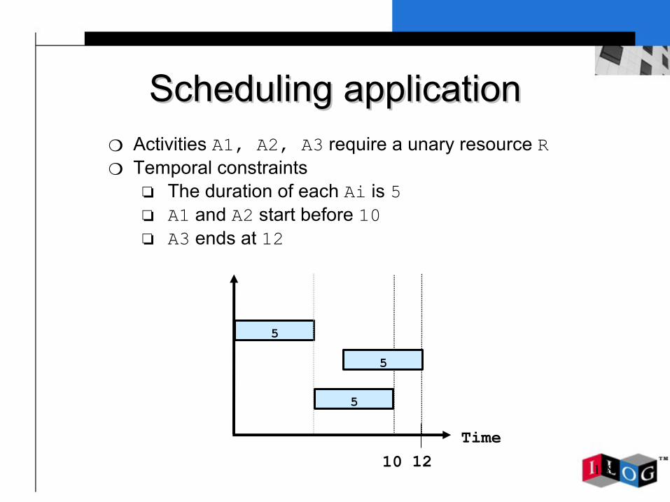
Scheduling applicationScheduling application❍ Activities A1, A2, A3 require a unary resource R❍ Temporal constraints
❏ The duration of each Ai is 5❏ A1 and A2 start before 10❏ A3 ends at 12
1210Time
55
5

139
Over constrained problems: outline
❏ Two problems❏ Soft constraint and Filtering algorithm❏ Applications involving global constraints that can be
violated vs applications involving only local constraints that can be violated
❏ Constraints on violations❏ How to model an over-constrained problem?
❍ How to relax a constraint?❍ How to model constraints on violations?
❏ Discussion

140
Soft constraint
❏ A soft constraint is a constraint that can be violated❏ The violation can be associated with a cost that can
be:❍ The same for any violation❍ Depends on the violation
❏ Example: x < y, if x ≥ y we can have❍ A fixed cost: cost = c❍ A cost depending on the violation: cost = x –y or
cost = (x-y)2

141
Soft constraint and Filtering algorithm
❏ When the violation is accepted this means that we accept that any combination of values satisfies the constraint.
142
Soft constraint and Filtering algorithm
❏ When the violation is accepted this means that we accept that any combination of values satisfies the constraint.
❏ Roughly, the constraint become an universal constraint associating a cost with any tuple, so we loose the structure of the constraint
143
Soft constraint and Filtering algorithm
❏ When the violation is accepted this means that we accept that any combination of values satisfies the constraint.
❏ Roughly, the constraint become an universal constraint associating a cost with any tuple, so we loose the structure of the constraint
❏ Problem with filtering algorithm (FA): ❍ FA exploits the structure of the constraints❍ FA are not efficient when everything is possible!
144
Soft constraint and Filtering algorithm
❏ When the violation is accepted this means that we accept that any combination of values satisfies the constraint.
❏ Roughly, the constraint become an universal constraint associating a cost with any tuple, so we loose the structure of the constraint
❏ Problem with filtering algorithm (FA): ❍ FA exploits the structure of the constraints❍ FA are not efficient when everything is possible!
❏ Filtering for soft depends mainly on back propagation. Problem with global constraints

145
Over constrained problems: outline
❏ Two problems❏ Soft constraint and Filtering algorithm❏ Applications involving global constraints that
can be violated vs applications involving only local constraints that can be violated
❏ Constraints on violations❏ How to model an over-constrained problem?
❍ How to relax a constraint?❍ How to model constraints on violations?
❏ Discussion
146
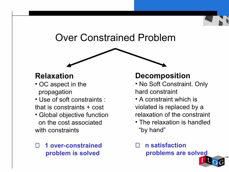
Over Constrained Problem
Relaxation• OC aspect in the propagation• Use of soft constraints : that is constraints + cost• Global objective function on the cost associated with constraints
⇒ 1 over-constrained problem is solved
Decomposition• No Soft Constraint. Only hard constraint• A constraint which is violated is replaced by a relaxation of the constraint • The relaxation is handled “by hand”
⇒ n satisfaction problems are solved
147
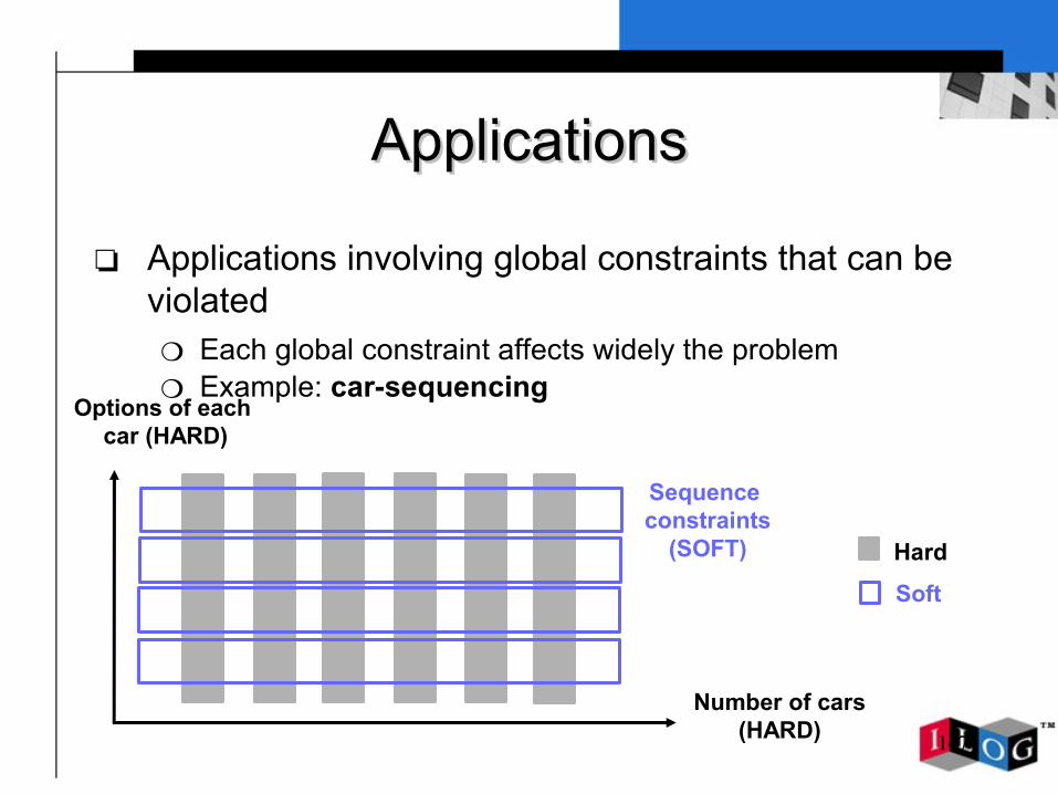
ApplicationsApplications
❏ Applications involving global constraints that can be violated❍ Each global constraint affects widely the problem❍ Example: car-sequencing
Number of cars(HARD)
Options of each car (HARD)
Sequence constraints
(SOFT) Hard
Soft

148
ApplicationsApplications
❏ Applications involving “global” soft constraints⇒ Difficult to solve with a pure relaxation approach ⇒ Decomposition methods are more adapted

149
ApplicationsApplications
❏ Applications involving “global” soft constraints⇒ Difficult to solve with a pure relaxation approach
❏ A global constraint = conjunction of constraint. Violation of a global = violation of any constraint of the conjunction
❏ The problem is not easy even with efficient global constraints, so if the global constraints are removed and replaced by a lot of constraints that can be violated then we loose the strong filtering algorithms

150
ApplicationsApplications
❏ Applications involving “global” soft constraints
⇒ Decomposition methods are more adapted❏ A succession of problems are considered. In each
problem the global constraint that are violated are relaxed by hand:❍ another global constraint replaces the previous one but it is
less constrained. For instance a p/q option will be replaced by a p+1/q option. We will manage the relaxation
❍ There is no objective, this is the user that controls the list of the problems that will be considered

151
ApplicationsApplications
❏ Application involving “Local” constraints that can be violated❍ Example: scheduling
Resources(SOFT)
Time (SOFT)
Precedence / orderconstraints
(HARD) Hard
Soft
152
ApplicationsApplications
❏ Application involving “Local” soft constraints⇒ Decomposition methods can be used⇒ Relaxation methods can be used
153
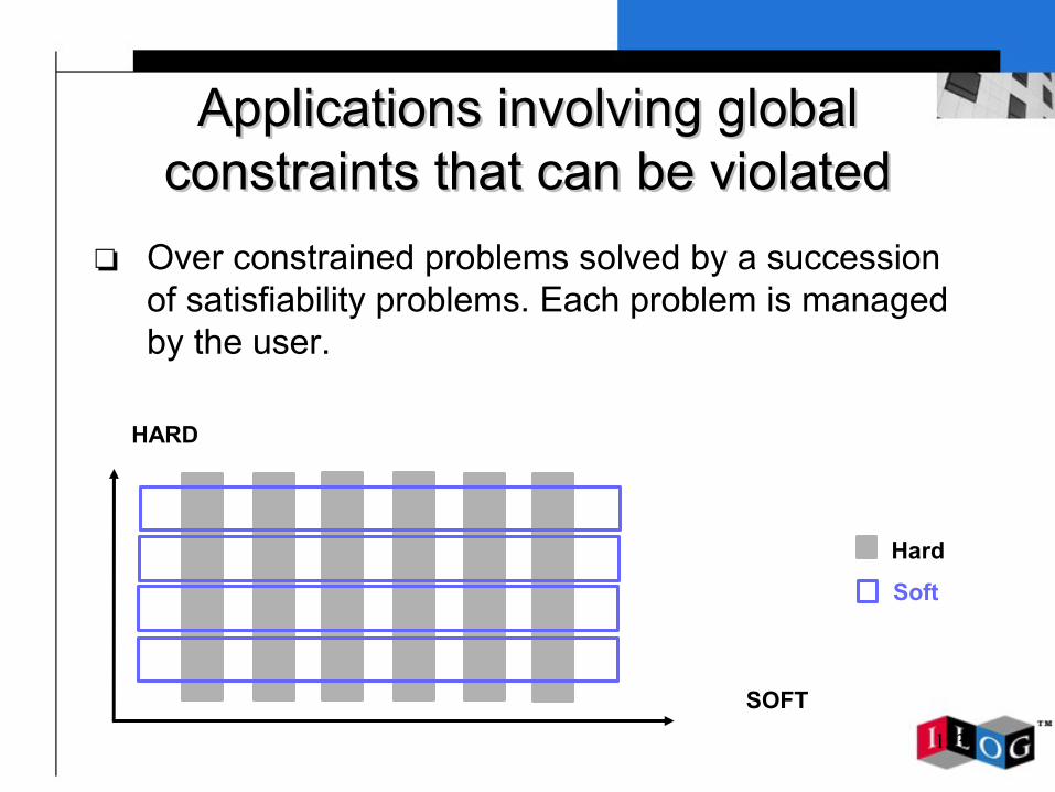
Applications involving global Applications involving global constraints that can be violatedconstraints that can be violated
❏ Over constrained problems solved by a succession of satisfiability problems. Each problem is managed by the user.
SOFT
HARD
Hard
Soft

154
Applications involving local Applications involving local constraints that can be violatedconstraints that can be violated
❏ All the constraints are relaxed (that is we accept the violation) then an optimization problem is solved. The objective is to minimize the sum of the violation costs
SOFT
HARD
Hard
Soft

155
Over constrained problems: outline
❏ Two problems❏ Soft constraint and Filtering algorithm❏ Applications involving global constraints that can be
violated vs applications involving only local constraints that can be violated
❏ Constraints on violations❏ How to model an over-constrained problem?
❍ How to relax a constraint?❍ How to model constraints on violations?
❏ Discussion

156
Constraints on violationsConstraints on violations
❏ In real world problems, the goal is much more complex than minimizing the number of constraint violations
⇒ Rules on violations❍ Distinction between hard and soft constraints❍ Priorities ❍ Control of distribution of violations in the constraint network : well
balancing of violation (homogeneity) is generally required❍ Specific dependencies between constraints
157
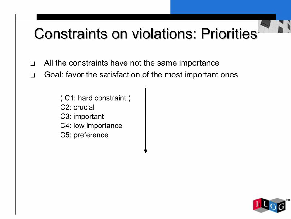
Constraints on violations: PrioritiesConstraints on violations: Priorities
❏ All the constraints have not the same importance❏ Goal: favor the satisfaction of the most important ones
( C1: hard constraint ) C2: crucial C3: important C4: low importance C5: preference

158
Well balancing of violations
❏ In many real-world applications, violations must generally be homogeneously distributed in the constraint network
❏ More complex rules with respect to distribution of violations are sometimes required
159
Well balancing of violationsWell balancing of violations
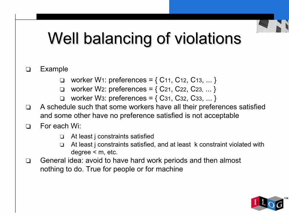
❏ Example ❏ worker W1: preferences = { C11, C12, C13, ... }❏ worker W2: preferences = { C21, C22, C23, ... }❏ worker W3: preferences = { C31, C32, C33, ... }
❏ A schedule such that some workers have all their preferences satisfied and some other have no preference satisfied is not acceptable
❏ For each Wi:❏ At least j constraints satisfied❏ At least j constraints satisfied, and at least k constraint violated with
degree < m, etc.❏ General idea: avoid to have hard work periods and then almost
nothing to do. True for people or for machine
160
Constraints on violations: Constraints on violations: DependenciesDependencies
❏ Expressing specific dependencies is generally required❏ Example
❏ « if C1 and C2 are violated then C3 must be satisfied »
161
Over constrained problems: outline
❏ Two problems❏ Soft constraint and Filtering algorithm❏ Applications involving global constraints that can be
violated vs applications involving only local constraints that can be violated
❏ Constraints on violations❏ How to model an over-constrained problem?
❍ How to relax a constraint?❍ How to model constraints on violations?
❏ Discussion

162
How to model over-constrained problems?
❏ How to relax a constraint?❏ How to model usual constraints on violations
163
How to relax a constraint?
❏ Try to keep some structure in order to have efficient filtering algorithm
❏ Use meta constraints
164
Meta Constraint
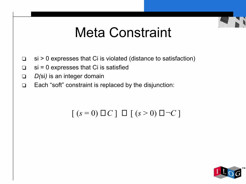
❏ si > 0 expresses that Ci is violated (distance to satisfaction)❏ si = 0 expresses that Ci is satisfied ❏ D(si) is an integer domain❏ Each “soft” constraint is replaced by the disjunction:
[ (s = 0) ∧ C ] ∨ [ (s > 0) ∧ ¬C ]
165
Meta ConstraintMeta Constraint
❏ Since valuations are expressed trough variables, constraints on these variables can be added in order to express “global rules” on violations

166
Max-SAT = Satisfiability Sum Max-SAT = Satisfiability Sum ConstraintConstraint
❏ In the ssc, each constraint Ci is replaced by:
❏ A variable unsat is used to express the objective:
[ (Ci ∧ (ui = 0)) ∨ (¬Ci ∧ (ui = 1)) ]
∑ ui i=1
# Ci
[ unsat = ]
167
Advantages of This ModelAdvantages of This Model
❏ Classical constraint optimization problem● Direct integration into a solver● Any search algorithm can be used, not only a Branch
and Bound based one. ❏ When a value is assigned to ui ∈ U, the filtering
algorithm associated with Ci (resp. ¬Ci) can be used❏ No hypothesis is made on constraints (arity)
168
Advantages of This ModelAdvantages of This Model
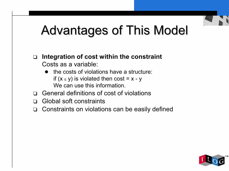
❏ Integration of cost within the constraintCosts as a variable:
● the costs of violations have a structure:if (x ≤ y) is violated then cost = x - yWe can use this information.
❏ General definitions of cost of violations❏ Global soft constraints❏ Constraints on violations can be easily defined
169
Use of the structure of the violation:Use of the structure of the violation:x x ≤≤ y y
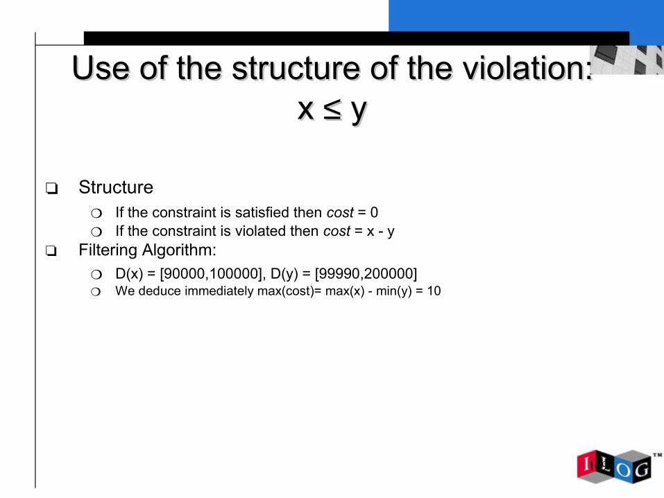
❏ Structure❍ If the constraint is satisfied then cost = 0❍ If the constraint is violated then cost = x - y
❏ Filtering Algorithm:❍ D(x) = [90000,100000], D(y) = [99990,200000]❍ We deduce immediately max(cost)= max(x) - min(y) = 10

170
General definition of the cost of violation
❏ Two different general costs:❍ Variables based violation cost❍ Primal Graph Based violation cost
❏ Some others see papers at CP-AI-OR’04 (Beldiceanu and Petit) and papers at workshop on soft constraints at CP’04.

171
Variable based violation cost
❏ How many variables must be removed to satisfy the constraint?
❏ Alldiff({x1,x2,x3,x4,x5})(a,a,a,b,b) cost = 3(a,a,a,a,b) cost = 3
172
Primal graph based partition cost
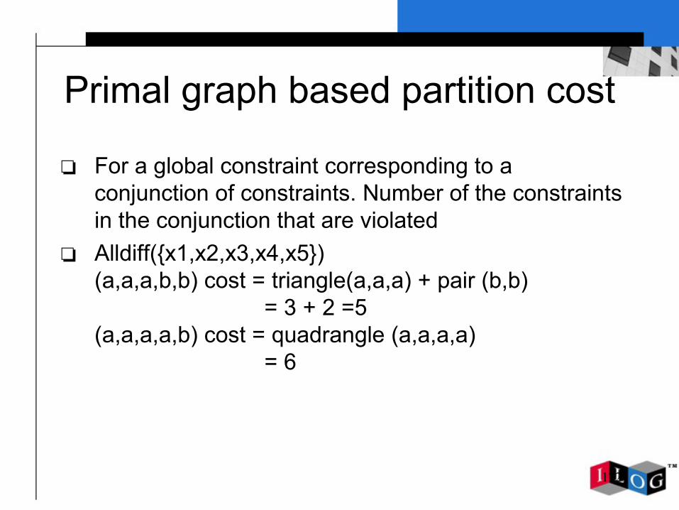
❏ For a global constraint corresponding to a conjunction of constraints. Number of the constraints in the conjunction that are violated
❏ Alldiff({x1,x2,x3,x4,x5})(a,a,a,b,b) cost = triangle(a,a,a) + pair (b,b)
= 3 + 2 =5(a,a,a,a,b) cost = quadrangle (a,a,a,a)
= 6
173
All Different constraintAll Different constraint
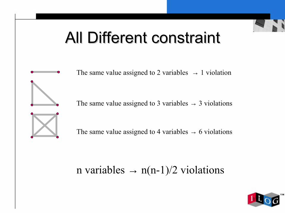
The same value assigned to 2 variables → 1 violation
The same value assigned to 3 variables → 3 violations
The same value assigned to 4 variables → 6 violations
n variables → n(n-1)/2 violations
174
Meta-constraints for Expressing Meta-constraints for Expressing HomogeneityHomogeneity
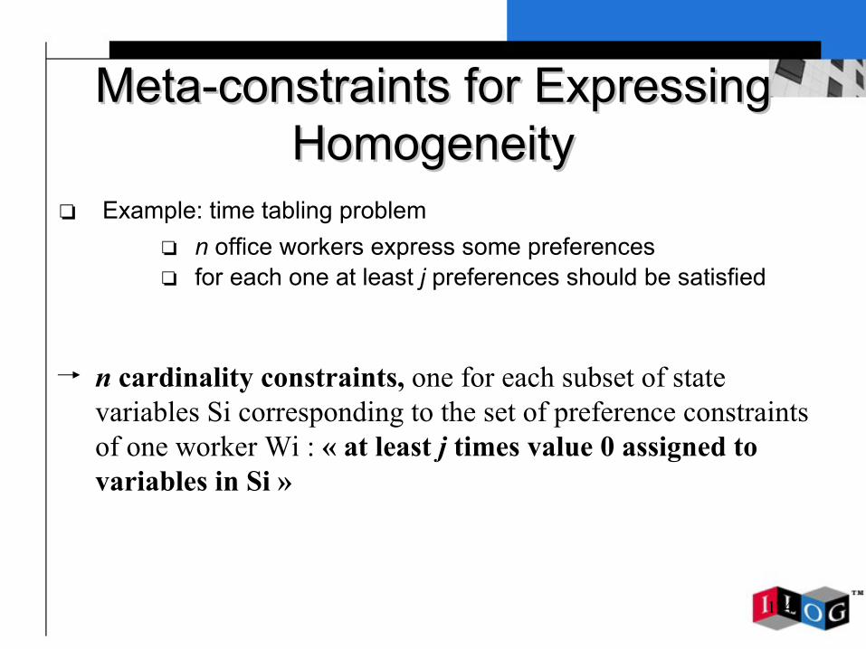
❏ Example: time tabling problem❏ n office workers express some preferences❏ for each one at least j preferences should be satisfied
n cardinality constraints, one for each subset of state variables Si corresponding to the set of preference constraints of one worker Wi : « at least j times value 0 assigned to variables in Si »
175
Meta-constraints for Expressing Meta-constraints for Expressing DependenciesDependencies
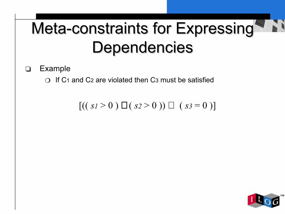
❏ Example❍ If C1 and C2 are violated then C3 must be satisfied
[(( s1 > 0 ) ∧ ( s2 > 0 )) ⇒ ( s3 = 0 )]

176
Over constrained problems: outline
❏ Two problems❏ Soft constraint and Filtering algorithm❏ Applications involving global constraints that can be
violated vs applications involving only local constraints that can be violated
❏ Constraints on violations❏ How to model an over-constrained problem?
❍ How to relax a constraint?❍ How to model constraints on violations?
❏ Discussion

177
Discussion
❏ Well balancing of violations can be difficult to express.
❏ Real life example: Capacity constraints (smoothing constraints are soft): p/q.
❍ Violation: (p’-p)2/q2, then minimization of the variance.❍ Signification: consider 1/5 and ½,
❏ a violation of 1 is less important for 1/5 than for 1/2, so q2 is considered
❏ two violations of 1 are less important than one violation of 2, so (p’-p)2 is considered
❍ Difficult to model
178
Discussion
❏ A quite interesting approach has been proposed by L. Perron and P. Shaw (see in their CP’04 paper) for car sequencing
❏ 100 cars to schedule with a book order of 100 cars. Accept to have dummy cars (perfect cars), that is extend the book order -> 110 cars
❏ Then try to minimize the number of perfect cars❏ Then replace perfect cars by real cars❏ Seems very interesting because the model of the
initial problems is not change at all and we work only with hard constraints

179
Meta constraints vs other models
❏ Valued CSP is not able to take into account the structure of the violated constraints
❏ Valued CSP contains no back propagation because the cost is not a variable
❏ Valued CSP are not able to manage constraints on violation
❏ If we represent constraints on violations by constraints we do not need to invent a new XXX Csp for every constraint on violations
180
Plan
❏ Principles of Constraint Programming❏ A rostering problem ❏ Modeling in CP: Principles❏ A difficult problem❏ A Network Design problem❏ Modeling Over-constrained problems❏ Discussion❏ Conclusion
181
Hard problem
❏ Consider a problem P that you are unable to solve. How can you improve the resolution?

182
Hard problem
❏ Consider a problem P that you are unable to solve. How can you improve the resolution?
❏ By identifying hard sub-problems H of P
183
Hard problem
❏ Consider a problem P that you are unable to solve. How can you improve the resolution?
❏ By identifying hard sub-problems H of P❏ By improving the resolution of some sub-problems R
of P and by using filtering algorithm for R.
184
Problem
❏ How can we identify a sub-problem R for which we can improve its resolution?
❏ How can we write a specific filtering algorithm for this sub-problem R?
❏ This is time-consuming and not necessarily worthwhile.
185
Improving the resolution of R
❏ R can be viewed as a global constraint:An allowed tuple of this constraint is a solution of R and conversely.
❏ Consistency of the constraint = R has a solution.
186
GAC-Schema: instantiation
❏ List of allowed tuples❏ List of forbidden tuples❏ Predicates❏ Any OR algorithm❏ Solver reentrace
187
GAC-Schema
❏ Idea: tuple = solution of the constraintsupport = valid tuple- while the tuple is valid: do nothing
- if the tuple is no longer valid, then search for a new support for the values it contains
❏ a solution (support) can be computed by any OR algorithm. A solution is needed not only the fact that there is one.
188
GAC-Schema: complexity
❏ CC complexity to check consistency (seek in table, call to OR algorithm): seek for a Support costs CC
❏ n variables, d values:for each value: CCfor all values: O(ndCC)
❏ For any OR algorithm which is able to compute a solution, Arc consistency can be achieved in O(ndCC).

189
AC for R
❏ All the possible solutions of R are computed once and for all. They are saved in a database. GAC-Schema + allowed is used
❏ Only the combinations of values that are not solution are saved. GAC-Schema + forbidden
❏ Solutions are computed on the fly when we want to know if a value belongs to a current solution of R.
190
Improvement of the resolution
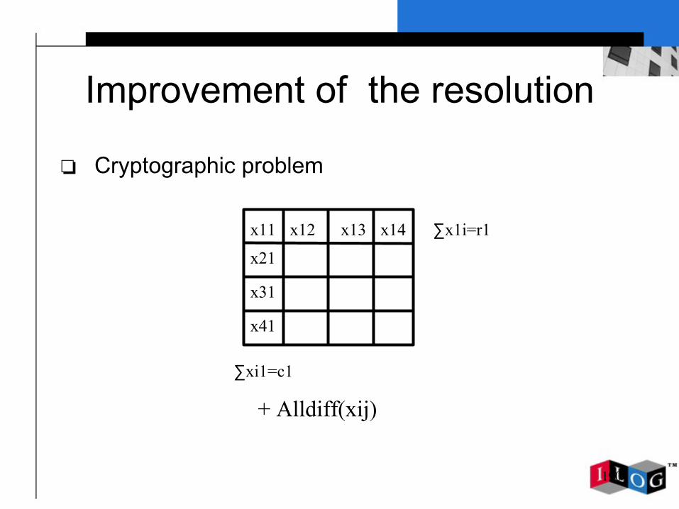
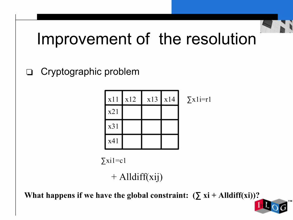
❏ Cryptographic problem
x11 x12
x21
x31
x41
x14x13 ∑x1i=r1
∑xi1=c1
+ Alldiff(xij)
191
Improvement of the resolution
❏ Cryptographic problem
x11 x12
x21
x31
x41
x14x13 ∑x1i=r1
∑xi1=c1
+ Alldiff(xij)
What happens if we have the global constraint: (∑ xi + Alldiff(xi))?

192
Improvement of the resolution
❏ Model 1: Sum for each row and each column + Alldiff(xij)
❏ Model 2: (∑ xi + Alldiff(xi)) for each row and each column + Alldiff(xij)
9,985 591 591 1.36 7.2 51 2,373 127 127 0.3 1.7 18
4 0 0 0 0.5 8.5easiestaveragehardest
model1 model2 pred
#backtracks time
5 x 5

193
Improvement of the resolution
❏ Model 1: Sum for each row and each column + Alldiff(xij)
❏ Model 2: (∑ xi + Alldiff(xi)) for each row and each column + Alldiff(xij)
1,623,557 2,598 2,598 520 42 too long75,548 281 281 26.2 6.7 too long
3 0 0 0.03 2.5 too longeasiestaveragehardest
model1 model2 pred
#backtracks time
6 x 6

194
Identification of the difficulty
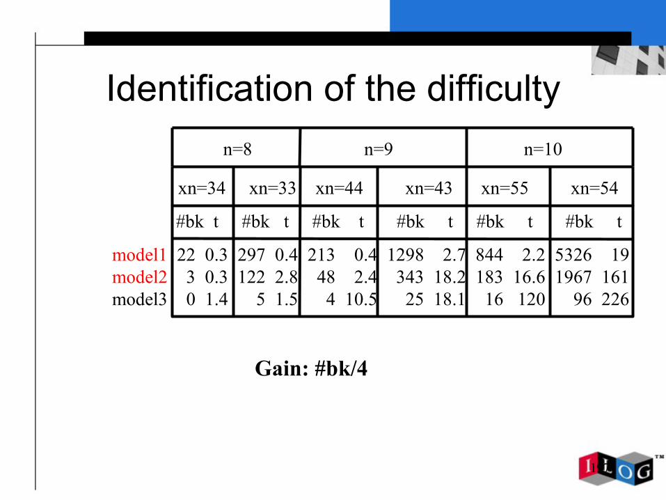
❏ Golomb ruler (see CSP lib):“A Golomb ruler may be defined as a set of n integers 0=x1 < x2 < … < xn s.t. the n(n-1)/2 differences (xj - xi) are distinct. Goal minimize xn.”
❏ with CP difficult for n > 13.

195
Identification of the difficulty
❏ Model1: x1,…,xn = variables; (xi-xj)= variables. Alldiff involving all the variables.
❏ Model2: diff1i = xi - x(i-1)Model1 + global constraint:
Sum(diff1i)=xn and Alldiff(diff1i)❏ Model3: diff2i= xi - x(i-2)
Model1 + global constraint: Sum(diff1i)=xn and Alldiff(diff1i U diff2i)

196
Identification of the difficulty
model1 22 0.3 297 0.4 213 0.4 1298 2.7 844 2.2 5326 19model2 3 0.3 122 2.8 48 2.4 343 18.2 183 16.6 1967 161model3 0 1.4 5 1.5 4 10.5 25 18.1 16 120 96 226
#bk t #bk t #bk t #bk t #bk t #bk t
xn=34 xn=33 xn=44 xn=43 xn=55 xn=54
n=8 n=9 n=10
197
Identification of the difficulty
model1 22 0.3 297 0.4 213 0.4 1298 2.7 844 2.2 5326 19model2 3 0.3 122 2.8 48 2.4 343 18.2 183 16.6 1967 161model3 0 1.4 5 1.5 4 10.5 25 18.1 16 120 96 226
#bk t #bk t #bk t #bk t #bk t #bk t
xn=34 xn=33 xn=44 xn=43 xn=55 xn=54
n=8 n=9 n=10
Gain: #bk/4

198
Identification of the difficulty
model1 22 0.3 297 0.4 213 0.4 1298 2.7 844 2.2 5326 19model2 3 0.3 122 2.8 48 2.4 343 18.2 183 16.6 1967 161model3 0 1.4 5 1.5 4 10.5 25 18.1 16 120 96 226
#bk t #bk t #bk t #bk t #bk t #bk t
xn=34 xn=33 xn=44 xn=43 xn=55 xn=54
n=8 n=9 n=10
Gain: problem almost solved!
Sum(diff1i)=xn and Alldiff(diff1i U diff2i): involves only n variables

199
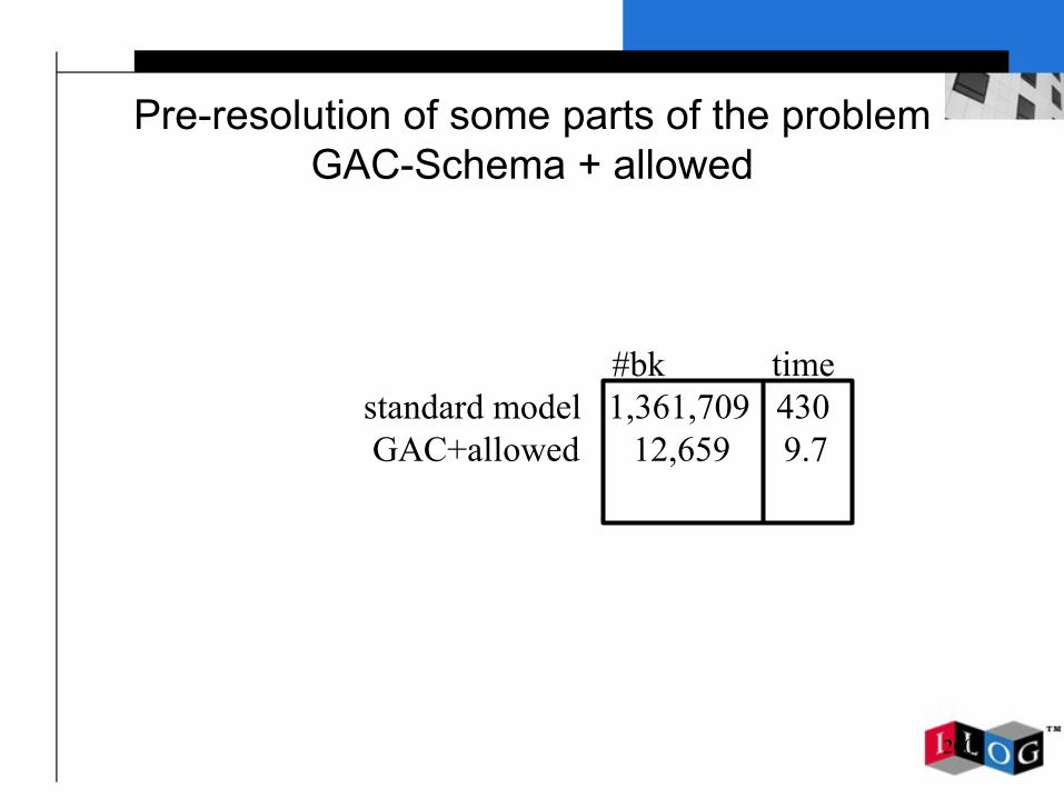
Pre-resolution of some parts of the problemGAC-Schema + allowed
❏ Configuration problem:5 types of components: {glass, plastic, steel, wood, copper}3 types of bins: {red, blue, green} whose capacity is red 5, blue 5, green 6Constraints:- red can contain glass, cooper, wood- blue can contain glass, steel, cooper- green can contain plastic, copper, wood- wood require plastic; glass exclusive copper- red contains at most 1 of wood- green contains at most 2 of woodFor all the bins there is either no plastic or at least 2 plasticGiven an initial supply of 12 of glass, 10 of plastic, 8 of steel, 12 of wood and 8 of copper; what is the minimum total number of bins?
200
Pre-resolution of some parts of the problemGAC-Schema + allowed
#bk timestandard model 1,361,709 430 GAC+allowed 12,659 9.7

201
GAC Schema + allowed
❏ It is important to be able to generate all solutions of a problem
❏ There is almost no efficient algorithms that are available
❏ Any idea is welcome

202
Conclusion
❏ The first model usually does not work❏ Use global constraints as much as possible❏ Try to identify difficult parts of the problems❏ Try to find relevant constraints to help the solver❏ Try to avoid linear model and try to think constraint
and filtering
203
Conclusion
❏ Be creative!❏ Be imaginative!

204
Conclusion
❏ Be creative!❏ Be imaginative!
Slides and papers are available at:
www.constraint-programming.com/people/regin
205
Some References❏ Global constraints
❍ Alldiff constraint: J-C. Regin, AAAI-94❍ Global Cardinality constraint: J-C. Regin, AAAI-96❍ GAC-Schema: C. Bessiere and J-C. Regin, IJCAI-97❍ Sequence: J-C. Regin and J-F. Puget, CP’97❍ Sum with binary inequalities: J-C Regin and M. Rueher, CP’00❍ Gcc with costs: J-C Regin, CP’99 (alldiff with cost, sum of alldiff var)❍ Symmetric alldiff: J-C Regin, IJCAI-99❍ AllMinDistance, J-C Regin, ILOG Solver❍ Global constraint on set variables, J-C Regin, J-F Puget, D. Mailharro, ILOG Solver❍ Cardinality Matrix Constraint, J-C Regin, C Gomes, CP’04
❏ Modelization and Problem resolution❍ Subgraph Isomorphism, J-C Regin, PhD thesis, 1995❍ Minimization of the number of breaks in Sport scheduling, J-C Regin, Dimacs 98❍ GAC-Schema with computation on the fly: C. Bessiere and J-C Regin, CP’99❍ Clique max in CP, J-C Regin, CP’03❍ Network Design, C LePape, L Perron, J-C Regin, P. Shaw, CP’02
❏ Over-constrained problems:❍ Meta constraints on violations, T. Petit, J-C Regin, C Bessiere, ICTAI 2000❍ Original constraint based approach for solving over-constrained problems, J-C Regin, T. Petit, C.
Bessiere, J-F Puget, CP’00 and CP’01❍ Soft global constraints: T. Petit, J-C Regin, C. Bessiere, CP’01


![TEMPORAL CONCURRENT CONSTRAINT PROGRAMMING: …fvalenci/papers/journal-ntcc.pdf1.1 Concurrent constraint programming: the ccp model Concurrent constraint programming [Saraswat 1993]](https://static.fdocuments.us/doc/165x107/5f097f847e708231d4271ca5/temporal-concurrent-constraint-programming-fvalencipapersjournal-ntccpdf-11.jpg)