Modeling of Non-Newtonian Fluid Flow in a Porous Medium

The University of Maine The University of Maine

DigitalCommons@UMaine DigitalCommons@UMaine

Electronic Theses and Dissertations Fogler Library

Fall 12-20-2020

Modeling of Non-Newtonian Fluid Flow in a Porous Medium Modeling of Non-Newtonian Fluid Flow in a Porous Medium

Hamza Azzam University of Maine, [email protected]

Follow this and additional works at: https://digitalcommons.library.umaine.edu/etd

Part of the Mechanical Engineering Commons

Recommended Citation Recommended Citation Azzam, Hamza, "Modeling of Non-Newtonian Fluid Flow in a Porous Medium" (2020). Electronic Theses and Dissertations. 3361. https://digitalcommons.library.umaine.edu/etd/3361

This Open-Access Thesis is brought to you for free and open access by DigitalCommons@UMaine. It has been accepted for inclusion in Electronic Theses and Dissertations by an authorized administrator of DigitalCommons@UMaine. For more information, please contact [email protected].

https://digitalcommons.library.umaine.edu/

https://digitalcommons.library.umaine.edu/etd

https://digitalcommons.library.umaine.edu/fogler

https://digitalcommons.library.umaine.edu/etd?utm_source=digitalcommons.library.umaine.edu%2Fetd%2F3361&utm_medium=PDF&utm_campaign=PDFCoverPages

http://network.bepress.com/hgg/discipline/293?utm_source=digitalcommons.library.umaine.edu%2Fetd%2F3361&utm_medium=PDF&utm_campaign=PDFCoverPages

https://digitalcommons.library.umaine.edu/etd/3361?utm_source=digitalcommons.library.umaine.edu%2Fetd%2F3361&utm_medium=PDF&utm_campaign=PDFCoverPages

mailto:[email protected]

MODELING OF NON-NEWTONIAN FLUID FLOW IN A POROUS MEDIUM

By

Hamza Azzam

B.Sc. Cairo University, 2017

A THESIS

Submitted in Partial Fulfillment of the

Requirements for the Degree of

Master of Science

(in Mechanical Engineering)

The Graduate School

The University of Maine

December 2020

Advisory Committee:

Zhihe Jin, Professor of Mechanical Engineering, Advisor

Richard Kimball, Professor of Mechanical Engineering

Yingchao Yang, Assistant Professor of Mechanical Engineering

MODELING OF NON-NEWTONIAN FLUID FLOW IN A POROUS MEDIUM

By

Hamza Azzam

Thesis Advisor: Dr. Zhihe Jin

An Abstract of the Thesis Presented

in Partial Fulfillment of the Requirements for the

Degree of Master of Science

(in Mechanical Engineering)

December 2020

Flows of Newtonian and non-Newtonian fluids in porous media are of considerable interest

in several diverse areas, including petroleum engineering, chemical engineering, and composite

materials manufacturing.

In the first part of this thesis, one-dimensional linear and radial isothermal infiltration

models for a non-Newtonian fluid flow in a porous solid preform are presented. The objective is

to investigate the effects of the flow behavior index, preform porosity and the inlet boundary

condition (which is either a known applied pressure or a fluid flux factor) on the infiltration front,

pore pressure distribution, and fluid content variation. In the second part of the thesis, a one-

dimensional linear non-isothermal infiltration model for a Newtonian fluid is presented. The goal

is to investigate the effects of convection heat transfer and the applied boundary conditions, which

are the applied pressure and the inlet temperature, on the infiltration front, pore pressure

distribution, temperature variation, and fluid content variation.

For all types of infiltrations studied in this thesis, the governing equations for the three-

dimensional (3D) infiltration are first presented. The 3D equations are then reduced to those for

one-dimensional (1D) flow. After that, self-similarity solutions are derived for the various types

of 1D flows. Finally, numerical results are presented and discussed for a ceramic solid preform

infiltrated by a melted polymer liquid. The theoretical models and numerical results show that

1. For 1-D linear isothermal infiltration of a non-Newtonian fluid, the dimensional infiltration

front varies with time according to 𝑡𝑛

𝑛+1, where 𝑛 is the flow behavior index. The

dimensionless infiltration front increases with an increase in the flow behavior index 𝑛,

and decreases with an increase in the porosity of the porous solid. The pore pressure varies

almost linearly from the inlet to the infiltration front. The fluid content variation becomes

negative when the non-dimensional distance reaches about 55% of the infiltration front.

2. For 1-D radial isothermal infiltration of a non-Newtonian fluid, the dimensional infiltration

front varies with time according to 𝑡𝑛

𝑛+1. The dimensionless infiltration front increases with

an increase in the flow behavior index 𝑛, and decreases with an increase in the porosity of

the porous solid. The pore pressure varies non-linearly from the inlet and reaches zero at

the infiltration front.

3. The fluid travels farther in the linear infiltration than in the radial infiltration.

4. For 1-D linear non-isothermal infiltration of a Newtonian fluid, the dimensional infiltration

front varies with time according to 𝑡1

2. It appears that the convection has a negligible effect

on the infiltration front and the pore pressure distribution. The infiltration front increases

with a decrease in the porosity of the porous solid. The pore pressure varies almost linearly

from the inlet to the infiltration front, where it reaches zero. With an applied temperature

drop at the inlet, the temperature variation increases with increasing distance from the inlet

and reaches zero at a distance farther than the infiltration front, not at the infiltration front.

ii

ACKNOWLEDGEMENTS

I would like to acknowledge my advisor, Prof. Zhihe Jin, for providing guidance, advising

and feedback throughout this thesis. I would also like to thank Prof. Richard Kimball and Prof.

Yingchao Yang for serving on my committee and for their comments.

I am, as always, extremely grateful to my parents, who supported me with love and

encouragement throughout my entire life. Without them, I could never achieve any success in my

life.

In addition, I would like to thank Maine Space Grant Consortium and the Department of

Mechanical Engineering at the University of Maine for their financial support.

Finally, I would like to thank everyone who played a rule in this accomplishment.

iii

TABLE OF CONTENTS

ACKNOWLEDGEMENTS ............................................................................................................ ii

LIST OF TABLES .......................................................................................................................... v

LIST OF FIGURES ....................................................................................................................... vi

LIST OF SYMBOLS ................................................................................................................... viii

1 INTRODUCTION ................................................................................................................... 1

2 ISOTHERMAL LINEAR FLOW OF A NON-NEWTONIAN FLUID IN A POROUS

MEDIUM............................................................................................................................... 13

2.1 Basic Equations of Poroelasticity ........................................................................ 13

2.2 Basic Equations for One-Dimensional Flow ....................................................... 15

2.3 The 𝒑𝟎 − 𝒑𝒇 Problem ......................................................................................... 19

2.3.1 A Self-Similarity Solution .............................................................................. 19

2.3.2 Numerical Results and Discussion ................................................................. 21

2.4 The 𝑸𝟎 − 𝒑𝒇 Problem ........................................................................................ 26



3 ISOTHERMAL RADIAL FLOW OF A NON-NEWTONIAN FLUID IN A POROUS

MEDIUM............................................................................................................................... 33

3.1 Basic Equations of Radial Flow .......................................................................... 33

3.2 The 𝒑𝟎 − 𝒑𝒇 Problem ......................................................................................... 35



3.3 The 𝑸𝟎 − 𝒑𝒇 Problem ........................................................................................ 42

iv



4 NON-ISOTHERMAL LINEAR FLOW OF A NEWTONIAN FLUID IN A POROUS

MEDIUM............................................................................................................................... 48

4.1 Basic Equations of Thermo-Poroelasticity .......................................................... 48

4.2 Basic Equations for One-Dimensional Flow ....................................................... 50

4.2.1 Region 1 𝟎 < 𝒙 < 𝒙𝒇 ..................................................................................... 51

4.2.2 Region 2 𝒙 > 𝒙𝒇 ............................................................................................. 53

4.3 A Self-Similarity Solution ................................................................................... 54

4.4 Numerical Results and Discussion ...................................................................... 56

5 CONCLUSION ..................................................................................................................... 63

6 REFERENCES ...................................................................................................................... 65

7 BIOGRAPHY OF THE AUTHOR ....................................................................................... 71

v

LIST OF TABLES

Table 1 Poroelastic parameters for the fluid-filled porous medium .......................................... 22

Table 2 Poroelastic parameters for the fluid-filled porous medium .......................................... 38

Table 3 Thermal parameters for the fluid and solid phases ....................................................... 58

vi

LIST OF FIGURES

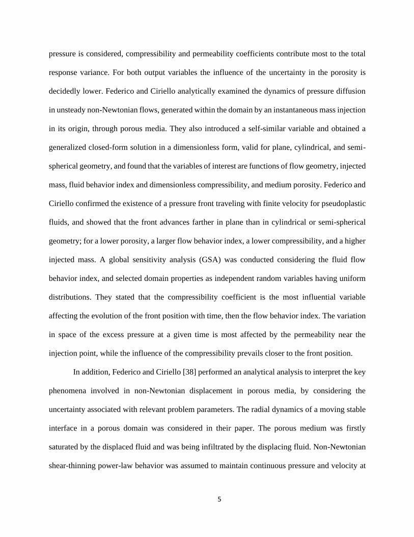
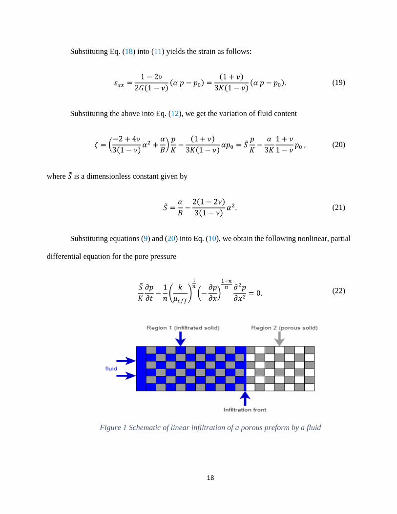
Figure 1 Schematic of linear infiltration of a porous preform by a fluid .................................. 18

Figure 2 Dimensionless Infiltration front versus the applied pressure for 𝑛 = 0.5 .................. 23

Figure 3 Dimensionless Infiltration front versus the applied pressure for 𝑛 = 0.8 .................. 23

Figure 4 Dimensional infiltration front versus time for 𝑛 = 0.5 .............................................. 24

Figure 5 Dimensional infiltration front versus time for 𝑛 = 0.8 .............................................. 24

Figure 6 Normalized pore pressure along the infiltration direction for 𝑛 = 0.5 ...................... 26

Figure 7 Normalized pore pressure along the infiltration direction for 𝑛 = 0.8 ...................... 26

Figure 8 Normalized fluid content variation along the infiltration direction for 𝑛 = 0.5 ........ 27

Figure 9 Normalized fluid content variation along the infiltration direction for 𝑛 = 0.8 ........ 27

Figure 10 Dimensionless Infiltration front versus the inlet flux factor for 𝑛 = 0.5 .................. 31


Figure 12 Dimensional infiltration front versus time for 𝑛 = 0.5 ............................................. 32


Figure 14 Schematic of radial infiltration of a porous preform by a fluid ................................. 34

Figure 15 Dimensionless infiltration front versus applied pressure for 𝑛 = 0.5 ....................... 38

Figure 16 Dimensionless infiltration front versus applied pressure for 𝑛 = 0.8 ....................... 39



Figure 19 Normalized pore pressure along the infiltration direction for 𝑛 = 0.5 ..................... 41

Figure 20 Normalized pore pressure along the infiltration direction for 𝑛 = 0.8 ..................... 41



vii



Figure 25 Schematic of non-isothermal linear infiltration of a porous preform by a fluid ....... 50

Figure 26 Dimensionless Infiltration front versus the applied pressure .................................... 59

Figure 27 Dimensional infiltration front along the time ............................................................ 59

Figure 28 Temperature variation along the infiltration direction .............................................. 60

Figure 29 Normalized pore pressure along the infiltration direction ......................................... 61

Figure 30 Normalized fluid content variation along the infiltration direction ........................... 62

viii

LIST OF SYMBOLS

Symbol Description

𝛼 Biot–Willis coefficient

𝛼𝑓 Volumetric thermal expansion coefficient of the fluid

𝛼𝑠 Volumetric thermal expansion coefficient of the preform

𝐴 Cross section area

𝐵 Skempton’s coefficient

𝑐𝑝 Porous medium compressibility coefficient

𝑐𝑓 Fluid compressibility coefficient

𝑐 Specific heat

𝑐0 Total compressibility coefficient in the flow region

𝛿𝑖𝑗 Kronecker delta

∇2 Laplacian operator

휀 Strain

휂 Dimensionless distance

휂𝑓 Dimensionless infiltration front

휂𝑤 Hole dimensionless distance

𝜐 Drained Poisson’s ratio

𝑓 Body force per unit volume of fluid

𝐹 Body force per unit volume of the bulk material

𝐺 Shear modulus of the drained elastic solid

𝑔 Gravity component

ix

𝐻 Consistency index

ℎ Heat flux

ℎ Hole thickness

𝑟𝑤 Hole radius

𝐾 Drained Bulk modulus

𝜅 Permeability coefficient or mobility coefficient

𝑘𝛼 Thermal conductivity of the fluid phase

𝑘 Intrinsic permeability

𝜆 Thermal conductivity

𝑄𝑤 Inlet flow rate

𝑀𝛼 Connectivity matrix of the fluid phase

𝑀𝛽 Connectivity matrix of the solid phase

𝑛 Flow behavior index

𝜇𝑒𝑓𝑓 Effective viscosity of the fluid

𝜎 Stress

𝑝0 Applied inlet pressure

𝑝 Dimensionless pore pressure

𝑝 Pore pressure

𝜙0 Porosity

𝑞𝑓𝑠 Convection induced heat transfer

𝑞 Fluid flux

x

𝑄0 Injection intensity

𝑄𝑜 Injection intensity

𝑟𝑓 Infiltration front radius

휃 Temperature variation

휃̃ Dimensionless temperature variation

휃0 Inlet temperature

𝑡 Time

𝑢 Displacement

𝑥𝑓 Infiltration front distance

휁 Variation of fluid content

1

1 INTRODUCTION

Newtonian and non-Newtonian fluid flows through porous media are of considerable

interest in several diverse areas; these areas include petroleum, chemical and environmental

engineering, and composite materials manufacturing.

In petroleum engineering, the oil displacement efficiency is improved by using non-

Newtonian displacing fluids [1,2]. Therefore, non-Newtonian fluids, such as shear-thinning

polymer solutions [3,4,5], microemulsions, macroemulsions, and foam solutions [6], are injected

into underground reservoir to improve the efficiency of oil displacement. Another example for

applications in petroleum engineering is the production of heavy crude oils, where the rheological

studies indicated that some of them are also non-Newtonian fluids of power law with yield stress

[7,8,9].

For chemical, environmental, and biomedical engineering applications, non-Newtonian

fluid flow in porous media is applied to the filtration of polymer solutions, soil remediation [10],

food processing [11], and fermentation, through the removal of liquid pollutants. These fluids

occur in many natural and synthetic forms and can be regarded as the rule not the exception [12].

Also, during water flooding operations, chemical additives, polymeric solutions, or foams are

routinely added to the injected water for improving the overall sweeping efficiency and minimizing

the instability effects. Surfactants are also added to the water phase to decrease the surface tension

between the aqueous and oil phases [13]. Another application is the fluid flow in fixed and

fluidised beds of particles, which is encountered in many chemical and processing applications

[16]. In addition, the aqueous solutions of Separan AP‐30, polymethylcellulose, and

polyvinylpyrrolidone were found to exhibit non‐Newtonian flow behavior in simple shear [15]. In

environmental engineering, liquid pollutants and wastes may migrate in the subsurface and

2

penetrate underground reservoirs, leading to groundwater contamination; several of those, such as

suspensions, solutions and emulsions of various substances, certain asphalts and bitumen, greases,

sludges, and slurries, are distinctly non-Newtonian [13]. In Orthopaedic applications, Injectable

bone cements (IBCs) are used in many applications, like poly methyl methacrylate (PMMA),

where bone cements are used for anchoring total joint replacements (TJRs) [14].

In composite materials production, the infiltration process, which is the method of

replacing a fluid (usually vacuum of gas) by another fluid within the pore space of a porous solid

material [20], is being used to manufacture metal matrix composites (MMCs) [5,17], polymer

matrix composites (PMCs) [18,19] and ceramic matrix composites (CMCs) [20,21]. In general,

composites fabrication by infiltration method is one of the most cost-effective and efficient ways

available for many reinforced composite (MMCs, PMCs, or CMCs) [20,22]. An example for the

properties of the CMCs manufactured by infiltration was shown in [23], where SEM observations

of the indentation induced cracks indicated that the polymer network causes much greater crack

deflection than the dense ceramic material.

Flows of Newtonian and non-Newtonian fluids through porous media can be studied by

analytical, numerical, and experimental methods. Many authors have carried out the analytical

studies in flow applications.

In Petroleum Engineering related studies, Pascal [24,25] showed the basic equations

describing the flow through a porous medium of non-Newtonian fluids with a power-law in the

presence of a yield stress. Pascal, also, presented a theoretical analysis for evaluating the effects

of non-Newtonian behavior of the displacing fluid on the interface stability in a radial displacement

in a porous medium and presented some results that demonstrates the theoretical support for the

finding of a strategy regarding the optimal selection of rheological parameters of the displacing

3

fluid. While in [26], Pascal developed approximate analytical solutions for the description of

conditions required for the stability of non-Newtonian fluid interfaces in a porous medium. Pascal

also studied the rheological effects of non-Newtonian fluids in a flow system of a two-phase flow

zone, which are coupled to a single-phase flow zone by a moving fluid interface. The mentioned

flow system is involved in a technique for oil displacement in a porous medium. In addition, Pascal

showed the effects of non-Newtonian displacing fluids, of power law with yield stress, rheological

on the dynamics of a moving interface, which occurs in separating oil from water. Several relevant

conclusions, obtained there, illustrated the conditions in which the viscous fingering effect in oil

displacement could be eliminated and a piston-like displacement may be possible [27,28]. In

addition, Pascal analyzed the non-linear effects associated with unsteady flows through a porous

medium of shear thinning fluids. He showed the existence of a moving pressure front from a self-

similar solution governing the flow behavior. Pascal concluded that the pressure disturbances in a

non-Newtonian fluid flowing through a porous medium propagate with a finite velocity. This

relevant result is in contrast to the infinite velocity of disturbance propagation in a Newtonian fluid

[29]. Finally, in another study, H. Pascal and F. Pascal [30] presented a study related to the

solutions of the nonlinear equations of fluid flow in porous media. These solutions were obtained

by means of a generalized Boltzmann transformation approach for several cases of practical

interest in interpretation of well-flow tests of short duration. They also showed and discussed the

limitations associated with the generalized Boltzmann transformation approach in solving the

nonlinear equations of power law fluid flow in oil reservoirs taking into account the interpretation

of the well-flow test analysis. A formulation of moving boundary problems occurring in the flow-

test analysis of short duration enabled them to obtain the exact analytical solutions in certain cases

of practical interest, like the case of a known constant inlet pressure. However, some limitations

4

associated with the generalized Boltzmann transformation approach arised when the boundary

condition imposed (at the well) was expressed in terms of flow rate instead of a constant pressure.

In that case, the solution in the closed form was obtained only for a certain profile of variable flow

rate in the well.

Chen et al. [33] presented a class of self-similar solutions describing piston-like

displacement of a slightly compressible non-Newtonian, power-law, dilatant fluid by another

through a homogeneous, isotropic porous medium. Their solutions could be used to evaluate the

validity and accuracy of approximate solutions that were existed.

Federico et al. [34] presented a simplified approach to the derivation of an effective

permeability for flow of a purely viscous power–law fluid with flow behavior index n in a

randomly heterogeneous porous domain subjected to a uniform pressure gradient. They concluded

that in 1-D flow, the ratio between effective and mean permeability decreases with increasing

heterogeneity, with a moderate impact of the flow behavior index value, while in 2-D and 3-D

flows, the ratio between effective and mean permeability decreases with increasing log-

permeability variance, except for very pseudoplastic fluids with a flow behavior index smaller than

a limit value depending on flow dimensionality.

Federico and Ciriello [13] also analyzed the dynamics of the pressure variation generated

by an instantaneous mass injection in the origin of a domain, initially saturated by a weakly

compressible non-Newtonian fluid. Coupling the flow law, which is the modified Darcy’s law,

with the mass balance equation yielded the nonlinear partial differential equation governing the

pressure field. After that, an analytical solution was derived as a function of a self-similar variable.

Federico and Ciriello revealed in their analysis that the compressibility coefficient and flow

behavior index are the most influential variables affecting the front position; when the excess

5

pressure is considered, compressibility and permeability coefficients contribute most to the total

response variance. For both output variables the influence of the uncertainty in the porosity is

decidedly lower. Federico and Ciriello analytically examined the dynamics of pressure diffusion

in unsteady non-Newtonian flows, generated within the domain by an instantaneous mass injection

in its origin, through porous media. They also introduced a self-similar variable and obtained a

generalized closed-form solution in a dimensionless form, valid for plane, cylindrical, and semi-

spherical geometry, and found that the variables of interest are functions of flow geometry, injected

mass, fluid behavior index and dimensionless compressibility, and medium porosity. Federico and

Ciriello confirmed the existence of a pressure front traveling with finite velocity for pseudoplastic

fluids, and showed that the front advances farther in plane than in cylindrical or semi-spherical

geometry; for a lower porosity, a larger flow behavior index, a lower compressibility, and a higher

injected mass. A global sensitivity analysis (GSA) was conducted considering the fluid flow

behavior index, and selected domain properties as independent random variables having uniform

distributions. They stated that the compressibility coefficient is the most influential variable

affecting the evolution of the front position with time, then the flow behavior index. The variation

in space of the excess pressure at a given time is most affected by the permeability near the

injection point, while the influence of the compressibility prevails closer to the front position.

In addition, Federico and Ciriello [38] performed an analytical analysis to interpret the key

phenomena involved in non-Newtonian displacement in porous media, by considering the

uncertainty associated with relevant problem parameters. The radial dynamics of a moving stable

interface in a porous domain was considered in their paper. The porous medium was firstly

saturated by the displaced fluid and was being infiltrated by the displacing fluid. Non-Newtonian

shear-thinning power-law behavior was assumed to maintain continuous pressure and velocity at

6

the interface with constant initial pressure. Coupling the nonlinear flow law for both fluids, with

the continuity equation, and taking into account compressibility effects, yielded a set of nonlinear

second-order partial differential equations. Their transformation via a self-similar variable was

done by considering the same flow behavior index for both the displacing and displaced fluids. A

following transformation of the equations including the conditions at the interface has showed for

pseudoplastic fluids the existence of a compression front ahead of the moving interface. Solving

the resulting set of nonlinear equations yielded the moving interface position, the compression

front position, and the pressure distributions which were derived in closed forms for all kinds of

flow behavior. Federico and Ciriello stated that their solution could be used for complex numerical

models, allowed to investigate the key processes and dimensionless parameters involved in non-

Newtonian displacement in porous media, and extended the analytical approach and results of

another different paper of them [8] on flow of a single power-law fluid to motion of two fluids,

taking compressibility effects into account.

WU et al. [6] presented an analytical Buckley-Leverett-type [31] solution for one-

dimensional immiscible displacement of a Newtonian fluid by a non-Newtonian fluid in porous

media. They assumed the viscosity of the non-Newtonian fluid as a function of the flow potential

gradient and the non-Newtonian phase saturation. Where, they developed a practical procedure for

applying their method to field problems which is based on the analytical solution, similar to the

graphic technique of Welge [32]. Their solution could be regarded as an extension of the Buckley-

Leverett method to Non-Newtonian fluids. The results obtained by their analytical analysis

revealed how the saturation profile and the displacement efficiency could be controlled by the

relative permeabilities and by the inherent complexities of the non-Newtonian fluid. A couple

examples of the application for their analytical solution were submitted in that research study. The

7

first one is the effect analysis of non-Newtonian behavior on immiscible displacement of a

Newtonian fluid by a power-law non-Newtonian fluid. The second one is a verification of the

numerical model for simulation of flow of immiscible non-Newtonian and the Newtonian fluids

in porous media. Good agreement between the analytical and the numerical results was shown.

For complicated displacements of fluid in porous media, according to Walsh et al [43], the

easiest way to understand it is through fractional flow theory, which is an application of a subset

of the method of characteristics (MOC). Walsh et al extended the fractional flow theory

understanding to the displacement of oil by a miscible solvent in the presence of an immiscible

aqueous phase. The fractional flow theory was generalized by Pope [44], starting with the Buckley-

Leverett theory for waterflooding, his mathematics have been based on the MOC. Pope also treated

three-phase flow problems, which occurs in a variety of the EOR processes. While Rossen et al.

[44] extended fractional flow methods for two-phase flow to non-Newtonian fluids in a cylindrical

one-dimensional flow. They also analyzed the characteristic equations for the polymer applications

and foam floods applications.

For composites infiltration related studies, the infiltration process is governed by the

phenomena of fluid flow, capillarity, and the mechanics of potential preform deformation. These

phenomena are governed by four basic parameters: viscosity of the liquid melt phase, the pressure

dependent melt saturation in the preform, the preform permeability and porosity, and the preform

stress strain behavior. Comparing these parameters, in particular of surface tension and viscosity

values, across all matrix material classes indicated clear differences, explaining the main

differences in the engineering practice from a composite matrix to another. However, the

governing laws are the same [20].

8

Michaud et al. [20] reviewed the phenomena and the governing laws for the case of

isothermal infiltration of a porous preform by a Newtonian fluid without a phase transformation,

and four basic functional quantities were addressed. They presented some examples of model

methodologies and compared them with the available experimental data. They also illustrated the

applications of these governing laws using the analytical and numerical methods.

In another paper Michaud et al. [56] analyzed the infiltration by a pure matrix considering

preform deformation and partial matrix solidification and studied the superheat influence within

the infiltration metal, neglecting the pressure drop in the remelted region. They concluded that the

superheat had only a minor effect on the infiltration kinetics, which is the same result of a rigid

preform case, but the superheat significantly affected the remelted region length. Another

conclusion of their work was that using a bounding approach, the upper bound, which ignored the

solid metal influence on the preform relaxation, and lower bound, which assumed that the solid

metal conferred complete rigidity to the preform, were close compared to other factors of

uncertainty in the infiltration prediction. Finally, they concluded that neglecting the solid phase

velocity for the liquid velocity and considering the melt superheat to be zero could bound the

infiltration rate to become relatively simple to be calculated with good precision

In a study related to the manufacturing of metal matrix composites (MMCs), Lacoste et al.

[39] pointed out the analogous numerical studies of the Resin Transfer Moulding (RTM) process

and listed some technological difficulties which has encountered this process, in particular due to

the appearance of many complex phenomena during processing. That analysis has included

deformation of the fibrous preform, phase change of metal, and microporosities. They also

presented some examples regarding the limits and possibilities offered by the numerical modelling.

9

In addition, they pointed out to some conditions that must be satisfied. As for the quality of the

numerical simulation, they said it depends on the relevance of the used physical parameters.

Jung et al. [40] developed an axisymmetric finite element (FE) model for the process of

squeeze casting the MMCs. They have numerically studied the flow in the mold, the infiltration

into the porous preform, and the solidification of the molten metal. They used a simple preform

deformation model to predict the permeability change caused by preform compression during

infiltration. In addition, they did a series of infiltration experiments to validate the assumptions

used in the numerical model. The comparison between the experimental and numerical data

showed that the developed FE program successfully predicts the actual squeeze casting process.

Jung et al. concluded that the higher the preheat temperature of the metal and the mold, the lower

the infiltration pressure required, and the lower metal pressure results in less preform deformation.

For the properties of CMCs, which are usually manufactured by infiltration, Prielipp et al.

[41] described the mechanical properties of metal reinforced ceramics, especially AI/A1203

composites with interpenetrating networks. Fracture strength and fracture toughness data were

given as functions of two variables; ligament diameter and fiber volume fraction. Then, they

compared their results with the corresponding values of the porous preforms. They also presented

a simple model for accounting the influence of metal volume and metal ligament diameter on the

composites’ toughness. Their results showed that the increase in fracture strength from the porous

preform to the composite is much larger than the increase of the fracture toughness increase alone,

and the fracture strength of that material is increased more by metal infiltration than the plateau

toughness derived from long crack measurements.

Jin [42] described a thermo-poroelasticity theory to investigate the effects of temperature

gradients on the infiltration kinetics, pore pressure distribution of the liquid phase, and liquid

10

content variation due to preform deformation for infiltration processing of interpenetrating phase

composites. He also derived a similarity solution for one-dimensional infiltration assuming no

solidification of the liquid phase and showed that the infiltration front also depends on the

poroelastic properties of the preform. A numerical example for a polymer–ceramic

interpenetrating phase composite was presented and the results showed that the temperature

gradients may produce significant liquid content increment beyond the amount that can be

accommodated by the initial pore volume of the preform. This increment in liquid content may

compensate some solidification shrinkage of the liquid phase and alter thermal residual stresses,

thereby reducing occurrence of microdefects in the composite.

As reviewed above, flows of non-Newtonian fluids in porous media have been studied

extensively. However, only Newtonian fluid has been used in the study of infiltration processing

of composite materials (Jin [42], Michaud et al. [20], Jung et al. [40], Ouahbi et al. [22], Ambrosi

[46] and Larsson et al. [47]. In the infiltration processing of composites, the fluid phase is a molten

polymer or metal. Many polymers, however, are non-Newtonian fluids in the molten state

[48,49,50]. Therefore, non-Newtonian fluid models should be used to better understand the melt

flow behavior and solid preform deformation in the study of infiltration processing of composite

materials. In addition, the infiltration front has been a major concern in the infiltration processing

of composite materials. The objective of this thesis is to study infiltration processing of

interpenetrating composites using a non-Newtonian fluid model. Both one-dimensional linear and

radial flow of a non-Newtonian fluid in a porous preform will be studied. Equations to determine

the non-dimensional isothermal infiltration front as a function of the known inlet boundary

condition, i.e., inlet pressure or inlet fluid flux factor, are derived, and numerical examples are

presented. Besides isothermal infiltration of a porous preform by a non-Newtonian fluid, non-

11

isothermal infiltration by a Newtonian fluid with convection heat transfer (which was ignored in

[42]) is also studied numerically.

The organization of this thesis is as follows:

The first chapter introduces non-Newtonian fluid flow in porous media and reviews the

previous work in this area with applications in petroleum engineering, chemical engineering and

composite manufacturing.

In chapter 2, the isothermal linear infiltration of a porous solid by a non-Newtonian fluid

is presented and the basic equations of 3-dimensional poroelasticiy are presented in the first section

of this chapter. Then, the equations are reduced to one-dimensional flow in the second section. A

self-similarity solution for a specified inlet pressure boundary condition and a numerical example,

for a ceramic porous preform and a melted polymer, are presented in the third section of this

chapter. While a self-similarity solution for a specified inlet flow rate boundary condition and a

numerical example, with material parameters consistent with those of the third section, are

presented in the fourth section of the chapter.

In chapter 3, the isothermal radial infiltration of a porous solid by a non-Newtonian fluid

is presented and the basic equations of 3-dimensional poroelasticiy are presented in the first section

of this chapter. Then, the equations are reduced to one-dimensional flow in the second section. A

self-similarity solution for a specified inlet pressure boundary condition and a numerical example,

for data consistent with the data of linear flow application, are presented in the third section of this

chapter. While in the fourth section, a self-similarity solution for a specified inlet flow rate

boundary condition and a numerical example, for data consistent with the data of linear flow

application, are presented.

12

In chapter 4, the non-isothermal linear infiltration of a porous solid by a Newtonian fluid

is presented, basic equations of 3-dimensional thermo-poroelasticiy are presented in the first

section. Then, they are reduced to one-dimensional flow in the second section. A self-similarity

solution for a specified inlet pressure boundary condition and a numerical example with convection

heat transfer are presented in the third section of that chapter.

The fifth chapter incorporates the conclusions which could be obtained from the presented

work.

13

2 ISOTHERMAL LINEAR FLOW OF A NON-NEWTONIAN FLUID IN A POROUS

MEDIUM

2.1 Basic Equations of Poroelasticity

Fluid transport in the interstitial space in a porous solid can be described by the well-known

Darcy’s law which is an empirical equation for seepage flow in non-deformable porous media. It

can also be derived from Navier-Stokes equations by dropping the inertial terms. Consistent with

the current small deformation assumptions and by ignoring the fluid density variation effect

(Hubert’s Potential) [51]. Modified Darcy’s law for non-Newtonian flow can be adopted here

𝑞𝑖 = −𝜅(𝑝,𝑖− 𝑓𝑖)1𝑛, (1)

In the above equation, 𝑞𝑖 is the specific discharge vector, or fluid flux vector, which describes the

motion of the fluid relative to the solid and is formally defined as the rate of fluid volume crossing

a unit area of porous solid whose normal is in the 𝑥𝑖 direction, 𝑓𝑖 = 𝜌𝑓𝑔𝑖 the body force per unit

volume of fluid (with 𝜌𝑓 the fluid density, and 𝑔𝑖 the gravity component in the 𝑖-direction), 𝑝 the

pore pressure, and 𝜅 = 𝑘 𝜇𝑒𝑓𝑓⁄ the permeability coefficient or mobility coefficient (with 𝑘 the

intrinsic permeability having dimension of length squared, and 𝜇𝑒𝑓𝑓 the effective viscosity of the

fluid).

The following conventions have been adopted in writing the basic equations: a comma

followed by subscripts denotes differentiation with respect to spatial coordinates and repeated

indices in the same monomial imply summation over the range of the indices (generally 𝑥, 𝑦 and

𝑧, unless otherwise indicated).

14

The effective viscosity of the fluid is given by Ref. [30]

𝑘

𝜇𝑒𝑓𝑓=

1

2𝐻(

𝑛𝜙0

3𝑛 + 1)

𝑛

(8𝑘

𝜙0)

(1+𝑛) 2⁄

, (2)

where 𝐻 is the consistency index, 𝑛 the flow behavior index with 𝑛 < 1, = 1, or > 1 describing

respectively pseudoplastic, Newtonian, or dilatant behavior, and 𝜙0 the porosity. The porosity is

assumed to be a constant like in the classical small deformation poroelasticity [42].

Two “strain” quantities are also introduced to describe the deformation and the change of

fluid content of the porous solid with respect to an initial state: the usual small strain tensor 휀𝑖𝑗 and

the variation of fluid content 휁, defined as the variation of fluid volume per unit volume of porous

material: 휀𝑖𝑗 is positive for extension, while a positive 휁 corresponds to a “gain” of fluid by the

porous solid [51]. The strain tensor is related to the original kinematic variables 𝑢𝑖, the solid

displacement vector that tracks the movement of the porous solid with respect to a reference

configuration according to the following strain-displacement relations

휀𝑖𝑗 =1

2(𝑢𝑖,𝑗 + 𝑢𝑗,𝑖). (3)

The fluid flux vector and the variation of fluid content satisfy the following continuity

equation

𝜕휁

𝜕𝑡= −𝑞𝑖,𝑖 , (4)

where 𝑡 is the time.

For flow of an incompressible fluid, the fluid content variation is solely due to the

deformation of the porous preform [42].

15

The stress and strain follow the constitutive equations in the framework of Biot theory [42]

𝜎𝑖𝑗 + 𝛼𝑝𝛿𝑖𝑗 = 2𝐺휀𝑖𝑗 +2𝐺𝜐

1 − 2𝜐휀𝑘𝑘𝛿𝑖𝑗 , (5)

2𝐺휁 =𝛼(1 − 2𝜐)

1 + 𝜐(𝜎𝑘𝑘 +

3

𝐵𝑝), (6)

where 𝜎𝑖𝑗 is the total stress tensor, 𝛼 identified as the Biot–Willis coefficient, 𝐺 the shear modulus

of the drained elastic solid, 𝜐 the drained Poisson’s ratio, 𝐵 the Skempton’s coefficient, and 𝛿𝑖𝑗 the

Kronecker delta.

Finally, the following equilibrium equations supplement the basic governing equations of

poroelasticity [42]

𝜎𝑖𝑗,𝑗 = −𝐹𝑖 , (7)

where 𝐹𝑖 = 𝜌𝑔𝑖 is the body force per unit volume of the bulk material.

2.2 Basic Equations for One-Dimensional Flow

In this section, we consider one-dimensional (1-D) isothermal infiltration of a porous solid

by a non-Newtonian fluid in the 𝑥-direction as schematically shown in Figure 1. At a given

moment of infiltration, the porous preform is divided into two regions, i.e., Region 1 in which the

preform is infiltrated by the fluid, and Region 2 in which the preform has not yet been infiltrated.

The two regions are separated by the moving infiltration front. In applications, infiltration can

occur with three kinds of known boundary conditions. In the first case, which is termed the 𝑝0 −

𝑝𝑓 problem, infiltration is driven by a specified fluid pressure at the inlet, 𝑥 = 0, and the pressure

16

at the infiltration front is also given. In the second case, which is termed the 𝑄0 − 𝑝𝑓 problem, the

fluid flow in the porous preform is caused by a specified flow rate at the inlet, 𝑥 = 0, with the pore

pressure specified at the other end. Finally, the third case in which the flow rates are specified at

both ends and is termed the 𝑄0 − 𝑄𝑓 problem [30]. The first 2 cases will be discussed in this thesis.

In the 1-D problems, we assume that no lateral deformation and fluid flow occur, which

corresponds to infiltration of the preform confined by a rigid and impermeable mold. Moreover,

the body force is not considered. Hence, the following strain and fluid flux components are zero

휀𝑦𝑦 = 휀𝑧𝑧 = 휀𝑥𝑦 = 휀𝑦𝑧 = 휀𝑥𝑦 = 𝑢𝑦 = 𝑢𝑧 = 0,

𝑞𝑦 = 𝑞𝑧 = 0.

(8a)

(8b)

Moreover, all field variables are functions of 𝑥 and time 𝑡, for example, the pore pressure

field is 𝑝 = 𝑝(𝑥, 𝑡). Under the above 1-D isothermal infiltration assumptions, the constitutive

equations in (01), (4), (5), (6) and (7) reduce to

𝑞𝑥 = (−𝑘

𝜇𝑒𝑓𝑓

𝜕𝑝

𝜕𝑥)

1𝑛

, (9)

𝜕휁

𝜕𝑡+

𝜕𝑞𝑥

𝜕𝑥= 0, (10)

𝜎𝑥𝑥 = 2𝐺1 − 𝜈

1 − 2𝜈휀𝑥𝑥 − 𝛼 𝑝, (11)

휁 = 𝛼휀𝑥𝑥 + (−𝛼2

𝐾 +

𝛼

𝐾𝐵) 𝑝, (12)

𝜕𝜎𝑥𝑥

𝜕𝑥= 0, (13)

where 𝐾 is the drained Bulk modulus.

17

Designated boundary conditions at the inlet, 𝑥 = 0, are either constant pressure 𝑝0 or flow

rate 𝑄𝑤(𝑡)

or

𝑝 = 𝑝0, 𝑥 = 0,

𝑞𝑥 =𝑄𝑤(𝑡)

𝐴, 𝑥 = 0,

(14a)

(14b)

where 𝐴 is the cross section area of the porous preform, and

𝑄𝑤(𝑡) = 𝑄0𝑡𝑐 , (15)

where 𝑄0 is the injection intensity and 𝑐 a real number.

The boundary condition at the infiltration front is

𝑝 = 𝑝𝑓 = 0, 𝑥 = 𝑥𝑓 , (16)

where 𝑥𝑓 is the infiltration front, and will be determined later.

Lastly, the stress 𝜎𝑥𝑥 at the inlet is known to be

𝜎𝑥𝑥 = −𝑝0, 𝑥 = 0. (17)

The above boundary conditions need to be supplemented by the continuity of stress 𝜎𝑥𝑥

and displacement 𝑢𝑥 at the infiltration front. It follows from the equilibrium equation (13) that the

stress 𝜎𝑥𝑥 is a constant which is determined by the boundary condition (17) as −𝑝0. We thus have

the following normal stress along the infiltration direction

𝜎𝑥𝑥 = −𝑝0, 0 ≤ 𝑥 ≤ 𝑥𝑓 . (18)

18

Substituting Eq. (18) into (11) yields the strain as follows:

휀𝑥𝑥 =1 − 2𝜈

2𝐺(1 − 𝜈)(𝛼 𝑝 − 𝑝0) =

(1 + 𝜈)

3𝐾(1 − 𝜈)(𝛼 𝑝 − 𝑝0). (19)

Substituting the above into Eq. (12), we get the variation of fluid content

휁 = (−2 + 4𝜈

3(1 − 𝜈)𝛼2 +

𝛼

𝐵)

𝑝

𝐾−

(1 + 𝜈)

3𝐾(1 − 𝜈)𝛼𝑝0 = �̃�

𝑝

𝐾−

𝛼

3𝐾

1 + 𝜈

1 − 𝜈𝑝0 , (20)

where �̃� is a dimensionless constant given by

�̃� =𝛼

𝐵−

2(1 − 2𝜈)

3(1 − 𝜈)𝛼2. (21)

Substituting equations (9) and (20) into Eq. (10), we obtain the following nonlinear, partial

differential equation for the pore pressure

�̃�

𝐾

𝜕𝑝

𝜕𝑡−

1

𝑛(

𝑘

𝜇𝑒𝑓𝑓)

1𝑛

(−𝜕𝑝

𝜕𝑥)

1−𝑛𝑛 𝜕2𝑝

𝜕𝑥2= 0. (22)

Figure 1 Schematic of linear infiltration of a porous preform by a fluid

19

2.3 The 𝒑𝟎 − 𝒑𝒇 Problem

2.3.1 A Self-Similarity Solution

Following [42], we seek a similarity solution for the problem. Introduce a dimensionless

distance 휂 as follows:

휂 = 𝑥 (𝑘

𝜇𝑒𝑓𝑓𝐾)

−1𝑛+1

𝑡−𝑛

𝑛+1, (23)

In the similarity solution, the pore pressure has the following form

𝑝(𝑥, 𝑡) = 𝑝0𝑝(휂), (24)

where 𝑝 is a dimensionless pore pressure and is a function of 휂 only.

The basic equation (22) and the boundary conditions for the pore pressure now become

𝑑2𝑝

𝑑휂2−

𝑛2

𝑛 + 1(

𝑝0

𝐾)

𝑛−1𝑛

�̃�휂 (−𝑑𝑝

𝑑휂)

2𝑛−1𝑛

= 0, (25)

𝑝 = 1, 휂 = 0, (26)

𝑝 = 0, 휂 = 휂𝑓 , (27)

where 휂𝑓 is a constant and related to the infiltration front 𝑥𝑓 by

휂𝑓 = 𝑥𝑓 (𝑘


−1𝑛+1

𝑡−𝑛

𝑛+1. (28)

20

Integrating Eq. (25) yields

𝑑𝑝

𝑑휂= − [𝐶1 −

𝑛(1 − 𝑛)

2(𝑛 + 1)(

𝑝0

𝐾)

𝑛−1𝑛

�̃�휂2]

𝑛1−𝑛

, (29)

where 𝐶1 is an integration constant.

The solution of Eq. (29) under the boundary conditions (26) is

𝑝(휂) = 1 − ∫ [𝐶1 −𝑛(1 − 𝑛)

2(𝑛 + 1)(

𝑝0

𝐾)

𝑛−1𝑛

�̃�휂2]

𝑛1−𝑛𝜂

0

𝑑휂. (30)

Using the boundary condition (27) in (30), we obtain the following equation satisfied by

the integration constant 𝐶1

1 − ∫ [𝐶1 −𝑛(1 − 𝑛)

2(𝑛 + 1)(

𝑝0

𝐾)

𝑛−1𝑛

�̃�휂2]

𝑛1−𝑛𝜂𝑓

0

𝑑휂 = 0. (31)

The constant 𝐶1 can be expressed in terms of 휂𝑓 and 𝑝0 by the condition

𝑑𝑥𝑓

𝑑𝑡=

1

𝜙0𝑞𝑥|𝑥=𝑥𝑓

, (32)

i.e., the velocity of the infiltration front is the fluid flux at the front divided by the porosity𝜙0[42].

𝐶1 = 휂𝑓1−𝑛 (

𝑛 + 1

𝑛𝜙0)

𝑛−1

(𝑝0

𝐾)

𝑛−1𝑛

+𝑛(1 − 𝑛)

2(𝑛 + 1)(

𝑝0

𝐾)

𝑛−1𝑛

�̃�휂𝑓2 . (33)

21

Substituting 𝐶1 in Eq. (33) into Eq. (31), we obtain

∫ [휂𝑓1−𝑛 (

𝑛 + 1

𝑛𝜙0)

𝑛−1

+𝑛(1 − 𝑛)

2(𝑛 + 1)�̃�(휂𝑓

2 − 휂2)]

𝑛1−𝑛𝜂𝑓

0

𝑑휂 −𝑝0

𝐾= 0. (34)

The above is the equation to determine the non-dimensional infiltration front 휂𝑓 as a

function of the applied initial pressure 𝑝0.

2.3.2 Numerical Results and Discussion

This section presents numerical examples of the non-dimensional infiltration front 휂𝑓

versus the applied inlet pressure 𝑝0, the dimensional infiltration front 𝑥𝑓 as a function of time 𝑡,

the normalized pore pressure 𝑝 along the infiltration direction 휂, and the normalized liquid

content variation 휁 (𝑝0 𝐾⁄ )⁄ along the infiltration direction 휂. Table 1 lists the poroelastic

parameters for the fluid-filled porous medium in the numerical calculations [42]. The liquid

phase is a molten polymer and the preform is a ceramic material for possible dental applications.

The viscosity value is chosen to be 0.1 𝑃𝑎. 𝑠, which is the viscosity for Epoxy during infiltration

[20]. Molten polymers have a viscosity range from 0.1 𝑃𝑎. 𝑠 (for typical uncured thermoset

matrices) to 104 𝑃𝑎. 𝑠 (for thermoplastic polymers) [20]. The results are shown for 2 values of

flow behavior index, 𝑛 = 0.5 and 𝑛 = 0.8. The flow behavior index of commercial polymers

varies between 0.2 and 0.8 [57].

The infiltration front is the most important quantity in the infiltration processing of

composite materials [42]. Figure 2 shows, for 𝑛 = 0.5, the non-dimensional infiltration front 휂𝑓

versus the applied fluid pressure 𝑝0, with various values of the preform porosity. While Figure 3

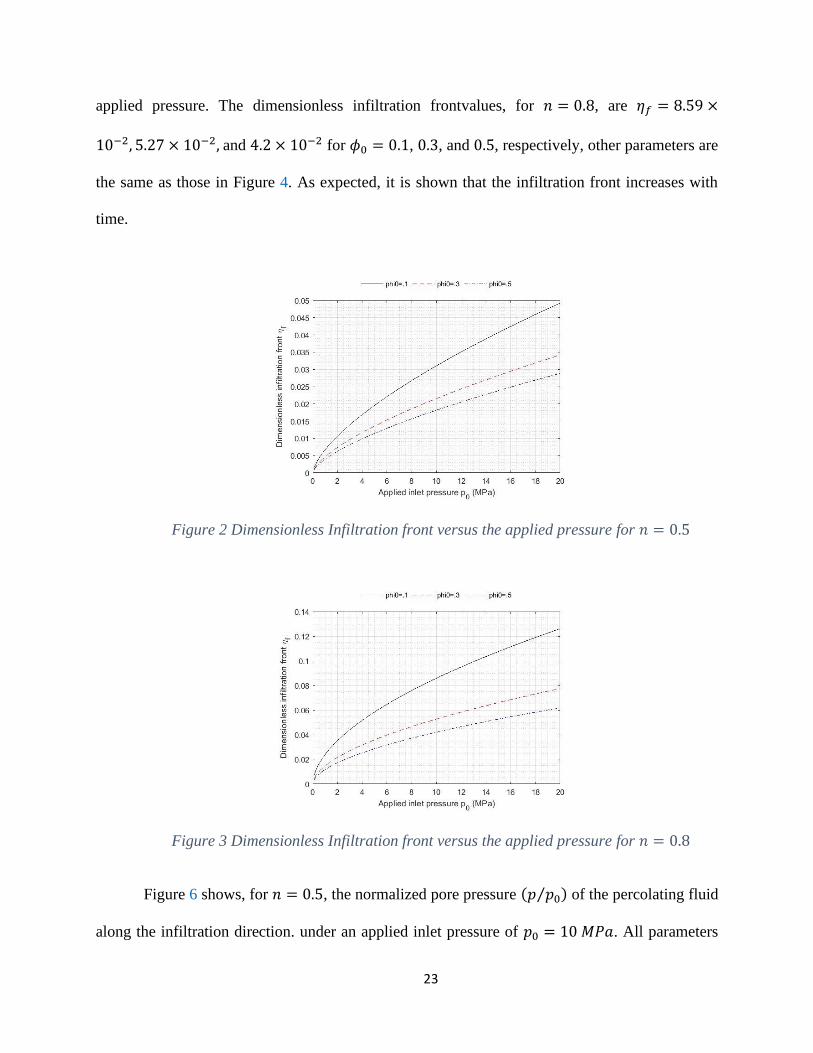
shows the results for 𝑛 = 0.8. It is shown, as expected, that the non-dimensional infiltration front

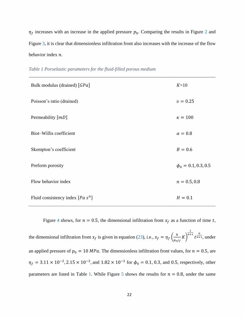
22

휂𝑓 increases with an increase in the applied pressure 𝑝0. Comparing the results in Figure 2 and

Figure 3, it is clear that dimensionless infiltration front also increases with the increase of the flow

behavior index 𝑛.

Table 1 Poroelastic parameters for the fluid-filled porous medium

Bulk modulus (drained) [𝐺𝑃𝑎] 𝐾=10

Poisson’s ratio (drained) 𝜐 = 0.25

Permeability [𝑚𝐷] 𝜅 = 100

Biot–Willis coefficient 𝛼 = 0.8

Skempton’s coefficient 𝐵 = 0.6

Preform porosity 𝜙0 = 0.1, 0.3, 0.5

Flow behavior index 𝑛 = 0.5, 0.8

Fluid consistency index [𝑃𝑎 𝑠𝑛] 𝐻 = 0.1

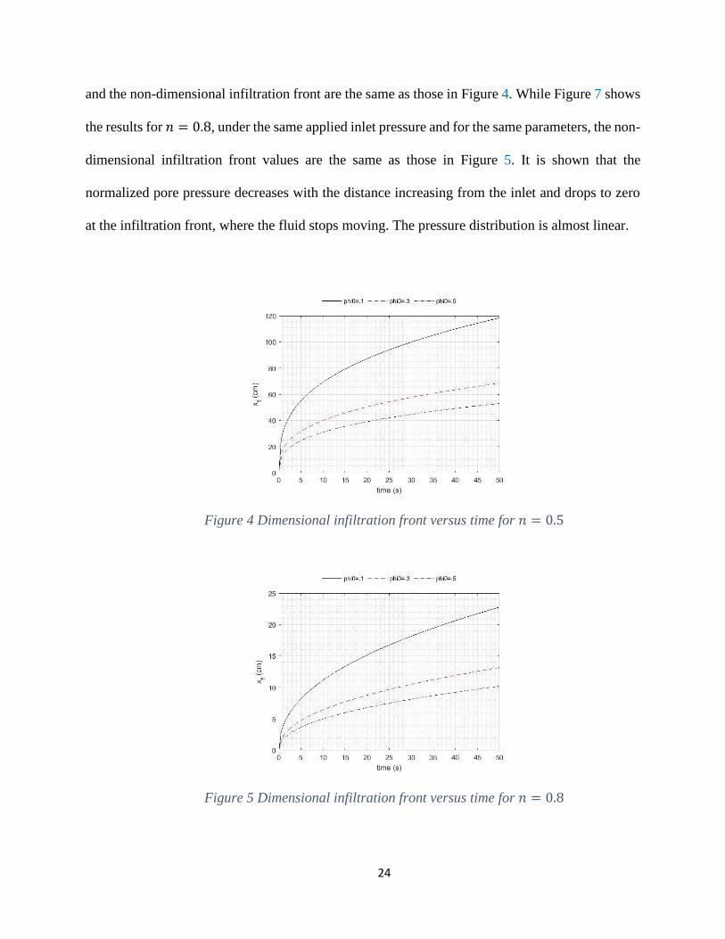
Figure 4 shows, for 𝑛 = 0.5, the dimensional infiltration front 𝑥𝑓 as a function of time 𝑡,

the dimensional infiltration front 𝑥𝑓 is given in equation (23), i.e., 𝑥𝑓 = 휂𝑓 (𝑘


1

𝑛+1𝑡

𝑛

𝑛+1, under

an applied pressure of 𝑝0 = 10 𝑀𝑃𝑎. The dimensionless infiltration front values, for 𝑛 = 0.5, are

휂𝑓 = 3.11 × 10−2, 2.15 × 10−2, and 1.82 × 10−2 for 𝜙0 = 0.1, 0.3, and 0.5, respectively, other

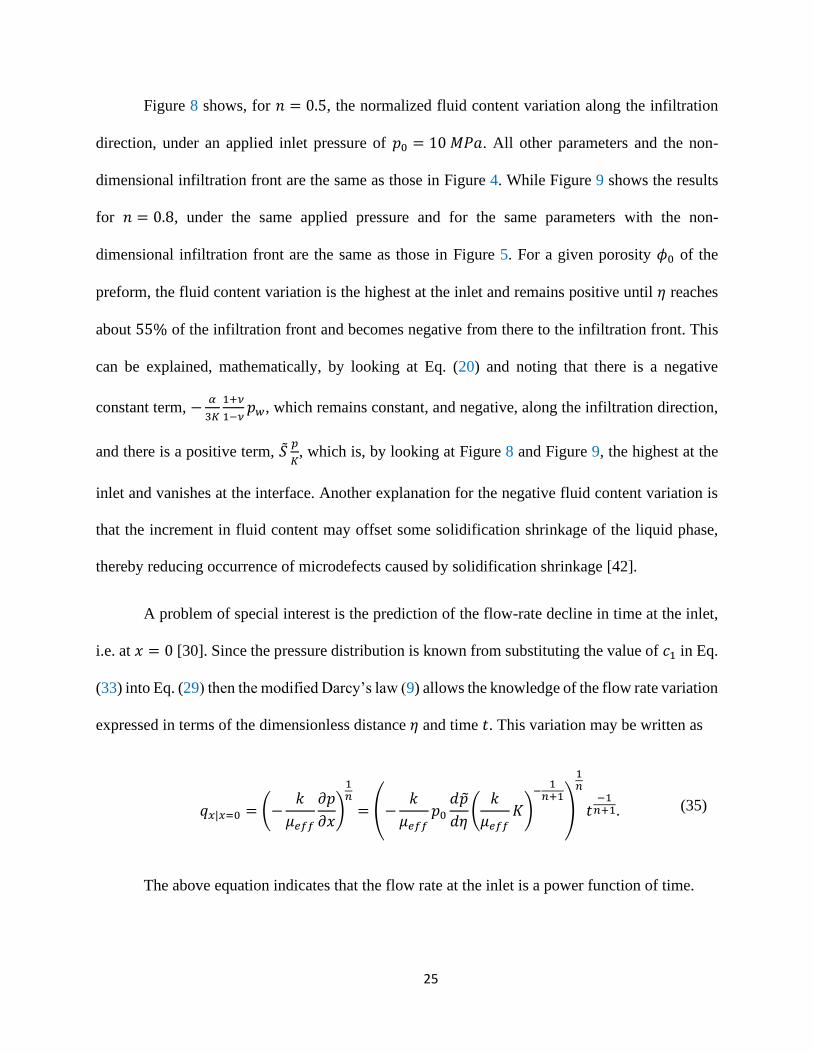
parameters are listed in Table 1. While Figure 5 shows the results for 𝑛 = 0.8, under the same

23

applied pressure. The dimensionless infiltration frontvalues, for 𝑛 = 0.8, are 휂𝑓 = 8.59 ×

10−2, 5.27 × 10−2, and 4.2 × 10−2 for 𝜙0 = 0.1, 0.3, and 0.5, respectively, other parameters are

the same as those in Figure 4. As expected, it is shown that the infiltration front increases with

time.

Figure 2 Dimensionless Infiltration front versus the applied pressure for 𝑛 = 0.5

Figure 3 Dimensionless Infiltration front versus the applied pressure for 𝑛 = 0.8

Figure 6 shows, for 𝑛 = 0.5, the normalized pore pressure (𝑝 𝑝0⁄ ) of the percolating fluid

along the infiltration direction. under an applied inlet pressure of 𝑝0 = 10 𝑀𝑃𝑎. All parameters

24

and the non-dimensional infiltration front are the same as those in Figure 4. While Figure 7 shows

the results for 𝑛 = 0.8, under the same applied inlet pressure and for the same parameters, the non-

dimensional infiltration front values are the same as those in Figure 5. It is shown that the

normalized pore pressure decreases with the distance increasing from the inlet and drops to zero

at the infiltration front, where the fluid stops moving. The pressure distribution is almost linear.

Figure 4 Dimensional infiltration front versus time for 𝑛 = 0.5


25

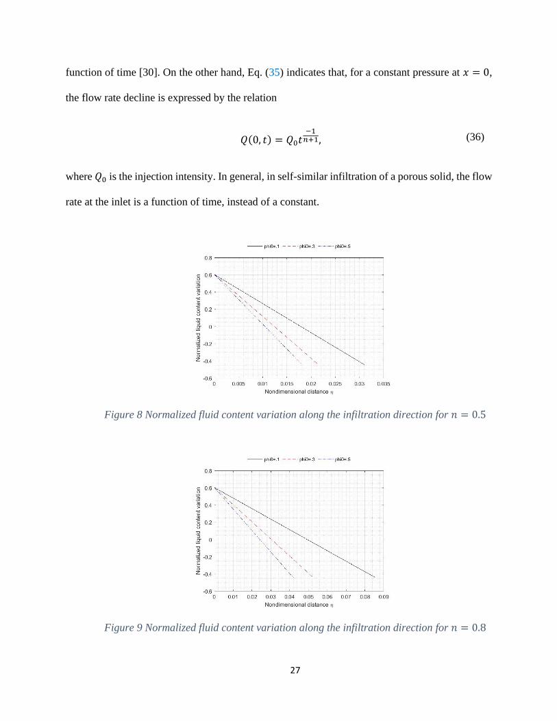
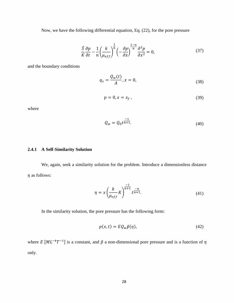
Figure 8 shows, for 𝑛 = 0.5, the normalized fluid content variation along the infiltration

direction, under an applied inlet pressure of 𝑝0 = 10 𝑀𝑃𝑎. All other parameters and the non-

dimensional infiltration front are the same as those in Figure 4. While Figure 9 shows the results

for 𝑛 = 0.8, under the same applied pressure and for the same parameters with the non-

dimensional infiltration front are the same as those in Figure 5. For a given porosity 𝜙0 of the

preform, the fluid content variation is the highest at the inlet and remains positive until 휂 reaches

about 55% of the infiltration front and becomes negative from there to the infiltration front. This

can be explained, mathematically, by looking at Eq. (20) and noting that there is a negative

constant term, −𝛼

3𝐾

1+𝜈

1−𝜈𝑝𝑤, which remains constant, and negative, along the infiltration direction,

and there is a positive term, �̃�𝑝

𝐾, which is, by looking at Figure 8 and Figure 9, the highest at the

inlet and vanishes at the interface. Another explanation for the negative fluid content variation is

that the increment in fluid content may offset some solidification shrinkage of the liquid phase,

thereby reducing occurrence of microdefects caused by solidification shrinkage [42].

A problem of special interest is the prediction of the flow-rate decline in time at the inlet,

i.e. at 𝑥 = 0 [30]. Since the pressure distribution is known from substituting the value of 𝑐1 in Eq.

(33) into Eq. (29) then the modified Darcy’s law (9) allows the knowledge of the flow rate variation

expressed in terms of the dimensionless distance 휂 and time 𝑡. This variation may be written as

𝑞𝑥|𝑥=0 = (−𝑘

𝜇𝑒𝑓𝑓

𝜕𝑝

𝜕𝑥)

1𝑛

= (−𝑘

𝜇𝑒𝑓𝑓𝑝0

𝑑𝑝

𝑑휂(

𝑘


−1

𝑛+1

)

1𝑛

𝑡−1

𝑛+1. (35)

The above equation indicates that the flow rate at the inlet is a power function of time.

26

Figure 6 Normalized pore pressure along the infiltration direction for 𝑛 = 0.5


2.4 The 𝑸𝟎 − 𝒑𝒇 Problem

In practice, instead of a constant pressure of production at the inlet, a variable flow rate

𝑄0𝑡𝑐, may also be given at the inlet to drive the fluid flow in the porous media. In this case,

knowledge of pressure variation in time at the outface flow is of great practical interest. As field

observations have shown, the flow rate at the outface flow declines as a continuous monotonic

27

function of time [30]. On the other hand, Eq. (35) indicates that, for a constant pressure at 𝑥 = 0,

the flow rate decline is expressed by the relation

𝑄(0, 𝑡) = 𝑄0𝑡−1

𝑛+1, (36)

where 𝑄0 is the injection intensity. In general, in self-similar infiltration of a porous solid, the flow

rate at the inlet is a function of time, instead of a constant.

Figure 8 Normalized fluid content variation along the infiltration direction for 𝑛 = 0.5

Figure 9 Normalized fluid content variation along the infiltration direction for 𝑛 = 0.8

28

Now, we have the following differential equation, Eq. (22), for the pore pressure

�̃�

𝐾

𝜕𝑝

𝜕𝑡−

1

𝑛(

𝑘

𝜇𝑒𝑓𝑓)

1𝑛

(−𝜕𝑝

𝜕𝑥)

1−𝑛𝑛 𝜕2𝑝

𝜕𝑥2= 0, (37)

and the boundary conditions


𝐴, 𝑥 = 0, (38)

𝑝 = 0, 𝑥 = 𝑥𝑓 , (39)

where

𝑄𝑤 = 𝑄0𝑡−1

𝑛+1. (40)


We, again, seek a similarity solution for the problem. Introduce a dimensionless distance

휂 as follows:

휂 = 𝑥 (𝑘


−1𝑛+1

𝑡−𝑛

𝑛+1. (41)

In the similarity solution, the pore pressure has the following form:

𝑝(𝑥, 𝑡) = 𝐸𝑄𝑤�̃�(휂), (42)

where 𝐸 [𝑀𝐿−4𝑇−1] is a constant, and 𝑝 a non-dimensional pore pressure and is a function of 휂

only.

29

Using the dimensionless variables, the basic equation (37) and the boundary conditions for

the pore pressure now become

𝑑2𝑝

𝑑휂2− (

𝐸𝑄𝑤

𝐾)

𝑛−1𝑛 𝑛2

𝑛 + 1�̃�휂 (−

𝑑𝑝

𝑑휂)

2𝑛−1𝑛

= 0, (43)


𝐴, 휂 = 0, (44)

𝑝 = 0, 휂 = 휂𝑓 . (45)

Integrating Eq. (43), we get

𝑑𝑝

𝑑휂= − [𝐶2 −

𝑛(1 − 𝑛)

2(𝑛 + 1)(

𝐸𝑄𝑤

𝐾)

𝑛−1𝑛

�̃�휂2]

𝑛1−𝑛

, (46)

where 𝐶2 is an integration constant. Using the following infiltration front condition

𝑑𝑥𝑓

𝑑𝑡=

1

𝜙0𝑞𝑥|𝑥=𝑥𝑓

. (47)

the constant 𝐶2 can be determined as follows:

𝐶2 = 휂𝑓1−𝑛 (

𝑛 + 1

𝑛𝜙0)

𝑛−1

(𝐸𝑄𝑤

𝐾)

𝑛−1𝑛

+𝑛(1 − 𝑛)

2(𝑛 + 1)(

𝐸𝑄𝑤

𝐾)

𝑛−1𝑛

�̃�휂𝑓2 . (48)

Substituting 𝐶2 in Eq. (48) into Eq. (4648), we obtain

30

𝑑𝑝

𝑑휂= − [휂𝑓

1−𝑛 (𝑛 + 1

𝑛𝜙0)

𝑛−1

(𝐸𝑄𝑤

𝐾)

𝑛−1𝑛

+𝑛(1 − 𝑛)

2(𝑛 + 1)(

𝐸𝑄𝑤

𝐾)

𝑛−1𝑛

�̃�휂𝑓2

−𝑛(1 − 𝑛)

2(𝑛 + 1)(

𝐸𝑄𝑤

𝐾)

𝑛−1𝑛

�̃�휂2]

𝑛1−𝑛

.

(49)

Using the boundary condition (44) and Eqs. (36), (49) and (9), we obtain the following

equation

𝑄0

𝐴= [(

𝑘

𝜇𝑒𝑓𝑓)

𝑛𝑛+1

𝐾−1

𝑛+1 (휂𝑓1−𝑛 (

𝑛 + 1

𝑛𝜙0)

𝑛−1

𝐾1−𝑛

𝑛 +𝑛(1 − 𝑛)

2(𝑛 + 1)𝐾

1−𝑛𝑛 �̃�휂𝑓

2)

𝑛1−𝑛

]

1𝑛

. (50)

The above equation is used to determine the non-dimensional infiltration front 휂𝑓 in terms

of the flow-rate factor 𝑄0.



versus the inlet flux factor 𝑄0, and the dimensional infiltration front 𝑥𝑓 as a function of time 𝑡. The

infiltration front is the most important quantity in the infiltration processing. The front in the

similarity solution is represented by the dimensionless parameter 휂𝑓.

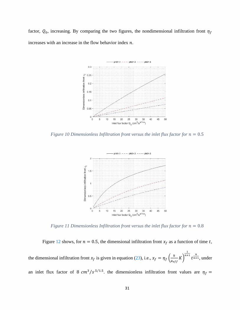
Figure 10 shows, for 𝑛 = 0.5, the non-dimensional infiltration front 휂𝑓 versus the inlet flux

factor 𝑄0, with various values of the preform porosity, for the parameters listed in Table 1, and a

well cross section area of 𝐴 = 5 𝑐𝑚2. While Figure 11 shows the results for 𝑛 = 0.8 for the same

parameters. As expected, the figures show that the infiltration front increases with the inlet flux

31

factor, 𝑄0, increasing. By comparing the two figures, the nondimensional infiltration front 휂𝑓

increases with an increase in the flow behavior index 𝑛.

Figure 10 Dimensionless Infiltration front versus the inlet flux factor for 𝑛 = 0.5


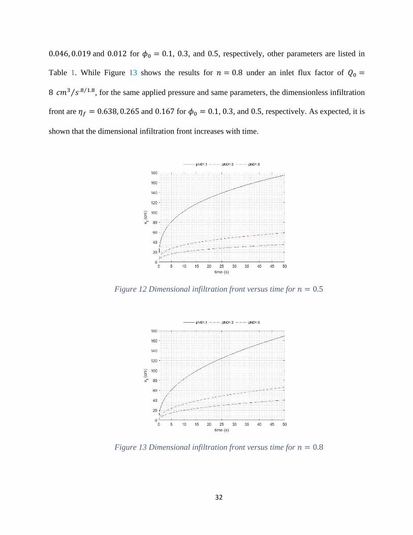
Figure 12 shows, for 𝑛 = 0.5, the dimensional infiltration front 𝑥𝑓 as a function of time 𝑡,

the dimensional infiltration front 𝑥𝑓 is given in equation (23), i.e., 𝑥𝑓 = 휂𝑓 (𝑘


1

𝑛+1𝑡

𝑛

𝑛+1, under

an inlet flux factor of 8 𝑐𝑚3 𝑠 .5 1.5⁄⁄ . the dimensionless infiltration front values are 휂𝑓 =

32

0.046, 0.019 and 0.012 for 𝜙0 = 0.1, 0.3, and 0.5, respectively, other parameters are listed in

Table 1. While Figure 13 shows the results for 𝑛 = 0.8 under an inlet flux factor of 𝑄0 =

8 𝑐𝑚3 𝑠 .8 1.8⁄⁄ , for the same applied pressure and same parameters, the dimensionless infiltration

front are 휂𝑓 = 0.638, 0.265 and 0.167 for 𝜙0 = 0.1, 0.3, and 0.5, respectively. As expected, it is

shown that the dimensional infiltration front increases with time.



33

3 ISOTHERMAL RADIAL FLOW OF A NON-NEWTONIAN FLUID IN A POROUS

MEDIUM

3.1 Basic Equations of Radial Flow

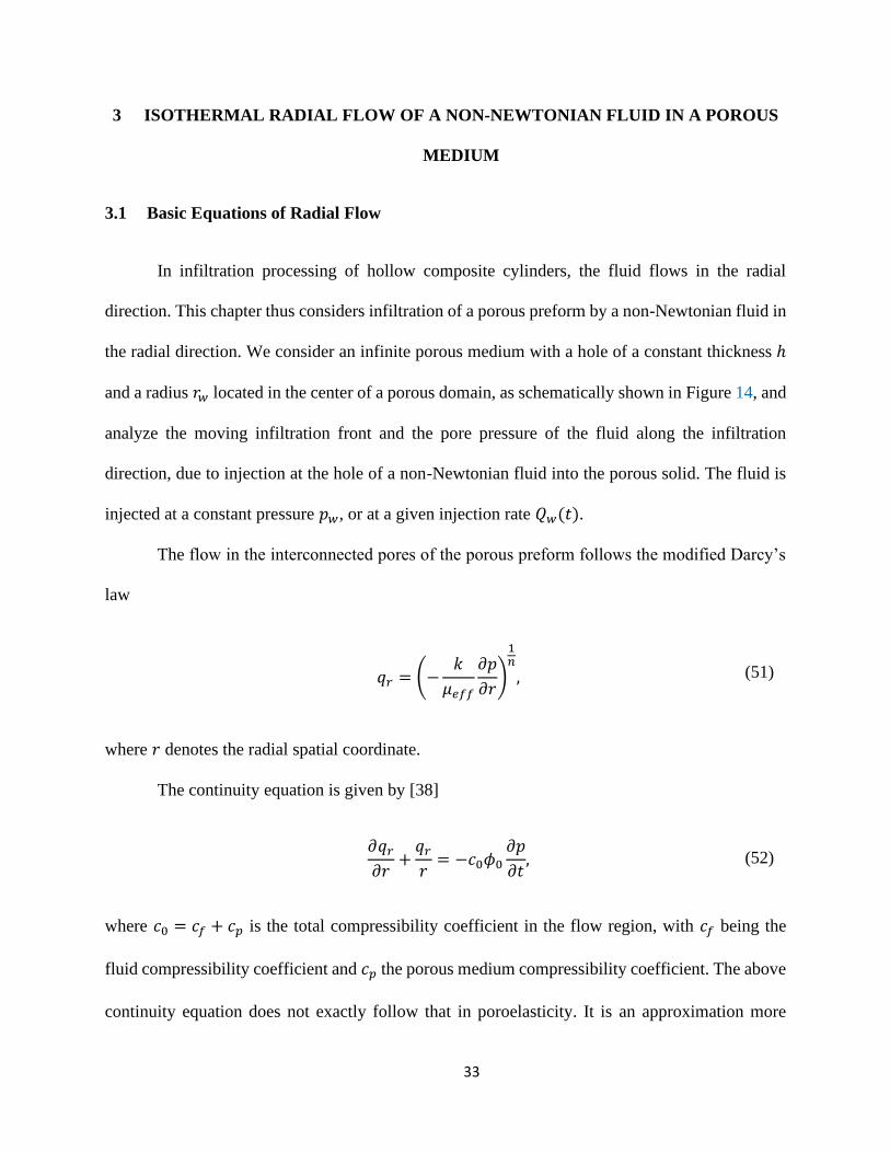
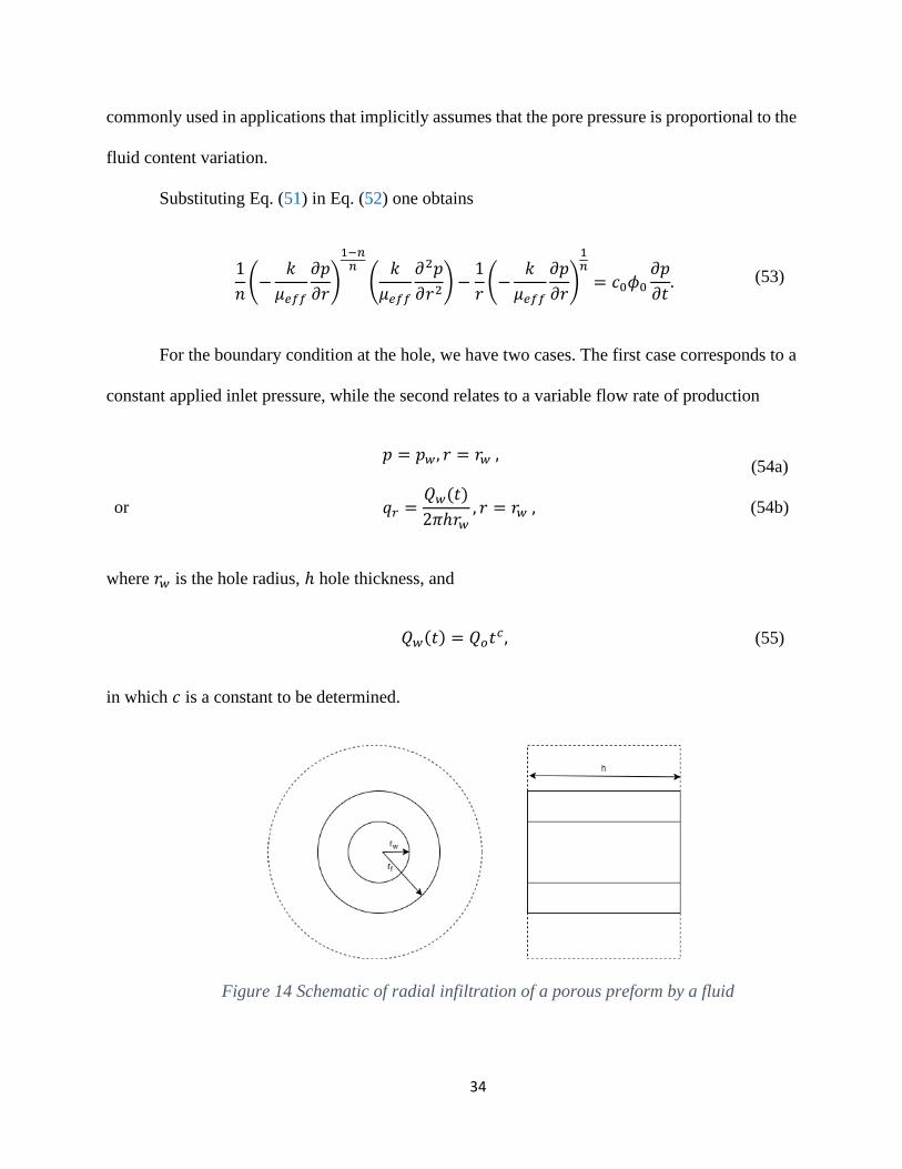
In infiltration processing of hollow composite cylinders, the fluid flows in the radial

direction. This chapter thus considers infiltration of a porous preform by a non-Newtonian fluid in

the radial direction. We consider an infinite porous medium with a hole of a constant thickness ℎ

and a radius 𝑟𝑤 located in the center of a porous domain, as schematically shown in Figure 14, and

analyze the moving infiltration front and the pore pressure of the fluid along the infiltration

direction, due to injection at the hole of a non-Newtonian fluid into the porous solid. The fluid is

injected at a constant pressure 𝑝𝑤, or at a given injection rate 𝑄𝑤(𝑡).

The flow in the interconnected pores of the porous preform follows the modified Darcy’s

law

𝑞𝑟 = (−𝑘

𝜇𝑒𝑓𝑓

𝜕𝑝

𝜕𝑟)

1𝑛

, (51)

where 𝑟 denotes the radial spatial coordinate.

The continuity equation is given by [38]

𝜕𝑞𝑟

𝜕𝑟+

𝑞𝑟

𝑟= −𝑐0𝜙0

𝜕𝑝

𝜕𝑡, (52)

where 𝑐0 = 𝑐𝑓 + 𝑐𝑝 is the total compressibility coefficient in the flow region, with 𝑐𝑓 being the

fluid compressibility coefficient and 𝑐𝑝 the porous medium compressibility coefficient. The above

continuity equation does not exactly follow that in poroelasticity. It is an approximation more

34

commonly used in applications that implicitly assumes that the pore pressure is proportional to the

fluid content variation.

Substituting Eq. (51) in Eq. (52) one obtains

1

𝑛(−

𝑘

𝜇𝑒𝑓𝑓

𝜕𝑝

𝜕𝑟)

1−𝑛𝑛

(𝑘

𝜇𝑒𝑓𝑓

𝜕2𝑝

𝜕𝑟2) −

1

𝑟(−

𝑘

𝜇𝑒𝑓𝑓

𝜕𝑝

𝜕𝑟)

1𝑛

= 𝑐0𝜙0

𝜕𝑝

𝜕𝑡. (53)

For the boundary condition at the hole, we have two cases. The first case corresponds to a

constant applied inlet pressure, while the second relates to a variable flow rate of production

or

𝑝 = 𝑝𝑤, 𝑟 = 𝑟𝑤 ,

𝑞𝑟 =𝑄𝑤(𝑡)

2𝜋ℎ𝑟𝑤, 𝑟 = 𝑟𝑤 ,

(54a)

(54b)

where 𝑟𝑤 is the hole radius, ℎ hole thickness, and

𝑄𝑤(𝑡) = 𝑄𝑜𝑡𝑐, (55)

in which 𝑐 is a constant to be determined.

Figure 14 Schematic of radial infiltration of a porous preform by a fluid

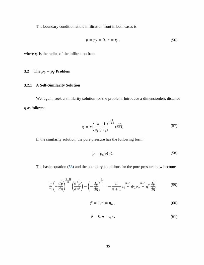
35

The boundary condition at the infiltration front in both cases is

𝑝 = 𝑝𝑓 = 0, 𝑟 = 𝑟𝑓 , (56)

where 𝑟𝑓 is the radius of the infiltration front.

3.2 The 𝒑𝟎 − 𝒑𝒇 Problem



휂 as follows:

휂 = 𝑟 (𝑘

𝜇𝑒𝑓𝑓

1

𝑐0)

−1𝑛+1

𝑡−𝑛

𝑛+1, (57)


𝑝 = 𝑝𝑤𝑝~

(휂). (58)

The basic equation (53) and the boundary conditions for the pore pressure now become

휂

𝑛(−

𝑑𝑝~

𝑑휂)

1−𝑛𝑛

(𝑑2𝑝

~

𝑑휂2) − (−

𝑑𝑝~

𝑑휂)

1𝑛

= −𝑛

𝑛 + 1𝑐0

𝑛−1𝑛 𝜙0𝑝𝑤

𝑛−1𝑛 휂2

𝑑𝑝~

𝑑휂, (59)

𝑝 = 1, 휂 = 휂𝑤 , (60)

𝑝 = 0, 휂 = 휂𝑓 , (61)

36

where 휂𝑤 is a time variable and 휂𝑓 a constants, and related respectively to the well radius 𝑟𝑤 and

infiltration front 𝑟𝑓 by

휂𝑤 = 𝑟𝑤 (𝑘

𝜇𝑒𝑓𝑓

1

𝑐0)

−1𝑛+1

𝑡−𝑛

𝑛+1, (62)

휂𝑓 = 𝑟𝑓 (𝑘

𝜇𝑒𝑓𝑓

1

𝑐0)

−1𝑛+1

𝑡−𝑛

𝑛+1. (63)

Integrating Eq. (59) yields

𝑑𝑝

~

𝑑휂= −휂−𝑛 (

𝑛2 − 𝑛

(3 − 𝑛)(1 + 𝑛)𝑐0


𝑛−1𝑛 휂3−𝑛 + 𝐶)

𝑛1−𝑛

, (64)

where 𝐶 is an integration constant, which can be expressed in terms of 휂𝑓 and 𝑝𝑤 by the infiltration

front condition

𝑑𝑟𝑓

𝑑𝑡=

1

𝜙0𝑞𝑟|𝑟=𝑟𝑓

, (65)

𝐶 = 𝑁1−𝑛휂𝑓2(1−𝑛) − 𝑀휂𝑓

3−𝑛, (66)

where 𝑀 and 𝑁 are dimensionless constants and related to the injected pressure 𝑝𝑤 by

𝑀 =𝑛2 − 𝑛

(3 − 𝑛)(1 + 𝑛)𝑐0


𝑛−1𝑛 , (67)

𝑁 =𝑛

𝑛 + 1𝑐0

−1𝑛 𝜙0𝑝𝑤

−1𝑛 , (68)

37

Now Eq. (64) becomes

𝑑𝑝

~

𝑑휂= −휂−𝑛(𝑀휂3−𝑛 − 𝑀휂𝑓

3−𝑛 + 𝑁1−𝑛휂𝑓2(1−𝑛))

𝑛1−𝑛. (69)

The solution of Eq. (69) under the boundary conditions (60) is

𝑝~

= 1 − ∫ 휂−𝑛𝜂

𝜂𝑤

(𝑀휂3−𝑛 − 𝑀휂𝑓3−𝑛 + 𝑁1−𝑛휂𝑓

2(1−𝑛))𝑛

1−𝑛𝑑휂. (70)

We may approximate 휂𝑤 ≅ 0, since 휂𝑤 < < 휂 [38]. In this case, eq (70) becomes

𝑝~

= 1 − ∫ 휂−𝑛𝜂

0


2(1−𝑛))𝑛

1−𝑛𝑑휂. (71)

Using the boundary condition (61), we obtain

∫ 휂−𝑛𝜂𝑓

0


2(1−𝑛))𝑛

1−𝑛𝑑휂 − 1 = 0. (72)

The above is the equation to determine the non-dimensional infiltration front 휂𝑓 as a

function of the applied initial pressure 𝑝𝑤.



versus the applied inlet pressure 𝑝𝑤, the dimensional infiltration front 𝑟𝑓 as a function of time 𝑡,

and the pore pressure 𝑝 along the infiltration direction 휂. Table 2 lists the poroelastic parameters

for the fluid-filled porous medium in our numerical study, which are consistent with the parameters

of the linear flow problem mentioned in the previous chapter.

38

Table 2 Poroelastic parameters for the fluid-filled porous medium

Total compressibility coefficient [𝑃𝑎−1] 𝑐0 = 1 × 10−10

Preform porosity 𝜙0 = 0.1, 0.3, 0.5

Permeability [𝑚𝐷] 𝜅 = 100

Flow behavior index 𝑛 = 0.5, 0.8

Fluid consistency index [𝑃𝑎 𝑠𝑛] 𝐻 = 0.1

The infiltration front is the most important quantity in the infiltration processing [42].

Figure 15 shows, for 𝑛 = 0.5, the non-dimensional infiltration front 휂𝑓 versus the applied inlet

fluid pressure 𝑝𝑤 with various values of the preform porosity. While Figure 16 shows the results

for 𝑛 = 0.8. It is shown that the non-dimensional infiltration front 휂𝑓 increases with an increase

in the applied inlet fluid pressure 𝑝𝑤. Comparing the results in the two figures, it is clear that

dimensionless infiltration front increases with the increase in the flow behavior index 𝑛.

Figure 15 Dimensionless infiltration front versus applied pressure for 𝑛 = 0.5

39

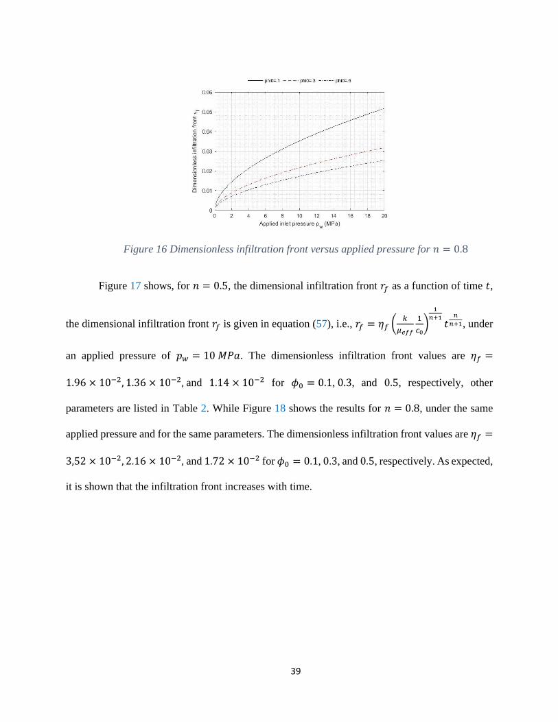
Figure 16 Dimensionless infiltration front versus applied pressure for 𝑛 = 0.8

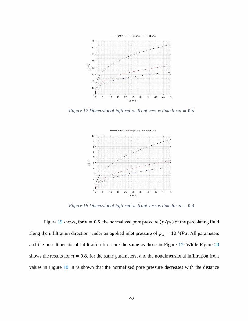
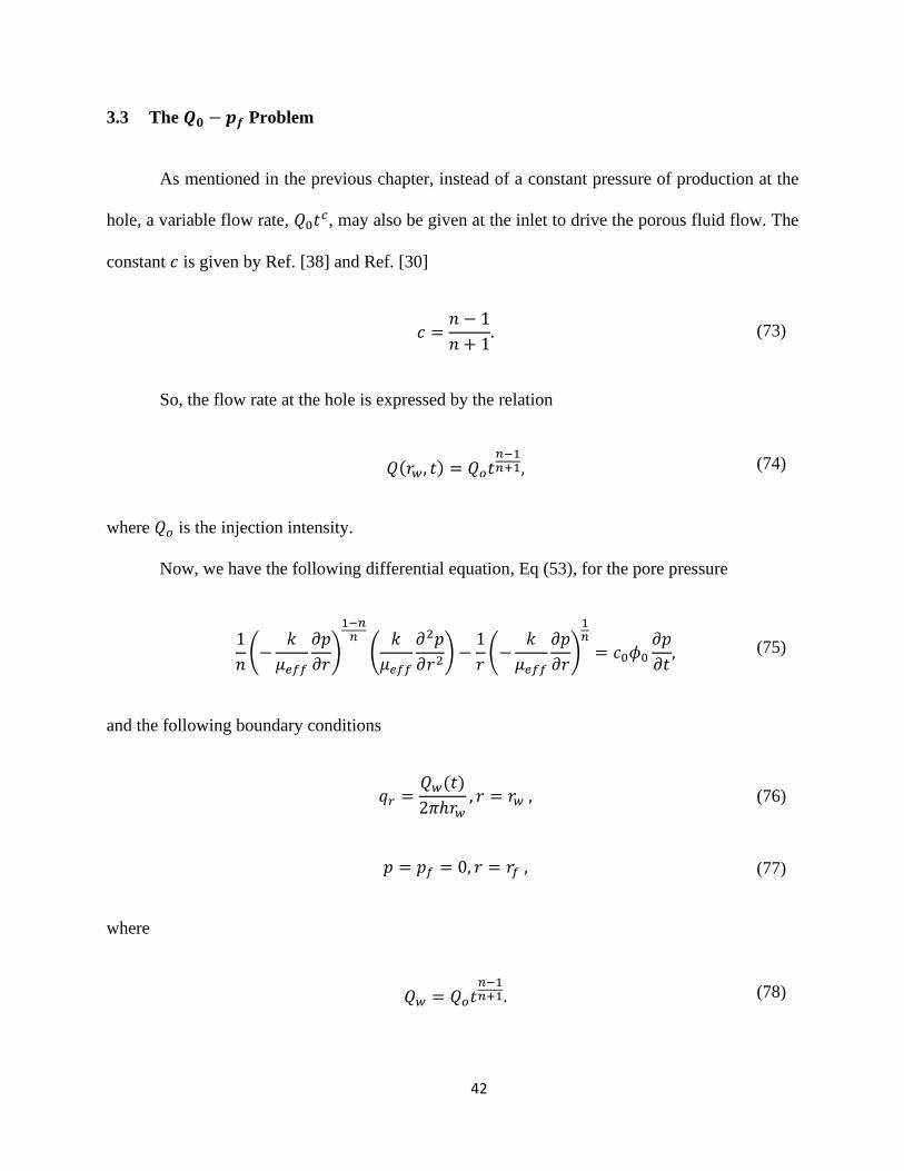
Figure 17 shows, for 𝑛 = 0.5, the dimensional infiltration front 𝑟𝑓 as a function of time 𝑡,

the dimensional infiltration front 𝑟𝑓 is given in equation (57), i.e., 𝑟𝑓 = 휂𝑓 (𝑘

𝜇𝑒𝑓𝑓

1

𝑐0)

1

𝑛+1𝑡

𝑛

𝑛+1, under

an applied pressure of 𝑝𝑤 = 10 𝑀𝑃𝑎. The dimensionless infiltration front values are 휂𝑓 =

1.96 × 10−2, 1.36 × 10−2, and 1.14 × 10−2 for 𝜙0 = 0.1, 0.3, and 0.5, respectively, other

parameters are listed in Table 2. While Figure 18 shows the results for 𝑛 = 0.8, under the same

applied pressure and for the same parameters. The dimensionless infiltration front values are 휂𝑓 =

3,52 × 10−2, 2.16 × 10−2, and 1.72 × 10−2 for 𝜙0 = 0.1, 0.3, and 0.5, respectively. As expected,

it is shown that the infiltration front increases with time.

40



Figure 19 shows, for 𝑛 = 0.5, the normalized pore pressure (𝑝 𝑝0⁄ ) of the percolating fluid

along the infiltration direction. under an applied inlet pressure of 𝑝𝑤 = 10 𝑀𝑃𝑎. All parameters

and the non-dimensional infiltration front are the same as those in Figure 17. While Figure 20

shows the results for 𝑛 = 0.8, for the same parameters, and the nondimensional infiltration front

values in Figure 18. It is shown that the normalized pore pressure decreases with the distance

41

increasing from the inlet and drops to zero at the infiltration front, where the fluid stops moving.

The pressure distribution is not linear.


Figure 20Normalized pore pressure along the infiltration direction for 𝑛 = 0.8

42

3.3 The 𝑸𝟎 − 𝒑𝒇 Problem

As mentioned in the previous chapter, instead of a constant pressure of production at the

hole, a variable flow rate, 𝑄0𝑡𝑐, may also be given at the inlet to drive the porous fluid flow. The

constant 𝑐 is given by Ref. [38] and Ref. [30]

𝑐 =𝑛 − 1

𝑛 + 1. (73)

So, the flow rate at the hole is expressed by the relation

𝑄(𝑟𝑤, 𝑡) = 𝑄𝑜𝑡𝑛−1𝑛+1, (74)

where 𝑄𝑜 is the injection intensity.

Now, we have the following differential equation, Eq (53), for the pore pressure

1

𝑛(−

𝑘

𝜇𝑒𝑓𝑓

𝜕𝑝

𝜕𝑟)

1−𝑛𝑛

(𝑘

𝜇𝑒𝑓𝑓

𝜕2𝑝

𝜕𝑟2) −

1

𝑟(−

𝑘

𝜇𝑒𝑓𝑓

𝜕𝑝

𝜕𝑟)

1𝑛

= 𝑐0𝜙0

𝜕𝑝

𝜕𝑡, (75)

and the following boundary conditions


2𝜋ℎ𝑟𝑤, 𝑟 = 𝑟𝑤 , (76)

𝑝 = 𝑝𝑓 = 0, 𝑟 = 𝑟𝑓 , (77)

where

𝑄𝑤 = 𝑄𝑜𝑡𝑛−1𝑛+1. (78)

43



휂 as follows:

휂 = 𝑟 (𝑘

𝜇𝑒𝑓𝑓

1

𝑐0)

−1𝑛+1

𝑡−𝑛

𝑛+1. (79)


𝑝(𝑥, 𝑡) = 𝐷𝑄𝑤�̃�(휂), (80)

where 𝐷 [𝑀𝐿−4𝑇−1] is a constant, and 𝑝 is the nondimensional pore pressure and is a function of

휂 only.

Using the dimensionless variables, the basic equation (75) and the boundary conditions for

the pore pressure now become

휂

𝑛(−

𝑑𝑝~

𝑑휂)

1−𝑛𝑛

(𝑑2𝑝

~

𝑑휂2) − (−

𝑑𝑝~

𝑑휂)

1𝑛

= −𝑛

𝑛 + 1𝑐0

𝑛−1𝑛 𝜙0(𝐷𝑄𝑤)

𝑛−1𝑛 휂2

𝑑𝑝~

𝑑휂, (81)


2𝜋ℎ𝑟𝑤, 휂 = 휂𝑤 , (82)

𝑝 = 0, 휂 = 휂𝑓 . (83)

Integrating Eq. (81), we get

𝑑𝑝

~

𝑑휂= −휂−𝑛 (

𝑛2 − 𝑛

(3 − 𝑛)(1 + 𝑛)𝑐0

𝑛−1𝑛 𝜙0(𝐷𝑄𝑤)

𝑛−1𝑛 휂3−𝑛 + 𝐶0)

𝑛1−𝑛

, (84)

44

where 𝐶0 is an integration constant. Using the infiltration front condition

𝑑𝑟𝑓

𝑑𝑡=

1

𝜙0𝑞𝑟|𝑟=𝑟𝑓

, (85)

the constant 𝐶0 can be determined as follows:

𝐶0 = (𝑉1−𝑛휂𝑓2(1−𝑛) − 𝑊휂𝑓

3−𝑛)(𝐷𝑄𝑤)𝑛−1

𝑛 , (86)

where 𝑊 and 𝑉 are constants given by

𝑊 =𝑛2 − 𝑛

(3 − 𝑛)(1 + 𝑛)𝑐0

𝑛−1𝑛 𝜙0 , (87)

𝑉 =𝑛

𝑛 + 1𝑐0

−1𝑛 𝜙0 . (88)

Now Eq. (84) becomes

𝑑𝑝

~

𝑑휂= −휂−𝑛(𝑊휂3−𝑛 − 𝑊휂𝑓

3−𝑛 + 𝑉1−𝑛휂𝑓2(1−𝑛))

𝑛1−𝑛(𝐷𝑄𝑤)−1. (89)

Using the boundary condition (82), and Eqs. (74), (89) and (51), we obtain the following

equation

𝑄𝑜

2𝜋ℎ= (

𝑘

𝜇𝑒𝑓𝑓)

2𝑛+1𝑐0

1−𝑛𝑛2+𝑛(𝑊휂𝑤

3−𝑛 − 𝑊휂𝑓3−𝑛 + 𝑉1−𝑛휂𝑓

2(1−𝑛))1

1−𝑛. (90)

Since the well radius 𝑟𝑤 is very small, 휂𝑤 < < 휂, we may approximate 휂𝑤 ≅ 0. In this

case, Eq. (90) becomes

𝑄𝑜

2𝜋ℎ= (

𝑘

𝜇𝑒𝑓𝑓)

2𝑛+1𝑐0

1−𝑛𝑛2+𝑛(−𝑊휂𝑓

3−𝑛 + 𝑉1−𝑛휂𝑓2(1−𝑛))

11−𝑛. (91)

45

The above equation is used to determine the non-dimensional infiltration front 휂𝑓 in terms

of the flow-rate factor 𝑄𝑜



versus the inlet flux factor 𝑄𝑜, and the dimensional infiltration front 𝑟𝑓 as a function of time 𝑡.

Table 2 lists the poroelastic parameters for the fluid-filled porous medium in our numerical

calculations.

As mentioned earlier, the infiltration front is the most important quantity in the infiltration

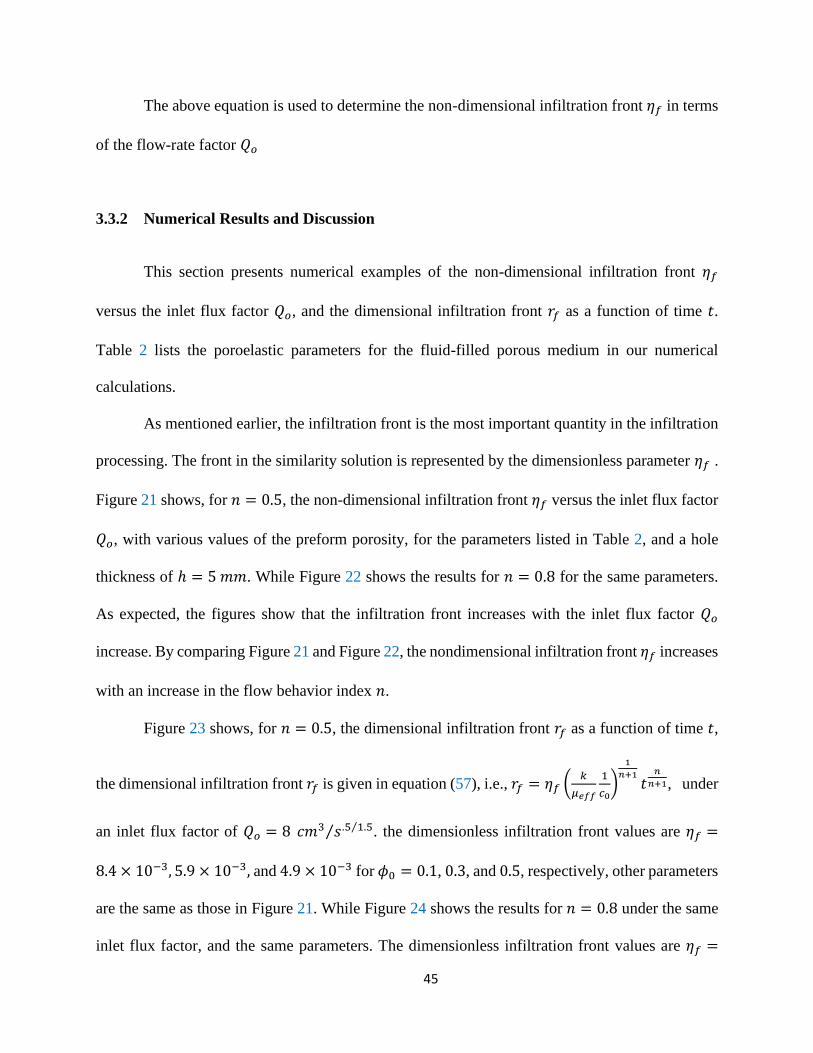
processing. The front in the similarity solution is represented by the dimensionless parameter 휂𝑓 .

Figure 21 shows, for 𝑛 = 0.5, the non-dimensional infiltration front 휂𝑓 versus the inlet flux factor

𝑄𝑜, with various values of the preform porosity, for the parameters listed in Table 2, and a hole

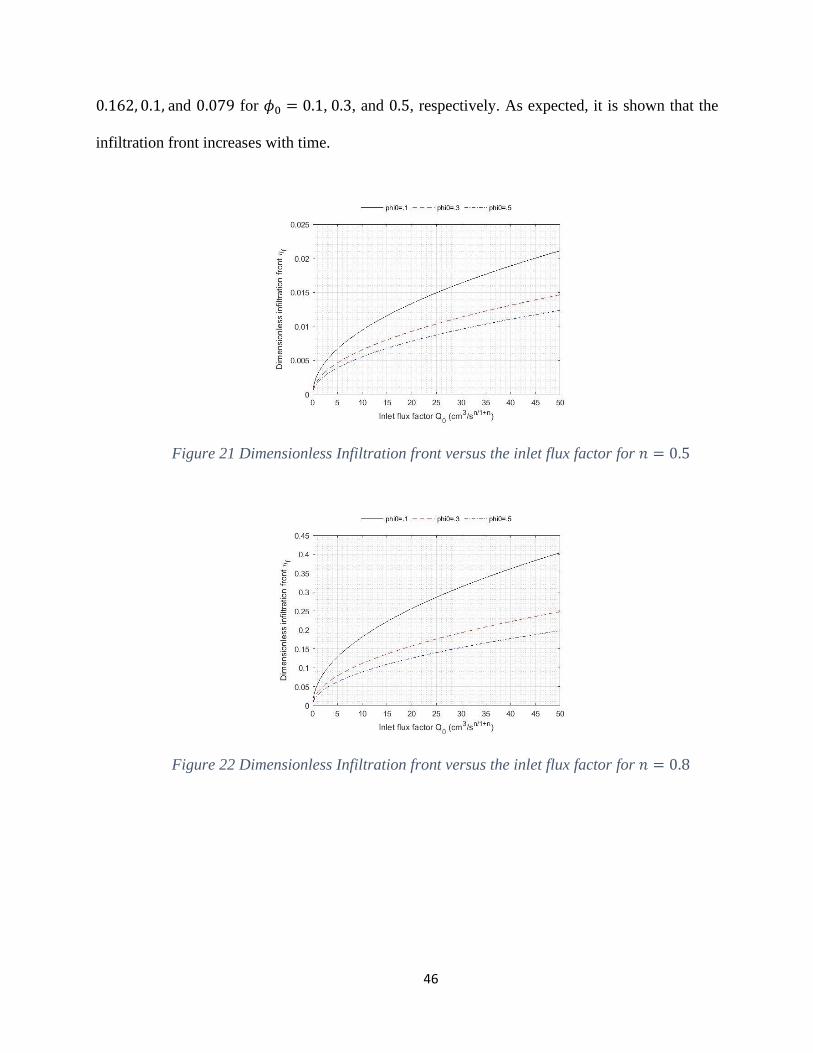
thickness of ℎ = 5 𝑚𝑚. While Figure 22 shows the results for 𝑛 = 0.8 for the same parameters.

As expected, the figures show that the infiltration front increases with the inlet flux factor 𝑄𝑜

increase. By comparing Figure 21 and Figure 22, the nondimensional infiltration front 휂𝑓 increases

with an increase in the flow behavior index 𝑛.

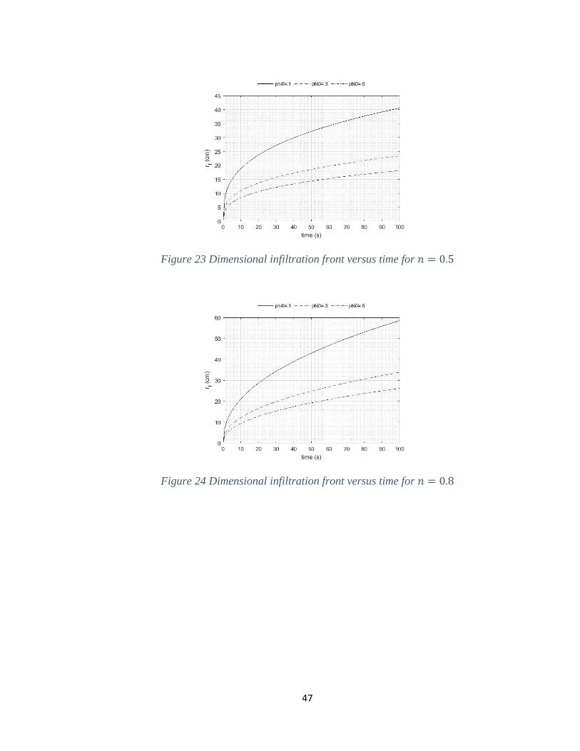
Figure 23 shows, for 𝑛 = 0.5, the dimensional infiltration front 𝑟𝑓 as a function of time 𝑡,

the dimensional infiltration front 𝑟𝑓 is given in equation (57), i.e., 𝑟𝑓 = 휂𝑓 (𝑘

𝜇𝑒𝑓𝑓

1

𝑐0)

1

𝑛+1𝑡

𝑛

𝑛+1, under

an inlet flux factor of 𝑄𝑜 = 8 𝑐𝑚3 𝑠 .5 1.5⁄⁄ . the dimensionless infiltration front values are 휂𝑓 =

8.4 × 10−3, 5.9 × 10−3, and 4.9 × 10−3 for 𝜙0 = 0.1, 0.3, and 0.5, respectively, other parameters

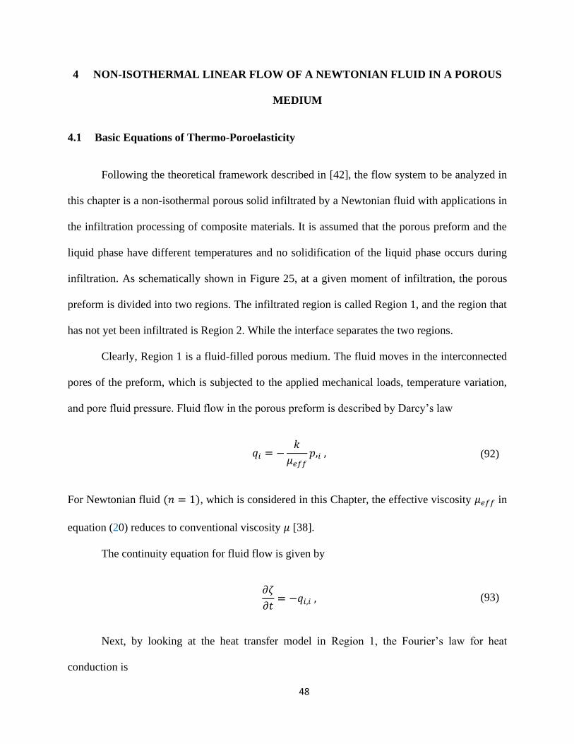
are the same as those in Figure 21. While Figure 24 shows the results for 𝑛 = 0.8 under the same

inlet flux factor, and the same parameters. The dimensionless infiltration front values are 휂𝑓 =

46

0.162, 0.1, and 0.079 for 𝜙0 = 0.1, 0.3, and 0.5, respectively. As expected, it is shown that the

infiltration front increases with time.



47



48

4 NON-ISOTHERMAL LINEAR FLOW OF A NEWTONIAN FLUID IN A POROUS

MEDIUM

4.1 Basic Equations of Thermo-Poroelasticity

Following the theoretical framework described in [42], the flow system to be analyzed in

this chapter is a non-isothermal porous solid infiltrated by a Newtonian fluid with applications in

the infiltration processing of composite materials. It is assumed that the porous preform and the

liquid phase have different temperatures and no solidification of the liquid phase occurs during

infiltration. As schematically shown in Figure 25, at a given moment of infiltration, the porous

preform is divided into two regions. The infiltrated region is called Region 1, and the region that

has not yet been infiltrated is Region 2. While the interface separates the two regions.

Clearly, Region 1 is a fluid-filled porous medium. The fluid moves in the interconnected

pores of the preform, which is subjected to the applied mechanical loads, temperature variation,

and pore fluid pressure. Fluid flow in the porous preform is described by Darcy’s law

𝑞𝑖 = −𝑘

𝜇𝑒𝑓𝑓𝑝,𝑖 , (92)

For Newtonian fluid (𝑛 = 1), which is considered in this Chapter, the effective viscosity 𝜇𝑒𝑓𝑓 in

equation (20) reduces to conventional viscosity 𝜇 [38].

The continuity equation for fluid flow is given by

𝜕휁

𝜕𝑡= −𝑞𝑖,𝑖 , (93)

Next, by looking at the heat transfer model in Region 1, the Fourier’s law for heat

conduction is

49

ℎ𝑖 = −𝜆1휃,𝑖 , (94)

where ℎ𝑖 is the heat flux vector, 휃 is the temperature variation, and 𝜆1 is the thermal conductivity

of the fluid-filled porous medium in Region 1. The temperature is governed by the heat conduction

equation

𝜌1𝑐1

𝜕휃

𝜕𝑡= 𝜆1∇2휃 + 𝑞𝑓𝑠 , (95)

where 𝜌1 and 𝑐1 are the mass density and specific heat of the fluid-filled porous medium in Region-

1, respectively, ∇2 the Laplacian operator. and 𝑞𝑓𝑠 accounts for the convection induced heat

transfer and is given by

𝑞𝑓𝑠 = −𝜌𝑓𝑐𝑓𝑞𝑖휃,𝑖 , (96)

where 𝜌𝑓 and 𝑐𝑓 are the mass density and specific heat of the fluid, respectively.

Substituting equation (96) into equation (95), we get

𝜌1𝑐1

𝜕휃

𝜕𝑡+ 𝜌𝑓𝑐𝑓𝑞𝑖휃,𝑖 = 𝜆1∇2휃. (97)

In thermo-poroelasticity, the constitutive equations are [52]

𝜎𝑖𝑗 = 2𝐺휀𝑖𝑗 +2𝐺𝜐

1 − 2𝜐휀𝑘𝑘𝛿𝑖𝑗 − 𝛼𝑝𝛿𝑖𝑗 − 𝐾𝛼𝑠휃𝛿𝑖𝑗 , (98)

휁 =𝛼

3𝐾(𝜎𝑘𝑘 +

3𝑝

𝐵) − 𝜙0(𝛼𝑓 − 𝛼𝑠)휃, (99)

where 𝛼𝑠 is the volumetric thermal expansion coefficient of the preform, and 𝛼𝑓 the volumetric

thermal expansion coefficient of the fluid.

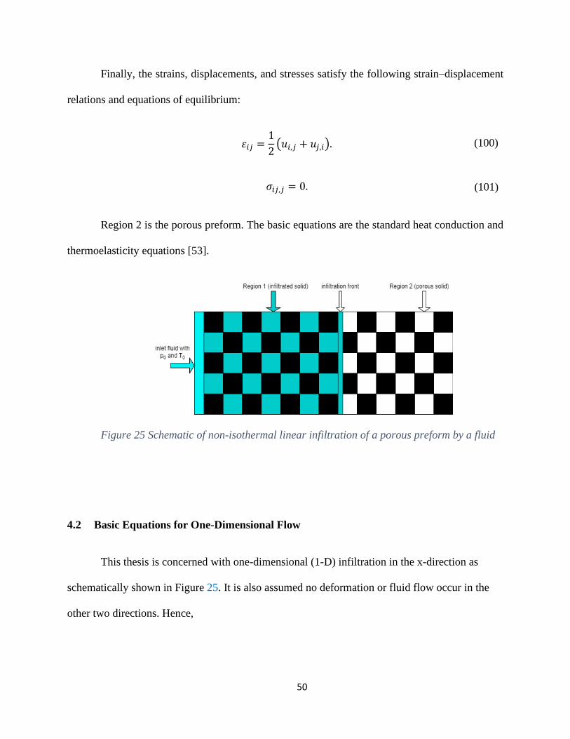
50

Finally, the strains, displacements, and stresses satisfy the following strain–displacement

relations and equations of equilibrium:

휀𝑖𝑗 =1

2(𝑢𝑖,𝑗 + 𝑢𝑗,𝑖). (100)

𝜎𝑖𝑗,𝑗 = 0. (101)

Region 2 is the porous preform. The basic equations are the standard heat conduction and

thermoelasticity equations [53].

Figure 25 Schematic of non-isothermal linear infiltration of a porous preform by a fluid

4.2 Basic Equations for One-Dimensional Flow

This thesis is concerned with one-dimensional (1-D) infiltration in the x-direction as

schematically shown in Figure 25. It is also assumed no deformation or fluid flow occur in the

other two directions. Hence,

51

𝑢𝑦 = 𝑢𝑧 = 0,

휀𝑦𝑦 = 휀𝑧𝑧 = 휀𝑥𝑦 = 휀𝑦𝑧 = 휀𝑥𝑦 = 0,

(102a)

(102b)

𝑞𝑦 = 𝑞𝑧 = 0. (103)

Now all field variables are functions of 𝑥 and time 𝑡, for example, the temperature variation is 휃 =

휃(𝑥, 𝑡).

The boundary conditions for the problem are

𝑝 = 𝑝0, 𝑥 = 0,

(104)

𝑝 = 0, 𝑥 = 𝑥𝑓 ,

(105)

𝜎𝑥𝑥 = −𝑝0, 𝑥 = 0,

(106)

휃 = 휃0, 𝑥 = 0,

(107)

where 휃0 is the inlet temperature.

Now the equilibrium equation (101) reduces to Eq. (13) in Chapter 2, i.e.,

𝜎𝑥𝑥,𝑥 = 0,

(108)

which means the normal stress 𝜎𝑥𝑥 is a constant. Using the boundary condition (106), we get

𝜎𝑥𝑥 = −𝑝0, 0 ≤ 𝑥 ≤ 𝑥𝑓 .

(109)

4.2.1 Region 1 (𝟎 < 𝒙 < 𝒙𝒇)

Under the above 1-D isothermal infiltration conditions, Darcy’s law reduces to

𝑞𝑥 = −𝜅𝜕𝑝

𝜕𝑥. (110)

52

The normal stresses and strain for the 1D infiltration can be deduced from Eqs. (98), (102a)

(102b) and the boundary condition (106) as follows:

𝜎𝑦𝑦 = 𝜎𝑧𝑧 = −𝜐

1 − 𝜐𝑝0 −

1 − 2𝜐

1 − 𝜐(𝛼𝑝 + 𝐾𝛼𝑠휃1), (111)

휀𝑥𝑥 =1 + 𝜐

3(1 − 𝜐)𝐾(−𝑝0 + 𝛼𝑝𝐾𝛼𝑠휃1) (112)

where 휃1 the temperature variation in Region 1. Now the governing equations for the temperature

variation, pore pressure, and liquid content variation reduce to

𝜕휃1

𝜕𝑡−

𝜌𝑓𝑐𝑓

𝜌1𝑐1𝜅

𝜕𝑝

𝜕𝑥

𝜕휃1

𝜕𝑥− 𝜅1

𝜕2휃1

𝜕𝑥2= 0,

(113)

𝜕𝑝

𝜕𝑡= 𝜅

𝐾

�̃�

𝜕2𝑝

𝜕𝑥2+

𝐾𝜔𝛼𝑠

�̃�

𝜕휃1

𝜕𝑡, (114)

휁 =�̃�

𝐾𝑝 − 𝜔𝛼2휃1 −

𝛼

3𝐾

1 + 𝜐

1 − 𝜐𝑝0 , (115)

where 𝜔 is a dimensionless parameter given by

𝜔 =2(1 − 2𝜐)

3(1 − 𝜐)𝛼 + 𝜙0

𝛼𝑓 − 𝛼𝑠

𝛼𝑠, (116)

and 𝜅1 is the thermal diffusivity of the porous preform, and given by the equation

𝜅1 = 𝜆1 (𝜌1𝑐1)⁄ , (117)

in which 𝜆1 is the thermal conductivity, 𝜌1 the density, and 𝑐1 the specific heat of the porous

preform, respectively.

53

4.2.2 Region 2 (𝒙 > 𝒙𝒇)

Region 2 is the porous preform. The temperature variation field is governed by the standard

heat equation, i.e.,

𝜕휃2

𝜕𝑡= 𝜅2

𝜕2휃2

𝜕𝑥2, (118)

where 𝜅2 is the thermal diffusivity of the porous preform

𝜅2 = 𝜆2 (𝜌2𝑐2),⁄ (119)

where 𝜆2 is the thermal conductivity, 𝜌2 the density, and 𝑐2 the specific heat of the porous preform,

respectively.

Boundary conditions for the temperature variation at the interface between Regions 1 and

2, i.e., the infiltration front, are deduced from the temperature and heat flux continuity conditions

as follows:

휃1(𝑥𝑓 , 𝑡) = 휃2(𝑥𝑓 , 𝑡), 𝑡 > 0, (120)

𝜆1

𝜕휃1

𝜕𝑥(𝑥𝑓 , 𝑡) = 𝜆2

𝜕휃2

𝜕𝑥(𝑥𝑓 , 𝑡), 𝑡 > 0. (121)

The temperature 휃2 goes to the initial temperature of the preform at distances far from the

infiltration front. We thus have the third boundary condition as follows:

휃2 → 0, 𝑥 → ∞. (122)

54

4.3 A Self-Similarity Solution

Again, we seek a similarity solution for the non-isothermal infiltration problem. Introduce

a dimensionless distance 휂 as follows:

휂 = 𝑥 √𝑘

𝜇𝐾𝑡⁄ . (123)

In the similarity solution, the pore pressure, temperature variation in Region1, and

temperature variation in Region 2 have the following forms:

𝑝(𝑥, 𝑡) = 𝑝0𝑝(휂). (124)

휃1(𝑥, 𝑡) = 𝑇0휃̃1(휂). (125)

휃2(𝑥, 𝑡) = 𝑇0휃̃2(휂). (126)

Under the self-similar infiltration conditions, Eqs. (113) and (114) for Region 1 become

[42]

𝑑2휃̃1

𝑑휂2+

1

2𝜅1

𝑘𝐾

𝜇휂

𝑑휃̃1

𝑑휂+

𝜌𝑓𝑐𝑓𝑝0

𝜆1

𝑘

𝜇

𝑑𝑝

𝑑휂

𝑑휃̃1

𝑑휂= 0. (127)

𝑑2𝑝

𝑑휂2+

1

2�̃�휂

𝑑𝑝

𝑑휂−

𝐾𝜔𝛼𝑠𝑇0

2𝑝0휂

𝑑휃̃1

𝑑휂= 0. (128)

Clearly the temperature and pore pressure in Region 1 are coupled together due to the

convective heat transfer. Moreover, the equations are nonlinear. The convection term was

neglected in the solution in [42]. The boundary conditions for the normalized temperature and pore

pressure are

55

휃̃1(0) = 휃0 𝑇0⁄ . (129)

휃̃1(휂𝑓) = 휃̃2(휂𝑓). (130)

𝜆1

𝑑휃̃1

𝑑휂(휂𝑓) = 𝜆2

𝑑휃̃2

𝑑휂(휂𝑓). (131)

𝑝(0) = 1. (132)

𝑝(휂𝑓) = 0. (133)

In Region 2, the governing equation for the temperature, Eq. (118), becomes

𝑑2휃̃2

𝑑휂2+

1

2𝜅2

𝑘𝐾

𝜇휂

𝑑휃̃2

𝑑휂= 0. (134)

Integrating the above equation yields

𝑑휃̃2

𝑑휂= 𝐷1𝑒

−1

2𝜅2

𝑘𝐾𝜇

𝜂2

2 , (135)

where 𝐷1 ≠ 𝐷1(휂, 휃̃2) is a constant to be determined. The solution of the above equation is

휃̃2 = 𝐷1√𝜋𝜇𝜅2

𝑘𝐾[erf (√

𝑘𝐾

𝜇

휂

2√𝜅2

) − 1]. (136)

Using the above temperature expressions in Region 2, the continuity conditions in

Equations (130) and (131) become

56

휃̃1(휂𝑓) = 𝐷1√𝜋𝜇𝜅2

𝑘𝐾[erf (√

𝑘𝐾

𝜇

휂𝑓

2√𝜅2

) − 1], (137)

𝑑휃̃1

𝑑휂(휂𝑓) =

𝜆2

𝜆1𝐷1𝑒

−1

2𝜅2

𝑘𝐾𝜇

𝜂𝑓2

2 . (138)

4.4 Numerical Results and Discussion

This section presents the numerical examples of the non-dimensional infiltration front 휂𝑓

versus the applied inlet pressure 𝑝0, the dimensional infiltration front 𝑥𝑓 as a function of time 𝑡,

the pore pressure 𝑝 along the infiltration direction 휂, the temperature distribution 휃 along the

infiltration direction 휂, and the normalized liquid content variation 휁 (𝑝0 𝐾⁄ )⁄ along the infiltration

direction 휂 during the infiltration of a ceramic preform by a liquid polymer with the same

properties used in [42], which are possible for dental applications [42]. Table 1 lists the poroelastic

parameters for the fluid-filled porous medium in the numerical calculations and Table 3 lists the

thermal properties of the fluid and solid phases.

The specific heat capacity and density for the fluid-filled porous solid in Region 1 is

determined using the following rule of mixtures [42]:

𝜌1 = 𝜙0𝜌𝑓 + (1 − 𝜙0)𝜌𝑠, (139)

𝑐1 = 𝜙0𝑐𝑓 + (1 − 𝜙0)𝑐𝑠, (140)

57

subscripts 𝑓 and 𝑠 denote the properties of the fluid and solid phases, respectively, and the porosity

is the volume fraction of the fluid phase. The thermal conductivity in Region 1 is determined using

a matricity-based model for interpenetrating phase composites as follows [54]:

𝑘1 = 𝑘𝐼𝐼 +(𝑘𝐼 − 𝑘𝐼𝐼)𝑀𝛼

(1 − 𝑟) + 𝑟(𝑀𝛼 + 𝑀𝛽 𝑘𝐼 𝑘𝐼𝐼⁄ ), (141)

where 𝑘𝐼 and 𝑘𝐼𝐼 are the thermal conductivities of αM (solid as matrix) and βM (fluid as matrix)

phases and are determined using the models of the Hashin-Shtrikman [55]

𝑘𝐼 = 𝑘𝛼 {1 +(1 − 𝜙0)(𝑘𝛽 − 𝑘𝛼)

𝑘𝛼 + (𝑘𝛽 − 𝑘𝛼) 𝜙0 3⁄}, (142)

𝑘𝐼𝐼 = 𝑘𝛽 {1 +(1 − 𝜙0)(𝑘𝛼 − 𝑘𝛽)

𝑘𝛽 + (𝑘𝛼 − 𝑘𝛽) 𝜙0 3⁄}, (143)

where 𝑘𝛼 and 𝑘𝛽 are the thermal conductivities of the α-phase (fluid) and β-phase (solid),

respectively. The matricities Mα and Mβ describe the connectivity of the α-phase (fluid) and β-

phase (solid) in the fluid-filled preform, respectively. Because both the solid and fluid are fully

interconnected, the matricities are taken as 0.5. Moreover, parameter r is also taken as 0.5 in the

calculation as it does not significantly influence the thermal conductivity. While the same

properties in Region 2 are determined by the same methods by taking the properties of the air,

instead of the liquid, as the 𝛼- phase.

The nonlinear equations (127) and (128) are solved numerically using the Runge-Kutta 4th

order method. To solve for 휂𝑓(𝑝0), and 𝐷1(𝑝0), the unknowns in the boundary conditions, the 2

coupled differential equations with the 5 boundary conditions and the infiltration front velocity

boundary condition, Eq. (32), are solved firstly at some specific points of 𝑝0 using trial and error

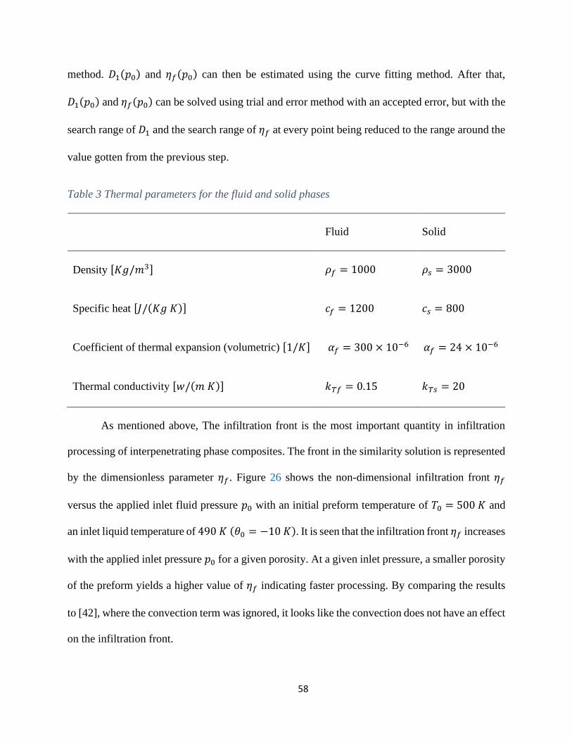
58

method. 𝐷1(𝑝0) and 휂𝑓(𝑝0) can then be estimated using the curve fitting method. After that,

𝐷1(𝑝0) and 휂𝑓(𝑝0) can be solved using trial and error method with an accepted error, but with the

search range of 𝐷1 and the search range of 휂𝑓 at every point being reduced to the range around the

value gotten from the previous step.

Table 3 Thermal parameters for the fluid and solid phases

Fluid Solid

Density [𝐾𝑔/𝑚3] 𝜌𝑓 = 1000 𝜌𝑠 = 3000

Specific heat [𝐽/(𝐾𝑔 𝐾)] 𝑐𝑓 = 1200 𝑐𝑠 = 800

Coefficient of thermal expansion (volumetric) [1/𝐾] 𝛼𝑓 = 300 × 10−6 𝛼𝑓 = 24 × 10−6

Thermal conductivity [𝑤/(𝑚 𝐾)] 𝑘𝑇𝑓 = 0.15 𝑘𝑇𝑠 = 20

As mentioned above, The infiltration front is the most important quantity in infiltration

processing of interpenetrating phase composites. The front in the similarity solution is represented

by the dimensionless parameter 휂𝑓. Figure 26 shows the non-dimensional infiltration front 휂𝑓

versus the applied inlet fluid pressure 𝑝0 with an initial preform temperature of 𝑇0 = 500 𝐾 and

an inlet liquid temperature of 490 𝐾 (휃0 = −10 𝐾). It is seen that the infiltration front 휂𝑓 increases

with the applied inlet pressure 𝑝0 for a given porosity. At a given inlet pressure, a smaller porosity

of the preform yields a higher value of 휂𝑓 indicating faster processing. By comparing the results

to [42], where the convection term was ignored, it looks like the convection does not have an effect

on the infiltration front.

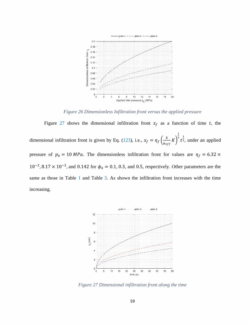
59

Figure 26 Dimensionless Infiltration front versus the applied pressure

Figure 27 shows the dimensional infiltration front 𝑥𝑓 as a function of time 𝑡, the

dimensional infiltration front is given by Eq. (123), i.e., 𝑥𝑓 = 휂𝑓 (𝑘


1

2𝑡

1

2, under an applied

pressure of 𝑝0 = 10 𝑀𝑃𝑎. The dimensionless infiltration front for values are 휂𝑓 = 6.32 ×

10−2, 8.17 × 10−2, and 0.142 for 𝜙0 = 0.1, 0.3, and 0.5, respectively. Other parameters are the

same as those in Table 1 and Table 3. As shown the infiltration front increases with the time

increasing.

Figure 27 Dimensional infiltration front along the time

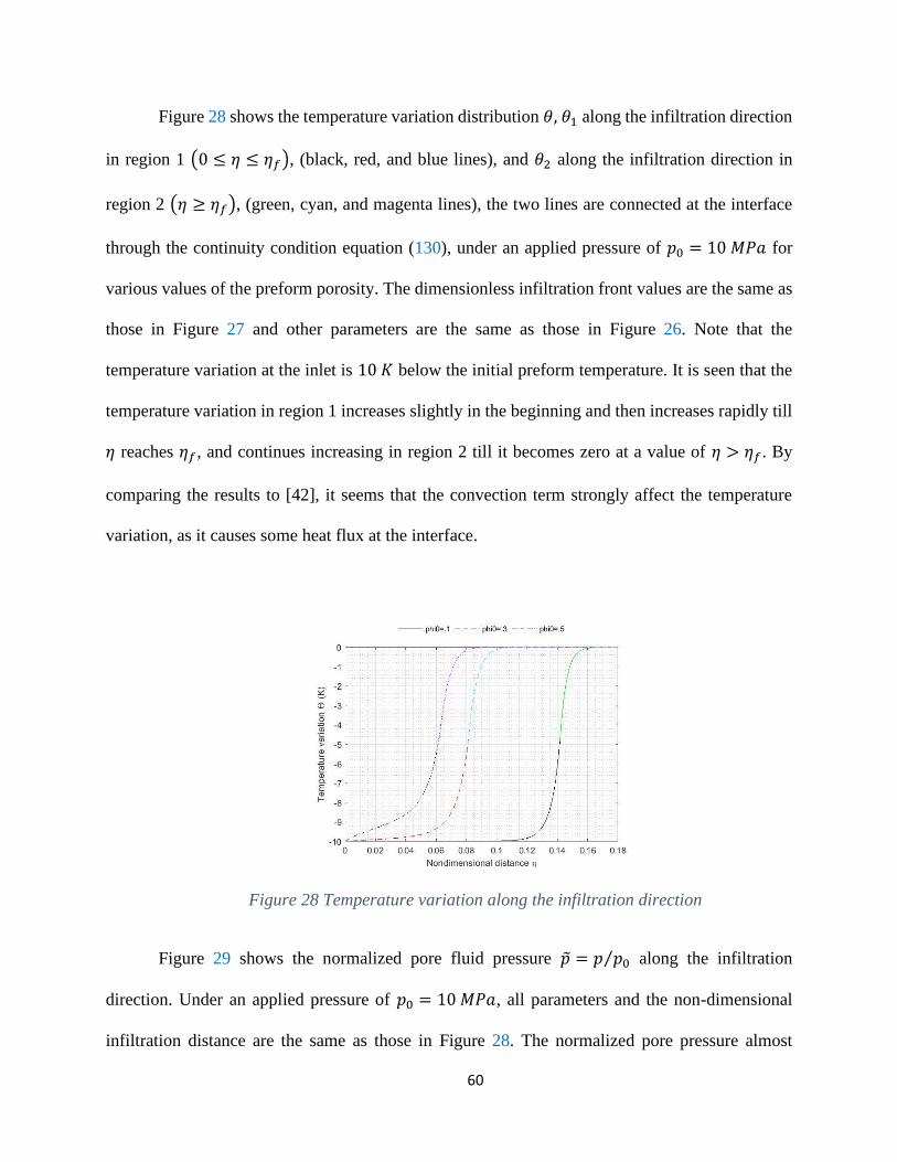
60

Figure 28 shows the temperature variation distribution 휃, 휃1 along the infiltration direction

in region 1 (0 ≤ 휂 ≤ 휂𝑓), (black, red, and blue lines), and 휃2 along the infiltration direction in

region 2 (휂 ≥ 휂𝑓), (green, cyan, and magenta lines), the two lines are connected at the interface

through the continuity condition equation (130), under an applied pressure of 𝑝0 = 10 𝑀𝑃𝑎 for

various values of the preform porosity. The dimensionless infiltration front values are the same as

those in Figure 27 and other parameters are the same as those in Figure 26. Note that the

temperature variation at the inlet is 10 𝐾 below the initial preform temperature. It is seen that the

temperature variation in region 1 increases slightly in the beginning and then increases rapidly till

휂 reaches 휂𝑓, and continues increasing in region 2 till it becomes zero at a value of 휂 > 휂𝑓. By

comparing the results to [42], it seems that the convection term strongly affect the temperature

variation, as it causes some heat flux at the interface.

Figure 28 Temperature variation along the infiltration direction

Figure 29 shows the normalized pore fluid pressure 𝑝 = 𝑝 𝑝0⁄ along the infiltration

direction. Under an applied pressure of 𝑝0 = 10 𝑀𝑃𝑎, all parameters and the non-dimensional

infiltration distance are the same as those in Figure 28. The normalized pore pressure almost

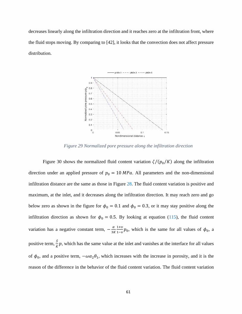
61

decreases linearly along the infiltration direction and it reaches zero at the infiltration front, where

the fluid stops moving. By comparing to [42], it looks that the convection does not affect pressure

distribution.

Figure 29 Normalized pore pressure along the infiltration direction

Figure 30 shows the normalized fluid content variation 휁 (𝑝0 𝐾⁄ )⁄ along the infiltration

direction under an applied pressure of 𝑝0 = 10 𝑀𝑃𝑎. All parameters and the non-dimensional

infiltration distance are the same as those in Figure 28. The fluid content variation is positive and

maximum, at the inlet, and it decreases along the infiltration direction. It may reach zero and go

below zero as shown in the figure for 𝜙0 = 0.1 and 𝜙0 = 0.3, or it may stay positive along the

infiltration direction as shown for 𝜙0 = 0.5. By looking at equation (115), the fluid content

variation has a negative constant term, −𝛼

3𝐾

1+𝜐

1−𝜐𝑝0, which is the same for all values of 𝜙0, a

positive term, �̃�

𝐾𝑝, which has the same value at the inlet and vanishes at the interface for all values

of 𝜙0, and a positive term, −𝜔𝛼2휃1, which increases with the increase in porosity, and it is the

reason of the difference in the behavior of the fluid content variation. The fluid content variation

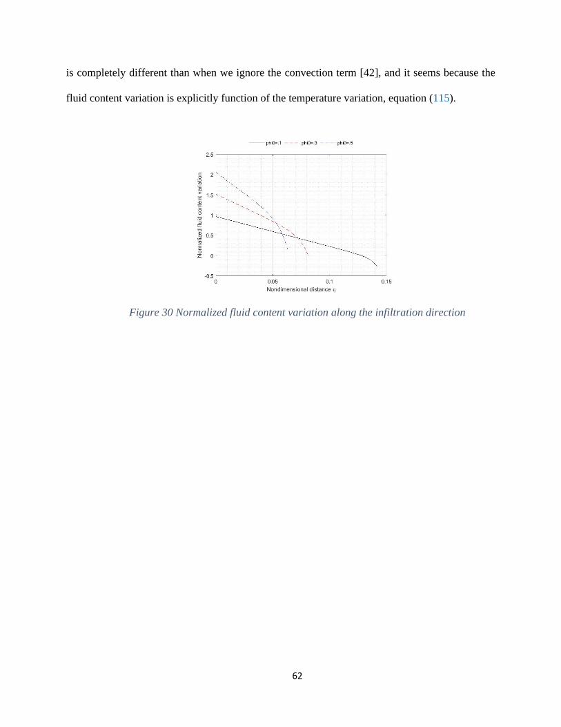
62

is completely different than when we ignore the convection term [42], and it seems because the

fluid content variation is explicitly function of the temperature variation, equation (115).

Figure 30 Normalized fluid content variation along the infiltration direction

63

5 CONCLUSION

This thesis presents self-similar analytical solutions for one-dimensional, linear and radial,

isothermal, non-Newtonian fluid flows in a porous solid with two types of boundary conditions; a

specified applied pressure and a specified inlet fluid flux factor. It also presents a self-similar

numerical solution of one-dimensional, linear, non-isothermal, Newtonian fluid flow in a porous

solid with specified applied pressure and temperature boundary conditions considering convection

heat transfer. The self-similar solutions are valid for infiltration of a long porous solid by the fluids.

The main conclusions for the isothermal infiltration of porous solid by a non-Newtonian

fluid, which can be withdrawn from the results of this thesis, are as follows:

1. The infiltration front is a function of time according to 𝑡𝑛

𝑛+1, where n is the flow behavior

index.

2. The infiltration front advances faster in the linear infiltration than in the radial infiltration.

3. Increasing the flow behavior index n for the non-Newtonian fluid increases the non-

dimensional infiltration front, while decreasing the solid porosity increases the dimensional

and non-dimensional infiltration front.

4. Regarding the pore pressure distribution, the results show that it is almost linear in the

linear infiltration, while it is non-linear in the radial infiltration and it drops to zero at the

infiltration front.

The main conclusions for the non-isothermal infiltration of porous solid by a Newtonian

fluid, which can be withdrawn from the results of this thesis, are as follows:

1. For non-isothermal 1D linear flow of a Newtonian fluid, the dimensional infiltration front

varies with time according to 𝑡1

2. The infiltration front increases with a decrease in the

porosity of the porous solid. The pore pressure varies almost linearly from the inlet to the

64

infiltration front, where it reaches zero. While, the temperature variation increases, when

the initial temperature variation is negative, along the infiltration direction and reaches zero

at a distance farther than the infiltration front, not at the infiltration front.

2. The infiltration front is a function of time according to 𝑡1

2.

3. The pore pressure is almost linear along the flow direction and reaches zero at the

infiltration front.

4. The fluid content variation is a function of the preform porosity in the non-isothermal linear

Newtonian infiltration.

5. The temperature variation increases, when the initial temperature variation at the inlet is

negative, non-linearly along the infiltration direction and reaches zero at a distance farther

than the infiltration front. Most of the heat transfer happens close to the infiltration front.

6. By comparing the results with that without considering convection [42], it appears that the

convection does not affect the infiltration front or the pore pressure. However, the

convection does affect the temperature variation and the fluid content variation, which is a

function of the temperature variation.

65

6 REFERENCES

[1] C Ikoku and H Ramey, “Transient Flow of Non-Newtonian Power-Law Fluids in Porous

Media,” Soc. Pet. Eng. J., vol. 19, no. 3, pp. 164–174, 1979.

[2] Y Wu, K Pruess, and P Witherspoon, “Flow and Displacement of Bingham Non-

Newtonian Fluids in Porous Media,” SPE Reserv. Eng., vol. 7, no. 3, pp. 369–376, 1992.

[3] A. M. Alsofi and Martin Blunt, “Streamline-Based Simulation of Non-Newtonian

Polymer Flooding,” SPE J., vol. 15, no. 4, pp. 895–905, 2010.

[4] M Endo Kokubun, F Radu, E Keilegavlen, K Kumar, and K Spildo, “Transport of

Polymer Particles in Oil–Water Flow in Porous Media: Enhancing Oil Recovery,”

Transp. Porous Media, vol. 126, no. 2, pp. 501–519, 2018.

[5] A Mortensen, V Michaud, and M Flemings, “Pressure-infiltration processing of

reinforced aluminum,” JOM, vol. 45, no. 1, pp. 36–43, 1993.

[6] Y.-S. WU, K. PRUESS, and P. A. WITHERSPOON, “Displacement of a Newtonian

Fluid by a Non-Newtonian Fluid in a Porous Medium,” Transp. Porous Media, vol. 6, no.

2, 1991.

[7] Karen S. Pedersen and Hans P. Ronningsen, “Effect of Precipitated Wax on Viscosity-A

Model for Predicting Non-Newtonian Viscosity of Crude Oils,” Energy & Fuels, vol. 14,

no. 1, pp. 43–51, 2000.

[8] G. I. Barenblatt, V. M. Entov, and V. M. Ryzhik, Theory of fluid flows through natural

rocks. Dordrecht: Kluwer, 1990.

[9] X Dong, H Liu, Q Wang, Z Pang, and C Wang, “Non-Newtonian flow characterization of

heavy crude oil in porous media,” J. Pet. Explor. Prod. Technol., vol. 3, no. 1, pp. 43–53,

2012.

[10] W Kozicki, A Rao, and C Tiu, “Filtration of polymer solutions,” Chem. Eng. Sci., vol.

27, no. 3, pp. 615–626, 1972.

66

[11] A. Uscilowska, “Non-Newtonian fluid flow in a porous medium,” J. Mech. Mater.

Struct., vol. 3, no. 6, 2008.

[12] T. Sochi, “Flow of Non-Newtonian Fluids in Porous Media,” Wiley Online Libr., vol. 48,

no. 23, pp. 2437–2467, 2010, doi: 10.1002/polb.22144.

[13] V. Di and F. Valentina, “Generalized Solution for 1-D Non-Newtonian Flow in a Porous

Domain due to an Instantaneous Mass Injection,” Transp. Porous Media, vol. 93, no. 1,

pp. 63–77, 2012, doi: 10.1007/s11242-012-9944-9.

[14] G. Lewis, “Viscoelastic properties of injectable bone cements for orthopaedic

applications: State-of-the-art review,” J. Biomed. Mater. Res. Part B Appl. Biomater.,

vol. 98B, no. 1, pp. 171–191, 2011.

[15] H Park, M Hawley, and R Blanks, “The flow of non-Newtonian solutions through packed

beds,” Polym. Eng. Sci., vol. 15, no. 11, pp. 761–773, 1975.

[16] R. P. Chhabra, J. Comiti, and I. Machac, “Flow of non-Newtonian fluids in fixed and

fluidised beds,” Chem. Eng. Sci., vol. 56, no. 1, pp. 1–27, 2001.

[17] J Wannasin and M Flemings, “Fabrication of metal matrix composites by a high-pressure

centrifugal infiltration process,” J. Mater. Process. Technol., vol. 169, no. 2, pp. 143–

149, 2005.

[18] S. G Fishman and A. K. Dhingra, Cast reinforced metal composites. ASM International,

1988.

[19] J. Warren H. Hunt, “Aluminum Metal Matrix Composites Today,” Mater. Sci. Forum,

vol. 331–337, pp. 71–84, 2000.

[20] V. Michaud and A. Mortensen, “Infiltration processing of fibre reinforced composites:

governing phenomena,” Compos. Part A Appl. Sci. Manuf., vol. 32, no. 8, pp. 981–996,

2001.

[21] D. Kopeliovich, Advances in Ceramic Matrix Composites. 2014.

67

[22] T. Ouahbi, A. Saouab, P. Ouagne, S. Chatel, and J. Bre, “Modelling of hydro-mechanical

coupling in infusion processes,” vol. 38, pp. 1646–1654, 2007, doi:

10.1016/j.compositesa.2007.03.002.

[23] A Coldea, M Swain, and N Thiel, “Mechanical properties of polymer-infiltrated-ceramic-

network materials,” Dent. Mater., vol. 29, no. 4, pp. 419–426, 2013.

[24] H. Pascal, “Rheological behaviour effect of non‐newtonian fluids on steady and unsteady

flow through a porous medium,” Int. J. Numer. Anal. Methods Geomech., vol. 7, no. 3,

pp. 289–303, 1983, doi: 10.1002/nag.1610070303.

[25] H. Pascal, “Rheological effects of non-Newtonian behavior of displacing fluids on

stability of a moving interface in radial oil displacement mechanism in porous media,”

Int. J. Eng. Sci., vol. 24, no. 9, pp. 1465–1476, 1986.

[26] H. Pascal, “Stability of non-newtonian fluid interfaces in a porous medium and its

applications in an oil displacement mechanism,” J. Colloid Interface Sci., vol. 123, no. 1,

pp. 14–23, 1988, doi: 10.1016/0021-9797(88)90216-0.

[27] H. Pascal, “Some Self-Similar Flows of Non-Newtonian Fluids through a Porous

Medium,” Stud. Appl. Math., vol. 82, no. 1, pp. 1–12, 1990, doi: 10.1002/sapm19908211.

[28] H. Pascal, “Dynamics of moving interface in porous media for power law fluids with

yield stress,” Int. J. Eng. Sci., vol. 22, no. 5, pp. 577–590, 1984.

[29] H. Pascal, “On non-linear effects in unsteady flows of non-newtonian fluids through

fractured porous media,” Int. J. Non. Linear. Mech., vol. 26, no. 5, pp. 487–499, 1991.

[30] H. Pascal and F. Pascal, “Flow of non-newtonian fluid through porous media,” Int. J.

Eng. Sci., vol. 23, no. 5, pp. 571–585, 1985.

[31] S.E. Buckley and M.C. Leverett, “Mechanism of Fluid Displacement in Sands,” Trans.

AIME, vol. 146, no. 1, pp. 107–116, 1942.

[32] H. J. Welge, “A Simplified Method for Computing Oil Recovery by Gas or Water

Drive,” J. Pet. Technol., vol. 4, no. 04, pp. 91–98, 1952.

68

[33] Zhongxiang Chen and Ciqun Liu, “Self-similar solutions for displacement of non-

Newtonian fluids through porous media,” Transp. Porous Media, vol. 6, no. 1, pp. 13–33,

1991.

[34] V Di Federico, M Pinelli, and R Ugarelli, “Estimates of effective permeability for non-

Newtonian fluid flow in randomly heterogeneous porous media,” Stoch. Environ. Res.

Risk Assess., vol. 24, no. 7, pp. 1067–1076, 2010.

[35] R.H. Christopher and S. Middleman, “Power-Law Flow through a Packed Tube,” Ind.

Eng. Chem. Fundam., vol. 4, no. 4, pp. 422–426, 1965.

[36] W. KOZICKI, C. J. Hsu, and C. TIU, “Non-Newtonian flow through packed beds and

porous media,” Chem. Eng. Sci., vol. 22, no. 4, pp. 487–502, 1967.

[37] J.R.A. Pearson and P.M.J. Tardy, “Models for flow of non-Newtonian and complex

fluids through porous media,” J. Nonnewton. Fluid Mech., vol. 102, no. 2, pp. 447–473,

2002.

[38] V. Ciriello and V. Di Federico, “Analysis of a benchmark solution for non-Newtonian

radial displacement in porous media,” Int. J. Non. Linear. Mech., vol. 52, pp. 46–57,

2013, doi: 10.1016/j.ijnonlinmec.2013.01.011.

[39] E. Lacoste, O. Mantaux, and M. Danis, “Numerical simulation of metal matrix

composites and polymer matrix composites processing by infiltration : a review,”

Compos. Part A Appl. Sci. Manuf., vol. 33, no. 12, pp. 1605–1614, 2002.

[40] C Jung, J Jang, and K Han, “Numerical Simulation of Infiltration and Solidification

Processes for Squeeze Cast Al Composites with Parametric Study,” Metall. Mater. Trans.

A, vol. 39, no. 11, pp. 2736–2748, 2008.

[41] H. Prielipp et al., “Strength and fracture toughness of aluminum / alumina composites

with interpenetrating networks,” Mater. Sci. Eng. A, vol. 197, no. 1, pp. 19–30, 1995.

[42] Z. Jin, “A thermo-poroelasticity theory for infiltration processing of interpenetrating

phase composites,” Acta Mech., vol. 229, no. 10, pp. 3993–4004, 2018, doi:

10.1007/s00707-018-2202-7.

69

[43] M. P. Walsh and L. W. Lake, “APPLYING FRACTIONAL FLOW THEORY TO

SOLVENT FLOODING AND CHASE FLUIDS,” J. Pet. Sci. Eng., vol. 2, no. 4, pp.

281–303, 1989.

[44] G. A. Pope, “The Application of Fractional Flow Theory to Enhanced Oil Recovery,”

Soc. Pet. Eng. J., vol. 20, no. 3, pp. 191–205, 1980.

[45] W. R. Rossen and et al., “Fractional Flow Theory Applicable to Non-Newtonian

Behavior in EOR Processes,” Transp. Porous Media, vol. 89, no. 2, pp. 213–236, 2011,

doi: 10.1007/s11242-011-9765-2.

[46] D. Ambrosi, “Infiltration through Deformable Porous Media,” ZAMM, vol. 82, no. 2, pp.

115–124, 2002.

[47] R. Larsson, M. Rouhi, and M. Wysocki, “European Journal of Mechanics A / Solids Free

surface fl ow and preform deformation in composites manufacturing based on porous

media theory,” Eur. J. Mech. / A Solids, vol. 31, no. 1, pp. 1–12, 2012, doi:

10.1016/j.euromechsol.2011.06.015.

[48] P. C. Dawson, “Flow Properties of Molten Polymers,” Polym. Sci. Technol. Ser., pp. 88–

95, 1999.

[49] G. M. Swallowe, Mechanical properties and testing of polymers. Dordrecht: Kluwer,

2010.

[50] G. H. R. Kefayati, “Simulation of non-Newtonian molten polymer on natural convection

in a sinusoidal heated cavity using FDLBM,” J. Mol. Liq., vol. 195, pp. 165–174, 2014,

doi: 10.1016/j.molliq.2014.02.031.

[51] E. Detournay and A. H. D. Cheng, “Fundamentals of poroelasticity,” Compr. rock Eng.

Vol. 2, vol. II, pp. 113–171, 1993, doi: 10.1016/b978-0-08-040615-2.50011-3.

[52] M. Kurashige, “A thermoelastic theory of fluid-filled porous materials,” Int. J. Solids

Struct., vol. 25, no. 9, pp. 1039–1052, 1989, doi: 10.1016/0020-7683(89)90020-6.

70

[53] N. Noda, R. B. Hetnarski, and Y. Tanigawa, Thermal Stresses, 2nd edn. New York:

Taylor & Francis, 2003.

[54] Z. H. Jin, K. Tohgo, T. Fujii, and Y. Shimamura, “Double edge thermal crack problem

for an interpenetrating phase composite: Application of a matricity-based thermal

conductivity model,” Eng. Fract. Mech., vol. 177, pp. 167–179, 2017, doi:

10.1016/j.engfracmech.2017.03.034.

[55] Z. Hashin and S. Shtrikman, “A Variational approach to the theory of the effective

magnetic permeability of multiphase materials,” J. Appl. Phys., vol. 33, no. 10, pp. 3125–

3131, 1962, doi: 10.1063/1.1728579.

[56] [1]V. Michaud, A. Mortensen and J. Sommer, "Infiltration of fibrous preforms by a pure

metal: Part V. Influence of preform compressibility", Metallurgical and Materials

Transactions A, vol. 30, no. 2, pp. 471-482, 1999. Available: 10.1007/s11661-999-0337-

9.

[57] Vlachopoulos, John, and Nickolas Polychronopoulos. “Basic Concepts in Polymer Melt

Rheology and Their Importance in Processing.” Applied Polymer Rheology: Polymeric

Fluids with Industrial Applications, no. January 2012, 2011, pp. 1–27,

doi:10.1002/9781118140611.ch1.

71

7 BIOGRAPHY OF THE AUTHOR

Hamza Azzam was born in San Luis Obispo, California on June 22, 1994. He was raised

in Egypt and graduated from Mit-Rahina High School in 2012. He attended Cairo University and

graduated in 2017 with a Bachelor’s degree in Mechanical Power Engineering. He started the

Mechanical Engineering graduate program at the University of Maine in the Fall of 2018. After

receiving his Master’s degree, he will continue graduate school at the University of Maine to

pursue a Ph.D. degree in Mechanical Engineering. Hamza is a candidate for the Master of Science

degree in Mechanical Engineering from the University of Maine in December 2020.

Modeling of Non-Newtonian Fluid Flow in a Porous Medium

Documents

Transcript of Modeling of Non-Newtonian Fluid Flow in a Porous Medium