MODELING OF MULTI-STAGE FRACTURED HORIZONTAL WELLS...
191
MODELING OF MULTI-STAGE FRACTURED HORIZONTAL WELLS A Thesis Submitted to the Faculty of Graduate Studies and Research in Partial Fulfillment of the Requirements for the Degree of Master of Applied Science in Petroleum Systems Engineering University of Regina By Shanshan Yao Regina, Saskatchewan December 2013 Copyright 2013: Shanshan Yao
Transcript of MODELING OF MULTI-STAGE FRACTURED HORIZONTAL WELLS...
MODELING OF MULTI-STAGE FRACTURED
HORIZONTAL WELLS
A Thesis
Submitted to the Faculty of Graduate Studies and Research
in Partial Fulfillment of the Requirements
for the Degree of
Master of Applied Science
in Petroleum Systems Engineering
University of Regina
By
Shanshan Yao
Regina, Saskatchewan
December 2013
Copyright 2013: Shanshan Yao

UNIVERSITY OF REGINA
FACULTY OF GRADUATE STUDIES AND RESEARCH
SUPERVISORY AND EXAMINING COMMITTEE
Shanshan Yao, candidate for the degree of Master of Applied Science in Petroleum Systems Engineering, has presented a thesis titled, Modeling of Multi-Stage Fractured Horizontal Wells, in an oral examination held on November 22, 2013. The following committee members have found the thesis acceptable in form and content, and that the candidate demonstrated satisfactory knowledge of the subject material. External Examiner: Dr. Tsun Wai Kelvin Ng, Environmental Systems Engineering
Co-Supervisor: Dr. Fanhua Zeng, Petroleum Systems Engineering
Co-Supervisor: Dr. Gang Zhao, Petroleum Systems Engineering
Committee Member: Dr. Farshid Torabi, Petroleum Systems Engineering
Committee Member: Dr. Exeddin Shirif, Petroleum Systems Engineering
Chair of Defense: Dr. Chun-Hua Guo, Department of Mathematics & Statistics
I
ABSTRACT
Horizontal wells stimulated by multiple fractures unlock tight formations and
shale gas reservoirs that used to be considered as uneconomic plays. However,
the popularity of such techniques presents new challenges to the reservoir and
fractures evaluation. Fractured horizontal wells’ pressure and production rate
behaviour exhibit complex trends that are quite different from previous horizontal
and fractured vertical wells. To facilitate the pressure and rate analysis, this
work developed semi-analytical models under different assumptions and
comprehensively described the fluid flow of a multi-stage fractured horizontal
well in a bounded reservoir.
The governing Partial Differential Equations (PDEs) in this work are highly
nonlinear, and, therefore, analytical methods are not applicable to obtaining
results of drawdown and build-up tests. The semi-analytical modeling method
here shows advantages in applicability over the analytical modeling.
For fractured horizontal wells with constant fracture conductivities, four
kinds of fluid flow, including flow from the reservoir to fractures and to the
horizontal wellbore, flow inside the fractures as well as inside the horizontal
wellbore were all taken into consideration. Standard type curves for transient
pressure analysis were documented. The unique pressure behaviour reveals
that multiple fractures play a more important role than the horizontal wellbore in
the whole system. Also, the applicability of these type curves in the transient
II
pressure analysis was proved when compared with the method based on typical
characteristic lines.
The stress-sensitive hydraulic fracture conductivity was the other factor
incorporated into the semi-analytical models. A series of type curves were also
generated to evaluate the fractures’ stress-dependent characteristics. Stress-
dependent conductivities can cause pressure and pressure derivative curves to
increase rapidly, which seem to be “apparent boundary-dominated flow”. The
influence of these changing conductivities strongly depends on the fractures’
properties (i.e., fracture stress-sensitive characteristic value df and initial fracture
conductivity CfDi.).
When the bottomhole flowing pressure remains constant, the semi-
analytical model can be further used to study the fractured horizontal wells’
production rate behaviour. After the comparison with analytical solutions, it can
be concluded that horizontal wells with multi-stage fractures produce as if the
fractures worked individually at early times. Moreover, if considering the stress-
sensitive fracture conductivities, the straight lines of reciprocal rates vs. time
exhibit special slopes deviate from 1/4 and 1/2 for bilinear and linear flow,
respectively.
In addition to the advantages over analytical methods, the methodology and
models presented are flexible and widely applicable as numerical models.
Remarkable progress can be achieved if the methodology is extended to solve
flow problems in complex fracture systems and dynamic matrix permeability.

III
ACKNOWLEDGEMENTS
I would like to take this opportunity to express my sincere appreciation and
gratitude to my co-supervisors, Dr. Fanhua Zeng and Dr. Gang Zhao, for their
guidance and support throughout my studies. Their encouragement, expertise,
advice, and enthusiasm helped me accomplish this study.
I also would like to thank my family: Jianhua Yao and Xianxia Zeng (my
parents) and Yulong Yao (my brother) for their endless love and understanding
during my graduate studies.
Acknowledgment is due to the Faculty of Graduate Studies and Research at
the University of Regina for financial support in the form of scholarships.
Furthermore, I am thankful to the members of my examination committee and
their valuable suggestions in this study. I also thank Heidi Smithson for her
proofreading.
I would also like to thank my colleagues, Ms. Lijuan Zhu, Ms. Suxin Xu, Mr.
Tao Jiang, Mr. Xinfeng Jia, and Mr. Zuojing Zhu for their care and helpful
discussion regarding this work.

IV
DEDICATION
To
My best friend and companion, Mr. Ning Ju,
and my loving parents Mr. Jianhua Yao and Ms. Xianxia Zeng.
V
TABLE OF CONTENTS
ABSTRACT ······················································································ I
ACKNOWLEDGEMENTS ······································································ III
DEDICATION ···················································································· IV
TABLE OF CONTENTS ·········································································V
LIST OF TABLES ················································································ IX
LIST OF FIGURES ················································································X
LIST OF APPENDICES ······································································ XIV
NOMENCLATURE ··············································································XV
CHAPTER 1 INTRODUCTION ······························································ 1
1.1 Multi-stage hydraulic fracturing ························································ 1
1.2 Scope and objectives of this study ···················································· 4
1.3 Organization of this dissertation ······················································· 5
CHAPTER 2 LITERATURE REVIEW ····················································· 7
2.1 Modeling multi-stage fractured horizontal wells ··································· 8
2.1.1 Analytical modeling ·········································································· 8
2.1.2 Numerical modeling ······································································· 10
2.1.3 Summary ····················································································· 11
2.2 Modeling horizontal wells with stress-sensitive hydraulic fractures ········ 11
2.2.1 Laboratory observations of stress-sensitive hydraulic fractures ················ 11
2.2.2 Modeling stress-sensitive hydraulic fractures ······································· 12
2.2.3 Fluid flow modeling with stress-sensitive hydraulic fractures ···················· 13
VI
2.2.4 Summary ····················································································· 15
2.3 Multi-stage fractured horizontal well production rate analysis ··············· 16
2.3.1 Decline curve analysis ···································································· 16
2.3.2 Type curve analysis ······································································· 18
2.3.3 Summary ····················································································· 20
2.4 Chapter Summary ······································································· 21
CHAPTER 3 METHODOLOGY ··························································· 23
3.1 Green’s functions and source/sink solutions ····································· 23
3.1.1 Green’s and source/sink function ······················································ 23
3.1.2 Newman product ··········································································· 25
3.2 Laplace transformation ································································· 26
3.3 Continuity conditions ···································································· 26
3.4 Constructing and solving linear equation systems ······························ 28
3.5 Chapter summary ········································································ 29
CHAPTER 4 MULTI-STAGE HYDRAULICALLY FRACTURED
HORIZONTAL WELLS ··················································· 30
4.1 Model and algorithm ···································································· 30
4.1.1 Dimensionless variables ·································································· 32
4.1.2 Mathematical model ······································································· 34
4.1.3 Algorithm ····················································································· 37
4.2 Model validation ·········································································· 43
4.3 Results and discussion ································································· 46
4.3.1 Effect of fluid flow from reservoir to horizontal wellbore··························· 46
4.3.2 Effect of horizontal wellbore pressure drop ·········································· 49

VII
4.3.3 Effect of fracture stages ·································································· 51
4.3.4 Effect of gas desorption ·································································· 61
4.3.5 Effect of skin factors ······································································· 64
4.4 Field examples ··········································································· 68
4.4.1 No.1 Build-up test analysis ······························································ 68
4.4.1 No.2 Build-Up test analysis ······························································ 69
4.5 Chapter summary ········································································ 75
CHAPTER 5 HYDRAULICALLY FRACTURED WELLS WITH STRESS-
SENSITIVE CONDUCTIVITIES ········································· 77
5.1 Model and algorithm ···································································· 78
5.2 Model validation ·········································································· 82
5.3 Results and discussion ································································· 85
5.3.1 Pressure behaviour characteristics ··················································· 85
5.3.2 Effect of degree of stress-sensitivity ··················································· 92
5.3.3 Effect of degree of conductivity loss ··················································· 96
5.3.4 Effect of initial conductivity ····························································· 100
5.3.5 Stress-sensitive conductivity ·························································· 102
5.4 Field example ··········································································· 105
5.4.1 Analysis without corrections in matrix permeability ······························ 105
5.4.2 Analysis with corrections in matrix permeability only ···························· 110
5.5 Chapter summary ······································································ 116
VIII
CHAPTER 6 PRODUCTION RATE ANALYSIS ··································· 118
6.1 Model and algorithm ·································································· 119
6.2 Model validation ········································································ 120
6.3 Results and discussion ······························································· 122
6.3.1 Comparison with analytical solutions of single-fractured wells ················ 122
6.3.2 Effect of stress-sensitive fracture conductivity ···································· 135
6.4 Field examples ········································································· 142
6.4.1 Marcellus shale gas well A ····························································· 142
6.4.2 Marcellus shale gas well B ····························································· 147
6.5 Chapter summary ······································································ 152
CHAPTER 7 Conclusions and Recommendations ····························· 153
7.1 Conclusions ············································································· 153
7.2 Recommendations ···································································· 155
List of References ··········································································· 156
APPENDIX A SOURCE FUNCTIONS ················································· 167
APPENDIX B SOLUTIONS OF FLUID FLOW INSIDE HYDRAULIC
FRACTURES ······························································ 170

IX
LIST OF TABLES
Table 4.1 Basic input parameters. ··················································· 71
Table 5.1 Reservoir, well, fracture and fluid data. ······························· 88
Table 5.2 Results of field case analysis. ········································· 114

X
LIST OF FIGURES
Figure 1.1 Schematic of a multi-stage fractured horizontal well. ················ 3
Figure 4.1 A multi-stage fractured horizontal well in a box-shaped reservoir.
···················································································· 31
Figure 4.2 Diagram showing fracture and horizontal wellbore discretization.
···················································································· 39
Figure 4.3 Flow chart for modeling and solving process. ······················ 44
Figure 4.4 Model validation with Kappa Ecrin. ····································· 45
Figure 4.5 Effect of fluid flow from reservoir to the wellbore. ··················· 47
Figure 4.6 Flow distribution along the fracture and wellbore. ·················· 48
Figure 4.7 Effect of horizontal wellbore pressure drop. ·························· 50
Figure 4.8 Effect of fracture stages when xf is constant. ························ 55
Figure 4.9 Effect of fracture stages on the productivity index with costant
xf. ················································································· 56
Figure 4.10 Effect of fracture stages when fracture volume is constant. ····· 57
Figure 4.11 Effect of fracture stages on the productivity indxex with cosntant
Vf. ················································································ 58
Figure 4.12 Non-uniform fractures along the horizotnal wellbore. ·············· 59
Figure 4.13 Effect of non-uniform fractures on the pressure behaviour . ····· 60
Figure 4.14 Effect of gas desorption on pressure behaviour . ··················· 63
Figure 4.15 Effect of skin factors on the pressure behaviour . ·················· 66
Figure 4.16 Effect of skin factors on the flow distribution along the fracture. 67
XI
Figure 4.17 Field production data. ······················································ 70
Figure 4.18 Plot of adjusted pressure vs. fourth root time. ······················· 72
Figure 4.19 Type curve match for the first test. ····································· 73
Figure 4.20 Type curve match for the second test.································· 74
Figure 5.1 Discretizing the fracture system. ········································ 80
Figure 5.2 Discretizing the fracture conductivity. ·································· 80
Figure 5.3 Model validation. ···························································· 84
Figure 5.4 Transient pressure behaviour with stress-sensitive hydraulic
fractures. ······································································· 89
Figure 5.5 Modified smooth conductivity curve. ···································· 90
Figure 5.6 Pressure behavior based on modified conductivity change. ····· 91
Figure 5.7 Normalized fractures conductivities change with stress (Abass et
al., 2009 and Zhang, et al., 2013) ······································· 94
Figure 5.8 Type curves showing the effect of stress-sensitive conductivity,
CfDi=50, CfDmin=0.25. ························································ 95
Figure 5.9 Normalized fracture conductivity (Abass et al., 2009) ············· 98
Figure 5.10 Type curves showing the effect of minimum conductivity, CfDi=50
and df=1×10⁻⁷Pa-1. ··························································· 99
Figure 5.11 Type curves showing the effect of initial conductivity,
CfDi/CfDmin=200. ······························································ 101
Figure 5.12 Variation of fracture conductivity ratio with different df and CfDi.104
XII
Figure 5.13 Gas and water production rates, and calculated flowing
bottomhole pressures (Clarkson et al., 2012). ··················· 107
Figure 5.14 Pressure and pressure derivative without corrections in
matrix permeability (Clarkson et al., 2012). ························ 108
Figure 5.15 Type curve matching results without corrections in
matrix permeability. ······················································ 109
Figure 5.16 Pressure and pressure derivative with corrections in
matrix permeability (Clarkson et al., 2012). ························ 112
Figure 5.17 Type curve matching results with corrections in matrix
permeability. ······························································· 113
Figure 5.18 Production rate prediction. ············································· 115
Figure 6.1 Model validation. ·························································· 121
Figure 6.2 Results comparison for bilinear flow. ································ 124
Figure 6.3 Results comparison for linear flow. ·································· 127
Figure 6.4 Production rates with different fracture half-lengths. ············ 130
Figure 6.5 Results comparison for compound linear flow. ··················· 131
Figure 6.6 Results comparison for boundary-dominated flow. ·············· 134
Figure 6.7 Production curves with different df. ·································· 137
Figure 6.8 Conductivity curves with different df.·································································· 138
Figure 6.9 Production curves with different initial conductivity CfDi. ······· 140
Figure 6.10 Conductivity curves with different CfDi. ······························ 141
Figure 6.11 Plot of reciprocal gas rate vs. fourth root of time. ················ 143
Figure 6.12 Plot of reciprocal gas rate vs. square root of time. ·············· 144
XIII
Figure 6.13 Type curve matching for Marcellus shale gas well A. ·········· 146
Figure 6.14 Diagnostic plot of production rate vs. time. ························ 149
Figure 6.15 Plot of reciprocal gas rate vs. square root of time. ·············· 149
Figure 6.16 Type curves based on parameters from analytical
solutions. ···································································· 150
Figure 6.17 Type curve matching result by semi-analytical model. ········· 151

XIV
LIST OF APPENDICES
APPENDIX A Source functions ························································· 167
APPENDIX B Solutions of fluid flow inside hydraulic fractures ················· 170
XV
NOMENCLATURE
a = reservoir length, L, m
b = reservoir width, L, m
ct =total compressibility, L2/m, pa-1
tc =total compressibility at pressure in the region of influence, L2/m, pa-1
cg = gas compressibility, L2/m, pa-1
C =gas concentration at the surface of pore walls, n/L3, mole/ m3
Cw =wellbore storage, L5/m, m3/Pa
Cf = fracture conductivity, L3, m3
Cη = fracture diffusivity, dimensionless
df = fracture stress-dependent characteristic, L2/m, Pa-1
h = net-pay thickness, L, m
J=pseudo-steady state productivity index, L5/(t∙m), m3/(Pa∙s)
k = reference permeability, L2, m2
k =permeability at pressure in the region of influence, L2, m2
ks = fracture-face skin zone permeability, L2, m2
NRe= Reynolds number, dimensionless
NRe,w = Inflow Reynolds number, dimensionless
p = pressure, m/L2, Pa
pa=adjusted pressure, m/L2, Pa
q = flow rate, L3/t, m3/s
qf = flow rate normal to fracture, L2/t, m2/s
XVI
qh = flow rate normal to horizontal wellbore, L2/t, m2/s
Q=reference flow rate, L3/t, m3/s
RD=dimensionless desorption storability ratio
sck = choked-fracture-skin factor, dimensionless
sff = fracture-face skin factor, dimensionless
S= strength of source, dimensionless
t = time, t, s [hr]
T =temperature, T, K
u=Laplace variable
v = velocity, L3/s, m3/s
wf = fracture width, L, m
xck = choke length in one fracture wing, L, m
xf =fracture half-length, L, m
z = deviation factor, dimensionless
μ = viscosity, m/(L2∙t), Pa∙s
=viscosity evaluated at pressure in the region of influence, m/L, Pa∙s
ρ = density, m/L3, g/cm3
ϕ= porosity, fraction
Ω= segment number
Γ=segment interface
τ=time variable in integration, t, s
Subscripts
D = dimensionless

XVII
f = fracture
h= horizontal well
i=initial condition.
min=minimum value.
r = reference length
wf= wellbore bottomhole condition
sc= standard conditions

1
CHAPTER 1
INTRODUCTION
1.1 Multi-stage hydraulic fracturing
Hydraulic fracturing is a technique during which typically a mixture of water,
propping agents (usually sands), and chemicals is pumped at sufficiently high
rates and pressure into the pay zone to create fractures (Ralph,1983). Created
fractures can provide conduits for gas, oil, and water to easily migrate towards
the well. The fracture usually has two wings extending in opposite directions
from the well.
The first hydraulic fracturing experiment was conducted in 1947 at the
Hugoton gas field, Grant Country, Kansas, USA (Clark, 1949). In 1949, two
commercial hydraulic fracturing treatments were introduced into the industry in
Oklahoma and Texas. Since then, the hydraulic fracturing technique has
evolved into a standard operating practice and approximately 2.5 million of such
treatments have been performed globally.
As target formations became deeper, hotter, and lower in permeability,
massive hydraulic fracturing (MHF) emerged in 1968 to address the associated
challenges. The definition of MHF varies but generally refers to the treatments
injecting up to 3.8×10³ m3 (1×10⁶ gal) fracturing fluid and more than 1.36×10⁶ Kg
(3×10⁶ lbm) propping agent (Ben and Spencer, 1993). MHF treatments
significantly improve wells’ productivity by creating large and high-conductivity
fractures, especially in tight and shale formations.
2
Horizontal well completion is another technique that has proved to be much
more effective than vertical wells for tight chalk and shale formations. The
horizontal wellbore extends horizontally within the target formation to a
predetermined bottomhole location. This lateral wellbore makes it easier to
conduct multiple fracturing treatments for one well.
In the late 1980s, operators in Texas began to combine horizontal drilling
with MHF treatments. The hydraulic fracturing technique evolved from single-
stage operation to multi-stage (40 plus) fracturing. Multi-stage fracturing begins
at the toe of the long horizontal wellbore and extends down to the heel. For each
stage, the corresponding wellbore section is isolated, and then, water is pumped
to crack the formation. Sand carried along with the water can prop the facture.
Figure 1.1 shows the schematic of a multi-stage fractured horizontal well.
Multi-stage fractured horizontal wells are crucial to unconventional reservoir
development. Prior to the popularity of multi-stage fractured horizontal wells,
unconventional resources were always overlooked by operators. Take the
Barnett Shale as an example. Before 1980, Barnett Shale was known to have
essentially zero permeability and, thus, was considered uneconomic. However,
the gas production from multi-stage fractured horizontal wells in Barnett Shale
increased to about 5 Bcf per day in 2010 with application of multi-stage fractured
horizontal wells .( United States Department of Energy, 2011).

3
(Original in color)
Figure 1.1― Schematic of a multi-stage fractured horizontal well (Mitch, 2010).
4
Several mechanisms have been proposed to explain the advantages of
multi-stage hydraulic fracturing over other techniques. At first, multiple hydraulic
fractures provide more “superhighways” than single-stage fractured vertical
wells. Moreover, the increasing stages can substantially enlarge the contacted
reservoir area. Furthermore, there always exist open natural fractures in tight
and shale formations. The interaction between hydraulic fractures and the
natural-fracture network expands the stimulated reservoir volume (SRV) beyond
which the remaining reservoir is usually negligible (Medeiros et al. 2008;
Mayerhofer et al. 2010).
Although multi-stage fractured horizontal wells are efficient, analyzing and
predicting such wells’ performance are challenging not only because of
potentially complex reservoir behaviour (dual porosity/dual permeability, multi-
layer, stress-dependent porosity and permeability, multi-phase flow, etc.), but
also because of the complex sequence of flow regimes that evolve over time
during production (Clarkson and Pedersen, 2010). Hence, advanced production
analysis methods are highly appreciated.
1.2 Scope and objectives of this study
The objectives of this study are to develop a set of semi-analytical
methodologies to rigorously model the fluid flow behaviour in reservoirs with
multi-stage fractured horizontal wells, to present standard type curves for
identifying matrix and fracture properties with transient pressure and production
rate data, and to help petroleum engineers better understand the fractured
horizontal wells’ influence on reservoir development.
5
This work focuses on single-phase slightly compressible fluid flow in porous
media. The multi-stage fractured horizontal well exists in a whole homogeneous
reservoir. Hydraulic fracture conductivities could be constant or change along
with pressure. All above phenomena are rigorously modeled.
The influence of different parameters, including fracture half-lengths,
fracture conductivities, fracture stages, and the horizontal wellbore contribution,
on pressure and production rate behaviour is studied based on sensitivity
analysis. These results can be further applied in optimizing hydraulic fracturing
treatments. This study also derives analytical solutions that can be used to
evaluate and predict the production rates.
This study provides a general approach to accurately model complex fluid
flow in the reservoir with multi-stage fractured horizontal wells. This approach
can be further coupled with geomechanical methods in modeling the fracture-
formation interaction and rigorous PVT behaviour variation in transient pressure
and/or production rate analysis.
1.3 Organization of this dissertation
This dissertation is presented in seven chapters. Chapter 1 introduces the
background of multi-stage fractured horizontal wells. The objectives and
possible applications of this work are outlined. A comprehensive literature
review of scientific research on modeling multi-stage fractured horizontal wells is
conducted and limitations of current research are discussed in Chapter 2.
Chapter 3 presents the general methodology used in developing semi-analytical
models in this work. Chapter 4 shows a semi-analytical model and analyzes the

6
transient pressure behaviour of a multi-staged fractured horizontal well with
constant fracture conductivities. Type curves are shown with different
combinations of parameters. One field case is also analyzed. The effect of
stress-dependent hydraulic fracture conductivities on the transient pressure
behaviour is studied in Chapter 5. Another field example is introduced in this
chapter. In Chapter 6, the transient production rate behaviour of the fractured
horizontal well is analyzed based on my semi-analytical models and two field
examples. Several analytical solutions are also derived and tested in field
applications. Finally, Chapter 7 draws conclusions and provides
recommendations.
7
CHAPTER 2
LITERATURE REVIEW
Although multi-stage hydraulic fracturing is important for many
unconventional reservoirs, it is difficult to evaluate the fractures’ properties and
predict the wells’ performance since the transient pressure and production rate
behaviours are influenced by many factors, such as the reservoir permeabilities
and fracture conductivities. Therefore, accurately modeling and measuring the
effect of each parameter is necessary for better understanding the fractured
well/reservoir system.
Great effort and attempts have been made to model fractured wells during
recent decades. Related research in the literature and the related methodologies
used to model fractured wells are reviewed in this chapter. Based on the
objectives of this study, all these efforts and attempts in the literature can be
classified into the following three main categories:
Modeling multi-stage fractured horizontal wells with constant
properties,
Modeling hydraulically fractured wells with stress-sensitive
conductivities.
Modeling the production behaviour of fractured horizontal wells,
The literature review is also presented under the same categories as above.
8
2.1 Modeling multi-stage fractured horizontal wells
2.1.1 Analytical modeling
Although the Green’s function method had long been known, it was not
widely used in modeling flow behaviour in reservoirs until 1973. In 1973,
Gringarten and Ramey used the Green’s and source functions with the Newman
product method to generate reservoir transient-flow problem solutions. Pressure
response integration to an instantaneous source was applied to describe the
pressure behaviour of a continuous plane/slab source.
Gringarten et al. (1974) applied the source functions to model the pressure
behaviour of a well with a single infinite-conductivity vertical fracture. Compared
with Russell and Truitt’s work (1964), this new model is specifically useful in the
analysis of short-time field data. The analysis based on this model can provide
information concerning permeabilities, fracture lengths, and distance to a
symmetrical drainage limit.
The assumption of infinite conductivity is inapplicable for long and/or low-
conductive fractures. Then, Cinco-Ley and Samaniego (1981) developed a
mathematical model for the finite-conductivity fracture and used Laplace
transformation to solve the corresponding PDEs. Bilinear flow, which had never
been considered before, appears in the generated type curves.
Horizontal well drilling is another important technique in developing
reservoirs. In 1989, Babu and Odeh integrated point source functions and used
the simplified equations to describe the pressure behaviour of a horizontal well
9
in bounded reservoirs. However, the horizontal well must be parallel to one of
the boundaries.
Originally, horizontal wells were thought to have infinite conductivity, which
may lead to erroneous evaluation. In 1999, Penmatcha and Aziz proposed a
transient reservoir/wellbore coupling model for finite-conductivity horizontal wells
based on Babu and Odeh’s solutions. It was concluded that ignoring the
wellbore pressure drop could overpredict horizontal wells’ productivity.
All the above analytical solutions for fractured vertical wells and horizontal
wells laid a strong foundation for modeling multi-stage fractured horizontal wells
analytically.
In 1994, Guo and Evans developed a systematic methodology for modeling
a horizontal well intersecting multiple random discrete fractures, but the
interference between fractures was ignored, the study of which was undertaken
by Horne and Temeng (1995) who used the superposition principle on the basis
of Babu and Odeh’s solutions. In 1997, Chen and Raghavan rewrote Horne and
Temeng’s solutions by Laplace transformation according to Ozkan and
Raghavan who documented an extensive library of transient pressure solutions
for a wide variety of wellbore configurations in 1991.
One disadvantage of the source/sink function method is its inherent
singularity where the point source/sink is placed. In order to avoid this limitation,
Valkó and Amini (2007) developed the distributed volumetric sources (DVS)
method, which can also model the transient pressure behaviour.
10
In 2009, Ozkan, Raghavan, and Kazemi further presented an analytical tri-
linear flow model for fractured horizontal wells intercepted with natural fractures.
The dual-porosity inner reservoir between hydraulic fractures in this model is
naturally fractured. Mayerhofer et al. (2010) classified the stimulated reservoir
volume (SRV) in the fractured horizontal well system and suggested that
modeling SRV is important for evaluating the stimulation performance since the
contribution beyond the SRV can be ignored.
2.1.2 Numerical modeling
In numerical modeling of fractured horizontal wells, much effort has been
dedicated to representing fractures accurately and effectively.
In 1996, Herge studied the numerical simulation of fractured horizontal wells
in detail. He indicated that numerical models of fractured horizontal wells should
be dependent on the study objectives. If the early-time transient pressure
behaviour is required, explicit modeling of fractures and small grids near
fractures is appropriate. If the fractures are assumed to be infinite-conductive, it
is recommended to simply connect the wellbore to fractures and specify
connection factors.
In shale gas reservoirs, complex fractures networks are always generated
during multi-stage hydraulic fracture treatments. In 2009, Cipolla et al. proposed
the “LS-LR-DK” model to simulate fractured horizontal wells. In this model, the
single-plane propped fracture is modeled using a locally refined grid. Moreover,
the dual-permeability method is applied to represent fractures in both the
stimulated and unstimulated volumes. At last, grids in the stimulated volume are

11
further locally refined logarithmically. Also, the gas desorption effect and stress-
dependent fracture emerges in the model.
2.1.3 Summary
Both analytical solutions and numerical modeling are widely used for
fractured wells. Compared with analytical models, numerical solutions are
numerically unstable and time-consuming with excessively fine grid blocks.
Although accurate, analytical solutions are still limited to a series of assumption
and simplification. For example, in most cases, only one fracture is selected
from the whole system for detailed study under the assumption that all fractures
are the same. Therefore, a comprehensive semi-analytical model is required for
the multi-stage fractured horizontal wells, which incorporates analytical source
solutions and numerical discretization. Some phenomena that are visible in
unconventional reservoirs should also be added into this new mathematical
model.
2.2 Modeling horizontal wells with stress-sensitive hydraulic
fractures
2.2.1 Laboratory observations of stress-sensitive hydraulic fractures
Friedel et al. (2007) suggested the dependency of propped hydraulic
fracture permeabilities on reservoir pressure according to the experimental data
from Core Lab. Abass et al. (2009) and Zhang et al. (2013) also performed
experiments to investigate the propped fracture permeability vs. stress. Their
12
results indicate that the fracture conductivity can be reduced to a few to
hundreds of times.
2.2.2 Modeling stress-sensitive hydraulic fractures
Best and Katsube (1995) proposed that there is no sufficient support to
firmly describe the relationship between hydraulic fracture conductivities and the
stress change. The relationship between hydraulic fracture conductivities and
the effective stress is seldom discussed in the literature, while several
correlations between the matrix and natural fracture permeability and effective
stress have been presented.
Jones (1975) first derived the relationship between the permeability and
stress for a carbonate reservoir core sample containing natural fractures. Based
on Jones’ experimental data, a linear correlation between cubic root of
permeability and logarithm of confining pressure is established. However, the
permeability is referred to as mean permeability for the whole system rather than
fracture permeability itself, and the applicability of the relationship is subject to
proof for other kinds of rocks except carbonate rock.
Pedrosa (1986) and Yilmaz et al. (1991) summarized the effects of pressure
on matrix permeability and applied the rock permeability modulus γ as a
measure of dependency on pore pressure. The permeability can be expressed
as (Yilmaz et al., 1991):
13
pp
i
iekk
·············································································· (2.1)
where ki is the permeability at initial condition and γ is the formation permeability
modulus. Equation (2.1) is suitable for different rock types and γ is determined
by the rock characteristics.
Raghavan and Chin (2002), Rutqvist et al. (2002), and Minkoff et al. (2003)
proposed a series of more comprehensive correlations for stress-dependent
matrix and natural-fracture permeability, respectively. All those equations are
similar in form, and in them, permeability reduces exponentially with
stress/pressure change. I chose the simple but practical equation from
Raghavan and Chin (2002):
ffpd
fifekk
. ·········································································· (2.2)
In Equation (2.2), df is a characteristic parameter of the rock type ǀ, which is
determined experimentally.
According to Berumen and Tiab’s (1996) work, the above correlations for
stress-sensitive matrix/natural fracture permeabilities can be revised and further
applied to hydraulic fractures.
2.2.3 Fluid flow modeling with stress-sensitive hydraulic fractures
At first the stress-sensitive matrix permeability was incorporated into
reservoir flow models for transient pressure analysis. A number of investigators,
such as Vairogs et al. (1971), Raghavan et al. (1972), and Samaniego et al.
(1977), defined different kinds of pseudopressure functions, which include
pressure-dependent fluid and rock properties, to solve nonlinear flow equations.
Solutions are only suitable for vertical wells in a radial homogeneous reservoir.
14
Pedrosa (1986) incorporated the matrix permeability modulus γ into
mathematical modeling of a stress-sensitive formation. The simplification of
permeability change with the Taylor expansion of γ is used for an approximate
analytical solution under constant boundary conditions. There is no need to input
pressure vs. permeability data into the mathematical model.
Based on Pedrosa’s work, Celis et al. (1994) extended the matrix
permeability modulus to analytically model transient and pseudo-steady state
transfer between matrix and stress-sensitive natural fractures. The natural
fracture permeability modulus is created, which is similar with the matrix
permeability modulus.
Berumen and Tiab (1996) and Pedroso et al. (1997) modeled vertical wells’
pressure behaviour with pressure-dependent-conductivity hydraulic fractures by
defining the hydraulic fracture permeability modulus. Hydraulic fracture
permeability is also assumed to change exponentially. This shows that not
considering the pressure-dependency of hydraulic fracture conductivities may
lead to incorrect estimates of the fracture-formation properties.
In 2000, Poe proposed the production analysis model to analyze the rate
behaviour of fractured wells subject to stress-dependent variation of both the
intrinsic formation and hydraulic fracture properties. In 2009, Cipolla et al.
modeled the well performance with stress-sensitive partially propped fractures in
shale gas reservoirs by using numerical simulation. It showed that significant
reductions in fracture conductivities are likely with increasing ultimate gas
recovery.

15
To avoid complex calculation, Clarkson et al. (2012) approximated the
hydraulic fracture conductivity changes by a time-dependent skin factor in rate
transient analysis of multi-stage fractured horizontal wells. In the linear flow
regime, the one-half slope trend in the square-root time plot can be represented
as (Clarkson et al., 2012):
btmq
pmpm
g
wfi
)()(, ···························································· (2.3)
where m and b are the slope and intercept of the square-root time plot,
respectively. Changes in fracture conductivity can cause long-term changes of b,
the dynamic skin factor.
2.2.4 Summary
The above literature review shows some available results in modeling wells
with stress-dependent fractures by applying the pseudo-variables, dynamic skin,
and numerical simulation. Most of them focus on single fracture and/or
production rate analysis. Moreover, the accuracy and applicability of the above
methods cannot meet the requirements of transient pressure analysis. Therefore,
a more detailed study on the transient pressure behaviour of vertical/horizontal
wells with one or more fractures is required.
16
2.3 Multi-stage fractured horizontal well production rate
analysis
2.3.1 Decline curve analysis
Nearly all production decline curve analyses are based on or related with
Arps’ empirical decline equation (Arps, 1944):
b
i
i
tbD
qtq
/1]1[
)(
, ······································································ (2.4)
where 10 b . 0b indicates an exponential decline while 1b refers to
harmonic decline and 10 b defines the hyperbolic decline. The larger the b
value, the smaller the decline rate becomes.
For a low-permeability tight gas reservoir with fractured wells, a single
decline equation with b<1 cannot evaluate the production. The optimized
exponent always exceeds the unit. Maley (1985) argued that no theoretical basis
is set for limiting b to a value less than 1. Moreover, he proposed that the Arps’
decline equation with b=2 can better approximate the decline in the linear flow
regime.
In practice, field operating conditions keep changing during production,
which makes it difficult to apply decline equations, especially in tight formations.
Even for long periods of operational stability, Arps’ equations may be insufficient
to represent actual production behaviour. In 1988, Robertson further modified
the Arps’ equation as
N
N
o
at
atqtq
exp1
exp1)(
, ··························································· (2.5)
17
with 10 .This equation can be applied to match both the early-stage
production with an hyperbolic curve and the late-time term results with an
exponential curve.
The Robertson’s equations had no physical basis, and such decline
behaviour is very unlikely in nature. Also, Cox et al. (2002) investigated the
applicability of Arps’ decline equation in fractured tight gas reservoirs. It was
concluded that Arps’ decline curve analysis is suitable for wells whose drainage
remains constant (i.e., boundary-dominated flow (BDF) appears). However, for
tight-gas and shale-gas wells, transient flow may last for many years. Even if a
best match is obtained with b larger than the unit by Arps’ equation, the future
performance and remaining reserves can be greatly overestimated.
Cheng et al. (2008) proposed an improved technique of analyzing transient-
flow-dominated production data by Arps’ decline equation. They determined the
b value for BDF a priori and then conducted history matched for multiple periods
of late-stage production data in a backward way. The final parameters for the
latest history match can project future production. Despite some limitations, it
still produces far better results than conventional methods.
In 2008, Kupchenko et al. studied the production decline for hydraulically
fractured vertical wells in tight gas reservoirs and summarized the decline
exponent b in bilinear, linear, and pseudo-radial flow regimes. It was proposed to
use b=2 during the linear flow regime and classic Arps’ hyperbolic decline for the
BDF.
18
Duong (2011) provided a new empirical approach for predicting
performance of fractured wells in unconventional reservoirs. The dimensionless
time and rates in the model are described as:
maxt
tt
m , ················································································· (2.6)
and
11
max
1
m
mt
m
m
m
met
q
q. ···································································· (2.7)
To reduce uncertainties, the best first 3-month average rate is used as qmax in
the model. The larger m becomes, the bigger the decline rate will be.
2.3.2 Type curve analysis
The traditional decline curve analysis is deficient during transient flow, and
the numerical models are too complicated to be always available to practicing
engineers. Therefore, some researchers recommend using modern decline
analysis methods. Fetkovich (1980) integrated analytical solutions of a radial
flow system into Arps’ empirical decline equation and presented generated type
curves in log-log plots in dimensionless forms. The dimensionless liquid
production rate and time are shown as (Fetkovich, 1980)
)(
5.0)ln()(3.141
wfi
w
e
Dd
ppkh
r
rtBq
q
, ·················································· (2.8)
and
5.0)ln(15.0
100634.0
22
w
e
w
ewt
Dd
r
r
r
rrC
ktt
. ································· (2.9)
19
Such Fetkovich type curves are widely applied in production rate analysis, but in
fact, the curves are only strictly applicable for slightly-stimulated wells exhibiting
radial flow, which usually is not the case for fractured wells. Then, Carter (1985)
and Palacio and Blasingame (1993) filled this gap in Fetkovich decline curves
and provided a new set of type curves for analyzing transient linear flow of
fractured gas wells.
In 1998, Agarwal et al. developed the Agarwal-Gardner type curves for
vertically fractured wells by using pressure transient analysis concepts for the
first time. Rate-time ( wDp/1 vs.
DAt ), rate-cumulative ( wD
p/1 vs. wDDApt / ), and
cumulative-time production ( wDDApt / vs.
DAt ) decline type curves and derivative
curves are presented. These type curves make a clearer distinction between
transient flow and BDF periods than previous curves. I can not only estimate the
gas/oil-in-place but also the reservoir permeability, skin factor, fracture length,
and fracture conductivities using these type curves.
In tight gas production, the assumption of infinite-conductivity fractures is
typically inadequate. Then, in 2003, Pratikno, Rushing, and Blasingame
developed new type curves for a well with a finite-conductivity vertical fracture
centered in a bounded, circular reservoir based on the analytical transient flow
solutions given by Cinco-Ley and Meng (1988).
For multi-stage fractured horizontal wells, it becomes more complex in the
production rate analysis because several fractures work together along one
horizontal wellbore. Lin and Zhu (2010) developed a corresponding semi-
analytical model by using the slab source method to predict the performance of
20
multi-stage fractured horizontal wells under a constant pressure condition. Each
fracture is regarded as an individual source, and the interference between
fractures is included by the superposition principle. It proves that for low-
permeability reservoirs, multi-stage hydraulic fracturing can increase production
dramatically. Regrettably, no further detailed analysis was undertaken based on
Lin and Zhu’s model.
Then, Bello and Wattenbarger (2010) used a linear dual-porosity model to
model multi-stage fractured horizontal wells in shale gas reservoirs and
generated type curves. In the type curves, five flow regimes have been identified
as: 1) transient drainage in fractures; 2) bilinear flow; 3) infinite-acting flow; 4)
transient drainage from the matrix; and 5) boundary-dominated flow, which
provides reference for future transient rate analysis.
2.3.3 Summary
In previous decades, significant advances have been achieved in the
development of analytical models and corresponding type curves for analyzing
and forecasting production rates for fractured wells in unconventional reservoirs.
Despite such advancement, empirical decline curves remain popular for
forecasting fractured wells’ performance. However, all aforementioned methods
are limited in production analysis of fractured horizontal wells. No type curves
generated by accurate mathematical model are reported for detailed transient
rate analysis. In field application, more simple but reasonable methods are also
in need for evaluating and predicting production at different flow regimes,
especially the long linear flow regime. Through comparing analytical solutions of

21
fractured vertical wells and semi-analytical modeling of multi-stage fractured
wells, the relationship among fractures in a multi-stage fractured horizontal well
can be further investigated.
2.4 Chapter Summary
The above literature review outlines the progress in modeling the fluid flow
of multi-stage fractured horizontal wells in three categories. The first section
covers modeling of the transient pressure behaviour of fractured wells with
constant fracture properties. The second section reviews the attempts that were
made to solve problems of stress-sensitive hydraulic fracture conductivities in
fractured wells. Then, in the final section, the production rate instead of transient
pressure is analyzed to evaluate the performance of multi-stage fractured
horizontal wells. As can be seen, the studies on all three different aspects of
multi-stage fracture horizontal wells have limitations, which are summarized as:
On the one hand, numerical solutions are uncertain and time-consuming
with excessively fine grid blocks to represent fractures. On the other hand,
analytical solutions are limited to a series of assumptions and
simplifications despite their accurateness.
Much attention has been focused on describing the stress-sensitive
matrix and natural fracture permeability in transient pressure analysis. No
summarization specifically about hydraulic fracture conductivities vs.
stress change is provided even though the importance of stress-sensitive
hydraulic fracture conductivities has been proven by experiments.
22
No type curves computed with accurate mathematical models are
reported for detailed transient rate analysis of multi-stage fractured
horizontal wells with/without stress-dependent fracture conductivities.
Simple and convenient correlations are also in need study in field
applications.
Thus, studies on multi-stage fractured horizontal wells need further
improvement. New methodologies and models should be tried to provide more
accurate, effective, and comprehensive solutions for fluid flow problems of multi-
stage fractured horizontal wells. In this work, I present three semi-analytical
models that can obtain as accurate of analytical solutions and that can work as
powerfully and flexibly as numerical models. In Chapters 4, 5, and 6, the
proposed models are presented with respect to their applications in transient
pressure and production rate analysis for multi-stage fractured horizontal wells
with/without stress-sensitive conductivities.
23
CHAPTER 3
METHODOLOGY
In this chapter, a semi-analytical methodology is presented to solve non-
linear mathematical models in the following chapters. This methodology includes
deriving source/sink functions, Laplace transformation, coupling solutions by
continuity conditions, and constructing and solving the linear equation systems.
3.1 Green’s functions and source/sink solutions
The Green’s and source/sink function method is a powerful way to solve a
wide variety of reservoir flow problems, especially for reservoirs with complex
well geometries.
3.1.1 Green’s and source/sink function
Assuming constant permeabilities, porosity, fluid viscosity, small pressure
gradient everywhere, and no gravity effect, the diffusivity equation for the
reservoir can be written as (Gringarten and Ramey, 1973)
0),(
),(2
t
tMptMp . ······························································· (3.1)
The solution ),( tMp is uniquely determined by the initial and boundary
conditions. The instantaneous Green’s function, tMMG ,, , with respect to
Equation 3.1, can represent the pressure response of the point M’(x’,y’,z’) at
time t , which is stimulated by an instantaneous fictitious source with unit
strength at the point M(x,y,z) at the time with zero initial and boundary
conditions (Gringarten and Ramey, 1973).
24
If the reservoir produces at a certain flux rate and the Green’s function can
be found, then the pressure ),( tMp in the reservoir with initial condition ),( tMpi
is given by (Gringarten and Ramey, 1973)
t
SMS
e
w
t
Dww
t
dMdSMn
tMMGMp
Mn
MptMMG
ddMtMMGMqC
tMp
ee
w
0
0
)(])(
),,(),(
)(
),(),,([
),,(),(1
,
,
···································································································· (3.2a)
where
),(,,)(),( tMpMdtMMGMptMpD
i . ···································· (3.2b)
In Equations 3.2a and 3.2b, ),( w
Mq is the withdrawal (source) or injection (sink)
rate per unit volume at each point of the source/sink and n
is differentiation
normal to the boundary element )( MdSe
in the outward direction.
The above pressure drop consists of two parts. One part is responsible for
the source/sink. The other part refers to the outer boundary conditions. If the
domain D is infinite or infinite with zero boundary conditions, the second part
would disappear. Therefore, I can simplify Equations 3.2a and 3.2b for infinite
reservoirs. If the fluid rate is assumed to be uniform over the entire source
volume, a new simple equation is obtained (Gringarten and Ramey, 1973):
t
t
dtMSqC
tMp0
),()(1
),(
, ·················································· (3.3a)
where
25
wD
wwdMtMMGtMS ),,(),( . ····················································· (3.3b)
),( tMS is the instantaneous uniform flux source function. The integration
over time can generate the continuous source function. Zhao (1999) provided
the methods to calculate source functions accurately. Liu (2006) further
generated a series of source functions in modeling the reservoir flow with
wormholes. Basic source functions based on Zhao (1999) and Liu’s (2006) work
are listed in Appendix A.
3.1.2 Newman product
Although Green’s and source/sink functions are powerful in reservoir
unsteady flow problems, obtaining such functions is a great challenge.
According to Newman (1936), the solution of a three-dimensional heat
conduction problem can be represented as the product of three one-dimensional
problem solutions. When it refers to the pressure rather than heat, the solutions
can be visualized as the product of instantaneous functions from the one-
dimensional (or one- and two-dimensional) supposed sources/sinks if the real
one is the intersection of several hypothetical sources/sinks. For instance, an
infinite line source can be regarded as the intersection of two infinite plane
sources that are perpendicular to each other.
As for finite reservoirs, the images method is useful. The source/sink
functions for a source/sink that is located in a reservoir with straight boundaries
is the algebraic sum of the source itself and its images. All the necessary
source/sink functions are also listed in Appendix A.
26
3.2 Laplace transformation
At early times, Equation 3.3a is not sufficiently accurate. Thus, the Laplace
transformation to the variable, t, is necessary to obtain better numerical
calculation results. For the function f(t), its Laplace transformation is
0
)()( dtetfuLut
. ···································································· (3.4)
Since the expression for pressure drop equals the integration of the product
of two distinct terms, strength of source and source function, the convolution
theory becomes useful in Laplace transformation. For Equation 3.3, its Laplace
transformation can be rewritten as:
deMSuq
CuMp
u
t
0
,1
, . ··············································· (3.5)
The solutions in Laplace domain should be transformed into real-time
domain for analysis. Stehfest algorithm (Stehfest, 1970) inversely transforms the
Laplace-domain solutions into real-time domain.
3.3 Continuity conditions
In order to solve non-linear mathematical models, it is necessary to
discretize the reservoir into segments. Zeng and Zhao (2009) gave details about
semi-analytical methods of discretizing reservoir system and coupling solutions.
Such semi-analytical methods effectively eliminate the truncation error in
numerical simulation while achieving the same accuracy as the analytical
method.
27
Solutions at adjacent segments are coupled together with continuity
conditions, which include pressure- and flux-continuity. Supposing that two
segments, i and 1
i , are adjacent, the pressure and flux continuity conditions
in Laplace domain are
1,11,,,
)()(
iiiiii
upup , ······························································ (3.6a)
and
1,11,,,
)()(
iiiiii
uquq . ······························································· (3.6b)
Equations 3.6a and 3.6b cannot be applied when the two adjacent
segments are in different Laplace domains. Based on Zeng’s (2008) work, the
continuity conditions for segments within different Laplace domains are derived
according to the Stehfest inverse Laplace transformation algorithm. The
pressure in the real-time domain should be consistent with
iiiikk
tptp
,,
)()( , ································································· (3.7)
where 1
kkkttt . The Stehfest algorithm for inverse Laplace transformation
shows (Zeng, 2008)
L
Lii
Lii
N
i jiLkkupV
ttp
,,)(
2ln)( , ····················································· (3.8)
and
L
Lii
Lii
N
i jiLkkupV
ttp
,,)(
2ln)( . ················································ (3.9)
Substitution of Equations 3.8 and 3.9 in Equation 3.7 gives
L
Lii
L
L
Lii
L
N
i jiLk
N
i jiLkupV
tupV
t ,,
)(2ln
)(2ln
, ·································· (3.10)
28
where L
N is an integer controlling the number of terms in inverse Laplace
transformation. Therefore, the pressure-continuity condition for two adjacent
segments in different Laplace domains is
iiL
iiL
jkjkup
tup
t
,,
)(1
)(1
. ······················································· (3.11)
With the same procedure, the flux-continuity condition for two adjacent
segments in different Laplace domains can be expressed as (Zeng, 2008):
iiL
iiL
jkjkuq
tuq
t
,,
)(1
)(1
. ························································ (3.12)
The above continuity conditions are derived based on the Stehfest algorithm,
which requires that the functions in real-time domain have no discontinuities,
salient points, sharp peaks, or rapid oscillation. Therefore, the continuity
conditions derived above are applicable only when the pressure and flux
functions are continuous in the time domain of interest.
3.4 Constructing and solving linear equation systems
Applying the pressure- and flux-continuity conditions at each interface
between every two adjacent segments generates a linear equation system at
each time step. After solving the linear equation systems, the flux distribution in
Laplace domain can be mapped. Corresponding pressure distribution can be
calculated based on the flux distribution. Finally, the Stehfest algorithm for
inverse Laplace transformation is employed to calculate the flux and pressure
distribution in the real-time domain.

29
3.5 Chapter summary
This chapter shows general semi-analytical methodologies used to solve
non-linear mathematical problems in this thesis. The following chapters will use
such methodologies to deal with different mathematical models.
30
CHAPTER 4
MULTI-STAGE HYDRAULICALLY FRACTURED
HORIZONTAL WELLS
In a post-peak-oil world, oil demand will surpass crude oil production.
Fortunately, the difference between supply and demand can be made up from
an increase in unconventional oil and gas production such as shale gas, tight
gas, and oil, coalbed methane and gas hydrates. The horizontal well multi-stage
fracturing technique makes unconventional reservoir production economically
viable and more efficient.
4.1 Model and algorithm
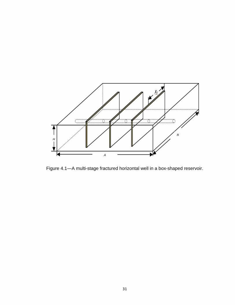
Figure 4.1 is a diagrammatic representation of a multi-stage fractured
horizontal well in a box-shaped reservoir. In order to derive a semi-analytical
model, the following assumptions are made:
The fractured horizontal well is located in a homogeneous box-shaped
reservoir. All the boundaries are closed boundaries.
The model is derived for single-phase flow.
The fluid flow from the reservoir directly to the horizontal wellbore is
considered.
The reservoir could be isotropic or anisotropic.
The horizontal wellbore is parallel to reservoir boundaries.
31
Figure 4.1―A multi-stage fractured horizontal well in a box-shaped reservoir.
A
B
H
32
The fractures are vertical, symmetrical and perpendicular to the horizontal
well. Each hydraulic fracture is equally spaced along the horizontal well.
If the reservoir is anisotropic, the geometric mean of permeabilities from
three dimensions is chosen as the reference permeability. Additionally, the
hydraulic fractures are not necessarily assumed to be the same in properties.
However, creating equally spaced hydraulic fractures with similar properties is a
common practice unless there is significant difference among fractures in field
application. Furthermore, it is very difficult to discern individual fracture
properties from transient pressure data alone (Raghavan et al, 1997).
4.1.1 Dimensionless variables
At first, I will define the dimensionless pressure and time as
Bq
ppkhp
sc
i
D
, ············································································ (4.1)
and
2
rt
D
LC
ktt
, ················································································· (4.2)
where
3zyx
kkkk . ·················································································· (4.3)
In Equations (4.1), (4.2), and (4.3), Lr means a reference length and k becomes
reference permeability.
To consider variable gas compressibility cg (p) and viscosity μ (p) in gas wells’
transient pressure analysis, the adjusted pressure can be used (Olarewaju and
Lee, 1989):
33
dpp
pp
p
pr
r
ar
)(
)(
, ········································································· (4.4)
where pr is a reference pressure and μr and ρr are the viscosity and density
under the reference pressure. Usually, the standard pressure is taken as the
reference pressure.
As Agarwal (1979) indicated, when analyzing build-up test results, it is
useful to make time transformations. However, for drawdown tests, there is no
such need.
The dimensionless distances in x-, y-, and z-direction are defined as
xr
D
k
k
L
xx , ·················································································· (4.5)
yr
D
k
k
L
yy , ············································································ (4.6)
and
zr
D
k
k
L
zz , ············································································· (4.7)
For the hydraulic fracture system, the dimensionless fracture conductivity
and fracture diffusivity are defined as
r
ff
fD
kL
wkC , ············································································· (4.8)
and
k
C
C
kC
t
tff
f
, ·········································································· (4.9)
34
respectively, where kf is the fracture permeability and Ctf is the fracture total
compressibility.
The dimensionless flow rates are expressed as :
Q
f
fD , ················································································· (4.10)
Q
Lqq
rrf
rfD , ·············································································· (4.11)
Q
Lqq
rrh
rhD . ············································································· (4.12)
4.1.2 Mathematical model
The mathematical model depicting the fluid flow in a reservoir with a
fractured horizontal well consists of three parts: (1) the fluid flow in the formation,
(2) the flow in the fracture, and (3) the pipe flow in the wellbore (Pipe flow will be
discussed in the next section). Fractures are regarded as plane sources with
non-uniform flux distribution. Compared with the whole reservoir, the horizontal
wellbore is considered to be a line source.
The equation describes the pressure drop in the formation as
t
pC
z
p
y
p
x
pk
t
2
2
2
2
2
2
. ······················································ (4.13)
For fractures, the inner boundary conditions is
),( tyqx
pkh
rf
xxF
,
ff
yyy ··················································· (4.14)
and the initial condition
iptzyxp )0,,,( . ····································································· (4.15)
35
For the horizontal wellbore, the inner boundary condition is expressed as
)(2
2,
tqr
prk
rhH
zrrw
, ······························································ (4.16)
and the outer boundary conditions can be written as
0),,,(
x
tzyxp, at 0x or Ax , ·················································· (4.17)
0),,,(
y
tzyxp, at 0y or By , ················································· (4.18)
0),,,(
z
tzyxp, at 0z or Hz . ·················································· (4.19)
The mathematical model for the pressure drop inside fractures can be derived
as
t
pC
hw
tyq
y
pkf
tff
f
rfff
,
2
2
, ······················································ (4.20)
And the boundary conditions as,
hBy
fpp
2
··············································································· (4.21)
0
f
yy
f
y
p ·············································································· (4.22)
and initial condition as
ifptyp )0,( . ········································································ (4.23)
The dimensionless mathematical model for fluid flow in the formation is
represented as
D
D
D
D
D
D
D
D
t
p
z
p
y
p
x
p
2
2
2
2
2
2
, ·························································· (4.24)
36
With the inner boundary conditions,
),(DDDrf
xxD
Dtyq
x
p
DFD
,
fDDfD
yyy ······································ (4.25)
DrhD
D
HzrrD
D
Dtq
H
r
pr
DDwDD
22
,
, ··················································· (4.26)
and the outer boundary conditions,
0
D
D
x
p, at 0
Dx or
DDAx , ······················································· (4.27)
0
D
D
y
p, at 0
Dy or
DDBy , ······················································ (4.28)
0
D
D
z
p, at 0
Dz or
DDHz . ······················································ (4.29)
and the initial condition,
0)0,,,( DDDDD
tzyxp , ······························································ (4.30)
The corresponding dimensionless equations for flow inside hydraulic
fractures can be reformulated as
D
fD
fD
rfD
D
fD
t
p
CC
q
y
p
1
2
2
, ······························································ (4.31)
and boundary conditions,
hDBy
fDpp
D
D
2
·········································································· (4.32)
0
DfD
yyD
fD
y
p··········································································· (4.33)
and initial condition,
37
0)0,( DDfD
typ . ······································································ (4.34)
4.1.3 Algorithm
A multi-stage fractured horizontal well in a box-shaped reservoir is
separated into four sub-systems: formation/fracture sub-system,
formation/horizontal well sub-system, fracture sub-system, and horizontal
wellbore sub-system. Each sub-system is discretized and solved individually in
Laplace domain. As such, the solutions for the above sub-systems in Laplace
domain are coupled based on the interface pressure- and flux-continuity
conditions. Finally, Stehfest’s (1970) Laplace inversion algorithm is applied to
determine the corresponding pressure distribution in the real-time domain.
4.1.3.1 Fracture sub-system solution
In this fracture sub-system, each hydraulic fracture is supposed to have a
finite-conductivity. Fluid flow in the fractures is simplified as 1D linear flow, which
is similar to fractured vertical wells. Furthermore, each hydraulic fracture is
discretized into equal segments. In each segment, fluid flows from the reservoir
qrf beside the inside flow qf (Figure 4.2a). At interfaces between adjacent
segments, solutions are coupled with equal flow rate and pressure.
Based on the results of Van Kruysdijk (1988), the dimensionless pressure at
xD (xDi-1 <xD < xDi) in Laplace domain for segment i is (Van Kruysdijk, 1988):
rfDiifDiifDiiDfDiqCqBqAuxp
1),( , ni 1 ··································· (4.35)
where

38
Cuxx
Cuxx
DiD
fD
i
DiD
DiD
e
e
Cuxx
CuC
A
)(
)(2
11
1
1
cosh21
, ················· (4.36)
Cuxx
Cuxx
DDi
fD
i
DDi
DDi
e
e
Cuxx
CuC
B
)(
)(2
1
cosh21
, ···················· (4.37)
uC
CC
fD
i
. ·············································································· (4.38)
In this case, u is the Laplace variable.
Usually, choked fracture skin effect refers to the presence of a damaged
near-wellbore zone with a reduced conductivity in a hydraulic fracture (Romero
et al., 2003). The extra pressure drop caused by the choked skin factor sck can
be expressed as:
u
sp
ck
D , ··············································································· (4.39)
And (Romero et al., 2003)
1,ckf
f
f
ck
ckk
k
x
xs
, ···································································· (4.40)
where kf, ck is the choked fracture permeability and xck is length of the choked
zone.
4.1.3.2 Horizontal well sub-system solution
In previous papers (Babu and Odeh, 1988; Ozkan et al., 2009), the
horizontal wellbore is always simplified as an infinite-conductivity “pipe”. In this
work, the wellbore pressure drop, which has never been included in fractured

39
(a)
(b)
(c)
Figure 4.2―Diagram showing fracture and horizontal wellbore discretization.
qout qin
qr

40
horizontal well model before, is discussed in detail. The pressure drop is the
result of frictional, radial influx and accelerational effects. The wellbore is divided
into m segments as shown in Figure 4.2b. Center points of each segment are
taken as the reference nodes among which the pressure drops are calculated.
The frictional pressure loss ∆pfric can be calculated as (Brown, 2003):
2
2v
d
Lfp
fric
, ······································································ (4.41)
where f is friction factor and v is fluid velocity. The friction factor is the explicit
approximation of the implicit Colebrook-White friction factor (Swamee and Jain,
1976).
Fluid flow directly from the reservoir and hydraulic fractures would cause a
pressure drop in the horizontal wellbore. Ouyang et al. (1996) proposed that the
radial influx effect could be incorporated with the frictional effect by introducing a
modified friction factor f*. For laminar flow, I have
6142.0
Re,
Re
*4303.01
64
wN
Nf , ·························································· (4.42)
and for turbulent flow (Ouyang et al., 1996),
3978.0
Re,0
*0153.01
wNff , ···························································· (4.43)
where f0 is the friction factor without consideration of the radial influx and
NRe,w=qrρ/πμ is the inflow Reynolds number. It is clear that the influx rate can
increase the pressure drop in the laminar flow regime. Conversely, pressure
drop is reduced in turbulent flow.
From the horizontal well toe to heel, fluid velocity keeps increasing, and this
accelerational effect causes an extra pressure drop. For each segment, the
41
pressure drop caused by the accelerational effect can be expressed as a
function of the change in momentum ∆M:
)(22
inoutaccvv
A
Mp
. ·························································· (4.44)
Here vin and vout are fluid flow velocities into and out of the wellbore segment,
respectively.
The total pressure drop is the sum of the aforementioned three kinds of
pressure loss. Then, the total pressure loss is converted into Laplace domain by
dividing the Laplace variable u.
4.1.3.3 Formation/Fracture and Formation/Horizontal Well Sub-system
Solutions
The source function method is effective in dealing with a wide variety of
reservoir flow problems. Instantaneous source functions proposed by Gringarten
and Ramey (1973) are applied in this paper. Compared with the whole reservoir,
each hydraulic fracture segment with unit source strength can be treated as a
finite vertical plane source that can be written as the intersection of an infinite
slab source and an infinite plane source in infinite slab reservoirs:
0
),(D
ut
yxDDdteSSuyp D . ··························································· (4.45)
where
1
2
22)(
exp
)(cos
)(cos
11
n
D
DD
D
DD
D
DD
x
A
tn
A
xxn
A
xxn
AS
, ······················· (4.46)
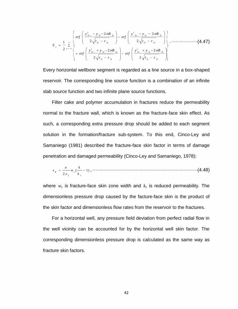
42
n
DD
DDD
DD
DDD
DD
DDD
DD
DDD
y
t
nByyerf
t
nByyerf
t
nByyerf
t
nByyerf
S
2
2
2
2
2
2
2
2
2
1 . ················· (4.47)
Every horizontal wellbore segment is regarded as a line source in a box-shaped
reservoir. The corresponding line source function is a combination of an infinite
slab source function and two infinite plane source functions.
Filter cake and polymer accumulation in fractures reduce the permeability
normal to the fracture wall, which is known as the fracture-face skin effect. As
such, a corresponding extra pressure drop should be added to each segment
solution in the formation/fracture sub-system. To this end, Cinco-Ley and
Samaniego (1981) described the fracture-face skin factor in terms of damage
penetration and damaged permeability (Cinco-Ley and Samaniego, 1978):
)1(2
s
s
f
ff
k
kw
xs
, ···································································· (4.48)
where ws is fracture-face skin zone width and ks is reduced permeability. The
dimensionless pressure drop caused by the facture-face skin is the product of
the skin factor and dimensionless flow rates from the reservoir to the fractures.
For a horizontal well, any pressure field deviation from perfect radial flow in
the well vicinity can be accounted for by the horizontal well skin factor. The
corresponding dimensionless pressure drop is calculated as the same way as
fracture skin factors.
43
4.1.3.4 Coupling the solutions
The solutions from different sub-systems are coupled together between any
two adjacent segments. For the pressure calculation in the horizontal wellbore,
unknown wellbore flow distribution becomes necessary when coupling solutions.
Therefore, a hypothetical uniform initial flow distribution along the wellbore and
an iterative process are applied in the model. The procedure of coupling all
solutions to generate a linear equation system is shown in Figure 4.3.
4.2 Model validation
KAPPA Ecrin, a commercial well-testing software, verified my model. The
wellbore pressure drop cannot be considered in KAPPA analytical models.
Therefore, results without horizontal wellbore pressure drops from my work were
compared with those obtained from KAPPA Ecrin. Figure 4.4 shows the
comparison of the two methods for a horizontal well with four identical hydraulic
fractures. The input parameters also appear in this figure.
The comparison suggests the results from this work are consistent with the
results from the commercial software. As expected, there are four flow regimes
for the multiple-fracture system in Figure 4.4: bilinear/linear flow, early-radial
flow, compound-linear flow (CLF), and pseudo-radial flow, which is similar with
the conclusion of Chen and Raghavan (1997). Therefore, the mathematical
model and its algorithm are reliable. Moreover, it is difficult to track the early-
time pressure behaviour in KAPPA Ecrin. However, the model provided here
can provide very early-stage pressure behaviour and guarantee accuracy.
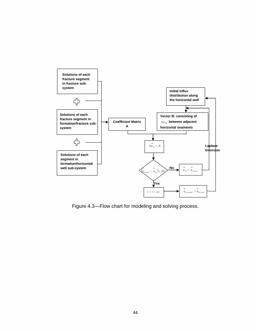
44
Figure 4.3―Flow chart for modeling and solving process.
newDDqq
,
ebsqqDnewD
,
No
Laplace
Inversion
BqAD
Initial influx
distribution along
the horizontal well
Vector B: consisting of
hDp between adjacent
horizontal segments
Coefficient Matrix
A
Solutions of each
fracture segment
in fracture sub-
system
Solutions of each
fracture segment in
formation/fracture sub-
system
Solutions of each
segment in
formation/horizontal
well sub-system
Yes
ttt newDinitialDqq
,,

45
Figure 4.4―Model validation with KAPPA Ecrin.
0.01
0.1
1
10
100
1E-6 1E-5 1E-4 1E-3 1E-2 1E-1 1E+0 1E+1 1E+2
Pw
D, d
Pw
D/d
lnt D
tD
This Work
Kappa Results
rw 0.05m h 50 m porosity 0.2 viscosity 0.001Pa.s Q 100 m3/day k 0.004mD Xf 50m kfwf 6×10-12m3

46
4.3 Results and discussion
4.3.1 Effect of fluid flow from reservoir to horizontal wellbore
Figure 4.5 compares the pressure behaviour with and without the
contribution of the horizontal wellbore for 3-, 10-, and 20-stage fractured
horizontal wells, respectively. Correspondingly, 3, 10, and 20 are the stage
numbers for these fractured horizontal wells. Here, wellbore pressure drops
were not taken into consideration. Fluid flow directly from the reservoir could blur
the differentiation between bilinear/linear and early-radial flow when stage
number was small. Moreover, fluid flow directly from the reservoir reduces the
pressure drop slightly until the pseudo-steady-state (PSS) regime is reached.
Horizontal wellbore contributions are weakened greatly when more fractures
are created. A reasonable explanation can be found by comparing fracture
contributions to the total production. Figure 4.6 shows the production proportion
of fractures and the horizontal wellbore to the total production. The upper lines
correspond to fractures while the lower ones are for wellbores. Contributions
from a horizontal wellbore increase over time. In fact, the ratio increases from
0.09 to 0.33 for a 3-stage fracture horizontal well. Although a horizontal wellbore
produces more oil, fractures produce much more fluids than wellbores. This
phenomenon becomes more evident when the fracture stage number increases
to 20; at that level, the fracture production ratio remains around 0.99. Actually,
the stages of some open-hole multi-stage fractured horizontal wells can reach
more than 20. Therefore, the flow directly into the wellbore can be ignored when
the stage number for a fractured horizontal well is large enough.
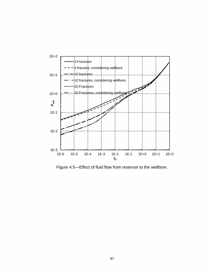
47
Figure 4.5―Effect of fluid flow from reservoir to the wellbore.
1E-3
1E-2
1E-1
1E+0
1E+1
1E+2
1E-6 1E-5 1E-4 1E-3 1E-2 1E-1 1E+0 1E+1 1E+2
Pw
D
tD
3 Fractures
3 fracutes, considering wellbore
10 fractures
10 fractures, considering wellbore
20 Fractures
20 Fractures, considering wellbore
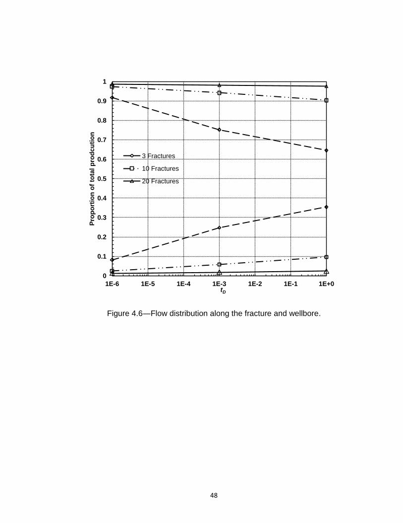
48
Figure 4.6―Flow distribution along the fracture and wellbore.
0
0.1
0.2
0.3
0.4
0.5
0.6
0.7
0.8
0.9
1
1E-6 1E-5 1E-4 1E-3 1E-2 1E-1 1E+0
Pro
po
rtio
n o
f to
tal p
rod
cu
tio
n
tD
3 Fractures
10 Fractures
20 Fractures
49
4.3.2 Effect of horizontal wellbore pressure drop
Figure 4.7 compares the pressure behaviour from a 6-stage fractured
horizontal well under different production rates and reservoir permeabilities
(k=400 md, 40 md and 0.4 md). The pressure loss along the horizontal wellbore
can increase the early-stage pressure drops slightly but only when reservoir
permeability becomes large enough (k>100 md). Certainly the conclusion would
be different under low-permeability condition. There is no significant difference
between pressure drops—with and without considering wellbore pressure loss—
when permeability is less than 1 md. Furthermore, a higher production rate can
increase the pressure deviation if considering the wellbore pressure drop.
Similarly, when production rate is high but permeability is very low, the
drawdown ratio ( 0.36 kPa with wellbore contribution vs. 0.36 kPa without
wellbore contribution at k=0.4 mD) at t=0.001 day (Figure 4.7) is close to unit,
meaning it is the permeability rather than production rate that is the key
parameter that amplifies the horizontal wellbore pressure loss. For tight
formation and shale gas reservoirs, permeability is usually in the range of
microdarcies or below, and, as such, wellbore pressure loss has little influence
on the transient pressure behaviour. Therefore, the effect of pressure drops
inside the horizontal wellbore of multi-stage fractured horizontal wells can be
ignored in tight and shale formations.

50
(a)
(b)
Figure 4.7―Effect of horizontal wellbore pressure drop.
1E-2
1E-1
1E+0
1E+1
1E+2
1E+3
1E-4 1E-2 1E+0 1E+2
Pw
D, d
Pw
D/d
lnt D
tD
k=400md
k=40md
k=0.4md
Without horizontal well pressure drop
Q=100 m3/day
1E-2
1E-1
1E+0
1E+1
1E+2
1E+3
1E+4
1E-4 1E-3 1E-2 1E-1 1E+0 1E+1 1E+2 1E+3 1E+4
Pw
D, d
Pw
D/d
lnt D
tD
k=400md
k=40md
k=0.4md
Without horizontal well pressure drop
Q=1000 m3/day

51
4.3.3 Effect of fracture stages
For multi-stage fractured horizontal wells, fracture stages have significant
influence on productivity and economic benefits. Here, fracture stage effects
were analyzed in three steps without changing the fracture width.
4.3.3.1 Constant fracture half-length
Figure 4.8 gives the pressure responses and their logarithmic derivatives
with different fracture stages and the same fracture half-lengths for a 600 m
horizontal well. Figure 4.9 presents the dimensionless relative productivity
indexes over time under different fracture numbers for the fractured wells. PSS
productivity index, J, has been accepted as a criterion for evaluating fracture
performance, whose dimensionless form is defined as (Zeng, 2008):
wfD
D
pJ
1 , ···············································································(4.49)
where pwfD is the dimensionless flowing bottomhole pressure.
According to Figures 4.8 and 4.9, a larger stage number makes a larger
total fracture volume, which leads to less pressure drop and higher productivity.
Such well productivity increment decreases with increasing fracture stages while
also increasing multi-stage fracturing cost. Hence, optimum fracture stage
numbers (fracture spacing) must exist under constant fracture half-lengths .
In Figure 4.9, the wells’ productivities are linearly related to the fracture
numbers in the early-stage production. For example, the 40-stage fractured
horizontal well works as well as 40 separate fractured vertical wells in the
bilinear/linear flow regime. Therefore, to analyze early-time pressure data of
52
fractured horizontal wells, a conventional analysis method for bilinear/linear flow
can be easily applied.
After the bilinear/linear flow, interference between fractures appears. The
duration of bilinear/linear flow becomes shorter and interference appears earlier
with more fractures along the wellbore. In fact, when the number of fractures
increases to 40, pressure and pressure derivative curve slopes are close to units
in the interference period after tD=0.002. This apparent BDF is similar to the PSS
flow. In fact, this phenomenon means the appearance of SRV. The key
parameter controlling SRV is the ratio of the fracture spacing and fracture half-
length. When the fracture spacing is significantly smaller than the half-length,
SRV appears clearly.
4.3.3.2 Constant total fracture volume
Figure 4.10 compares the pressure and corresponding derivative curves
under the constant total fracture volume. Figure 4.11 provides the relative
productivity index as it changes over fracture stages and time. As shown in
Figures 4.10 and 4.11, the pressure drop is reduced with more fractures in early-
stage production while productivity growth tends to slow down. Correspondingly,
more fractures will cause a high production rate if the bottomhole pressure (BHP)
is constant.
The appearance of SRV reverses such a trend. For example, the
dimensionless pressure derivative of the well with10 fractures tended to surpass
one with less than 10 fractures after tD=0.002. This suggests that the pressure
drop of a 10-stage fractured horizontal well increases more quickly than a well
53
with less than 10 fractures. Furthermore, the 10-stage fractured well’s
productivity would become lower than that of the 4-stage fractured horizontal
well (Figure 4.11). Therefore, in the long term, creating more fractures is not
always better. As discussed in 4.3.3.1, there also exists an optimum
combination of fracture stage and fracture half-lengths when the total fracture
volume remains constant.
4.3.3.3 Non-uniform fractures
For many, natural fractures in shale formations are critical in controlling
shale gas well productivity (Gaskari and Mohaghegh, 2006). Unpropped
fractures induced by hydraulic fracturing treatments can also exist alongside
pre-existing open natural fractures.
In Figure 4.12, I simply added small fractures beside each hydraulic fracture
to simulate natural and induced fractures for a 7-stage fractured horizontal well.
These seven hydraulic fractures have different lengths. At first, 7 small fractures
were added on the right of hydraulic fractures as natural/induced fractures. Then,
another 7 larger fractures were created. Each natural/induced fracture can have
different half-lengths and conductivities but, for the sake of simplicity, 7 small
and 7 larger natural/induced fractures possessed similar properties.
Figure 4.13 shows the pressure responses of natural/induced fractures. It is
clear that natural/induced fractures work as if improving hydraulic fracture
conductivities. So, the hydraulic fracture conductivity can be overestimated if
existing natural/induced fractures are ignored. However, it is difficult to estimate

54
natural/induced fractures with only transient pressure behaviour data shown in
Figure 4.13.
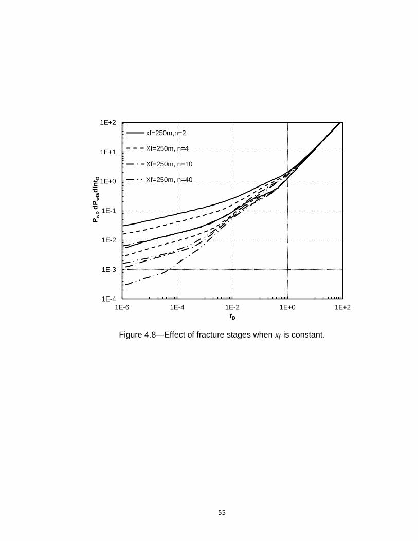
55
Figure 4.8―Effect of fracture stages when xf is constant.
1E-4
1E-3
1E-2
1E-1
1E+0
1E+1
1E+2
1E-6 1E-4 1E-2 1E+0 1E+2
Pw
D d
Pw
D/d
lnt D
tD
xf=250m,n=2
Xf=250m, n=4
Xf=250m, n=10
Xf=250m, n=40
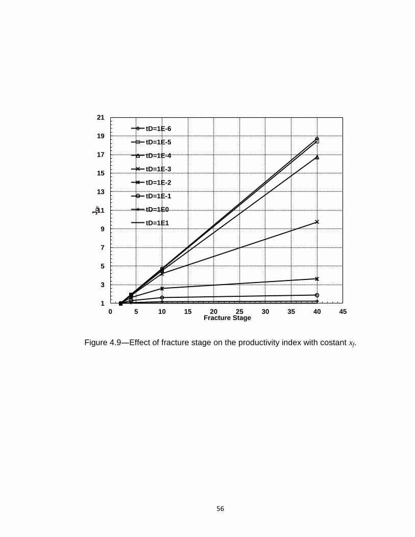
56
Figure 4.9―Effect of fracture stage on the productivity index with costant xf.
1
3
5
7
9
11
13
15
17
19
21
0 5 10 15 20 25 30 35 40 45
JD
r
Fracture Stage
tD=1E-6
tD=1E-5
tD=1E-4
tD=1E-3
tD=1E-2
tD=1E-1
tD=1E0
tD=1E1

57
Figure 4.10―Effect of fracture stages when fracture volume is constant.
1E-3
1E-2
1E-1
1E+0
1E+1
1E+2
1E-6 1E-5 1E-4 1E-3 1E-2 1E-1 1E+0 1E+1 1E+2
Pw
D
dln
Pw
D/d
lnt D
tD
Xf=250,n=2
Xf=167,n=3
Xf=125,n=4
Xf=100, n=5
Xf=83,n=6
Xf=71,n=7
Xf=62.5,n=8
Xf=55.5,n=9
Xf=50,n=10

58
Figure 4.11―Effect of fracture stages on the productivity indxex with cosntant Vf.
0.8
1
1.2
1.4
1.6
1.8
2
2.2
2.4
2.6
0 2 4 6 8 10 12
JD
r
Fracture Stages
tD=1E-6
tD=1E-5
tD=1E-4
tD=1E-3
tD=1E-2
tD=1E-1
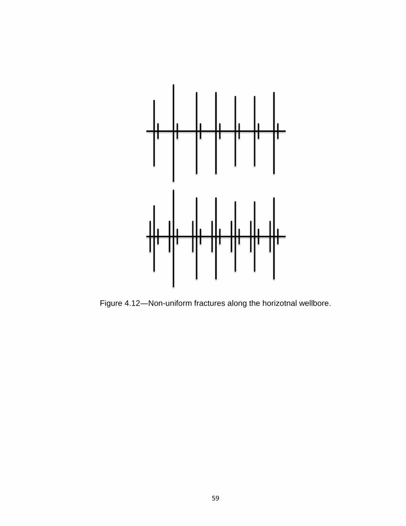
59
Figure 4.12―Non-uniform fractures along the horizotnal wellbore.
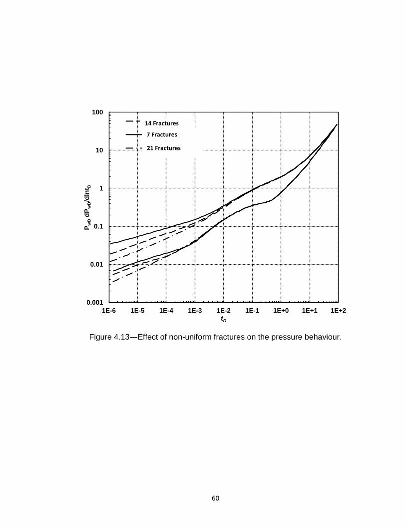
60
Figure 4.13―Effect of non-uniform fractures on the pressure behaviour.
0.001
0.01
0.1
1
10
100
1E-6 1E-5 1E-4 1E-3 1E-2 1E-1 1E+0 1E+1 1E+2
Pw
D d
Pw
D/d
lnt D
tD
Series1
Series3
Series5
7 Fractures
14 Fractures
21 Fractures
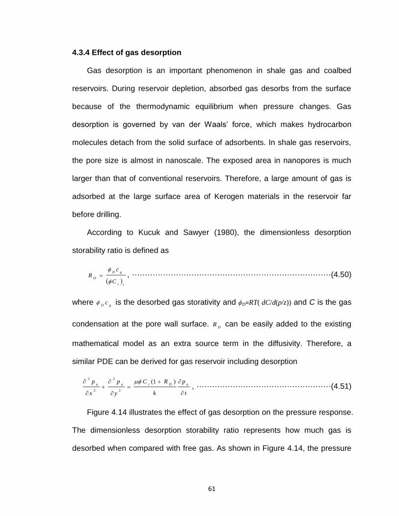
61
4.3.4 Effect of gas desorption
Gas desorption is an important phenomenon in shale gas and coalbed
reservoirs. During reservoir depletion, absorbed gas desorbs from the surface
because of the thermodynamic equilibrium when pressure changes. Gas
desorption is governed by van der Waals’ force, which makes hydrocarbon
molecules detach from the solid surface of adsorbents. In shale gas reservoirs,
the pore size is almost in nanoscale. The exposed area in nanopores is much
larger than that of conventional reservoirs. Therefore, a large amount of gas is
adsorbed at the large surface area of Kerogen materials in the reservoir far
before drilling.
According to Kucuk and Sawyer (1980), the dimensionless desorption
storability ratio is defined as
tt
gD
D
C
cR
, ············································································· (4.50)
where gD
c is the desorbed gas storativity and ϕD=RT( dC/d(p/z)) and C is the gas
condensation at the pore wall surface. D
R can be easily added to the existing
mathematical model as an extra source term in the diffusivity. Therefore, a
similar PDE can be derived for gas reservoir including desorption
t
p
k
RC
y
p
x
paDtaa
)1(
2
2
2
2
, ···················································· (4.51)
Figure 4.14 illustrates the effect of gas desorption on the pressure response.
The dimensionless desorption storability ratio represents how much gas is
desorbed when compared with free gas. As shown in Figure 4.14, the pressure

62
drop with gas desorption is lower than without desorption. As a result, gas
desorption acts as an extra source in the reservoir and puts off the appearance
of BDF.
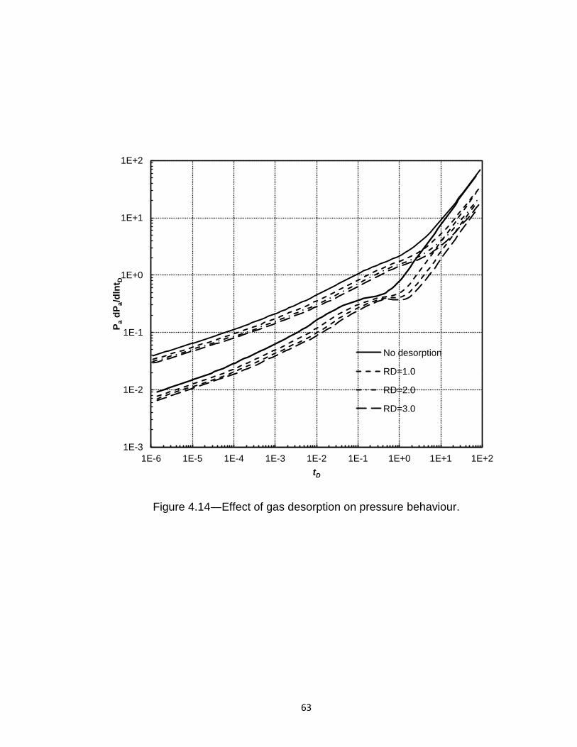
63
Figure 4.14―Effect of gas desorption on pressure behaviour.
1E-3
1E-2
1E-1
1E+0
1E+1
1E+2
1E-6 1E-5 1E-4 1E-3 1E-2 1E-1 1E+0 1E+1 1E+2
Pa d
Pa/d
lnt D
tD
No desorption
RD=1.0
RD=2.0
RD=3.0
64
4.3.5 Effect of skin factors
Figure 4.15 shows pressure and derivative curves with different skin factors
for a 3-stage fractured horizontal well. Here, I assumed that the skin factors
along fractures and the wellbore remain constant. Actually, I can generate the
pressure data for varying skin factors. However, I cannot discern different skin
factors along fractures and along the wellbore in field application. In Figure 4.15,
fracture choked skin factor sck increases the pressure drop significantly and is
followed by the fracture face-skin factor sff. With the same skin factor value, the
horizontal well skin factor sh only increases the dimensionless pressure a little.
The surface area of fractures is much larger than in the horizontal wellbore and
most of the fluid flows to the wellbore through fractures. Therefore, relatively
small fracture skin factors can make a more significant difference than the same
horizontal wellbore skin factors. Moreover, fracture-face skin factors can mask
the bilinear/linear flow regime and make it difficult to catch bilinear/linear flow in
log-log plots of pressure and pressure derivatives.
Figure 4.16 compares the flow distribution with different skin factors at
tD=10-6. The effect of fracture-face skin factor seems more complex than the
choked skin factor. The fracture-face skin factor reduces the amount of fluid
from the reservoir to fractures and increases pressure drops. Moreover, the
fracture-face skin factor tries to reduce the influx difference to reach an even
flow distribution along fractures.
The choked skin factor increases the pressure drop inside fractures since
the choked skin factor reduces the conductivities of fractures in the vicinity of the
65
well. Also, the choked skin factor reduces the amount of fluid influx from the
reservoir to fractures. However, it has no influence on the influx distribution
pattern along fractures. Obviously, the horizontal well skin factor also has little
influence on the influx along fractures.
As far as the total skin factor is concerned, the extra pressure drop is not
equal to the sum of the extra pressure drop caused by each skin factors.
Ultimately, different skin factors can interact with each other and finally strike a
balance.
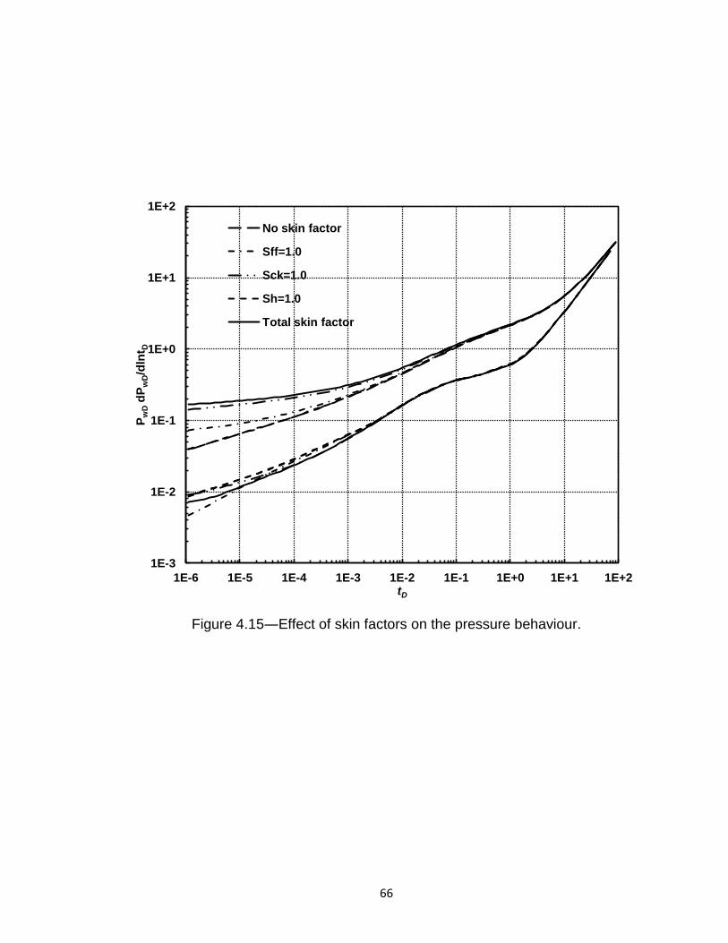
66
Figure 4.15―Effect of skin factors on the pressure behaviour.
1E-3
1E-2
1E-1
1E+0
1E+1
1E+2
1E-6 1E-5 1E-4 1E-3 1E-2 1E-1 1E+0 1E+1 1E+2
Pw
D d
Pw
D/d
lnt D
tD
No skin factor
Sff=1.0
Sck=1.0
Sh=1.0
Total skin factor

67
Figure 4.16―Effect of skin factors on the flow distribution along the fracture.
0.00
0.02
0.04
0.06
0.08
0.10
0.12
0.14
0.0 0.2 0.4 0.6 0.8 1.0
qrf
D
XfD
No skin factor
Sff=1.0
Sck=1.0
Sh=1.0
Total skin factor
tD=1E-6

68
4.4 Field examples
Using my model, I performed a pressure transient analysis based on field
data. The well is a multi-stage fractured horizontal well in a typical shale gas
reservoir in Sichuan, China. The pressure data came from two build-up tests
after almost one-year production. Figure 4.17 shows the gas production rates
from August 2, 2011, to May 30, 2012. Table 4.1 summarizes the basic input
parameters for this example.
4.4.1 No.1 Build-up test analysis
At first, I completed a qualitative type-curve analysis. Since the duration of
the 1st build-up test is short and the reservoir permeability is extremely low, I
found no characteristic pressure responses such as half-slope trend in CLF and
the unit-slope line at late times. In addition, I cannot detect the fracture half-
length directly from the plot of ∆pa―t1/2 because no linear-flow trend appears in
the build-up test. However, what I can distinguish from the log-log plot is the
bilinear flow. Accordingly, I plotted ∆pa vs. t1/4
in Figure 4.18. The slope of the
straight line through the data is m=90 MPa/hr1/4. Using this slope, I estimated the
fracture conductivity wfkf =2.88×10⁻¹⁵ m3.
Next, I compared the real field data with different type curves to find the
most appropriate fracture half-length and fracture conductivity. Figure 4.19
shows the matching results with my model. In general, the match is satisfactory.
I chose a constant value Cw=9.20×10⁻⁶ m3/Pa (0.4 bbl/psi) to account for the
wellbore storage effect. In fact, in Figure 4.19, I can see that the wellbore
storage factor is not strictly constant and varies from 7×10⁻⁶ to 1×10⁻⁵ m3/Pa (0.3
69
to 0.5 bbl/psi) during the build-up test. Furthermore, the fracture half-length was
estimated as 137 m and the fracture conductivity was 4×10-16 m3. This is the
best match for the whole data set. As such, I can also conclude that the area of
the SRV should be 67.7 acres (L×2 x f =274000 m2). In fact, the fracture
conductivity is not as good as the one shown in my type curve. Higher fracture
conductivity can make the pressure derivative bend upward with a greater angle
as seen at the end of this test. However, in Figure 4.19, the derivative is almost
flat at the end. Therefore the fracture conductivity should be a little lower than
my expectation.
4.4.1 No.2 Build-up test analysis
After analyzing the No.1 build-up test, I recognized that using specific lines
to evaluate fractures is limited for shale gas wells. Thus, I directly employed the
type curve matching method to conduct quantitative analysis for the No.2 build-
up test. Figure 4.20 shows the matching results with my model. In this case, the
wellbore storage factor increases to 2.3×10⁻⁵ m3/Pa (1.0 bbl/psi), while the
average fracture’s half-length was estimated as 100 m. Moreover, its
conductivity was recalculated as 6.2×10⁻¹⁶ m3. Compared to the No.1 analysis
results, the half-length is shorter and conductivity is higher. This is reasonable.
In fact, part of the proppant flows back to the wellbore along with gas; therefore
the corresponding fracture section is almost closed without proppant support,
but the remaining part of the fracture swells after extra proppant squeezes in.

70
Figure 4.17―Field production data.
0
2000
4000
6000
8000
10000
12000
14000
16000
0 1000 2000 3000 4000 5000 6000 7000
Pro
du
ctio
n r
ate
, m3 /
Day
Time,hr
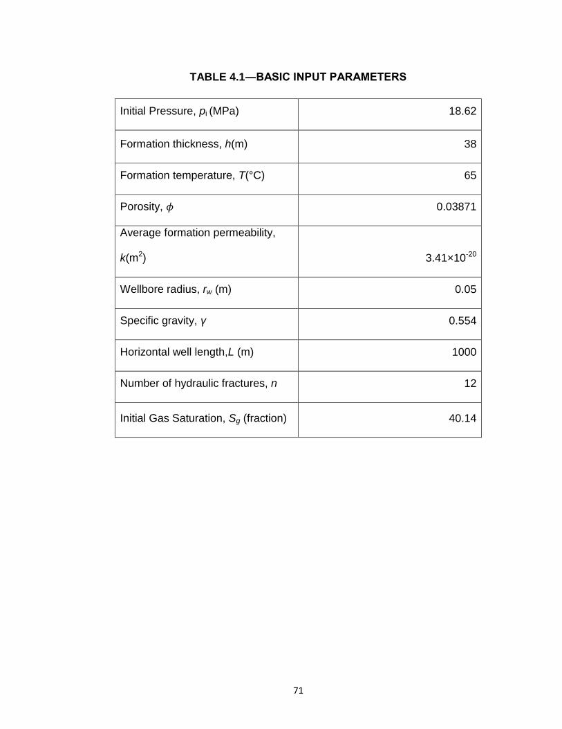
71
TABLE 4.1―BASIC INPUT PARAMETERS
Initial Pressure, pi (MPa) 18.62
Formation thickness, h(m) 38
Formation temperature, T(°C) 65
Porosity, 0.03871
Average formation permeability,
k(m2) 3.41×10⁻²⁰
Wellbore radius, rw (m) 0.05
Specific gravity, γ 0.554
Horizontal well length,L (m) 1000
Number of hydraulic fractures, n 12
Initial Gas Saturation, Sg (fraction) 40.14
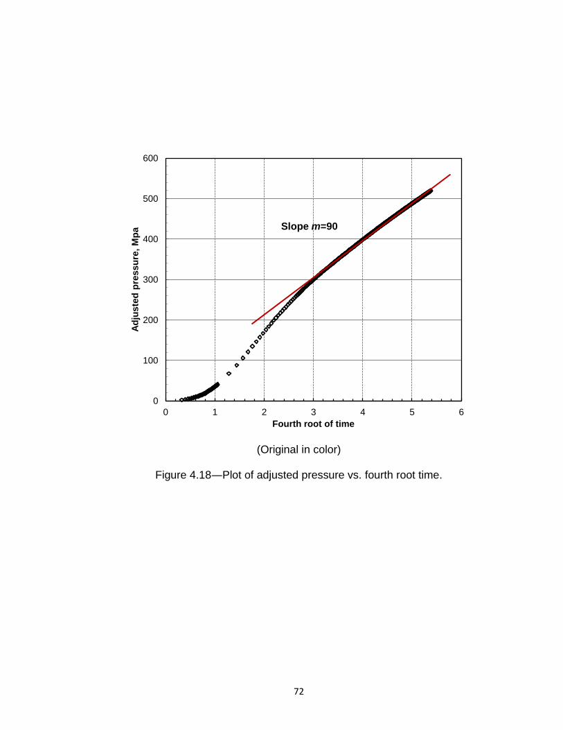
72
(Original in color)
Figure 4.18―Plot of adjusted pressure vs. fourth root time.
0
100
200
300
400
500
600
0 1 2 3 4 5 6
Ad
juste
d p
ressu
re,
Mp
a
Fourth root of time
Slope m=90
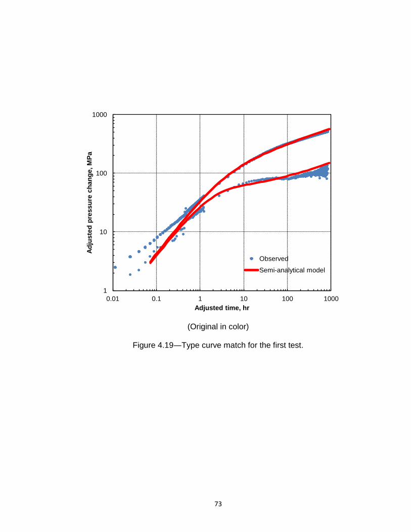
73
(Original in color)
Figure 4.19―Type curve match for the first test.
1
10
100
1000
0.01 0.1 1 10 100 1000
Ad
juste
d p
ressu
re c
han
ge,
MP
a
Adjusted time, hr
Observed
Semi-analytical model
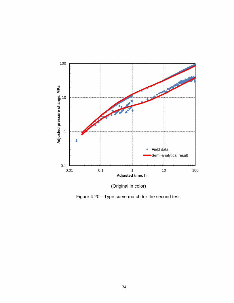
74
(Original in color)
Figure 4.20―Type curve match for the second test.
0.1
1
10
100
0.01 0.1 1 10 100
Ad
juste
d p
ressu
re c
han
ge,
MP
a
Adjusted time, hr
Field data
Semi-analytical result
75
4.5 Chapter summary
In this chapter, a semi-analytical model has been built to study the transient
pressure behaviour of multi-stage fractured horizontal wells in a rectangular
reservoir. The effect of different parameters on well production has been studied
in detailed. Several conclusions can be derived:
The model and its algorithm were validated to be applicable in transient
pressure analysis for the multi-stage fractured horizontal well. It can be
further extended to study dual-porosity reservoirs and reservoirs with
complex fractures.
The fluid flow directly from reservoir to horizontal wellbore can change the
early-stage pressure and its derivative if fewer fractures are created along
the wellbore (n is in the range of 2 to 10). The pressure drop along the
wellbore can be ignored for typical multi-stage fracture horizontal wells in
tight formations and shale gas reservoirs.
When fracture half length is constant, there exists an optimum fracture
stage number considering the increase of the well’s productivity. When
total fracture volume is constant, there is also an optimum fracturing
design to obtain the highest profit. Therefore, an optimum fracturing
treatment must exist if all the necessary parameters are considered.
Different kinds of skin factors influence the pressure behaviour in different
aspects. Among all skin factors, the choked skin factor is the most
damaging to fractured wells’ productivity.

76
In field applications, pressure response might not display any
characteristic flow behaviour at early times for shale-gas wells.
Techniques based on the slopes of characteristic lines might not be
guaranteed. Type curve matching can be a candidate for analyzing the
overall pressure behaviour with a model to obtain a better solution.
77
CHAPTER 5
HYDRAULICALLY FRACTURED WELLS WITH STRESS-
SENSITIVE CONDUCTIVITIES
This chapter aims to derive solutions for the non-linear mathematical model
and accordingly describe the pressure behaviour of fractured wells with stress-
dependent conductivities. A box-shaped homogeneous reservoir with all closed
boundaries is considered, and the fractured well is located at the center of the
reservoir. In order to simulate the well/reservoir system by a mathematical
model, a few assumptions must be made first:
1. The porous media is isotropic, homogeneous, and bounded with upper
and lower impermeable strata.
2. Reservoir parameters such as porosity ϕ and permeability k are kept
constant.
3. Both the reservoir and hydraulic fractures are filled with a single fluid,
which could be gas or slightly compressible fluid with constant viscosity.
4. All the hydraulic fractures are vertical, symmetric and fully penetrate the
formation. For the multi-stage fractured horizontal well, properties of each fracture
at the initial time are assumed to be identical.
5. The fluid flow in the system is subject to Darcy’s law and the fluid flow in
hydraulic fractures is described with the Forchheimer equation.
The fracture conductivity is determined by fracture width and fracture
permeability. Although fracture width wf changes during production, considering
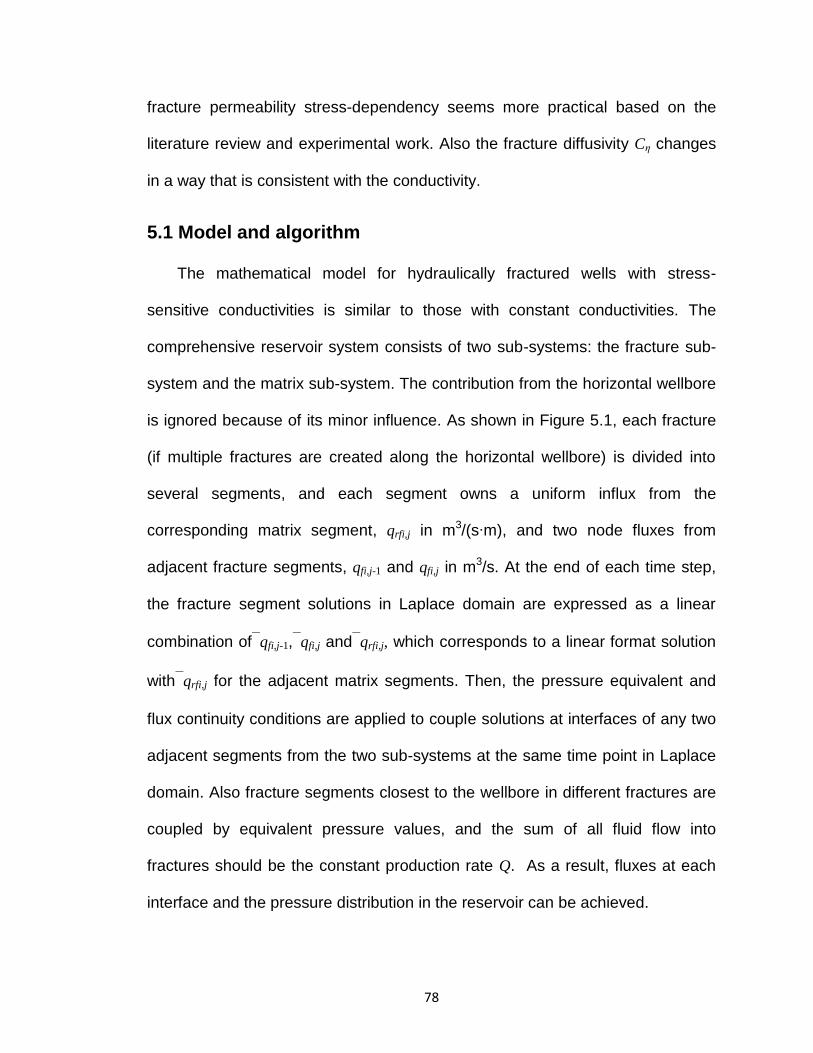
78
fracture permeability stress-dependency seems more practical based on the
literature review and experimental work. Also the fracture diffusivity Cη changes
in a way that is consistent with the conductivity.
5.1 Model and algorithm
The mathematical model for hydraulically fractured wells with stress-
sensitive conductivities is similar to those with constant conductivities. The
comprehensive reservoir system consists of two sub-systems: the fracture sub-
system and the matrix sub-system. The contribution from the horizontal wellbore
is ignored because of its minor influence. As shown in Figure 5.1, each fracture
(if multiple fractures are created along the horizontal wellbore) is divided into
several segments, and each segment owns a uniform influx from the
corresponding matrix segment, qrfi,j in m3/(s∙m), and two node fluxes from
adjacent fracture segments, qfi,j-1 and qfi,j in m3/s. At the end of each time step,
the fracture segment solutions in Laplace domain are expressed as a linear
combination ofqfi,j-1,qfi,j andqrfi,j, which corresponds to a linear format solution
withqrfi,j for the adjacent matrix segments. Then, the pressure equivalent and
flux continuity conditions are applied to couple solutions at interfaces of any two
adjacent segments from the two sub-systems at the same time point in Laplace
domain. Also fracture segments closest to the wellbore in different fractures are
coupled by equivalent pressure values, and the sum of all fluid flow into
fractures should be the constant production rate Q. As a result, fluxes at each
interface and the pressure distribution in the reservoir can be achieved.
79
However, the differences of such a stress-sensitive model from the model
with constant fracture conductivities are still obvious. For the fracture sub-
system, although each fracture’s conductivity remains constant during each time
step (Figure 5.2), they become different at different time steps. Meanwhile,
matrix properties remain unchanged at all times. This would cause a remarkable
difference in Laplace transformation for the above two sub-systems, which
brings challenges to coupling solutions on interfaces. Moreover, fracture
conductivities act as a function of stress/pressure, and stress/pressure is
influenced by fracture and reservoir characteristics in turn, which requires an
iterative process in modeling.
In order to couple fracture and reservoir sub-systems, the fracture sub-
system solutions with changing conductivities in Laplace domain should be
reformulated at first. For segment j of fracture i at time step k, I have
D
fD
fD
rfD
D
fD
Dt
p
CC
q
y
p
y
1 for
jDiDjDiyyy
,1,
,
k
DD
k
Dttt
1
············· (5.1a)
bounded with
jfDi
fDyyD
fDq
Cy
p
jDiD
,
1
,
1,
1
,1
jfDi
fDyyD
f
qCy
p
jDiD
D , ··························································· (5.1b)
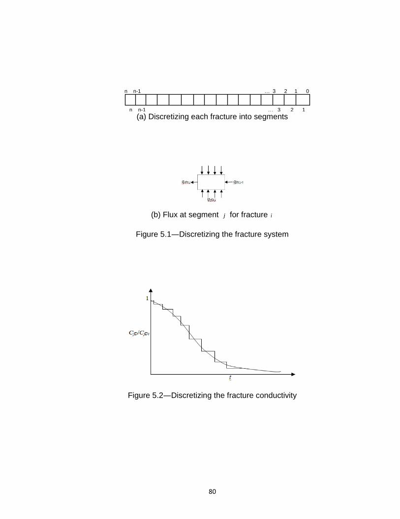
80
(a) Discretizing each fracture into segments
(b) Flux at segment j for fracture i
Figure 5.1―Discretizing the fracture system
Figure 5.2―Discretizing the fracture conductivity
n n-1 … 3 2 1 0
n n-1 … 3 2 1

81
and zero initial condition. The above mathematical model’s solution is obtained
as in Appendix B:
rfDiDji
jfDiDji
jfDiDjiD
jfDi qydqyCqybuyp*
,1,
*
,,
*
,,
*
)()()(),( , ··············· (5.2a)
where
Cuyy
Cuyy
jDiD
fD
Dji
jDiD
jDiD
e
e
Cuyy
CuC
yb
)(
)(2
,
,
,
,
1
])cosh[(21
)( ············ (5.2b)
Cuyy
Cuyy
DjDi
fD
Dji
DjDi
DjDi
e
e
Cuyy
CuC
yc
)(
)(2
1,
,
1,
1,
1
])cosh[(21
)( ········· (5.2c)
uC
Cd
fD
ji
,. ············································································ (5.2d)
In Equations (5.2a), (5.2b), (5.2c), and (5.2d), u’ is the Laplace variable forD
t .
The matrix sub-system solutions are the same as ones in the previous
model with constant properties. Then, solutions from two sub-systems in
different Laplace domains are coupled using methods mentioned in Chapter 3.
The next problem is to find the correlation between fracture conductivities
(which is defined by stress-dependent permeability) and stress/pressure. I chose
the simple but practical equation from Raghavan and Chin (2002) as shown
below:
ffffif
pd
fi
ppd
fifekekk
. ························································· (5.3)
In Equation (5.3), fi
k is the permeability at initial condition and f
d is the fracture
stress-sensitive characteristic. In fact, both the fracture conductivity f
C and
82
fracture diffusivity
C change when fracture permeability is stress-dependent.
Originally, Equation (5.3) was derived for rocks but was extended to modeling
hydraulic fractures by Berumen and Tiab (1996) and Pedroso et al. (1997). In
fact, my semi-analytical model can incorporate different stress-dependent
conductivity equations if other appropriate expressions are created. In the model,
I use the same df for each stage when the horizontal well is multi-stage fractured.
Furthermore, it is not realistic for the hydraulic fracture permeability to approach
zero, and, therefore, a minimum limit kfmin is set in the model.
The flux distribution and pressure distribution at each time step can be
mapped by coupling solutions and numerical inverse Laplace transformation,
which determines the fracture properties for next time step.
5.2 Model validation
The model and its algorithm were validated through comparison with two
limiting cases with constant fracture properties. The two cases in Figure 5.3
show the pressure behaviour of a 6-stage fractured horizontal well with initial
fracture conductivity CfD=10 and minimum conductivity CfDmin=0.5. The fracture
stress-dependent characteristic f
d was chosen to be 10-7 Pa-1. At the beginning,
pressure behaviour of the stress-sensitive case is consistent with the case
CfD=10. When the fracture conductivity reduces along with pressure, the
pressure behaviour deviates from the typical linear flow with a slope larger than
1/2. When CfD reaches the lowest value, the pressure derivative falls back to the
curve of CfD=0.5. This comparison suggests that the pressure behaviour
83
represented by this semi-analytical model changes gradually among the two
extreme cases, which provides indirect proof for the applicability of this model.
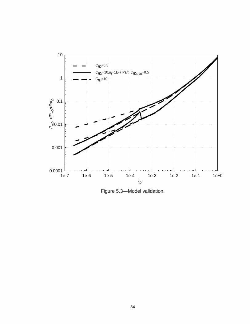
84
Figure 5.3―Model validation.
tD
1e-7 1e-6 1e-5 1e-4 1e-3 1e-2 1e-1 1e+0
Pw
D, dP
wD/d
lnt D
0.0001
0.001
0.01
0.1
1
10
CfD=0.5
CfDi=10,df=1E-7 Pa-1, CfDmin=0.5
CfD=10
85
5.3 Results and discussion
The pressure behaviour of stress-sensitive hydraulic fractures is
represented by following type curves with different combinations of variables.
The variables of interest included fracture conductivity Cf, the minimum fracture
conductivity CfDmin and stress-dependent characteristic df. Effects of these
variables on pressure behaviour were analyzed in detail. Table 5.1 lists the
properties of the fractured well, fluid, and formation used in section 5.3.
5.3.1 Pressure behaviour characteristics
Stress-sensitive hydraulic fracture conductivity’s existence has a significant
impact on the pressure behaviour of fractured wells. Figure 5.4 shows the
dimensionless wellbore pressure response and its derivative on a log-log plot
when fractures are stress-sensitive. At first, the stress-sensitive effect gradually
increases the wellbore pressure drop and pressure derivatives, which deviates
from typical flow regimes, especially bilinear/linear flow. When fracture
conductivity decreases as pressure drops, the slope of the linear flow regime
becomes increasingly higher than 1/2, which is the “signature” of linear flow
when fracture conductivity is constant. Likewise, the slope of bilinear flow
becomes larger than 1/4. Moreover, it should be noted that the amount of the
slope’s increase varies according to different combinations of parameters. If the
fracture conductivity changes rapidly, the wellbore pressure derivative curves
might display a slope that is close to or even larger than unit and/or overstrides
corresponding pressure curves, which can be considered as apparent BDF. This
conclusion is consistent with Berumen and Tiab’s work (1996). This special

86
feature can be considered as a sign of severe fracture conductivity reduction
during production.
When the fracture conductivity reduces to CfDmin and remains constant, the
pressure curve falls back to that with constant conductivity CfD=CfDmin, and,
therefore, pressure derivative has a rapid decline and a hump forms. As shown
in Figures 5.3 and 5.4, the sudden drop appears at the downward section of the
hump in pressure derivative curves, which is caused by the sudden conductivity
change at CfD=CfDmin. In order to eliminate the sudden drop in the pressure
derivative curve, I divided the CfD vs. P into three parts and each part is
described by a specific equation to smooth the conductivity curve. Figure 5.5
gives the smooth conductivity curve and original one. It shows that conductivity
gradually reduced to the minimum conductivity without sudden change in the
smooth conductivity curve.
Figure 5.6 shows the dimensionless pressure and pressure derivative
curves based on the smooth conductivity change in Figure 5.5. The sudden drop
is replaced by a slowly varying downward section in Figure 5.6, which means
that the derivative curve is smooth as long as the conductivity changes gradually.
In Figures 5.5 and 5.6, I applied a new conductivity model that is more
complex than Equation (5.3). But these new equations for CfD vs. P which aim at
smoothing the conductivity change are hypothetical. Large amount of accurate
experimental data are necessary to get reliable new equations for the smooth
conductivity change. Therefore, Equation (5.3) would still be used in the

87
following discussions to describe the stress-sensitive conductivity behavior until
new equations are obtained in the future work.
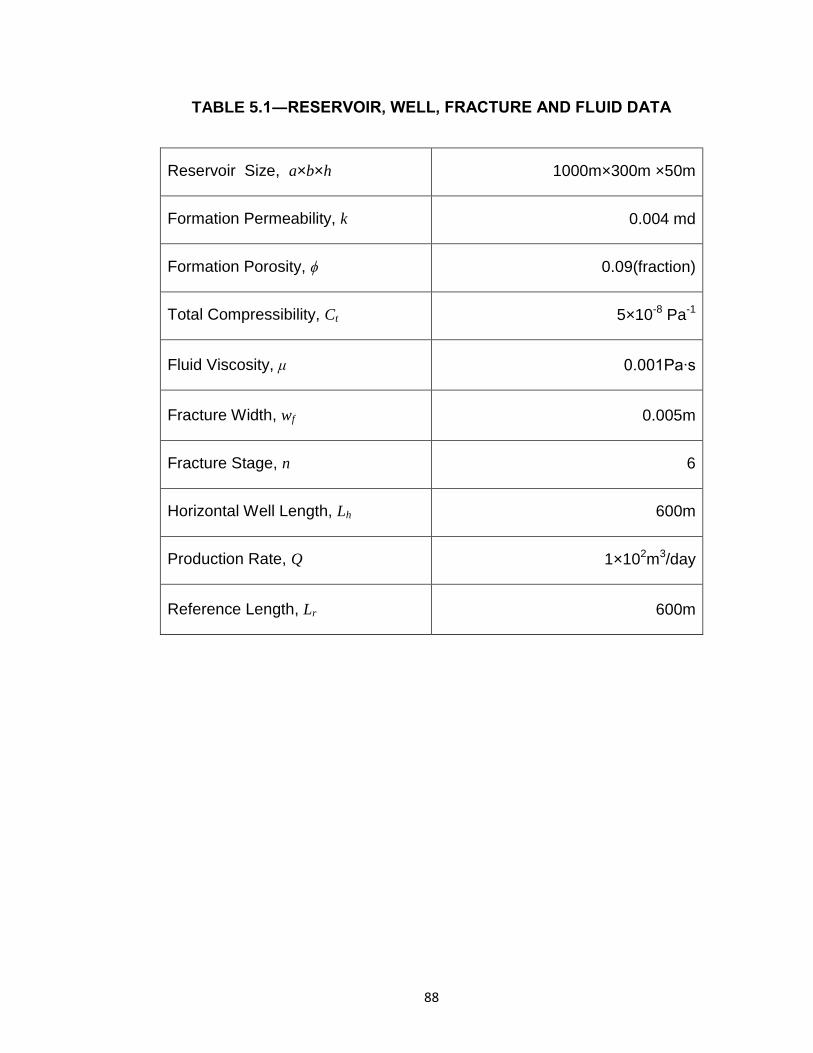
88
TABLE 5.1―RESERVOIR, WELL, FRACTURE AND FLUID DATA
Reservoir Size, a×b×h 1000m×300m ×50m
Formation Permeability, k 0.004 md
Formation Porosity, ϕ 0.09(fraction)
Total Compressibility, Ct 5×10⁻⁸ Pa-1
Fluid Viscosity, μ 0.001Pa∙s
Fracture Width, wf 0.005m
Fracture Stage, n 6
Horizontal Well Length, Lh 600m
Production Rate, Q 1×10²m3/day
Reference Length, Lr 600m

89
Figure 5.4―Transient pressure behaviour with stress-sensitive hydraulic
fractures.
tD
1e-6 1e-5 1e-4 1e-3 1e-2 1e-1 1e+0
Pw
D,
dP
wD
/dln
t D
0.001
0.01
0.1
1
10
CfDi
=50,df=2.5E-7 Pa
-1
CfDi
=50,df=0
Effective Pressure, MPa0 5 10 15 20 25
CfD
0
10
20
30
40
50
df=2.5E-7 Pa-1
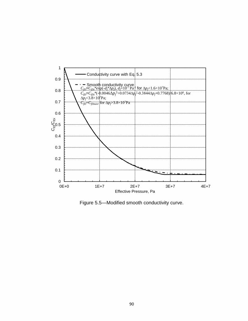
90
Figure 5.5―Modified smooth conductivity curve.
0
0.1
0.2
0.3
0.4
0.5
0.6
0.7
0.8
0.9
1
0E+0 1E+7 2E+7 3E+7 4E+7
CfD
/CfD
i
Effective Pressure, Pa
Conductivity curve with Eq. 5.3
Smooth conductivity curve CfD=CfDi*exp(-df*∆pf), df=10-7 Pa-1 for ∆pf<1.6×10⁷Pa;
CfD=CfDi*(-0.0046∆pf3+0.0734∆pf
2-0.3844∆pf+0.7768)/6.8×106, for
∆pf<3.8×10⁷Pa;
CfD=CfDmin, for ∆pf>3.8×10⁷Pa
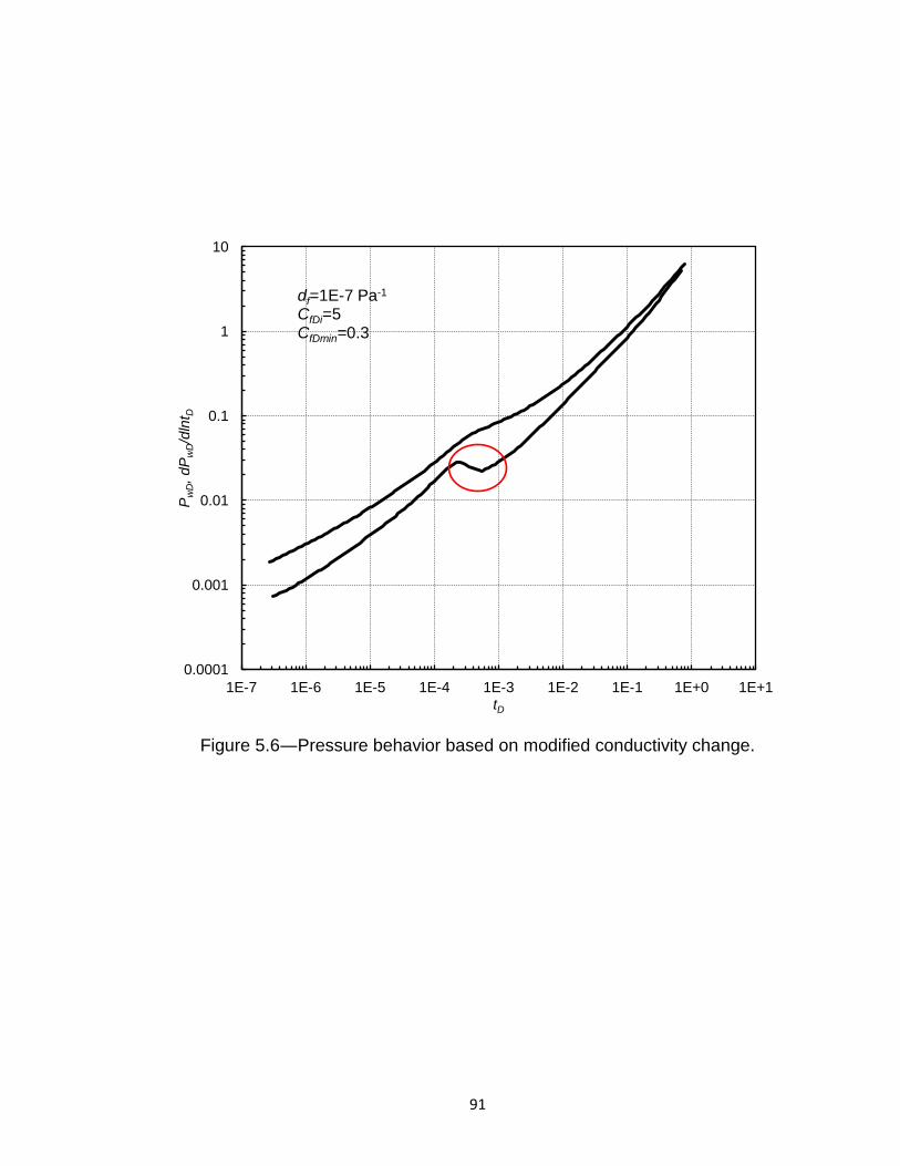
91
Figure 5.6―Pressure behavior based on modified conductivity change.
0.0001
0.001
0.01
0.1
1
10
1E-7 1E-6 1E-5 1E-4 1E-3 1E-2 1E-1 1E+0 1E+1
Pw
D, dP
wD/d
lnt D
tD
df=1E-7 Pa-1
CfDi=5 CfDmin=0.3
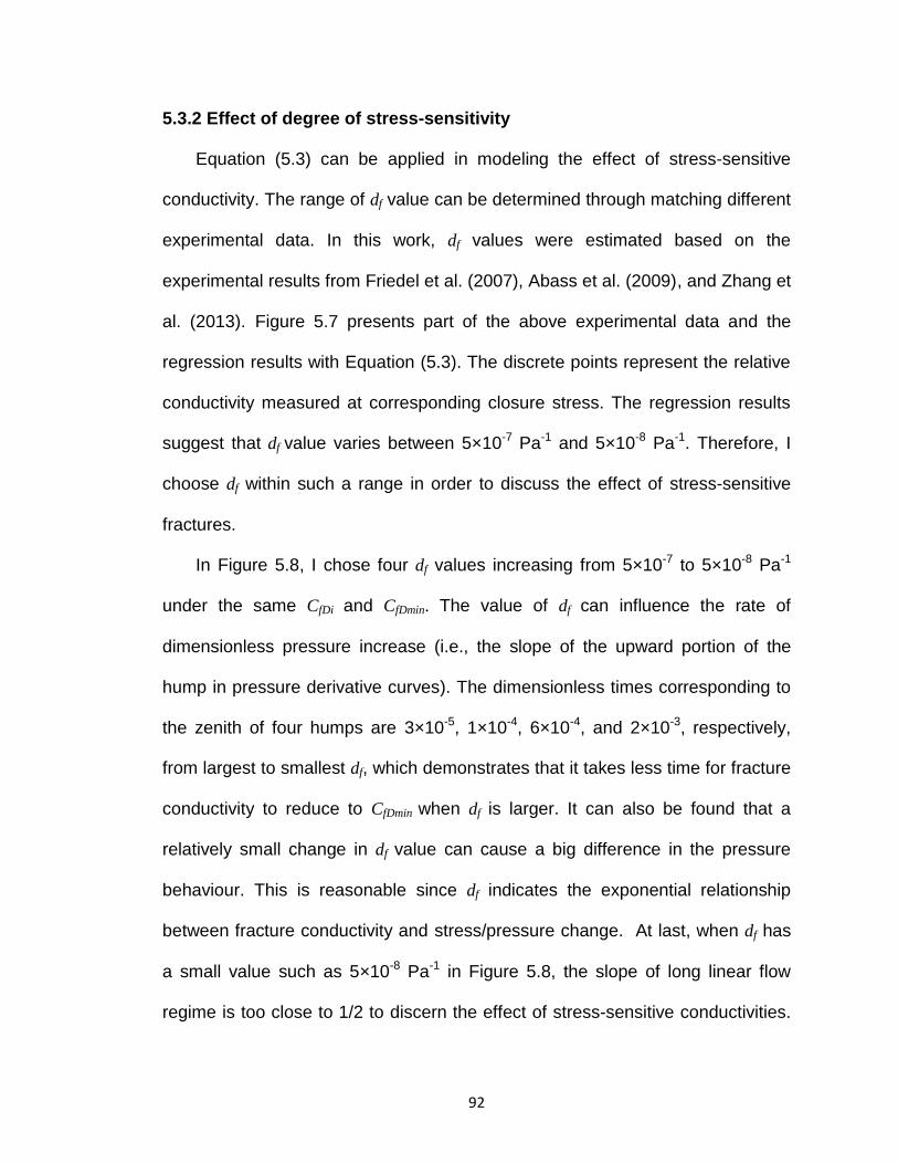
92
5.3.2 Effect of degree of stress-sensitivity
Equation (5.3) can be applied in modeling the effect of stress-sensitive
conductivity. The range of df value can be determined through matching different
experimental data. In this work, df values were estimated based on the
experimental results from Friedel et al. (2007), Abass et al. (2009), and Zhang et
al. (2013). Figure 5.7 presents part of the above experimental data and the
regression results with Equation (5.3). The discrete points represent the relative
conductivity measured at corresponding closure stress. The regression results
suggest that df value varies between 5×10⁻⁷ Pa-1 and 5×10⁻⁸ Pa-1. Therefore, I
choose df within such a range in order to discuss the effect of stress-sensitive
fractures.
In Figure 5.8, I chose four df values increasing from 5×10⁻⁷ to 5×10⁻⁸ Pa-1
under the same CfDi and CfDmin. The value of df can influence the rate of
dimensionless pressure increase (i.e., the slope of the upward portion of the
hump in pressure derivative curves). The dimensionless times corresponding to
the zenith of four humps are 3×10⁻⁵, 1×10⁻⁴, 6×10⁻⁴, and 2×10⁻³, respectively,
from largest to smallest df, which demonstrates that it takes less time for fracture
conductivity to reduce to CfDmin when df is larger. It can also be found that a
relatively small change in df value can cause a big difference in the pressure
behaviour. This is reasonable since df indicates the exponential relationship
between fracture conductivity and stress/pressure change. At last, when df has
a small value such as 5×10⁻⁸ Pa-1 in Figure 5.8, the slope of long linear flow
regime is too close to 1/2 to discern the effect of stress-sensitive conductivities.

93
On the whole, the pressure deviation will appear sooner and pressure derivative
slopes become larger with bigger df values and vice versa.
94
(Original in color)
Figure 5.7―Normalized fractures conductivities change with stress (Abass et al.,
2009 and Zhang, et al., 2013)
0.001
0.01
0.1
1
0 500 1000 1500 2000 2500 3000 3500 4000
CfD
/CfD
i
Closure stress, psi
df=5.5E-8, 9.5E-8, 1.1E-7,1.2E-7, 1.3E-7 and 2.6E-7 Pa-1
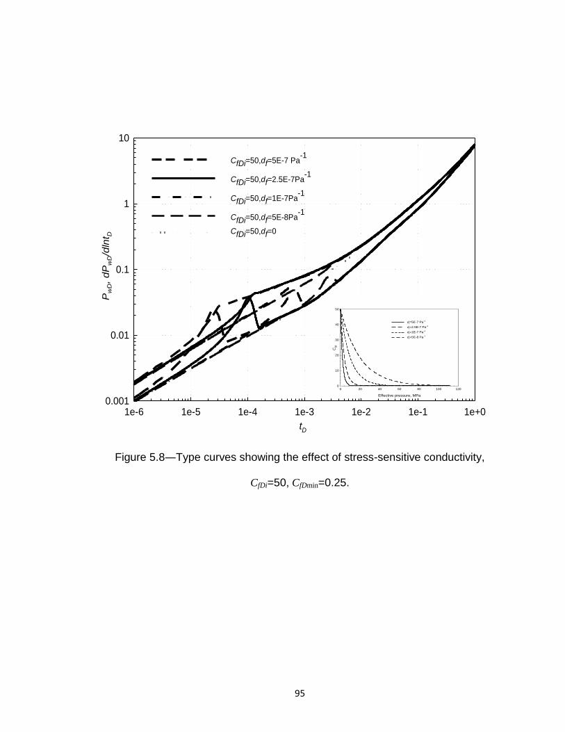
95
Figure 5.8―Type curves showing the effect of stress-sensitive conductivity,
CfDi=50, CfDmin=0.25.
tD
1e-6 1e-5 1e-4 1e-3 1e-2 1e-1 1e+0
Pw
D, dP
wD/d
lnt D
0.001
0.01
0.1
1
10
CfDi=50,df=5E-7 Pa-1
CfDi=50,df=2.5E-7Pa-1
CfDi=50,df=1E-7Pa-1
CfDi=50,df=5E-8Pa-1
CfDi=50,df=0
Effective pressure, MPa
0 20 40 60 80 100 120
CfD
0
10
20
30
40
50
df=5E-7 Pa-1
df=2.5E-7 Pa-1
df=1E-7 Pa-1
df=5E-8 Pa-1
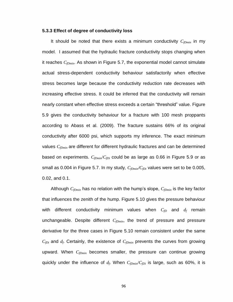
96
5.3.3 Effect of degree of conductivity loss
It should be noted that there exists a minimum conductivity CfDmin in my
model. I assumed that the hydraulic fracture conductivity stops changing when
it reaches CfDmin. As shown in Figure 5.7, the exponential model cannot simulate
actual stress-dependent conductivity behaviour satisfactorily when effective
stress becomes large because the conductivity reduction rate decreases with
increasing effective stress. It could be inferred that the conductivity will remain
nearly constant when effective stress exceeds a certain “threshold” value. Figure
5.9 gives the conductivity behaviour for a fracture with 100 mesh proppants
according to Abass et al. (2009). The fracture sustains 66% of its original
conductivity after 6000 psi, which supports my inference. The exact minimum
values CfDmin are different for different hydraulic fractures and can be determined
based on experiments. CfDmin/CfDi could be as large as 0.66 in Figure 5.9 or as
small as 0.004 in Figure 5.7. In my study, CfDmin/CfDi values were set to be 0.005,
0.02, and 0.1.
Although CfDmin has no relation with the hump’s slope, CfDmin is the key factor
that influences the zenith of the hump. Figure 5.10 gives the pressure behaviour
with different conductivity minimum values when CfD and df remain
unchangeable. Despite different CfDmin, the trend of pressure and pressure
derivative for the three cases in Figure 5.10 remain consistent under the same
CfDi and df. Certainly, the existence of CfDmin prevents the curves from growing
upward. When CfDmin becomes smaller, the pressure can continue growing
quickly under the influence of df. When CfDmin/CfDi is large, such as 60%, it is

97
possible that the hump disappears. When the fracture just loses a small part of
its conductivity, it is hard to discern the difference in the pressure behaviour with
and without stress-sensitive conductivity. In fact, such property is determined by
fracture characteristics. However, I can estimate the minimum conductivity value
through experiments in the laboratory. Generally, proppants with higher loading
strength have a larger CfDmin value, which can prevent serious fracture
conductivity reduction.
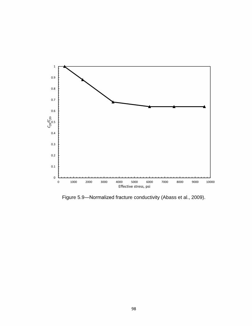
98
Figure 5.9―Normalized fracture conductivity (Abass et al., 2009).
0
0.1
0.2
0.3
0.4
0.5
0.6
0.7
0.8
0.9
1
0 1000 2000 3000 4000 5000 6000 7000 8000 9000 10000
CfD
/CfD
i
Effective stress, psi
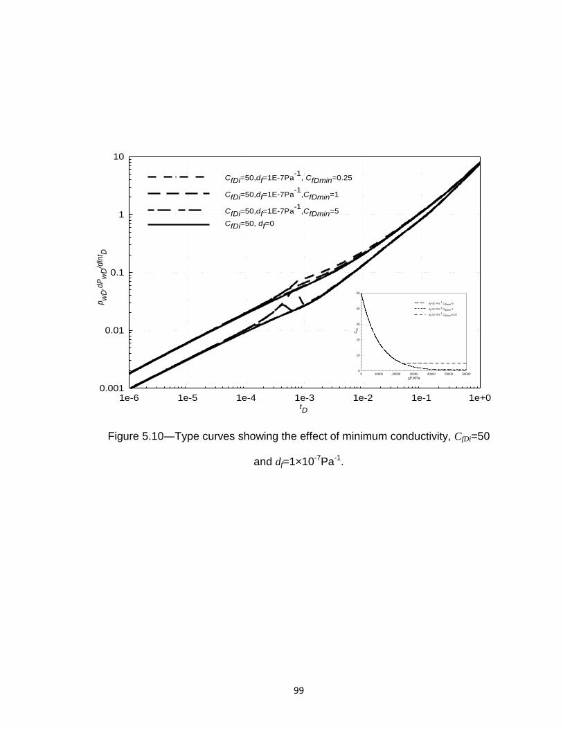
99
Figure 5.10―Type curves showing the effect of minimum conductivity, CfDi=50
and df=1×10⁻⁷Pa-1.
tD
1e-6 1e-5 1e-4 1e-3 1e-2 1e-1 1e+0
pw
D,d
Pw
D/d
lnt D
0.001
0.01
0.1
1
10
CfDi=50,df=1E-7Pa-1
, CfDmin=0.25
CfDi=50,df=1E-7Pa-1
,CfDmin=1
CfDi=50,df=1E-7Pa-1
,CfDmin=5
CfDi=50, df=0
P,KPa0 10000 20000 30000 40000 50000 60000
CfD
0
10
20
30
40
50
df=1E-7Pa-1
.CfDmin=5
df=1E-7Pa-1
.CfDmin=1
df=1E-7Pa-1
.CfDmin=0.25
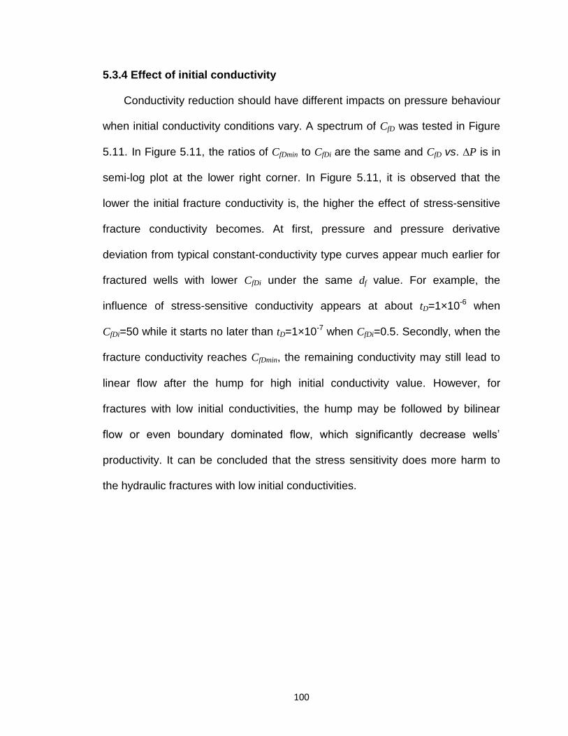
100
5.3.4 Effect of initial conductivity
Conductivity reduction should have different impacts on pressure behaviour
when initial conductivity conditions vary. A spectrum of CfD was tested in Figure
5.11. In Figure 5.11, the ratios of CfDmin to CfDi are the same and CfD vs. ∆P is in
semi-log plot at the lower right corner. In Figure 5.11, it is observed that the
lower the initial fracture conductivity is, the higher the effect of stress-sensitive
fracture conductivity becomes. At first, pressure and pressure derivative
deviation from typical constant-conductivity type curves appear much earlier for
fractured wells with lower CfDi under the same df value. For example, the
influence of stress-sensitive conductivity appears at about tD=1×10⁻⁶ when
CfDi=50 while it starts no later than tD=1×10⁻⁷ when CfDi=0.5. Secondly, when the
fracture conductivity reaches CfDmin, the remaining conductivity may still lead to
linear flow after the hump for high initial conductivity value. However, for
fractures with low initial conductivities, the hump may be followed by bilinear
flow or even boundary dominated flow, which significantly decrease wells’
productivity. It can be concluded that the stress sensitivity does more harm to
the hydraulic fractures with low initial conductivities.
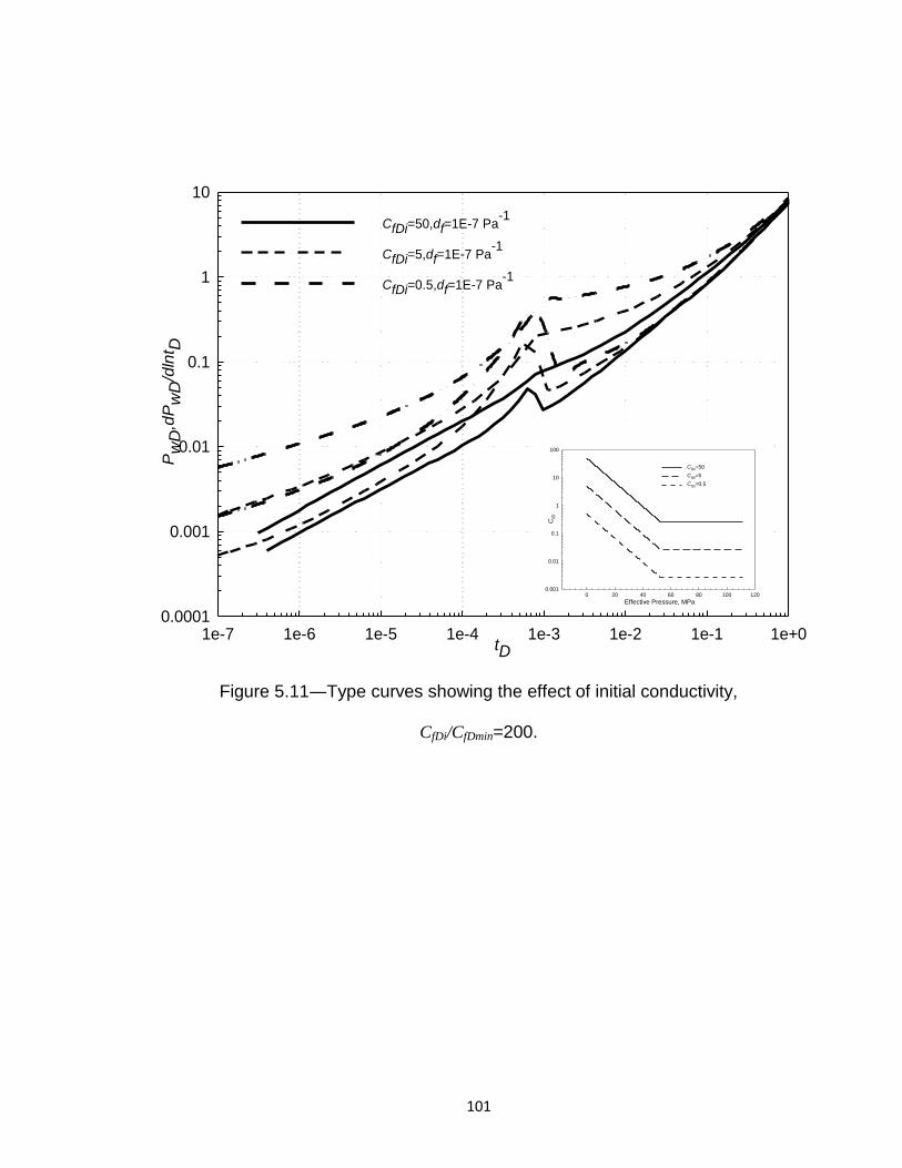
101
Figure 5.11―Type curves showing the effect of initial conductivity,
CfDi/CfDmin=200.
tD1e-7 1e-6 1e-5 1e-4 1e-3 1e-2 1e-1 1e+0
Pw
D,d
Pw
D/d
lnt D
0.0001
0.001
0.01
0.1
1
10
CfDi=50,df=1E-7 Pa-1
CfDi=5,df=1E-7 Pa-1
CfDi=0.5,df=1E-7 Pa-1
Effective Pressure, MPa0 20 40 60 80 100 120
CfD
0.001
0.01
0.1
1
10
100
CfDi=50
CfDi=5
CfDi=0.5
102
5.3.5 Stress-sensitive conductivity
In addition to the pressure behaviour, the relationship of the stress-sensitive
conductivity vs. time in production can also be represented. Figure 5.12 shows
the ratios of CfD to CfDi over time in semi-log plots for CfDi=50, CfDi=5 and CfDi=0.5
with different df. It is observed that higher df value reduces the fracture
conductivity more severely. For example, the fracture loses approximately 60%
of its conductivity in about 15 days when df equals 5×10⁻⁷ Pa-1. As discussed
before, the conductivity’s rapid reduction changes the slopes of bilinear/linear
flow regimes. Correspondingly, higher df makes the conductivity reduction
appear sooner and faster in Figure 5.12. I also compared the conductivities’
response when different initial conductivities were set in the model. It illustrates
that small stress-dependent characteristic values (df =1×10⁻⁷, and 5×10⁻⁸Pa-1)
have nearly the same effect on fractures with either high or low initial
conductivities. However, with high stress sensitivities (df =5×10⁻⁷, and 2.5×10-
7Pa-1), fracture conductivities with low initial values reduce more quickly than
those with high initial conductivity values.
Generally, the stress-sensitive effect on pressure behaviour of fractured
wells is mainly based on df, CfDmin and CfDi. Among these three factors, df has the
greatest impact on pressure behaviour. Higher df can make the pressure
increase more rapidly and the pressure derivate curve’s slope turns steeper.
The hump will appear sooner when df is large. The minimum conductivity CfDmin
determines the zenith of the hump. The fracture with low initial conductivity is
more susceptible to stress change during production.
103
Usually, the hump’s appearance could be determined by df, CfDmin and CfDi.
However, it is not usual to catch the complete hump in the field. As is discussed,
the hump is notable only when df is large and CfDmin is small. However, the well
would be shut-in for improvement if the fracture conductivity becomes too small
to produce economically. Therefore, it is difficult to see the downward part of the
hump. The upward part before the zenith in the hump is more common in many
wells with stress-sensitive hydraulic fractures whose slope is related with df and
CfDi.
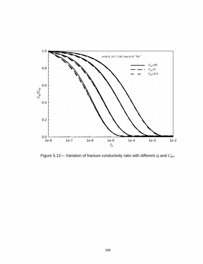
104
Fig.10― Variation of fracture conductivity ratio with different df and CfDi.
Figure 5.12― Variation of fracture conductivity ratio with different df and CfDi.
tD
1e-8 1e-7 1e-6 1e-5 1e-4 1e-3 1e-2
CfD
/CfD
i
0.0
0.2
0.4
0.6
0.8
1.0
CfDi
=50
CfDi
=5
CfDi
=0.5
df=5E-8, 1E-7, 2.5E-7and 5×10⁻⁷ Pa
-1
105
5.4 Field example
The field data were first used by Clarkson et al. (2012). The horizontal well
located in the Haynesville Shale is multi-stage fractured in 18 stages with eight
perforation clusters per stage spaced approximately 27 ft apart. Gas and water
production data for about 700 days were collected in a log-log scale plot in
Figure 5.13.
Clarkson et al. (2012) analyzed the production data in detail. They started
with assuming both constant matrix permeability and fracture conductivity. Then,
they considered dynamic matrix permeability only, which was followed by adding
stress-sensitive fracture conductivity into the analysis. Although the system
permeability and fracture half-length could be estimated in Clarkson et al.’s work,
no information about fracture conductivity reduction could be derived. Based on
the type curve matching by my model, however, it becomes easier to track
fracture properties. No other additional completion/reservoir details and well
locations were provided because of operator confidentiality. Therefore, in order
to evaluate the changing fracture conductivity, my transient pressure analysis is
directly based on results from Clarkson et al.
5.4.1 Analysis without corrections in matrix permeability
Figures 5.14a and 5.14b show the rate-normalized pseudopressure versus
time and rate-normalized pseudopressure derivatives versus time, respectively.
In Figures 5.14a and 5.14b, no corrections in the pseudopressure and time
function for dynamic matrix permeability are made by Clarkson et al. (2012). For
many fractured horizontal wells in shale formations, the linear flow may last for
106
several years. However, the linear flow in Figures 5.14b is very short, which is
followed by apparent BDF with pressure and its derivatives rising rapidly. This
phenomenon could be an obvious index for the decreasing fracture conductivity
and matrix permeability, which provides the basis for my analysis.
In my transient pressure analysis, assuming either one fracture per stage or
one fracture per cluster is acceptable. Here, I chose the horizontal well model
with 18 fractures instead of 144 fractures because of computation efficiency. In
accordance with Clarkson et al.’s results, I generated a series of type curves to
measure the fractures’ stress-dependent characteristic df. Figures 5.15a and
5.15b present the matching results. The matrix permeability used in my model is
based on Clarkson et al.’s results. The fracture conductivity reduces quickly from
1.34×10⁻¹³ m3 to 1.54×10⁻¹⁷ m3 with df =1.97×10⁻⁷ Pa-1 when matrix permeability
remains constant during 700 days of production.
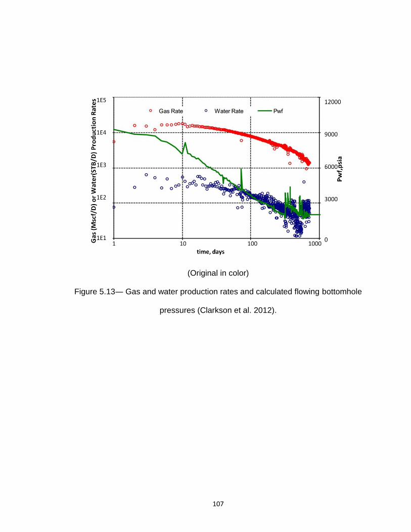
107
(Original in color)
Figure 5.13― Gas and water production rates and calculated flowing bottomhole
pressures (Clarkson et al. 2012).

108
(a)
(b)
Figure 5.14―Pressure and pressure derivative without corrections in matrix
permeability (Clarkson et al., 2012).
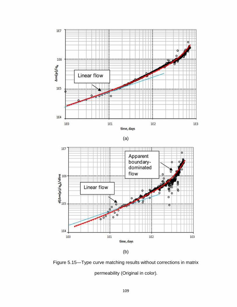
109
(a)
(b)
Figure 5.15―Type curve matching results without corrections in matrix
permeability (Original in color).
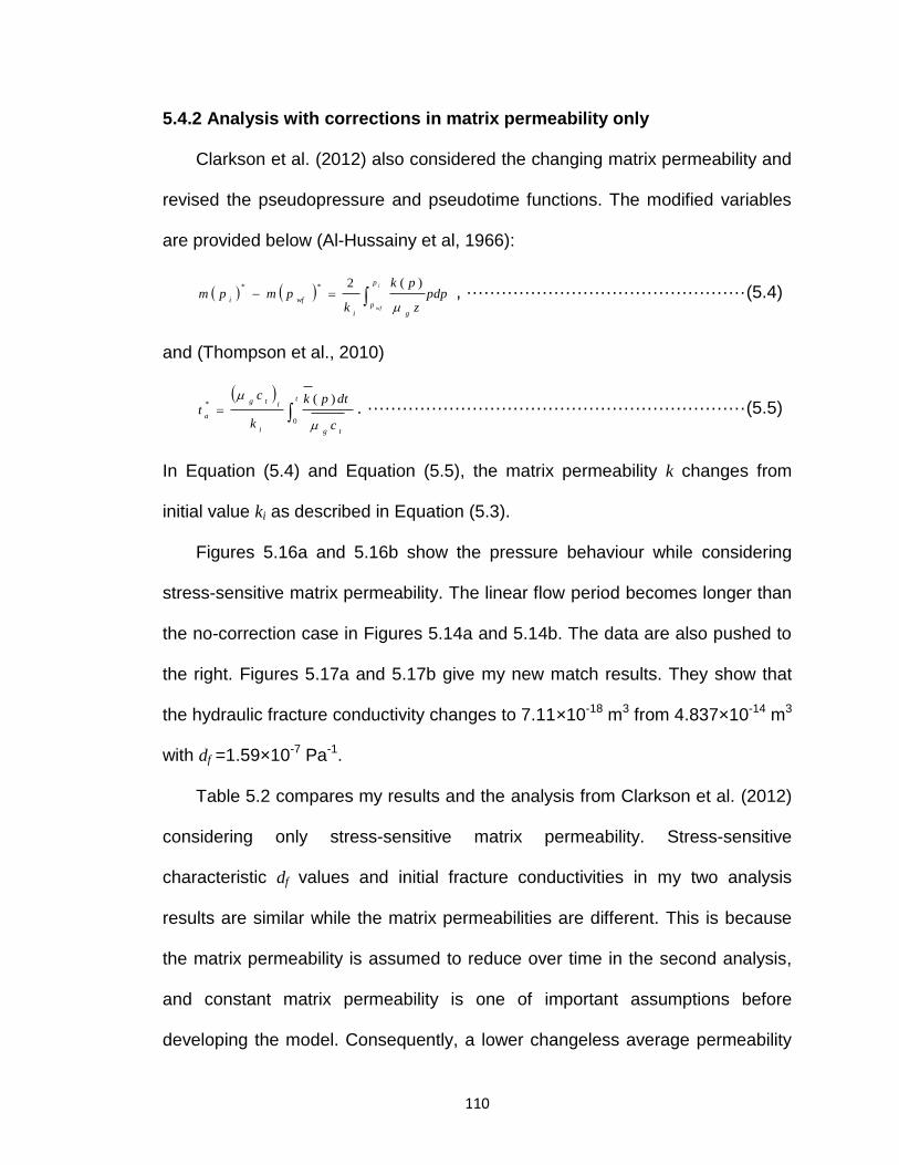
110
5.4.2 Analysis with corrections in matrix permeability only
Clarkson et al. (2012) also considered the changing matrix permeability and
revised the pseudopressure and pseudotime functions. The modified variables
are provided below (Al-Hussainy et al, 1966):
pdpz
pk
kpmpm
i
wf
p
pgi
wfi
)(2**
, ················································ (5.4)
and (Thompson et al., 2010)
t
tgi
itg
a
c
dtpk
k
c
t0
* )(
. ································································· (5.5)
In Equation (5.4) and Equation (5.5), the matrix permeability k changes from
initial value ki as described in Equation (5.3).
Figures 5.16a and 5.16b show the pressure behaviour while considering
stress-sensitive matrix permeability. The linear flow period becomes longer than
the no-correction case in Figures 5.14a and 5.14b. The data are also pushed to
the right. Figures 5.17a and 5.17b give my new match results. They show that
the hydraulic fracture conductivity changes to 7.11×10⁻¹⁸ m3 from 4.837×10⁻¹⁴ m3
with df =1.59×10⁻⁷ Pa-1.
Table 5.2 compares my results and the analysis from Clarkson et al. (2012)
considering only stress-sensitive matrix permeability. Stress-sensitive
characteristic df values and initial fracture conductivities in my two analysis
results are similar while the matrix permeabilities are different. This is because
the matrix permeability is assumed to reduce over time in the second analysis,
and constant matrix permeability is one of important assumptions before
developing the model. Consequently, a lower changeless average permeability

111
value is attained in my matching results to replace the stress-sensitive matrix
permeability.
Based on the analysis results with only stress-sensitive hydraulic fractures,
the forecast of production rate is provided. It is assumed that the bottomhole
pressure is constant at 2000 psi in the next 300 days. The prediction with both
stress-sensitive hydraulic fractures and matrix permeability are impracticable
because of lack of accurate pressure data. At the same time, the prediction
without stress-sensitivity from the aforementioned semi-analytical model is also
shown for comparison in Figure 5.18. The apparent BDF is regarded as real
BDF in the model with constant fracture properties. The result indicates that the
well’s productivity could be underestimated when the stress-sensitivity is
mistaken for the influence of boundaries.
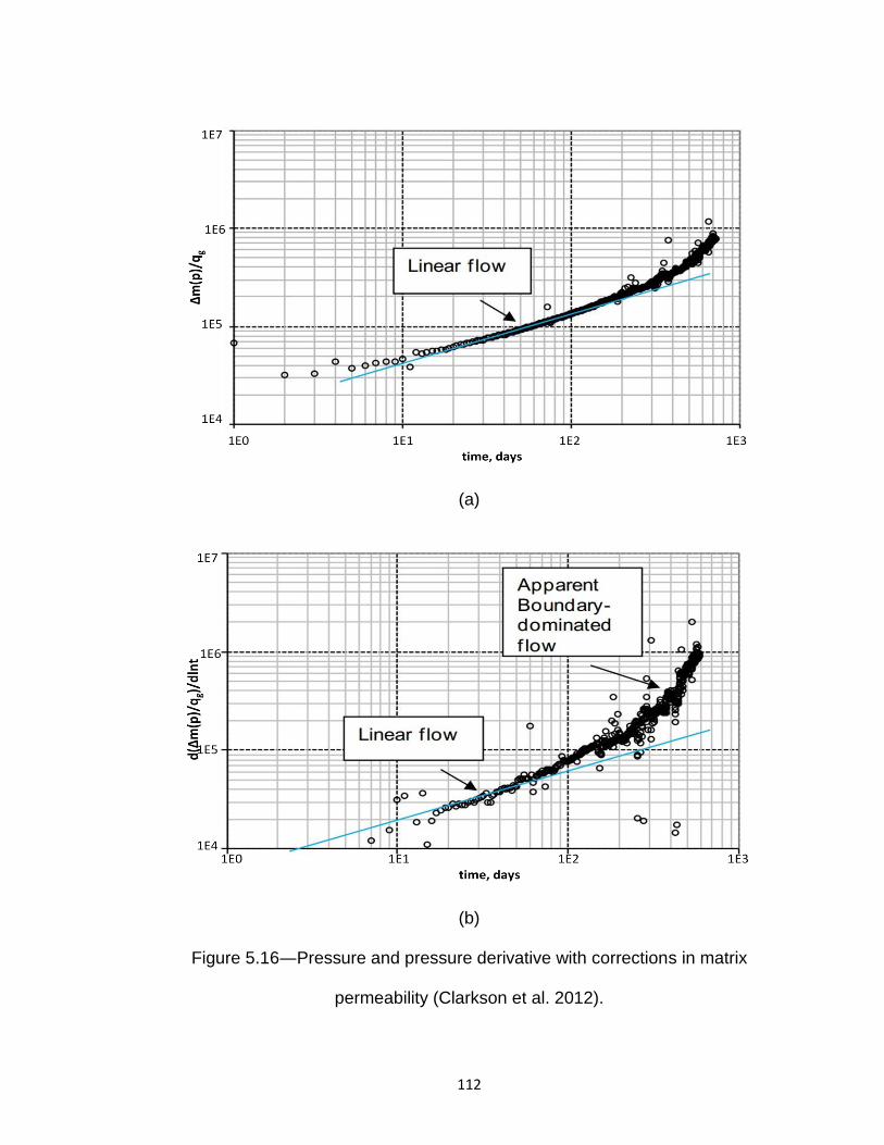
112
(a)
(b)
Figure 5.16―Pressure and pressure derivative with corrections in matrix
permeability (Clarkson et al. 2012).
113
(a)
(b)
Figure 5.17―Type curve matching results with corrections in matrix
permeability (Original in color).
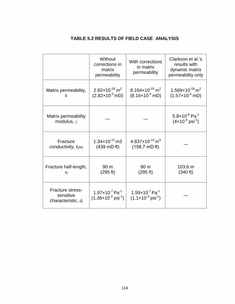
114
TABLE 5.2 RESULTS OF FIELD CASE ANALYSIS
Without
corrections in matrix
permeability
With corrections in matrix
permeability
Clarkson et al.’s results with
dynamic matrix permeability only
Matrix permeability, k
2.82×10⁻¹⁸ m2 (2.82×10⁻³ mD)
8.164×10⁻¹⁹ m2
(8.16×10⁻⁴ mD) 1.569×10⁻¹⁸ m2 (1.57×10⁻³ mD)
Matrix permeability modulus, γ
― ― 5.8×10⁻⁸ Pa-1 (4×10⁻⁴ psi-1)
Fracture conductivity, kfwf
1.34×10⁻¹³ m3 (439 mD∙ft)
4.837×10⁻¹⁴ m3 (158.7 mD∙ft)
―
Fracture half-length, xf
90 m (295 ft)
90 m (295 ft)
103.6 m (340 ft)
Fracture stress-sensitive
characteristic, df
1.97×10⁻⁷ Pa-1 (1.36×10⁻³ psi-1)
1.59×10⁻⁷ Pa-1 (1.1×10⁻³ psi-1)
―
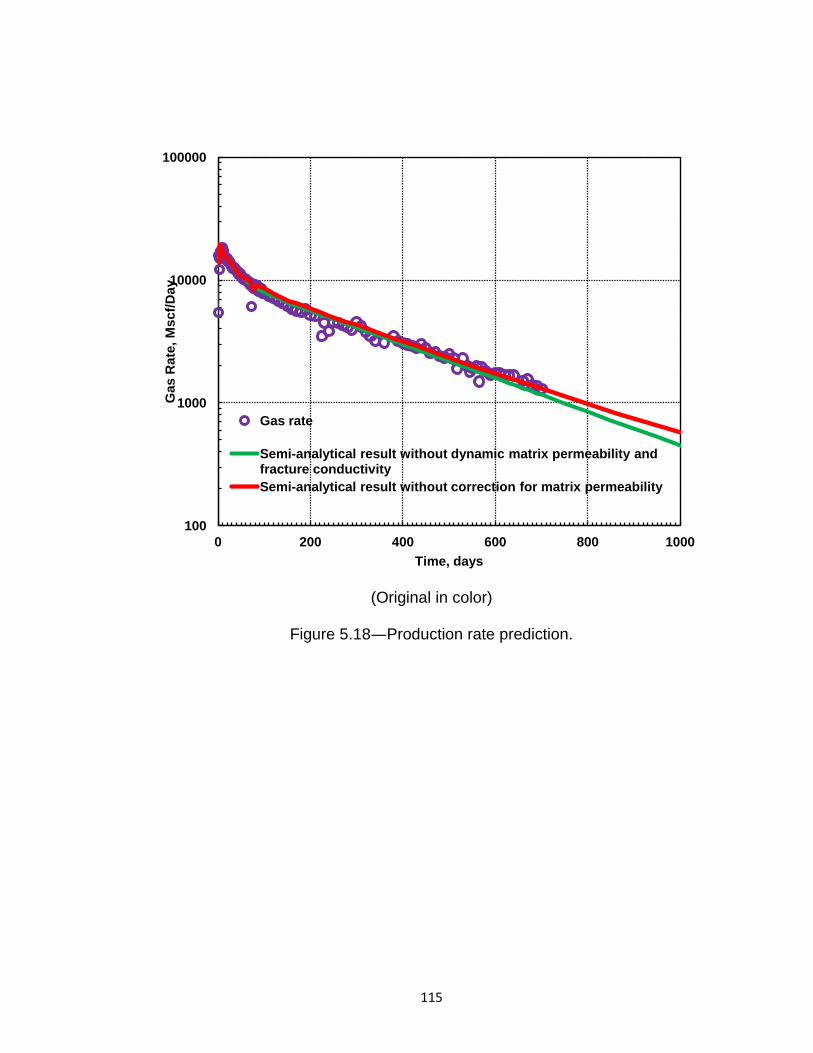
115
(Original in color)
Figure 5.18―Production rate prediction.
100
1000
10000
100000
0 200 400 600 800 1000
Gas R
ate
, M
scf/
Day
Time, days
Gas rate
Semi-analytical result without dynamic matrix permeability and fracture conductivity
Semi-analytical result without correction for matrix permeability
116
5.5 Chapter summary
The study of stress-sensitive hydraulic fractures is crucial for optimizing and
monitoring fracturing treatments, especially for unconventional reservoirs. In this
chapter, I modeled and discussed the pressure behaviour of wells with stress-
dependent hydraulic fractures. Based on my work, several conclusions can be
drawn:
A semi-analytical model has been established and type curves are
generated based on the model for pressure transient analysis of fractured
wells.
When the stress-sensitive fracture conductivity reduces, the slopes of
bilinear/linear flow become larger than 1/4 and 1/2, respectively. A hump
can be formed in the pressure derivative curve, and its slope is close to or
even larger than unit.
Large df could make the pressure derivative curve slopes increase
quickly and accelerate the hump’s appearance. The minimum
conductivity CfDmin can stop the conductivity from decreasing to a very
small value in this model.
The pressure deviation from that with constant fracture conductivities is
influenced by initial fracture conductivities. The lower the initial fracture
conductivity, the greater the effect of stress-sensitive conductivity.
When df value is small, it has a similar influence on the conductivity ratio
no matter whether the fracture has a high or low initial conductivity. When
117
df becomes larger, the fractures with low initial conductivities lose their
conductivities more quickly.
The applicability of this semi-analytical model is proved in the field case
study based on an example from the literature. It shows that incorrect
conclusions could be drawn if the stress-sensitive effect of hydraulic
fractures is ignored.
118
CHAPTER 6
PRODUCTION RATE ANALYSIS
Production rate analysis has been widely used by petroleum engineers to
evaluate reservoir performance and predict wells’ production. For multi-stage
fractured horizontal wells, the production rate analysis in this chapter also
considers the stress-sensitive hydraulic fracture conductivity. Traditional
analytical methods might cause errors in predicting wells’ performance under
complex well/reservoir conditions. Therefore, in addition to analytical solutions,
this work provides accurate semi-analytical modeling for multi-stage fractured
horizontal wells with constant bottomhole pressure.
At first, a few assumptions, listed below, should be made, as in Chapter 5:
1. The target formation is isotropic, homogeneous, and bounded with upper
and lower impermeable strata. All the boundaries are closed boundaries.
2. Reservoir parameters, such as porosity ϕ and permeability k are kept
constant during production.
3. Both the reservoir and hydraulic fractures are filled with single-phase
fluid, which could be gas or slightly compressible fluid with constant viscosity.
4. All the hydraulic fractures are vertical, symmetric, and fully penetrate
the formation.
119
6.1 Model and algorithm
The mathematical model for multi-stage fractured horizontal wells under
constant-pressure condition is similar to that with constant production rate. The
fluid flow from reservoir to wellbore is negligible. Dimensionless definitions of
variables are the same as in section 4.1. Since the production rate changes over
time in constant-pressure production, a reference oil production rate Qr is
necessary in dimensionless definition:
r
wfi
D
Q
ppkhp
)( , ········································································· (6.1)
r
rrf
rfD
Q
Lqq , ············································································· (6.2)
r
f
fD
Q
qq . ················································································· (6.3)
For gas wells, I also have (Al-Hussainy et al., 1966)
scr
wfisc
DTpQ
pmpmkhTp
))()(( , ······························································· (6.4)
where Tsc and psc are the standard temperature and pressure, respectively.
The reference rate Qr can be any value but remains consistent throughout
the whole model. In the following discussion, the reference rate Qr is 105 m3/day.
The whole system is still seperated into two parts: one is the fluid flow system
inside the hydraulic fractures and the other is the fluid flow system inside the
reservoir. Each hydraulic fracture is divided into several segments, and each
segment owns a uniform influx from the reservoir systemqrfi,j and two node
fluxes from adjacent fracture segments inside fractures qrfi,j-1 andqrfi,j. At the
120
end of every time step, the segment solutions for the reservoir system that are in
a linear format with jrfi
q,
are coupled with fracture segment solutions by using
the pressure equivalent and flux continuity conditions at the interfaces of any
two adjacent segments at the same time point in Laplace domain. In addition,
the pressure of fracture segments closest to the wellbore should be equal to the
constant flowing bottomhole pressure. Finally, fluxes at each interface and
pressure distribution in the reservoir can be achieved.
For fractured wells with stress-sensitive hydraulic fractures, the algorithm is
presented in Chapter 3 and Chapter 5. Fracture conductivities change as
described by Equation (5.3). The difference of this constant-pressure model with
dynamic conductivities when compared with the constant-rate stress-sensitive
model is that here the initial pressure is chosen to be the pressure distribution
when fractured wells start to produce rather than Pi.
6.2 Model validation
This study presents a rigorous semi-analytical model for a 6-stage fractured
horizontal well located in the center of a rectangular closed reservoir. The model
was validated with the numerical case from KAPPA Ecrin. Figure 6.1 shows the
comparison between these two cases and a satisfactory match is reached. I
preferred the numerical model to the analytical model in KAPPA Ecrin because
the data from the analytical KAPPA model become unstable in the BDF regime.
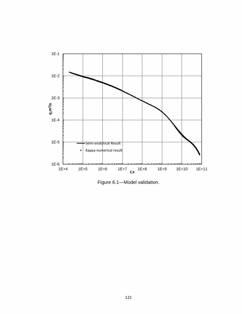
121
Figure 6.1―Model validation.
1E-6
1E-5
1E-4
1E-3
1E-2
1E-1
1E+4 1E+5 1E+6 1E+7 1E+8 1E+9 1E+10 1E+11
q,m
3/s
t,s
Semi-analytical Result
Kappa numerical result
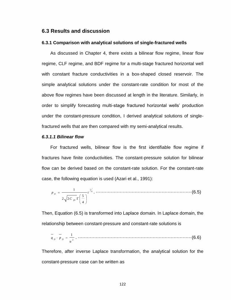
122
6.3 Results and discussion
6.3.1 Comparison with analytical solutions of single-fractured wells
As discussed in Chapter 4, there exists a bilinear flow regime, linear flow
regime, CLF regime, and BDF regime for a multi-stage fractured horizontal well
with constant fracture conductivities in a box-shaped closed reservoir. The
simple analytical solutions under the constant-rate condition for most of the
above flow regimes have been discussed at length in the literature. Similarly, in
order to simplify forecasting multi-stage fractured horizontal wells’ production
under the constant-pressure condition, I derived analytical solutions of single-
fractured wells that are then compared with my semi-analytical results.
6.3.1.1 Bilinear flow
For fractured wells, bilinear flow is the first identifiable flow regime if
fractures have finite conductivities. The constant-pressure solution for bilinear
flow can be derived based on the constant-rate solution. For the constant-rate
case, the following equation is used (Azari et al., 1991):
41
4
522
1t
C
p
fD
D
. ································································ (6.5)
Then, Equation (6.5) is transformed into Laplace domain. In Laplace domain, the
relationship between constant-pressure and constant-rate solutions is
2
1
upq
DD . ············································································ (6.6)
Therefore, after inverse Laplace transformation, the analytical solution for the
constant-pressure case can be written as
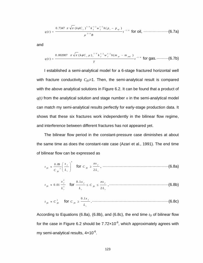
123
4/1
4/3
2/12/14/1)()(7347.0
)(
tB
pphwkCk
tqwfifft
for oil, ··················· (6.7a)
and
4/1
2/12/14/1
)()(002007.0
)(
tT
mmhwkCk
tqpwfpiffit
for gas. ········· (6.7b)
I established a semi-analytical model for a 6-stage fractured horizontal well
with fracture conductivity CfD=1. Then, the semi-analytical result is compared
with the above analytical solutions in Figure 6.2. It can be found that a product of
q(t) from the analytical solution and stage number n in the semi-analytical model
can match my semi-analytical results perfectly for early-stage production data. It
shows that these six fractures work independently in the bilinear flow regime,
and interference between different fractures has not appeared yet.
The bilinear flow period in the constant-pressure case diminishes at about
the same time as does the constant-rate case (Azari et al., 1991). The end time
of bilinear flow can be expressed as
4
2
09.0
r
f
fD
fD
L
x
C
t for r
f
fD
L
xC
2
, ·················································· (6.8a)
2
2
01.0
r
f
fD
L
xt for
r
f
fD
r
f
L
xC
L
x
2
1.0 , ············································· (6.8b)
2
fDfDCt for
r
f
fD
L
xC
1.0 . ·························································· (6.8c)
According to Equations (6.8a), (6.8b), and (6.8c), the end time tD of bilinear flow
for the case in Figure 6.2 should be 7.72×10⁻⁶, which approximately agrees with
my semi-analytical results, 4×10⁻⁶.

124
Figure 6.2―Results comparison for bilinear flow.
1E-6
1E-5
1E-4
1E-3
1E-2
1E-1
1E-8 1E-7 1E-6 1E-5 1E-4 1E-3 1E-2 1E-1 1E+0
qD
tD
Semi-analytical results
Analytical solution for bilinear flow
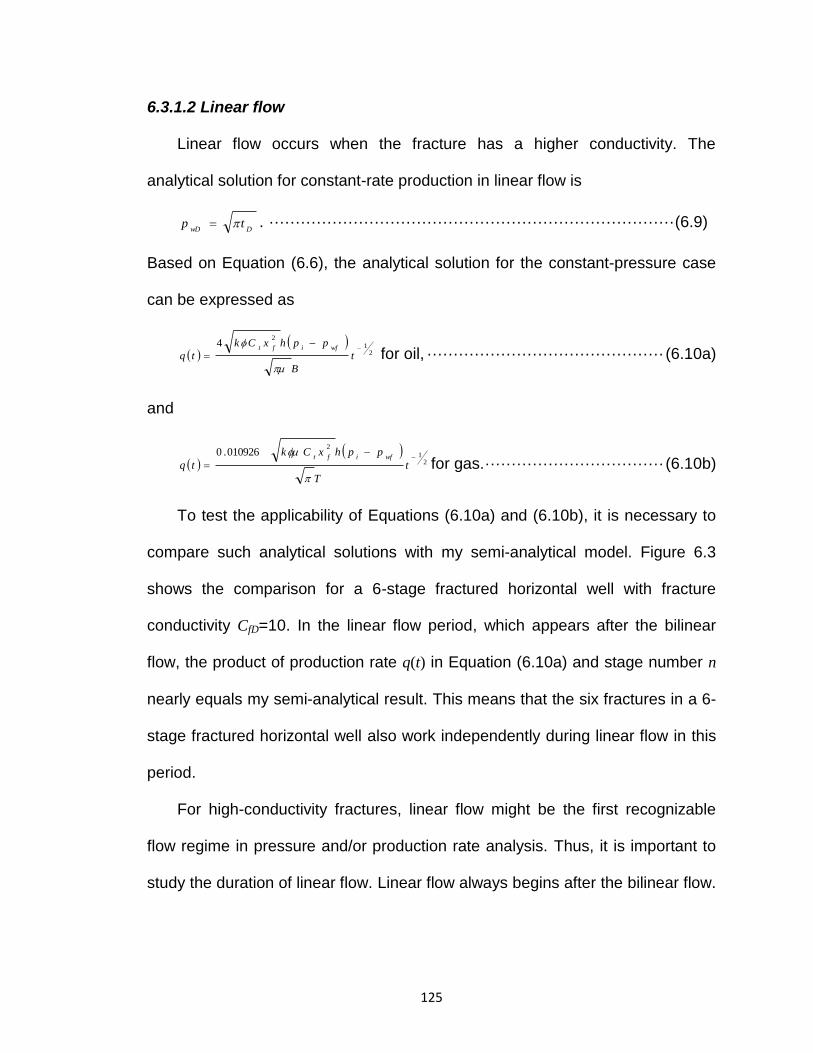
125
6.3.1.2 Linear flow
Linear flow occurs when the fracture has a higher conductivity. The
analytical solution for constant-rate production in linear flow is
DwDtp . ············································································· (6.9)
Based on Equation (6.6), the analytical solution for the constant-pressure case
can be expressed as
21
24
t
B
pphxCk
tqwfift
for oil, ············································· (6.10a)
and
21
2010926.0
t
T
pphxCk
tqwfift
for gas. ·································· (6.10b)
To test the applicability of Equations (6.10a) and (6.10b), it is necessary to
compare such analytical solutions with my semi-analytical model. Figure 6.3
shows the comparison for a 6-stage fractured horizontal well with fracture
conductivity CfD=10. In the linear flow period, which appears after the bilinear
flow, the product of production rate q(t) in Equation (6.10a) and stage number n
nearly equals my semi-analytical result. This means that the six fractures in a 6-
stage fractured horizontal well also work independently during linear flow in this
period.
For high-conductivity fractures, linear flow might be the first recognizable
flow regime in pressure and/or production rate analysis. Thus, it is important to
study the duration of linear flow. Linear flow always begins after the bilinear flow.
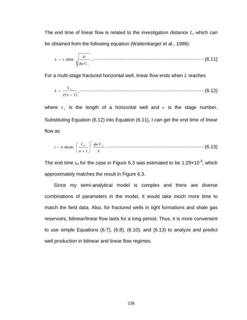
126
The end time of linear flow is related to the investigation distance L, which can
be obtained from the following equation (Wattenbarger et al., 1998):
tC
ktL
9856.1 . ······································································ (6.11)
For a multi-stage fractured horizontal well, linear flow ends when L reaches
12
n
LL
h , ·············································································· (6.12)
where hL is the length of a horizontal well and n is the stage number.
Substituting Equation (6.12) into Equation (6.11), I can get the end time of linear
flow as
k
C
n
Lt
th
2
106341.0
. ····························································· (6.13)
The end time tD for the case in Figure 6.3 was estimated to be 1.29×10⁻³, which
approximately matches the result in Figure 6.3.
Since my semi-analytical model is complex and there are diverse
combinations of parameters in the model, it would take much more time to
match the field data. Also, for fractured wells in tight formations and shale gas
reservoirs, bilinear/linear flow lasts for a long period. Thus, it is more convenient
to use simple Equations (6.7), (6.8), (6.10), and (6.13) to analyze and predict
well production in bilinear and linear flow regimes.
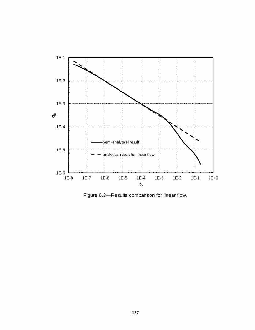
127
Figure 6.3―Results comparison for linear flow.
1E-6
1E-5
1E-4
1E-3
1E-2
1E-1
1E-8 1E-7 1E-6 1E-5 1E-4 1E-3 1E-2 1E-1 1E+0
qD
tD
Semi-analytical result
analytical result for linear flow

128
6.3.1.3 Compound linear flow
Compound linear flow is similar to the aforementioned linear flow with one
half slope in production rate curves in the log-log plot. However, the difference
for compound linear flow is that the flow during this period is perpendicular to the
direction of linear flow.
Figure 6.4 shows the production rates for 6-stage fractured horizontal wells
with different fracture half-lengths among which only the well with fracture half-
length xf=40m exhibits the compound formation linear flow clearly. It can be
concluded that the appearance of a compound linear flow regime depends upon
the fractures’ half-length xf . This conclusion agrees with Chen and Raghavan’s
(1997) results. When xf=40 m and ye (inter-well spacing) =400 m, the ratio of xf
vs. ye is 0.1, which indicates that ye must be at least 10 times greater than xf if
the compound linear flow is obvious. Accordingly, it is very unlikely for the
compound linear flow to appear in field applications and, therefore, any
departure from the linear flow in production rate analysis should not be
interpreted as compound linear flow without verification.
Similar to Equation (6.10), the analytical solution for compound linear flow
under the constant-pressure condition is
21
22
t
B
pphxCktq
wfict
for oil, ········································· (6.14a)
and
21
2010926.0
t
T
pphxCktq
wfict
for gas. ····························· (6.14b)
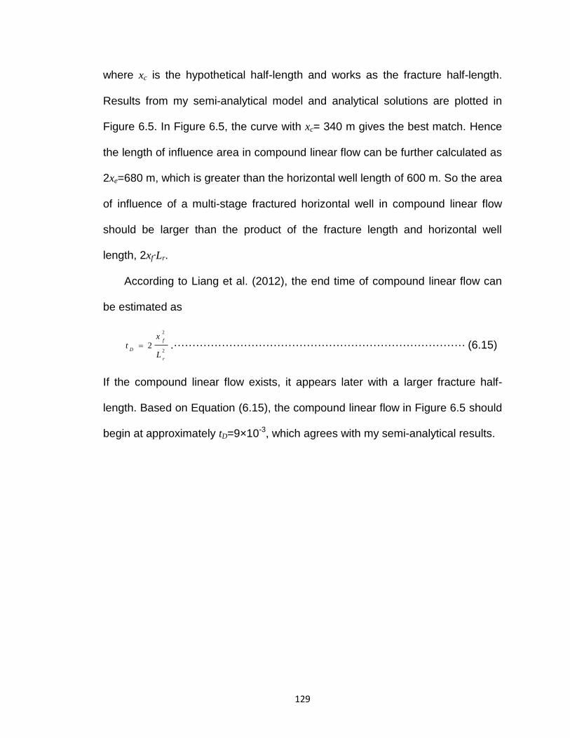
129
where xc is the hypothetical half-length and works as the fracture half-length.
Results from my semi-analytical model and analytical solutions are plotted in
Figure 6.5. In Figure 6.5, the curve with xc= 340 m gives the best match. Hence
the length of influence area in compound linear flow can be further calculated as
2xe=680 m, which is greater than the horizontal well length of 600 m. So the area
of influence of a multi-stage fractured horizontal well in compound linear flow
should be larger than the product of the fracture length and horizontal well
length, 2xf∙Lr.
According to Liang et al. (2012), the end time of compound linear flow can
be estimated as
2
2
2
r
f
D
L
xt .··············································································· (6.15)
If the compound linear flow exists, it appears later with a larger fracture half-
length. Based on Equation (6.15), the compound linear flow in Figure 6.5 should
begin at approximately tD=9×10⁻³, which agrees with my semi-analytical results.
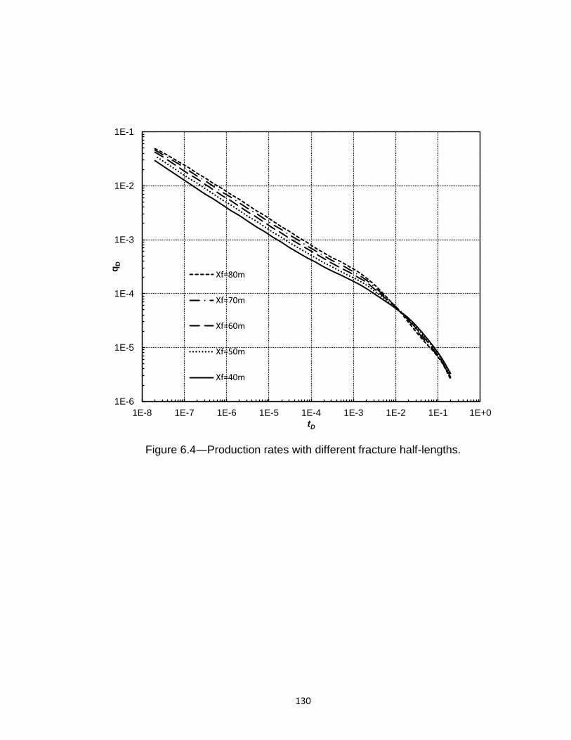
130
Figure 6.4―Production rates with different fracture half-lengths.
1E-6
1E-5
1E-4
1E-3
1E-2
1E-1
1E-8 1E-7 1E-6 1E-5 1E-4 1E-3 1E-2 1E-1 1E+0
qD
tD
Xf=80m
Xf=70m
Xf=60m
Xf=50m
Xf=40m
131
Figure 6.5―Results comparison for compound linear flow.
1E-6
1E-5
1E-4
1E-3
1E-2
1E-1
1E-8 1E-7 1E-6 1E-5 1E-4 1E-3 1E-2 1E-1 1E+0
qD
tD
Xf=40m,semi-analytical model result
Compound Formation Linear Flow, analytical result
132
6.3.1.4 Boundary-dominated flow
The onset of boundary dominated flow means that the area of influence of a
fractured horizontal well has reached the boundaries. The characteristic of
boundary dominated flow under the constant-rate condition is the unit slope of
both pressure and pressure derivative curves in a log-log plot. However, for
constant-pressure production, the slope of the production rate curve in the log-
log plot is no longer unit. Similar to sections 6.3.1.1 and 6.3.1.2, the analytical
constant-pressure solution for the boundary dominated flow can also be derived
from the analytical constant-rate solution. For a constant-rate production well,
the dimensionless pressure in BDF can be expressed as
batpDD . ·········································································· (6.16)
where a and b are the slope and intercept in a Cartesian coordinate system.
Following the steps in section 6.3.1.1, the dimensionless production rate under
constant flowing pressure should be
Dt
b
a
De
bq
1
. ··········································································· (6.17)
Equation (6.17) is a general exponential decline equation rather than a unit
slope equation. Figure 6.6 compares the analytical exponential solution
(a=5.4956×10⁴ and b=4.833×10⁵) with my semi-analytical result and BDF
exhibits an exponential trend as Eq. (6.17).
As discussed in Chapter 4, a pseudo pseudo-steady state flow regime is
very similar to boundary dominated flow under constant-rate condition, but in
constant-pressure solutions, pseudo pseudo-steady state flow also has a close-

133
to-unit slope, rather than exponential decline, so it can be further concluded that
the slope of pseudo pseudo-steady state flow under constant-rate condition is
not exactly unit or changes over time.
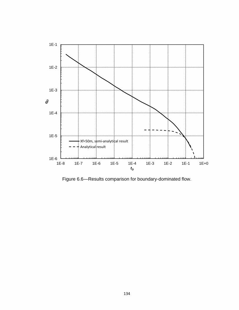
134
Figure 6.6―Results comparison for boundary-dominated flow.
1E-6
1E-5
1E-4
1E-3
1E-2
1E-1
1E-8 1E-7 1E-6 1E-5 1E-4 1E-3 1E-2 1E-1 1E+0
qD
tD
Xf=50m, semi-analytical result
Analytical result
135
6.3.2 Effect of stress-sensitive fracture conductivity
The effect of stress-sensitive fracture conductivities under constant-rate
condition has already been discussed in Chapter 5. In Chapter 6, I further
analyze such influence with the constant-pressure condition. Variables such as
df and CfD are investigated in detail through my semi-analytical model.
6.3.2.1 Effect of df
The df value demonstrates the hydraulic fractures’ stress-sensitive
characteristic. As suggested in section 5.3.2, the range of df was chosen to be
between 5×10⁻⁸ Pa-1and 3×10⁻⁷ Pa-1 in this study. Figure 6.7 provides the
production rate of a 6-stage fractured horizontal well with different stress-
sensitive fracture characteristics. The fracture conductivity reduces from initial
value CfDi=1 as described in Equation (5.3). The slopes of bilinear and linear
flows with stress-sensitive conductivities are exactly between 1/4 and 1/2 (1/4
<slope<1/2), which deviate from typical 1/4 and 1/2 slopes. Such slope
characteristic can be regarded as a sign of stress-sensitive fracture
conductivities. The larger df becomes, the bigger the slope deviation of bilinear
and linear flow will be. While bilinear and linear flows are influenced by stress-
dependent characteristic, the pseudo PSS flow and BDF are not affected by
such dynamic conductivities when df is relatively small.
The fracture conductivities vs. time are plotted in semi-log scale in Figure
6.8. Originally, fracture conductivities drop quickly over time. The slopes of
conductivity curves become greater if df becomes larger. However, the
136
conductivity tends to stop changing and approaches a minimum value C*
fDmin
after a period of reduction. Such minimum value is dependent on df, *
ip and pwf :
wfif ppd
fDifDeCC
*
*
min, ····························································· (6.18)
where the initial pressure *
ip is the pressure calculated at the first time step in
production and is related to xf and CfDi.

137
Figure 6.7― Production curves with different df.
1E-6
1E-5
1E-4
1E-3
1E-2
1E-1
1E-8 1E-7 1E-6 1E-5 1E-4 1E-3 1E-2 1E-1 1E+0
qD
tD
CfDi=3,df=0
CfDi=3,df=5E-8 Pa-1
CfDi=3,df=7E-8 Pa-1
CfDi=3,df=9E-8 Pa-1
CfDi=3,df=1E-7 Pa-1
CfDi=3,df=3E-7 Pa-1
xf=80m CfDi=1, df=0
CfDi=1, df=3E-7 Pa-1
CfDi=1, df=1E-7 Pa-1
CfDi=1, df=9E-8 Pa-1
CfDi=1, df=7E-8 Pa-1
CfDi=1, df=5E-8 Pa-1

138
Figure 6.8 ― Conductivity curves with different df .
0.0
0.1
0.2
0.3
0.4
0.5
0.6
0.7
0.8
0.9
1.0
1E-8 1E-7 1E-6 1E-5 1E-4 1E-3 1E-2 1E-1 1E+0
CfD
/CfD
i
tD
df=5E-8 Pa-1
df=7E-8 Pa-1
df=9E-8 Pa-1
df=1E-7 Pa-1
df=3E-7 Pa-1
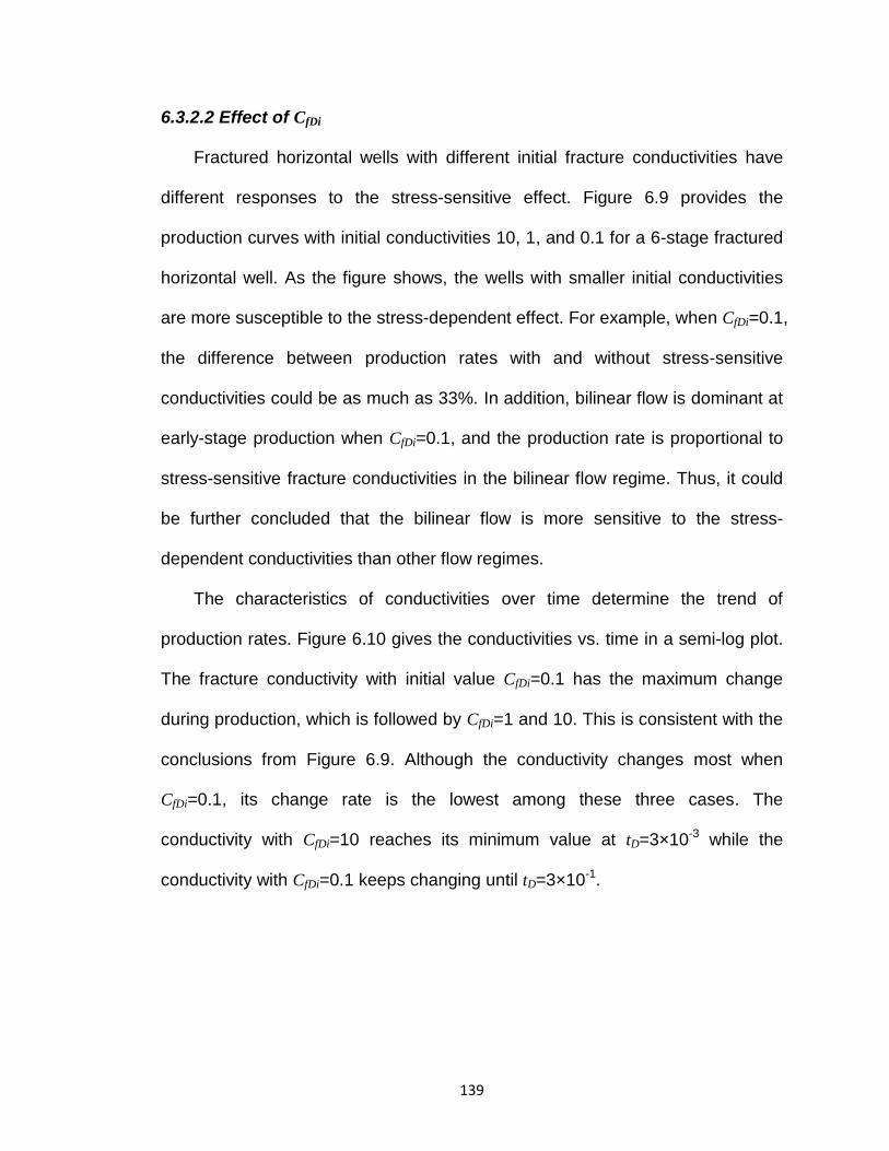
139
6.3.2.2 Effect of CfDi
Fractured horizontal wells with different initial fracture conductivities have
different responses to the stress-sensitive effect. Figure 6.9 provides the
production curves with initial conductivities 10, 1, and 0.1 for a 6-stage fractured
horizontal well. As the figure shows, the wells with smaller initial conductivities
are more susceptible to the stress-dependent effect. For example, when CfDi=0.1,
the difference between production rates with and without stress-sensitive
conductivities could be as much as 33%. In addition, bilinear flow is dominant at
early-stage production when CfDi=0.1, and the production rate is proportional to
stress-sensitive fracture conductivities in the bilinear flow regime. Thus, it could
be further concluded that the bilinear flow is more sensitive to the stress-
dependent conductivities than other flow regimes.
The characteristics of conductivities over time determine the trend of
production rates. Figure 6.10 gives the conductivities vs. time in a semi-log plot.
The fracture conductivity with initial value CfDi=0.1 has the maximum change
during production, which is followed by CfDi=1 and 10. This is consistent with the
conclusions from Figure 6.9. Although the conductivity changes most when
CfDi=0.1, its change rate is the lowest among these three cases. The
conductivity with CfDi=10 reaches its minimum value at tD=3×10⁻³ while the
conductivity with CfDi=0.1 keeps changing until tD=3×10⁻¹.
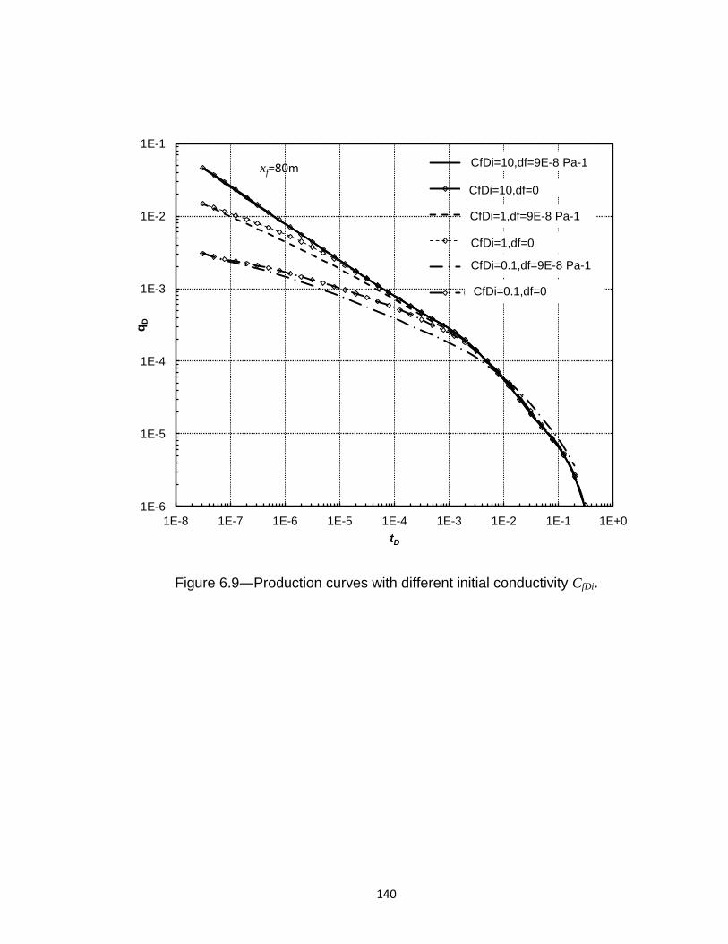
140
Figure 6.9―Production curves with different initial conductivity CfDi.
1E-6
1E-5
1E-4
1E-3
1E-2
1E-1
1E-8 1E-7 1E-6 1E-5 1E-4 1E-3 1E-2 1E-1 1E+0
qD
tD
CfDi=30,df=9E-8 Pa-1
CfDi=30, df=0
CfDi=3,df=9E-8 Pa-1
CfDi=3,df=0
CfDi=0.3,df=9E-8 Pa-1
CfDi=0.3, df=0
xf=80m CfDi=10,df=9E-8 Pa-1
CfDi=10,df=0
CfDi=1,df=9E-8 Pa-1
CfDi=1,df=0
CfDi=0.1,df=9E-8 Pa-1
CfDi=0.1,df=0
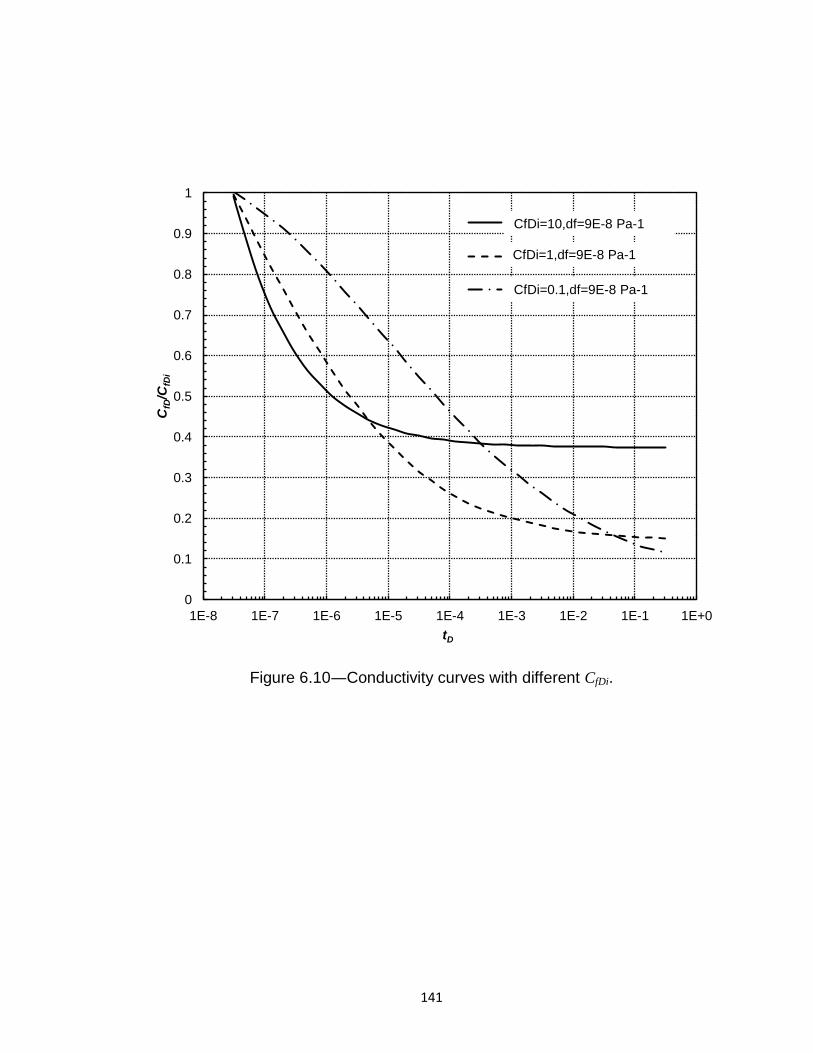
141
Figure 6.10―Conductivity curves with different CfDi.
0
0.1
0.2
0.3
0.4
0.5
0.6
0.7
0.8
0.9
1
1E-8 1E-7 1E-6 1E-5 1E-4 1E-3 1E-2 1E-1 1E+0
CfD
/CfD
i
tD
CfDi=30,df=9E-8 Pa-1
CfDi=3, df=9E-8 Pa-1
CfDi=0.3, df=9E-8 Pa-1
CfDi=10,df=9E-8 Pa-1
CfDi=1,df=9E-8 Pa-1
CfDi=0.1,df=9E-8 Pa-1

142
6.4 Field examples
This section presents two field case analyses using both the analytical
solutions and my semi-analytical models, which reveals each method’s strong
and weak points, respectively.
6.4.1 Marcellus shale gas well A
The original data from the Marcellus shale gas multi-stage fractured
horizontal well A were first reported by Nobakht et al. (2012a). The well is
producing under high-drawdown conditions (90%~95% drawdown), and,
therefore, the assumption of constant flowing pressure is applicable. The 10-
stage fractured horizontal well length is 1219 m (4000 ft). The properties of this
reservoir are as follows: pi=3.65×10⁷ Pa (5300 psi), T=339 K (150°F), h=38 m
(125 ft), ϕ=8%, Sg=76%, Sw=24%, and cf=7.25×10⁻¹⁰ Pa-1 (5×10⁻⁶ psi-1).
Figure 6.11 shows a plot of inverse gas rate vs. fourth root of time for this
well. The bilinear flow dominates during the production period. The straight line’s
slope is 0.4248 s0.75/m3. Using this slope and Equation (6.7b), the product of
square root of matrix permeability and fracture conductivity ff
wkk can be
estimated as 5.725×10⁻²⁷ m4. However, the production data deviates from the
straight line after t=1.27×10⁷ s (147 days) so the second plot of inverse gas rate
vs. square root of time (Figure 6.12) is provided to analyze late-time data. The
slope and intercept of the straight line are 4×10⁻⁴ s0.5/m3 and 1.2367 s/m3,
respectively.
143
Figure 6.11―Plot of reciprocal gas rate vs. fourth root of time.
0
0.5
1
1.5
2
2.5
3
3.5
4
4.5
5
0 10 20 30 40 50 60 70 80
1/q
, s/m
3
t0.25, s0.25
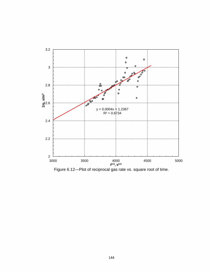
144
Figure 6.12―Plot of reciprocal gas rate vs. square root of time.
y = 0.0004x + 1.2367 R² = 0.6734
2
2.2
2.4
2.6
2.8
3
3.2
3000 3500 4000 4500 5000
1/q
, s/m
3
t0.5, s0.5

145
According to Equation (6.10b), f
xk can be calculated as 4×10⁻⁷ m2. In addition,
the fracture half-length is chosen to be 150 m from microseismic mapping. Then,
the matrix permeability and fracture conductivity should be 9×10-20 m2 (90 nd)
and 1.91×10⁻¹⁷ m2 (0.0626 md∙ft), respectively, by coupling ff
wkk andf
xk .
My semi-analytical model is also applied and is compared with the above
method in this production rate analysis. Figures 6.13(a) and 6.13(b) give the
matching results using the semi-analytical model. Matrix permeability, fracture
conductivity and fracture half-length are revaluated as 9.5×10⁻¹⁹ m2 (95 nd),
1.9×10⁻¹⁷ m2 (0.0626 md∙ft), and 120 m (394 ft). Good agreement is achieved in
the analysis results from semi-analytical modeling and analytical solutions. At
t=1×10⁹ s (11,574th day), boundary-dominated flow begins and the EUR
obtained using my semi-analytical is 8.84×10⁷ m3 (3.12 Bscf). Also, the EUR in
analytical solutions for a 30-year forecast is 1.11×10⁸ m3 (3.91 Bscf).
The method using analytical solutions is simple and fast in analyzing and
predicting production rates, especially in bilinear/linear flow regimes. Hence,
when dealing with fractured wells with recognizable flow regimes, the analytical
solutions could become a preferred candidate for production rate analysis.
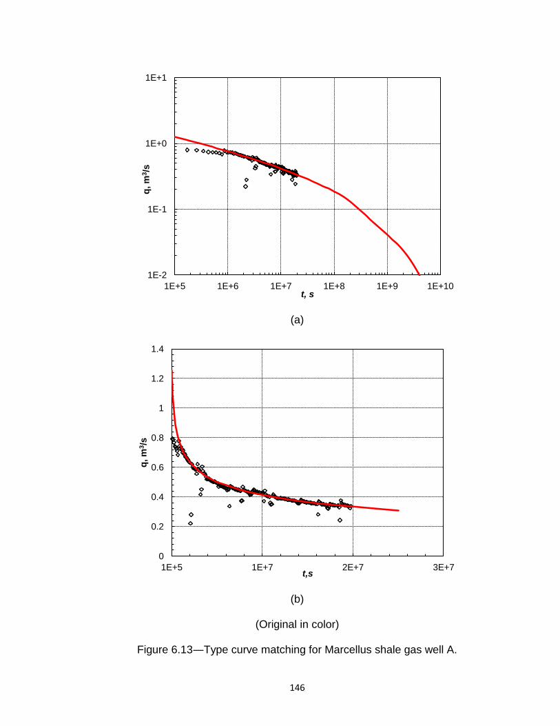
146
(a)
(b)
(Original in color)
Figure 6.13―Type curve matching for Marcellus shale gas well A.
1E-2
1E-1
1E+0
1E+1
1E+5 1E+6 1E+7 1E+8 1E+9 1E+10
q, m
3/s
t, s
0
0.2
0.4
0.6
0.8
1
1.2
1.4
1E+5 1E+7 2E+7 3E+7
q, m
3/s
t,s

147
6.4.2 Marcellus shale gas well B
This case study was introduced by Nobakht et al. (2012b) for a multi-stage
fractured horizontal well in the Marcellus shale gas reservoir. The well is 914 m
(3000 ft) long with 12 fractures. The reservoir properties are: pi=2.7×10⁷ Pa
(3924 psi), T=378 K (220°F), h=46 m (150ft), ϕ=7%, Sgi=66%, Swi=34%,
cf=5.8×10⁻¹⁰ Pa-1 (4×10⁻⁶ psi-1). Also, this well is producing under high-drawdown
conditions and could be considered as constant-pressure production. Moreover,
this case takes into account the gas desorption. According to Nobakht et al.’s
work (2012b), RD is set as 2.0.
The diagnostic plot, Figure 6.14, shows no typical flow regimes such as
bilinear and linear flow. I further investigated the relationship between inverse
production rate and square root of time for this case. Unlike the diagnostic plot,
a straight line can be drawn in Figure 6.15, which means linear flow appears.
The slope and intercept of the straight line are 3×10⁻⁴ s0.5/m3 and 0.378 s/m3.
With the line slope, Equation (6.10b) and matrix permeability 5×10-19 m2 (500 nd)
assumed by Nobakht (2012b), fracture half-length should be 110 m. The
intercept is the skin factor that reflects the reduced conductivity and changes the
shape of the log-log plot of q vs. t.
In order to verify these results, type curves of q vs. t are provided using my
semi-analytical model and parameters from Figure 6.15. However, although
dimensionless fracture conductivity CfD varies from 0.1 to 1, the type curves still
cannot match the field data because pseudo pseudo-steady state flow starts and
linear flow ends earlier than field data. Adjustments are necessary to analyze
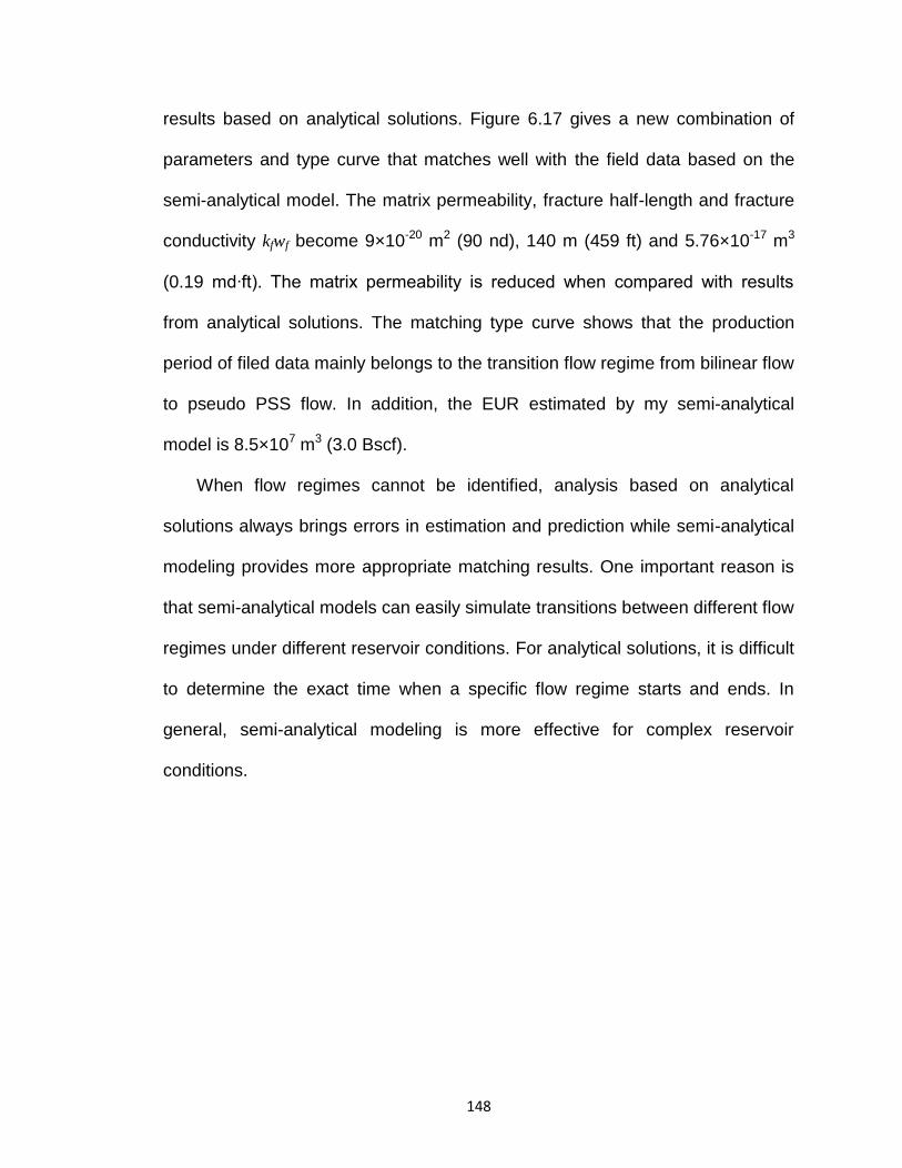
148
results based on analytical solutions. Figure 6.17 gives a new combination of
parameters and type curve that matches well with the field data based on the
semi-analytical model. The matrix permeability, fracture half-length and fracture
conductivity kfwf become 9×10-20 m2 (90 nd), 140 m (459 ft) and 5.76×10⁻¹⁷ m3
(0.19 md∙ft). The matrix permeability is reduced when compared with results
from analytical solutions. The matching type curve shows that the production
period of filed data mainly belongs to the transition flow regime from bilinear flow
to pseudo PSS flow. In addition, the EUR estimated by my semi-analytical
model is 8.5×10⁷ m3 (3.0 Bscf).
When flow regimes cannot be identified, analysis based on analytical
solutions always brings errors in estimation and prediction while semi-analytical
modeling provides more appropriate matching results. One important reason is
that semi-analytical models can easily simulate transitions between different flow
regimes under different reservoir conditions. For analytical solutions, it is difficult
to determine the exact time when a specific flow regime starts and ends. In
general, semi-analytical modeling is more effective for complex reservoir
conditions.
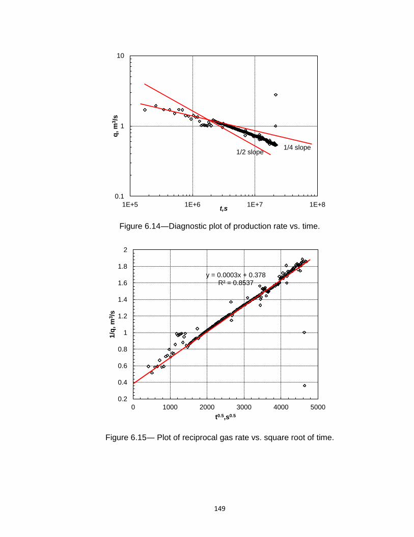
149
Figure 6.14―Diagnostic plot of production rate vs. time.
Figure 6.15― Plot of reciprocal gas rate vs. square root of time.
0.1
1
10
1E+5 1E+6 1E+7 1E+8
q, m
3/s
t,s
1/4 slope 1/2 slope
y = 0.0003x + 0.378 R² = 0.8537
0.2
0.4
0.6
0.8
1
1.2
1.4
1.6
1.8
2
0 1000 2000 3000 4000 5000
1/q
, m
3/s
t0.5,s0.5
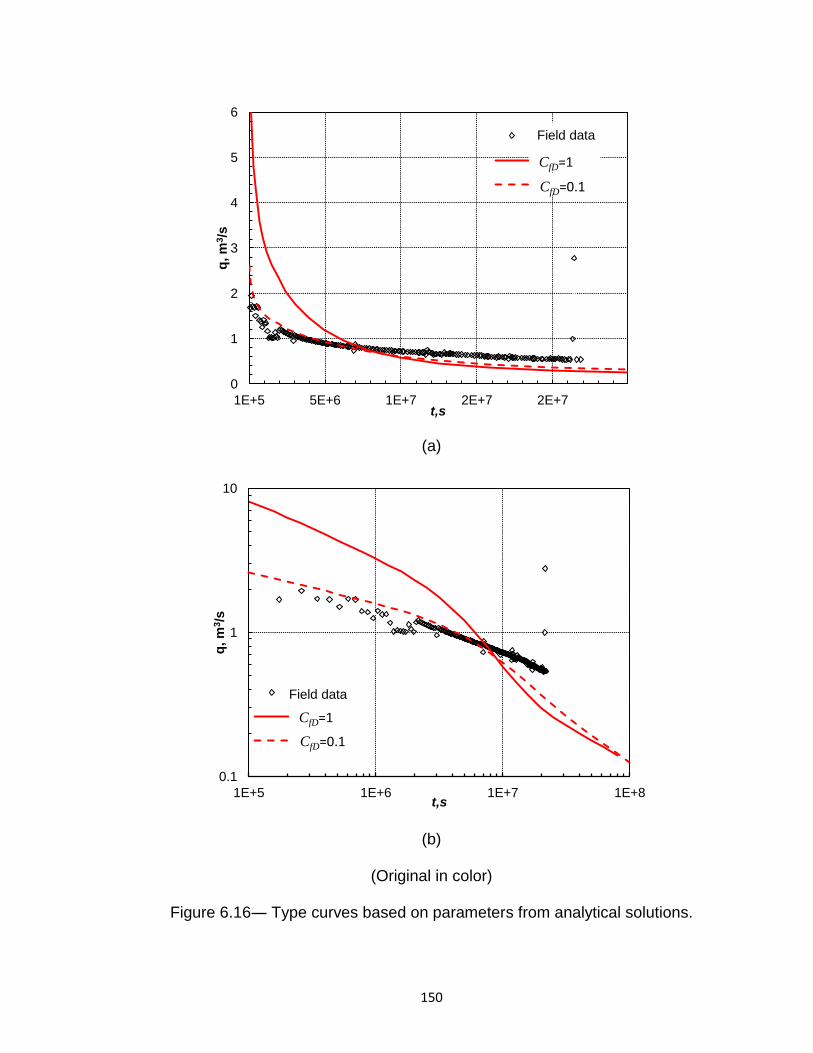
150
(a)
(b)
(Original in color)
Figure 6.16― Type curves based on parameters from analytical solutions.
0
1
2
3
4
5
6
1E+5 5E+6 1E+7 2E+7 2E+7
q, m
3/s
t,s
Series1
Series2
Series3
Field data
CfD=0.1
CfD=1
0.1
1
10
1E+5 1E+6 1E+7 1E+8
q, m
3/s
t,s
Series1
Series2
Series3
Field data
CfD=1
CfD=0.1
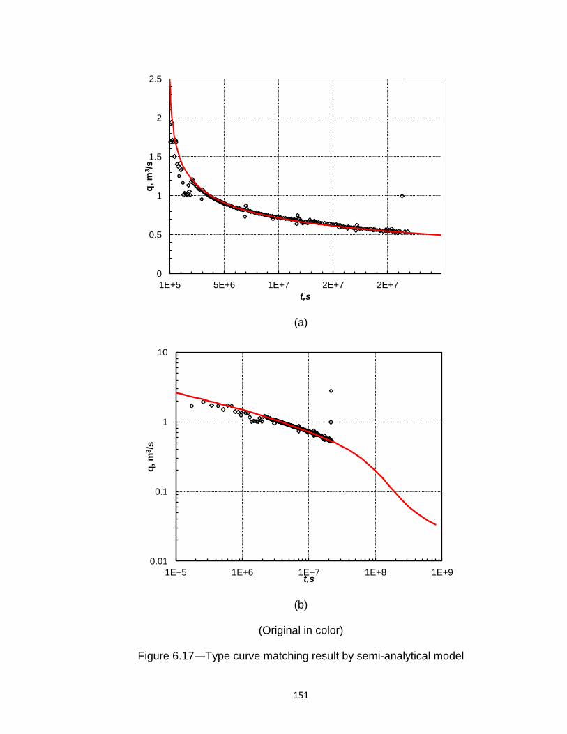
151
(a)
(b)
(Original in color)
Figure 6.17―Type curve matching result by semi-analytical model
0
0.5
1
1.5
2
2.5
1E+5 5E+6 1E+7 2E+7 2E+7
q, m
3/s
t,s
0.01
0.1
1
10
1E+5 1E+6 1E+7 1E+8 1E+9
q, m
3/s
t,s
152
6.5 Chapter summary
Transient production rate analysis provides another effective way to
evaluate reservoir properties and predict wells’ production in addition to transient
pressure analysis. In this Chapter, I developed a semi-analytical model for multi-
stage fractured horizontal wells with and without stress-sensitive fractures.
Moreover, the comparison between the semi-analytical model and analytical
solutions of different flow regimes reveals the mechanisms by which individual
fracture works.
The following conclusions are drawn from this study:
In bilinear and linear flow regimes, the fractured horizontal wells’
production is the sum of each fracture’s contribution.
The influence area of a fractured horizontal well is always larger than the
product of the horizontal well length and fracture half-length.
When considering stress-dependent hydraulic fracture conductivities, the
slope of bilinear flow becomes greater than 1/4 while linear flow’s slope
becomes smaller than 1/2.
The wells with smaller initial conductivity are more susceptible to stress-
dependent effects. Correspondingly, bilinear flow regime is more
sensitive to stress-sensitive fracture conductivities than other flow
regimes.
Analytical solutions are more suitable for production rate analysis with
recognizable flow regimes while semi-analytical modeling can deal with
complex reservoir problems with no clear signature of flow regimes.

153
CHAPTER 7
CONCLUSIONS AND RECOMMENDATIONS
7.1 Conclusions
The contributions of this work can be classified into the following categories:
methodology, transient pressure behaviour, and production rate analysis. The
results in each category are summarized as follows:
Methodology
1) I have introduced a general, effective, and accurate semi-analytical model
to investigate the transient pressure behaviour and transient production
rate behaviour of multi-stage fractured horizontal wells under constant
rate or pressure conditions. This methodology is as accurate as the
analytical method, as flexible and applicable as numerical models, and
also supports the stress-sensitive hydraulic fracture conductivities.
Transient pressure behaviour
2) For multi-stage fractured horizontal wells, fluid flow from the reservoir
directly to the wellbore and the pressure drop inside the wellbore could
have more obvious influence on pressure and flow distribution when
fewer fractures are created along the wellbore.
3) There exists an optimum fracture treatment design for a specific reservoir
instead of production simply being better with more and larger hydraulic
fractures. When the fracture half-length is constant, an optimal fracture
number can be obtained for the highest profit. When the total fracture

154
volume remains unchanged, I could also find the best combination of
fracture numbers and the fracture half-lengths.
4) When the stress-dependent hydraulic fracture conductivity is considered
for multi-stage fractured horizontal wells, slopes of bilinear and linear flow
deviate from 1/4 and 1/2, which helps to form a hump in the pressure
derivative curves.
5) Higher hydraulic fracture stress-sensitive characteristic df, lower minimum
fracture conductivity CfDmin, and lower initial fracture conductivity CfDi
make stress-sensitive fractures more susceptible to conductivity loss
when the stress field changes during production.
6) The type curve matching method based on my semi-analytical models is
powerful in analyzing the complex transient pressure behaviour of multi-
stage fractured horizontal wells in tight formations and shale reservoirs.
Production rate analysis
7) For multi-stage fractured horizontal wells, the total production equals the
sum of each separate fracture’s contribution during bilinear/linear flow
regimes.
8) Fractured horizontal wells with lower initial conductivities and larger
stress-sensitive characteristic df have more significant conductivity
reduction during constant-pressure production.
9) Analysis based on analytical solutions is preferable when flow regimes
are identifiable while analysis with semi-analytical modeling is more
appropriate for complex production rate behaviour.

155
7.2 Recommendations
The following recommendations for future work are made based on my work
in this study:
1) The models and/or the results presented in this work can be
extended to more complicated reservoir conditions, such as complex
fracture systems, boundary conditions for stimulated reservoir
volume, and dynamic matrix permeability.
2) This work can be further incorporated with seismic data to fully
describe fractures underground and their effect on transient pressure
behaviour.
3) A Large amount of experimental data should be studied to modify the
equations that describe the relationship between fracture
conductivities and stress.
4) A large number of cases should be studied to investigate the
relationship between pressure derivative curve slopes and stress-
sensitive characteristic for transient pressure and production rate
behaviour of fractured wells.
156
LIST OF REFERENCES
Abass H., Sierra L. and Tahini A., Optimizing Proppant Conductivity and
Number of Hydraulic Fractures in Tight Gas Sand Wells. This paper SPE
126159 was prepared for presentation at the SPE Saudi Arabia Section
Technical Symposium, Alkhobar, Saudi Arabia,9-11 May 2009.
Agarwal, R.G., Gardner, D.C., Kleinsteiber S.W. and Fussell, D.D., Analyzing
Well Production Data Using Combined Type Curve and Decline Curve
Analysis Concepts. Paper SPE 49222 was prepared for presentation at
the SPE Annual Technical Conference and Exhibition held in New
Orleans, Louisiana, 27-30 September 1998.
Al-Hussainy, R., Ramey Jr., H.J. and Crawford, P.B., The Flow of Real Gases
Through Porous Media. Journal of Petroleum Technology
(1966)18(5):624-636.
Arps, J.J., Analysis of Decline Curves. Trans. American Institute of Mining,
Metallurgical, and Petroleum Engineers (1944)160,228-247.
Azari, M., Soliman, M.Y., Wooden, W.O. and Hunt, J.L. Performance Prediction
for Finite-Conductivity Vertical Fractures. Paper SPE 22659 was prepared
for the presentation at the 66th Annual technical Conference and
Exhibition of the Society of Petroleum Engineers held in Dallas, TX,
October 6-9, 1991.
Babu, D.K. and Odeh, A.S., Productivity of A Horizontal Well. SPE Reservoir
Engineering (1989)4(4):417-421.
157
Bello, R.O. and Wattenbarger, R.A., Multi-stage Hydraulically Fractured Shale
Gas Rate Transient Analysis. Paper SPW 126854 was presented at the
SPE North Africa Techniacal Conference and Exhibition in Cairo, Egypt,
February 14-18 2010.
Ben E. L. and Spencer, C.W., "Gas in Tight Reservoirs-An Emerging Major
Source of Energy" in David G. Howell (ed.), The Future of Energy Gasses,
US Geological Survey, Professional Paper(1993)1570:233-252.
Berumen, S., Tiab, D., Effect of Pore Pressure on Conductivity and Permeability
of Fractured Rocks. This paper SPE 35694 was prepared for presentation
at the Western Regional Meeting held in Anchorage, Alaska, 22-24 May
1996.
Best, M.E. and Katsube, T., Shale Permeability and Its Significance in
Hydrocarbon Exploration. Geophysics(1995) 14 (3): 165-170.
Brown, G., The History of the Darcy-Weisbach Equation for Pipe Flow
Resistance. Environmental and Water Resources History: pp 34-43.
Carter, R.D., Type Curves for Finite Radial and Linear Gas Flow Systems:
Constant Terminal Pressure Case. Journal of Society of Petroleum
Engineers (1985) 25(5): 719-728.
Celis V., Silva, R., Ramones, M., Guerra, J. and Da Prat, G., A New Model for
Pressure Transient Analysis in Stress Sensitive Naturally Fractured
Reservoirs. SPE Advanced Technology Series 1994, 2 (1): 126-135.
158
Chen, C.C. and Raghavan, R., A Multiply-Fractured Horizontal Well in A
Rectangular Drainage Region. Journal of Society of Petroleum Engineers
(1997) 2(4): 455-465.
Cinco-Ley, H. and Meng, H.Z., Pressure Transient Analysis of Wells with Finite
Conductivity Vertical Fractures in Double Porosity Reservoirs. Paper SPE
18172 presented at the SPE Annual Technical Conference and Exhibition,
Houston, TX., 5-8 October, 1988.
Cinco-Ley, H. and Samaniego-V, F., Transient Pressure Analysis for Fractured
Wells. Journal of Petroleum Technology (1981) 33(9): 1749-1766.
Cinco-Ley, H., Samaniego-V, F. and Dominguez, A. N., Transient Pressure
Behavior for a Well with Finite-Conductivity Vertical Fracture. SPE Journal
(1978)18(4):253-264.
Cheng, Y., Lee, W.J. and McVay, D.A., Improving Reserves Estimates From
Decline-Curve Analysis of Tight and Multilayer Gas Wells. SPE Reservoir
Evaluation & Engineering (2008)11(5): 912-920.
Cipolla, C.L., Lolon, E.P., Erdle, J.C. and Tathed, V., Modeling Well
Performance in Shale-Gas Reservoirs. This paper SPE 125532 was
prepared for presentation at the 2009 SPE/EAGE Reservoir
Characterization and Simulation Conference held in Abu Dhabi, UAE, 19-
21 October 2009.
Clark J.B., A Hydraulic Process for Increasing the Productivity of Oil Wells.
Journal of Petroleum Technology(1949)1(1):1-8.

159
Clarkson, C.R., Pedersen, P.K., Tight Oil Production Analysis: Adaptation of
Existing Rate-transient Analysis Techniques. Paper CSUG/SPE 137352
was presented at the Canadian Unconventional Resources& International
Petroleum Conference held in Calgary, Alberta, Canada, 19-21 October
2010.
Clarkson, C.R., Qanbari, F., Nobakht, M., Heffner, L., Incorporating
Geomechanical Changes into Rate-transient analysis: Example from the
Haynesville Shale. This paper SPE 162526 was prepared for presentation
at the SPE Canadian Unconventional Resources Conference held in
Calgary, Alberta, Canada, 30 October-1 Nov 2012.
Cox, S.A., Gilbert, J.V., Sutton, R.P. et al., Reservoir Analysis for Tight Gas.
Paper SPE 78695 was prepared for the presentation at SPE Eastern
Regional Meeting in Lexington, Kenturky, U.S.A., 23-25 October 2002.
Duong, A.N., Rate-Decline Analysis for Fracture-Dominated Shale Reservoirs.
SPE Reservoir Evaluation &Engineering (2011)14(3): 377-387.
Fetkovich, M.J., Decline Curve Using Type Curves. Journal of Petroleum
Technology (1980)32(6):1065-1077.
Friedel, T., Mtchedlishvili, G., Behr, A. et al., Comparative Analysis of Damage
Mechanisms in Fractured Gas Wells. This paper SPE 107662 was
prepared for presentation at the European Formation Damage
Conference, Scheveningen, The Netherlands, 30 May-1Jun 2007.
160
Gringarten, A.C. and Ramey Jr., H.J., The Use of Source and Green’s Functions
in Solving Unsteady-Flow Problems in Reservoirs. Journal of Society of
Petroleum Engineers (1973) 13(5):285-296.
Gringarten, A.C., Ramey, Jr., H.J. and Raghavan, R. 1974. Unsteady-State
Pressure Distributions Created by A Well with A Single Infinite-
Conductivity Vertical Fracture. Journal of Society of Petroleum Engineers
(1974) 14(4): 347-360.
Guo, G. and Evans, R.D. A Systematic Methodology for Production Modeling of
Naturally Fractured Reservoirs Intersected by Horizontal Wells. This
paper presented at International Conference on Recent Advances in
Horizontal Well Applications, Calgary, Canada, 20-23 March 1994.
Herge, T., Hydraulically Fractured Horizontal Well Simulation. Paper SPE 35506
was presented at the European 3-D Reservoir Modeling Conference,
Stavanger, Norway, April 16-17, 1996.
Horne, R.N. and Temeng, K.O., Relative Productivities and Pressure Transient
Modeling of Horizontal Wells with Multiple Fractures. Paper SPE 29891
was presented at the SPE Middle East Oil Show, Bahrain, 11-14 March
1995.
Jones Jr., F.O., A Laboratory Study of the Effects of Confining Pressure on
Fracture Flow and Storage Capacity in Carbonate Rocks. Journal of
Petroleum Technology (1975) 27(1):21-27.
Kupchenko, C.L., Gault, B.W. and Mattar, L., Tight Gas Production Performance
Using Decline Curves. This paper SPE 114991 was prepared for
161
presentation at the CIPC/SPE Gas Technology Symposium Join
Conference held in Calgary, Alberta, Canada, 16-19 June 2008.
Liang, P., Thompson, J.M. and Mattar, L., Importance of the Transition Period to
Compound Linear Flow in Unconventional Reservoirs. Paper SPE 162646
was presented at the SPE Canadian Unconventional Resources
Conference in Calgary, Alberta, Canada, October 30-November 1, 2012.
Lin, J. and Zhu, D., Modeling Well Performance for Fractured Horizontal Gas
Wells. Paper SPE 130794 was presented at the CPS/SPE International
Oil & Gas Conference in Beijing, China, June 8-10, 2010.
Liu, X., Modeling of Cold Heavy Oil Production Wells. Ph.D. dissertation.
University of Regina, 2006.
Maley, S., The Use of Conventional Decline Curve Analysis in Tight Gas Well
Applications. SPE/DOE 13898 was presented at the SPE/DOE low
Permeability Gas Reservoirs in Denver, Colorado, May 19-22, 1985.
Mayerhofer, M.J., Lolon, E.P., Warpinski, N.R., Cipolla,C.L., Walser,D., and
Rightmire,C.M., What is Stimulated Reservoir Volume? SPE Production
&Operation, (2010)25(1): 89-98.
Medeiros, F., Ozkan, E. and Kazemi, H., Productivity and Drainage Area of
Fractured Horizontal Wells in Tight Gas Reservoirs. SPE Rreservoir
Evaluation & Engineering(2008)11(5):902-911.
Minkoff, S.E., Stone. C.M., Bryant, S., Peszynska, M. and Wheeler, M.F.,
Coupled Fluid Flow and Geomechanical Deformation Modeling. Journal of
Petroleum Science and Engineering (2003) 38 (1-2): 37-56.
162
Mitch, Alberta’s Cardium Formation: Oil Play Overview, from
http://www.beatingtheindex.com/alberta-cardium-formation-oil-play-
overview.
Newman, A.B., Heating and Cooling Rectangular and Cyclindrical Solids.
Industrial and Engineering Chemistry (1936) 28(5): 545-548.
Nobakht, M., Mattar, L. and Anderson, D.M., Simplified Forecasting of
Tight/Shale-Gas Production in Linear Flow. Journal of Canadian
Petroleum Technology (2012a)51(6): 476-486.
Nobakht, M., Clarkson, C.R. and Kaviani, D., New and Improved Methods for
Performing Rate-transient Analysis of Shale Gas Reservoirs. SPE
Reservoir Evaluation& Engineering (2012b)15(3): 338-350.
Olarewaju, J.S. and Lee, W.J., New Pressure-Transient Analysis Model for
Dual-Porosity Reservoirs. SPE Formation Evaluation (1989)4(3):384-390.
Ozkan, E., Brown, M.L., Raghavan, R. and Kazemi, H., Comparison of
Fractured Horizontal-Well Performance in Conventional and
Unconventional Reservoirs. Paper SPE 121290 was presented at the
SPE Western Regional Meeting, San Jose, California, USA, 24-26 March,
2009.
Ozkan, E. and Raghavan, R., New Solutions for Well-Test-Analysis Problems:
Part1-Analytical Considerations. SPE Formation Evaluation (1991) 6(3):
359-368.
Palacio, J.C. and Blasingame, T.A., Decline-Curve Analysis Using Type Curves-
Analysis of Gas Well Production Data. Paper SPE 25909 presented at the
163
Joint Rocky Mountain Regional and Low Permeability Reservoirs
Symposium, Denver, CO, April 26-28, 1993.
Pedrosa Jr., O.A. 1986, Pressure Transient Response in Stress Sensitive
Formations. The paper SPE 15115 was prepared for presentation at the
56th California Regional Meeting of the Society of Petroleum Engineers in
Oakland, C.A. April 2-4 1986.
Pedroso, C.A., Corrêa, A.C.F., Petrobrâs S.A., A New Model of A Pressure-
Dependent-Conductivity Hydraulic Fracture in A Finite Reservoir:
Constant Rate Production Case. The paper was prepared for presentation
at the fifth latin American and Caribbean Petroleum Engineering
Conference and Exhibition held in Rio de Hanairo, Brazil, 30 Aug-3 Sep.
1997.
Penmatcha, V.R. and Aziz, K., Comprehensive Reservoir/Wellbore Model for
Horizontal Wells. Journal of Society of Petroleum Engineers (1999)
4(3):224-234.
Poe Jr., B.D., Evaluation of Reservoir and Hydraulic Fracture Properties in
Geopressure Reservoirs. This paper SPE 64732 was prepared for
presentation at the SPE Internationial Oil and Gas Conference and
Exhibition in China held in Beijing, China, 7-10 November 2000.
Pratikno, H., Rushing, J.A. and Blasingame, T.A., Decline Curve Analysis Using
Type Curves-Fractured Wells. Paper SPE 84287 was presented at the
SPE Annual Technical Conference and Exhibition in Denver, Colorado,
USA, October 5-8, 2003.
164
Raghavan, R., Chen, C.C. and Agarwal, B., An analysis of Horizontal Wells
Intercepted by Multiple Fractures. SPE J. (1997) 2(3): 235-245.
Raghavan, R. and Chin, L.Y., Productivity Changes in Reservoirs with Stress-
dependent Permeability. Paper SPE 77535 presented at the SPE Annual
Technical Conference and Exhibition, San Antonio, Texas. 29 September-
2 October, 2002.
Raghavan, R., Scorer, J.D.T., and Miller, F.G., An Investigation by Numerical
Methods of the Effect of Pressure-dependent Rock and Fluid Properties
on Well Flow Tests. Journal of Society of Petroleum Engineering
(1972)12(3):267-275.
Ralph Veatch, Overview of Current Hydraulic Fracturing Design and Treatment
Technology- Part 1, Journal of Petroleum Technology (1983)35(4): 677-
687.
Ralph Veatch, Overview of Current Hydraulic Fracturing Design and Treatment
Technology- Part 2, Journal of Petroleum Technology(1983)35(5): 853-
864.
Robertson S. Generalized Hyperbolic Equation. Paper USMS 018731 was
provided to the SPE for distribution and publication. Unsolicited in1988.
Russell, D.G., and Truitt, N.E., Transient Pressure Behaviour in Vertically
Fractured Reservoirs. Journal of Petroleum Technology
(1964)16(10):1159-1170; Trans., American Institute of Mining,
Metallurgical, and Petroleum Engineers, Vol.231.
165
Rutqvist, J., Wu, Y.S., Tsang, C.F., Bodvarsson, G., A Modeling Approach for
Analysis of Coupled Multiphase Fluid Flow, Heat Transfer, and
Deformation in Fractured Porous Rock. International Journal of Rock
Mechanics and Mining Sciences (2002)39(4):429-442.
Samaniego, V.F., Brigham, W.E., and Miller, F.G., An Investigation of Transient
Flow of Reservoir Fluids Considering Pressure-dependent Rock and Fluid
Properties. Journal of Society of Petroleum Engineers(1977) 17(2):141-
150.
Stehfest, H., Numerical Inversion of Laplace Transforms; Communications of
ACM (1970)13(1):47-49.
Thompson, J.M., Nobakht, M., and Anderson, D.M., Modeling Well Performance
Data from Overpressured Shale Gas Reservoirs. Paper CSUG/SPE
137755 was presented at the SPE Annual Technical Conference and
Exhibition, Dallas, Texas, 9-12 October 2010.
United States Department of Energy, Shale Gas: Applying Technology to Solve
America’s Energy Challenges, Pittsburgh: National Energy Technology
laboratory (NETL), 2011.
Vairogs, J., Hearn, C.L., Dareing, D.W., and Rhoades, V.W., Effect of Rock
Stress on Gas Production from Low-permeability Reservoirs. Journal of
Petroleum Technology, Sept. (1971)23(9):1161-1167.
Valkó, P.P. and Amini, S., The Method of Distributed Volumetric Sources for
Calculating the Transient and Pseudosteady-State Productivity of
Complex Well-Fracture Configurations. Paper SPE106279 was presented
166
at the SPE Hydraulic Fracturing Technology Conference, College Station,
Texas, 29-31 January, 2007.
Wattenbarger, R.A., EI-Banbi, A.H., Villegas, M.E., Bryan, M.J., Production
Analysis of Linear Flow into Fractured Tight Gas Wells. Paper SPE 39931
was prepared for presentation at the SPE Rocky Mountain Regional/Low-
Permeability Reservoirs Symposium, Denver, 5-8 April 1998.
Yilmaz, O., Nur, A. and Nolen-Hoeksema, R., Pore Pressure Profiles in
Fractured and Compliant Rocks. Unsolicited in1991.
Zeng, F., Modeling of Non-Darcy Flow in Porous Media and Its Application. Ph.D.
dissertation. University of Regina, 2008.
Zeng, F and Zhao, G., 2009. A New Model for Reservoirs with Discrete Fracture
System. Paper 2009-064 was prepared for the Canadian International
Petroleum Conference in Calgary, Alberta, Canada, 16-18 June.
Zhang, J., Kamenov, A. Zhu, D. and Hill, A.D., Laboratory Measurement of
Hydraulic Fracture Conductivities in the Barnett Shale. Paper SPE
163839 was prepared for presentation at the SPE Hydraulic Fracturing
Technology Conference, Woodlands, Texas, USA, 4-6 February 2013.
Zhao, G., Well Testing of Complex Geometry Reservoirs, Ph.D. dissertation,
University of Tulsa, 1999.
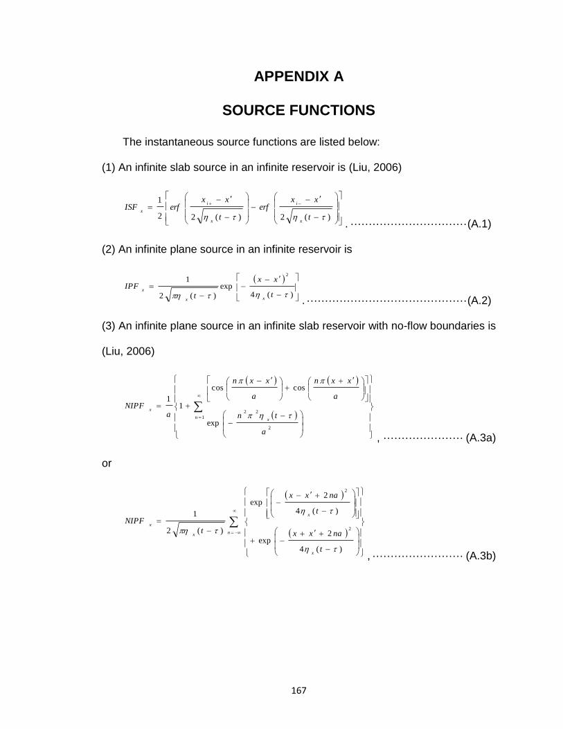
167
APPENDIX A
SOURCE FUNCTIONS
The instantaneous source functions are listed below:
(1) An infinite slab source in an infinite reservoir is (Liu, 2006)
)(2)(22
1
t
xxerf
t
xxerfISF
x
i
x
i
x
. ································ (A.1)
(2) An infinite plane source in an infinite reservoir is
)(4
exp
)(2
12
t
xx
t
IPF
xx
x
. ············································ (A.2)
(3) An infinite plane source in an infinite slab reservoir with no-flow boundaries is
(Liu, 2006)
1
2
22
exp
coscos
11
n x
x
a
tn
a
xxn
a
xxn
aNIPF
, ······················ (A.3a)
or
n
x
x
x
x
t
naxx
t
naxx
t
NIPF
)(4
2exp
)(4
2exp
)(2
1
2
2
, ························· (A.3b)
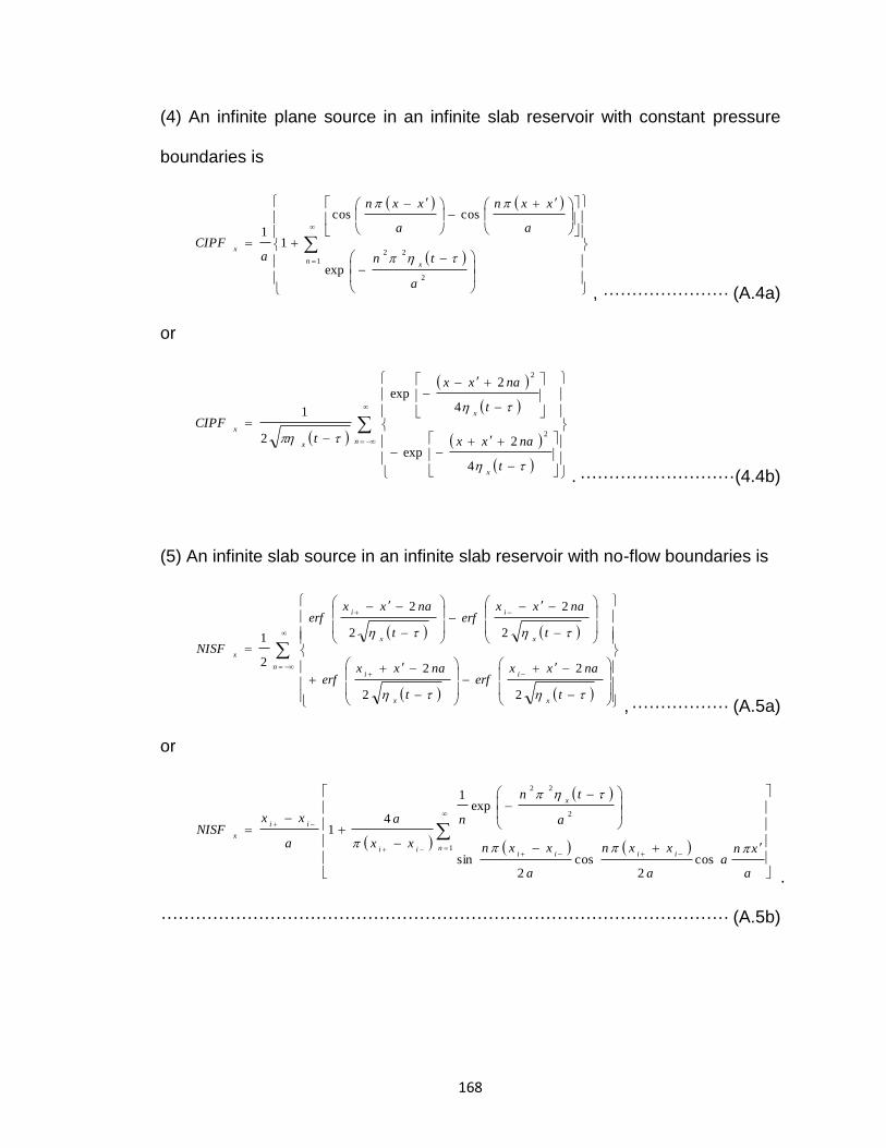
168
(4) An infinite plane source in an infinite slab reservoir with constant pressure
boundaries is
1
2
22
exp
coscos
11
n x
x
a
tn
a
xxn
a
xxn
aCIPF
, ······················ (A.4a)
or
n
x
x
x
x
t
naxx
t
naxx
t
CIPF
4
2exp
4
2exp
2
1
2
2
. ··························· (4.4b)
(5) An infinite slab source in an infinite slab reservoir with no-flow boundaries is
n
x
i
x
i
x
i
x
i
x
t
naxxerf
t
naxxerf
t
naxxerf
t
naxxerf
NISF
2
2
2
2
2
2
2
2
2
1
, ················· (A.5a)
or
1
2
22
cos2
cos2
sin
exp1
41
niiii
x
ii
ii
x
a
xna
a
xxn
a
xxn
a
tn
n
xx
a
a
xxNISF
.
··································································································· (A.5b)
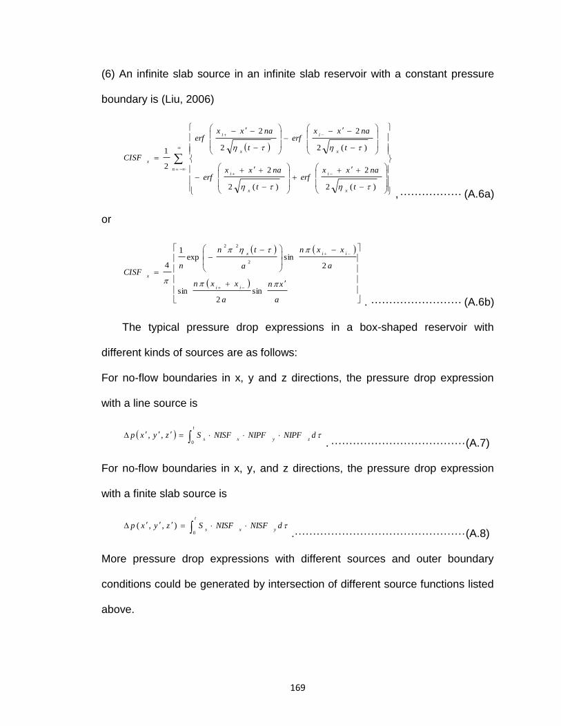
169
(6) An infinite slab source in an infinite slab reservoir with a constant pressure
boundary is (Liu, 2006)
n
x
i
x
i
x
i
x
i
x
t
naxxerf
t
naxxerf
t
naxxerf
t
naxxerf
CISF
)(2
2
)(2
2
)(2
2
2
2
2
1
, ················· (A.6a)
or
a
xn
a
xxn
a
xxn
a
tn
nCISF
ii
iix
x
sin2
sin
2sinexp
1
42
22
. ························· (A.6b)
The typical pressure drop expressions in a box-shaped reservoir with
different kinds of sources are as follows:
For no-flow boundaries in x, y and z directions, the pressure drop expression
with a line source is
dNIPFNIPFNISFSzyxpzy
t
xs 0
,,. ····································· (A.7)
For no-flow boundaries in x, y, and z directions, the pressure drop expression
with a finite slab source is
t
yxsdNISFNISFSzyxp
0
),,( .··············································· (A.8)
More pressure drop expressions with different sources and outer boundary
conditions could be generated by intersection of different source functions listed
above.
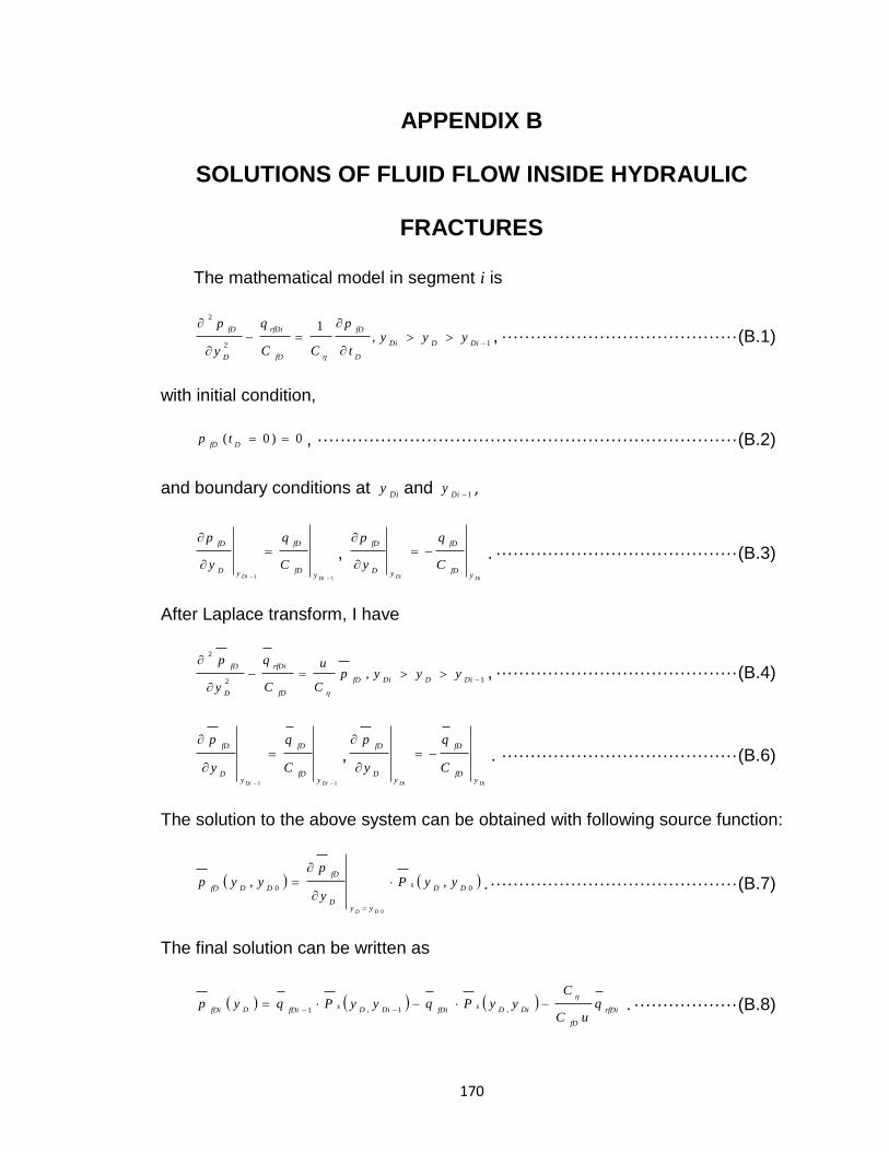
170
APPENDIX B
SOLUTIONS OF FLUID FLOW INSIDE HYDRAULIC
FRACTURES
The mathematical model in segment i is
12
2
,1
DiDDi
D
fD
fD
rfDi
D
fD
yyyt
p
CC
q
y
p
, ········································· (B.1)
with initial condition,
0)0( DfD
tp , ········································································· (B.2)
and boundary conditions at Diy and 1Di
y ,
11
DiDi yfD
fD
yD
fD
C
q
y
p
,
DiDi yfD
fD
yD
fD
C
q
y
p
. ·········································· (B.3)
After Laplace transform, I have
12
2
,
DiDDifD
fD
rfDi
D
fD
yyypC
u
C
q
y
p
, ·········································· (B.4)
11
DiDiy
fD
fD
yD
fD
C
q
y
p
,
DiDiy
fD
fD
yD
fD
C
q
y
p
. ········································· (B.6)
The solution to the above system can be obtained with following source function:
00
,,
0
DDs
yyD
fD
DDfDyyP
y
pyyp
DD
. ··········································· (B.7)
The final solution can be written as
rfDi
fD
DiDs
fDiDiDs
fDiDfDiq
uC
CyyPqyyPqyp
,1,1 . ·················· (B.8)
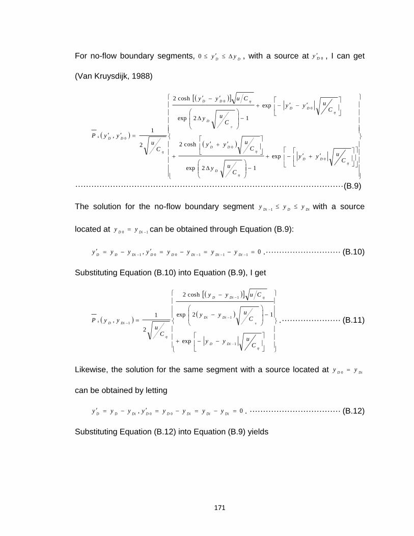
171
For no-flow boundary segments, DD
yy 0 , with a source at 0Dy , I can get
(Van Kruysdijk, 1988)
Cuyy
Cuy
Cuyy
Cuyy
Cuy
Cuyy
Cu
yyP
DD
D
DD
DD
D
DD
DDs
0
0
0
0
0
exp
12exp
cosh2
exp
12exp
cosh2
2
1,
···································································································· (B.9)
The solution for the no-flow boundary segment DiDDiyyy
1 with a source
located at 10
DiDyy can be obtained through Equation (B.9):
0,111001
DiDiDiDDDiDDyyyyyyyy . ···························· (B.10)
Substituting Equation (B.10) into Equation (B.9), I get
Cuyy
Cuyy
Cuyy
Cu
yyP
DiD
DiDi
DiD
DiDs
1
1
1
1
exp
12exp
cosh2
2
1, . ······················ (B.11)
Likewise, the solution for the same segment with a source located at DiDyy
0
can be obtained by letting
0,00
DiDiDiDDDiDD
yyyyyyyy . ·································· (B.12)
Substituting Equation (B.12) into Equation (B.9) yields
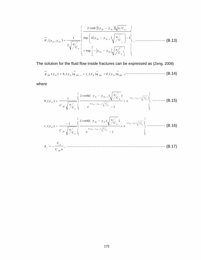
172
Cuyy
Cuyy
Cuyy
Cu
yyP
DiDi
DiDi
DiDi
DiDs
exp
12exp
cosh2
2
1,
1. ······················· (B.13)
The solution for the fluid flow inside fractures can be expressed as (Zeng, 2008)
rfDiDifDiDifDiDiDfDiqydqycqybyp )()()()(
1
, ······························· (B.14)
where
Cuyy
Cuyy
DiD
fD
Di
DiD
DiDi
e
e
Cuyy
CuC
yb
)(
)(2
11
1
1
])cosh[(21
)( ·········· (B.15)
Cuyy
Cuyy
DDi
fD
Di
DDi
DiDi
e
e
Cuyy
CuC
yc
)(
)(2
1
])cosh[(21
)(1
·············· (B.16)
uC
Cd
fD
i
. ············································································ (B.17)