Research ArticleModeling of Dual-Spinning Projectile with Canard andTrajectory Filtering

Jun Guan and Wenjun Yi

National Key Laboratory of Transient Physics, Nanjing University of Science and Technology, Nanjing 210094, China

Correspondence should be addressed to Jun Guan; guanjun8710@163.com

Received 27 March 2017; Accepted 2 January 2018; Published 11 April 2018

Academic Editor: Saad A. Ahmed

Copyright © 2018 Jun Guan andWenjun Yi. This is an open access article distributed under the Creative Commons AttributionLicense, which permits unrestricted use, distribution, and reproduction in any medium, provided the original work isproperly cited.

The article establishes a seven-degree-of-freedom projectile trajectory model for a new type of spinning projectile. Based on thismodel, a numerical analysis is performed on the ballistic characteristics of the projectile, and the trajectory of the dual-spinningprojectile is filtered with the unscented Kalman filter algorithm, so that the measurement information of projectile onboardequipment is more accurate and more reliable measurement data are provided for the guidance system. The numericalsimulation indicates that the dual-spinning projectile is mainly different from the traditional spinning projectile in that a degreeof freedom is added in the direction of the axis of the projectile, the forebody of the projectile spins at a low speed or even holdsstill to improve the control precision of the projectile control system, while the afterbody spins at a high speed maintaining thegyroscopic stability of the projectile. The trajectory filtering performed according to the unscented Kalman filter algorithm canimprove the accuracy of measurement data and eliminate the measurement error effectively, so as to obtain more accurate andreliable measurement data.

1. Introduction

With the technical development of weapons, basic require-ments of modern weapon systems are low collateral damageand accuracy. Currently, the great stocks of uncontrolledspin-stabilized projectiles in various countries are graduallybeing converted to precision-guided and controlled projec-tiles. Spin-stabilized projectiles maintain stability in flightthrough high-speed spinning. In order to deal with thechallenges to measurement and control systems caused byhigh-speed spinning, drag increasing mechanisms, spinningreducing mechanisms, pulse engines and built-in sliders,and similar components are currently used as actuators toreduce fall point dispersion effectively. However, the draw-back is that a continuous control force cannot be appliedand precision strikes are difficult to achieve.

At present, a canard-guided dual-spinning projectile[1–11] has been converted to a controlled spinning projectilewith great development potential. It can be used for continu-ous control to realize precision strikes. Furthermore, the great

amount of uncontrolled projectiles currently stored can bemodified into precise missiles only if fuzes of the traditionaluncontrolled spin-stabilized projectiles are changed intocanard-guided despinning fuzes. The dual-spinning projec-tile consists of two parts, that is, a forebody (with canards)and an afterbody, and the two parts are connected througha ball bearing. During flight, the forebody spins at a low speed(several or about a dozen turns per second), and the after-body spins at a high speed (hundreds of turns per second)around the vertical axis, which gives rise to the term “dual-spin.” The low spinning speed of the forebody can makethe measurement of related parameters and design of thecontrol system more precise, and the high spinning speedof the afterbody allows maintaining the gyroscopic stabilityof the projectile, achieving a stable flight. A structural dia-gram of a dual-spinning projectile is shown in Figure 1.

During flight, since the projectile is affected by factorssuch as the environment, certain errors will inevitably becaused in the measurement system. With accumulation ofthese errors, the precision of the control system will be greatly

HindawiInternational Journal of Aerospace EngineeringVolume 2018, Article ID 1795158, 7 pageshttps://doi.org/10.1155/2018/1795158

affected. Trajectory filtering based on flight measurementdata is an important means to understand the actual flightstatus of the projectile. It is widely applied in fields suchas simulated flight model validation, emplacement recon-naissance amending, and trajectory prediction and filtering[12, 13]. At present, extended Kalman filtering (EKF) iswidely applied in fields such as trajectory reconstructionand filtering. EKF is a linearization method for the nonlin-ear estimation problem. The linearization process will pro-duce certain errors; it is difficult to find out the Jacobimatrix in its analytical form for the dual-spinning projectilemodel; there also has a heavy calculation burden. In orderto overcome the shortcomings of EKF and avoid theerror-prone and calculation-heavy Jacobi matrix, recon-struction and filtering of the dual-spinning projectile’s tra-jectory in this article is performed using the unscentedKalman filter (UKF) [14–16].

2. Seven-Degree-of-Freedom MathematicalModel of Dual-Spinning Projectile

Since the spinning speeds of the forebody and the afterbodyof a dual-spinning projectile are different in the direction ofthe axis of the projectile, one degree of freedom (DOF) isadded to the six-DOF rigid body dynamic model, whichis used as a basis. Therefore, a seven-DOF dynamic modelof the dual-spinning projectile is established in this article.This model comprises a centroid motion caused by theresultant force and rotation around the centroid caused bythe resultant moment.

2.1. Coordinate System. The coordinate system of the axisof the projectile is as follows: The origin o is the locationof the centroid, the axis direction along the nose of theprojectile is the ox axis, the axis pointing rightward at aright angle to the axis of the projectile is the oy axis,and the oz axis is determined according to the right-

hand rule. Figure 2 is the schematic diagram of the coor-dinate system.

2.2. Dynamic Model. This article establishes a dynamic modelof the dual-spinning projectile under the coordinate systemof the axis of the projectile. This model comprises a dynamicmodel of the centroid motion and a dynamic model of therotation around the centroid. The model of the centroid’smotion is shown as (1), and the model of rotation aroundthe centroid is shown as (2).

u

v

w

= 1m

X

Y

Z

−

0 −r q

r 0 r tan θ

−q −r tan θ 0

u

v

w

,

1

Lf 0000

00

00

r−q

−r qq−r

−r tan �휃r tan �휃

LaMN

pfpaqr

= I−1 I .

r.q.pa.pf.

−

2

In (1) and (2), m is the total mass of the projectile;u, v,w are the velocity components, respectively; X, Y , Zare the resultant force components of the aerodynamicforce, the canard-guided control force, and the resultant forceof the Magnus force and gravity, respectively; pf , pa, q, rare the rotation speed components, where pf is the rotationspeed of the forebody and pa is the rotation speed of theafterbody; Lf , La,M,N are the moment components ofthe afterbody, where Lf indicates the rolling moment ofthe forebody and La indicates the rolling moment sub-jected contributed by the afterbody; while I is the momentof inertia matrix.

2.3. Kinematic Model. In the kinematic equation set of thedual-spinning projectile, kinematic equations of the move-ment of the centroid and the attitude change of the projectilebody relative to the ground coordinate system are estab-lished. Equation (3) is a kinematic model of the centroid ofthe dual-spinning projectile, and (4) is a kinematic modelof the attitude influenced by rotation around the centroid.

xe

ye

ze

=cos θ cos ψ −sin ψ sin θ cos ψcos θ sin ψ cos ψ sin θ sin ψ

−sin θ 0 cos θ

u

v

w

,

3tan �휃tan �휃

01/cos �휃

pfpaqr

.

�휓.�휃.�휙a.�휙f. 1

000

0100

0010

= 4

In (3) and (4), xe, ye, ze are the coordinate compo-nents in the ground coordinate system and ϕf , ϕa, θ, ψare the roll angle of the forebody, the roll angle of the

pfpa

Coaxial motor�훿3

�훿2

�훿1�훿4

Figure 1: Structural diagram of dual-spinning projectile.

o

y

z

x

Figure 2: The schematic diagram of the coordinate system.

2 International Journal of Aerospace Engineering

afterbody, the pitch angle, and the yaw angle of the pro-jectile body, respectively.

2.4. Force and Moment on Projectile

2.4.1. Force on Projectile. Resultant force is calculated asfollows:

X

Y

Z

=XB

YB

ZB

+XC

YC

ZC

+XM

YM

ZM

+XG

YG

ZG

5

Aerodynamic force from the projectile is calculatedas follows:

XB

YB

ZB

= qS

−CA α′, Ma

CYβ β, Ma β

−CNα α, Ma α

6

Aerodynamic force from the canard wing is calculatedas follows:

XC

YC

ZC

=0

CYδ Ma δy − β

−CNδ Ma δz + α

7

Magnus force is calculated as follows:

XM

YM

ZM

= padV

0−Cypα M α

Cypα M β

8

Gravity is calculated as follows:

XG

YG

ZG

=mg−sin θ

0cos θ

9

2.4.2. Moment on Projectile. Resultant moment is calculatedas follows:

Lf

La

M

N

=

LBf

LBa

MB

NB

+

LCf

LCa

MC

NC

+

LMf

LMa

MM

NM

+

LDf

LDa

MD

ND

+

LCFf

LCFa

MCF

NCF10

Moment from the projectile is calculated as follows:

LBfLBa qSd

00

MBCm�훼 (�훼, Ma) �훼Cm�훽 (�훽, Ma) �훽

=

NB

. 11

Moment from the canard wing is calculated as follows:

qSd

00

Cm�훿 (Ma)( �훿z + �훼)Cn�훿 (Ma)(�훿y − �훽)

=

LCfLCaMCNC

. 12

Magnus moment is calculated as follows:

Cnp�훼 (Ma) �훽Cnp�훼 (Ma) �훼

padV

LMfLMa −qSd

00

MMNM

= . 13

Damping moment is calculated as follows:

LDf

LDa

MD

ND

= qSddV

=

Clpf Ma pf

Clpa Ma pa

Cmq Ma q

Cnr Ma r

14

Control/friction moment is calculated as follows:

LCFf

LCFa

MCF

NCF

=

Lm + Lf‐a

−Lf‐a

00

, 15

where Lm is the control moment of the coaxial motor andLf‐a is the friction moment between the forebody and theafterbody, which can be expressed as

Lf‐a = qSdCAsgn pa − pf ks + kv pa − pf , 16

where ks is the static friction coefficient and kv is the viscousfriction coefficient.

In (5), (6), (7), (8), (9), (10), (14), (15), and (16), V =u2 + v2 +w2 is the total velocity of the missile body’s cen-

troid, d is the radius of the projectile, S is the reference area,q = 1/2 ρV2 is the dynamic pressure, and ρ is the air density;CA is the axial force coefficient, CYβ and CNα are the normalforce coefficients of the projectile body, CYδ and CNδ are thecanard wing lift coefficients, Cypα is the Magnus force coeffi-cient, and g is the gravitational acceleration; Cmα and Cmβ arethe normal moment coefficients of the projectile’s body, Cmδand Cnδ are the canard wing moment coefficients, Cnpα is theMagnus moment coefficient, Clpf and Clpa are the roll damp-ing moment coefficients of the forebody and the afterbody,respectively, and Cmq and Cnr are the equator damping

3International Journal of Aerospace Engineering

moment coefficients. δy and δz are the virtual equivalent rud-der angles, and the relationships between them and the realrudder angles are expressed with the following equations:

δz = cos ϕf δm − sin ϕf δn,δy = sin ϕf δm + cos ϕf δn,

17

where δm and δn are the pitch rudder angle and yaw steeringangle, respectively. α is the angle of attack, β is the angle ofsideslip, and α is the angle of total attack, and their equationsare as follows:

α = arctan wu,

β = arcsin vV

= arctan v

v2 +w2,

α′ = arccos uV

= arccos cos α cos β

18

3. Trajectory Characteristics

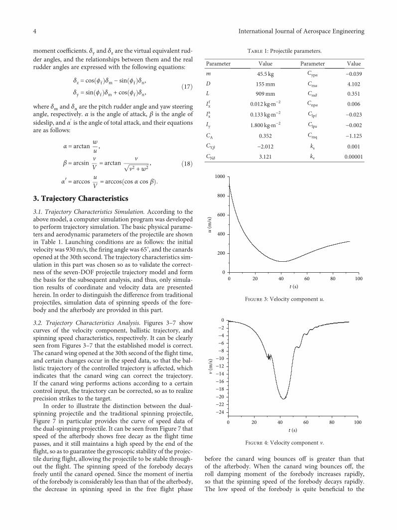
3.1. Trajectory Characteristics Simulation. According to theabove model, a computer simulation program was developedto perform trajectory simulation. The basic physical parame-ters and aerodynamic parameters of the projectile are shownin Table 1. Launching conditions are as follows: the initialvelocity was 930m/s, the firing angle was 65°, and the canardsopened at the 30th second. The trajectory characteristics sim-ulation in this part was chosen so as to validate the correct-ness of the seven-DOF projectile trajectory model and formthe basis for the subsequent analysis, and thus, only simula-tion results of coordinate and velocity data are presentedherein. In order to distinguish the difference from traditionalprojectiles, simulation data of spinning speeds of the fore-body and the afterbody are provided in this part.

3.2. Trajectory Characteristics Analysis. Figures 3–7 showcurves of the velocity component, ballistic trajectory, andspinning speed characteristics, respectively. It can be clearlyseen from Figures 3–7 that the established model is correct.The canard wing opened at the 30th second of the flight time,and certain changes occur in the speed data, so that the bal-listic trajectory of the controlled trajectory is affected, whichindicates that the canard wing can correct the trajectory.If the canard wing performs actions according to a certaincontrol input, the trajectory can be corrected, so as to realizeprecision strikes to the target.

In order to illustrate the distinction between the dual-spinning projectile and the traditional spinning projectile,Figure 7 in particular provides the curve of speed data ofthe dual-spinning projectile. It can be seen from Figure 7 thatspeed of the afterbody shows free decay as the flight timepasses, and it still maintains a high speed by the end of theflight, so as to guarantee the gyroscopic stability of the projec-tile during flight, allowing the projectile to be stable through-out the flight. The spinning speed of the forebody decaysfreely until the canard opened. Since the moment of inertiaof the forebody is considerably less than that of the afterbody,the decrease in spinning speed in the free flight phase

before the canard wing bounces off is greater than thatof the afterbody. When the canard wing bounces off, theroll damping moment of the forebody increases rapidly,so that the spinning speed of the forebody decays rapidly.The low speed of the forebody is quite beneficial to the

Table 1: Projectile parameters.

Parameter Value Parameter Value

m 45.5 kg Cypα −0.039

D 155mm Cmα 4.102

L 909mm Cmδ 0.351

I fx 0.012 kg·m−2 Cnpα 0.006

Iax 0.133 kg·m−2 Clpf −0.023

Iy 1.800 kg·m−2 Clpa −0.002

CA 0.352 Cmq −1.125

CYβ −2.012 ks 0.001

CNδ 3.121 kv 0.00001

0

200

400

600

800

1000

u (m

/s)

20 40 60 80 1000t (s)

Figure 3: Velocity component u.

−24−22−20−18−16−14−12−10

−8−6−4−2

0

v (m

/s)

20 40 60 80 1000t (s)

Figure 4: Velocity component v.

4 International Journal of Aerospace Engineering

normal operation of the measurement and control systems,which is the expected result.

4. Trajectory Filtering

4.1. Construction of UKF Equation. The system model of thedual-spinning projectile is strongly nonlinear. If a linear fil-tering method, for example, KF or EKF, is applied, large lin-earization error will be caused. Moreover, system equationsof seven-DOF are very complex, and it is hard to obtain theJacobi matrix in analytical form, so in this article, the UKFis used to perform online trajectory reconstruction.

Depending on the actual engineering needs, online datafiltering is mainly performed on coordinates xe, ye, ze inthis article, so x = xe ye ze

T is selected as the stateparameter, and the measurement parameters are the mea-sured coordinates’ information. According to (1), (2), (3),and (4), the UKF state equation and measurement equationcan be built, which are shown as

x = f x t , u t +GW t ,y t = h x t , u t + v t ,

19

where W is the system noise, v is the measurement noise,G is the system noise driving matrix, and y is the vector ofthe measurement value.

The steps for trajectory reconstruction using the UKF arethe following.

4.1.1. Initialization. The weighting factor wmi of sigma

point, the weighting factor wci of the corresponding vari-

ance, and the associated scale factor are shown in the fol-lowing equations:

λ = η2 na + κ − na, 20

wm0 = λ

na + λ, 21

wc0 =

λ

na + λ+ 1 − η2 + ε , 22

wmi =wc

i =1

2 na + λ, i = 1,… , 2na 23

In (20), (21), (22), and (23), subscripts 0 and i of theweighting factor correspond to 2na + 1 sigma points. na isthe dimension of state vector, λ is the parameter of the com-posite scale, η is the major scale factor determining distribu-tion scope of sigma points around the priori mean, and thetypical value is 10−3, 1 , while ε is the second scale factorfor stressing weights of the zero-order sigma points for calcu-lation of posterior covariance (for Gaussian distribution, theoptimal is ε = 2), and κ is the third scale factor, which is usu-ally taken as 0. In this article, we assume that the processnoise and measurement noise are both zero-mean Gaussianwhite noise, the process noise covariance matrix is Q, andthe measurement noise covariance matrix is R.

4.1.2. Calculating Sigma Point and Updating. Since approxi-mating the state distribution is easier than approximating

−2

0

2

4

6

8

w (m

/s)

20 40 60 80 1000t (s)

Figure 5: Velocity component w.

1200010000

80006000

40002000

0 0500

10001500

20002500

ye (m)

xe (m)

z e(m

)

10000

8000

6000

4000

2000

0

Figure 6: Flight trajectory.

pfpa

Canard open time

0 10 20 30 40 50 60 70 80 90 100 110 120−10t (s)

0

200

400

600

800

1000

1200

1400

1600

1800

2000

p (r

ad/s

)

Figure 7: Spinning rate properties.

5International Journal of Aerospace Engineering

the nonlinear function, the nonlinear propagation of randomstate variables can be completed through a determined sam-ple group. It is assumed that the external stimulation, theestimated value of the state vector x, and the variance matrixof estimated error at time k− 1 are known as uk−1, xk−1, andPk−1. In order to simplify the calculation process and separatethe process noise, the continuous state equation integral formis used for the sigma point predicted value. The calculationprocess of 2na + 1 group sample sigma point χk−1 and its pre-dicted value χk/k−1, predicted mean χk/k−1, and predictedvalue of the variance of the state parameter Pk/k−1 at time kare shown in

χk−1 = xk−1 xk−1 − na + λ Pk−1 xk−1 + na + λ Pk−1 ,

χk/k−1 = χk−1 +tk

tk−1

f χk−1, uk−1 dt,

xk/k−1 = 〠2na

i=0wm

i χi,k/k−1,

Pk/k−1 = 〠2na

i=0wc

i χi,k/k−1 − xk/k−1 χi,k/k−1 − xk/k−1Τ +Q

24

4.1.3. Measurement Updating. Predicted measurement valueγk/k−1 at the time of k − 1, mean value of predicted measure-ment yk/k−1, and state parameter and measurement predic-tion error variance matrix at time k − 1 are Pxyk, themeasurement prediction error variance matrix is Pyyk, thestate variable correction coefficient matrix is Kk, the stateerror variance matrix at time k is Pk, and the state estimatedvalue at time k is xk. The computational equations of theabove physical parameters are as follows:

γk/k−1 = h χk/k−1, uk−1 ,

yk/k−1 = 〠2na

i=0wm

i γi,k/k−1,

Pyyk = 〠2ne

i=0wc

i γi,k/k−1 − yk,k−1 γi,k/k−1 − yk,k−1Τ + R,

Pxyk = 〠2ne

i=0wc

i χi,k/k−1 − xk,k−1 γi,k/k−1 − yk,k−1Τ,

Kk = PxykP−1yyk,

Pk = Pk/k−1 −KkPyykKΤk ,

xk = xk/k−1 +Kk yk − yk/k−1

25

4.2. Simulation Verification. The trajectory filtering methodbased on the algorithm given in this article was validated.The validation conditions were as follows: the projectileinitial speed was 930, the firing angle was 65°, and theprojectile weight was 45.5 kg. The measured trajectoryvalue was simulated by adding Gaussian white noise tothe theoretical calculating value of the trajectory. Basedon this measured value, the effectiveness of the UKF

algorithm in the process of trajectory filtering was verified.Figures 8–10 show comparison curves of measurementsand reconstruction values of xe, ye, and ze, respectively.It can be seen from Figures 8–10 that the precision of mea-surement data of the ballistic trajectory filtering throughthe UKF algorithm was significantly improved and is suit-able for engineering applications.

5. Conclusions

The article establishes a seven-DOF projectile trajectorymodel of a dual-spinning projectile. After analyzing theballistic characteristics of the dual-spinning projectile withthe method of numerical simulation, it can be seen thatthe major distinction between the dual-spinning projectileand the traditional spinning projectile is that the forebodyand the afterbody show different spinning speed characteris-tics. This article specifically analyzes the reason causing thisphenomenon and advantages for using such a structure.

MeasuredFiltered

0

2000

4000

6000

8000

10000

12000

x e (m

)

20 40 60 80 1000t (s)

Figure 8: Coordinate xe comparison figure.

MeasuredFiltered

20 40 60 80 1000t (s)

−500

0

500

1000

1500

2000

2500y e

(m)

Figure 9: Coordinate ye comparison figure.

6 International Journal of Aerospace Engineering

Furthermore, in this article, filtering the trajectory of thedual-spinning projectile is performed by using the UKFalgorithm. Based on the comparison of the ballistic trajectorydata before and after filtering, it can be seen that the precisionof the measurement data is further improved, which canprovide more accurate and reliable basic data for engineer-ing applications.

Conflicts of Interest

The authors declare that they have no competing interests.

Acknowledgments

This work is supported by the National Natural ScienceFoundation of China under grant number 11472136.

References

[1] M. Costello and A. Peter, “Linear theory of a dual-spin projec-tile in atmospheric flight,” Journal of Guidance, Control, andDynamics, vol. 23, no. 5, pp. 789–797, 2000.

[2] P. Wernert, Stability Analysis for Canard Guided Dual-SpinStabilized Projectiles, AIAA-2009-5843, AIAA, Reston, 2009.

[3] S. J. Chang and Z. Y. Wang, “Analysis of spin-rate property fordual-spin-stabilized projectiles with canards,” Journal ofSpacecraft and Rockets, vol. 51, no. 3, pp. 958–966, 2014.

[4] D. L. Zhu and S. J. Tang, “Flight stability of a dual-spin projec-tile with canards,” Proceedings of the Institution of MechanicalEngineers, Part G: Journal of Aerospace Engineering, vol. 229,no. 4, pp. 703–716, 2015.

[5] S. Chang, “Dynamic response to canard control and gravity fora dual-spin projectile,” Journal of Spacecraft and Rockets,vol. 53, no. 3, pp. 558–566, 2016.

[6] W. Philippe and T. Spilios, “Modelling and stability analysisfor a class of 155 mm spin-stabilized projectiles with coursecorrection fuse (CCF),” in Proceedings of the AIAA Atmo-spheric Flight Mechanics Conference, Portland, Oregon, 2011.

[7] S. Theodoulis, V. Gassmann, P. Wernert, L. Dritsas, I. Kitsios,and A. Tzes, “Guidance and control design for a class of spin-

stabilized fin-controlled projectiles,” Journal of Guidance,Control, and Dynamics, vol. 36, no. 2, pp. 517–531, 2013.

[8] Y. Zhang and L. Xiao, “Simulation research on flight controlsystem of dual-spin projectile with fixed wing canards,” Com-puter Simulation, vol. 33, no. 3, pp. 80–85, 2016.

[9] C.-H. Lee and B.-E. Jun, “Guidance algorithm for projectilewith rotating canards via predictor-corrector approach,”in 2014 IEEE Conference on Control Applications(CCA),pp. 2072–2077, Antibes, Fance, 2014.

[10] J. Spagni, S. Theodoulis, and P. Wernert, “Flight control for aclass of 155 mm spin-stabilized projectile with reciprocatingcanards,” in AIAA Guidance, Navigation and Control Confer-ence, Minnesota, 2012.

[11] J. Rogers and M. Costello, “Design of a roll-stabilized mortarprojectile with reciprocating canards,” Journal of Guidance,Control, and Dynamics, vol. 33, no. 4, pp. 1026–1034, 2010.

[12] R. J. Yang and L. M. Wang, “Trajectory reconstruction usingradar measured data,” Journal of Ballistics China, vol. 23,no. 3, pp. 43–46, 2011.

[13] Y.Wang and D. Y. Zhou, “Real-time trajectory data processingalgorithm based on adaptive UKF,” Journal of Huazhong Uni-versity of Science & Technology, vol. 42, no. 9, pp. 68–71, 2014.

[14] S. J. Julier and J. K. Uhlmann, “Unscented filtering and non-linear estimation,” Proceeding of the IEEE, vol. 92, no. 3,pp. 401–422, 2004.

[15] S. J. Julier and J. K. Uhlman, “A new method for nonlineartransformation of means and covariance in filters and estima-tors,” IEEE Transactions on Automatic Control, vol. 45, no. 3,pp. 477–482, 2000.

[16] S. J. Julier, “The scaled unscented transformation,” in Pro-ceeding of the 2002 American Control Conference, p. 4555,Anchorage, 2002.

MeasuredFiltered

0

2000

4000

6000

8000

10000

12000

z e (m

)

100806040200t (s)

Figure 10: Coordinate ze comparison figure.

7International Journal of Aerospace Engineering

International Journal of

AerospaceEngineeringHindawiwww.hindawi.com Volume 2018

RoboticsJournal of

Hindawiwww.hindawi.com Volume 2018

Hindawiwww.hindawi.com Volume 2018

Active and Passive Electronic Components

VLSI Design

Hindawiwww.hindawi.com Volume 2018

Hindawiwww.hindawi.com Volume 2018

Shock and Vibration

Hindawiwww.hindawi.com Volume 2018

Civil EngineeringAdvances in

Acoustics and VibrationAdvances in

Hindawiwww.hindawi.com Volume 2018

Hindawiwww.hindawi.com Volume 2018

Electrical and Computer Engineering

Journal of

Advances inOptoElectronics

Hindawiwww.hindawi.com

Volume 2018

Hindawi Publishing Corporation http://www.hindawi.com Volume 2013Hindawiwww.hindawi.com

The Scientific World Journal

Volume 2018

Control Scienceand Engineering

Journal of

Hindawiwww.hindawi.com Volume 2018

Hindawiwww.hindawi.com

Journal ofEngineeringVolume 2018

SensorsJournal of

Hindawiwww.hindawi.com Volume 2018

International Journal of

RotatingMachinery

Hindawiwww.hindawi.com Volume 2018

Modelling &Simulationin EngineeringHindawiwww.hindawi.com Volume 2018

Hindawiwww.hindawi.com Volume 2018

Chemical EngineeringInternational Journal of Antennas and

Propagation

International Journal of

Hindawiwww.hindawi.com Volume 2018

Hindawiwww.hindawi.com Volume 2018

Navigation and Observation

International Journal of

Hindawi

www.hindawi.com Volume 2018

Advances in

Multimedia

Submit your manuscripts atwww.hindawi.com