Modeling Method of a Low-Pass Filter Based on … words: Wave matrix, bond graph modeling,...

American J. of Engineering and Applied Sciences 3 (4): 631-642, 2010 ISSN 1941-7020 © 2010 Science Publications

Corresponding Author: Hichem Taghouti, Laboratory of Analysis and Commands Systems, Department of Electrical Engineering, National Engineering School of Tunis, P.O. Box 37, 1002 Tunisia Tel: + 216 99 97 75 32

631

Modeling Method of a Low-Pass Filter Based on Microstrip T-Lines with

Cut-Off Frequency 10 GHz by the Extraction of its Wave-Scattering Parameters from its Causal Bond Graph Model

1Hichem Taghouti and 1,2Abdelkader Mami

1Laboratory of Analysis and Commands Systems, Department of Electrical Engineering, National Engineering School of Tunis, P.O. Box 37, 1002 Tunisia

2Laboratory of Electronic and High Frequency Circuits, Department of Physics, Faculty of Sciences of Tunis, 2092 Tunisia

Abstract: Problem statement: This study presented a jointly application of bond graph technique and wave-scattering formalism for a new realization called scattering bond graph model which has the main advantage to show up explicitly the different wave propagation. Approach: For that, we proposed to find the scattering matrix from the causal bond graph model of a low-pass filter based on Microstrip lines and with cut-off frequency 10 GHz, while starting with determination of the integro-differentials operators which is based, in their determination, on the causal ways and causal algebraic loops present in the associated bond graph model and which gives rise to the wave matrix which gathers the incident and reflected waves propagation of the studied filter. Results: The scattering parameters, founded from the wave matrix, will be checked by comparison of the simulation results. Conclusion: Thereafter, we use a procedure to model directly this scattering matrix under a special bond graph model form often called “Scattering Bond Graph Model”. Key words: Wave matrix, bond graph modeling, microstrip lines, integro-differentials operators

INTRODUCTION

The scattering or the wave-scattering formalism (Paynter and Busch-Vishniac, 1988) was used in vast physique fields such as the characterization of the electric circuits. Several work, since the invention of the bond graph approach (Di-Filippo et al., 2002), showed that the scattering formalism (Newton, 2002) constitutes an alternative approach for the physical systems modeling (Kamel and Dauphin-Tanguy, 1993). They pointed out on the one hand some properties and in particular the orthogonality of wave matrix (Magnusson, 2001) respectively the scattering matrix (Ferrero and Pirola, 2006) which respects intrinsically the causal relations and includes explicitly the conservation laws (Pedersen, 2003). They showed in addition that the scattering representation exists for systems having neither impedance nor admittance such as the junctions of Kirchhoff, the gyrateurs and the transformers (Patrick and Adrien, 2008). In addition, the bond graph language (Di-Filippo et al., 2002) is based on a graphic representation of the physical

systems. These representations are based on the identification and the idealization of the intrinsic characteristics of the physical environments and on the structuring of a complex physical system in the networks form (Belevich, 1968). Moreover, in physics, the analogies theory allows bond graph technique (Di-Filippo et al., 2002) to generalize the representation networks with all the traditional physics fields of the systems with localized and/or distributed (based on Microstrip lines) parameters (Byrnes et al., 1999). The propose of this study is to present and apply a new extraction method of the scattering parameters, which constitute the scattering matrix, of any physical systems while basing on its causal and reduced bond graph model (Taghouti and Mami, 2009). At first and after having to present the method, we propose to use the causal bond graph model of a low-pass filter based on Microstrip lines (distributed elements) (Trabelsi et al., 2003) to find, on the one hand, the integro-differentials operators (Khachatryan and Khachatryan, 2008) which based on the causal ways and algebraic loops present in the causal bond

Am. J. Engg. & Applied Sci., 3 (4): 631-642, 2010

632

graph model and, on the other hand, to extract the wave matrix (Magnusson, 2001) from these operators. Then, we extract directly the scattering parameters (Newton, 2002) from the found wave matrix (Magnusson, 2001) and, at the aim to validate the found results; we make a comparison by the simulation of these scattering parameters under a simple program and under the classic techniques of conception and simulation of the microwave circuits by using the HP-ADS software (Vendelin et al., 2005). Finally, we propose to build a special form of bond graph model often named “Scattering Bond GraphModel” (Kamel and Dauphin-Tanguy, 1996) which able to highlight these transmission and reflexion coefficients (Scattering parameters) (Duclos and Clement, 2003). Extraction method of the scattering parameters: The new extraction method of the scattering parameters (Newton, 2002) is an analytical method which makes it possible to establish, for a linear complex system, the scattering relations between a fixed entry and exit. However, this method implies the succession of the following stages: • Decomposition of the system (causal bond graph

model) in subsystems (causal bond graph sub-model) put in cascades which are characterized by their respective wave matrix (Magnusson, 2001)

• Calculating the total wave matrix (Magnusson, 2001) of the whole system by carrying out the product of the elementary wave matrices

• Finally, the application of a linear transformation to this total matrix for extracting the scattering parameters (scattering matrix) (Newton, 2002) characterizing the complex system

The step that we propose was thought in this objective and consists in establishing a systematic method which binds the bond graph technique (Di- Filippo et al., 2002) to the wave-scattering formalism (Paynter and Busch-Vishniac, 1988). This method is based on an algebro-graphic procedure (Amara and Scavarda, 1991) which uses the causal ways notions and the Mason’s rule (Bolton, 1999) applied to a causal bond graph transformed and reduced (Taghouti and Mami, 2009). Wave-scattering decomposition and representation of complex system: Generally, we can represent any complex system functioning in low or high frequency by the following model of the Fig. 1 where the process is represented by the quadripole Q with different wave

scattering. These three subsystems (source, quadripole (Q) and load) are inter-connected and communicate between them by the means of a power transfer which is done in a continuous way from the source to the load as Fig. 1 indicates it. It is considered that the process, in its quadripole form, is in complex form and can be decomposed to subsystems which are connected by the intermediary of the wave-scattering variables (Paynter and Busch-Vishniac, 1988) as Fig. 2 indicates it. The incident and reflected waves distribution, which is propagated from the source towards the load through the quadripole Q, can be translated by a matrix representation of the wave scattering variables like Fig. 3 indicates it, where W is the wave matrix. Let us consider the two processes A and B with share where the signal entering B is directed in the same direction as the outgoing signal of process A, a similar way, the outgoing signal of B is in the same direction as the signal entering a as Fig. 3 indicates it. If these two processes are coupled, the assumption of the power continuity (Paynter and Busch-Vishniac, 1988) will imply:

2A 1Ba b= (1)

2A 1Bb a= (2)

Fig. 1: Complex system representation with the wave scattering variables

Fig. 2: Wave scattering representation on the

decomposed quadripole Q

Fig. 3: Representation of the wave scattering variables


633

The aiA and aiB quantities entering the A and B processes are called incident waves in the same way, the quantities biA and biB associated with the signals leaving the A and B processes are called reflected waves (Duclos and Clement, 2003). Classically, we express the power circulating in a bond and connecting two systems in the shape of a product of the two variables effort (noted: ε) and flow (noted: ϕ) in reduced form (Amara and Scavarda, 1991):

2 2

i ii, i

a bP

2 2

= − = ε ϕ

(3)

2 2

i i i ii, i

a b a b

2 2

+ −− = ε ϕ

(4)

So we can introduce the following linear transformation:

i i i

i i i

1 1 a a1H

1 1 b b2

ε= = −ϕ

(5)

The linear opposite transformation of the H transformation allows the passage of the intrinsic variables effort and flows (ε,ϕ) with the wave variables (ai, bi) as the following relation indicates it:

i i i

i i i

1 1a 1H

1 1b 2

ε ε= = − ϕ ϕ

(6)

The processes A and B constitute two processes with 2-ports of entry and exit whose wave matrices are:

A A A A1 11 12 2A A A B1 21 22 2

b w w a

a w w b

=

(7)

B B B B1 11 12 2B B B B1 21 22 2

b w w a

a w w b

=

(8)

The chain of n processes with 2-ports of entry and exit, like Fig. 3 indicates it, constitutes a process with 2-ports of entry and exit where the global wave matrix W is:

(A) (B) (N) N (i)iW W * W *........* W W= = ∏ (9)

So:

1 11 12 2 2

1 21 22 2 2

b w w a a[W]

a w w b b

= =

(10)

The scattering parameters are given by the following scattering matrix:

1 11 12 1 2

2 21 22 2 2

b S S a a[S]

b S S b a

= =

(11)

The relations between these matrixes are given by these following equations:

111 21 22

112 21

121 12 11 22 21

122 11 21

W S *S

W S

W S S *S *S

W S *S

−

−

−

−

= −

=

= − − =

(12)

1

11 22 12

121 22

112 11 21 12 22

122 21 22

S W * W

S S

S W W * W * W

S W * W

−

−

−

−

=

=

= − =

(13)

Wave scattering parameters and causal bond graph model: It is considered that the process, in its quadruple form and which inserted between two particular ports P1 and P2 which represent respectively the entry (source) and the exit (load) of the complex system can be represented by the following bond graph model transformed and reduced such us: • ε1 and ε2 are respectively the reduced variable

(effort) at the entry and the exit of the system • φ1 and φ2 are respectively the reduced variable

(flow) at the entry and the exit of the system

i

0

Effort

Rε = (14)

i 0flow * Rϕ = (15)

These are the reduced Effort (e) and Flow (f) with respect to R0 (scaling resistance). and to establish the output-input analytical relations, the bond graph model of the studied system must be transformed, reduced and especially be causal since these relations rest on the concepts of causal way and causal algebraic loops which can comprise the reduced bond graph model.


634

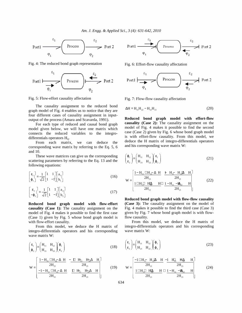
Fig. 4: The reduced bond graph representation

Fig. 5: Flow-effort causality affectation The causality assignment to the reduced bond graph model of Fig. 4 enables us to notice that they are four different cases of causality assignment in input-output of the process (Amara and Scavarda, 1991). For each type of reduced and causal bond graph model given below, we will have one matrix which connects the reduced variables to the integro-differentials operators Hij. From each matrix, we can deduce the corresponding wave matrix by referring to the Eq. 5, 6 and 10. These wave matrices can give us the corresponding scattering parameters by referring to the Eq. 13 and the following equations:

1 1

1 1

1 1 a1

1 1 b2

ε= −ϕ

(16)

2 2

2 2

1 1 a1

1 1 b2

ε= −−ϕ

(17)

Reduced bond graph model with flow-effort causality (Case 1): The causality assignment on the model of Fig. 4 makes it possible to find the first case (Case 1) given by Fig. 5 whose bond graph model is with flow-effort causality. From this model, we deduce the H matrix of integro-differentials operators and his corresponding wave matrix W:

1 11 12 1

2 21 22 2

H H

H H

ε ϕ= ϕ ε

(18)

11 22 11 22

21 21

11 22 11 22

21 21

1 H H H 1 H H H

2H 2HW

1 H H H 1 H H H

2H 2H

− + − ∆ − + − − ∆ = − − + − ∆ + − − ∆

(19)

Fig. 6: Effort-flow causality affectation

Fig. 7: Flow-flow causality affectation

11 22 12 21H H H H H∆ = − (20)

Reduced bond graph model with effort-flow causality (Case 2): The causality assignment on the model of Fig. 4 makes it possible to find the second case (Case 2) given by Fig. 6 whose bond graph model is with effort-flow causality. From this model, we deduce the H matrix of integro-differentials operators and his corresponding wave matrix W:

1 11 12 1

2 21 22 2

H H

H H

ϕ ε= ε ϕ

(21)

11 22 11 22

21 21

11 22 11 22

21 21

1 H H H 1 H H H

2H 2HW

1 H H H 1 H H H

2H 2H

− + − ∆ − − + ∆ = + + + ∆ + − − ∆

(22)

Reduced bond graph model with flow-flow causality (Case 3): The causality assignment on the model of Fig. 4 makes it possible to find the third case (Case 3) given by Fig. 7 whose bond graph model is with flow-flow causality. From this model, we deduce the H matrix of integro-differentials operators and his corresponding wave matrix W:

1 11 12 1

2 21 22 2

H H

H H

ε ϕ= ε ϕ

(23)

11 22 11 22

21 21

11 22 11 22

21 21

1 H H H 1 H H H

2H 2HW

1 H H H 1 H H H

2H 2H

− + − + ∆ − + − ∆ = + + + ∆ + − − ∆

(24)


635

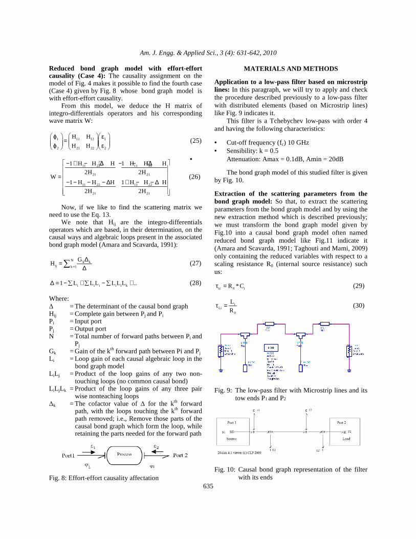
Reduced bond graph model with effort-effort causality (Case 4): The causality assignment on the model of Fig. 4 makes it possible to find the fourth case (Case 4) given by Fig. 8 whose bond graph model is with effort-effort causality. From this model, we deduce the H matrix of integro-differentials operators and his corresponding wave matrix W:

1 11 12 1

2 21 22 2

H H

H H

ϕ ε= ϕ ε

(25)

11 22 11 22

21 21

11 22 11 22

21 21

1 H H H 1 H H H

2H 2HW

1 H H H 1 H H H

2H 2H

− + − + ∆ − − + ∆ = − − − − ∆ + − − ∆

(26)

Now, if we like to find the scattering matrix we need to use the Eq. 13. We note that Hij are the integro-differentials operators which are based, in their determination, on the causal ways and algebraic loops present in the associated bond graph model (Amara and Scavarda, 1991):

N k kij k 1

GH

=

∆=∆∑ (27)

i i i i i k1 L L L L L L ..∆ = −∑ + ∑ − ∑ + (28) Where: ∆ = The determinant of the causal bond graph Hij = Complete gain between Pj and Pi Pi = Input port Pj = Output port N = Total number of forward paths between Pi and

Pj Gk = Gain of the kth forward path between Pi and Pj L i = Loop gain of each causal algebraic loop in the

bond graph model L iL j = Product of the loop gains of any two non-

touching loops (no common causal bond) L iL jLk = Product of the loop gains of any three pair

wise nonteaching loops ∆k = The cofactor value of ∆ for the kth forward

path, with the loops touching the kth forward path removed; i.e., Remove those parts of the causal bond graph which form the loop, while retaining the parts needed for the forward path

Fig. 8: Effort-effort causality affectation

MATERIALS AND METHODS Application to a low-pass filter based on microstrip lines: In this paragraph, we will try to apply and check the procedure described previously to a low-pass filter with distributed elements (based on Microstrip lines) like Fig. 9 indicates it. This filter is a Tchebychev low-pass with order 4 and having the following characteristics: • Cut-off frequency (fc) 10 GHz • Sensibility: k = 0.5

• Attenuation: Amax = 0.1dB, Amin = 20dB The bond graph model of this studied filter is given by Fig. 10. Extraction of the scattering parameters from the bond graph model: So that, to extract the scattering parameters from the bond graph model and by using the new extraction method which is described previously; we must transform the bond graph model given by Fig.10 into a causal bond graph model often named reduced bond graph model like Fig.11 indicate it (Amara and Scavarda, 1991; Taghouti and Mami, 2009) only containing the reduced variables with respect to a scaling resistance R0 (internal source resistance) such us:

ic 0 iR *Cτ = (29)

iLi

0

L

Rτ = (30)

Fig. 9: The low-pass filter with Microstrip lines and its

tow ends P1 and P2

Fig. 10: Causal bond graph representation of the filter

with its ends


636

• zi: The reduced equivalent impedance of the i element put in series

• yi: The reduced equivalent admittance of the i element put in parallel

So we have:

1 L1z * P= τ (31)

2 L2z * P= τ (32)

1 c1y * P= τ (33)

2 c2y * p= τ (34)

p: Laplace operator. The bond graph model given by Fig. 11 can be broken up into tow cells (sub-model) put in cascade form while respecting the assumption of the power continuity (Paynter and Busch-Vishniac, 1988) between all sub-models. Each cell is made up with an impedance z in parallel with an admittance y often noted [z---y], if the studied filter is with T form, or [y---z] if the studied filter is with Π form (type). So we have the first sub-model given by Fig. 12, this model is in conformity with case 1 described previously. So we have the integro-differentials operators by taking account to the previously equations:

11 1

1L : Loopgain of the algebraic loop

z y

−=

1 1

11 :Determinantof the associated causal bond graph

z y∆ = +

111

1 1

121 1

211 1

22

1 1

zH

z y 1

1H

z y 1

1H : Theall integro differentials operators

z y 1

y1H

z1y1 1

1H

z y 1

= +

=

+ = − + −=

+ −∆ =

+

Fig. 11: The transformed and reduced causal bond

graph model

Fig. 12: The first causal bond graph sub-model

Fig. 13: The second causal bond graph sub-model From these operators, we can deduce directly the wave matrix W(1) of the first sub-model of Fig. 12 by taking account to equations of case 1:

(1) 1 1 1 1 1 1 1 112

1 1 1 1 1 1 1 1

z y z y 2 z y z yW

z y z y z y z y

− − + − + += − − + + +

and now we have the second sub-model given by Fig. 13 and in the same manner we can extract the second wave matrix W(2) such us:


637

22 2

1L : Loopgain of the algebraic loop

z y

−=

2 2

11 : Determinantof the associated causal bond graph

z y∆ = +

211

2 2

122 2

212 2

222

2 2

2 2

zH

z y 1

1H

z y 1

1H : Theall integro differentials operators

z y 1

yH

z y 1

1H

z y 1

=

+ =

+ = − + − =

+ −∆ = +

and the second wave matrix is:

(2) 2 2 2 2 2 2 2 212

2 2 2 2 2 2 2 2

z y z y 2 z y z yW

z y z y z y z y

− − + − + += − − + + +

The total wave matrix W(T) is given by the product of the first and the second wave matrix such us:

(T) (1) (2) 11 12

21 22

w ww w * w

w w

= =

(35)

So the corresponding scattering matrix S(T) is given below:

1 122 12 11 21 12 22(T)

1 122 21 22

w *w w w * w * ws

w w * w

− −

− −

−=

− − (36)

From this matrix we can deduce these following scattering parameters:

1 2 1 2 1 2 1 2 1 1 2

2 1 2 1 211

z z y y z y (y z ) z (y y 1)

z (y y 1) y ys

d(p)

+ − + − − +

+ − + += (37)

12 21

2s s

d(p)= = (38)

The Fig. 11, represent the reduced bond graph model of the studied filter before decomposition. The Fig. 12 and 13 represent respectively the first and the second sub-model of the studied filter; they are

given by the decomposition of the reduced bond graph model of Fig. 11 at the appropriate bond (place).

1 2 1 2 1 2 1 2 1 1 2

2 1 2 1 222

z z y y z y (y z ) z (y y 1)

z (y y 1) y ys

d(p)

− + − + − − −

+ − + += (39)

1 2 1 2 1 2 1 2 1 2 2

2

d(p) z z y y z y (y z ) z (y z )

(y y1z1 z2 z1 z2\ y1 y2 21)

= − + − + +

+ + + + + = + + (40)

RESULTS

Thus, the validation is carried out by simulate the scattering parameters of Eq. 37-39. Simulation results and checking: A simple programming of the following scattering parameters equations, give the Fig. 14-17 which represent respectively the reflexion and transmission coefficients of the studied filter:

4 3C1 C2 L1 L2 L1 C2 C1 L2

2C1 L2 L1 C2 L2 L1

C1 C2 L1 L211 4 3

C1 C2 L1 L2 L1 C2 C1 L2

2C1 C2 L2 L1 C1 C2

L1 L2

p ( )p

[ ( ) ( )]P

( )pS

p ( )p

( )( )P (

)p 2

τ τ τ τ + τ τ τ − τ +

τ τ + τ + τ τ − τ +

τ + τ − τ − τ=τ τ τ τ + τ τ τ + τ +

τ + τ τ + τ + τ + τ

+ τ + τ +

(41)

4 3

C1 C2 L1 L2 L1 C2 C1 L2

2C2 L1 L2 C1 L1 L1

C1 C2 L1 L222 4 3

C1 C2 L1 L2 L1 C2 C1 L2

2C1 C2 L2 L1 C1 C2

L1 L2

p ( )p

[ ( ) ( )]P

( )pS

p ( )p

( )( )P (

)p 2

−τ τ τ τ + τ τ τ − τ +

τ τ − τ − τ τ + τ +

τ + τ − τ − τ=τ τ τ τ + τ τ τ + τ +

τ + τ τ + τ + τ + τ

+ τ + τ +

(42)

Fig. 14: Reflexion coefficient S11 seen at entry


638

Fig. 15: Transmission coefficient S12 seen from exit to

entry

Fig. 16: Transmission coefficient S21 seen from entry

to exit

Fig. 17: Reflexion coefficient S22 seen at exit

12 4 3C1 C2 L1 L2 L1 C2 C1 L2

2C1 C2 L1 L2 C1

C2 L1 L2

2S

p ( )p

( )( )P (

)p 2

=τ τ τ τ + τ τ τ + τ +

τ + τ τ + τ + τ +

τ + τ + τ +

(43)

Fig. 18: The low-pass filter under the HP-ADS software

Fig. 19: Simulation results of the low-pass filter

21 4 3C1 C2 L1 L2 L1 C2 C1 L2

2C1 C2 L1 L2 C1

C2 L1 L2

2S

p ( )p

( )( )P (

)p 2

=τ τ τ τ + τ τ τ + τ +

τ + τ τ + τ + τ +

τ + τ + τ +

(44)

We notice that the reflexions coefficients S11 and S22 are equal in module. This result is also checked by the figures below: 11 22S | | S |= (45)

To validate and checked the found results, by simulation, it is enough to simulate the low-pass filter of the Fig. 18 to find the representative curves of the reflexion and transmission coefficients respectively Sii and Sij by the HP-ADS software (Advanced Design System) (Jansen, 2003) often used in microwave and it is regarded as a traditional method in the line’s theory (Magnusson, 2001). The Fig. 18 thus represents the system's model studied with adapted entry and exit and the numerical values of its elements necessary for simulation. The simulation of the low-pass filter above gives the graphical representation of the reflexion and transmission coefficients Sii and Sij (i ≠ j and i, j = 1...2) according to the frequency like Fig. 19 indicate it.


639

By observing Fig. 19 and Fig. 14-17, we can say that our method of extracting the wave matrix from a reduced bond graph model is validated because it give us the same simulation results. Modeling of the scattering parameters with bond graph technique: We noted that we will use the method which is developed by Kamel and Dauphin-Tanguy (1993; 1996). Procedure used to model the scattering matrix by the bond graph technique: The scattering matrix of our studied process is a 2-2 matrix having a particular form whatever the expressions complexity of the series impedance or parallel admittance; it is orthogonal since the process is considered without loss and it admits the following general form:

11 n 11 12 n 12n 0 n 021 n 21 22 n 21n 0 n 0

n n 1n n 1

b p ... b b p ... b

b p ... b b p ... bS

a p a p ... ao−−

+ + + + + + + + =

+ + + (46)

We note that:

n n 1n n 1 0d(p) a p a p .... a−

−= + + + (47)

Indeed, if we consider the scattering matrix form found above for the process alone, we can say that it is not a true transfer matrix (Belevich, 1968) moreover, it is not in the adequate form since its various Sii parameters and sometimes Sij have the numerator’s degree equal to that of denominator and that poses a major problem to determinate the scattering bond graph model of any physical system studied in a general way. The solution with this problem is to regard the scattering matrix of a process as a transfer matrix from an input-output point of view, connecting the incident and the reflected waves in a symbolic system form. We start by carrying out an Euclidean division of each term of the numerator matrix (scattering parameters) by the common denominator d(p) what leads to the new shape of the scattering matrix (Breedveld, 1985) such as: S S' D= + (48) S’ = The new scattering matrix with degrees in the

numerator at most one less than that of d(s) D = Direct transmission matrix:

1 3

4 2

d dD

d d

=

(49)

Thereafter we seek for the new matrix S’ its development in continuous fraction in alpha-beta starting from the Routh method (Shamash, 1980) and build the corresponding bond graph model, since it is about a multivariable system (Molisch et al., 2002) while being based on the systematic procedure according to:

• Calculate the α-Routh table from the common

denominator d(p) and the β-Routh table from the new numerator of the S’-matrix

• Construct the direct chain by using the adequate number of elements I-C (which αi coefficients are their modules) in integral causality, equal to the degree of d(p)

• Duplicate this chain and construct the two entries of the quadruple

• Construct the tow outputs by using information bonds and a sufficient number of TF and GY elements whose modules are precisely the

ijnβ coefficients

• Add the direct part (transmission matrix D) by using information bonds

• To obtain the scattering bond graph model of the physical system, it is enough to add the reflexion

coefficient 0g

0

z 1P

z 1

−=

+ of the source and the

reflexion coefficient Lc

L

z 1P

z 1

−=+

of the load to the

scattering bond graph model of the process to the adequate sites

Scattering bond graph model of the low-pass filter: To obtain the scattering bond graph model of the studied circuit, it is enough to add the reflexion

coefficient 0g

0

z 1P

z 1

−=

+ of the source and the reflexion

coefficient Lc

L

z 1P

z 1

−=+

of the load to the scattering bond

graph model of the process to the adequate sites like Fig. 20 indicate it. It is interesting to notice that the structure of the scattering bond graph of the process remains the same whatever the degree of the common denominator of scattering matrix. The only thing that changes is the corresponding number of I and C linked to the α-Routh expansion (Kamel and Dauphin-Tanguy, 1993; 1996).


640

Fig. 20: Scattering bond graph model of the low-pass filter connecting to its source and load

3 2C2 L1 L2 L1 C2 L1 L2

11 4 3C1 C2 L1 L2 L1 C2 C1 L2 C1 C2

2L2 L1 C1 C2 L1 L2

2 p 2 P 2( )p 2S'

p ( )p ( )

( )P ( )p 2

τ τ τ + τ τ + τ + τ +=τ τ τ τ + τ τ τ + τ + τ + τ

τ + τ + τ + τ + τ + τ +

(50)

12 4 3C1 C2 L1 L2 L1 C2 C1 L2 C1 C2

2L1 L2 C1 C2 L1 L2

2S'

p ( )p ( )

( )P ( )p 2

=τ τ τ τ + τ τ τ + τ + τ + τ

τ + τ + τ + τ + τ + τ +

(51)

21 4 3C1 C2 L1 L2 L1 C2 C1 L2 C1 C2

2L1 L2 C1 C2 L1 L2

2S'

p ( )p ( )

( )P ( )p 2

=τ τ τ τ + τ τ τ + τ + τ + τ

τ + τ + τ + τ + τ + τ +

(52)

3 2

C2 L1 L2 L1 C2 L1 L222 4 3

C1 C2 L1 L2 L1 C2 C1 L2 C1 C2

2L2 L1 C1 C2 L1 L2

2 p 2 P 2( )p 2S'

p ( )p ( )

( )P ( )p 2

τ τ τ + τ τ + τ + τ +=τ τ τ τ + τ τ τ + τ + τ + τ

τ + τ + τ + τ + τ + τ +

(53)

1 0

D0 1

= −

(54)

The alpha-beta coefficients are then: From d(p) we have:

1 2 3 4, , andα α α α From S′11 we have:

11 11 11 111 2 3 4, , andβ β β β

From S′12= S′21 we have:

12 12 12 12 12 21 12 211 1 2 1 3 1 4 1, , and , andβ β β β β = β β = β

From S′22 we have:

22 22 22 221 2 3 4, , andβ β β β

DISCUSSTION

We sought to highlight the incident and reflected waves and their propagation on a bond graph called


641

“scattering bond graph” which, in addition to the simplicity of its structure which remains unchanged about or the complexity of the studied system, that it has a physical interpretation and easier to handle than an abstracted mathematical model and then it proposes a temporal approach phenomena usually modeled with the frequency tools. Moreover all the panoply of the techniques and properties of a bond graph can be used in a unified way with the service of a formalism which used from the low frequencies to highest. Moreover, this methodology which makes it possible to study simultaneously a given system with two complementary formalisms can supports us a broader comprehension of its behavior.

CONCLUSION In this study, we tried to present a method which appears new for the determination of the scattering parameters of any physical system functioning in high frequency. Then, we applied this technique to a low-pass filter based on Microstrip lines. Lastly, we validated the results found by a simple comparison between two methods of simulation: simulation by the traditional methods used in microwave under the HP-ADS software and simulation by our own method of the reduced bond graph which is based on the causal and simplified bond graph model of the studied system like on the minimum of the causal ways and loops present in this model often decomposed to sub-models as we showed previously. Generally, this new analysis method lead us, to use this new method which combines at the same time the bond graph technical and the scattering formalism for modeling and simulation of the scattering matrices of any electrical circuits often functioning in high frequency and based on localized or distributed elements giving rise to the famous model often named: Scattering bond graph. This new type of modeling will enable us to capture the power transfers in a simple and direct manner at the same time and it proposes us a temporal approach of the phenomena usually modeled with the frequencies tools.

ACKNOWLEDGMENT We make a point of thanking all those who contributed and aided for this work. We thank all the members of Laboratory of Analysis and Command Systems in particular Pr. Mami Abdelkader and Pr. Ksouri Mekki and without forgetting the members of the laboratory of electronics and high frequency circuits.

REFERENCES Amara, M. and S. Scavarda, 1991. A procedure to

match bond graph and scattering formalisms. J. Franklin Inst., 328: 887-899. DOI: 10.1016/0016-0032(91)90060-G

Belevich, V., 1968. Classical Network Theory. 1st Edn., Holden-Day, San Francisco, pp: 440.

Bolton, W., 1999. Newnes Control Engineering Pocketbook Control Engineering Pocketbook. Newnes, Oxford, ISBN: 10: 0750639288, pp: 304.

Breedveld, P.C., 1985. Multibond graph elements in physical systems theory. J. Franklin Inst., 319: 1-36. DOI: 10.1016/0016-0032(85)90062-6

Byrnes, C.I., D.S. Gilliam and V.I. Shubov, 1999. Boundary control, stabilization and zero-pole dynamics for a non-linear distributed parameter system. Int. J. Robust Nonlinear Control, 9: 737-768. DOI: 10.1002/(SICI)10991239(199909)9:11<77::AID-RNC432>3.0.CO;2-3

Di-Filippo, J.M., M. Delgado, C. Brie and H.M. Paynter, 2002. A survey of bond graphs: Theory, applications and programs. J. Franklin Inst., 328: 565-606. DOI: 10.1016/0016-0032(91)90044-4

Jansen, D., 2003. The Electronic Design Automation Handbook. 1st Edn., Springer, German, ISBN: 10: 14020 75022, pp: 680.

Duclos, G. and A.H. Clement, 2003. A new method for the calculation of transmission and reflection coefficients for water waves in a small basin. Comput. Rendus. Mecanique, 331: 225-230. DOI: 10.1016/S1631-0721(03)00053-6

Ferrero, A. and M. Pirola, 2006. Generalized mixed-mode s-parameters. IEEE Trans. Microwave Theory Tech., 54: 458-463. DOI: 10.1109/TMTT.2005.860497

Kamel, A. and G. Dauphin-Tanguy, 1993. Bond graph modeling of power waves in the scattering formalism. J. Simulat. Ser., 25: 41-41. http://direct.bl.uk/bld/PlaceOrder.do?UIN=005552011&ETOC=EN&from=searchengine

Kamel, A. and G. Dauphin-Tanguy, 1996. Power transfer in physical systems using the scattering bond graph and a parametric identification approach. Syst. Anal. Model. Simulat., 27: 1-13. http://portal.acm.org/citation.cfm?id=240821.240824

Khachatryan, K.H. and K.A. Khachatryan, 2008. Factorization of a convolution-type integro-differential equation on the positive half line. Ukrainian Math. J., 60: 1823-1839. DOI: 10.1007/s11253-009-0172-6

Magnusson, P.C., 2001. Transmission Lines and Wave Propagation. 4th Edn., CRC Press, USA., ISBN: 0849302692, pp: 519.


642

Molisch, A.F., M. Steinbauer, M. Toeltsch, E. Bonek and R.S. Thoma, 2002. Capacity of MIMO systems based on measured wireless channels. IEEE J. Selected Areas Commun., 20: 561-569. DOI: 10.1109/49.995515

Newton, R.G., 2002. Scattering Theory of Waves and Particles. 2nd Edn., Dover Publications, New York, ISBN: 10: 0486425355, pp: 768.

Patrick, J. and S. Adrien, 2008. Construction and analysis of improved Kirchhoff conditions for acoustic wave propagation in a junction of thin slots. ESAIM Proc. 25: 44-67. DOI: 10.1051/proc:082504

Paynter, H.M. and I.J. Busch-Vishniac, 1988. Wave- scattering approaches to conservation and causality. J. Franklin Inst., 325: 295-313. http://adsabs.harvard.edu/abs/1988FrInJ.235..295P

Pedersen, G., 2003. Energy conservation and physical optics for discrete long wave equations. Wave Motion, 37: 81-100. DOI: 10.1016/S0165-2125(02)00038-0

Shamash, Y., 1980. Stable biased reduced order models using the Routh method of reduction. Int. J. Syst. Sci., 11: 641-654. DOI: 10.1080/00207728008967043

Taghouti, H. and A. Mami, 2009. Application of the reduced bond graph approaches to determinate the scattering parameters of a high frequency filter. Proceeding of the 10th International Conference on Sciences and Techniques of Automatic Control and Computer Engineering, Dec. 20-22, Academic Publication Center Tunisia, Hammamet Tunisia, pp: 379-391.

Trabelsi, H., A. Gharsallah and H. Baudrand, 2003. Analysis of microwave circuits including lumped elements based on the iterative method. Int. J. RF Microwave Comput.-Aided Eng., 13: 269-275. DOI: 10.1002/mmce.10084

Vendelin, G.D., A.M. Pavio and U.L. Rohde, 2005. Microwave Circuit Design Using Linear and Non Linear Techniques. 2nd Edn., Wiley-Interscience, New York, ISBN: 13: 978-0471414797, pp: 1080.

Modeling Method of a Low-Pass Filter Based on … words: Wave matrix, bond graph modeling,...

Documents

Transcript of Modeling Method of a Low-Pass Filter Based on … words: Wave matrix, bond graph modeling,...