April 20, 2005

Modeling Inflation and Money Demand Using a Fourier-Series Approximation

Ralf Becker University of Manchester

Walter Enders*

University of Alabama

Stan Hurn Queensland University of Technology

Keywords: Nonlinear Time-Series, Fourier Approximation, Money Demand JEL Classification: E24, E31 * Corresponding author: Department of Economics, Finance and Legal Studies, University of Alabama, Tuscalooosa, AL 35487, wenders@cba.ua.edu. Ralf Becker was an Assistant Professor at Queensland University of Technology (QUT) and Walter Enders was a Visiting Professor at University of Technology Sydney (UTS) for part of the time they worked on this paper. They would like to thank QUT and UTS for their supportive research environments.

1

Modeling Inflation and Money Demand Using a Fourier-Series Approximation

1. Introduction

Consider the economic time-series model given by:

yt = αt + βxt + εt (1)

where: αt is the time-varying intercept, xt is a vector containing exogenous explanatory variables

and/or lagged values of yt, and εt is an i.i.d. disturbance term that is uncorrelated with any of the

series contained in xt. The notation in (1) is designed to emphasize the fact that the intercept term

is a function of time. Although it is possible to allow the value of β to be time-varying, in order

to highlight the effects of structural change, we focus only on the case in which the intercept

changes. If the functional form of αt is known, the series can be estimated, hypotheses can be

tested and conditional forecasts of the various values of {yt+j} can be made. In practice, two key

problems exist; the econometrician may not be sure if there is parameter instability and, if such

instability exists, what form it is likely to take. Parameter instability could result from any

number of factors including structural breaks, seasonality of an unknown form and/or an omitted

variable from a regression equation.

The time-series literature does address the first problem in great detail. In addition to the

standard Chow (1960) test and Hausman (1978) test, survey articles by Rosenberg (1973) and

Chow (1984) discuss numerous tests designed to detect structural change. More recently,

Andrews (1993) and Andrews and Ploberger (1994) have shown how to determine if there is a

one-time change in a parameter when the change point is unknown, Hansen (1992) has

considered parameter instability in regressions containing I(1) variables, Lin and Teräsvirta

2

(1994) showed how to test for multiple breaks, and Tan and Ashley (1999) formulated a test for

frequency dependence in regression parameters.

The second problem is more difficult to address since there are many potential ways to

model a changing intercept when the functional form of αt is unknown. For example, it is

possible to include dummy variables to capture seasonal effects or to represent one or more

structural breaks. Similarly, the inclusion of additional explanatory variables may capture the

underlying reason for the change in the intercept. The time-varying intercept may be estimated

using a Markov-switching process or a threshold process. Yet another avenue for exploration is

to let the data determine the functional form of αt. For example, the local-level model described

in Harvey (1989) uses the Kalman Filter to estimate αt as an autoregressive (or unit-root)

process. The purpose of this paper is to demonstrate how the misspecification problem can be

alleviated by the use of a methodology that ‘backs-out” the form of time-variation. The modeling

strategy is based on a Fourier approximation in that it uses trigonometric functions to

approximate the unknown functional form.

The choice of the Fourier approximation as the method for modeling the time-varying

intercept is driven by two major considerations. First, it is well-known that a Fourier

approximation can capture the variation in any absolutely integrable function of time. Moreover,

there is increasing awareness that structural change may often be gradual and smooth

(Leybourne et al., 1998, Lin and Teräsvirta, 1994), rather than the sudden and discrete changes

that are usually modeled by conventional dummy variables. As will become apparent, the

Fourier approximation is particularly adept at modeling this kind of time variation. Second, the

Fourier approach needs no prior information concerning the actual form of the time-varying

intercept αt. Traditional models using dummy variables or more recent developments based on

3

nonlinear deterministic time trends (Ripatti and Saikkonen, 2001) require that the form of the

time variation be specified at the outset. There is also a need to discriminate among alternative

specifications using standard diagnostic tools. As noted by Clements and Hendry (1998, pp. 168-

9), parameter change appears in many guises and can cause significant forecast error in practice.

They also establish that it can be difficult to distinguish model misspecification from the problem

of non-constant parameters.

The use of the Fourier approximation is now well established in the econometric

literature as Gallant (1984), Gallant and Souza (1991), and Becker, Enders and Hurn (2004) use

one or two frequency components of a Fourier approximation to mimic the behavior of an

unknown functional form. Moreover, the problem of testing for trigonometric components with

predetermined frequencies was tackled by Farley and Hinich (1970, 1975) in the context of a

model with parameter trend. Similarly, a test for the significance of trigonometric terms in a

regression equation with an unknown frequency component was introduced by Davies (1987). In

fact, Davies’ (1987) results are an important building block in our methodology. Davies’ test is

analogous to that of Tan and Ashley (1999) if their frequency band is restricted to a single

frequency.

There are many tests for parameter instability and it is not the intention of this paper to

merely present the empirical properties of yet another. Instead, our proposed methodology is

intended to be most helpful when it is not clear how to model the time-varying intercept. The

novel feature of this approach is that it uses the time-varying intercept as a modeling device to

capture the form of any potential structural breaks and, hence, lessen the influence of model

misspecification.

4

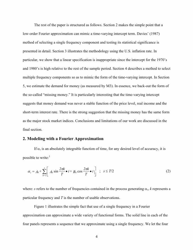
The rest of the paper is structured as follows. Section 2 makes the simple point that a

low-order Fourier approximation can mimic a time-varying intercept term. Davies’ (1987)

method of selecting a single frequency component and testing its statistical significance is

presented in detail. Section 3 illustrates the methodology using the U.S. inflation rate. In

particular, we show that a linear specification is inappropriate since the intercept for the 1970’s

and 1980’s is high relative to the rest of the sample period. Section 4 describes a method to select

multiple frequency components so as to mimic the form of the time-varying intercept. In Section

5, we estimate the demand for money (as measured by M3). In essence, we back-out the form of

the so-called “missing money.” It is particularly interesting that the time-varying intercept

suggests that money demand was never a stable function of the price level, real income and the

short-term interest rate. There is the strong suggestion that the missing money has the same form

as the major stock market indices. Conclusions and limitations of our work are discussed in the

final section.

2. Modeling with a Fourier Approximation

If αt is an absolutely integrable function of time, for any desired level of accuracy, it is

possible to write:1

; s ≤ T/2 (2)

where: s refers to the number of frequencies contained in the process generating αt, k represents a

particular frequency and T is the number of usable observations.

Figure 1 illustrates the simple fact that use of a single frequency in a Fourier

approximation can approximate a wide variety of functional forms. The solid line in each of the

four panels represents a sequence that we approximate using a single frequency. We let the four

••= ∑ t

Tk2 B + t

Tk2 A + A kk

s

1=k0t

ππα cossin

5

panels depict sharp breaks since the smooth Fourier approximation has the most difficulty in

mimicking such breaks. Consider Panel a in which the solid line represents a one-time change in

the level of a series containing 100 observations (T = 100). Notice that a single frequency such

that αt = 2.4 – 0.705sin(0.01226 t) – 1.82cos(0.01226 t) captures the fact that the sequence

increases over time (Note: k = 0.1953 and 2π*0.1953/100 = 0.01226). In Panel b, there are two

breaks in the series. In this case, the approximation αt = 0.642 – 0.105sin(0.586 t) –

0.375cos(0.586 t) captures the overall tendency of the series to increase. The solid line in Panel c

depicts a sequence with a temporary change in the level while the solid line in Panel d depicts a

“seasonal” sequence that is low in periods 1 – 25 and 51 – 75 and high in periods 26 – 50 and 76

– 100. Again, the approximations using a single frequency do reasonably well. It is interesting

that the frequency used for the approximation in Panel d is exactly equal to 2.0 since there are

two regular changes in the level of the sequence.

Note that the approximation can be improved by using more than one frequency. Suppose

that the solid line in Figure 2 represents a sequence that we want to estimate. If we approximate

this sequence with a single frequency (k = 1.171), we obtain the dashed line labeled “1

Frequency.” If we add another frequency component using k1 = 1.171 and k2 = 2.72, the

approximation is now depicted by the line labeled “2 Frequencies” in Figure 2.

Thus, each of these sequences can be approximated by a small number of frequency

components. The point is that the behavior of any deterministic sequence can be readily captured

by a sinusoidal function even though the sequence in question is not periodic. As such, the

intercept may be represented by a deterministic time-dependent coefficient model without first

specifying the nature of the nonlinearity. Since it is not possible to include all frequencies in (2),

the specification problem is to determine which frequencies to include in the approximation. As

6

a practical matter, the fact that we use a small number of frequencies means that the Fourier

series cannot capture all types of breaks. Figures 1 and 2 suggest that our Fourier approximation

will work best when structural change manifests itself smoothly.

Davies (1987) shows how to select the most appropriate single frequency and to test its

statistical significance. Suppose the {ξt} sequence denotes an i.i.d. error process with a unit

variance. Consider the following regression equation:

sin(2 / ) cos(2 / )t k k tA kt T B kt T eξ π π= + + (3)

where: Ak and Bk are the regression coefficients associated with the frequency k.

For any value of k, it should be clear that rejecting the null hypothesis Ak = Bk = 0 is

equivalent to rejecting the hypothesis that the { tξ } sequence is i.i.d. Since the frequency k is

unknown, a test of the null hypothesis involves an unidentified nuisance parameter. As such, it is

not possible to rely on standard distribution theory to obtain an appropriate test statistic. Instead,

if S(k) is the test statistic in question, Davies uses the supremum:

S(k*) = sup{S(k): L ≤ k ≤ U} (4)

where: k* = is the value of k yielding the largest value of S(k) and [ L, U ] is the range of possible

values of k.

Davies reparameterizes (3) such that:

Et-1(ξt) = a1sin[ ( t - 0.5T - 0.5)θ ] + b1cos[ ( t - 0.5T - 0.5 )θ ] (5)

where: θ = 2πk/T so that the values of {ξt} are zero-mean, unit-variance i.i.d. normally

distributed random variables with a period of oscillation equal to 2π/k (since θ = 2πk/T).

For the possible values of θ in the range [ L, U ] where 0 ≤ L < U ≤ π, construct:

2 2

1 21 1

( ) sin[( 0.5 0.5) ] / cos[( 0.5 0.5) ] /T T

t tt t

S k t T v t T vξ θ ξ θ= =

= − − + − − ∑ ∑ (6)

7

where: v1 = 0.5T - 0.5sin(Tθ)/sin(θ) and v2 = 0.5T + 0.5sin(Tθ)/sin(θ).

Davies shows that:

prob [ { S(k*): L ≤ θ ≤ U } > u ] (7)

can be approximated by:2

Tu0.5e-0.5u( U – L )/(24π)0.5 + e-0.5u (8)

Given T, U and L, critical values for S(k*) can be derived from equations (7) and (8).

Note that Davies’ method is equivalent to estimating (3) for each possible frequency in the

interval 0 < U – L ≤ T/2. The frequency providing the smallest residual sum of squares is the

same k* yielding the supremum S(k*). It is this value of k* that is a candidate for inclusion in the

time-varying intercept.

Becker, Enders and Hurn (2004) discuss a modified test version of the Davies (1987) test

that can be used in a regression framework. Let the data generating process be given by yt = β0 +

εt. To test for a structural break in the intercept, estimate the following regression equation by

ordinary least squares (OLS) for each potential frequency k:

yt = β0 + β1sin(2kπt/T) + β2cos(2kπt/T) + εt (9)

Let the value k* correspond to the frequency with the smallest residual sum of squares,

RSS*, and let *1β and *

2β be the coefficients associated with k*. Since the trigonometric

components are not in the data-generating process, *1β and *

2β should both equal zero. However,

the usual F-statistic for the null hypothesis * *1 2β β= = 0 does not follow a standard distribution

since the coefficients are estimated using a search procedure and k* is unidentified under the null

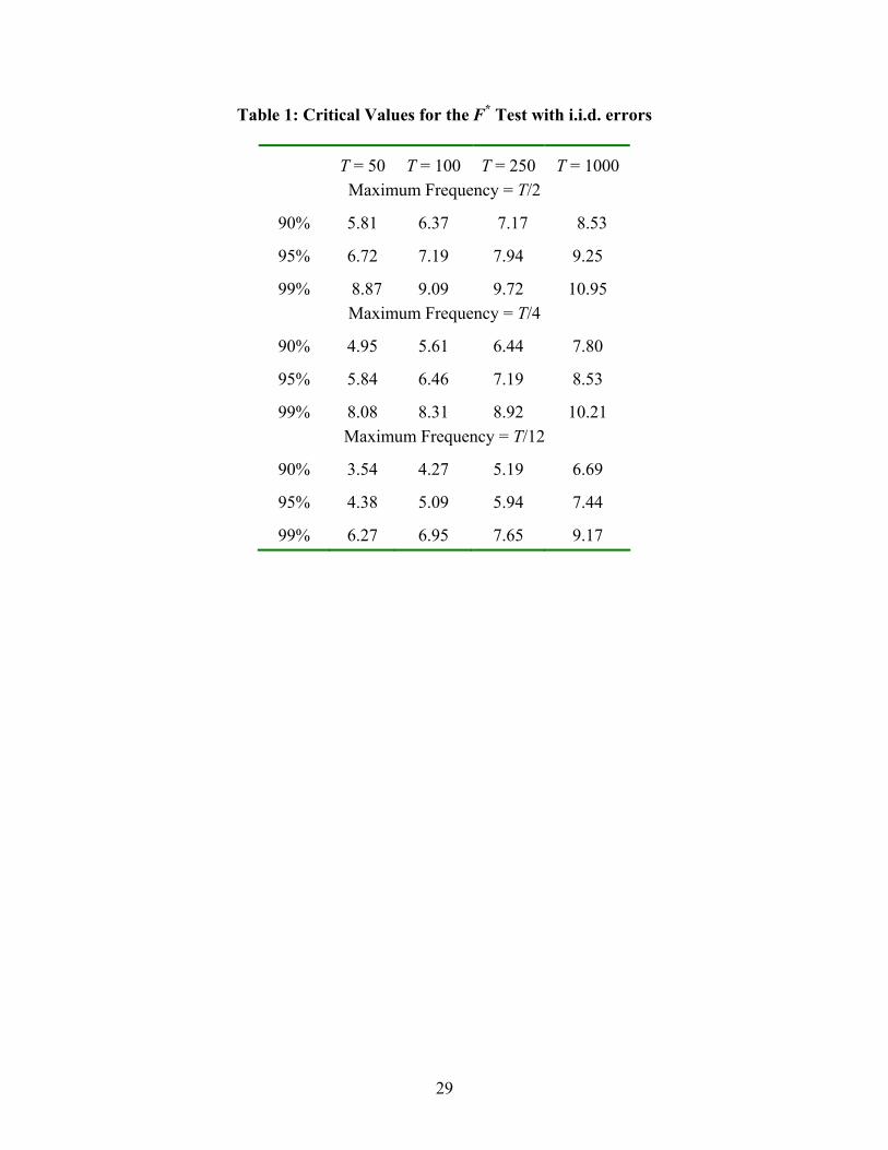
hypothesis of linearity. The critical values depend on the sample size and the maximum

frequency used in the search procedure; the critical values for the OLS procedure are reproduced

8

in Table 1. Note that this is a supremum test since k* yields the minimum residual sum of

squares.

2.2 Dependent error structures

It is not straightforward to modify the Davies test or the Trig-test for the case of a

dependent error process. Nevertheless, Enders and Lee (2004) develop a variant of the Trig-test

when the errors have a unit root. Suppose that {yt} is the unit-root process: yt = β0 + µt, where

µt = µt-1 + εt and that the researcher estimates a regression equation in the form of (9) by ordinary

least squares (OLS) for each potential frequency k. Enders and Lee (2004) derive the asymptotic

distribution of the F-test for the null hypothesis * *1 2β β= = 0. They tabulate critical values for

sample sizes of 100 and 500 searching over the potential frequencies to obtain the one with the

best fit (k*). As in Becker, Enders and Hurn (2004), their tabulated critical values, called F(k*),

depend on sample size and the maximum frequency used in the search procedure. It should be

clear that the F(k*) test is a supremum test since k* yields the minimum residual sum of squares.

For a sample size of 100 using a maximum value of k = 10, Enders and Lee (2004) report the

critical values of F(k*) to be 10.63, 7.78 and 6.59 at the 1%, 5%, and 10% significance levels,

respectively.

2.2 Power

Four conclusions emerged from Davies’ small Monte Carlo experiment concerning the

power of his test. First, for a number of sequences with structural breaks, the power of the test

increases in the sample size T. Second, the power of the test seems to be moderately robust to

non-normality. Third, if the frequency is not an integer, the use of integer frequencies entails a

loss of power. Fourth, if the frequency is an integer, the power of the discrete form of the test

exceeds that of the test using fractional frequencies. Moreover, as can inferred from equations

9

(7) and (8), increasing the size of U - L increases the probability of any given value of u. Thus,

unnecessarily expanding the size of the interval will reduce the power of the test. Since we are

considering a small number of structural breaks, it makes sense to use a small value of U since a

structural break is a ‘low frequency’ event.

It is well known that the most powerful test for a one-time change in the mean is that of

Andrews and Ploberger (AP) (1994). To further illustrate the power of Davies’ test, we

performed our own Monte Carlo analysis using equation (1) such that:

xt and εt ~ N(0,1), β = 1 and:

>∀≤∀

=40,40,0

tt

t δα (10)

We considered values of k in the range [ 0, 1 ] in order to allow for the possibility of an

infrequent change in the mean. After all, a frequency greater than one is not likely to replicate a

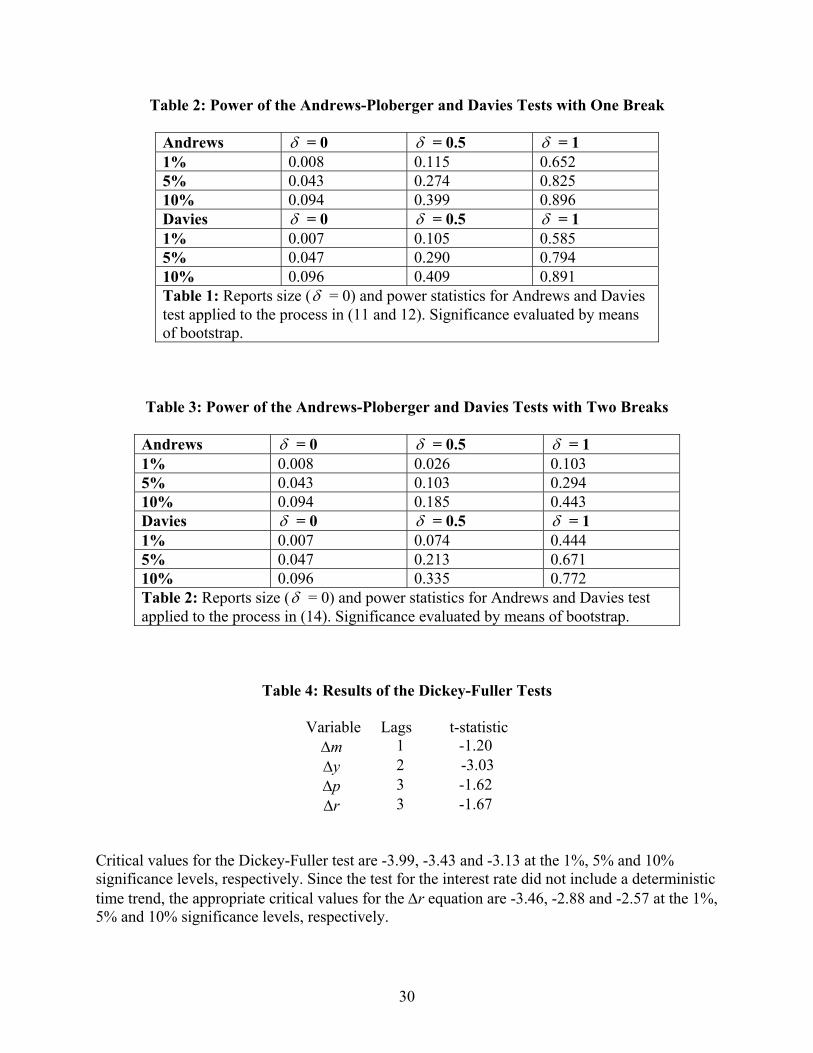
single break. Table 2 shows the power of the AP and the Davies tests for different break sizesδ .

Of course, if it is known that there cannot be more than a single break in the intercept, the

AP test is preferable to the Davies test. However, the Davies test does perform almost as well as

the optimal test for a single break. We performed a second Monte Carlo experiment to validate

the notion that a Fourier approximation can be especially useful to mimic a sequence with

multiple breaks. As such, we modified the data generating process in (9) to have a second

structural break:

>≤<

≤=

40,04020,

20,0

tt

t

t δα (11)

10

As shown in Table 3, the Davies test still possesses reasonably high power, while the AP

test has much weaker power compared to its power against a one time structural break.3 For

reasonably sized values of δ, the power of the Davies test exceeds that of the AP test.

Finally, Becker, Enders and Hurn (2004) show that Davies’ test and their modification of

the Davies’ test (called the Trig-test) can have more power than the Bai-Perron (1998) test when

the number of breaks is unknown. They show that the Davies test and the Trig-test have the

correct empirical size and excellent power to detect structural breaks and stochastic parameter

variation of unknown form.

3. A Structural Break in the Inflation Rate

To illustrate the use of the test for a single frequency component, we update and extend

the example of Becker, Enders and Hurn (2004). We consider the application of the test to

multiple frequencies in Section 4. In order to use the test it is necessary to standardize the

residuals to have a unit variance.4 A more important issue is that regression residuals are only

estimates of the actual error process. Hence, an alternative to obtaining critical values from (7)

and (8) is to bootstrap the S(k*) statistic. In order to illustrate the use of Davies’ test, we obtained

monthly values of the U.S. CPI (seasonally adjusted) from the website of the Federal Reserve

Bank of St. Louis (http://www.stls.frb.org/fred/index.html) for the 1947:1 to 2004:8 period. It is

well known that inflation rates, measured by the CPI, act as long-memory processes. For

example, Baillie, Han and Kwon (2002) review a number of papers indicating that U.S. inflation

is fractionally integrated and Clements and Mizon (1991) argue that structural breaks can explain

such findings; a break in a time-series can cause it to behave like a unit-root process.

11

If we let πt denote the logarithmic change in the U.S. CPI, the following augmented

Dickey-Fuller test (with t-statistics in parentheses) shows that the unit-root hypothesis can be

rejected for our long sample:5

∆πt = 0.603 – 0.173πt-1 + 11

1i

i

β=∑ ∆πt-i + et (12)

(3.17) (-4.35)

The key point to note is that standard diagnostic checks of the residual series {et} indicate

that the model is adequate. If ρi denotes the residual autocorrelation for lag i, the correlogram is:

ρ1 ρ2 ρ3 ρ4 ρ5 ρ6 ρ7 ρ8 ρ9 ρ10 ρ11 ρ12 -0.007 0.013 0.034 -0.008 0.002 0.051 -0.019 0.012 0.028 -0.012 -0.039 0.077

However, when we performed a Dickey-Fuller test using a more recent sample period

(1973:1 - 2004:8), the unit-root hypothesis cannot be rejected. Consider:

∆πt = 0.440 – 0.095πt-1 + 11

1i

i

β=∑ ∆πt-i + et (13)

(1.72) (-2.08)

In order to determine why the unit-root hypothesis is rejected over the entire sample

period but not the latter period, we performed additional diagnostic checks on (12). For example,

the RESET test suggests that the relationship is nonlinear. Let ∆ ˆtπ and t̂ε denote the fitted

values and the residual values of equation (12), respectively. We regressed t̂ε on all of the

‘explanatory’ variables in (12) and on ∆ ˆ Htπ . The idea of the RESET test is that this regression

should have little explanatory power if the actual data generating process is linear. For values of

H equal to 3, 4 and 5, the prob-values for the RESET test are 0.011, 0.002 and 0.000,

respectively. Moreover, Hansen’s (1992) test for parameter instability has a prob-value that is

12

less than 0.01. Thus, both tests suggest that some form of nonlinearity might be present in (12).

However, neither test suggests the nature of the nonlinearity.

We standardized the residuals from (12) and, since we are searching for a small number

of breaks, constructed the values of S(k) for integer frequencies k = [ 1, 8 ].6 The “best” fitting

frequency was found to 1.00 and the sample value S(k*) = 11.02. If we use Davies’ critical

values, this value of S(k*) has a prob-value of less than 1%. Our concern about the use of

estimated error terms led us to bootstrap the S(k*) statistic using the residuals from (12). We

found that 95% of the bootstrapped values of S(k*) exceeded 5.94 and 99% exceeded 8.82.

Hence, there is clear evidence of a structural break in the inflation rate. Next, using k* = 1.0, we

estimated the regression equation:7

11

11

1.08 0.330sin(2 / ) 0.803cos(2 / ) 0.301 t -it t i ti

= t T t T π π π π β επ−=

∆ − − − + +∆∑ (14)

(4.89) (-1.87) (-4.06) (-6.01)

The time path πt is shown in Panel a of Figure 3 and the time path of 1.08 - 0.330

sin(2πt/T) - 0.803 cos(2πt/T) is shown in Panel b. It is clear from examining the time-varying

intercept, that the period surrounding the 1970’s and 1980’s is different from the other periods.

Such a structural break can explain why the results of the Dickey-Fuller tests differ over the two

sample periods. If we wanted to refine the approximation of the time-varying intercept, we could

apply the test a second time. However, our aim has been to illustrate the use of the Davies’ test

for modeling a break using a single frequency. The appropriate selection of multiple frequency

components is addressed in the next section.8

4. Selecting the optimal number of terms in the Fourier expansion

The Davies’ test and the Trig-test are appropriate when the null hypothesis is that the

regression residuals are i.i.d. At the other extreme, the test of Enders and Lee (2004) is for the

13

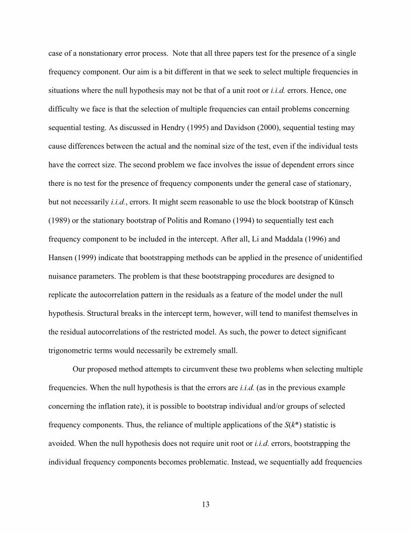
case of a nonstationary error process. Note that all three papers test for the presence of a single

frequency component. Our aim is a bit different in that we seek to select multiple frequencies in

situations where the null hypothesis may not be that of a unit root or i.i.d. errors. Hence, one

difficulty we face is that the selection of multiple frequencies can entail problems concerning

sequential testing. As discussed in Hendry (1995) and Davidson (2000), sequential testing may

cause differences between the actual and the nominal size of the test, even if the individual tests

have the correct size. The second problem we face involves the issue of dependent errors since

there is no test for the presence of frequency components under the general case of stationary,

but not necessarily i.i.d., errors. It might seem reasonable to use the block bootstrap of Künsch

(1989) or the stationary bootstrap of Politis and Romano (1994) to sequentially test each

frequency component to be included in the intercept. After all, Li and Maddala (1996) and

Hansen (1999) indicate that bootstrapping methods can be applied in the presence of unidentified

nuisance parameters. The problem is that these bootstrapping procedures are designed to

replicate the autocorrelation pattern in the residuals as a feature of the model under the null

hypothesis. Structural breaks in the intercept term, however, will tend to manifest themselves in

the residual autocorrelations of the restricted model. As such, the power to detect significant

trigonometric terms would necessarily be extremely small.

Our proposed method attempts to circumvent these two problems when selecting multiple

frequencies. When the null hypothesis is that the errors are i.i.d. (as in the previous example

concerning the inflation rate), it is possible to bootstrap individual and/or groups of selected

frequency components. Thus, the reliance of multiple applications of the S(k*) statistic is

avoided. When the null hypothesis does not require unit root or i.i.d. errors, bootstrapping the

individual frequency components becomes problematic. Instead, we sequentially add frequencies

14

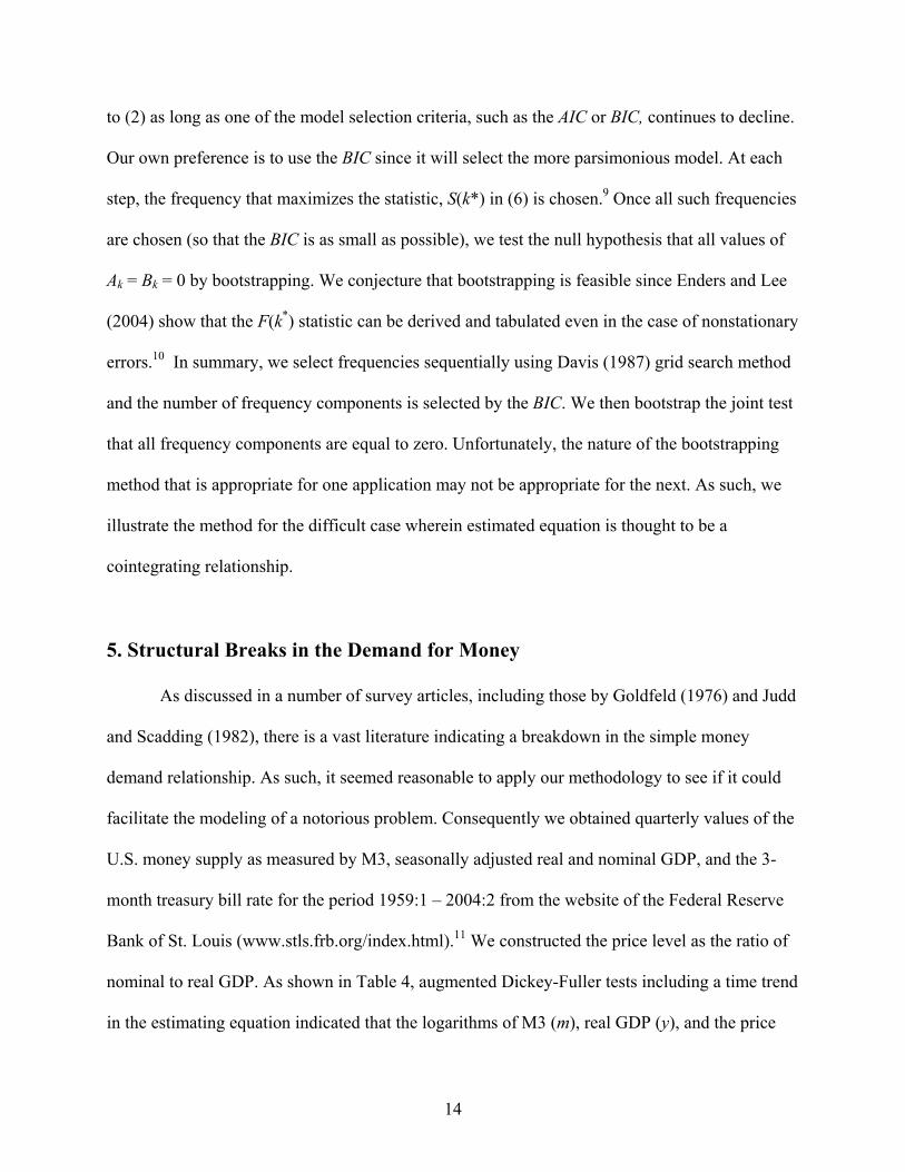
to (2) as long as one of the model selection criteria, such as the AIC or BIC, continues to decline.

Our own preference is to use the BIC since it will select the more parsimonious model. At each

step, the frequency that maximizes the statistic, S(k*) in (6) is chosen.9 Once all such frequencies

are chosen (so that the BIC is as small as possible), we test the null hypothesis that all values of

Ak = Bk = 0 by bootstrapping. We conjecture that bootstrapping is feasible since Enders and Lee

(2004) show that the F(k*) statistic can be derived and tabulated even in the case of nonstationary

errors.10 In summary, we select frequencies sequentially using Davis (1987) grid search method

and the number of frequency components is selected by the BIC. We then bootstrap the joint test

that all frequency components are equal to zero. Unfortunately, the nature of the bootstrapping

method that is appropriate for one application may not be appropriate for the next. As such, we

illustrate the method for the difficult case wherein estimated equation is thought to be a

cointegrating relationship.

5. Structural Breaks in the Demand for Money

As discussed in a number of survey articles, including those by Goldfeld (1976) and Judd

and Scadding (1982), there is a vast literature indicating a breakdown in the simple money

demand relationship. As such, it seemed reasonable to apply our methodology to see if it could

facilitate the modeling of a notorious problem. Consequently we obtained quarterly values of the

U.S. money supply as measured by M3, seasonally adjusted real and nominal GDP, and the 3-

month treasury bill rate for the period 1959:1 – 2004:2 from the website of the Federal Reserve

Bank of St. Louis (www.stls.frb.org/index.html).11 We constructed the price level as the ratio of

nominal to real GDP. As shown in Table 4, augmented Dickey-Fuller tests including a time trend

in the estimating equation indicated that the logarithms of M3 (m), real GDP (y), and the price

15

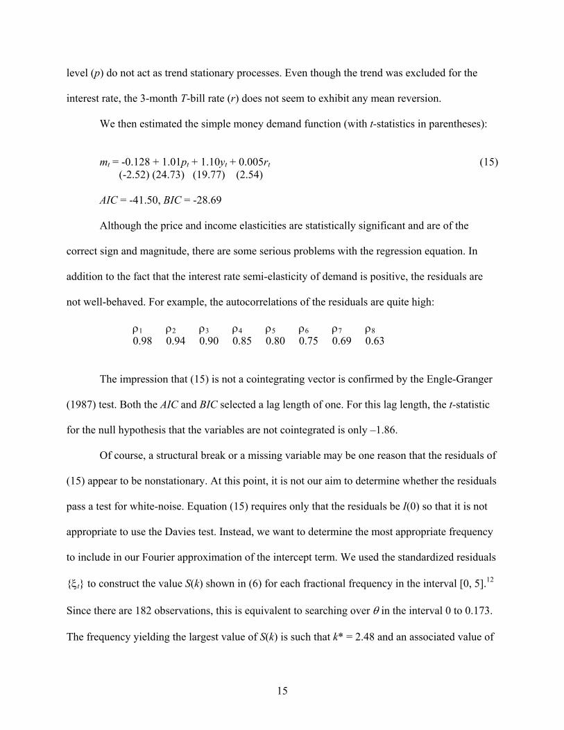
level (p) do not act as trend stationary processes. Even though the trend was excluded for the

interest rate, the 3-month T-bill rate (r) does not seem to exhibit any mean reversion.

We then estimated the simple money demand function (with t-statistics in parentheses):

mt = -0.128 + 1.01pt + 1.10yt + 0.005rt (15)

(-2.52) (24.73) (19.77) (2.54) AIC = -41.50, BIC = -28.69 Although the price and income elasticities are statistically significant and are of the

correct sign and magnitude, there are some serious problems with the regression equation. In

addition to the fact that the interest rate semi-elasticity of demand is positive, the residuals are

not well-behaved. For example, the autocorrelations of the residuals are quite high:

ρ1 ρ2 ρ3 ρ4 ρ5 ρ6 ρ7 ρ8 0.98 0.94 0.90 0.85 0.80 0.75 0.69 0.63

The impression that (15) is not a cointegrating vector is confirmed by the Engle-Granger

(1987) test. Both the AIC and BIC selected a lag length of one. For this lag length, the t-statistic

for the null hypothesis that the variables are not cointegrated is only –1.86.

Of course, a structural break or a missing variable may be one reason that the residuals of

(15) appear to be nonstationary. At this point, it is not our aim to determine whether the residuals

pass a test for white-noise. Equation (15) requires only that the residuals be I(0) so that it is not

appropriate to use the Davies test. Instead, we want to determine the most appropriate frequency

to include in our Fourier approximation of the intercept term. We used the standardized residuals

{ξt} to construct the value S(k) shown in (6) for each fractional frequency in the interval [0, 5].12

Since there are 182 observations, this is equivalent to searching over θ in the interval 0 to 0.173.

The frequency yielding the largest value of S(k) is such that k* = 2.48 and an associated value of

16

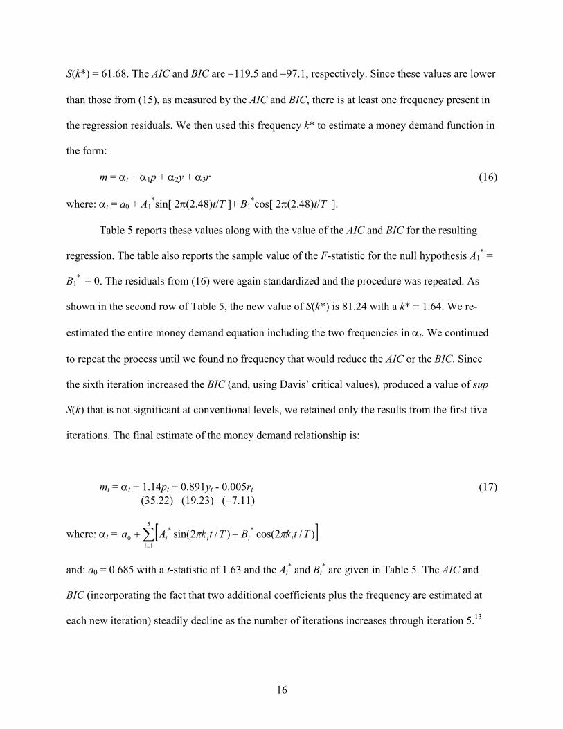
S(k*) = 61.68. The AIC and BIC are −119.5 and −97.1, respectively. Since these values are lower

than those from (15), as measured by the AIC and BIC, there is at least one frequency present in

the regression residuals. We then used this frequency k* to estimate a money demand function in

the form:

m = αt + α1p + α2y + α3r (16)

where: αt = a0 + A1*sin[ 2π(2.48)t/T ]+ B1

*cos[ 2π(2.48)t/T ].

Table 5 reports these values along with the value of the AIC and BIC for the resulting

regression. The table also reports the sample value of the F-statistic for the null hypothesis A1* =

B1* = 0. The residuals from (16) were again standardized and the procedure was repeated. As

shown in the second row of Table 5, the new value of S(k*) is 81.24 with a k* = 1.64. We re-

estimated the entire money demand equation including the two frequencies in αt. We continued

to repeat the process until we found no frequency that would reduce the AIC or the BIC. Since

the sixth iteration increased the BIC (and, using Davis’ critical values), produced a value of sup

S(k) that is not significant at conventional levels, we retained only the results from the first five

iterations. The final estimate of the money demand relationship is:

mt = αt + 1.14pt + 0.891yt - 0.005rt (17)

(35.22) (19.23) (−7.11)

where: αt = [ ]∑=

++5

1

**0 )/2cos()/2sin(

iiiii TtkBTtkAa ππ

and: a0 = 0.685 with a t-statistic of 1.63 and the Ai

* and Bi* are given in Table 5. The AIC and

BIC (incorporating the fact that two additional coefficients plus the frequency are estimated at

each new iteration) steadily decline as the number of iterations increases through iteration 5.13

17

The final model fits the data quite well. As in (15), the price and income elasticities are of

the correct magnitude. However, the interest rate semi-elasticity of demand for money now has

the correct sign with a magnitude that is 7.1 times its standard error. The residuals are well-

behaved. The last column of the table shows the t-statistic for the Engle-Granger (1987)

cointegration test using the frequency components through iteration i. Notice that incorporating

these frequency components enables us to reject a null hypothesis of no cointegration.14 Figure 4

provides a visual representation of αt. The striking impression is that the demand for money

generally rose from 1959 through 1987. At this point, the demand for money suddenly declined.

The decline continued through 1995 and then resumed its upward movement.

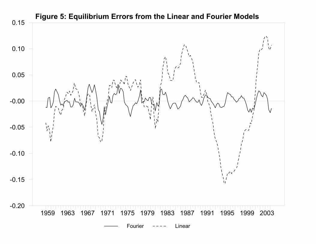
Another way to make the same point is to compare residuals (i.e., the ‘equilibrium

errors’) from (15) and (17). As shown in Figure 5, the residuals from the Fourier model are only

slightly better than those of the linear model over the first half of the sample period. The fact that

the residuals of the linear model become highly persistent beginning in 1982 is consistent with

the notion that (15) is not a cointegrating relationship. In contrast, the residuals of the Fourier

model are not highly persistent and behave similarly throughout the entire sample period.

5.1 The Bootstrap

Supporting evidence for the significance of the selected trigonometric series can be

gathered by testing the null hypothesis δ = 0 in the following cointegrated system:

yt = xtβ + dtδ + et (18)

xt = xt-1 + µt (19)

where: xt is a vector of I(1) exogenous variables, dt is the vector containing the relevant sine and

cosine terms in the Fourier expansion of the constant, et is the vector of residuals from the

cointegrating regression and µt is a vector of I(0) error terms. Small sample properties of

18

inference on δ can at times be unsatisfactory (Li and Maddala, 1997) and bootstrapping methods

have been proposed to improve such inference.

Generating bootstrap critical values for inference in cointegrated equations is, however,

not straightforward. Bootstrapping the significance of the test statistic for δ = 0 in equation (18)

using only the empirical distribution of error process et is inappropriate since it ignores the

possibility that the errors may be autocorrelated and that the regressors in xt might be

endogenous in the sense that that the elements of µt are correlated with et. Li and Maddala (1997)

and Psaradakis (2001) introduced bootstrap procedures to be applied in this framework.

Although they do not provide a formal proof, they present simulation evidence to establish that

the bootstrap procedure introduced here achieves significantly improved small sample

inference.15

A bootstrapping procedure allowing for autocorrelated residuals and endogeneity of xt is

performed according to the following steps (Psaradakis, 2001):

1. We estimate (18) and (19) using fully-modified least squares under the null hypothesis δ = 0 to obtain a consistent estimate of β. The estimated model yields the residual estimates: t̂e and ˆ tµ . 2. We draw bootstrap replications for the matrix of residuals *ˆ ˆ ˆ( , )t t te ′=µ µ . To account for all possible autocorrelations and crosscorrelations, we estimate *ˆ tµ as the VAR(p) system:

* *0

1

ˆ ˆp

t i t ti

γ γ=

= + +∑µ µ ε (20)

Resampling the estimated residuals from (20) yields the bootstrap estimates of *ˆ tµ . 3. These bootstrap estimates are then used to construct the resampled values of xt and yt . Using the bootstrapped data, the model in (18) may be re-estimated and by repetition of this procedure the empirical distribution of the LR statistic for the null hypothesis δ = 0 may be built up and a prob-value derived.

19

When we preformed this procedure using the five frequency components reported in

Table 5, we obtained a sample statistic with a prob-value of 0.000. As such, there is strong

support for the claim that (17) forms a cointegrating relationship.

5.2 The error-correction model In the presence of αt, the four variables appear to form a cointegrating relationship; as

such, there exists an error-correction representation such that m, y, p and r adjust to the

discrepancy from the long-run equilibrium relationship. However, unlike a traditional error-

correction model, adjustment will be nonlinear since the constant in the cointegrating vector is a

function of time. As such, we estimated the following error-correcting model using the residuals

from (17) as the error-correction term. Consider:

∆mt = -0.207ect-1 + A11(L)∆mt-1 + A12(L)∆pt-1 + A13(L)∆yt-1 + A14(L)∆rt-1 (21) (-5.94) (0.000) (0.248) (0.062) (0.141)

∆pt = 0.054ect-1 + A21(L)∆mt-1 + A22(L)∆pt-1 + A23(L)∆yt-1 + A24(L)∆rt-1 (22) (3.02) (0.742) (0.000) (0.306) (0.254)

∆yt = 0.091ect-1 + A31(L)∆mt-1 + A32(L)∆pt-1 + A33(L)∆yt-1 + A34(L)∆rt-1 (23) (1.75) (0.462) (0.817) (0.011) (0.0030)

∆rt = 0.676ect-1 + A41(L)∆mt-1 + A42(L)∆pt-1 + A43(L)∆yt-1 + A44(L)∆rt-1 (24) (1.45) (1.56) (0.001) (0.000) (0.000)

where: ect-1 = error-correction term (as measured by the residual from (17), Aij(L) = third-order

polynomials in the lag operator L, parenthesis contain the t-statistic for the null hypothesis that

the coefficient on the error-correction term is zero or the F-statistic for the null-hypothesis that

all coefficients in Aij(L) = 0, and constant terms in the intercepts are not reported.

20

Note that the money supply contracts and the price level increases in response to the

previous period’s deviation from the long-run equilibrium. However, income and the interest rate

appear to be weakly exogenous.

5.3 The restricted model One possible concern about the system given by (21) − (24) is money and the price level

appear to be jointly determined endogenous variables. Moreover, income is weakly exogenous

at the 5% significance level but not at the 10% level. With several jointly endogenous variables,

the single-equation approach to examining a cointegrating relationship may be inappropriate

unless a fully modified least squares procedure, such as that developed by Phillips and Hansen

(1990), is used. For our purposes, it is convenient that the income and price elasticities of the

money demand function are very close to unity. As such, it is possible for us to simply

investigate the restricted money demand equation:

mpt = -0.425 + 0.005rt (25) (-31.50) (2.53) AIC = -26.63 BIC = -29.84

where: mpt = the logarithm of real money balanced divided by real GDP (i.e., mt – pt – yt).

In (25), the interest rate is weakly exogenous and the money supply, price level and

income level all appear in the left-hand-side variable mt – pt – yt. This regression suffered the

same problems as the unconstrained form of the money demand function. After applying our

methodology to the constrained money demand function we obtained:

mpt = α(t) - 0.003rt (26) (-3.82) AIC = -550.03 BIC = -499.57

21

and αt = has the same form as (17).

The time path of αt (not shown) is virtually identical to that shown in Figure 4. The error-

correction model using the constrained form of the money-demand function is:

∆mpt = -0.312ect-1 + A11(L)∆mpt-1 + A12(L)∆rt-1 (27) (-6.98) (0.000) (0.000) ∆rt = 2.75ect-1 + A21(L)∆mpt-1 + A22(L)∆rt-1 (28) (0.677) (0.098) (0.000)

where: ect-1 = error-correction term (as measured by the residual from (23), Aij(L) = third-order

polynomials in the lag operator L, parenthesis contain the t-statistic for the null hypothesis that

the coefficient on the error-correction term is zero or the F-statistic for the null-hypothesis that

all coefficients in Aij(L) = 0, and intercepts are not reported.

5.4 Integer Frequencies In order to illustrate the use of integer frequencies and to compare the approximation to

that using continuous frequencies, we re-estimated the money demand function using discrete

frequencies in the expanded interval [ 1, 8 ] so that θ ranges from 0.0345 to 0.241 in steps of

0.0345.

The results from estimating the money demand function with integer frequencies are

shown in Table 6. The form is the same as that in (17) except that discrete frequencies 1, 2, 3, 4,

5 and 6 are used in the approximation for αt. The bootstrap methodology need not be modified in

any important way when using integer frequencies. As a group, these six integer frequencies are

statistically significant at conventional levels. Although the fit (as measured by the AIC and BIC)

is not as good as that using continuous frequencies, the Engle-Granger test strongly suggests that

22

the residuals are stationary. The time-path of αt using discrete frequencies (not shown) is nearly

identical to that obtained using fractional frequencies.

5.5 Missing Variables As suggested by Clements and Hendry (1998), a specification error resulting from an

omitted variable can manifest itself in parameter instability. One major advantage of ‘backing-

out’ the form of αt is that it might help to suggest the missing variable responsible for parameter

instability. Certainly, if a variable has the same time path as αt, including it as a regressor would

capture any instability in the intercept. In terms of our money demand analysis, the inclusion of a

variable having the time profile exhibited in Figure 4 might suggest the form of the missing

money. To demonstrate the point, we included a time trend in the demand for money function

such that:

αt = a0 + b0 t + (a1 + b1 t)d1 + (a2 + b2 t)d2 (29)

where: d1 = 1 for 1982:2 < t ≤ 1995:2 and 0 otherwise

d2 = 1 for t > 1995:2 and 0 otherwise

Thus, instead of using our Fourier approximation, we represent αt by a linear trend with

breaks in the intercept and slope coefficients occurring at the time periods suggested by Figure 4.

The estimated money demand function is:

mt = αt + 0.807pt + 0.571yt - 0.004rt (30) (18.62) (6.16) (-3.89) αt = 2.49 + 0.008t + ( 1.65 - 0.014t )d1 + (-1.04 + 0.004t )d2 (3.79) (6.57) (21.14) (-22.34) (-15.54) (9.45)

AIC = -476.71 BIC = -447.88

The Engle-Granger test indicates that the residuals from (30) are stationary: with four

lags in the augmented form of the test, the t-statistic on the lagged level of the residuals is –5.07.

23

As measured by the AIC and BIC, this form of the money demand function does not fit the data

quite as well as those using the Fourier approximation. Moreover, the price and income

elasticities have been shifted downward. One reason for the superior fit of the Fourier model

might simply be the fact that breaks in the time trend are actually smooth rather than sharp.

Although the Fourier approximations have better overall properties than (30), we used a

trend-line containing two breaks for illustrative purposes only. The point is that a Fourier

approximation can be used to ‘back-out’ the time-varying intercept. As such, the visual depiction

of the time-varying intercept can be suggestive of a missing explanatory variable. Of course, in

addition to a broken trend-line, there are other candidate variables. Figure 4 suggests that the

large decline in wealth following Black Monday in October of 1987 might have been responsible

for the decline in money demand. As stock prices recovered, the demand for M3 seemed to have

resumed its upward trend. There does not seem to be enough data to determine whether the stock

market decline following the events of 9 September 2001 had a similar effect on money demand.

6. Conclusion

In the paper, we developed a simple method that can be used to test for a time-varying

intercept and to approximate its form. The method uses a Fourier approximation to capture any

variation in the intercept term. As such, the issue becomes one of deciding which frequencies to

include in the approximation. The test for a structural break works nearly as well as the Andrews

and Ploberger (1994) optimal test if there is one break and can have substantially more power in

the presence of multiple breaks. Perhaps, the most important point is that successive applications

of the test can be used to ‘back-out” the form of the time-varying intercept.

A number of diagnostic tests indicate that a linear autoregressive model of the U.S.

inflation rate (as measured by the CPI) is inappropriate. It was shown that our methodology is

24

capable of ‘backing-out’ the form of the nonlinearity. We also explored the nature of the

approximation using an extended example concerning the demand for M3. Using quarterly U.S.

data over the 1959:1 – 2004:2 period, we confirmed the standard result that the demand for

money is not a stable linear function of real income, the price level and a short-term interest rate.

The incorporation of the time-varying intercept resulting from the Fourier approximation appears

to result in a stable money demand function. Moreover, the magnitudes of the coefficients are

quite plausible and all are significant at conventional levels. The form of the intercept term

suggests a fairly steady growth rate in the demand for M3 until late-1987. At that point, there

was a sharp and sustained drop in demand. Money demand continued to decline until mid-1995

and then resumed its upward trend. The implied error-correction model appears to be reasonable

in that money and the price level (but neither income nor the interest rate) adjust to eliminate any

discrepancy in money demand.

There are a number of important limitations of the methodology. First, in a regression

analysis, a structural break may affect the slope coefficients as well as the intercept. Our

methodology forces the effects of the structural change to manifest itself only in the intercept

term. A related point is that the alternative hypothesis in the test is that the residuals are not

white-noise. It is quite possible that the methodology captures any number of departures from

white-noise and places them in the intercept term. Third, we have not addressed the issue of out-

of-sample forecasting. Although the Fourier approximation has very good in-sample properties,

it is not clear how to extend the intercept term beyond the observed data. Our preference is to use

an average of the last few values of αt for out-of-sample forecasts. However, there are a number

of other possibilities that are equally plausible. Anyone who has read the paper to this point can

25

certainly add to the list of limitations. Nevertheless, we believe that the methodology explored in

this paper can be useful for modeling in the presence of structural change.

26

References

Andrews, Donald (1993), “Tests for parameter instability and structural change with unknown

Change Point,” Econometrica 61, 821 – 856.

Andrews, Donald and W. Ploberger (1994), “Optimal tests when a nuisance parameter is present

only under the alternative,” Econometrica 62, 1383 – 1414.

Bai, J. and P. Perron, 1998, “Estimating and testing linear models with multiple structural

changes,” Econometrica 66, 47 − 78.

Baillie, R. T., Han, Y.W. and Kwon, T. (2002), "Further long memory properties of inflationary

shocks," Southern Economic Journal 68, 496 – 510.

Becker, R., W. Enders, and S. Hurn, (2004), A general test for time dependence in parameters,

Journal of Applied Econometrics 19, 899 − 906.

Chow, Gregory (1960), “Tests of equality between sets of coefficients in two linear regressions,”

Economertica 28, 591 – 605.

Chow, Gregory (1984), “Random and changing coefficient models,” in Griliches, Z. and Michael

Intriligator, eds., Handbook of Econometrics, vol. II. (Elsevier: Amsterdam). pp. 1213 –

1245.

Clements, M.P. and Hendry D.H. (1998), Forecasting Economic Time Series. (MIT Press:

Cambridge).

Clements, M. and Mizon, G.E. (1991), “Empirical analysis of macroeconomic time series,”

European Economic Review 35, 887-932.

Davidson, James (2000), Econometric Theory, (Blackwell: Oxford).

Davies, Robert (1987), “Hypothesis testing when a nuisance parameter is present only under the

null hypothesis,” Biometrica 74, 33 - 43.

27

Enders, Walter and Junsoo Lee (2004), “Testing for a unit root with a nonlinear fourier

function,” mimeo. Available at: www.cba.ua.edu/~wenders.

Engle, Robert F. and C. W. J. Granger (1987), “Cointegration and error correction:

representation, estimation and testing,” Econometrica 55, 251 - 276.

Farley, John and Melvin Hinich (1975), “Some comparisons of tests for a shift in the slopes of a

multivariate linear time series model,” Journal of Econometrics 3, 279 – 318.

Farley, John and Melvin Hinich (1970), “A test for a shifting slope coefficient in a linear model,”

Journal of the American Statistical Association 65, 1320 – 1329.

Gallant, Ronald (1984), “The Fourier flexible form,” American Journal of Agricultural

Economics 66, 204 − 208.

Gallant, Ronald and G. Souza (1991), “On the asymptotic normality of Fourier flexible form

estimates,” Journal of Econometrics 50, 329 − 353.

Goldfeld, S. M. (1976)’ “The case of the missing money,” Brookings Papers on Economic

Activity 3, 683 – 730.

Hansen, Bruce (1992), “Tests for parameter instability in regressions with I(1) processes,”

Journal of Business and Economic Statistics 10, 321 – 335.

Hansen, Bruce (1999), “Testing for linearity” Journal of Economic Surveys 13, 551-576.

Harvey, Andrew (1989), Forecasting, Structural Time Series Models and the Kalman Filter.

(Cambridge University Press: Cambridge).

Hausman, J. A. (1978), “Specification tests in econometrics,” Econometrica 46, 1251 – 1272.

Hendry, David (1995), Dynamic Econometrics, (Oxford University Press: Oxford).

Judd, J. and J. Scadding (1982), “The search for a stable money demand function: A survey of

the post-1973 literature,” Journal of Economic Literature 20, 993 – 1023.

28

Künsch, H.R. (1989), “The jackknife and the bootstrap for general stationary observations,” The

Annals of Statistics 17, 1217-1241.

Leybourne, S., Newbold, P. and Vougas, D. (1998) “Unit roots and smooth transitions”, Journal

of Time Series Analysis 19, 83-97.

Li, H. and Maddala, G.S. (1996), “Bootstrapping time-series models,” Econometric Reviews 15,

115-195.

Li H. and Maddala G.S. (1997), “Bootstrapping cointegrated regressions,” Journal of

Econometrics, 80, 297-318.

Lin, Chien-Fu Jeff and Timo Teräsvirta (1994), “Testing the constancy of regression parameters

against continuous structural change,” Journal of Econometrics 62, 211-228.

Phillips, Peter and Bruce Hansen (1990), “Statistical inference in instrumental variables

regression with I(1) processes,” Review of Economic Studies 57, 99 – 125.

Politis, D.N. and Romano J.P. (1994), “The stationary bootstrap,” Journal of the American

Statistical Association 89, 1303-1313.

Psaradakis Z. (2001), “On bootstrap inference in cointegrating regressions,” Economics Letters,

72, 1-10.

Ripatti, Antti and Saikonnen, Pentti (2001) “Vector autoregressive processes with nonlinear time

trends in cointegrating relations,” Macroeconomic Dynamics 5, 577-597.

Rosenberg, B. (1973), “A survey of stochastic parameter regression,” Annals of Economic and

Social Measurement 2, 381 – 398.

Tan, Hui Boon and Richard Ashley (1999), "An elementary method for detecting and modeling

regression parameter variation across frequencies with an application to testing the

permanent income hypothesis." Macroeconomic Dynamics 3, 69 – 83.

29

Table 1: Critical Values for the F* Test with i.i.d. errors

T = 50

T = 100

T = 250

T = 1000

Maximum Frequency = T/2

90%

5.81

6.37

7.17

8.53

95%

6.72

7.19

7.94

9.25

99% 8.87

9.09

9.72

10.95

Maximum Frequency = T/4

90%

4.95

5.61

6.44

7.80

95%

5.84

6.46

7.19

8.53

99%

8.08

8.31

8.92

10.21 Maximum Frequency = T/12

90%

3.54

4.27

5.19

6.69

95%

4.38

5.09

5.94

7.44

99%

6.27

6.95

7.65

9.17

30

Table 2: Power of the Andrews-Ploberger and Davies Tests with One Break

Andrews δ = 0 δ = 0.5 δ = 1 1% 0.008 0.115 0.652 5% 0.043 0.274 0.825 10% 0.094 0.399 0.896 Davies δ = 0 δ = 0.5 δ = 1 1% 0.007 0.105 0.585 5% 0.047 0.290 0.794 10% 0.096 0.409 0.891 Table 1: Reports size (δ = 0) and power statistics for Andrews and Davies test applied to the process in (11 and 12). Significance evaluated by means of bootstrap.

Table 3: Power of the Andrews-Ploberger and Davies Tests with Two Breaks

Andrews δ = 0 δ = 0.5 δ = 1 1% 0.008 0.026 0.103 5% 0.043 0.103 0.294 10% 0.094 0.185 0.443 Davies δ = 0 δ = 0.5 δ = 1 1% 0.007 0.074 0.444 5% 0.047 0.213 0.671 10% 0.096 0.335 0.772 Table 2: Reports size (δ = 0) and power statistics for Andrews and Davies test applied to the process in (14). Significance evaluated by means of bootstrap.

Table 4: Results of the Dickey-Fuller Tests

Variable Lags t-statistic ∆m 1 -1.20 ∆y 2 -3.03 ∆p 3 -1.62 ∆r 3 -1.67

Critical values for the Dickey-Fuller test are -3.99, -3.43 and -3.13 at the 1%, 5% and 10% significance levels, respectively. Since the test for the interest rate did not include a deterministic time trend, the appropriate critical values for the ∆r equation are -3.46, -2.88 and -2.57 at the 1%, 5% and 10% significance levels, respectively.

31

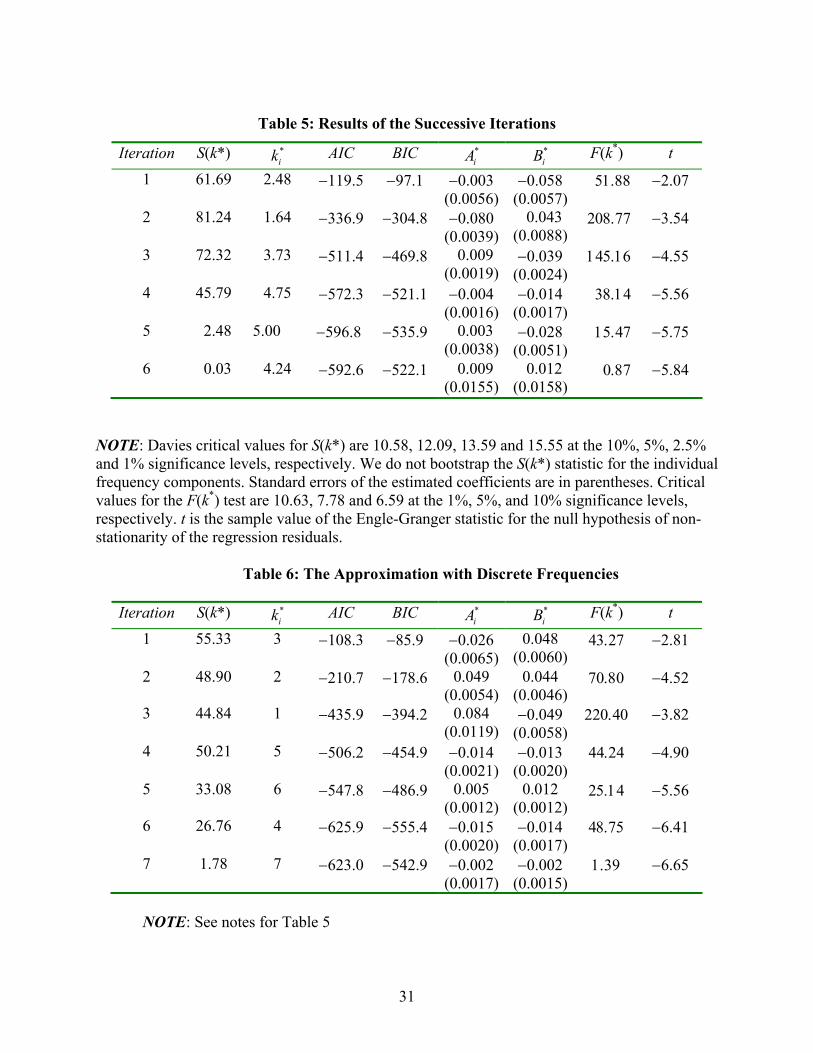
Table 5: Results of the Successive Iterations

Iteration S(k*) *ik AIC BIC *

iA *iB F(k*) t

1

61.69

2.48

−119.5

−97.1

−0.003 (0.0056)

−0.058 (0.0057)

51.88 −2.07

2

81.24

1.64

−336.9

−304.8

−0.080 (0.0039)

0.043 (0.0088)

208.77 −3.54

3

72.32

3.73

−511.4

−469.8

0.009 (0.0019)

−0.039 (0.0024)

145.16 −4.55

4

45.79

4.75

−572.3

−521.1

−0.004 (0.0016)

−0.014 (0.0017)

38.14 −5.56

5

2.48 5.00 −596.8 −535.9 0.003 (0.0038)

−0.028 (0.0051)

15.47 −5.75

6 0.03

4.24

−592.6

−522.1

0.009 (0.0155)

0.012 (0.0158)

0.87 −5.84

NOTE: Davies critical values for S(k*) are 10.58, 12.09, 13.59 and 15.55 at the 10%, 5%, 2.5% and 1% significance levels, respectively. We do not bootstrap the S(k*) statistic for the individual frequency components. Standard errors of the estimated coefficients are in parentheses. Critical values for the F(k*) test are 10.63, 7.78 and 6.59 at the 1%, 5%, and 10% significance levels, respectively. t is the sample value of the Engle-Granger statistic for the null hypothesis of non-stationarity of the regression residuals.

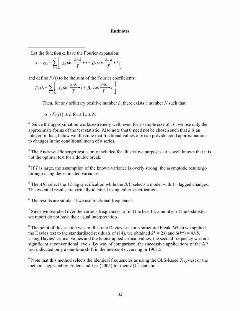
Table 6: The Approximation with Discrete Frequencies

Iteration S(k*) *ik AIC BIC *

iA *iB F(k*) t

1 55.33 3 −108.3 −85.9 −0.026 (0.0065)

0.048 (0.0060)

43.27 −2.81

2 48.90 2 −210.7 −178.6 0.049 (0.0054)

0.044 (0.0046)

70.80 −4.52

3 44.84 1 −435.9 −394.2 0.084 (0.0119)

−0.049 (0.0058)

220.40 −3.82

4 50.21 5 −506.2 −454.9 −0.014 (0.0021)

−0.013 (0.0020)

44.24 −4.90

5 33.08 6 −547.8 −486.9 0.005 (0.0012)

0.012 (0.0012)

25.14 −5.56

6 26.76 4 −625.9 −555.4 −0.015 (0.0020)

−0.014 (0.0017)

48.75 −6.41

7 1.78 7 −623.0 −542.9 −0.002 (0.0017)

−0.002 (0.0015)

1.39 −6.65

NOTE: See notes for Table 5

32

Endnotes

1 Let the function αt have the Fourier expansion:

sin cosk k0tk=1

2 k 2 k = + t + t A BT Tπ πα α

∞ • • ∑

and define Fs(t) to be the sum of the Fourier coefficients:

••∑ tT

k2 B + tT

k2 A = (t)F kk

s

=1ks

ππ cossin

Then, for any arbitrary positive number h, there exists a number N such that:

| αt - Fs(t) | ≤ h for all s ≥ N.

2 Since the approximation works extremely well, even for a sample size of 16, we use only the approximate forms of the test statistic. Also note that θ need not be chosen such that k is an integer; in fact, below we illustrate that fractional values of k can provide good approximations to changes in the conditional mean of a series. 3 The Andrews-Ploberger test is only included for illustrative purposes--it is well known that it is not the optimal test for a double break. 4 If T is large, the assumption of the known variance is overly strong; the asymptotic results go through using the estimated variance. 5 The AIC select the 12-lag specification while the BIC selects a model with 11-lagged changes. The essential results are virtually identical using either specification. 6 The results are similar if we use fractional frequencies. 7 Since we searched over the various frequencies to find the best fit, a number of the t-statistics we report do not have their usual interpretation. 8 The point of this section was to illustrate Davies test for a structural break. When we applied the Davies test to the standardized residuals of (14), we obtained k* = 2.0 and S(k*) = 4.95. Using Davies’ critical values and the bootstrapped critical values, the second frequency was not significant at conventional levels. By way of comparison, the successive applications of the AP test indicated only a one-time shift in the intercept occurring in 1967:5 9 Note that this method selects the identical frequencies as using the OLS-based Trig-test or the method suggested by Enders and Lee (2004) for their F(k*) statistic.

33

10 Note that the Enders and Lee (2004) critical values are not directly applicable to our study of the money demand function. Their critical values are derived from a univariate framework and not from a cointegrated system. Nevertheless, the fact that there is a distribution of the unit-root case suggests that there is a distribution for the case of cointegrated variables. 11 Almost identical results to those reported below hold if we use M2 instead of M3. 12 We used a maximum value of k = 5 since we wanted to consider only ‘low frequency’ changes in the intercept. Also note that we searched at intervals of 1/512. The results turn out to be similar if we use integer frequencies. 13 Also shown in Table 5 is the sample value of F(k*). It is interesting to note that these values of F(k*) exceed the critical values reported by Enders and Lee (2004) through iteration 5. 14 It is not our intention here to provide a new test for cointegration. Note that the critical values for the Engle-Granger test may depend on the inclusion of the frequency components. After all, the frequency components were chosen by means of a grid search so as to provide the component with the best fit. A proper cointegration test would bootstrap the critical of the Engle-Granger test statistic. However, that would take us far beyond the purpose of this paper. 15 To the best of our knowledge, no theoretical arguments are available yet, to establish whether this, or any other bootstrap procedure, generates consistent inference in the context of cointegrated regressions.

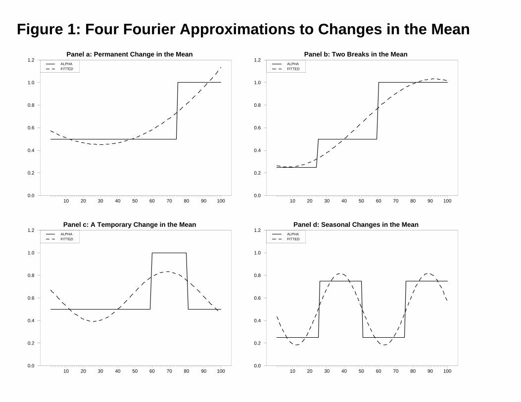
Figure 1: Four Fourier Approximations to Changes in the MeanPanel a: Permanent Change in the Mean

10 20 30 40 50 60 70 80 90 1000.0

0.2

0.4

0.6

0.8

1.0

1.2ALPHAFITTED

Panel c: A Temporary Change in the Mean

10 20 30 40 50 60 70 80 90 1000.0

0.2

0.4

0.6

0.8

1.0

1.2ALPHAFITTED

Panel b: Two Breaks in the Mean

10 20 30 40 50 60 70 80 90 1000.0

0.2

0.4

0.6

0.8

1.0

1.2ALPHAFITTED

Panel d: Seasonal Changes in the Mean

10 20 30 40 50 60 70 80 90 1000.0

0.2

0.4

0.6

0.8

1.0

1.2ALPHAFITTED

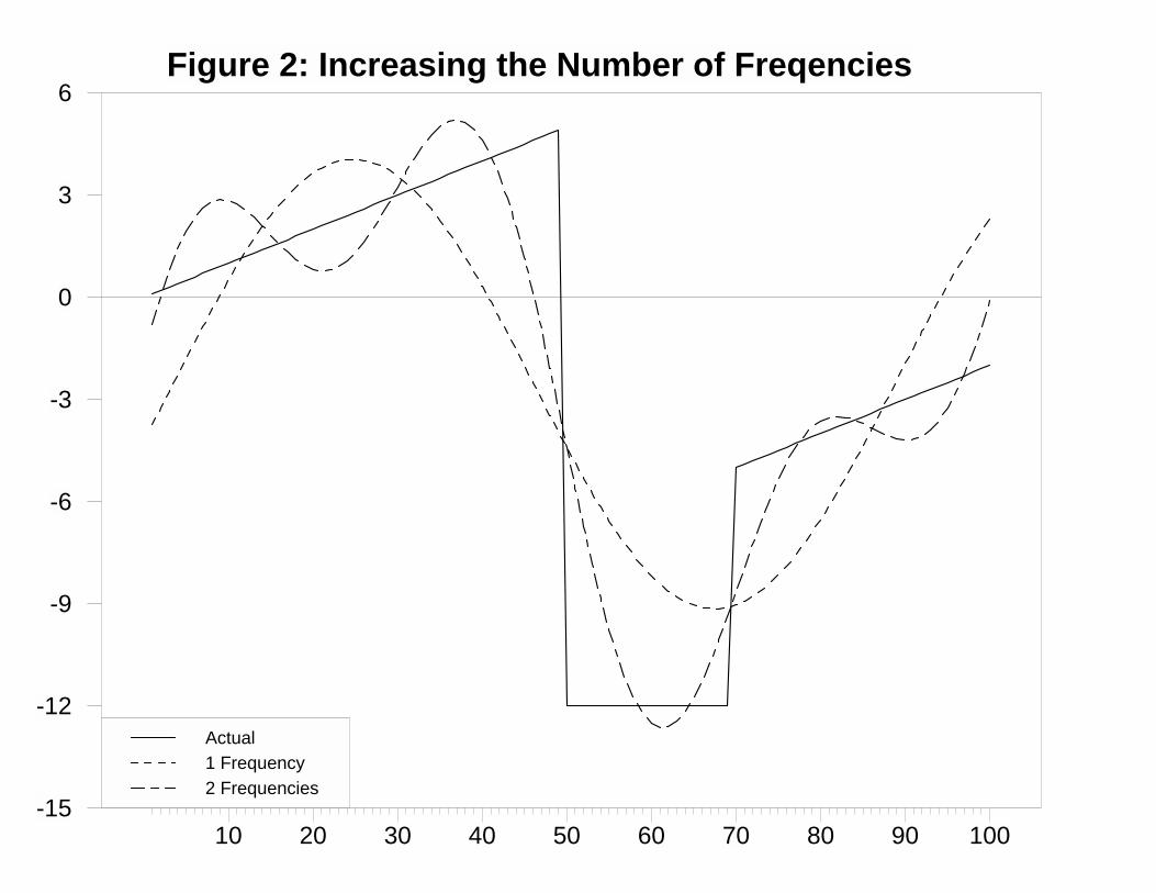
Figure 2: Increasing the Number of Freqencies

10 20 30 40 50 60 70 80 90 100-15

-12

-9

-6

-3

0

3

6

Actual1 Frequency2 Frequencies

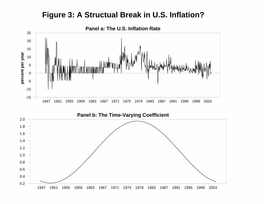
Figure 3: A Structual Break in U.S. Inflation?Panel a: The U.S. Inflation Rate

perc

ent p

er y

ear

1947 1951 1955 1959 1963 1967 1971 1975 1979 1983 1987 1991 1995 1999 2003-15

-10

-5

0

5

10

15

20

25

Panel b: The Time-Varying Coefficient

1947 1951 1955 1959 1963 1967 1971 1975 1979 1983 1987 1991 1995 1999 20030.2

0.4

0.6

0.8

1.0

1.2

1.4

1.6

1.8

2.0

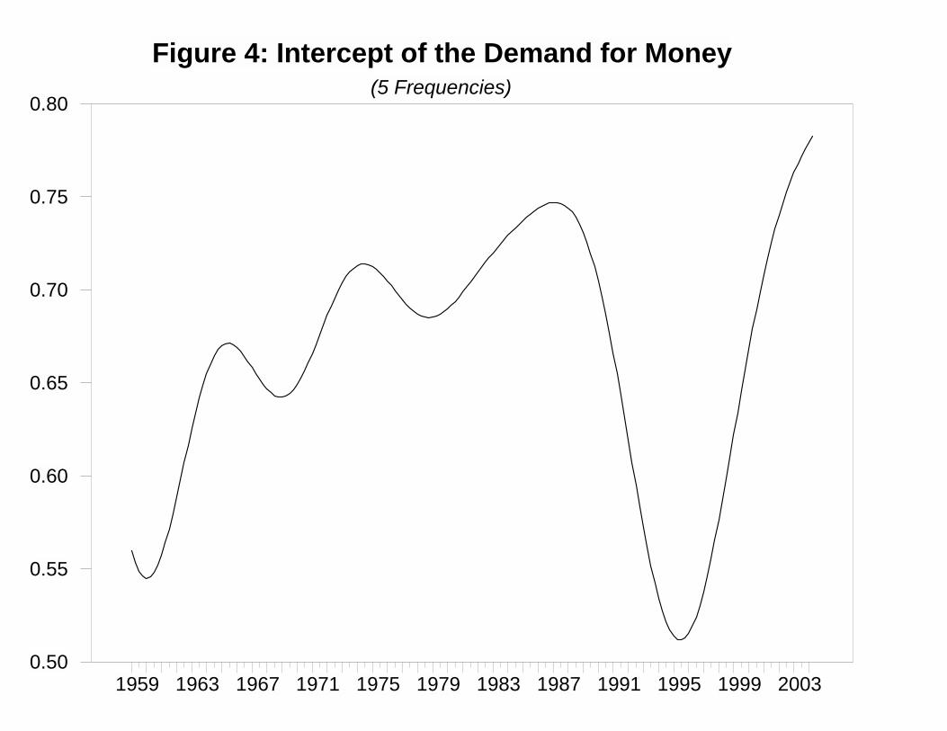
Figure 4: Intercept of the Demand for Money(5 Frequencies)

1959 1963 1967 1971 1975 1979 1983 1987 1991 1995 1999 20030.50

0.55

0.60

0.65

0.70

0.75

0.80

Fourier Linear

Figure 5: Equilibrium Errors from the Linear and Fourier Models

1959 1963 1967 1971 1975 1979 1983 1987 1991 1995 1999 2003-0.20

-0.15

-0.10

-0.05

-0.00

0.05

0.10

0.15