Coastal Engineering 58 (2011) 45–65

Contents lists available at ScienceDirect

Coastal Engineering

j ourna l homepage: www.e lsev ie r.com/ locate /coasta leng

Modeling hurricane waves and storm surge using integrally-coupled,scalable computations

J.C. Dietrich a,⁎, M. Zijlema b, J.J. Westerink a, L.H. Holthuijsen b, C. Dawson c, R.A. Luettich Jr. d, R.E. Jensen e,J.M. Smith e, G.S. Stelling b, G.W. Stone f

a Department of Civil Engineering and Geological Sciences, University of Notre Dame, 156 Fitzpatrick Hall, Notre Dame, IN 46556, United Statesb Faculty of Civil Engineering and Geosciences, Delft University of Technology, Stevinweg 1, 2628 CN, Delft, The Netherlandsc Institute for Computational Engineering and Sciences, University of Texas at Austin, 201 East 24 Street, Austin, TX 78712, United Statesd Institute of Marine Sciences, University of North Carolina at Chapel Hill, 3431 Arendell Street, Morehead City, NC 28557, United Statese Coastal and Hydraulics Laboratory, U.S. Army Engineer Research and Development Center, 3909 Halls Ferry Road, Vicksburg, MS 39180, United Statesf Coastal Studies Institute, Louisiana State University, Old Geology Building, Room 331, Baton Rouge, LA 70803, United States

⁎ Corresponding author. Tel.: +1 574 631 3864.E-mail addresses: dietrich.15@nd.edu (J.C. Dietrich),

(M. Zijlema), jjw@nd.edu (J.J. Westerink), l.h.holthuijsenclint@ices.utexas.edu (C. Dawson), rick_luettich@unc.edrobert.e.jensen@usace.army.mil (R.E. Jensen), jane.m.sm(J.M. Smith), g.s.stelling@tudelft.nl (G.S. Stelling), gagre

0378-3839/$ – see front matter © 2010 Elsevier B.V. Aldoi:10.1016/j.coastaleng.2010.08.001

a b s t r a c t

a r t i c l e i n f o

Article history:Received 26 March 2010Received in revised form 9 July 2010Accepted 9 August 2010

Keywords:ADCIRCSWANHurricanesWavesStorm surge

The unstructured-mesh SWAN spectral wave model and the ADCIRC shallow-water circulation model havebeen integrated into a tightly-coupled SWAN+ADCIRC model. The model components are applied to anidentical, unstructured mesh; share parallel computing infrastructure; and run sequentially in time. Windspeeds, water levels, currents and radiation stress gradients are vertex-based, and therefore can be passedthrough memory or cache to each model component. Parallel simulations based on domain decompositionutilize identical sub-meshes, and the communication is highly localized. Inter-model communication is intra-core, while intra-model communication is inter-core but is local and efficient because it is solely on adjacentsub-mesh edges. The resulting integrated SWAN+ADCIRC system is highly scalable and allows for localizedincreases in resolution without the complexity or cost of nested meshes or global interpolation betweenheterogeneous meshes. Hurricane waves and storm surge are validated for Hurricanes Katrina and Rita,demonstrating the importance of inclusion of the wave-circulation interactions, and efficient performance isdemonstrated to 3062 computational cores.

m.zijlema@tudelft.nl@tudelft.nl (L.H. Holthuijsen),u (R.A. Luettich),ith@usace.army.milg@lsu.edu (G.W. Stone).

l rights reserved.

© 2010 Elsevier B.V. All rights reserved.

1. Introduction

A broad energy spectrum exists in oceans, with wave periodsranging from seconds to months. Short waves, such as wind-drivenwaves and swell, have periods that range from 0.5 to 25 s. Longerwaves, such as seiches, tsunamis, storm surges and tides, have periodsthat range from minutes to months. These short and long waves arewell-separated in the energy spectrum and have well-defined spatialscales. This separation leads to distinct modeling approaches,depending on whether the associated scales can be resolved. Foroceanic scales, short-wave models cannot resolve spatially ortemporally the individual wind-driven waves or swell, and thusthey treat the wave field as an energy spectrum and apply theconservation of wave action density to account for wave–currentinteractions. Long-wave models apply forms of conservation of mass

and momentum, in two or three spatial dimensions, to resolve thecirculation associated with processes such as tsunamis, storm surgesor tides.

Although wind-driven waves and circulation are separated in thespectrum, they can interact. Water levels and currents affect thepropagation of waves and the location of wave-breaking zones. Wavetransformation generates radiation stress gradients that drive set-upand currents. Wind-driven waves affect the vertical momentummixing and bottom friction, which in turn affect the circulation.Waterlevels can be increased by 5–20% in regions across a broad continentalshelf, and by asmuch as 35% in regions of steep slope (Funakoshi et al.,2008; Dietrich et al., 2010). Thus, in many coastal applications, wavesand circulation processes should be coupled.

Wave and circulation models have been limited by their spectral,spatial and temporal resolution. This limitation can be overcome bynesting structured meshes, to enhance resolution in specific regionsby employing meshes with progressively finer scales. In a waveapplication, nesting also allows the use of models with differentphysics and numerics. Relatively fine nearshore wave models, such asSTWAVE and SWAN, can be nested inside relatively coarse deep-water wave models, such as WAM and WaveWatch III (WAMDIGroup, 1988; Komen et al., 1994; Booij et al., 1999; Smith et al., 2001;

Fig. 1. Schematic of parallel communication between models and cores. Dashed lines indicate communication for all vertices within a sub-mesh, and are inter-model and intra-core.Solid lines indicate communication for the edge-layer-based nodes between sub-meshes, and are intra-model and inter-core.

Fig. 2. ADCIRC SL15 model domain with bathymetry (m).

46 J.C. Dietrich et al. / Coastal Engineering 58 (2011) 45–65

Thompson et al., 2004; Gunther, 2005; Tolman, 2009). The nearshorewave models may not be efficient if applied to large domains, and thedeep-water wave models may not contain the necessary physics orresolution for nearshorewave simulation. Until recently, wavemodelsrequired nesting in order to vary resolution from basin to shelf tonearshore applications. These structured wave models can be coupledto structured circulation models that run on the same nested meshes(Kim et al., 2008).

Unstructured circulation models have emerged to providelocalized resolution of gradients in geometry, bathymetry/topogra-phy, and flow processes. Resolution varies over a range of scaleswithin the same mesh from deep water to the continental shelf tothe channels, marshes and floodplains near shore (Westerink et al.,2008). Unstructured meshes allow for localized resolution wheresolution gradients are large and correspondingly coarser resolutionwhere solution gradients are small, thus minimizing the computa-tional cost relative to structured meshes with similar minimummesh spacings.

The coupling of wave and circulation models has been imple-mented typically with heterogeneous meshes. A coupling applicationmay have one unstructured circulation mesh and several structuredwave meshes, and the models may pass information via external files(Funakoshi et al., 2008; Dietrich et al., 2010; Weaver and Slinn, 2004;Ebersole et al., 2007; Chen et al., 2008; Pandoe and Edge, 2008; Bunyaet al., 2010). This ‘loose’ coupling is disadvantageous because itrequires intra-model interpolation at the boundaries of the nested,structured wave meshes and inter-model interpolation between thewave and circulation meshes. This interpolation creates problemswith respect to both accuracy and efficiency. Overlapping nested oradjacent wave meshes often have different solutions, and inter-meshinterpolation can smooth or enhance the integrated wave forcing.Furthermore, even if a component model is locally conservative, itsinterpolated solution will not necessarily be conservative. Finally,inter-model interpolation must be performed at all vertices of themeshes. This interpolation is problematic in a parallel computingenvironment, where the communication between sub-meshes isinter-model and semi-global. The sub-meshes must communicate onan area basis (i.e., the information at all vertices on a sub-mesh must

be shared). Global communication is costly and can prevent modelsfrom being scalable in high-performance computing environments.

An emerging practice is to couple models through a genericframework, such as the Earth System Modeling Framework (ESMF)(Hill et al., 2004; Collins et al., 2005), the Open Modeling Interface(OpenMI) Environment (Moore and Tindall, 2005; Gregersen et al.,2005) or the Modeling Coupling Toolkit (MCT) (Warner et al., 2008).These frameworks manage when and how the individual models arerun, interpolate information between models if necessary, and maketransparent the coupling to developers and users. However, theseframeworks do not eliminate the fundamental problems of couplingwhen using heterogeneous meshes. Boundary conditions must beinterpolated between nested, structured wave meshes, and waterlevels, currents and wave properties must be interpolated between

Fig. 3. ADCIRC SL15 bathymetry and topography (m), relative to NAVD88 (2004.65), for southern Louisiana.

47J.C. Dietrich et al. / Coastal Engineering 58 (2011) 45–65

the unstructured circulation and structured wave meshes. Thisinterpolation is costly, destroys the scalability of the coupled model,and thus limits the resolution that can be employed and thecorresponding physics that can be simulated.

The recent introduction of unstructured wave models makesnesting unnecessary. Resolution can be enhanced nearshore andrelaxed in deep water, allowing the model to simulate efficiently thewave evolution. SWAN has been used extensively to simulate wavesin shallow water (Booij et al., 1999; Ris et al., 1999; Gorman andNeilson, 1999; Rogers et al., 2003), and it has been converted recentlyto run on unstructured meshes (Zijlema et al., 2010). This version ofSWAN employs the unstructured-mesh analog to the solutiontechnique from the structured version. It retains the physics andnumerics of SWAN, but it runs on unstructured meshes, and it is bothaccurate and efficient in the nearshore and in deep water.

In this paper, we describe a ‘tight’ coupling of the SWAN wavemodel and the ADCIRC circulation model. SWAN and ADCIRC are runon the same unstructured mesh. This identical, homogeneous mesh

Fig. 4. ADCIRC SL15 mesh resoluti

allows the physics of wave-circulation interactions to be resolvedcorrectly in both models. The unstructured mesh can be applied on alarge domain to follow seamlessly all energy from deep to shallowwater. There is no nesting or overlapping of structured wave meshes,and there is no inter-model interpolation. Variables and forces resideat identical, vertex-based locations. Information can be passedwithout interpolation, thus reducing significantly the communicationcosts.

In parallel computing applications, identical sub-meshes andcommunication infrastructure are used for both SWAN and ADCIRC,which run as the same program on the same computational core. Allinter-model communication on a sub-mesh is done through localmemory or cache. Communication between sub-meshes is intra-model. Information is passed only to the edges of neighboring sub-meshes, and thus the coupled model does not require globalcommunication over areas. Domain decomposition places neighbor-ing sub-meshes on neighboring cores, so communication costs areminimized. The coupled model is highly scalable and integrates

on (m) in southern Louisiana.

Fig. 5. Example of the METIS domain decomposition of the ADCIRC SL15 mesh on 1014 computational cores. Colors indicate local sub-meshes and shared boundary layers.

48 J.C. Dietrich et al. / Coastal Engineering 58 (2011) 45–65

seamlessly the physics and numerics from ocean to shelf to floodplain.Large domains and high levels of local resolution can be employed forboth models, allowing the accurate depiction of the generation,propagation and dissipation of waves and surge. The resulting SWAN+ADCIRC model is suited ideally to simulate waves and circulationand their propagation from deep water to complicated nearshoresystems.

In the sections that follow, the component SWAN and ADCIRCmodels are described, and the mechanics of their tight coupling isintroduced. The coupled model is then validated through itsapplication to hindcasts of Hurricanes Katrina and Rita. Finally, abenchmarking study shows SWAN+ADCIRC is highly scalable.

2. Methods

2.1. SWAN model

SWAN predicts the evolution in geographical space⇀x and time t ofthe wave action density spectrum N(→x,t,σ,θ), with σ the relative

Table 1Geographic location by type and number shown in Figs. 6 and 7.

Rivers and channels1 Calcasieu Shipping Channel2 Atchafalaya River3 Mississippi River4 Southwest Pass

Bays, lakes and sounds5 Sabine Lake6 Calcasieu Lake7 White Lake8 Vermilion Bay9 Terrebonne Bay10 Timbalier Bay11 Lake Pontchartrain12 Lake Borgne13 Gulf of Mexico

Islands14 Grand Isle15 Chandeleur Islands

Places16 Galveston, TX17 Tiger and Trinity Shoals18 New Orleans, LA

frequency and θ the wave direction, as governed by the action balanceequation (Booij et al., 1999):

∂N∂t + ∇⇀x⋅ ⇀cg + ⇀U

� �N

h i+

∂cθN∂θ +

∂cσN∂σ =

Stotσ

: ð1Þ

The terms on the left-hand side represent, respectively, the changeof wave action in time, the propagation of wave action in ⇀x-space(with ∇⇀x the gradient operator in geographic space, ⇀cg the wavegroup velocity and ⇀U the ambient current vector), depth- and current-induced refraction and approximate diffraction (with propagationvelocity or turning rate cθ), and the shifting of σ due to variations inmean current and depth (with propagation velocity or shifting ratecσ). The source term, Stot, represents wave growth by wind; action lostdue to whitecapping, surf breaking and bottom friction; and actionexchanged between spectral components in deep and shallow waterdue to nonlinear effects. The associated SWAN parameterizations aregiven by Booij et al. (1999), with all subsequent modifications as

Fig. 6. Schematic of the Gulf of Mexico with locations of the 12 NDBC buoy stations usedfor the deep-water validation of SWAN during both Katrina and Rita. The hurricanetracks are also shown.

Fig. 7. Schematic of southern Louisiana with numbered markers of the locations listedin Table 1. Locations of the two CSI nearshore wave gauges and the hurricane tracks arealso shown.

49J.C. Dietrich et al. / Coastal Engineering 58 (2011) 45–65

present in version 40.72, including the phase-decoupled refraction–diffraction (Holthuijsen et al., 2003), although diffraction is notenabled in the present simulations.

The unstructured-mesh version of SWAN implements an analog tothe four-direction Gauss–Seidel iteration technique employed in thestructured version, and it maintains SWAN's unconditional stability(Zijlema, 2010). SWAN computes the wave action density spectrum N(⇀x,t,σ,θ) at the vertices of an unstructured triangular mesh, and itorders themesh vertices so it can sweep through them and update theaction density using information from neighboring vertices. It thensweeps through themesh in opposite directions until thewave energyhas propagated sufficiently through geographical space in all direc-tions. It should be noted that, as a spectral model, SWAN does notattempt to represent physical processes at scales less than a wavelength even in regions with very fine-scale mesh resolution. Phase-resolving wave models should be employed at these scales if sub-wave length scale flow features need to be resolved. However, thisfine-scalemesh resolutionmay be necessary for other reasons, such asrepresenting the complex bathymetry and topography of the region,or to improve the numerical properties of the computed solution.

2.2. ADCIRC model

ADCIRC is a continuous-Galerkin, finite-element, shallow-watermodel that solves for water levels and currents at a range of scales(Westerink et al., 2008; Luettich andWesterink, 2004; Atkinson et al.,2004; Dawson et al., 2006). Water levels are obtained throughsolution of the Generalized Wave Continuity Equation (GWCE):

∂2ζ∂t2

+ τ0∂ζ∂t +

∂ J̃x∂x +

∂ J̃y∂y −UH

∂τ0∂x −VH

∂τ0∂y = 0; ð2Þ

where:

J̃x = −Qx∂U∂x −Qy

∂U∂y + fQy−

g2∂ζ2

∂x −gH∂∂x

Psgρ0

−αη� �

+τsx;wind + τsx;waves−τbx

ρ0+ Mx−Dxð Þ + U

∂ζ∂t + τ0Qx−gH

∂ζ∂x ;

ð3Þ

J̃y = −Qx∂V∂x −Qy

∂V∂y −fQx−

g2∂ζ2

∂y −gH∂∂y

Psgρ0

−αη� �

+τsy;wind + τsy;waves−τby

ρ0+ My−Dy

� �+ V

∂ζ∂t + τ0Qy−gH

∂ζ∂y ;

ð4Þ

and the currents are obtained from the vertically-integrated momen-tum equations:

∂U∂t + U

∂U∂x + V

∂U∂y −fV = −g

∂∂x ζ +

Psgρ0

−αη� �

+τsx;winds + τsx;waves−τbx

ρ0H+

Mx−Dx

H;

ð5Þ

and:

∂V∂t + U

∂V∂x + V

∂V∂y + fU = −g

∂∂y ζ +

Psgρ0

−αη� �

+τsy;winds + τsy;waves−τby

ρ0H+

My−Dy

H;

ð6Þ

where H=ζ+h is the total water depth; ζ is the deviation of the watersurface from the mean; h is the bathymetric depth; U and V are depth-integrated currents in the x- and y-directions, respectively;Qx=UH andQy=VH are fluxes per unit width; f is the Coriolis parameter; g is the

gravitational acceleration; Ps is the atmospheric pressure at the surface;ρ0 is the reference density ofwater; η is theNewtonian equilibrium tidalpotential and α is the effective earth elasticity factor; τs,winds and τs,waves

are surface stresses due to winds and waves, respectively; τb is thebottom stress; M are lateral stress gradients; D are momentumdispersion terms; and τ0 is a numerical parameter that optimizes thephase propagation properties (Atkinson et al., 2004; Kolar et al., 1994).ADCIRC computes water levels ζ and currents U and V on anunstructured, triangular mesh by applying a linear Lagrange interpola-tion and solving for three degrees of freedom at every mesh vertex.

2.3. Sharing information

SWAN is drivenbywind speeds,water levels and currents computedat the vertices by ADCIRC. Marine winds can be input to ADCIRC in avariety of formats, and thesewinds are adjusted directionally to accountfor surface roughness (Bunya et al., 2010). ADCIRC interpolates spatiallyand temporally to project these winds to the computational vertices,and then it passes themtoSWAN. Thewater levels and ambient currentsare computed in ADCIRC before being passed to SWAN, where they areused to recalculate the water depth and all related wave processes(wave propagation, depth-induced breaking, etc.).

The ADCIRCmodel is driven partly by radiation stress gradients thatare computedusing information fromSWAN.These gradientsτs,waves arecomputed by:

τsx;waves = −∂Sxx∂x −

∂Sxy∂y ; ð7Þ

and:

τsy;waves = −∂Sxy∂x −

∂Syy∂y ; ð8Þ

where Sxx, Sxy and Syy are the wave radiation stresses (Longuet–Higgins and Stewart, 1964; Battjes, 1972):

Sxx = ρ0g∬ n cos2θ + n−12

� �σN

� �dσdθ; ð9Þ

Sxy = ρ0g∬ n sinθ cos θσNð Þdσdθ; ð10Þ

and:

Syy = ρ0g∬ n sin2θ + n−12

� �σN

� �dσdθ; ð11Þ

50 J.C. Dietrich et al. / Coastal Engineering 58 (2011) 45–65

where n is the ratio of group velocity to phase velocity. The radiationstresses are computed at the mesh vertices using Eqs. (9)–(11). Thenthey are interpolated into the space of continuous, piecewise linearfunctions and differentiated to obtain the gradients in Eqs. (7) and (8),which are constant on each element. These element-based gradientsare projected to the vertices by taking an area-weighted average ofthe gradients on the elements adjacent to each vertex.

Fig. 8. Hurricane Katrina significant wave height contours (m) and wind speed vectors (m stimes: (a) 2200 UTC 26 August 2005, (b) 1000 UTC 27 August 2005, (c) 2200 UTC 27 AugustAugust 2005.

2.4. Coupling procedure

ADCIRC and SWAN run in series on the same local mesh and core.The two models “leap frog” through time, each being forced withinformation from the other model.

Because of the sweeping method used by SWAN to update thewave information at the computational vertices, it can take much

−1) at 12-h intervals in the Gulf of Mexico. The six panels correspond to the following2005, (d) 1000 UTC 28 August 2005, (e) 2200 UTC 28 August 2005 and (f) 1000 UTC 29

51J.C. Dietrich et al. / Coastal Engineering 58 (2011) 45–65

larger time steps than ADCIRC, which is diffusion- and also Courant-time-step limited due to its semi-explicit formulation and its wetting-and-drying algorithm. For that reason, the coupling interval is taken tobe the same as the SWAN time step. On each coupling interval,ADCIRC is run first, because we assume that, in the nearshore and thecoastal floodplain, wave properties are more dependent oncirculation.

At the beginning of a coupling interval, ADCIRC can access theradiation stress gradients computed by SWAN at times correspondingto the beginning and end of the previous interval. ADCIRC uses thatinformation to extrapolate the gradients at all of its time steps in thecurrent interval. These extrapolated gradients are used to force theADCIRC solution as described previously. Once the ADCIRC stage isfinished, SWAN is run for one time step, to bring it to the samemoment in time as ADCIRC. SWAN can access the wind speeds, waterlevels and currents computed at themesh vertices by ADCIRC, at timescorresponding to the beginning and end of the current interval. SWANapplies the mean of those values to force its solution on its time step.In this way, the radiation stress gradients used by ADCIRC are alwaysextrapolated forward in time, while the wind speeds, water levels andcurrents used by SWAN are always averaged over each of its timesteps.

2.5. Parallel coupling framework

The METIS domain-decomposition algorithm is applied todistribute the global mesh over a number of computational cores(Karypis and Kumar, 1999). The decomposition minimizes inter-

Fig. 9.Hurricane Katrina winds and waves at 1000 UTC 29 August 2005 in southeastern Loaveraging period and at 10 m elevation; (b) significant wave height contours (m) and win(d) radiation stress gradient contours (m2 s−2) and wind vectors (m s−1).

core communication by creating local sub-meshes with small ratiosof the number of vertices within the domain to the number ofshared vertices at sub-mesh interfaces. The decomposition alsobalances the computational load by creating local sub-meshes witha similar number of vertices; the local meshes decrease ingeographical area as their average mesh size is decreased.

A schematic of the communication is shown in Fig. 1. Each localcore has a sub-mesh that shares a layer of boundary elements with thesub-meshes on its neighbor cores. To update the information at theseboundaries in either model, information is passed at the sharedvertices on each sub-mesh. This communication is local betweenadjacent sub-meshes. Furthermore, only a small fraction of thevertices on any sub-mesh are shared. Thus the parallel, inter-corecommunication is localized and efficient.

SWAN and ADCIRC utilize the same local sub-meshes. Information isstored at the vertices in both models, so it can be passed through localmemory or cache, without the need for any network-based, inter-corecommunication. In contrast to loose coupling paradigms, in which themodel components run on different sub-meshes and different cores,SWAN+ADCIRC does not destroy its scalability by interpolating semi-globally. The inter-model communication is intra-core.

3. Hindcasts of Katrina and Rita

3.1. Parameters of hindcasts

SWAN+ADCIRCwill utilize the SL15mesh that has been validatedfor applications in southern Louisiana (Dietrich et al., 2010; Bunya

uisiana. The panels are: (a) wind contours and vectors (m s−1), shown with a 10 mind vectors (m s−1); (c) mean wave period contours (s) and wind vectors (m s−1); and

52 J.C. Dietrich et al. / Coastal Engineering 58 (2011) 45–65

et al., 2010). The complex bathymetry/topography and meshresolution are shown in Figs. 2–4. This mesh incorporates localresolution down to 50 m, but also extends to the Gulf of Mexico andthe western North Atlantic Ocean. It includes a continental shelf thatnarrows near the protruding delta of the Mississippi River, sufficientresolution of the wave-transformation zones near the delta and overthe barrier islands, and intricate representation of the variousnatural and man-made geographic features that collect and focusstorm surge in this region. The SL15 mesh contains 2,409,635vertices and 4,721,496 triangular elements. An example of theMETIS domain decomposition of the SL15 mesh on 1014 cores isshown in Fig. 5. Local sub-meshes are shown in separate colors, andthe cores communicate via the layers of overlapping elements thatconnect these local meshes. Each parallel core utilizes the sameunstructured local sub-mesh for both SWAN and ADCIRC. Notablegeographic locations are summarized in Table 1 and shown in Figs. 6and 7.

SWAN+ADCIRC has been validated via hindcasts of Katrina andRita, which utilize optimized wind fields developed with anInteractive Objective Kinematic Analysis (IOKA) System (Cox et al.,1995; Cardone et al., 2007). The Katrina wind fields also have an innercore that is data-assimilated from NOAA's Hurricane ResearchDivision Wind Analysis System (H*WIND) (Powell et al., 1996,1998). The wind speeds are referenced to 10 m in height, peak30 min averaged “sustained” wind speed, and marine exposure. Theycontain snapshots at 15 min intervals on a regular 0.05° grid. The

Fig. 10. Hurricane Katrina water levels and currents at 1000 UTC 29 August 2005 in southeas(b) wave-driven set-up contours (m) and wind vectors (m s−1); (c) current contours (m s−

vectors (m s−1).

wind fields are read by ADCIRC, and then each local core interpolatesonto its local sub-mesh.

With the lone exception of the source of its radiation stressgradients, ADCIRC uses the same parameters as discussed in Bunyaet al. (2010). The water levels are adjusted for the regionaldifference between LMSL and NAVD88 (2004.65) and the seasonalfluctuation in sea level in the Gulf of Mexico. Bottom friction isparameterized using a Manning's n formulation, with spatially-variable values based on land classification. The Mississippi andAtchafalaya Rivers are forced with flow rates that are representativeof the conditions during the storms. In addition, seven tidalconstituents are forced on the open boundary in the AtlanticOcean. ADCIRC applies a wind drag coefficient due to Garratt (1977)with a cap of Cd≤0.0035.

The SWAN time step and the coupling interval are 600 s. TheSWAN frequencies range from 0.031 to 0.548 Hz and are discretizedinto 30 bins on a logarithmic scale (Δσ /σ≈0.1). The wave directionsare discretized into 36 sectors, each sector representing 10°. Thepresent simulations use the SWAN default for wind input based onSnyder et al. (1981) and the modified whitecapping expression ofRogers et al. (2003), which yields less dissipation in lower frequencycomponents and better prediction of the wave periods compared tothe default formulation of Hasselmann (1974). Quadruplet nonlinearinteractions are computed with the Discrete Interaction Approxima-tion (Hasselmann et al., 1985). For the shallow-water source terms,depth-induced breaking is computed with a spectral version of the

tern Louisiana. The panels are: (a) water level contours (m) and wind vectors (m s−1);1) and wind vectors (m s−1); and (d) wave-driven current contours (m s−1) and wind

53J.C. Dietrich et al. / Coastal Engineering 58 (2011) 45–65

model due to Battjes and Janssen (1978) with the breaking indexγ=0.73, bottom friction is based on the JONSWAP formulation(Hasselmann et al., 1973) with friction coefficient Cb=0.067 m2 s−3,and the triad nonlinear interactions are computed with the LumpedTriad Approximation of Eldeberky (1996). Although the resolution inthe SL15 mesh is well-suited to simulate waves and surge along thecoastlines of Louisiana, Mississippi and Alabama, its relatively coarseresolution in the Caribbean Sea and Atlantic Ocean can create spuriouswave refraction over one spatial element. Thus, wave refraction isenabled only in the computational sub-meshes in which theresolution of the bathymetry is sufficient, specifically in the northernGulf of Mexico. SWAN applies a wind drag coefficient due to Wu(1982) with a cap of Cd≤0.0035.

In the validation sections that follow, the SWAN wave quantitieswill be compared to the measured data and also to the solution from aloose coupling to structured versions of WAM and STWAVE. WAMwas run on a regular 0.05° mesh with coverage of the entire Gulf ofMexico, while STWAVE was run on four or five nested sub-mesheswith resolution of 200 m and coverage of southern Louisiana,Mississippi and Alabama. The details of this loose coupling can befound in Bunya et al. (2010) and Dietrich et al. (2010). For thevalidation herein, wave parameters from WAM and STWAVE wereintegrated to 0.41 Hz, while parameters from SWAN were integratedto 0.55 Hz.

Fig. 11. Significant wave heights (m) during Hurricane Katrina at 12 NDBC buoys. Themeasurand the modeled WAM results are shown with gray lines.

3.2. Hurricane Katrina

Katrina is a good validation case because of its size and scope. Itwas a large hurricane, with waves of 16.5 m measured off thecontinental shelf and storm surge of 8.8 m measured along theMississippi coastline. But it also generated waves and storm surgeover multiple scales and impacted the complex topography and leveeprotection system of southeastern Louisiana. To simulate theevolution of this hurricane, the coupled model must describe thesystem in rich detail and integrate seamlessly all of its components.

3.2.1. Evolution of waves in deep waterBecause SWAN has not been used traditionally in deep water, we

examine the behavior of its solution as Katrina moved through theGulf of Mexico. Fig. 8 depicts the computed significant wave heights at12 h intervals as Katrina enters the Gulf, generates waves throughoutthe majority of the basin, and then makes landfall in southernLouisiana. In its early stages, Katrina generated significant waveheights of 6–9 m in the eastern half of the Gulf. However, as the stormstrengthened on 28 August 2005, the significant wave heightsincreased to a peak of about 22 m at 2200 UTC, and waves of atleast 3 m were generated throughout most of the Gulf. The impact ofthe hurricane on waves was widespread and dramatic.

ed data is shownwith black dots, themodeled SWAN results are shownwith black lines,

54 J.C. Dietrich et al. / Coastal Engineering 58 (2011) 45–65

The unstructured mesh used by SWAN+ADCIRC captures thisevolution. Relatively coarse mesh resolution of 12–18 km is applied inthe Gulf to capture the generation of waves in deep water and theirpropagation onto the continental shelf, and relatively fine (but locallystill fairly coarse) resolution of 200–500 m is applied in the wave-breaking zones. It is unnecessary to change meshes or interpolateboundary conditions or solutions as would be required for nestingstructured meshes.

3.2.2. Interaction of processes at landfallWe examine the system at 1000 UTC 29 August 2005, shortly

before Katrina's landfall along the southern reach of the MississippiRiver. Katrina is pushing its largest waves onto the continental shelf.Fig. 9a shows the wind field in southeastern Louisiana. The eye islocated less than 50 km and 90 min from landfall, and it is just west ofSouthwest Pass. The highest wind speeds of 45–50 m s−1 are locatedover the bird's foot of the Mississippi River delta, but winds of 25–40 m s−1 are blowing easterly and southeasterly over much of thecontinental shelf.

As shown in Fig. 9b, the largest computed waves are generated inthe Gulf and experience depth-limited breaking as theymove onto thecontinental shelf. In regions where the shelf is narrow, the wavestransform over short distances. To the south of the Mississippi Riverdelta, waves of 18–19 m are breaking where the bathymetry changes

Fig. 12.Meanwave directions (°), measured clockwise from geographic north, during HurricaSWAN results are shown with black lines, and the modeled WAM results are shown with g

rapidly. To the east, near the Chandeleur Islands, the continental shelfis broader, and the wave heights decrease gradually as they moveonto the shelf and over the barrier islands. Behind these initialbreaking zones, smaller waves are generated and dissipated. In LakePontchartrain, northerly winds generate waves of 1.5–2 m that breakalong the northern edge of New Orleans. This behavior is mirrored inthe mean periods shown in Fig. 9c, in which there is a clear differencebetween the long-period waves generated in deep water and theshort-period waves generated behind the initial breaking zones.

As these waves break, they exert a stress on the water column thatchanges water levels and/or drives currents. As shown in Fig. 9d, thelargest radiation stress gradients of 0.02 m2 s−2 are located at thesouth edge of the delta, where the largest waves are breaking.However, radiation stress gradients also exist on the continental shelf,over barrier islands, inside the marshes, and along coastlines. Becauseboth models are running on the same local sub-mesh, the complex-ities of the SWAN solution are passed directly to ADCIRC.

The ADCIRC water levels are shown in Fig. 10a. Easterly winds arepushing storm surge of 2–3 m onto the continental shelf, and 5 m ofsurge has built against the river levees. This surge will releasenorthward as Katrina moves through the system and eventuallymakes landfall along the Mississippi coastline. However, significantflooding is occurring already in the marshes of southeast Louisiana.Some of this flooding is due to the wave set-up shown in Fig. 10b. The

ne Katrina at 12 NDBC buoys. Themeasured data is shownwith black dots, themodeledray lines.

Fig. 13.Mean wave periods (s) during Hurricane Katrina at 12 NDBC buoys. The measured data is shown with black dots, the modeled SWAN results are shown with black lines, andthe modeled WAM results are shown with gray lines.

Table 2Summary of analysis timeframes for the three wave models. The errors shown inTable 3–4 were computed over the timeframes listed herein.

Storm Model Beginning of analysis End of analysis

55J.C. Dietrich et al. / Coastal Engineering 58 (2011) 45–65

stresses associated with wave breaking increased the overall waterlevels by 0.2–0.3 m over much of the region, and by as much as 0.8 min the delta. These contributions range from 5 to 35% of the overallwater level.

As shown in Fig. 10c, the currents are significant throughout theregion, with a range of 0.5–1.5 m s−1 on the continental shelf. Assurge is pushed through Lake Borgne and into Lake Pontchartrain, thecurrents in the passes increase to 1.5–2.5 m s−1. Similar currents areobserved over the barrier islands and the delta, where waves arebreaking. As shown in Fig. 10d, thewave stresses increase the currentsin these regions. In the bird's foot of the delta, the wave-drivencurrents are 0.1–0.3 m s−1, or about 5–10% of the overall currents inthis region. The tightly-coupled SWAN+ADCIRCmodel does not haveanomalies near boundaries, does not exhibit inconsistent solutionsanywhere within the domain (as is possible with overlappingstructured-mesh models), and the simulation increases dramaticallyin efficiency.

Katrina SWAN 2005/08/25/0100Z 2005/08/31/2300ZWAM 2005/08/24/0100Z 2005/08/31/0600ZWAM/STWAVE 2005/08/28/1215Z 2005/08/30/1145Z

Rita SWAN 2005/09/18/0100Z 2005/09/24/2300ZWAM 2005/09/18/0015Z 2005/09/25/0000ZWAM/STWAVE 2005/09/22/1830Z 2005/09/24/1800Z

3.2.3. Validation of coupled modelSWAN+ADCIRC has been validated to several sets of measurement

data. Indeepwater, theNational Data BuoyCenter (NDBC) collected andanalyzed wave measurements at 12 buoys shown in Fig. 6. Figs. 11–13

compare measured significant heights, mean directions and meanperiods to computed values from SWAN+ADCIRC as well as WAM.SWAN matches the magnitude and timing of the peaks at most buoys.For example, the modeled significant wave height of 16 m at buoy42040 is very close to the measured peak height of 16.5 m. Similarbehavior is seen with respect to directions and periods. At some buoys,errors are caused by a combination of missing physics and/ormeasurement error. At a few buoys to the west of the track, such as42001, 42002, 42019 and 42020, the match is not as good as at otherlocations, possible reasons include the presence of a warm-core eddy(Wang and Oey, 2008), which is not included in the circulation model.

56 J.C. Dietrich et al. / Coastal Engineering 58 (2011) 45–65

Furthermore mesh resolution, especially the 12–18 km mesh sizes inthe central Gulf, is also relatively coarse in these regions. When thewaves were small in the days leading up to the storm (8/25–27), themeasuredmean directions tend to be noisy, which increases themodel-to-measurement differences. A quantitative comparisonwas performedby computing the scatter index (SI):

SI =

ffiffiffiffiffiffiffiffiffiffiffiffiffiffiffiffiffiffiffiffiffiffiffiffiffiffiffiffiffiffiffiffi1N ∑

N

i=1Si−Oið Þ2

s

1N ∑

N

i=1Oi

; ð12Þ

the relative bias parameter:

RelativeBias =

1N ∑

N

i=1Si−Oið Þ

1N ∑

N

i=1Oi

; ð13Þ

and the mean observation:

MeanObs: =1N

∑N

i=1Oi; ð14Þ

where N is the total number of data, Oi is the measured value and Si isthemodeled value. Thesemetrics are summarized in Table 3, althoughthe metrics for the mean directions are not normalized because thereference direction is arbitrary. The differences in the mean observa-tions for each model reflect the differences in the time periods overwhich the errors were computed, as shown in Table 2. The relative

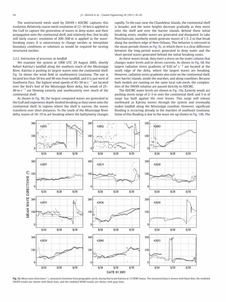
Fig. 14. Hurricane Katrina significant wave heights (m); mean wave directions (°), measuremeasured data is shownwith black dots, themodeled SWAN results are shownwith black linwas collected by WAVCIS (http://www.wavcis.lsu.edu).

bias in SWAN is caused mostly by a time shift between its results andthe measured data; SWAN does not match exactly the timing of thepeak. The SI errors are large compared to other wave studies (Cardoneet al., 1996; Janssen, 2004), but they reflect the complexities ofmodeling hurricane systems that change rapidly over multiple scales.In deep water, the errors in the SWAN results are only slightly largerthan in theWAM results, even though the SWANmesh spacing of 12–18 km is much larger than WAM's regular mesh spacing of 5 km.

It is more difficult to validate SWAN in shallow water because ofthe scarcity of nearshore measurement data. The Coastal StudiesInstitute at Louisiana State University operates two gauges south ofTerrebonne Bay, as shown in Fig. 7 (http://www.wavcis.lsu.edu).Stations CSI05 and CSI06 are located in water depths of about 7 m and20 m, respectively, so they experience the nearshore physics ofbottom friction, triad wave–wave interactions and depth-inducedbreaking. As shown in Fig. 14, SWAN matches well the waveparameters at these stations. As shown in Table 4, the average errorsproduced by WAM/STWAVE are somewhat smaller than thoseproduced by SWAN, presumably because of the better estimate ofthe deep-water wave conditions.

The ADCIRC water levels have been validated to high-water marks(HWMs) collected at 206 stations by the USACE and 193 stations byURS/FEMA (Ebersole et al., 2007; URS, 2006a). These HWMs includethe effects of surge and wave set-up but not wind waves. ADCIRCpredicts well the majority of the HWMs, with most locations havingdifferences less than 0.5 m. Comparisons of measured-to-modeledHWMs have best-fit slopes of 0.98–1.02 and correlation coefficients R2

of 0.92–0.94. Differences occur in places where the resolution isinsufficient, such as on the south shore of Lake Pontchartrain, but thematch to the HWMs is much better in regions near open water.Average magnitudes and standard deviations of the differences were

d clockwise from geographic north; and mean wave periods (s) at two CSI buoys. Thees, and themodeledWAM/STWAVE results are shownwith gray lines. The CSI buoy data

57J.C. Dietrich et al. / Coastal Engineering 58 (2011) 45–65

computed, bothwith andwithout the errors in themeasurement data,and those values are summarized in Table 5. When we account for theHWM uncertainties, the estimated average absolute model error is0.26–0.27 m, and the standard deviation is 0.41–0.44 m.

These error statistics are similar to results obtained from theloose coupling of ADCIRC to the structured wave models WAM andSTWAVE (Bunya et al., 2010). In addition, a qualitative comparison

Fig. 15. Hurricane Rita significant wave height contours (m) and wind speed vectors (m s−

times: (a) 1800 UTC 21 September 2005, (b) 0600 UTC 22 September 2005, (c) 1800 UTC2005 and (f) 0600 UTC 24 September 2005.

to that study shows the SWAN+ADCIRC solution is remarkablysimilar. Because the wave set-up in Fig. 10b is shown near the peakof the hurricane, it can be compared to the maximum wave set-upobtained from the loose coupling (Dietrich et al., 2010). Bothcoupled models create set-up of 0.8 m over the Mississippi Riverdelta and 0.2–0.3 m over much of the region. WAM/STWAVE isslightly more focused, with higher wave set-up behind the barrier

1) at 12-h intervals in the Gulf of Mexico. The six panels correspond to the following22 September 2005, (d) 0600 UTC 23 September 2005, (e) 1800 UTC 23 September

58 J.C. Dietrich et al. / Coastal Engineering 58 (2011) 45–65

islands, whereas SWAN wave breaking is spread farther onto thecontinental shelf.

3.3. Hurricane Rita

Like Katrina, Rita was a powerful and destructive hurricane duringthe 2005 season. However, it pushed farther to the west and madelandfall near the Louisiana–Texas border. In southwest Louisiana, abroad continental shelf distributed the wave breaking over a largerdistance, while the lack of protruding geographic features preventedthe early build-up of storm surge. These distinctions caused waves todevelop and propagate differently during Rita, thus making it a goodtest of SWAN+ADCIRC.

3.3.1. Evolution of waves in deep waterRita created large waves throughout the Gulf of Mexico. As shown

in Fig. 15a, 60 h before landfall, the storm was well into the Gulf andwas generating waves with significant heights very near theirmaximum of about 19 m. In addition, waves of 3–6 m propagatethroughout most of the Gulf. Rita moved northwestward through theregion, threatening Galveston and the Texas coastline before turningnorthward tomake landfall at Sabine Pass. On 23 September 2005, thestorm reached the continental shelf break, and its largest waves beganto spread and break. The symmetry of the wave field deteriorates asthe largest waves reach the shelf as shown in Fig. 15d and e. Finally, asRita moved over the shelf and made landfall, as shown in Fig. 15f, thelargest significant wave heights it generated were about 8 m. Thesewaves broke near the coastline and created set-up and currents insouthwest Louisiana.

Fig. 16. Hurricane Rita winds and waves at 0600 UTC 24 September 2005 in southeastern Laveraging period and at 10 m elevation; (b) significant wave height contours (m) and win(d) radiation stress gradient contours (m2 s−2) and wind vectors (m s−1).

3.3.2. Interaction of processes at landfallWe examine all aspects of the coupled system as they interact at

0600 UTC 24 September 2005, when Rita was located about 35 kmand 2 h from landfall. As shown in Fig. 16a, its eye was located on thecontinental shelf, and its maximum wind speeds reduced to 40–45 m s−1. Because of the storm's northwestward track, its winds blewparallel to the coastline in southwest Louisiana for hours beforelandfall. It is only at this relatively late stage in the hurricane that thewinds are changing to blow inland.

The shelf has a dramatic effect on the SWAN wave solution. InFig. 16b, the significant wave heights decreased from their maximumof about 19 m in the Gulf; now the maximum wave heights are about8 m. Note the depth-induced breaking as the waves approach thecoastline, and especially near the Tiger and Trinity Shoals (shown inFig. 7). The wave heights decrease to 2.5–3 m over the shoals and lessat the coastline. Waves of 1–1.5 m are generated inside Vermilion Bay,while waves of 1 m are generated inside Calcasieu and White Lakes.This behavior is also seen in Fig. 16c, in which sharp gradients in themean wave periods are observed in the wave-breaking zones, andsmaller periods are seen in the bays and lakes. A broad swath of meanperiods of 7–9 s exists on the continental shelf, but the periodsdecrease as the large waves break.

As shown in Fig. 16d, the radiation stress gradients are near theirmaximum in regions with significant wave breaking, such as along thecoastline and the shoals. The radiation stress gradients reach 0.005–0.02 m2 s−2 in these regions. However, significant gradients are alsolocated at the northeast shores of the inland water bodies andchannels, as waves break in these regions. The largest gradients occurto the east, nearer to Timbalier Bay, where the hurricane is pushing

ouisiana. The panels are: (a) wind contours and vectors (m s−1), shown with a 10 mind vectors (m s−1); (c) mean wave period contours (s) and wind vectors (m s−1); and

59J.C. Dietrich et al. / Coastal Engineering 58 (2011) 45–65

large waves onto the relatively narrow shelf, creating large radiationstress gradients and set-up.

As shown in Fig. 17a, the storm surge has not yet pushed coastalwater onshore, but the overland flooding due to the lakes and bays isevident. In the four lakes, strong east–west gradients are observed,with eastern drawdown and western flooding. Easterly winds havepushed water from these lakes and into the surrounding marshes.Storm surge builds at the coastline as the winds change to blowonshore; the maximum storm surge of 4.7 m occurs near CalcasieuPass as Rita makes landfall. As shown in Fig. 17b, at the coastline nearSabine and Calcasieu Lakes, the wave set-up is about 0.05–0.1 m,while it is 0.1–0.2 m near Vermilion Bay. The difference is caused bythe shoals, which reach farther onto the shelf, where the larger wavesare breaking. This set-up represents 2–5% of the overall water levelsnear the coastline, and 10–20% of the overall water levels fartherinland.

The winds and waves also drive currents, as shown in Fig. 17c. Inthe region nearest the eye of the hurricane and its maximum-strengthwinds, the currents range from 1 to 2 m s−1. The winds havedeveloped surge on the continental shelf, and now they are pushingit into southwest Louisiana. There are also several localized instancesof significant currents, such as the channel connecting Vermilion Bayto the Gulf, where the currents range from 1.5 to 2 m s−1 as waterflows into the bay. Currents are caused by gradients in the waterlevels, but they are also caused by the wave breaking, as shown inFig. 17d. The wave-driven currents are focused where the wavesbreak, including in the channel near Vermilion Bay, along the coastlineand near the shoals.

Fig. 17. Hurricane Rita water levels and currents at 0600 UTC 24 September 2005 in southeas(b) wave-driven set-up contours (m) and wind vectors (m s−1); (c) current contours (m s−

vectors (m s−1).

3.3.3. Validation of coupled modelThe SWAN wave solution for Rita has been compared to measured

results from NDBC buoys. The significant wave heights in Fig. 18match well in regions with sufficient resolution, including the buoyson the continental shelf on either side of the storm track. At somestations near the track, however, the match is not as good. At buoy42001, over which Rita passed while it was still a category-4 storm,the modeled peak height of 15 m is much larger than the measuredpeak height of 11 m. The mesh resolution of 12–18 km may be toolarge in this region. The mean directions (Fig. 19) and mean periods(Fig. 20) also show good agreement. At buoys to the east of the track,the waves change directions from northerly (0°) to southerly (180°)as the storm passes. This trend is reversed to the west of the track, asthe waves change directions from easterly (90°) to northerly (0°). Asthe storm passes these buoys, the periods roughly double, from 4–6 sto about 10–12 s, and then decrease slowly as long waves continue tobe generated by the storm. As shown in Table 3, the SWAN and WAMresults are comparable, with average SI errors for the significant waveheights of 0.35 and 0.32, respectively. On a mesh with much coarserresolution in deep water, SWAN is similar to WAM, while offeringincreased resolution near the coastline and the efficiencies associatedwith tight coupling.

In shallow water, SWAN has been validated to the CSI measureddata shown in Fig. 21. Note the gauge at station CSI06 failed duringKatrina and had not been repaired when Rita passed through theGulf. However, modeled SWAN results match well with themeasured data at CSI05. The significant wave heights reach theirmaximum of about 2.5 m as the storm moved toward landfall, and

tern Louisiana. The panels are: (a) water level contours (m) and wind vectors (m s−1);1) and wind vectors (m s−1); and (d) wave-driven current contours (m s−1) and wind

Fig. 18. Significant wave heights (m) during Hurricane Rita at 12 NDBC buoys. The measured data is shown with black dots, the modeled SWAN results are shown with black lines,and the modeled WAM results are shown with gray lines.

60 J.C. Dietrich et al. / Coastal Engineering 58 (2011) 45–65

the mean periods jumped from about 5 s to 7–8 s. As shown inTable 4, the average errors produced by WAM/STWAVE aresomewhat smaller than to those produced by SWAN, presumablybecause of the better estimate of the deep-water wave conditions(see previous discussion). A better representation of wave physicsin the deeper Gulf in SWAN might lead to better results at thesenearshore stations.

The ADCIRC solution has been validated to a set of 80 high-watermarks collected by URS/FEMA (URS, 2006b). ADCIRC matches wellthe HWMs, with most points falling within an error of 0.5 m. Acomparison of measured-to-modeled HWMs shows a best-fit slopeof 0.94 and a correlation coefficient R2 of 0.75. The significantdifferences occur near Vermilion Bay, where the modeled HWMs aremuch lower than those measured by URS/FEMA. This could be dueto a lack of mesh resolution in this region or the viscous muddybottom of Vermilion Bay (Sheremet et al., 2005; Stone et al., 2003).The removal of these points from the error statistics would increasethe best-fit slope to 1.01 and the correlation coefficient R2 to 0.85. Asnoted in Table 5, when the HWM uncertainties are disregarded, theestimated average absolute model error is 0.18–0.24 m, and thestandard deviation is 0.33–0.39 m. These results are similar to theloose coupling of ADCIRC with WAM and STWAVE (Bunya et al.,2010).

3.4. Computational performance

SWAN+ADCIRC was benchmarked on Ranger, which is a SunConstellation Linux Cluster at the Texas Advanced Computing Center(TACC) (http://www.tacc.utexas.edu). Ranger consists of 3936 SMPcompute nodes, each with four quad-core AMD Opteron processors.The nodes are connected with an InfiniBand network with abandwidth of 1 GB s−1. The overall system has 62,976 cores, 123 TBof memory and a theoretical peak performance of 579 TFLOPS.

The Katrina simulation described previously was run with thecoupled model and again with its individual components in order todiscern coupling effects on simulation times. When ADCIRC was runindividually, it did not receive radiation stress gradients from anysource. When SWAN was run individually, it read the wind speedsfrom external files, but it did not receive water levels or currents fromany source. The models were run on 256 to 5120 cores, of which tencores were always dedicated for file output by ADCIRC. Wall-clocktimes were reported by the Sun Grid Engine batch system.

As shown in Fig. 22, the individual SWAN and ADCIRCmodels bothscale linearly through about 1000–1500 cores, but they diverge athigher numbers of computational cores. ADCIRC's timing results leveloff, because the global communication associated with its implicit,conjugate-gradient solver begins to dominate the simulation time.

Fig. 19. Mean wave directions (°), measured clockwise from geographic north, during Hurricane Rita at 12 NDBC buoys. The measured data is shown with black dots, the modeledSWAN results are shown with black lines, and the modeled WAM results are shown with gray lines.

61J.C. Dietrich et al. / Coastal Engineering 58 (2011) 45–65

The highly localized solution procedure in SWAN allows it to scalelinearly through 5000 cores, enabling performance of less than 10 minper day of Katrina simulation.

In the SWAN+ADCIRC timing results, note the sharp increase inperformance between 246 and 374 computational cores, whichsuggests that the coupled model requires less than about 8000mesh vertices per core to maintain memory in cache. Also note thatthe coupled model shows linear scaling to about 3000 computationalcores, but then it levels off. At this point, the communication overheadfrom ADCIRC slows down the coupled model. However, theperformance in this range is about 24 min per day of Katrinasimulation, which is sufficient for forecasts of large storms.

With the exception of the run on 246 cores, when the combinedproblem size was too large to maintain in cache, the SWAN+ADCIRCtiming results are never larger than the combination of the timingresults from each component. The tight coupling adds no overhead tothe simulation, and it even increases the efficiency at large numbers ofcores. For example, at 3062 cores, the SWAN+ADCIRC timing of24 min per day is less than the combined total of 20 min per day forADCIRC and 11 min per day for SWAN. This efficiency is created by thesharing of tasks, such as the reading and interpolation of the windinput files. In addition, the computational load per file output intervalis increased in the coupled model, so the dedicated file output cores

havemore time to complete their tasks while the computational coresare working. Thus, at large numbers of cores, it is faster to run thecoupled model than its components individually.

4. Conclusions

The recent introduction of the unstructured-mesh SWAN allowsfor wave simulation on the same unstructured meshes used byADCIRC, which utilizes basin-to-floodplain scale domains andincreases locally the resolution in regions with large spatial gradients.This work implemented the tight coupling of SWAN+ADCIRC, so thatthese models run as an integrated system on the same mesh, andvertex-based solutions and forcing information are passed throughlocal memory or cache.

SWAN+ADCIRC simulates hurricane storm surge with high levelsof accuracy. Hindcasts of Katrina and Rita show that the modelsgenerate waves in deep water; dissipate waves due to changes inwave–wave interactions, bathymetry and bottom friction in southernLouisiana; apply the radiation stress gradients to create set-up andwave-driven currents in the circulation model; and then return thosewater levels and currents to the wave model. SWAN compares well tomeasured wave parameters at 12 NDBC buoys in the Gulf, eventhough the mesh resolution is 12–18 km in those areas. Major

Fig. 20.Mean wave periods (s) during Hurricane Rita at 12 NDBC buoys. The measured data is shown with black dots, the modeled SWAN results are shown with black lines, and themodeled WAM results are shown with gray lines.

62 J.C. Dietrich et al. / Coastal Engineering 58 (2011) 45–65

differences were at buoys located west of the hurricane track, whereSWAN+ADCIRC tends to over-predict the significant wave heights.This over-prediction may be due to missing physics (such as thewarm-core eddy) or poor numerics (such as the coarseness of themesh). In the nearshore, validation of SWAN to measured data at twoCSI stations showed that SWAN matches well the wave behavior onthe continental shelf. The ADCIRC modeled water levels compare wellwith measured HWMs. Comparisons to WAM and STWAVE showedthat the errors in the SWAN results are slightly larger than in theWAM/STWAVE results, which may be due to a larger mesh size forSWAN in deep water. SWAN's physics can be optimized for deep

Table 3Summary of average errors at the NDBC buoys for the SWAN andWAM simulations of KatrinBias error metrics were computed using Eqs. (12) and (13) (but they have not been normalreflect the differences in the time periods over which the errors were computed.

Storm Model Significant heights Mean dire

SI Relative Bias Mean Obs. (m) RMS (°)

Katrina SWAN 0.44 0.077 1.87 37.8WAM 0.36 −0.038 1.71 49.7

Rita SWAN 0.35 0.094 1.98 36.5WAM 0.32 −0.104 1.97 45.1

water, and it is well-positioned to increase its localized resolution toimprove accuracy in the future.

SWAN+ADCIRC is also highly efficient. It eliminates the need forinterpolation between models with heterogeneous meshes, interpo-lation at the boundaries of nested meshes, and the consideration ofoverlapping or inconsistent solutions. It shows linear scaling to about2000 cores and wall-clock times of 24 min per day of Katrinasimulation on a mesh with 2.4 million vertices. The coupled modelmaintains linear scaling to larger numbers of computational coreswhen applied to meshes with larger numbers of vertices. It does notadd overhead due to interpolation, global communication or the

a and Rita during the time periods shown in Table 2. The Scatter Index (SI) and Relativeized for the mean directions). The differences in the mean observations for each model

ctions Mean periods

Bias (°) Mean Obs. (°) SI Relative Bias Mean Obs. (s)

−9.0 136.7 0.22 −0.140 6.53−13.0 134.7 0.18 0.182 6.43

0.9 126.5 0.21 −0.156 6.740.2 127.0 0.16 0.012 6.73

Fig. 21. Hurricane Rita significant wave heights (m); mean wave directions (°), measured clockwise from geographic north; and mean wave periods (s) at two CSI buoys. Themeasured data is shown with black dots, the modeled SWAN results are shown with black lines, and the modeled STWAVE results are shown with gray lines. Note that buoy CSI 06did not record during the storm. The CSI buoy data was collected by WAVCIS (http://www.wavcis.lsu.edu).

Table 4Summary of errors for the SWAN andWAM/STWAVE simulations of Katrina and Rita during the time periods shown in Table 2. Note that buoy CSI06 did not record during Rita. TheScatter Index (SI) and Relative Bias error metrics were computed using Eqs. (12) and (13) (but they have not been normalized for mean directions). The differences in the meanobservations for each model reflect the differences in the time periods over which the errors were computed.

Storm Gauge Model Significant heights Mean directions Mean periods

SI Relative Bias Mean Obs. (m) RMS (°) Bias (°) Mean Obs. (°) SI Relative Bias Mean Obs. (s)

Katrina CSI05 SWAN 0.34 −0.029 0.73 52.7 21.0 123.9 0.29 −0.174 4.84WAM/STWAVE 0.20 0.073 1.70 75.6 61.5 120.8 0.70 0.510 5.67

CSI06 SWAN 0.16 −0.001 0.90 64.1 −34.4 132.9 0.32 −0.249 5.14WAM/STWAVE 0.06 0.030 3.87 25.2 −23.3 143.8 0.29 0.291 8.25

Rita CSI05 SWAN 0.18 −0.127 1.13 40.2 22.8 123.5 0.25 −0.084 5.03WAM/STWAVE 0.10 −0.002 2.50 44.4 43.9 124.5 0.78 0.741 5.90

CSI06 SWAN – – – – – –

WAM/STWAVE – – – – – –

63J.C. Dietrich et al. / Coastal Engineering 58 (2011) 45–65

mechanics of managing the coupling. Instead, SWAN+ADCIRC sharesthe work among model components in a way that can speed up thecombined run time. The result is a coupled model that is well-positioned for applications in high-performance computingenvironments.

Table 5Summary of difference/error statistics for the Katrina and Rita HWM data sets. Average abs

Storm Dataset

ADCIRC to measured HWMs Measured H

Average absolute difference Standard deviation Average abso

Katrina USACE 0.40 0.47 0.13Katrina URS 0.36 0.44 0.10Rita URS 0.34 0.43 0.10Rita (no VB) URS 0.28 0.38 0.11

Future work will improve the efficiency and accuracy of thecoupled model. The new generation of computational meshes insouthern Louisiana and Texas will increase resolution in the wave-generation zones in the Gulf of Mexico, the wave-breaking zonesalong the coastline and the barrier islands, and the channels and inlets

olute differences/errors and standard deviations are given in m.

WMs Estimated ADCIRC errors

lute difference Standard deviation Average absolute error Standard deviation

0.18 0.27 0.440.16 0.26 0.410.18 0.24 0.390.19 0.18 0.33

Fig. 22. Timing results for SWAN+ADCIRC and its components on the TACC Ranger machine. The times shown are wall-clock minutes per day of Katrina simulation on the SL15mesh. SWAN results are shown in red, ADCIRC results are shown in blue, and SWAN+ADCIRC results are shown in purple.

64 J.C. Dietrich et al. / Coastal Engineering 58 (2011) 45–65

further inland. Future generations of meshes will relax initially theresolution and then refine adaptively, by adding resolution in regionswhere the computed gradients are large in either model component.Thesemesheswill represent better thewave and circulation solutions,and the highly-efficient, coupled model will allow them to be usedoperationally. The tight coupling of SWAN+ADCIRC enables waves,water levels and currents to interact in complex problems and in away that is accurate and efficient.

Acknowledgements

This work was supported by awards from the Office of NavalResearch (N00014-06-1-0285), the National Science Foundation(DMS-0620697, DMS-0620696, DMS-0620791, OCI-0749015 andOCI-0746232), and the US Department of Homeland Security (2008-ST-061-ND-0001). Computational resources were provided in part byan award from the TACC and the TeraGrid project (TG-DMS080016N).The views and conclusions contained in this document are those ofthe authors and should not be interpreted as necessarily representingthe official policies, either expressed or implied, of the US Departmentof Homeland Security. Permission to publish this work was obtainedfrom the US Army Corps of Engineers.

References

Atkinson, J.H., Westerink, J.J., Hervouet, J.M., 2004. Similarities between the waveequation and the quasi-bubble solutions to the shallow water equations.International Journal for Numerical Methods in Fluids 45, 689–714.

Battjes, J.A., 1972. Radiation stresses in short-crested waves. Journal of Marine Research30 (1), 56–64.

Battjes, J.A., Janssen, J.P.F.M., 1978. Energy loss and set-up due to breaking of randomwaves. Proceedings of the 16th International Conference on Coastal Engineering,ASCE, pp. 569–587.

Booij, N., Ris, R.C., Holthuijsen, L.H., 1999. A third-generation wave model for coastalregions, Part I, model description and validation. Journal of Geophysical Research104, 7649–7666.

Bunya, S., Dietrich, J.C., Westerink, J.J., Ebersole, B.A., Smith, J.M., Atkinson, J.H., et al.,2010. A high resolution coupled riverine flow, tide, wind, wind wave and stormsurge model for southern Louisiana and Mississippi: Part I — model developmentand validation. Monthly Weather Review 138, 345–377.

Cardone, V.J., Jensen, R.E., Resio, D.T., Swail, V.R., Cox, A.T., 1996. Evaluation ofcontemporary ocean wave models in rare extreme events: the “Halloween Storm”of October 1991 and the “Storm of the Century” of March 1993. Journal ofAtmospheric and Oceanic Technology 13 (1), 198–230.

Cardone, V.J., Cox, A.T., Forristall, G.Z., 2007. OTC 18652: hindcast of winds, waves andcurrents in Northern Gulf of Mexico in Hurricanes Katrina (2005) and Rita (2005).2007 Offshore Technology Conference, Houston, TX.

Chen, Q., Wang, L., Tawes, R., 2008. Hydrodynamic response of Northeastern Gulf ofMexico to hurricanes. Estuaries and Coasts 31 (6), 1098–1116.

Collins, N., Theurich, G., DeLuca, C., Suarez, M., Trayanov, A., Balaji, V., et al., 2005. Designand implementation of components in the earth system modeling framework.International Journal of High Performance Computing Applications 19 (3), 341–350.

Cox, A.T., Greenwood, J.A., Cardone, V.J., Swail, V.R., 1995. An interactive objectivekinematic analysis system. Fourth International Workshop onWave Hindcasting andForecasting, Banff, Alberta. Atmospheric Environment Service, Canada, pp. 109–118.

Dawson, C., Westerink, J.J., Feyen, J.C., Pothina, D., 2006. Continuous, discontinuous andcoupled discontinuous–continuous galerkin finite element methods for the shallowwater equations. International Journal for Numerical Methods in Fluids 52, 63–88.

Dietrich, J.C., Bunya, S.,Westerink, J.J., Ebersole, B.A., Smith, J.M., Atkinson, J.H., et al., 2010.Ahigh resolution coupled riverine flow, tide, wind, wind wave and storm surge modelfor southern Louisiana and Mississippi: Part II— synoptic description and analyses ofHurricanes Katrina and Rita. Monthly Weather Review 138, 378–404.

Ebersole, B.A., Westerink, J.J., Resio, D.T., Dean, R.G., 2007. Performance evaluation of theNew Orleans and Southeast Louisiana Hurricane Protection System, Volume IV— thestorm. Final Report of the Interagency Performance Evaluation Task Force. U.S. ArmyCorps of Engineers, Washington, D.C.

Eldeberky Y. Nonlinear transformation of wave spectra in the nearshore zone. Ph.D.thesis, Delft University of Technology, Delft, The Netherlands 1996.

Funakoshi, Y., Hagen, S.C., Bacopoulos, P., 2008. Coupling of hydrodynamic and wavemodels: case study for Hurricane Floyd (1999) hindcast. ASCE Journal ofWaterway,Port, Coastal and Ocean Engineering 134 (6), 321–335.

Garratt, J.R., 1977. Review of drag coefficients over oceans and continents. MonthlyWeather Review 105, 915–929.

Gorman, R.M., Neilson, C.G., 1999. Modelling shallow water wave generation andtransformation in an intertidal estuary. Coastal Engineering 36, 197–217.

Gregersen, J.B., Gijsbers, P.J.A., Westen, S.J.P., Blind, M., 2005. OpenMI: the essentialconcepts and their implications for legacy software. Advances inGeosciences 4, 37–44.

Gunther, H., 2005. WAM Cycle 4.5 Version 2.0, Institute for Coastal Research. GKSSResearch Centre Geesthacht.

Hasselmann, K., 1974. On the spectral dissipation of ocean waves due to whitecapping.Boundary-Layer Meteorology 6, 107–127.

Hasselmann, K., Barnett, T.P., Bouws, E., Carlson, H., Cartwright, D.E., Enke, K., et al.,1973. Measurements of wind–wave growth and swell decay during the Joint NorthSea Wave Project (JONSWAP). Ergnzungsheft zur Deutschen HydrographischenZeitschrift Reihe 12 (A8).

Hasselmann, S., Hasselmann, K., Allender, J.H., Barnett, T.P., 1985. Computations andparameterizations of the nonlinear energy transfer in a gravity wave spectrum. PartII: parameterizations of the nonlinear transfer for application in wave models.Journal of Physical Oceanography 15 (11), 1378–1391.

Hill, C., DeLuca, C., Balaji, V., Suarez, M., da Silva, A., 2004. Architecture of the EarthSystem Modeling Framework. Computing in Science and Engineering 6 (1).

Holthuijsen, L.H., Herman, A., Booij, N., 2003. Phase-decoupled refraction–diffractionfor spectral wave models. Coastal Engineering 49, 291–305.

Janssen, P., 2004. The Interaction of Ocean Waves and Wind. Cambridge UniversityPress, Cambridge.

Karypis, G., Kumar, V., 1999. A fast and high quality multilevel scheme for partitioningirregular graphs. SIAM Journal of Scientific Computing 20 (1), 359–392.

65J.C. Dietrich et al. / Coastal Engineering 58 (2011) 45–65

Kim, S.Y., Yasuda, T., Mase, H., 2008. Numerical analysis of effects of tidal variations onstorm surges and waves. Applied Ocean Research 30, 311–322.

Kolar, R.L., Westerink, J.J., Cantekin, M.E., Blain, C.A., 1994. Aspects of nonlinearsimulations using shallow water models based on the wave continuity equations.Computers and Fluids 23 (3), 1–24.

Komen, G., Cavaleri, L., Donelan, M., Hasselmann, K., Hasselmann, S., Janssen, P.A.E.M.,1994. Dynamics and Modeling of Ocean Waves. Cambridge University Press,Cambridge.

Longuet-Higgins, M.S., Stewart, R.W., 1964. Radiation stresses in water waves; physicaldiscussions, with applications. Deep Sea Research 11, 529–562.

Luettich, R.A., Westerink, J.J., 2004. Formulation and numerical implementation of the2D/3D ADCIRC Finite Element Model Version 44.XX. http://adcirc.org/adcirc_the-ory_2004_12_08.pdf2004.

Moore, R.V., Tindall, I., 2005. An overview of the open modelling interface andenvironment (the OpenMI). Environmental Science and Policy 8, 279–286.

Pandoe, W.W., Edge, B.L., 2008. Case study for a cohesive sediment transport model forMatagorda Bay, Texas, with coupled ADCIRC 2D-Transport and SWAN WaveModels. ASCE Journal of Hydraulic Engineering 134 (3), 303–314.

Powell, M., Houston, S., Reinhold, T., 1996. Hurricane Andrew's landfall in South Florida.Part I: standardizing measurements for documentation of surface windfields.Weather Forecasting 11, 304–328.

Powell, M., Houston, S., Amat, L., Morrisseau-Leroy, N., 1998. The HRD real-timehurricane wind analysis system. Journal of Wind Engineering and IndustrialAerodynamics 77–78, 53–64.

Ris, R.C., Booij, N., Holthuijsen, L.H., 1999. A third-generation wave model for coastalregions, Part II, verification. Journal of Geophysical Research 104, 7667–7681.

Rogers, W.E., Hwang, P.A., Wang, D.W., 2003. Investigation of wave growth and decay inthe SWAN model: three regional-scale applications. Journal of Physical Oceanog-raphy 33, 366–389.

Sheremet, A., Mehta, A.J., Liu, B., Stone, G.W., 2005. Wave–sediment interaction on amuddy inner shelf during Hurricane Claudette. Estuarine, Coastal and Shelf Science63, 225–233.

Smith, J.M., Sherlock, A.R., Resio, D.T., 2001. STWAVE: Steady-State Spectral Wave ModelUser's Manual for STWAVE, Version 3.0. USACE, Engineer Research and DevelopmentCenter. Technical Report ERDC/CHL SR-01-1, Vicksburg, MS. http://chl.erdc.usace.army.mil/Media/2/4/4/erdc-chl-sr-01-11.pdf.

Snyder, R.L., Dobson, F.W., Elliott, J.A., Long, R.B., 1981. Array measurements of atmosphericpressurefluctuationsabovesurfacegravitywaves. Journal of FluidMechanics 102, 1–59.

Stone, G.W., Sheremet, A., Zhang, X., He, Q., Liu, B., Strong, B., 2003. Landfall of twotropical systems seven days apart along southcentral Louisiana, USA. Proceedings ofCoastal Sediments '03, Clearwater Beach, Florida, USA, pp. 333–334.

Thompson, E.F., Smith, J.M., Miller, H.C., 2004. Wave transformation modeling at CapeFear River Entrance, North Carolina. J. Coastal Research 20 (4), 1135–1154.

Tolman, H.L., 2009. Usermanual and system documentation ofWAVEWATCH III version3.14. NOAA / NWS / NCEP / MMAB Technical Note 276.

URS, 2006a. Final coastal and riverine high-water marks collection for HurricaneKatrina in Louisiana. Final Report for the Federal Emergency Management Agency.

URS, 2006b. Final coastal and riverine high-water marks collection for Hurricane Rita inTexas. Final Report for the Federal Emergency Management Agency.

WAMDI Group, 1988. The WAM model — a third generation ocean wave predictionmodel. J. Phys. Oceanogr. 18, 1775–1810.

Wang, D.P., Oey, L.Y., 2008. Hindcast of waves and currents in Hurricane Katrina.Bulletin of the American Meteorological Society 89 (4), 487–495.

Warner, J.C., Perlin, N., Skyllingstad, E.D., 2008. Using the model coupling toolkit tocouple earth system models. Environmental Modelling & Software 23, 1240–1249.

Weaver, R.J., Slinn, D.N., 2004. Effect of wave forcing on storm surge. Proceedings ofCoastal Engineering '04, Lisbon, Portugal, pp. 1532–1538.

Westerink, J.J., Luettich, R.A., Feyen, J.C., Atkinson, J.H., Dawson, C., Roberts, H.J., et al.,2008. A basin to channel scale unstructured grid hurricane storm surge modelapplied to southern Louisiana. Monthly Weather Review 136 (3), 833–864.

Wu, J., 1982. Wind-stress coefficients over sea surface from breeze to hurricane. Journalof Geophysical Research 87, 9704–9706.

Zijlema, M., 2010. Computation of wind–wave spectra in coastal waters with SWAN onunstructured grids. Coastal Engineering 57, 267–277.