
Modeling Fluid Systemsnhuttho/me584/Chapter 5 Fluid Systems_part 1.pdf–Common modeling principle...
28
Modeling Fluid Systems Dr. Nhut Ho ME584 Chp5 1
Transcript of Modeling Fluid Systemsnhuttho/me584/Chapter 5 Fluid Systems_part 1.pdf–Common modeling principle...

Modeling Fluid Systems
Dr. Nhut Ho
ME584
Chp5 1

Agenda
• Introduction
• Properties of Fluid and Reynolds Number Effects
• Passive Components
• Case Study: Spring-Loaded Diaphragm Actuator
• Active Learning: Pair-share Exercises, Case Study
Chp5 2

Introduction
• Fluid Systems– Operate through effects of either liquids or gases
– Have wide range of applications, e.g., vehicle suspension systems, hydraulic servomotors, and chemical processing systems
• Hydraulics (fluid is incompressible) and pneumatic (fluid is compressible) systems– Common modeling principle is conservation of mass
– Key advantages relative to electro-mechanical systems
• Power density of pump/actuators (1 order of mag. higher 200 psi electromagnetic actuator vs. 3000-8000 psi hydraulic actuators)
• Circulating fluid removes heat generated by actuator (instead of free or forced convection)
– Have more nonlinearities -> challenging for modeling and simulation
Chp5 3

Properties of Fluid
Chp5 4

Fluid Density
• Incompressible: density of fluid (e.g., liquid) remains constant despite changes in fluid pressure (an approximation, but simpler modeling)
• Compressible: density of fluid (e.g., gas) changes with pressure
• Liquids have higher density, absolute viscosity, bulk modulus, and exhibits surface tension effects
• Density of a fluid: mass m per unit volum V under pressure P0
and temperature T0
Chp5 5
Equation of State: Liquids
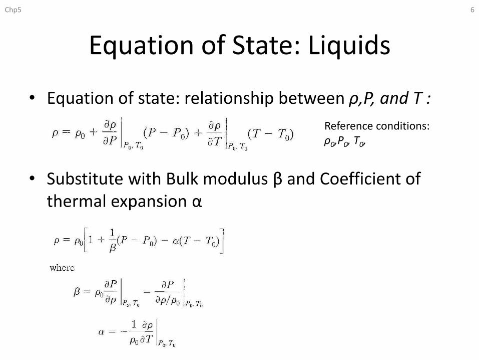
• Equation of state: relationship between ρ,P, and T :
• Substitute with Bulk modulus β and Coefficient of thermal expansion α
Chp5 6
Reference conditions: ρ0,P0, T0,
Equation of State: Liquids
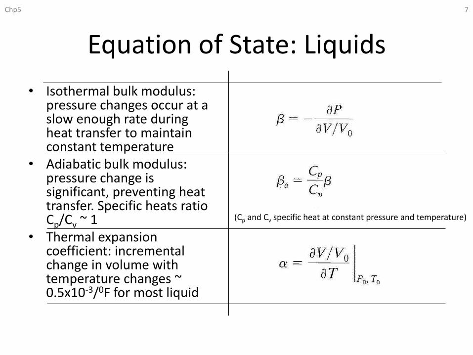
• Isothermal bulk modulus: pressure changes occur at a slow enough rate during heat transfer to maintain constant temperature
• Adiabatic bulk modulus: pressure change is significant, preventing heat transfer. Specific heats ratio Cp/Cv ~ 1
• Thermal expansion coefficient: incremental change in volume with temperature changes ~ 0.5x10⁻³/0F for most liquid
Chp5 7
(Cp and Cv specific heat at constant pressure and temperature)

Equation of State: Gases
• Ideal gas:
• Gas undergoing polytropic process:
• Bulk modulus:
Chp5 8
(βliquid ~ 5 to 15 Kbar >> β gas ~ 1 to 10 Bar)
Viscosity
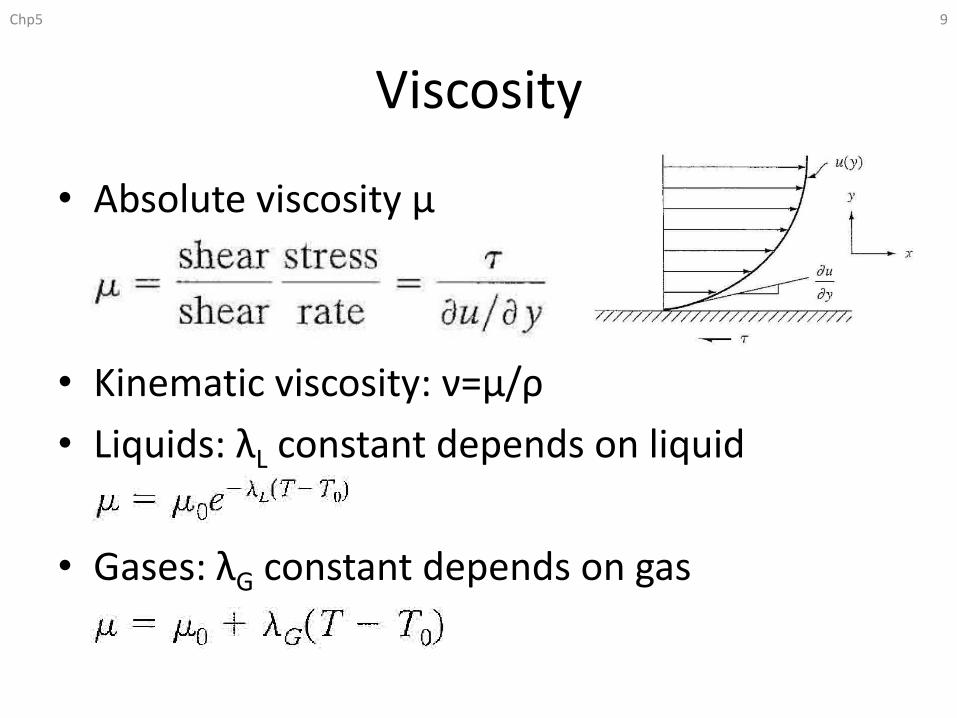
• Absolute viscosity μ
• Kinematic viscosity: ν=μ/ρ
• Liquids: λL constant depends on liquid
• Gases: λG constant depends on gas
Chp5 9
Speed of Sound, Specific Heat Ratio, and Reynolds Number
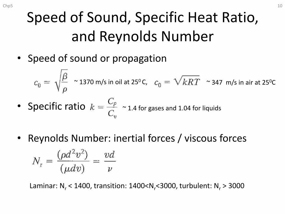
• Speed of sound or propagation
• Specific ratio
• Reynolds Number: inertial forces / viscous forces
Laminar: Nr < 1400, transition: 1400<Nr<3000, turbulent: Nr > 3000
Chp5 10
~ 1370 m/s in oil at 250 C, ~ 347 m/s in air at 250C
~ 1.4 for gases and 1.04 for liquids
Passive Components: Capacitance, Inductance, Resistance
Chp5 11

Chap5 12
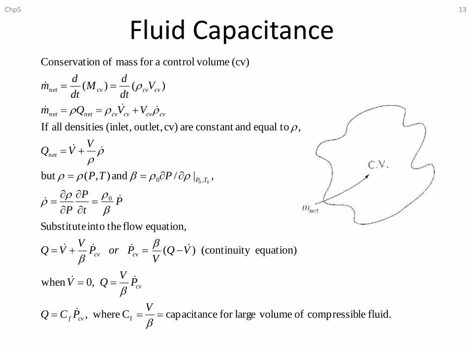
Fluid CapacitanceChp5 13
fluid. lecompressib of volumelargefor ecapacitanc C where,
,0when
equation)y (continuit)(
equation, flow theinto Substitute
,|/ and),(but
, toequal andconstant are cv) outlet, (inlet, densities all If
)()(
(cv) volumecontrol afor mass ofon Conservati
f
0
,0 00
VPCQ
PV
QV
VQV
PorPV
VQ
Pt
P
P
PTP
VVQ
VVQm
Vdt
dM
dt
dm
cvf
cv
cvcv
TP
net
cvcvcvcvnetnet
cvcvcvnet
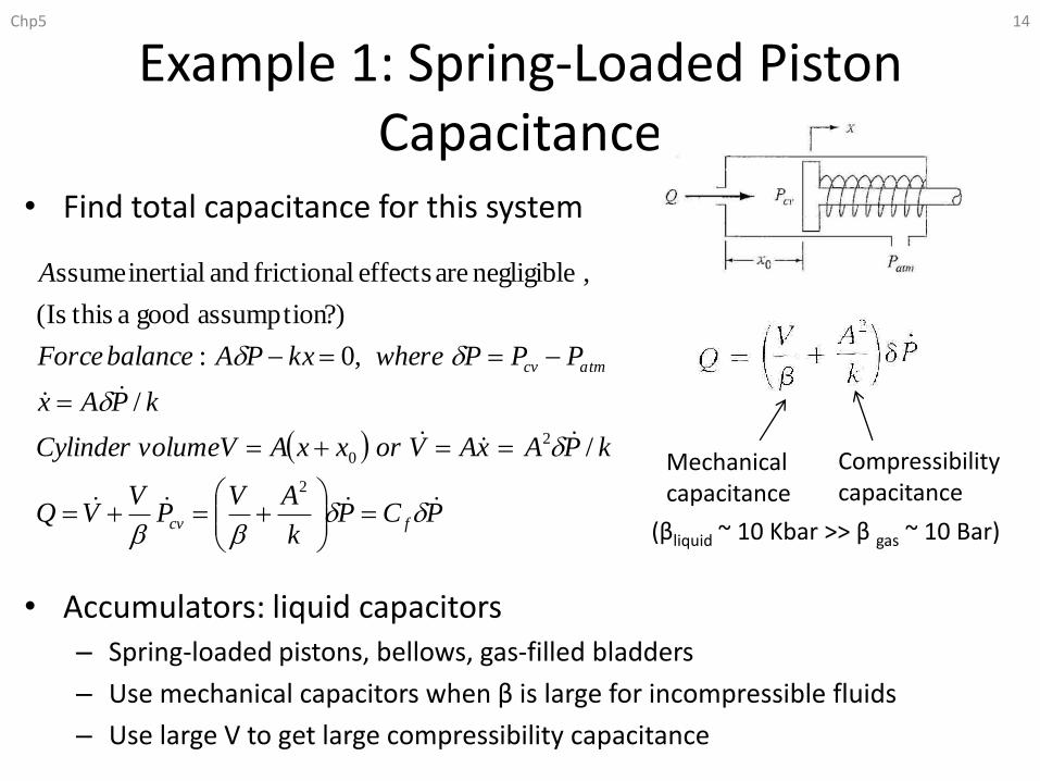
Example 1: Spring-Loaded Piston Capacitance
• Find total capacitance for this system
• Accumulators: liquid capacitors– Spring-loaded pistons, bellows, gas-filled bladders
– Use mechanical capacitors when β is large for incompressible fluids
– Use large V to get large compressibility capacitance
Chp5 14
Mechanical capacitance
Compressibility capacitance
(βliquid ~ 10 Kbar >> β gas ~ 10 Bar)
PCPk
AVP
VVQ
kPAxAVorxxAVvolumeCylinder
kPAx
PPPwherekxPAbalanceForce
A
fcv
atmcv
2
2
0 /
/
,0:
?)assumption good a thisIs(
,negligibleareeffectsfrictionalandinertialssume
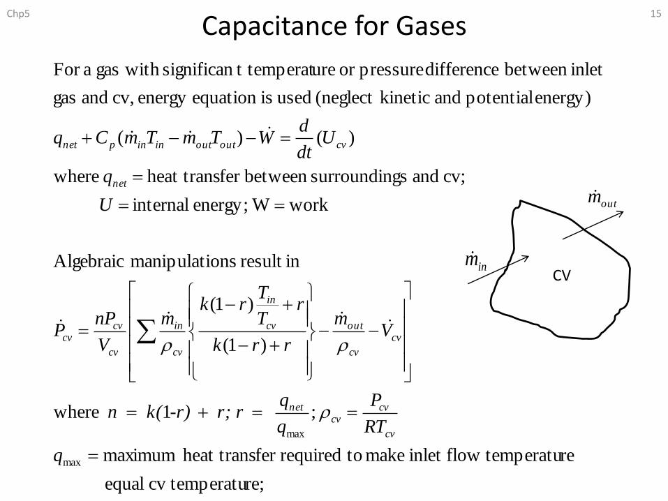
re; temperatucv equal
re temperatuflowinlet make torequiredfer heat trans maximum
;1 where
)1(
)1(
inresult onsmanipulati Algebraic
work Wenergy; internal
cv; and gssurroundinbetween fer heat trans where
)()(
energy) potential and kinetic(neglect used isequation energy cv, and gas
inlet between difference pressureor uret temperatsignifican with gas aFor
max
max
q
RT
P
q
q r; r -r) k(n
Vm
rrk
rT
Trk
m
V
nPP
U
q
Udt
dWTmTmCq
cv
cvcv
net
cv
cv
outcv
in
cv
in
cv
cvcv
net
cvoutoutininpnet
Capacitance for GasesChp5 15
CV
outm
inm
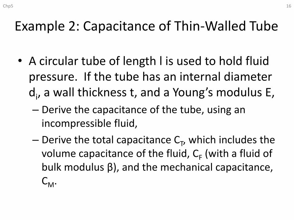
Example 2: Capacitance of Thin-Walled Tube
• A circular tube of length l is used to hold fluid pressure. If the tube has an internal diameter di, a wall thickness t, and a Young’s modulus E,
– Derive the capacitance of the tube, using an incompressible fluid,
– Derive the total capacitance CT, which includes the volume capacitance of the fluid, CF (with a fluid of bulk modulus β), and the mechanical capacitance, CM.
Chp5 16

Example 2: Capacitance of Thin-Walled Tube Chp5 17

Example 2: Capacitance of Thin-Walled Tube Chp5 18

Example 3: Pair-Share: Capacitance of a Balloon
The radius expansion, R-R0, of a balloon filled with a gas is directly proportional to the internal pressure of the gas. Let us write this proportionality as δP=K(R-R0). Derive an expression for the total capacitance of the balloon that considers the change in volume of the balloon and the effect of compressibility of the gas. (Volume = 4πR3/3)
Chp5 19

Example 3: Pair-Share: Capacitance of a Balloon
Chp5 20
CV
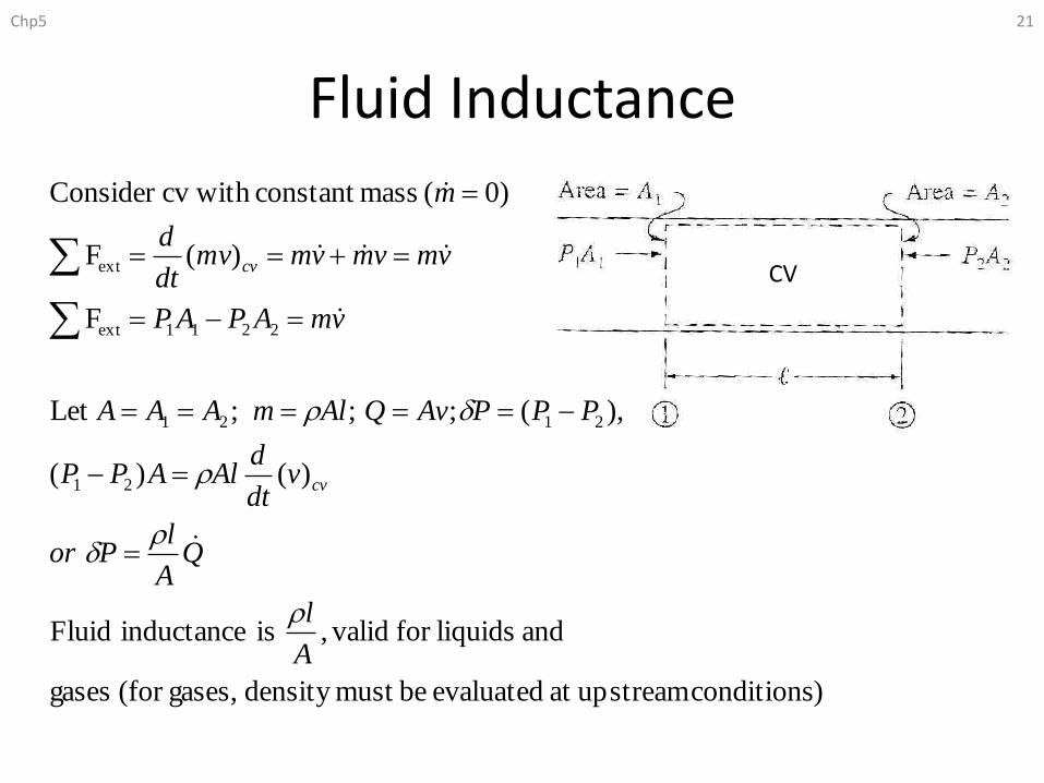
Fluid Inductance
Chp5 21
)conditions upstreamat evaluated bemust density gases,(for gases
and liquidsfor valid,isinductanceFluid
)()(
),(;;;Let
F
)(F
)0( massconstant with cvConsider
21
2121
2211ext
ext
A
l
QA
lPor
vdt
dAlAPP
PPPAvQAlmAAA
vmAPAP
vmvmvmmvdt
d
m
cv
cv

Fluid Resistance
• Laminar flow: viscous-dominated flow– Low enough flow rates or pressure drop in long capillary
tubes -> viscous flow
– Viscous terms dominate -> Reynolds is low (Nr < 1000)
• Orifice-type or head loss resistance: inertia-dominated flow– Orifice with short length in direction of flow
– Head loss with turbulent flow
• Compressible flow resistance– Similar to orifice type, but includes density variation of gas
– Flow equations have high degree of nonlinearity
Chp5 22
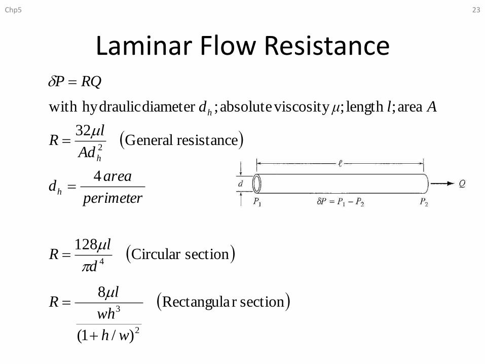
Laminar Flow Resistance
Chp5 23
A
sectionr Rectangula
)/1(
8
sectionCircular 128
4
resistance General32
area;length;viscosityabsolute;diameterhydraulicwith
2
3
4
2
wh
wh
lR
d
lR
perimeter
aread
Ad
lR
Alμd
RQP
h
h
h
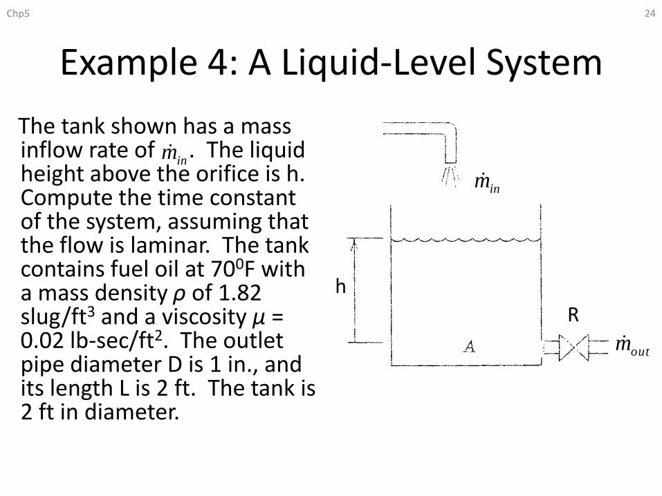
Example 4: A Liquid-Level System
The tank shown has a mass inflow rate of . The liquid height above the orifice is h. Compute the time constant of the system, assuming that the flow is laminar. The tank contains fuel oil at 700F with a mass density ρ of 1.82 slug/ft3 and a viscosity μ = 0.02 lb-sec/ft2. The outlet pipe diameter D is 1 in., and its length L is 2 ft. The tank is 2 ft in diameter.
Chp5 24
inm
R
h
inm
outm
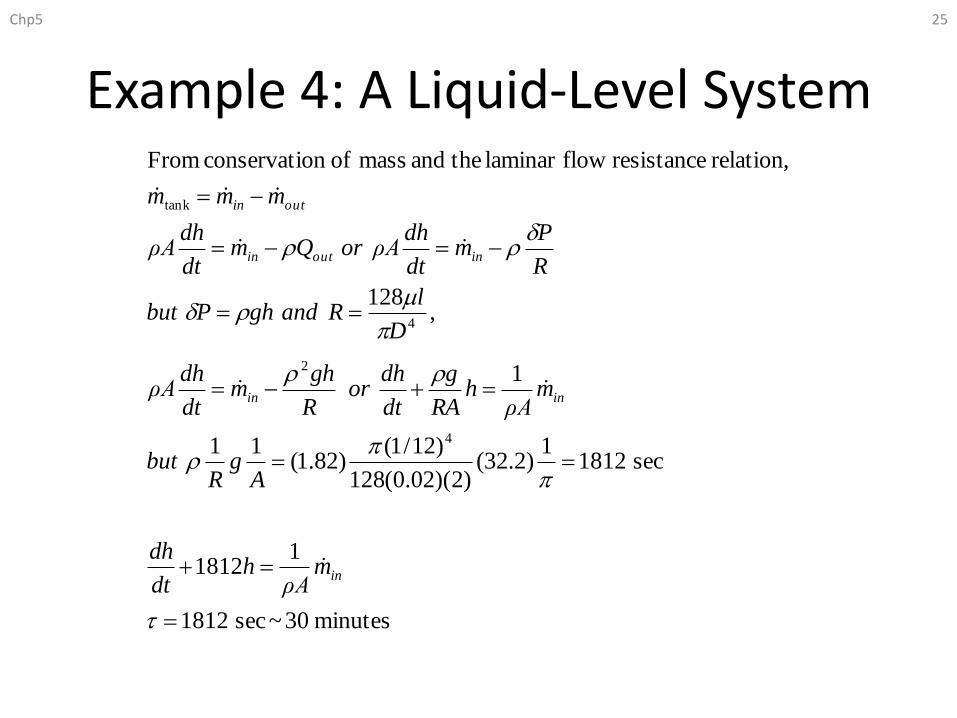
Example 4: A Liquid-Level System
Chp5 25
minutes30~sec1812
11812
sec18121
)2.32()2)(02.0(128
)12/1()82.1(
11
1
,128
relation, resistance flowlaminar theand mass ofon conservati From
4
2
4
tank
in
inin
inoutin
outin
mρA
hdt
dh
Ag
Rbut
mρA
hRA
g
dt
dhor
R
ghm
dt
dhρA
D
lRandghPbut
R
Pm
dt
dhρAorQm
dt
dhρA
mmm
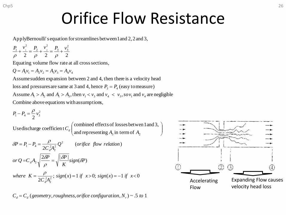
Orifice Flow ResistanceChp5 26
Accelerating Flow
Expanding Flow causes velocity head loss
15.~),,,(
01)(;01)(;2
)(||2
)(2
ofin termngrepresentiand
3,and1betwen lossesofeffectscombinedtcoefficiendischargeUse
2
s,assumptionwithequationsaboveCombine
negligibleare and, and then , and Assume
)measuretoeasy( hence 4, and 3at same are pressures and loss
head velocity a is e then ther,4 and 2between expansion sudden Assume
sections, cross allat rate flow volumeEquating
222
3,and22,and1betweensstreamlineforequationsBernoulli'Apply
2
2
2
2
2
2
2
241
23
2
341
4134313121
43
44332211
2
33
2
2
2
1 21
toNionconfiguratorificeroughnessgeometryCC
xifxsignxifxsignAC
Kwhere
PsignK
PPACQor
relationfloworificeQAC
PPP
AAC
vPP
vvso v vvvAAAA
PP
vAvAvAvAQ
vPvPvP
rdd
d
d
d
d

Example 5: Tank with an Orifice
• The tank shown has an orifice in its side wall. The orifice area is A0 and the bottom area of the tank is A. The liquid height above the orifice is h. The volume inflow rate is Qv. Develop a model of the height h with Qv as the input.
Chp5 27
Qv
AA0
h

Example 5: Tank with an Orifice
Chp5 28
ghACQdt
dhρA
ghPbut
PACQ
dt
dhρA
mmm
dv
dv
outin
2
,
2
relation, flow orifice theand mass ofon conservati From
0
0
tank
This is a nonlinear equation, how can it be analyzed?


![Procedural Fluid Modeling of Explosion Phenomena … · Procedural Fluid Modeling of Explosion Phenomena ... I.3.7 [Computer Graphics]: ... G. Kawada & T. Kanai / Procedural Fluid](https://static.fdocuments.us/doc/165x107/5b3fdc017f8b9aff118c9e34/procedural-fluid-modeling-of-explosion-phenomena-procedural-fluid-modeling-of.jpg)


