Modeling Dynamic Responses of Aircraft Environmental 1

Control Systems by Coupling with Cabin Thermal 2

Environment Simulations 3

4 Haishen Yin1, Xiong Shen1, Yan Huang1, Ran Duan1, Chao-Hsin Lin 2, Daniel Wei3, 5 Balasubramanyam Sasanapuri4 and Qingyan Chen1,5 6 1Tianjin Key Laboratory of Indoor Air Environmental Quality Control, School of Environmental Science 7 and Engineering, Tianjin University, Tianjin 300072, China 8 2Environmental Control Systems, Boeing Commercial Airplanes, Everett, WA 98203, USA 9 3Boeing Research & Technology - China, Beijing 100027, China 10 4ANSYS India Pvt Ltd, Pune, India 11 5School of Mechanical Engineering, Purdue University, West Lafayette, IN 47907, USA 12

Abstract 13

Commercial aircraft use environmental control systems (ECSs) to control the thermal 14 environment in cabins and thus ensure passengers’ safety, health, and comfort. This study 15 investigated the interaction between ECS operation and cabin thermal environment. 16 Simplified models were developed for the thermodynamic processes of the key ECS 17 components in a commercial software program, ANSYS Simplorer. A computational 18 fluid dynamics (CFD) program, ANSYS Fluent, was employed to simulate the thermal 19 environment in a cabin. Through the coupling of Simplorer and Fluent, a PID control 20 method was applied to the aircraft ECS in Simplorer to achieve dynamic control of the 21 temperature of the supply air to the cabin, which was used as a Fluent input. The 22 calculated supply air temperature agreed with the corresponding experimental data 23 obtained from an MD-82 aircraft on the ground. The coupled model was then used to 24 simulate a complete flight for the purpose of studying the interaction between ECS 25 operation and the cabin thermal environment. The results show that the PID controller in 26 the ECS can maintain the cabin air temperature within ±0.6 K of the set point, with an 27 acceptable air temperature distribution. The coupled models can be used for the design 28 and analysis of the ECS and cabin thermal environment for commercial airplanes. 29

30 Keywords: Thermal control, Temperature field, Aircraft ECS, Coupled Simulation 31

32

1 Introduction 33

Between 2005 and 2014, there were 12.6 billion air travellers worldwide, and the number 34 is increasing (World Bank Group 2015). In order to ensure passengers’ safety, health, and 35 comfort, the thermal environment in aircraft cabins should be controlled. On the ground, 36 an aircraft cabin can be very cold on a winter morning or very hot on a summer 37 afternoon. It is essential that the environmental control systems (ECSs) in aircraft be 38

Yin, H., Shen, X., Huang, Y., Feng, Z.，Long，Z., Duan, R., Lin, C.-H., Wei, D., Sasanapuri, B., and Chen, Q. 2016. “Modeling dynamic responses of aircraft environmental control systems by coupling with cabin thermal environment simulations,” Building Simulation, 9(4): 459-468.

2

capable of quickly heating up or cooling down cabins in order to provide an acceptable 39 thermal environment for passengers and crew members. Furthermore, during takeoff or 40 landing the aircraft is exposed to very rapid changes in outside air temperature and 41 pressure. For example, the outside air temperature at cruising altitude can be as low as -42 65 oC and the atmospheric pressure as low as 0.2 atm, while the corresponding 43 temperature and pressure at the sea level can be close to 0 oC and 1 atm. The ground air 44 temperature can be higher or lower than 0 oC in a typical winter day depending on the 45 location so does the outside air temperature at the cruising height. The ECS should be 46 able to rapidly respond to the outside environment and maintain a suitable temperature of 47 around 20 oC and a pressure equivalent to 2440 m above sea level (0.74 atm) inside the 48 air cabin (ASHRAE 2013). 49

In recent decades, there have been many investigations on ECSs and cabin 50 environments in aircraft. Eichler (1975) established several simplified models to 51 represent the dynamics of thermal controllers, valves, sensors, heat exchangers and 52 turbines of the ECS. Leo and Pérez-Grande (2005) employed other simplified models to 53 represent different ECS components in order to analyze the total performances. Zhao et 54 al. (2009) applied an experimental method to study ECS design and recommended that 55 off-design performance and dynamic response be taken into account in the design 56 process. Although these studies provided meaningful results, they addressed ECS 57 performance rather than the influence of cabin thermal environment on ECS response. 58 However, the cabin thermal environment is important for the thermal comfort and well-59 being of passengers and crew. Aircraft manufacturers have tried to make a better cabin 60 thermal environment. 61

Meanwhile, other studies have focused only on the cabin thermal environment. Some 62 of them have used experimental measurements in actual airplane cabins (Liu et al. 2012a; 63 Huang et al. 2015), mock-ups (Zhang et al. 2009), or scaled models (Poussou et al. 2010). 64 However, the studies were intended mainly for obtaining high-quality data in order to 65 validate numerical simulations (Liu et al. 2012b). Although these experimental 66 measurements provided realistic information about the cabin thermal environment, they 67 were expensive and time consuming (Liu et al. 2012b). Numerical simulations, especially 68 the accurate and informative computational fluid dynamics (CFD) simulations, have been 69 very popular in studying (Duan et al. 2015; Mazumdar et al. 2014; Li et al. 2015), 70 designing (Liu and Chen 2015; Chen et al. 2014), and optimizing (Hu and You 2015) the 71 cabin thermal environment. These studies were mainly conducted in steady state such as 72 on ground or in cruising stage of the flight. Even though the experimental and numerical 73 studies on cabin environment have been intensive, they have primarily addressed steady-74 state problems without considering the effect of the dynamic response of the ECS. The 75 ECS should be able to response to the dynamic changes of the outside conditions so that 76 it can provide the same comfort level from taking off to landing. 77

A limited number of investigations have studied the ECS and cabin air environment 78 together. For example, Ordonez and Bejan (2003) proposed a model that coupled an ECS 79 with a cabin with well-mixed air for analyzing the minimum power requirement for the 80 ECS. Their results showed that ECS output was related to the inlet air conditions. 81 Hofman (2003) combined a two-dimensional cabin model with a controller algorithm to 82 analyze the stability and accuracy of a coupled ECS and cabin model. They found that the 83 time step was an important factor in the model’s accuracy. However, the assumption of 84

3

well-mixed cabin air and a two-dimensional cabin cannot accurately depict actual cabins 85 with strong three-dimensional spatial variations in air distribution. Several previous 86 studies by experimental measurements and numerical simulations (Duan et al. 2015; 87 Mazumdar et al. 2014; Li et al. 2015, Liu et al. 2012 a,b; Huang et al. 2015) have shown 88 that the air distributions in a cabin are highly non-uniform and three dimensional. The 89 well-mixed or two-dimensional assumptions would not be acceptable. Even with a high 90 air exchange rate, the air temperature stratification in the cabin can be very high before 91 the first service in a winter morning, which may not meet the thermal comfort standard 92 for serving passengers. In addition, the dynamic change in outside air and thermal 93 boundary conditions and their effects on the cabin air environment should not be 94 overlooked. Therefore, it is necessary to couple an ECS with a three-dimensional cabin 95 environment in order to correctly simulate the dynamic response of the ECS and the 96 thermal response of the cabin environment. The coupled simulations can provide detailed 97 information of the three-dimensional air distribution as well as the thermodynamic 98 performance of the ECS in responding to the dynamic changes of the outdoor conditions. 99

This paper reports our effort in developing a model that incorporates the interaction 100 between an ECS and the thermal environment in an aircraft cabin. By use of the model, 101 this investigation performed coupled, transient simulations of an ECS and a cabin 102 environment. This investigation also conducted experimental measurements of an ECS 103 and dynamic responses in a cabin in order to validate the numerical results. 104

2 Methods 105

To develop a model that incorporates the interaction between an ECS and the cabin 106 thermal environment, this study first implemented simplified models for individual 107 components of the ECS in ANSYS Simplorer, a system modeling software provided by 108 ANSYS Corp. (ANSYS, 2014a). This investigation then used ANSYS Fluent (ANSYS, 109 2014b), a CFD program, to simulate air velocity and temperature distributions in an 110 aircraft cabin. When the inputs and outputs of ANSYS Simplorer and ANSYS Fluent 111 were coupled, these programs were able to provide each other with suitable boundary 112 conditions. This section describes the individual models as well as the experimental 113 facility used to obtain experimental data for model validation. 114

2.1 Simplified models for ECSs on the ground 115

When a commercial airplane is parked on the ground, a ground air-conditioning cart 116 (GAC) or jet-bridge air-conditioning pack is used to provide air that is suitable for 117 regulating the thermal environment in the cabin. Fig. 1 is a schematic diagram of a 118 typical aircraft ECS as used in this study. The outside air (a) flows through the air filter 119 and is then heated up by the heater in winter or cooled down by the cooling coil in 120 summer, as determined by the temperature controller. Next, the heated or cooled air (b) 121 travels to the air mixing manifold. The air from the manifold outlet (c) passes through the 122 air supply pipelines (d) to the cabin for controlling the thermal environment. Fig. 2 is a 123 psychrometric chart of the handling processes for the supply air in the ECS on the 124 ground, including the GAC. The labels used for the various stages are the same in Figs. 1 125 and 2. 126

4

127 Fig. 1. Schematic of a typical aircraft ECS used on the ground with a GAC. 128

129

130 Fig. 2. Psychrometric chart of the air handling processes in the GAC and ECS on the ground. 131

132 The mass flow rate of the supply air can be controlled by the GAC according to 133

aircraft type. The supply air temperature in the ECS on the ground can be determined by: 134

/ /k k kb a pT T Q m c (1) 135

/ /k k kc b bc pT T Q m c (2) 136

/ /k k kd c cd pT T Q m c (3) 137

where k represents different time steps; Tak, Tbk, Tck, and Tdk the air temperature in 138 different components of the GAC and ECS as shown in Fig. 1; Qk the heating load 139 (positive value) or cooling load (negative value) of the GAC; Qbck and Qcdk the heat 140 gain/loss in the air mixing manifold and air supply pipelines, respectively; m the mass 141 flow rate of the supply air; and cp the constant-pressure specific heat capacity of air (cp = 142 1.005 kJ/(kg·K)). 143

On the ground, the aircraft ECS controls the thermal environment in the cabin by 144

5

regulating the supply air temperature. The set-point temperature should meet the 145 requirement of rapid heating on a winter morning or rapid cooling on a summer afternoon. 146 The air temperature sensor is typically installed at the outlet of the GAC, as shown in Fig. 147 1. The temperature measured by the sensor is compared with the set-point value, and the 148 difference is used to regulate the supply air temperature through the temperature 149 controller by means of a PID logic controller. 150

2.2 Simplified models of ECSs in flight 151

Most aircraft ECSs use a typical Brayton cycle to handle the air in flight (Pérez-Grande 152 and Leo 2002). Fig. 3 is a schematic of the typical ECS that was used in the current 153 study. The key components of this simple ECS include heat exchangers, a compressor, a 154 turbine, a flow valve, pipelines, etc., which together can perform the essential functions 155 of an environmental control system. The bleed air (1) is compressed air from the aircraft 156 engine that is at high temperature and pressure before entering the ECS. Most of the 157 bleed air (2) travels to the primary heat exchanger and is precooled (3) by the ram air (r2) 158 from outside. The compressor further pressurizes the air (3) and also increases its 159 temperature (4). The hot air (4) is then cooled down (5) in the main heat exchanger by the 160 ram air (r1). A turbine cools the air further in order to provide cooling capability, while 161 the air pressure also becomes lower at the turbine exit (6). The cool air (6) is then mixed 162 with part of the bleed air (11) to a suitable temperature (7) for mixing with the recycled 163 air (10) in the air mixing manifold. The air from the manifold (8) is finally delivered to 164 the air cabin (9) through supply pipelines. Fig. 4 is a T-s chart of the handling processes 165 for the supply air in the ECS in the cruising state. The labels used for the various stages 166 in Figs. 3 and 4 are the same. 167 168

169

170 Fig. 3. Schematic of the typical aircraft ECS used in flight in this study. 171

172

6

173 Fig. 4. A T-s diagram of the air handling processes in ECS components in the cruising state. 174

175 The mass flow rate and air temperature for each of the handling processes in the ECS 176

were calculated by use of the models developed by Pérez-Grande and Leo (2002) and 177 summarized in Table 1. 178

179 Table 1. Simplified models for the ECS components in flight. 180

ECS components or pipes Mass flow rate (kg/s)

Temperature (K)

ECS inlet Q1=Nq T1=473 (Constant)

Bleed air pipe Q2=Q1-Q11 T2=T1 Primary heat exchanger Q3=Q2 T3=(1-ηPHE)T2+ηPHETr2

Compressor Q4=Q3 T4=T3[1+(πc1-1/k-1)/ηc] Main heat exchanger Q5=Q4 T5=(1-ηMHE)T4+ηmHETr1 Turbine Q6=Q5 T6=T5[1-ηt(1-π1/k-1)]

Air mixing manifold inlet Q7=Q1=Q6+Q11 T7=(Q6T6+Q11T11)/Q7 Air mixing manifold outlet Q8= Q7+Q10 T8=(Q7T7+Q10T10)/(Q7+Q10)

Air supply pipelines outlet Q9= Q8 T9=T8+∆TRecycled air pipe Q10=Q1 T10=Tcabin where: Q = mass flow rate T = temperature N = number of passengers in the cabin q = amount of fresh air required for each passenger (0.0067 kg/s) πc = compression ratio of compressor (2.5) πt = expansion ratio of turbine (4) ηPHE = efficiency of primary heat exchanger (0.8) ηMHE = efficiency of main heat exchanger (0.85) ηc = compressor efficiency (0.75) ηt = turbine efficiency (0.65) k = specific heat ratio of air (1.4) ∆T = temperature rise (positive value) or temperature drop (negative value)

7

Subscript numbers are defined in Figs. 3 and 4. 181 During flight, the ECS controls the thermal environment of the cabin by means of air 182

temperature. The temperature of set-point in the cabin is based on the thermal comfort 183 requirements of passengers and crew members. The air temperature sensor is assumed to 184 be located 0.03 m below the ceiling in the center of the cabin. The ECS regulates the 185 supply air temperature through the flow valve as shown in Fig. 3 by means of a PID logic 186 controller. 187

ANSYS Simplorer (ANSYS, 2014a) has multiple computational modules with which 188 this investigation implemented the ECS models through user definitions and which can 189 perform the ECS operations. The built-in PID control module in Simplorer can be easily 190 used to control the temperature. 191

2.3 CFD model of the cabin environment 192

ANSYS Fluent, a CFD program, was used in this investigation to transiently model the 193 air environment in a cabin. Our study used an MD-82 cabin as an example. The detailed 194 information about the geometry and boundary conditions can be seen in Duan et al. 195 (2015). Because of our limited computing resources, we did not simulate the entire MD-196 82 air cabin, but only the first-class cabin as shown in Fig. 5(a). This study used an 197 unstructured tetrahedral mesh with about 6.4 million cells as shown in Fig. 5(b) for the 198 first-class cabin, as did by Duan et al. (2015). 199

200

201 (a) (b) 202

Fig. 5. The MD-82 first-class cabin studied: (a) cabin geometry with passengers and (b) 203 computational mesh. 204 205

The simulations used an unsteady RNG k-ε model and the enhanced wall functions 206 for solid surfaces. The SIMPLE algorithm was used to couple pressure and velocity 207 equations. The PRESTO! scheme was employed for pressure discretization, and the first-208 order upwind scheme was used for momentum, turbulent kinetic energy, turbulent 209 dissipation rate, and energy. More detailed information can be found in the ANSYS 210 Fluent manual (ANSYS 2014). The inner wall boundary temperature was calculated by 211 the external temperature and heat transfer coefficients of the fuselage in the equations 212 presented in the literature (ASHRAE, 2011). The supply air temperature was obtained 213 from the ECS models. The surface temperature of the manikins was specified as constant 214

8

at 302 K. The air outlet pressure on both sides near the cabin floor was assumed to be 215 constant. 216

During flight, the cabin pressure should not be less than the cabin pressure altitude of 217 2440 m or 0.74 atm (ASHRAE 2013). In this study, we assumed that the cabin pressure 218 changed gradually with ambient pressure, and that the cabin pressure was 0.74 atm at the 219 maximum cruising altitude of 10 km above sea level. Therefore, the cabin pressure 220 changed according to the pressure schedule described by Eq. (4). Fig. 6 shows the cabin 221 pressure schedule in this study, where pressure changed with flight altitude. 222

01 ( )schedule h h hp p p pn

(4) 223

where Pschedule is the pressure schedule, n the pressurization rate (n = 1.53 in this study), 224 Ph the atmospheric pressure at flight altitude h, and Ph0 the pressure at sea level. 225 226

227 Fig. 6. The cabin pressure schedule used in this study. 228

229 To guarantee the mass flow rate of supply air for passengers, the velocity from the air 230

supply diffusers should satisfy the ideal gas equation: 231

ss

schedule

mRTvP S

(5) 232

where vs is the air velocity at the supply diffuser outlet; m the mass flow rate, which is Q9 233 in Table 1; R the air constant (R = 0.2865 kJ/kg·k); Ts the temperature of the supply air; 234 and S the total area of the air inlet diffuser in the cabin model (S = 0.13133 m2 in our 235 study). 236

It should be noted that the computational mesh in Fig. 5(b) was used for in-flight 237 calculations with a fully occupied cabin. To simulate an empty cabin while the aircraft is 238 on the ground before boarding, an unstructured tetrahedral grid with 5.9 million cells was 239 used. 240

2.4 Coupled simulations 241

Coupling of the ECS model in ANSYS Simplorer with the cabin environment model in 242 ANSYS Fluent can provide dynamic control of the thermal environment in the cabin. 243 This coupling allows the exchange of data between the two models, which is critical for 244 obtaining accurate results. Fig. 7 is a schematic diagram of the data exchange in the 245

0 2 4 6 8 100.0

0.2

0.4

0.6

0.8

1.0

1.2

Pre

ssur

e (a

tm)

Flight altitude (km)

Ph

Pschedule

9

coupled simulations at time k∆t. Fig. 7(a) represents ground operation and Fig. 7(b) in-246 flight operation. The difference between the two was the feedback signal, which was the 247 supply air temperature (Tsk) on the ground and the cabin air temperature in flight. Let us 248 take the flight process as an example. In Fig. 6(b), Tset is the set-point air temperature for 249 the cabin; Tkf is the actual air temperature in the cabin (0.03 m below the ceiling in the 250 center of the cabin), which can be determined by CFD; and Tkdev is the temperature 251 deviation between Tset and Tkf. The controller used Tkdev to determine Qkb, which is the 252 bypass flow rate through the flow valve in ECS or an input for Simplorer. Tks is the 253 supply air temperature, which is an output from the ECS or an input to Fluent for the air 254 cabin. The superscript k is the number of time steps in the coupled simulations. 255

256

257 (a) (b) 258

Fig. 7. Schematic diagram of data exchange in the coupled simulation at time k∆t: (a) on the 259 ground and (b) in flight. 260 261

Note that the controller determined Qkb on the basis of PID logic by means of the 262 following equation: 263

1

1[ ( )]k

kk k j devb p dev dev d

i

dTQ K T T t KK t

(6) 264

where α is a conversion coefficient from Tdev to Qb; Kp, Ki, and Kd are the proportional, 265 integral, and differential terms, respectively, used in control logic; and Δt is the time step 266 size. 267

2.5 Experimental measurements for validating the coupled model 268

This investigation used a retired MD-82 commercial airplane to obtain experimental data 269 for validating the coupled model of the ECS and air cabin environment for ground 270 operation. Fig. 8(a) shows the MD-82 experimental platform at Tianjin University used in 271 this study. A GAC supplied conditioned air to the airplane cabin for regulating the 272 cabin’s thermal environment. 273

274

10

275

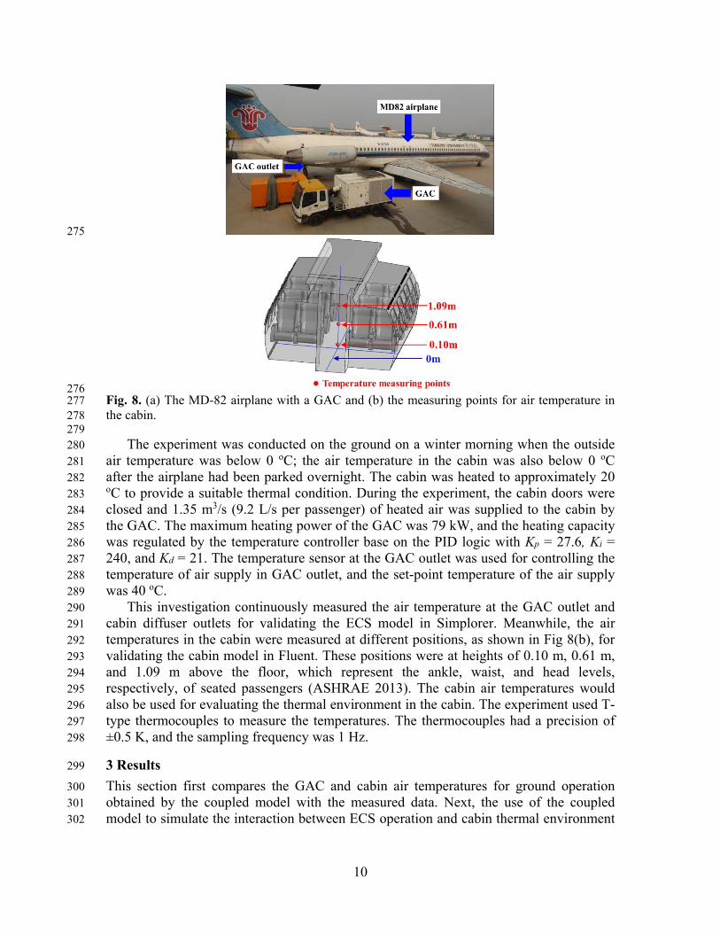
276 Fig. 8. (a) The MD-82 airplane with a GAC and (b) the measuring points for air temperature in 277 the cabin. 278 279

The experiment was conducted on the ground on a winter morning when the outside 280 air temperature was below 0 oC; the air temperature in the cabin was also below 0 oC 281 after the airplane had been parked overnight. The cabin was heated to approximately 20 282 oC to provide a suitable thermal condition. During the experiment, the cabin doors were 283 closed and 1.35 m3/s (9.2 L/s per passenger) of heated air was supplied to the cabin by 284 the GAC. The maximum heating power of the GAC was 79 kW, and the heating capacity 285 was regulated by the temperature controller base on the PID logic with Kp = 27.6, Ki = 286 240, and Kd = 21. The temperature sensor at the GAC outlet was used for controlling the 287 temperature of air supply in GAC outlet, and the set-point temperature of the air supply 288 was 40 oC. 289

This investigation continuously measured the air temperature at the GAC outlet and 290 cabin diffuser outlets for validating the ECS model in Simplorer. Meanwhile, the air 291 temperatures in the cabin were measured at different positions, as shown in Fig 8(b), for 292 validating the cabin model in Fluent. These positions were at heights of 0.10 m, 0.61 m, 293 and 1.09 m above the floor, which represent the ankle, waist, and head levels, 294 respectively, of seated passengers (ASHRAE 2013). The cabin air temperatures would 295 also be used for evaluating the thermal environment in the cabin. The experiment used T-296 type thermocouples to measure the temperatures. The thermocouples had a precision of 297 ±0.5 K, and the sampling frequency was 1 Hz. 298

3 Results 299

This section first compares the GAC and cabin air temperatures for ground operation 300 obtained by the coupled model with the measured data. Next, the use of the coupled 301 model to simulate the interaction between ECS operation and cabin thermal environment 302

11

for in-flight operation is discussed. Finally, this section presents an analysis of the impact 303 of ECS operation control on the cabin thermal environment. 304

3.1 Validation of the coupled simulation for ground operation 305

Fig. 9 compares the calculated air temperatures at the GAC outlet and the cabin air 306 diffuser outlets with the measured temperatures. The calculated results are in good 307 agreement with the experimental data. A small discrepancy was found at the GAC outlet 308 between 10 and 20 minutes after the GAC was turned on. The reason for this discrepancy 309 was that the actuation time via PID controller for the actuators in the GAC system was 310 different for the experiment than for the simulation model. Therefore, the temperature 311 calculated by the model was higher than the measured temperature, and the set-point 312 temperature was reached faster in the calculations. Since this small discrepancy should be 313 acceptable, the ECS model implemented in ANSYS Simplorer for ground conditions 314 performed as expected. 315

316

317 (a) (b) 318

Fig. 9. Comparison of the calculated GAC and cabin air temperatures with measured 319 temperatures during ground operation: (a) at the GAC outlet and (b) at the cabin diffuser outlets. 320 321

Fig. 10 compares the air temperatures in the cabin calculated by ANSYS Fluent with 322 the experimental data at the three positions shown in Fig. 8(b). The simulated air 323 temperatures agree well with the experimental data. The results show vertical temperature 324 stratification throughout the heating process. After 30 minutes, the air temperature at 325 head level reached 18.3 oC, which was sufficient for boarding (ASHRAE 2013). 326 Although the air temperature below head level was still low, passengers’ movements 327 during boarding would enhance the mixing of air. The aircraft requires more than 30 328 minutes to heat up its cabin as obviously seen in Figure 10. However, in this validation 329 experiment, the measurements were conducted for only 30 minutes because the external 330 air temperature and solar radiation conditions changed rapidly and unpredictably in the 331 winter morning. We were not allowed to take early measurements due to noise control on 332 the campus in the morning. When the winter clothing level is taken into account, the 333 thermal environment is capable of providing acceptable thermal comfort for passengers 334 and crew. 335

336

0 5 10 15 20 25 30-5

0

5

10

15

20

25

30

35

40

45

Tem

pera

ture

(oC

)

Heating time (min)

EXP-GAC outlet SIM-GAC outlet

0 5 10 15 20 25 30-5

0

5

10

15

20

25

30

35

40

45

Tem

pera

ture

(o C

)

Heating time (min)

EXP-cabin diffuser outlet SIM-cabin diffuser outlet

12

337 Fig. 10. Comparison of calculated air temperatures with experimental data in the cabin at heights 338 of 0.10 m, 0.61 m, and 1.09 m above the floor. 339

3.2 Coupling Simplorer and Fluent Simulation for In-flight Operation 340

The comparison of the air temperatures calculated by Simplorer and Fluent with the 341 corresponding experimental data confirmed the reliability of the model developed in this 342 study. This investigation further applied the model to a short flight of 3340 s to simulate 343 the interaction between the ECS and the cabin thermal environment. The flight consisted 344 of 4 minutes for taxiing from the terminal to the runway, 1 minute for takeoff from the 345 runway, 15 minutes for climbing to the cruising altitude of 10 km, 5 minutes for cruising, 346 20 minutes for descending, 40 seconds for landing, and 5 minutes for taxiing to the 347 terminal. Fig. 11 shows the flight altitude and cabin pressure schedule at different stages 348 of the flight. The rapid changes in ambient temperature and pressure during the flight 349 would have influenced the thermodynamic processes of the ECS and the boundary 350 conditions of the cabin. The ambient air temperature was assumed to be 0 oC on the 351 ground and then changed at a rate of -6.5 oC/km altitude. The cabin air temperature was 352 initiated at 23 oC. Meanwhile, the cabin air temperature should be maintained at 23 oC 353 during the entire flight process (ASHRAE 2013) thereby the set temperature in PID 354 controller was 23 oC as well. 355

356

357 Fig. 11. The aircraft altitude and cabin pressure during the flight. 358

359 Throughout the entire flight process, the aircraft ECS was regulated to maintain a 360

stable thermal environment in the cabin. Fig. 12(a) compares the cabin air temperature at 361 the feedback point during the flight with the set-point temperature. The temperature at the 362

0 3 6 9 12 15 18 21 24 27 30

0

3

6

9

12

15

18

21

24

Tem

per

atu

re (

o C)

Heating time (min)

EXP-0.10m EXP-0.61m EXP-1.09m SIM-0.10m SIM-0.61m SIM-1.09m

0 500 1000 1500 2000 2500 3000

0

2

4

6

8

10

12

Flight altitude Cabin pressure

Flight time (s)

Flig

ht a

ltitu

de (

km)

0.0

0.2

0.4

0.6

0.8

1.0

1.2

Cab

in p

ress

ure

(at

m)

13

feedback point was lower than the set-point value during the climbing process and higher 363 than the set-point value during the descending process. This difference is due to the fact 364 that the ambient temperature decreased gradually during the climbing process and 365 increased gradually descent. However, with the PID controller the temperature at the 366 feedback point was stable within a range during the entire flight. The temperature 367 difference between the feedback point and set point was smaller than ±0.6 K, which was 368 within the ±1.1 K required by the ASHRAE standard (ASHRAE 2013). 369

370 (a) (b) 371

Fig. 12. (a) The controlled cabin air temperature and (b) the bypass flow ratio of the bleed air in 372 the ECS and the temperature of the supply air to the cabin. 373 374

Fig 12 (b) shows the bypass flow ratio of the total bleed air in the ECS and the 375 temperature of the supply air to the cabin during the entire flight process. As shown in 376 Fig. 3, the bypass flow ratio was controlled directly by the PID controller through the 377 flow valve. At the beginning of the process, the cabin air temperature changed slightly, 378 and thus the bypass flow ratio had a small change as well. The bypass flow ratio then 379 increased during the climbing stage because of the increasing thermal load in the cabin, 380 and the reverse trend can be observed in the descending stage. The maximum bypass 381 flow ratio was reached in the cruising stage because the thermal load in the cabin was the 382 highest while the outside air temperature was the lowest. The supply air temperature 383 increased with the increase in bypass flow ratio, and thus the highest supply air 384 temperature was likewise found in the cruising stage. However, the supply air 385 temperature fluctuated to a greater extent than the bypass flow ratio because the supply 386 air temperature was also influenced by the air temperature at the turbine outlet and the 387 return air temperature, which would have changed with the flight stage and time. The 388 mean supply air temperature in the cruising state was about 22.5 oC, which is lower than 389 the cabin air temperature of 23 oC, because more heat was released by the 12 manikins 390 than was loss through the walls. The air temperatures and bypass flow ratio simulated by 391 Simplorer indicate excellent control. 392

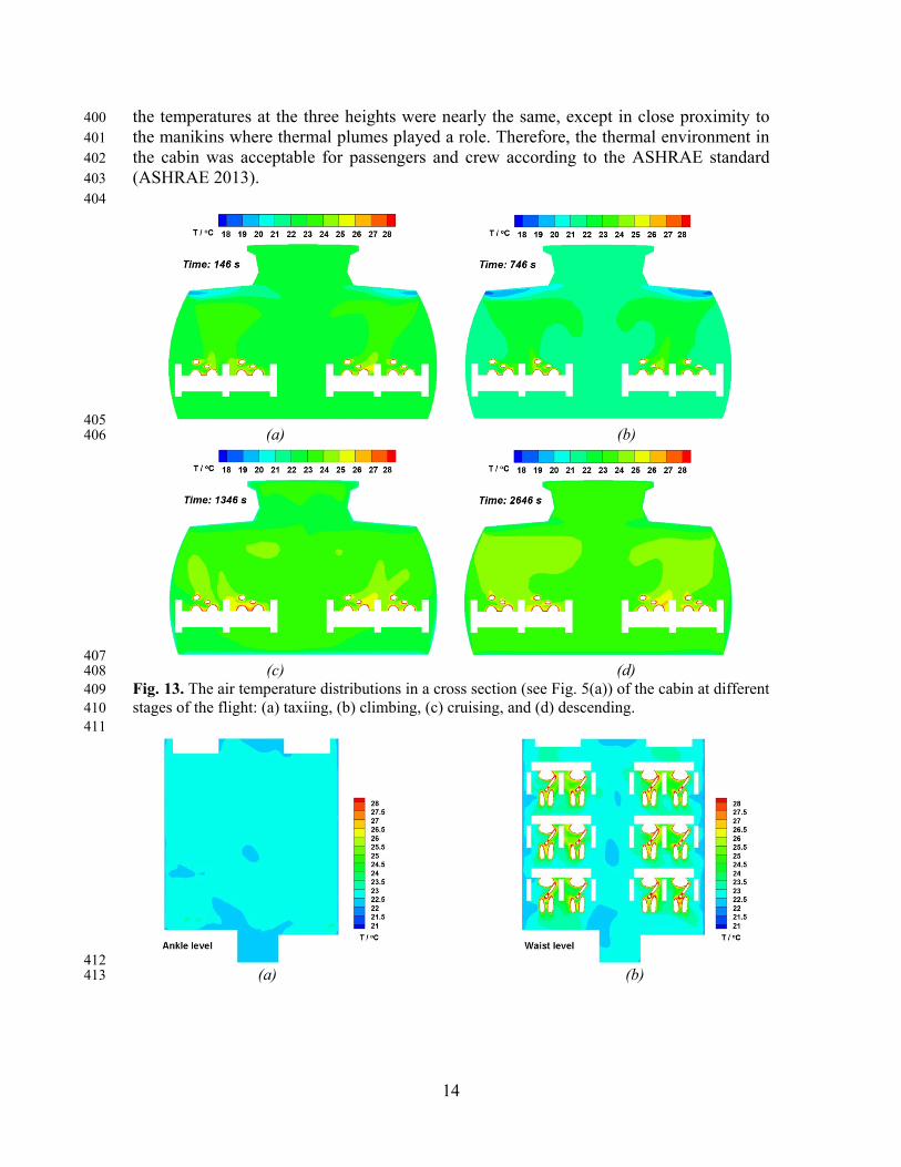
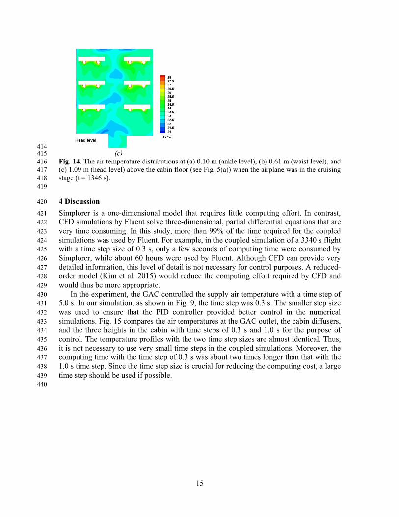
Figs. 13 and 14 show the air temperature distributions in the cabin as calculated by 393 Fluent. Fig. 13 depicts the distributions in a cross section (see Fig. 5(a)) at the taxiing, 394 climbing, cruising, and descending stages. The distributions were relatively uniform at 395 the climbing, cruising, and descending stages, when the flow was relatively stable and 396 mixing was good. Fig. 14 shows the temperature distributions at cruising altitude (t = 397 1346 s) at heights of 0.10 m, 0.61 m, and 1.09 m above the floor (see Fig. 5(a)), which 398 represent the ankle, waist, and head levels, respectively. Because of mixing ventilation, 399

0 500 1000 1500 2000 2500 300021

22

23

24

25

Tem

pera

ture

(o C

)

Flight time (s)

Tf

Tset

0 500 1000 1500 2000 2500 300010

15

20

25

30

35

Qb

Ts

Flight time (s)B

ypas

s flo

w r

atio

(%

)

16

18

20

22

24

Tem

pera

ture

(oC

)

14

the temperatures at the three heights were nearly the same, except in close proximity to 400 the manikins where thermal plumes played a role. Therefore, the thermal environment in 401 the cabin was acceptable for passengers and crew according to the ASHRAE standard 402 (ASHRAE 2013). 403

404

405 (a) (b) 406

407 (c) (d) 408

Fig. 13. The air temperature distributions in a cross section (see Fig. 5(a)) of the cabin at different 409 stages of the flight: (a) taxiing, (b) climbing, (c) cruising, and (d) descending. 410 411

412 (a) (b) 413

15

414 (c) 415

Fig. 14. The air temperature distributions at (a) 0.10 m (ankle level), (b) 0.61 m (waist level), and 416 (c) 1.09 m (head level) above the cabin floor (see Fig. 5(a)) when the airplane was in the cruising 417 stage (t = 1346 s). 418 419

4 Discussion 420

Simplorer is a one-dimensional model that requires little computing effort. In contrast, 421 CFD simulations by Fluent solve three-dimensional, partial differential equations that are 422 very time consuming. In this study, more than 99% of the time required for the coupled 423 simulations was used by Fluent. For example, in the coupled simulation of a 3340 s flight 424 with a time step size of 0.3 s, only a few seconds of computing time were consumed by 425 Simplorer, while about 60 hours were used by Fluent. Although CFD can provide very 426 detailed information, this level of detail is not necessary for control purposes. A reduced-427 order model (Kim et al. 2015) would reduce the computing effort required by CFD and 428 would thus be more appropriate. 429

In the experiment, the GAC controlled the supply air temperature with a time step of 430 5.0 s. In our simulation, as shown in Fig. 9, the time step was 0.3 s. The smaller step size 431 was used to ensure that the PID controller provided better control in the numerical 432 simulations. Fig. 15 compares the air temperatures at the GAC outlet, the cabin diffusers, 433 and the three heights in the cabin with time steps of 0.3 s and 1.0 s for the purpose of 434 control. The temperature profiles with the two time step sizes are almost identical. Thus, 435 it is not necessary to use very small time steps in the coupled simulations. Moreover, the 436 computing time with the time step of 0.3 s was about two times longer than that with the 437 1.0 s time step. Since the time step size is crucial for reducing the computing cost, a large 438 time step should be used if possible. 439

440

16

441 (a) (b) 442

443 (c) 444

Fig. 15. The effects of time step size in the coupled model on the air temperature (a) at the GAC 445 outlet, (b) at the cabin diffusers, and (c) at different heights in the cabin. 446

447

5 Conclusions 448

This investigation developed a model for ECS operation on the ground and in flight in 449 ANSYS Simplorer. The thermal environment in an airplane cabin was simulated by 450 ANSYS Fluent. Coupling of Simplorer and Fluent makes it possible to simulate transient 451 control of the ECS and the cabin environment. The simulated air temperatures at various 452 locations were compared with the experimental data obtained in an MD-82 aircraft cabin 453 on ground. The study led to the following conclusions: 454

The simulated air temperatures at the outlets of the GAC and cabin air diffusers agree 455 with the measured data obtained from an MD-82 airplane and a GAC in ground 456 operation. This comparison implied that the coupled simulations were reliable for 457 simulating the interaction between the indoor thermal environment and the ECS. 458

Coupled simulations were also conducted for in-flight operation. The results show 459 that the PID controller used in the ECS can effectively maintain the cabin air temperature 460 at a level that provides acceptable thermal comfort for passengers and crew members. 461

The CFD simulations of thermal environment by Fluent were very time consuming. 462 To reduce computing costs, the time step size used in the simulations could be increased 463 without compromising accuracy. 464

Nevertheless, this study provided useful information for numerically testing the 465 performance of ECS and evaluating the thermal environment in a cabin during aircraft 466 design. 467

0 5 10 15 20 25 30-5

0

5

10

15

20

25

30

35

40

45

Tem

pera

ture

(oC

)

Heating time (min)

EXP SIM-0.3s SIM-1.0s

0 5 10 15 20 25 30-5

0

5

10

15

20

25

30

35

40

45

Tem

pera

ture

(oC

)

Heating time (min)

EXP SIM-0.3s SIM-1.0s

0 5 10 15 20 25 30

0

4

8

12

16

20

24

Tem

pera

ture

(o C

)

Time (min)

EXP-0.10m EXP-0.61m EXP-1.09m SIM-0.10m-0.3s SIM-0.61m-0.3s SIM-1.09m-0.3s SIM-0.10m-1.0s SIM-0.61m-1.0s SIM-1.09m-1.0s

17

468

References 469

ANSYS (2014). ANSYS Fluent Version 15.0. ANSYS, Inc. 470 ANSYS (2014a). ANSYS Simplorer Version 15.0. ANSYS, Inc. 471 ASHRAE Handbook- HVAC Application (2011). American Society of Heating, 472

Refrigerating and Air-Conditioning Engineers, Inc. (www.ashrae.org). 473 ASHRAE (2013). Air Quality within Commercial Aircraft. In: ANSI/ASHRAE Standard 474

161-2013. Atlanta, USA: ASHRAE. 475 Chen C, Lin C.H, Long Z, Chen Q (2014). Predicting transient particle transport in 476

enclosed environments with the combined CFD and Markov chain method. Indoor 477 Air, 24: 81-92. 478

Duan R, Liu W, Xu L, Huang Y, Shen X, Lin C.H, Liu J, Chen Q, Sasanapuri B (2015). 479 Mesh type and number for CFD simulations of air distribution in an aircraft cabin. 480 Numerical Heat Transfer, Part B: Fundamentals, 67(6): 489-506. 481

Eichler J (1975). Simulation study of an aircraft's environmental control system dynamic 482 response. Journal of Aircraft, 12(10): 757-758. 483

Hofman J.M.A (2003). Control–fluid interaction in air-conditioned aircraft cabins: A 484 demonstration of stability analysis for partitioned dynamical systems. Computer 485 Methods in Applied Mechanics and Engineering, 192(44): 4947-4963. 486

Huang Y, Li J, Li B, Duan R, Lin C.H, Liu J, Shen X, Chen Q (2015). A method to 487 optimize sampling locations for measuring indoor air distributions. Atmospheric 488 Environment, 102: 355-365. 489

Hu X, You X (2015). Determination of the optimal control parameter range of air supply 490 in an aircraft cabin. Building Simulation, 8(4): 465-476. 491

Kim D, Braun J.E, Cliff E.M, Borggaard J.T (2015). Development, validation and 492 application of a coupled reduced-order CFD model for building control applications. 493 Building and Environment, 93(2): 97-111. 494

Leo T.J, Pérez-Grande I (2005). A thermoeconomic analysis of a commercial aircraft 495 environmental control system. Applied Thermal Engineering, 25: 309-25. 496

Li M, Zhao B, Tu J, Yan Y (2015). Study on the carbon dioxide lockup phenomenon in 497 aircraft cabin by computational fluid dynamics. Building Simulation, 8(4): 431-441. 498

Liu W, Chen Q (2015). Optimal air distribution design in enclosed spaces using an 499 adjoint method. Inverse Problems in Science and Engineering, 23(5): 760-779. 500

Liu W, Mazumdar S, Zhang Z, Poussou S.B, Liu J, Lin C. H, Chen Q (2012b). State-of-501 the-art methods for studying air distributions in commercial airliner cabins. Building 502 and Environment, 47: 5-12. 503

Liu W, Wen J, Chao J, Yin W, Shen C, Lai D, Lin C.H, Liu J, Sun H, Chen Q (2012a). 504 Accurate and high-resolution boundary conditions and flow fields in the first-class 505 cabin of an MD-82 commercial airliner. Atmospheric Environment, 56: 33-44. 506

Mazumdar S, Long Z, Chen Q (2014). A coupled CFD and analytical model to simulate 507 airborne contaminant transmission in cabins. Indoor and Built Environment, 23: 946-508 954. 509

Ordonez J.C, Bejan A (2003). Minimum power requirement for environmental control of 510 aircraft. Energy, 28: 1183-202. 511

18

Pérez-Grande I, Leo T.J (2002). Optimization of a commercial aircraft environmental 512 control system. Applied thermal engineering, 22(17): 1885-1904. 513

Poussou S, Mazumdar S, Plesniak M.W, Sojka P, Chen Q (2010). Flow and contaminant 514 transport in an airliner cabin induced by a moving body: Scale model experiments 515 and CFD predictions. Atmospheric Environment, 44(24): 2830-2839. 516

World Bank Group (Ed.) (2015). 2015 World Development Indicators. World Bank 517 Publications. 518

Zhang Z, Chen X, Mazumdar S, Zhang T, Chen Q (2009). Experimental and numerical 519 investigation of airflow and contaminant transport in an airliner cabin mockup. 520 Building and Environment, 44(1): 85-94. 521

Zhao H, Hou Y, Zhu Y, Chen L, Chen S (2009). Experimental study on the performance 522 of an aircraft environmental control system. Applied Thermal Engineering, 29(16): 523 3284-3288. 524