Modeling Challenges

At High Latitudes

Judith Curry

Georgia Institute of Technology

Physical Process Parameterizations

Radiative transfer

Surface turbulent fluxes

Cloudy boundary layer

Cloud microphysics

Sea ice thermodynamics and optics

Physical Process Parameterizations

Radiative transfer

Surface turbulent fluxes

Cloudy boundary layer

Cloud microphysics

Sea ice thermodynamics and optics

Radiative Transfer

The clear-sky radiative transfer is essentially solved

• major breakthrough from SHEBA (“dirty window”)

Remaining issues:

• cloud overlap issue (CloudSat and Calipso should help)

• consistency between microphysics code and r.t. code in

specifying cloud optical properties

• correct handling of the highly reflecting surface

• 3D radiative transfer not a big issue in the polar regions

Surface turbulent fluxes

Lead

plume

Fluxes over multi-year ice are small; uncertainty in

role of gravity waves in surface fluxes

Fluxes over open leads can be very

large during winter, ~500 W/m2

NO DATA !

Boundary Layer Parameterizations

Existing B.L. parameterizations work poorly in the Arctic,

owing to:

! Static stability and strong temperature inversions

! Persistent negative surface heat fluxes

! Large-scale subsidence

! Mixed phase and crystalline clouds

Result in

• Incorrect vertical profiles of T, q, u

• Incorrect clouds

• incorrect surface fluxes

The main issue is not lack of observations

(other than leads)

Local schemes match LES most closely for temperature

SHEBA (Jan): Clear stable b.l.

Ph.D. Thesis, Jeff Mirocha

Main problem with nonlocal schemes is diagnosis of b.l. height

SHEBA (Jan): Clear stable b.l.

Ph.D. Thesis, Jeff Mirocha

All perform worse in presence of subsidence

SHEBA (Jan): Clear stable b.l.

Ph.D. Thesis, Jeff Mirocha

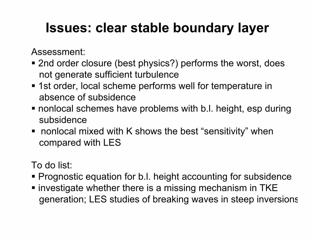
Issues: clear stable boundary layer

Assessment:

! 2nd order closure (best physics?) performs the worst, does

not generate sufficient turbulence

! 1st order, local scheme performs well for temperature in

absence of subsidence

! nonlocal schemes have problems with b.l. height, esp during

subsidence

! nonlocal mixed with K shows the best “sensitivity” when

compared with LES

To do list:

! Prognostic equation for b.l. height accounting for subsidence

! investigate whether there is a missing mechanism in TKE

generation; LES studies of breaking waves in steep inversions

Cloudy Boundary Layer

Main problems:

! (stable b.l. issues)

! Thermal b.l. different from momentum b.l.

! Thermodynamics for b.l. crystalline and

mixed phase clouds

Representation of Arctic Clouds in Models

• Atmospheric Model

Intercomparison Project (AMIPII).

• Annual cycle is vaguely captured,

though several are out of phase.

• Large variability between models.

From Walsh et al. (2002)

Possible reasons for poor simulations

of Arctic clouds

Poor large scale dynamical fields

Inadequate boundary layer parameterizations

Incorrect surface temperature and surface state

"Inadequate cloud microphysical parameterizations

Inadequate vertical resolution

Etc.

Arctic cloud microphysics:

cloud phase is the dominant issue

• At -30C, more than half the clouds have liquid

• Cloud phase has a substantial impact on radiative fluxes andprecipitation

Cloud Microphysical Models

A set of prognostic equations for:• Cloud drops• Ice crystals• Rain drops• Snow• Graupel

Bin resolving microphysics (specifies size spectra)

Bulk microphysics- Single moment (species mixing ratio)- Dual moment (+ particle concentration)

Microphysical elements that need parameterizing:• Liquid drop nucleation• Ice particle nucleation• Diffusional growth• Fall speed• Liquid droplet size spectra• Ice crystal size spectra• Particle collection and aggregation

Interfaces with model dynamics and thermodynamics:• Large-scale advective processes• Subgrid-scale supersaturation fluctuations

Arctic mixed-phase stratiform clouds

(AMPS)

•Often persist continuously for days or even weeks.

SHEBA cloud phase and LWP retrievals, May 4-8, 1998 (NOAA ETL).

Case Description

• The cloud layer was mixed-phase near cloud top, with

continuous light snowfall reaching the surface, and occasionally

surmounted by upper-level ice clouds.

Green – All-IceYellow – Mixed-Phase

Cloud Classification

Cloud Optical Depth

Courtesy of NOAA/ETL

May 4, 1998 May 5, 1998

• A two-moment scheme (predicting both mass and number

concentration) can produce long-lived mixed-phase clouds

at T ~ -21 C if droplet freezing is assumed to be the

dominant ice nucleation mechanism rather than deposition

nucleation

LWC

IWC

IWC

IWC

Two-moment scheme One-moment/quasi-one-moment schemes

Results for SHEBA grid cell (May 4-5, 1998), MM5 mesoscale simulations

(dx=20 km). From Morrison and Pinto (2006).

How does the modeled cloud layer compare with observations?

Retrieved liquid boundaries and MMCR reflectivity at SHEBA (top) and modeledliquid boundaries and ice water content (bottom) for CON run.

Why does the Morrison et al. scheme predict mixed-phase

clouds, while Reisner1/Reisner2 (single moment) predict all-

ice clouds?

• Reisner1 and Reisner2 (and most other microphysics

schemes) assume a continuous supply of ice nuclei

• The diagnosed snow number concentration is ~ 6 times

larger in Reisner1 and Reisner2 than predicted by the

Morrison et al. scheme.

• High production of ice/snow particles depletes liquid water

by the Bergeron-Findeisen process.

Model Description• Polar NCAR/PSU Fifth-Generation Mesoscale Model (MM5) version 3.6

(Bromwich et al., 2001; Cassano et al. 2001).

Location of the outer (D1) andinner (D2) model domains.

SHEBA

# Results for the inner domain will be shown.

• Mixed-phase rather than all-ice clouds result in overall warming of the surface

due to an increase in the downwelling longwave radiative flux.

• Strong cloud-top radiative cooling (~ 50 K/day) and surface warming induced

by the mixed-phase cloud result in a deep, surface-based, well-mixed BL.

Observed and modeled sea ice surfacetemperature (below) and potentialtemperature profiles (right) for the

SHEBA grid.

Reisner1/Reisner2

Baseline

ObservedObserved

Baseline

Reisner1/Reisner2

• Differences in surface temperature and near-surface stability induced by the mixed-

phase cloud result in a much larger surface turbulent flux of water vapor than in

Reisner1/Reisner2. This surface flux feeds moisture into the mixed-phase cloud and

balances the increased precipitation flux.

•

Cloud Glaciated Sensible Flux

Latent Flux

Observed turbulent near-surfacelatent and sensible heat fluxes.Note reduction to negative valuesduring the brief period that thecloud was glaciated.

•Diabatic processes induced by mixed-phase rather than all-ice clouds result in

higher surface pressure (up to 1 mb) and increased low-level subsidence.

• The development of mesoscale features (banding of vertical velocity and

surface pressure differences parallel to the geostrophic flow) may be due to

negative potential vorticity and symmetric instability circulations induced by

diabatic mixed-phase cloud processes.

Surface pressure difference (baseline - Reisner1)at end of simulation (0000 UTC May 6) (mb).

Low-level vertical velocity difference (baseline -Reisner1) at end of simulation (0000 UTC May 6)

(cm/s).

* SHEBA

Mixed Phase Cloud Summary

• Mixed-phase clouds dominate cloud fraction over the ArcticOcean for most of the year.

• Arctic M-P clouds are difficult to simulate, and most modelsincorrectly represent them as entirely crystalline.

• Parameterizations basing cloud phase on temperature do nothave sufficient degrees of freedom and current paramsintroduce bias of too much ice

• In models with separate prognostic variables for ice andliquid, simulated M-P clouds are highly sensitive to the icecrystal concentration and mode of nucleation.

• Heterogeneous ice nucleation is poorly understood. Thedominant mode in Arctic mixed phase clouds appears to bedroplet freezing (mainly contact; impact of immersionunknown). Note: deliquescence freezing is the main modemeasured in field missions

Sea Ice Modeling

Sea ice feedbacks are complex:internal sea ice processesinteractions with the local atmosphere and oceaninteractions with global processes

Current sea ice models and parameterized interactionswith the atmosphere and ocean are likely to beinadequate at simulating the climate in an altered sea iceregime.

Improved parameterizations related to sea ice are notmaking it into climate models.

But what about SHEBA?

SHEBA observations:

#thermodynamical and optical properties and processes

#exchanges at ice/atm and ice/ocean interfaces

8 years after the SHEBA field experiment, none of theseobservations have influenced new parameterizations in sea icemodels used in GCMs

Needed Improvements to Sea Ice Models

•Spectral radiative transfer: surface albedo, transmissionthrough snow, sea ice, upper ocean. !

•Explicit melt ponds: albedo, latent heat, salinity effects !

•Snow:nonlinear conduction, metamorphism, redistribution !

•Ice age: optics, thermal conductivity, specific heat, etc. !

•Formation of snow/ice

•Frazil ice formation

•Ice deformation: brine rejection;enhanced decay of ridgedice

•Lead width distribution: lateral melting, turbulent fluxes

•Ice/ocean turbulent flux for ice thickness distribution !

•Fast ice: detailed ocean bathymetry,granular rheology

! Good data available from SHEBA

Impediments to improving sea icecomponent of climate models

Sea ice modeling community focused on large scale dynamicalice/ocean interactions.

Models are currently highly tuned; adding a new/betterparameterization is likely to make the model simulations worse.

There is no hierarchical modeling strategy to develop and evaluatenew sea ice parameterizations: needed to assess how important agiven parameterization is (no analogy to GCSS, ARM in the sea icemodelling world).

Inadequate funding base; sea ice scientists favor field measurementsin the review process; people are leaving the field.

Observations/process studies and parameterization ideas are NOTpresently the limiting factor in progress

What is needed for a parameterization to be successful:

1. Theory and detailed process modeling to focus on specific param elements

2. Conduct simulations using the process models for the entire relevant range of

thermodynamical and dynamical conditions; evaluate using obs !

3. Develop new param, guided by theory and statistics, from process model

simulations

4. Test new param in CRMs, SCMs (including linkages to other parameterizations);

evaluate using obs !

5. Conduct sensitivity studies to see if the complexity of new param can be reduced

(or needs to be increased)

6. Incorporate new param into a mesoscale model, for domain < RoD (driven by

lateral boundaries, not sensitive to initial conditions); evaluate using obs !

7. Examine new param in mesoscale model for larger domain simulations

8. Incorporate new param into GCM, assess impact of param on the model climate;

evaluate using obs !

9. Conduct GCM sensitivity studies to understand how param alters sensitivity

! Return to #1 or proceed forward

Summary of parameterization issuesMostly solved issues:

• clear sky radiative transfer • surface turbulent fluxes over ice/snow

Issues with major progress expected in short term• cloud microphysics and interactions with aerosols

Issues limited by observations:• turbulent fluxes over leads• new ice formation, coastal sea ice, ridges

Issues limited by understanding:• stable boundary layer• cloud-turbulence interactions

• heterogeneous ice nucleation

Issues limited by community barriers:• sea ice thermodynamics and optics• linkages between parameterizations