International Journal of the Physical Sciences Vol. 6(18), pp. 4388-4404, 9 September, 2011 Available online at http://www.academicjournals.org/IJPS ISSN 1992 - 1950 ©2011 Academic Journals

Full Length Research Paper

Modeling and simulation of maglev train-guideway-tunnel-soil system for vibration

Jianwei Wang1,2, Xianlong Jin1,2* and Yuan Cao1,2

1State Key Lab of Mechanical System and Vibration, Shanghai Jiao Tong University, Shanghai 200240, China.

2School of Mechanical Engineering, Shanghai Jiao Tong University, Shanghai 200240, China.

Accepted 30 June, 2011

A maglev train-guideway-tunnel-soil coupling system model is developed to study the wave propagation problem caused by high speed electromagnetic suspension (EMS) maglev train travelling through tunnel. The maglev train is simulated by multi-bodies, which takes the rigid body characteristics of the body-bogie-magnet system into account. The guideway-tunnel-soil system is simulated by 3D finite elements, and the unbounded domain is simulated by Perfect match layer (PML). The interaction between maglev train and guideway is simulated by the equivalent spring/damping magnetic force model. The dynamic factor of guideway is well estimated comparing with the German design guideline. A certain parameters related to the maglev train, tunnel and soil are considered to investigate the vibration of tunnel and ground surface. Key words: Maglev train, finite element, perfect match layer (PML), tunnel, wave propagation.

INTRODUCTION The maglev train replaces wheels by electromagnets and levitates on the guideway, producing propulsion force electromechanically without any contact. This non-contact maglev system results numerous advantages comparing to the conventional wheel-rail system: High speed, efficient acceleration and braking, low main-tenance and environmentally friendly (no direct emission, low noise and energy consumption) etc (Lee et al., 2006), which is highly competitive for public transportation. With the development of the maglev transportation system, tunnel needs to be built when maglev train travels through large river or mountain, and other sensitive or densely populated areas. Most of the research on maglev technology has been conducted in the past several decades. However, these studies are mostly focused on the dynamic interaction of maglev train/guideway system, no research referred to the tunnel-soil system had been conducted (Shi et al., 2007; Hägele and Dignath, 2009; Lee et al., 2009). But the dynamic problem between the conventional train and tunnel-soil systems had been studied by many researchers, in which the numerical *Corresponding author. E-mail: jxlong@sjtu.edu.cn. Tel: +86 21 34206099. Fax: +86 21 34206338.

methods have emerged as an effective tool for solving this problem. Gardien and Stuit (2003) proposed a modular finite element modeling method for analyzing vibrations generated by trains running through the tunnels. Sheng et al. (2006) studies the ground-born vibration using the wavenumber finite/boundary element method. Andersen and Jones (2006) studied the vibration transmission from the tunnel to the ground using a coupled finite-boundary element scheme. Yang et al. (2008) studied the soil vibration problems caused by underground moving trains using the 2.5D finite/infinite element approach. In the 2.5D approach, the material and geometric properties is considered as constant along the load-moving direction; only the profile of the half-space normal to the load-moving direction need be considered; a 3D response can be obtained from the 2D profile by the Fourier transformation technique. Gupta et al. (2009) studied the vibrations induced by underground trains using coupled periodic FE-BE model for several tunnels. In these studies, the finite element method has been proved to be an effective method, where artificial boundary, boundary element and infinite element are typical approaches to simulation the infinite domain. A 3D maglev train-guideway-tunnel-soil model is presented in this paper to study the dynamic response due to the high speed EMS maglev train travelling in a tunnel, in which the

train is modeled by multi-rigid bodies, the guideway, tunnel and soil are modeled by finite elements with perfect match layer (PML) artificial boundary, and the magnetic force between maglev vehicle and guideway is modeled by linear spring-damping system. METHODOLOGY Rigid body algorithm in finite element program

The finite element method has been proved to be an effective method for the underground train induced vibration problem. In order to take the rigid body characteristics of the body-bogie-magnet system into account, the rigid body algorithm in finite element program is needed. The equations of motion for a rigid body are given by Benson and Hallquist (1986):

cm xi i

ij j ijk j kl l i

MX FJ e J Fωω ω ω =

+ =

&&

& (1)

where M is the diagonal mass matrix, J is the inertia tensor,

cmX is the location of the mass center, ω is the angular velocity

of the body, ijk

e is the Levi-Civita permutation tensor and

xF , Fω are the generalized forces and torques, respectively. A rigid body in finite element structural dynamics program is defined using finite element mesh by specifying that all the elements in a region are rigid. Thus, the central issues associated with implementing Equation (1) include (Benson and Hallquist, 1986):

1. Calculate M and J from the mesh defining the body: In many

of the equations that follow, summations are performed over all the nodes associated with all the elements in a rigid body, and these

special summations are denoted asRB

α∑ .

The rigid body mass is calculated by performing a summation:

RB

M mαα=∑ (2)

where the subscript α indicates the node that associated with the

elements in a rigid body and mα is the mass of node α .

The inertia tensor is also calculated by performing a summation:

( )2RB

ij ij i jJ m x x xα α α ααδ= − ∑ (3)

where cmx x Xα α= − .

2. Calculate xF and Fω: The forces and torques are found by

summing over the nodes:

RBx

i iRB

i ijk j k

F f

F e x f

αα

ωα αα

=

=

∑∑

(4)

The summations automatically accounts for all of the forces (concentrated loads, gravity, impact forces, surface traction, interface forces etc.). 3. Update displacements, velocities and

Wang et al. 4389 inertia tensor of the rigid body: The displacement of the rigid body is measured from the mass center to eliminate the coupling between the translational and rotational momentum equations. The initialized location of the mass center is calculated by:

( )RBcmi i

X m x Mα αα= ∑ (5)

The initial velocities of the nodes are calculated for a rigid body from:

( )cmi i ijk j kn j

x X e A xα αω θ= +&& (6)

where A is the transformation from the rotated reference

configuration to the global coordinate frame,θ is the measure of

the rotation of the body, ω is the angular velocity of the body in the

global coordinate frame. At the initial time, A is the identity transformation, and the reference configuration is assumed to be co-aligned with the global reference frame.

After calculating the rigid body accelerations from Equation (1), the rigid body velocities are updated by the central difference method. The inertia tensor must be transformed each time step based on the incremental rotations:

( ) ( ) ( ) ( )1ij n km nik jmJ t A A J tθ θ+ = ∆ ∆ (7)

The incremental rotation matrix is calculated using the Hughes-Winget algorithm (Hughes and Winget, 1980).The coordinates and velocities of the nodes of the rigid body are updated:

( ) ( ) ( ) ( )( ) ( )( )( ) ( )1 1 1cm cm

i n i n i n i n n ij j nijx t x t X t X t A t x tα α αθ δ+ + += + − + ∆ − (8)

( ) ( ) ( )1/2 1i n i n i n nx t x t x t tα α α+ += − ∆ & (9)

where ( ) ( ) ( )cmi n i n i n

x t x t X tα α= − .

PML artificial boundary Using the finite element method to simulate the wave propagation in the infinite domain, an artificial boundary that absorbs outgoing waves for the modeling of the unbounded domain is required. Boundary element method typically gives fully populated and non symmetrical matrices, which means a high storage and computation cost. Although compression techniques can be used to ameliorate these problems, the complexity is highly added and the success-rate depends heavily on the nature of the problem being solved and the geometry involved. Appling infinite element to colored wave propagation problem, where compression, shear, Rayleigh and Love waves are present, the decay parameter for each wave type is necessary and the parameters describing the distribution of energy among different waves must be assigned. These parameters must be determined empirically or resort to existing analytical solutions. It is difficult that so many uncertain parameters need to be determined in this study. Perfect match layer (PML) is a wave absorbing layer that placed adjacent to a truncated model of an infinite domain. By applying a particular form of the coordinate stretch (in terms of appropriate attenuation function) to the elastic wave equation, the PML can perfectly attenuate all non-tangential angles-of-incidence and all non-zero frequencies outgoing waves

4390 Int. J. Phys. Sci. and reflected waves back toward the truncated domain with arbitrarily small amplitude (Ma and Liu, 2006). The storage and computation cost is small, and the parameters could be easily determined. The governing equations of a PML are most naturally defined in the frequency domain, by assuming a harmonic time dependence of the displacement, stress and strain,

e.g. ( ) ( ) ( ), expu x t u x i tω= , where ω is the frequency of

excitation. Let a three-dimensional space be defined by the

coordinate system { }ix , with respect to an orthonormal basis

{ }ie . The PML is defined by the coordinate system { }'ix , with

respect to another orthonormal basis{ }'ie . The two bases are

related by the rotation-of-basis matrix Q , with components

':ij i jQ e e= � . By applying mutually independent nowhere-zero,

continuous, complex-valued stretching function i

λ to each of the

coordinates { }'ix , as well as the coordinate transforming, the

governing frequency-domain equations for a PML in the

basis{ }ie can be obtained (Basu and Chopra, 2003).

( ) ( )

( )

' 2 '

1

2

i i i i

i i

T

x x u

C

u u

σ λ ω ρ λ

σ ε

ε

∇ Λ = −

=

= ∇ Λ + ∇ Λ

∏ ∏�

(10)

where ' TQ QΛ = Λ ,

( ) ( ) ( )( )' ' ' '1 1 2 2 3 31/ ,1/ ,1/diag x x xλ λ λΛ = and C is the

elastic constitutive tensor. The stretching function is assumed with the form (no summation)

(Basu and Chopra, 2004):

( ) ( ) ( ) ( )' ' '1

: 1 pei i i i i i s

x f x f x c Li

λω = + + × (11)

wheres

c is the shear wave speed and L is the characteristic length

of the system; a convenient choice for L is the depth of the PML.

The functions ei

f and p

if serve to attenuate evanescent waves

and propagating waves, respectively. Substituting Equation (11) into Equation (10) and applying the inverse Fourier transform to the resultant to obtain the time-domain equations of the 3D elastic PML (Basu, 2009):

( ) ( ) ( ) ( )

( ) ( ) ( ) ( )

( ) ( ) ( ) ( )

2 3

1 1

2 2

ee ep ppM s C s K s H

T T T Te e p e e p p p

T T T Te e p p

F F F f u c L f u c L f u c L f u

C

F F F F F F F EF

F u u F F u u F

σ ρ ρ ρ ρσ ε

ε ε ε

∇ + Σ + Σ = + + +=

+ + +

= ∇ + ∇ + ∇ + ∇

% && && && &&�

&

& &

(12)

where

0:

t

U udτ= ∫ ,0

:t

E dε τ= ∫ ,0

:t

dσ τΣ = ∫ ,0

:t

dτΣ = Σ∫% (13)

( )( )

( )( ) ( )( ) ( )

( )( ) ( ) ( )

( )( )

'

' ' '

' ' '

'

: 1

: 1 1

: 1

: 1

eM i i

i

pe eC i i j j k k

i j k

p peK i i j j k k

i j kp

H i i

i

f f x

f f x f x f x

f f x f x f x

f f x

≠ ≠

≠ ≠

= +

= + +

= +

= +

∏

∑

∑

∏

(14)

and 'e e TF QF Q= , 'p p TF QF Q= , 'ee ee TF QF Q= ,

'ep ep TF QF Q= , 'pp pp TF QF Q=

(15)

with

( ) ( ) ( )( )( ) ( ) ( )( ) ( )

( )( ) ( )( ) ( )

' ' ' '1 1 2 2 3 3

' ' ' '1 1 2 2 3 3

'23 13 12

'23 13 12

2'

23 13 12

: 1 ,1 ,1

: , ,

: , ,

: , ,

: , ,

e e e e

p p pps

ee ee ee ee

ep ep epeps

pp pp pppps

F diag f x f x f x

F diag f x f x f x c L

F diag f f f

F diag f f f c L

F diag f f f c L

= + + +

= ×

=

= ×

= ×

(16)

where eeij

f , etc. are defined as (no summation)

( )( ) ( )( )( )( ) ( ) ( )( ) ( )

( ) ( )

' '

' ' ' '

' '

: 1 1

: 1 1

:

ee e eij i i j j

ep p pe eij i i j j j j i i

pp p p

ij i i j j

f f x f x

f f x f x f x f x

f f x f x

= + +

= + + +

=

(17)

The attenuation functions in the PML are chosen

aspe

i i if f f= = , with (Basu,2009):

( ) ( )0:

p

i i i i Pif x f x L= (no summation i) (18)

where i

x is the distance into the PML,Pi

L is the depth of the PML,

represented by the number of elements Pi

n through the depth

and 0if is a constant.

DESCRIPTION OF MODEL Maglev train model

The maglev train model is established based on the high-speed maglev train Transrapid (TR) 08. Each section of the train consists of a train body, levitation bogies, magnets, primary and secondary suspensions. As shown in Figure 1, the maglev train is simulated by multi bodies with 38 degrees of freedom of each section in this study, in which only vertical motions are considered. The train body, levitation bogies and levitation magnets are assumed as rigid body with two degrees of freedom including vertical and pitch move-ments. The primary and secondary suspensions are represented by

Wang et al. 4391

(a) Elevation view

(b) Section view

Figure 1. Maglev train model.

Table 1. Parameters of maglev train.

Weight of vehicle body 39000 (kg)

Pitch inertia of vehicle body 1.755e+06 (kg•m2)

Weight of levitation bogie 660 (kg)

Pitch inertia of levitation bogie 550 (kg•m2)

Weight of levitation magnet 603 (kg)

Pitch inertia of levitation magnet 434 (kg•m2)

Stiffness of primary suspension 2.0e+07 (N/m)

Damping of primary suspension 5000 (N•s/m)

Stiffness of secondary suspension 3.9e+05 (N/m)

Damping of secondary suspension 7000 (N•s/m)

vertical spring and damper elements.Since only vertical motions considered in this study, the guidance magnet is neglected. The parameters of the maglev train are listed in Table 1.

Guideway-tunnel-soil model

The guideway of maglev transport system “Transrapid” consist of girders, and the "π"-shaped simply supported girders with span

length of 12.384 m is adopted in this study. Figure 2 shows the drawing of the cross section for the tunnel and guideway with key dimensions. The material properties for the guideway, track support

structures and tunnel lining are: Density 32500 /kg mρ = ,

Poisson ratio 0.2ν = , damping ratio 0.006ξ = and elastic

modulus 36.0GPa , 32.5GPa , 35.5GPa , respectively. The

surrounding soil is considered as horizontal layered with the material properties listed in Table 2. Considering the symmetry, only half of the guideway-tunnel-soil system is modeled. The model is 100 m long, 50 m wide and 50 m deep, in which tunnel lining is modeled by thick shells to support the bending moment and others are modeled by 3D solid elements. Figure 3 shows the finite element mesh of the guideway and tunnel with a detailed description. Figure 4 shows the model of guidway-tunnel-soil system with the PML artificial boundary, which contains 1601794 elements. The finite element sizes of the six soil layers are about 0.39, 0.43, 0.48, 0.59, 0.73 and 0.80 m, which are determined by 1/6 of the shear wave length for the highest frequency of interest. Ground-borne vibrations may result in discomfort of people due to mechanical vibration of the human body at frequencies between 1 and 80 Hz according to ISO 14837-1:2005 (International Organization for Standardization, 2005), so the highest frequency of interest is chosen as 80 Hz, which means that the finite element analysis could be accurate for the wave frequencies lower than 80 Hz. According to the study of Bindel and Govindjee (2005) and

4392 Int. J. Phys. Sci.

Figure 2. Cross section of guideway and tunnel.

Table 2. Material parameters of soil.

Layer Thickness (m) Density (kg/m3) Elastic modulus (MPa) Poisson ratio Damping ratio

1 3.4 1760 158.5 0.33 0.03

2 5.1 1800 201.7 0.35 0.03

3 8 1820 245.8 0.32 0.03

4 5 1850 378.1 0.38 0.03

5 15.5 1900 607.2 0.4 0.03

6 13 1920 711.6 0.4 0.03 Basu (2009), the parameters of attenuation function in the PML are

chosen as 0f =9.8, 2p = and 5p

n = for absorbing outgoing

waves. The mesh size of the PML is the same to the adjacent soil element. Electromagnetic force model

The magnetic force is a nonlinear function related to the airgap and its derivative, also to coils current or voltage. Considering the 10 mm airgap and its small variance in the high speed EMS maglev system, a sufficient accurate magnetic force could be retained by the linearization of it at the balance point (Zhao and Zhai, 2002), which could be expressed as:

0 0( )

p pF F K c c C c= + − + & (19)

where F is the electromagnetic force, 0F is the static magnetic

force at the balance point, p

K and

pC

are equivalent magnetic

stiffness and damping, c is the airgap and 0c is the airgap at the

balance point. Therefore, the levitation a magnetic force is realized by a series

of spring/dampers. The total equivalent magnetic stiffness and damping of one magnet are chosen as 25.98 and 0.14 kN/mm, respectively (Hägele and Dignath, 2009). The longitudinal movement of the maglev vehicle is realized by defining a constant velocity boundary condition. Verification of model

As the tunnel is not yet operational, no validation between numerical result and experimental data has been done. Thus the model is verified as follows:

First, the maglev train runs on the guideway is analyzed. Figure 5 shows the time history curve of train body z acceleration, which can be divided into three phases. First is the stabilizing process of the maglev train, second is the speed up of the maglev train, and third is the maglev train running with a constant velocity of 300 km/h. It is clearly seen that the body acceleration is higher in the speed up

Wang et al. 4393

Figure 3. Finite elements of guideway and tunnel with detailed description.

Figure 4. Model of guideway-tunnel-soil with PML artificial boundary.

4394 Int. J. Phys. Sci.

Figure 5. Time history curve of maglev train body vertical acceleration.

phase than the constant velocity running phase. The vibration

period τ in the constant velocity running phase equals to /st

L v ,

here st

L is the span length of the guideway and v is the velocity

of the maglev train, which is similar to the study of Zhao and Zhai (2002). Second, the dynamic factor at the girder midspan is compared with the provisions for the design of guideway in the German design guideline (Magnetschnellbahn Ausführungsgrundlage Fahrweg: Teil II, Eisenbahn-Bundesamt, 2007). According to the design guideline, the formula corresponding to the girder type used in this study can be presented as:

( ),

1.1 154.261.3 415.431.3 0.923 1.4 415.43 550

Bg z

vv

k vϕ

0 < <= 154.26 ≤ <

+ − ≤ <

(20)

where zBg ,ϕ is the dynamic factor; k is a coefficient defined as

vfLkst 1

⋅= ; st

L is the span length of the guideway; 1

f is

the first natural frequency of the guideway; and v is the velocity of

the maglev vehicle. Comparing of the dynamic factor between numerical results and the German design guideline is shown in Figure 6. They are in general the same but the design curve is always on the conservative side when comparing with the numerical results, especially in the velocity range of 200 to 500 km/h. Finally, a numerical example is used to verify the finite element method with PML artificial boundary for wave propagation. The vibration of a half space with no tunnel is calculated in this example, which is induced by a pulse load along a straight line. The load applied is a Ricker pulse, which is loaded 10 m below the ground surface and defined as (Zhai and Song, 2010):

( ) ( )2

20

1P t P τ τ= − (21)

where 1 2 /t Tτ = − . The pulse has a vanishing derivative at t = 0

and t = T, 0P and T are chosen as 1.0E+7N and 0.2 s, respectively.

The main frequencies are concentrated around the

frequency 1/f T= . Figures 7 and 8 give the time history and

amplitude spectrum of this specific Ricker pulse. Half of the system is analyzed due to the symmetry. Figure 9 shows the model with dimensions of 100 × 50 × 50 m and 3D solid element with an edge length of 2 m is used. The soil parameters are taken to be

100G MPa= , 32000 /kg mρ = , 418m / sp

c = ,

224 /s

c m s= . The parameters of the PML are the same with

the model described in “Guideway-tunnel-soil model”. The four observation points A (10 m below the load line), B (just above the load line at the surface), C (20 m away from the load line at the surface) and D (40 m away from the load line at the surface) are also shown in Figure 9.The results calculated in this model are compared with the reference value calculated by an extended mesh model, in which the mesh density is the same with the verification model, but the model range is large enough that the wave cannot propagates to the boundary during the computing process. Therefore, the value computed in the extended mesh model can be considered as the accurate value, which is called reference value. The vertical displacement time histories of the four observation points are displayed in Figure 10. The results computed using the PML artificial boundary agree well with the reference value, which proves the applicability of finite element with PML artificial boundary.

Wang et al. 4395

Figure 6. Comparison of dynamic factor between numerical results and German design curve.

Figure 7. Time history curve of Ricker pulse.

Figure 8. Amplitude spectrum of Ricker pulse.

4396 Int. J. Phys. Sci.

Figure 9. The verification model.

Figure 10. Vertical displacements comparison.

Figure 11. Observation points.

RESULTS AND DISCUSSION In order to identify the influence of certain parameters on the vibration results from underground high speed maglev train, a parametric study is performed. The reference model is described in ‘description of model’, and one maglev vehicle runs in the tunnel with a constant velocity of 300 km/h. Figure 11 show the observation points T1 (girder midspan), T2 (tunnel floor), T3 (tunnel invert), T4 (tunnel sidewall) and T5 (tunnel vault) in the tunnel, as well as the points from O to A in the ground surface. Measuring point O is located above the tunnel axis, and points A is horizontally 60 m away from the tunnel axis. The vibration to be studied herein will be represented as decibel (dB). It can be described as (Ju, 2007):

( )( )/101010 log 10 cL f

allL = ∑ (22)

Wang et al. 4397

where all

L is the summation of 1/3 octave band ( )cL f ,

which is defined as:

( ) ( )( )1 02 0 lo g

c rm s c re fL f v f v= (23)

where ref

v is the referred velocity and equals 10-8

m/s,

( )rms cv f andc

f are the effective velocity and center

frequencies of every 1/3 octave band.

Effect of maglev train speed

The influence of maglev train speed is considered with three speeds: 250, 300 (reference case) and 350 km/h. These values are smaller than the operation velocity of 420 km/h for the ground-running maglev train considering the realistic situation of the tunnel. The vibration levels of the observation points in the tunnel and ground surface are shown in Figure 12. Evidently, an increase in the maglev train speed is accompanied by an increase in the vibration level both in the tunnel and ground surface. This is just because the higher train speed will bring greater impact. The vibration attenuates large from the girder midspan to the support, while it decreases little transferring from the girder support to the tunnel because of the rigid connection. Elastic rubber pad could be added between the girder support and the tunnel floor for further vibration attenuation. For the tunnel with large diameter of 14.5 m, the vibration level remains almost constant on the ground surface when the lateral distance is less than the tunnel radius. In general, a difference of about 3 to 5 dB in vibration levels at small lateral distances from the tunnel is observed due to a 50 km/h variation in the train speed.

Effect of tunnel depth

The influence of the tunnel depths is considered with three different depth of the tunnel center: 15, 20 (reference case) and 25 m, and the results are plotted in Figure 13. The vibration in the tunnel are general the same for different tunnel depth cases. However, the vibration levels at the ground surface decrease with the tunnel depth. The variation of the vibration level above the tunnel is about 4 dB in this case, but it gradually decreases as the lateral distance increases. This is due to the fact that for observation points farther away from the tunnel, the distance between the vibration source and the receiver varies little with tunnel depth variation. Considering the effects of train speed on the ground surface, it is better to avoid the maglev trains meeting in the shallow tunnel with high speed.

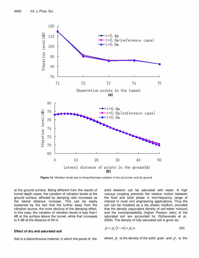
Effect of tunnel lining thickness

The tunnel lining thickness is considered with three

4398 Int. J. Phys. Sci.

(a)

(b) Figure 12. Vibration levels due to maglev train speed variation in the (a) tunnel, and (b) ground.

thicknesses: 0.4, 0.6 (reference case) and 0.8 m. Figure 14 shows the influences of the lining thickness to the vibration. As can be seen, the effect of lining thickness of tunnel on the vibration both in the tunnel and ground surface is negligible. As the stiffness of the tunnel is a very small proportion of overall stiffness of the tunnel-soil system, the stiffness of the tunnel-soil system is little affected by the lining thickness variation.

Effect of soil stiffness In order to investigate the effect of soil material stiffness on the results, a 50% variation in the elastic modulus of all soil layers of the reference model is imposed to make the soil softer and stiffer. The vibration levels affected by the soil stiffness are shown in Figure 15. The vibration level of the ground surface is sensitive to a deviation of

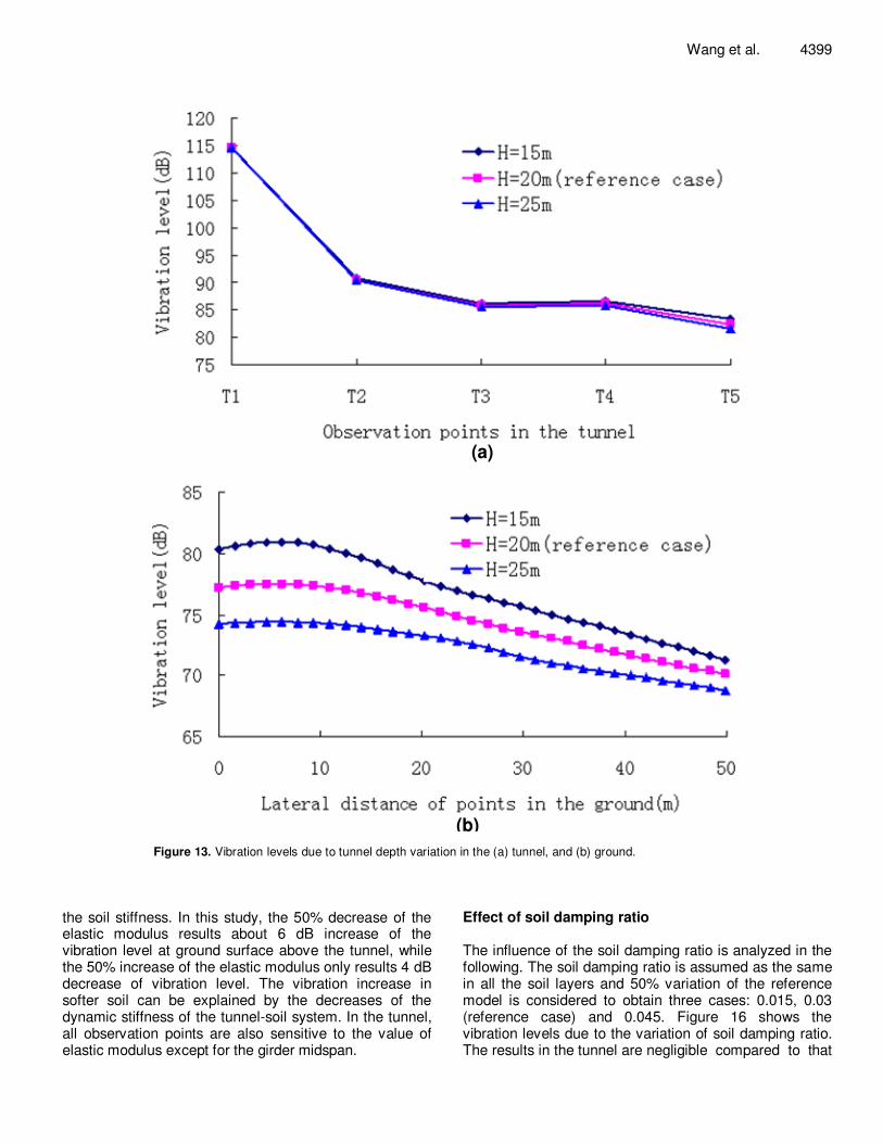
Wang et al. 4399

(a)

(b) Figure 13. Vibration levels due to tunnel depth variation in the (a) tunnel, and (b) ground.

the soil stiffness. In this study, the 50% decrease of the elastic modulus results about 6 dB increase of the vibration level at ground surface above the tunnel, while the 50% increase of the elastic modulus only results 4 dB decrease of vibration level. The vibration increase in softer soil can be explained by the decreases of the dynamic stiffness of the tunnel-soil system. In the tunnel, all observation points are also sensitive to the value of elastic modulus except for the girder midspan.

Effect of soil damping ratio The influence of the soil damping ratio is analyzed in the following. The soil damping ratio is assumed as the same in all the soil layers and 50% variation of the reference model is considered to obtain three cases: 0.015, 0.03 (reference case) and 0.045. Figure 16 shows the vibration levels due to the variation of soil damping ratio. The results in the tunnel are negligible compared to that

4400 Int. J. Phys. Sci.

(a)

(b) Figure 14. Vibration levels due to lining thickness variation in the (a) tunnel, and (b) ground.

at the ground surface. Being different from the results of tunnel depth cases, the variation of vibration levels at the ground surface, affected by damping ratio increases as the lateral distance increase. This can be easily explained by the fact that the further away from the vibration source, the more obvious of the damping effect. In this case, the variation of vibration levels is less than1 dB at the surface above the tunnel, while that increases to 5 dB at the distance of 50 m. Effect of dry and saturated soil Soil is a discontinuous material, in which the pores of the

solid skeleton can be saturated with water. A high viscous coupling prevents the relative motion between the fluid and solid phase in low-frequency range of interest in most civil engineering applications. Thus the soil can be modeled as a dry elastic medium, provided that the density (equivalent density of soil-water mixture) and the incompressibility (higher Poisson ratio) of the saturated soil are accounted for (Schevenels et al., 2004). The density of fully saturated soil is given as:

( )1s fn nρ ρ ρ= − + (24)

where s

ρ is the density of the solid grain and f

ρ is the

Wang et al. 4401

(a)

(b)

Figure 15. Vibration levels due to soil stiffness variation in the (a) tunnel, and (b) ground.

density of the pore fluid and n is the porosity. The

longitudinal wave velocity p

c and shear wave velocity s

c

of saturated soil in the low-frequency limit can be described as:

( )p s s f

s s

c K n

c

λ µ ρ

µ ρ

= + +

= (25)

Where s

λ and s

µ are the Lame´ coefficients of the dry

soil, f

K is the bulk modulus of the pore fluid and equals

to 2.2E+09 N/m2. The elastic modulus and Poisson ratio

of saturated soil can be computed by p

c and s

c .Here, a

dry soil (reference case) and a fully saturated soil case are investigated. The porosity of the fully saturated soil is considered as 0.3 for all soil layers. The effects of the two cases on the vibration levels are shown in Figure 17. The fully saturated soil has a larger vibration reduction than the dry soil both in the tunnel and ground surface except for the girder midspan, which is similar to the effect of the larger soil elastic modulus. This is due to that the dry soil has a higher incompressibility comparing to saturated soil. The value reduction in decibel is about 3 dB at the ground surface in this case.

4402 Int. J. Phys. Sci.

(a)

(b) Figure 16. Vibration levels due to soil damping ratio variation in the (a) tunnel, and (b) ground.

Conclusions In this paper, a 3D maglev train-guideway-tunnel-soil model is presented to study the dynamic response due to the high speed EMS maglev vehicle travelling in a tunnel. The maglev train is modeled by multi-rigid bodies, and the guideway, tunnel and soil are modeled by finite elements with PML artificial boundary. The interaction between the maglev train and guideway is modeled by

linear spring-damping system, which is accurate enough for the simulation of magnetic force considering the 10 mm airgap and its small variance in the high speed EMS maglev system. Comparing with the German design guideline, the numerical results of the dynamic factor at the girder midspan show small differences at low velocity but appear conservative at higher velocity of more than 200 km/h. In order to investigate the maglev train, tunnel and soil parameters on the dynamic response of tunnel

Wang et al. 4403

(a)

(b)

Figure 17. Vibration levels of dry and saturated soil in the (a) tunnel (b) ground.

and ground surface, the summation of velocity level for the 1/3 octave band is used to quantify the vibration induced by underground high speed maglev train. Some conclusions are drawn from the parametric studies as follows:

The vibration attenuates little when it is transferred from the girder support to the tunnel because of the rigid connection. Elastic rubber pad could be added between the girder support and the tunnel floor for further vibration attenuation. An increase in the maglev train speed is accompanied by an increase in the vibration levels in the tunnel and ground surface, and a difference of about 3 to

5 dB in vibration levels at small lateral distances from the tunnel is observed due to a 50 km/h variation in the maglev train speed. The vibration levels in the tunnel are little affected by the variation of the tunnel depth, but that at the ground surface decrease with the tunnel depth. The variation of the vibration level at the ground surface gradually decreases as the lateral distance increases. The effect of tunnel lining thickness on the vibration levels in the tunnel and ground surface is insignificant. The variation of the soil elastic modulus reveals that the vibration levels in the tunnel and ground surface are sensitive to the soil stiffness. Softer soil results higher

4404 Int. J. Phys. Sci. vibration levels due to the decrease of dynamic stiffness of the tunnel-soil system. The influence of the soil damping ratio on the vibration in the tunnel is negligible compared to that at the ground surface, and the differences of vibration levels due to damping ratio variation at the ground surface shows a trend of increasing with the increase of the lateral distance. The saturated soil has a larger vibration reduction than the dry soil both in the tunnel and ground surface, which shows a similar effect by the softer soil. ACKNOWLEDGEMENTS This work is supported by National Natural Science Foundation of China (No.50875166, 11072150 and 61073088), Research Project of State Key Laboratory of Mechanical System and Vibration (No. MSVMS201107), Scientific and Technological Research Project of Shanghai Science and Technology Committee (No.09231203100). REFERENCES Andersen L, Jones CJC (2006). Coupled boundary and finite element

analysis of vibration from railway tunnels-A comparison of two- and three-dimensional models. J. Sound Vib., 293(3-5):611-625.

Basu U (2009). Explicit finite element perfectly matched layer for transient three-dimensional elastic waves. Int. J. Numer. Meth. Eng., 77(2): 151-176.

Basu U, Chopra AK (2003). Perfectly matched layers for time-harmonic elastodynamics of unbounded domains: theory and finite-element implementation. Comput. Meth. Appl. Mech. Eng., 192(11-12):1337-1375.

Basu U, Chopra AK (2004). Perfectly matched layers for transient elastodynamics of unbounded domains. Int. J. Numer. Meth. Eng., 59(8): 1039-1074.

Benson DJ, Hallquist JO (1986). A simple rigid body algorithm for structural dynamics program. Int. J. Numer. Methods Eng., 22(3):723-749.

Bindel DS, Govindjee S (2005). Elastic PMLs for resonator anchor loss simulation. Int. J. Numer. Meth. Eng., 64(6):789-818.

Gardien W, Stuit HG (2003). Modelling of soil vibrations from railway tunnels. J. Sound Vib., 267(3):605-619.

Gupta S, Stanus Y, Lombaert G, Degrande G (2009). Influence of tunnel and soil parameters on vibrations from underground railways. J. Sound Vib., 327(1-2):70-91.

Hughes TJR, Winget J (1980). Finite rotation effects in numerical integration of rate constitutive equations arising in large-deformation analyses. Int. J. Numer. Meth. Eng., 15(12):1862-1867.

International Organization for Standardization (2005). ISO 14837-1:2005 Mechanical vibration-ground-borne noise and vibration arising from rail systems-part 1: general guidance.

Ju SH (2007). Finite element analysis of structure-borne vibration from high-speed train. Soil Dyn. Earthqu. Eng., 27(3):259-273.

Lee HW, Kim KC, Lee J (2006). Review of maglev train technologies.

IEEE Trans. Magn., 42(7):1917-1925. Lee JS, Kwon SD, Kim MY, Yeo IH (2009). A parametric study on the

dynamics of urban transit maglev vehicle running on flexible guideway bridges. J. Sound Vib., 328(3):301-317.

Magnetschnellbahn Ausführungsgrundlage Fahrweg (2007). Teil II, Eisenbahn-Bundesamt. Bonn, Germany.

Ma S, Liu P (2006). Modeling of the perfectly matched layer absorbing boundaries and intrinsic attenuation in explicit finite-element methods. Bull. Seismol. Soc. Am., 96(5):1779-1794.

Hägele N, Dignath F (2009). Vertical dynamics of the Maglev vehicle Transrapid. Multibody Syst. Dyn., 21(3):213-231.

Schevenels M, Degrande G, Lombaert G (2004). The influence of the depth of the ground water table on free field road traffic induced vibrations. Int. J. Numer. Anal. Methods Geomech., 28(5): 395-419.

Sheng X, Jones CJC, Thompson DJ (2006). Prediction of ground vibration from trains using the wavenumber finite and boundary element methods. J. Sound Vib., 293(3-5):575-586.

Shi J, Wei QC, Zhao Y (2007). Analysis of dynamic response of the high-speed EMS maglev vehicle/guideway coupling system with random irregularity. Veh. Syst. Dyn., 45(12):1077-1095.

Yang YB, ASCE F, Hung HH (2008). Soil vibrations caused by underground moving trains. J. Geotech. Geoenviron. Eng., 134(11):1633-1644.

Zhao CF, Zhai WM (2002). Maglev vehicle/guideway vertical random response and ride quality. Veh. Syst. Dyn., 38(3):185-209.

Zhai W, Song E (2010). Three dimensional FEM of moving coordinates for the analysis of transient vibrations due to moving loads. Comput. Geotech., 37(1-2):164-174.