Modeling and Recognition of Landmark Image Collections Using

Noname manuscript No.(will be inserted by the editor)

Modeling and Recognition of Landmark Image CollectionsUsing Iconic Scene Graphs

Rahul Raguram · Changchang Wu · Jan-Michael Frahm · SvetlanaLazebnik

Received: date / Accepted: date

Abstract This article presents an approach for mod-eling landmarks based on large-scale, heavily contami-nated image collections gathered from the Internet. Oursystem efficiently combines 2D appearance and 3D geo-metric constraints to extract scene summaries and con-struct 3D models. In the first stage of processing, im-ages are clustered based on low-dimensional global ap-pearance descriptors, and the clusters are refined using3D geometric constraints. Each valid cluster is repre-sented by a single iconic view, and the geometric re-lationships between iconic views are captured by aniconic scene graph. Using structure from motion tech-niques, the system then registers the iconic images toefficiently produce 3D models of the different aspects ofthe landmark. To improve coverage of the scene, these3D models are subsequently extended using additional,non-iconic views. We also demonstrate the use of iconicimages for recognition and browsing. Our experimentalresults demonstrate the ability to process datasets con-taining up to 46,000 images in less than 20 hours, usinga single commodity PC equipped with a graphics card.This is a significant advance towards Internet-scale op-eration.

1 Introduction

Today, more than ever before, it is evident that “to col-lect photography is to collect the world” [Sontag, 1977].More and more of the Earth’s cities and sights are pho-tographed each day from a variety of digital cameras,viewing positions and angles, weather and illuminationconditions; more and more of these photos get tagged

Dept. of Computer Science, University of North Carolina, ChapelHill, NC 27599-3175E-mail: {rraguram,ccwu,jmf,lazebnik}@cs.unc.edu

by users and uploaded to photo-sharing websites. Forexample, on Flickr.com, locations form the single mostpopular category of user-supplied tags [Sigurbjornssonand van Zwol, 2008]. With the growth of community-contributed collections of place-specific imagery, therecomes a growing need for algorithms that can distilltheir content into representations suitable for summa-rization, visualization, and browsing.

In this article, we consider collections of Flickr im-ages associated with a landmark keyword such as “Statueof Liberty,” with often noisy annotations and metadata.Our goal is to efficiently identify all photos that actu-ally represent the landmark of interest, and to organizethese photos to reveal the spatial and semantic struc-ture of the landmark. Any system that aims to meetthis goal must address several challenges inherent inthe nature of the data:– Contamination: When dealing with community-

contributed landmark photo collections, it has beenobserved that keywords and tags are accurate onlyapproximately 50% of the time [Kennedy et al., 2006].Since we obtain our input using keyword searches,a large fraction of the input images comprises of“noise,” or images that are unrelated to the conceptof interest.

– Diversity: The issue of contamination aside, even“valid” depictions of landmarks have a remarkabledegree of diversity. Landmarks may have multipleaspects (sometimes geographically dispersed), theymay be photographed at different times of day andin different weather conditions, to say nothing ofnon-photorealistic depictions and cultural references(Figure 1).

– Scale: The typical collection of photos annotatedwith a landmark-specific phrase has tens to hun-dreds of thousands of images. For example, there

2

Fig. 1 The diversity of photographs depicting “Statue of Lib-erty.” There are copies of the statue in New York, Las Vegas,Tokyo, and Paris. The appearance of the images can vary signif-icantly based on time of day and weather conditions. Furthercomplicating the picture are parodies (e.g., people dressed asthe statue) and non-photorealistic representations. The approachpresented in this article relies on rigid 3D constraints, so it is notapplicable to the latter two types of depictions.

are over 140,000 images on Flickr associated withthe keyword “Statue of Liberty.” If we wanted toprocess such collections using a traditional structurefrom motion (SfM) pipeline, we would have to takeevery pair of images and try to establish a two-viewrelation between them. The running time of such anapproach would be at least quadratic in the numberof input images. Clearly, such brute-force matchingis not scalable; we need smarter and more efficientways of organizing the images.

Fortunately, landmark photo collections also possesshelpful characteristics that can actually make large-scale modeling easier. The main such characteristic isredundancy: people tend to take pictures from certainviewpoints and to frame their compositions in consis-tent ways, giving rise to many large groups of verysimilar-looking photos. Our system is based on the ob-servation that such groups can be discovered using 2Dappearance-based constraints that are considerably moreefficient than full-blown SfM constraints, and that theiconic views representing these groups form a completeand concise summary of the scene, so that most of thesubsequent computation can be restricted to the iconicviews without much loss of content.

Figure 2 gives an overview of our system and Algo-rithm 1 shows a more detailed summary of the mod-eling steps. Our system begins by clustering all inputimages based on 2D appearance descriptors, and then itprogressively refines these clusters with geometric con-straints to select iconic images that represent dominantaspects of the scene. These images and the pairwisegeometric relationships between them define an iconic

scene graph. In the next step, this graph is used forefficient reconstruction of a 3D skeleton model, whichis subsequently extended using additional relevant im-ages. Given a new test image, we can register it intothe model in order to answer the question of whetherthe landmark is present in the test image. In addition,as a natural consequence of the structure of our ap-proach, the image collection can be cleanly organizedinto a hierarchy for browsing.

Since our method efficiently filters out unrelated im-ages using 2D appearance-based constraints, which arecomputationally cheap, and applies more computation-ally demanding geometric constraints to much smallersubsets of “promising” images, it is scalable to largephoto collections. Unlike approaches based purely onSfM, e.g., [Agarwal et al., 2009], it does not requirea massively parallel cluster of hundreds of computingcores and can process datasets consisting of tens ofthousands of images within hours on a single commod-ity PC.

The rest of this article is organized as follows. Sec-tion 2 places our research in the context of other relatedwork on landmark modeling. In Section 3 we introducethe steps of our implemented system. Section 4 presentsexperimental results on three datasets: the Notre Damecathedral in Paris, Statue of Liberty, and Piazza SanMarco in Venice. Finally, Section 5 closes the presenta-tion with a discussion of limitations and directions forfuture work.

An earlier version of this work was originally pre-sented in [Li et al., 2008]. For the present article, thesystem has been completely re-implemented to includemuch faster GPU-based feature extraction and geomet-ric verification, an improved image registration algo-rithm leading to higher precision and recall, and a newincremental reconstruction strategy delivering larger andmore complete models. Videos of computed 3D models,along with complete browsing summaries, can be foundon the project website.1

2 Previous Work

Our system offers a comprehensive solution to the prob-lems of dataset collection, 3D reconstruction, scene sum-marization, browsing and recognition for landmark im-ages. In this section, we discuss related recent work inthese areas.

At a high level, one of the goals of our work canbe described as follows: starting with the heavily con-taminated output of an Internet image search query,we want to extract a high-precision subset of images

1 http://www.cs.unc.edu/PhotoCollectionReconstruction

3

Raw photo collection Iconic summary Iconic scene graph

R t ti

Query: “Statue of Liberty”47,238 images, ~40% irrelevant

454 images

Reconstruction

Hierarchical browsing

Las Vegas

New York

Tokyo

Fig. 2 Overview of our system. The input to the system is a raw, contaminated photo collection, which is reduced to a collectionof representative iconic images by 2D appearance-based clustering followed by geometric verification. The geometric relationshipsbetween iconic views are captured by the iconic scene graph. The structure of the iconic scene graph is used to automatically generate3D point cloud models, as well as to impose a hierarchical organization on the images for browsing. Videos of the models, along witha browsing interface, can be found at www.cs.unc.edu/PhotoCollectionReconstruction.

that are actually relevant to the query. Several exist-ing approaches consider this problem of dataset collec-tion for generic visual categories not characterized byrigid 3D structure[Fergus et al., 2004, Berg and Forsyth,2006, Li et al., 2007, Schroff et al., 2007, Collins et al.,2008]. These approaches use statistical models to com-bine different kinds of 2D image features (texture, color,keypoints), as well as text and tags. However, for ourspecific application of landmark modeling, such statis-tical models do not provide strong enough geometricconstraints. Philbin and Zisserman [2008], Zheng et al.[2009] have presented dataset collection and object dis-covery methods specifically adapted to landmarks. Thesemethods use indexing based on keypoints followed byloose geometric verification using 2D affine transfor-mations or spatial coherence filters. Unlike them, ourmethod includes an initial stage in which images areclustered using global image features, giving us a bigger

gain in efficiency and an improved ability to group simi-lar viewpoints. Another difference between our methodand [Philbin and Zisserman, 2008, Zheng et al., 2009]is that we perform geometric verification by applyingfull 3D SfM constraints instead of loose 2D spatial con-straints.

To discover all the images belonging to the land-mark, we first try to find a set of iconic views, corre-sponding to especially popular and salient aspects. Re-cently, a number of papers have proposed a very gen-eral notion of canonical or iconic images as good rep-resentative images for arbitrary visual categories [Bergand Berg, 2009, Jing and Baluja, 2008, Raguram andLazebnik, 2008]. These approaches try to find iconic im-ages essentially by 2D image clustering, with some pos-sible help from additional features such as text. Bergand Forsyth [2007], Kennedy and Naaman [2008] haveused similar 2D cues to select representative views of

4

landmarks without taking into account the full 3D con-straints associated with landmark scenes.

For rigid 3D object instances, canonical view selec-tion has been studied both in psychology [Palmer et al.,1981, Blanz et al., 1999] and in computer vision [Den-ton et al., 2004, Hall and Owen, 2005, Weinshall et al.,1994]. Palmer et al. [1981] propose several criteria todetermine whether a view is “canonical”, one of whichis particularly interesting for large image collections:When taking a photo, which view do you choose? Asobserved by Simon et al. [2007], community photo col-lections provide a likelihood distribution over the view-points from which people prefer to take photographs. Inthis context, canonical view selection can be thoughtof as identifying prominent clusters or modes of thisdistribution. Simon et al. [2007] find these modes byclustering images based on the output of local featurematching and epipolar geometry verification betweenevery pair of images in the dataset – steps that arenecessary for producing a full 3D reconstruction. Whilethis solution is effective, it is computationally expen-sive, and it treats scene summarization as a by-productof 3D reconstruction. By contrast, we regard summa-rization as an image organization step that precedesand facilitates 3D reconstruction.

The first approach for organizing unordered imagecollections was proposed by Schaffalitzky and Zisser-man [2002]. Sparse 3D reconstruction of landmarks fromInternet photo collections was first addressed by thePhoto Tourism system [Snavely et al., 2006, 2008b],which achieves high-quality reconstruction results withthe help of exhaustive pairwise image matching andglobal bundle adjustment of the model after insert-ing each new view. Unfortunately, this process doesnot scale to large datasets, and it is particularly in-efficient for heavily contaminated collections, most ofwhose images cannot be registered to each other. ThePhoto Tourism framework is more suited to the casewhere a user submits a predominantly “clean” set ofphotographs for 3D reconstruction and visualization.This is precisely the mode of input adopted by the Mi-crosoft Photosynth software,2 which is based on PhotoTourism.

After the appearance of Photo Tourism, several re-searchers have developed more efficient SfM methodsthat exploit the redundancy in community photo collec-tions. In particular, many landmark image collectionsconsist of a small number of “hot spots” from whichphotos are often taken. Ni et al. [2007] have proposeda technique for out-of-core bundle adjustment that lo-cally optimizes the “hot spots” and then connects thelocal solutions into a global one. In this paper, we fol-

2 http://photosynth.net

low a similar strategy of computing separate 3D recon-structions on connected sub-components of the scene,thus avoiding the need for frequent large-scale bundleadjustment. Snavely et al. [2008a] find skeletal sets ofimages from the collection whose reconstruction pro-vides a good approximation to a reconstruction involv-ing all the images. However, computing the skeletal setstill requires as an initial step the exhaustive verifica-tion of all two-view relationships in the dataset. Simi-larly to Snavely et al. [2008a], we find a small subset ofthe collection that captures all the important scene as-pects. But unlike Snavely et al. [2008a], we do not needto compute all the pairwise image relationships in thedataset; instead, we rely on 2D appearance similarityas a rough approximation of the “true” multi-view re-lationship, and reduce the number of possible pairwiserelationships to consider through an initial clusteringstage. As a result, our technique is capable of handlingdatasets that are an order of magnitude larger thanthose in [Snavely et al., 2008a], at a fraction of the run-ning time.

In another related recent work, Agarwal et al. [2009]present a distributed system for reconstructing verylarge-scale image collections. This system uses the corealgorithms from [Snavely et al., 2008b,a], implementedand optimized to harness the massive parallelism ofmulti-core clusters. To speed up the detection of ge-ometrically related images, Agarwal et al. [2009] usefeature-based indexing in conjunction with approximatenearest neighbor search [Arya et al., 1998]. They alsouse query expansion [Chum et al., 2007] to extend theinitial set of pairwise relationships. Using a computecluster with up to 500 cores, the system of Agarwalet al. [2009] is capable of reconstructing city-scale im-age collections containing 150,000 images in the spanof a day. These collections are larger than ours, but thecloud computing solution is expensive: it costs around$10,000 to rent a cluster of 1000 nodes for a day.3

By contrast, our system runs on a single commodityPC and uses a combination of efficient algorithms andlow-cost graphics hardware to achieve fast performance.Specifically, our system currently processes up to 46,000images in approximately 20 hours using a PC with anIntel core2 duo processor with 3GHz and 2.5GB RAMas well as an NVidia GTX 280 graphics card.

Finally, unlike [Agarwal et al., 2009, Ni et al., 2007,Snavely et al., 2008a,b], our approach is concerned notonly with reconstruction, but also with recognition. Wepose landmark recognition as a binary problem – givena query image, find out whether it contains an instanceof the landmark of interest – and solve it by attempt-ing to retrieve iconic images similar to the test query.

3 http://aws.amazon.com/ec2

5

Algorithm 1 System Overview1. Initial clustering (Section 3.1): Run k-means clusteringon global gist descriptors to partition the image collection intoclusters corresponding to approximately similar viewpoints andscene conditions.2. Geometric verification and iconic image selection(Section 3.2): Perform robust pairwise epipolar geometry es-timation between a few top images in each cluster. Reject allclusters that do not have enough geometrically consistent im-ages. For each remaining cluster, select an iconic image as theimage that gathers the most inliers to the other top images,and discard all cluster images inconsistent with the iconic.3. Re-clustering and registration (Section 3.3): Performclustering and geometric verification on the images discardedduring Step 2. This enables the discovery of smaller iconic clus-ters. After identifying additional iconic images, make a finalpass over the discarded images and attempt to register themto any of the iconics.4. Computing the iconic scene graph (Section 3.4): Regis-ter each pair of iconic images to each other and create a graphwhose nodes correspond to iconic images, edges correspondto valid two-view transformations between iconics, and edgeweights are given by the number of feature inliers to the re-spective transformations. This graph will be used to guide thesubsequent 3D reconstruction process. Use tag information toreject isolated nodes of the iconic scene graph that are likelyto be semantically unrelated to the landmark.5. 3D reconstruction (Section 3.5): Efficiently reconstructsparse 3D models from the set of images registered to the iconicrepresentation. The reconstruction proceeds in an incremen-tal fashion, by first building multiple 3D sub-models from theiconics, merging them whenever possible, and finally growingall models by incorporating additional non-iconic images.

To accomplish this task, we use methods common toother state-of-the-art retrieval techniques, including in-dexing based on local image features and geometric ver-ification [Chum et al., 2007, Philbin et al., 2008]. Ofcourse, alternative formulations of the landmark recog-nition problem are also possible. For example, Li et al.[2009] perform multi-class landmark recognition usinga more statistical approach based on a support vectormachine classifier. At present, we have not incorporateda discriminative statistical model into our recognitionapproach. However, we expect that classifiers trainedon automatically extracted sets of iconic images corre-sponding to many different landmarks would producevery satisfactory results.

3 The Approach

In this section, we present a description of the compo-nents of our landmark modeling system. Algorithm 1gives a high-level summary of these components, andFigure 2 illustrates the operation of the system.

3.1 Initial Clustering

The first step of our system is to identify a small setof iconic views to summarize the scene content. Simi-larly to Simon et al. [2007], we define iconic views asrepresentatives of dense clusters of similar viewpoints.However, while Simon et al. [2007] define similarity ofany two views in terms of the number of 3D featuresthey have in common, we adopt a more perceptual cri-terion. Namely, if there are many images in the datasetthat share a very similar viewpoint in 3D, then a num-ber of them will have a very similar image appearancein 2D, and they can be grouped efficiently using a low-dimensional global description of their pixel patterns.

The global descriptor we use is gist [Oliva and Tor-ralba, 2001], which was found to be effective for group-ing images by perceptual similarity and retrieving struc-turally similar scenes [Hays and Efros, 2007, Douzeet al., 2009]. We generate a gist descriptor for eachimage in the dataset by computing oriented edge re-sponses at three scales (with 8, 8 and 4 orientations,respectively), aggregated to a 4 × 4 spatial resolution.In addition, we augment this gist descriptor with colorinformation, consisting of a subsampled image, at 4×4spatial resolution. We thus obtain a 368-dimensionalvector as a representation of each image in the dataset.We implemented gist extraction as a series of convolu-tions on the GPU4, achieving computation rates of 170Hz (see Table 2 for detailed timings).

In order to identify typical views, we cluster the gistdescriptors of all our input images using the k-meansalgorithm. In this initial stage, it is acceptable to pro-duce an over-clustering of the scene, since in subsequentstages, we will be able to restore links between clustersthat have sufficient viewpoint similarity. For this rea-son, we set the number of clusters k to be fairly high(k = 1200 in the experiments, although the outcome isnot very dependent on the exact value used). In all ofour experiments, the resulting clusters capture the pop-ular viewpoints quite well. In particular, the largest gistclusters tend to be quite clean (Figure 3). If we rank thegist clusters in decreasing order of size, we can see thatthe top few clusters have a remarkably high precision(Figure 7, Stage 1 curve).

3.2 Geometric Verification and Iconic Image Selection

Of course, clustering based on low-dimensional globaldescriptors has its drawbacks. For one, the gist descrip-tor is sensitive to image variation such as clutter (for

4 code in preparation for release

6

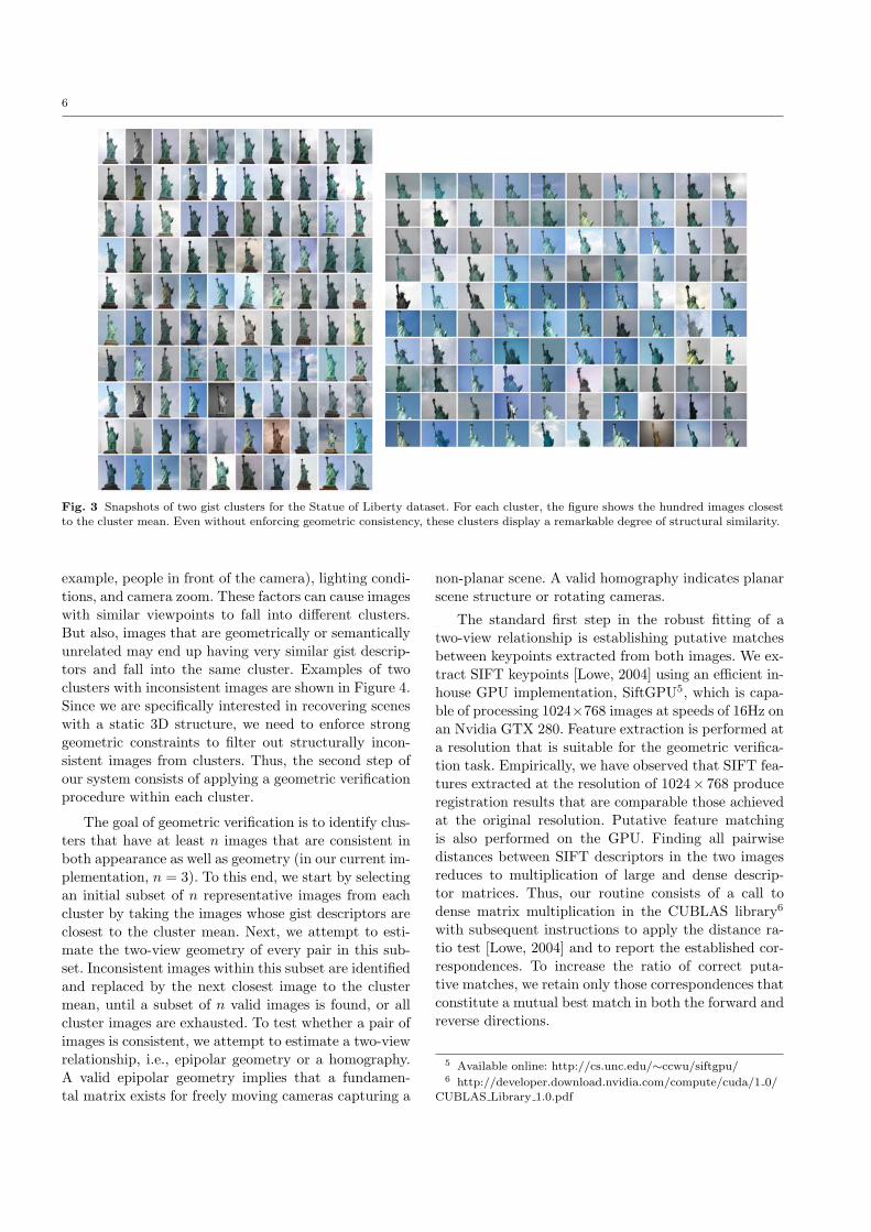
Fig. 3 Snapshots of two gist clusters for the Statue of Liberty dataset. For each cluster, the figure shows the hundred images closestto the cluster mean. Even without enforcing geometric consistency, these clusters display a remarkable degree of structural similarity.

example, people in front of the camera), lighting condi-tions, and camera zoom. These factors can cause imageswith similar viewpoints to fall into different clusters.But also, images that are geometrically or semanticallyunrelated may end up having very similar gist descrip-tors and fall into the same cluster. Examples of twoclusters with inconsistent images are shown in Figure 4.Since we are specifically interested in recovering sceneswith a static 3D structure, we need to enforce stronggeometric constraints to filter out structurally incon-sistent images from clusters. Thus, the second step ofour system consists of applying a geometric verificationprocedure within each cluster.

The goal of geometric verification is to identify clus-ters that have at least n images that are consistent inboth appearance as well as geometry (in our current im-plementation, n = 3). To this end, we start by selectingan initial subset of n representative images from eachcluster by taking the images whose gist descriptors areclosest to the cluster mean. Next, we attempt to esti-mate the two-view geometry of every pair in this sub-set. Inconsistent images within this subset are identifiedand replaced by the next closest image to the clustermean, until a subset of n valid images is found, or allcluster images are exhausted. To test whether a pair ofimages is consistent, we attempt to estimate a two-viewrelationship, i.e., epipolar geometry or a homography.A valid epipolar geometry implies that a fundamen-tal matrix exists for freely moving cameras capturing a

non-planar scene. A valid homography indicates planarscene structure or rotating cameras.

The standard first step in the robust fitting of atwo-view relationship is establishing putative matchesbetween keypoints extracted from both images. We ex-tract SIFT keypoints [Lowe, 2004] using an efficient in-house GPU implementation, SiftGPU5, which is capa-ble of processing 1024×768 images at speeds of 16Hz onan Nvidia GTX 280. Feature extraction is performed ata resolution that is suitable for the geometric verifica-tion task. Empirically, we have observed that SIFT fea-tures extracted at the resolution of 1024× 768 produceregistration results that are comparable those achievedat the original resolution. Putative feature matchingis also performed on the GPU. Finding all pairwisedistances between SIFT descriptors in the two imagesreduces to multiplication of large and dense descrip-tor matrices. Thus, our routine consists of a call todense matrix multiplication in the CUBLAS library6

with subsequent instructions to apply the distance ra-tio test [Lowe, 2004] and to report the established cor-respondences. To increase the ratio of correct puta-tive matches, we retain only those correspondences thatconstitute a mutual best match in both the forward andreverse directions.

5 Available online: http://cs.unc.edu/∼ccwu/siftgpu/6 http://developer.download.nvidia.com/compute/cuda/1 0/

CUBLAS Library 1.0.pdf

7

Fig. 4 Snapshots of two clusters containing images inconsistent with the dominant 3D structure. By enforcing two-view geometricconstraints, these images (outlined in red) are filtered out.

Once putative matches have been established, weestimate the two-view relationship between the imagesby applying ARRSAC [Raguram et al., 2008], whichis a robust estimation framework capable of real-timeperformance. We couple this estimation algorithm withQDEGSAC [Frahm and Pollefeys, 2006], which is a ro-bust model selection procedure that accounts for dif-ferent types of camera motion and scene degeneracies,returning either an estimate for a fundamental matrixor a homography depending on the scene structure andcamera motion. If the estimated relation is supportedby less than m inliers (m=18 in the implementation),the images are deemed inconsistent.

The image that gathers the largest total number ofinliers to the other n−1 representatives from its clusteris declared the iconic image of that cluster. The inlierscore of each iconic can be used as a measure of thequality of each cluster. Precision/recall curves in Fig-ure 7 (Stage 2a) demonstrate that inlier number of theiconic does a better job than cluster size in separatingthe “good” clusters from the “bad” ones. Note, how-ever, that ranking of clusters based on inlier numberof the iconic does not penalize clusters that have a fewgeometrically consistent images but are otherwise filledwith garbage. Once the iconic images for every clus-ter are selected, we perform geometric verification forevery remaining image by matching it to the iconic ofits cluster and rejecting it if it has fewer than m in-liers. As shown in Figure 7 (Stage 2b), this individualverification improves precision considerably.

As can be seen from Table 2 (Stage 2 column), ge-ometric verification takes just under an hour on theStatue of Liberty dataset, and just under half an houron the two other datasets. It is important to note thatefficiency gains in this step come not only from limit-ing the number of pairwise geometric verifications, butalso from targeting the verifications towards the right

image pairs. After all, robust estimation of two-viewgeometry tends to be fast for images that are geometri-cally related and therefore have a high inlier ratio, whilefor unrelated images, the absence of a geometric rela-tion can only be determined by carrying out the max-imum number of RANSAC iterations. Since images inthe same gist cluster are more likely to be geometricallyrelated, the average number of ARRSAC iterations forwithin-cluster verifications is comparably low.

3.3 Re-clustering and Registration

While the geometric verification stage raises the preci-sion of the registered images, it also lowers the overallrecall by rejecting relevant images that didn’t happento be geometrically consistent with the chosen iconic oftheir clusters. Such images often come from less com-mon aspects of the landmark that did not manage to gettheir own cluster initially. To recover such aspects, wepool together all images that were discarded in the pre-vious step, and apply a second round of clustering andverification. As in Section 3.2, we select a single iconicrepresentative per each new valid cluster. As shown inTable 2, this contributes a substantial number of addi-tional iconics to the representation.

After augmenting the initial set of iconics, we per-form a final “cleanup” attempting to match each left-over image to the discovered scene structure. In order toefficiently do this, we retrieve, for each leftover image,the k nearest iconics in terms of gist descriptor distance(with k=10 in our current implementation), attempt toregister the image to each of those iconics, and assign itto the cluster of the iconic with which it gets the mostinliers (provided, of course, that the number of inliersexceeds our minimum threshold).

8

As seen in Figure 7 (Stage 3), re-clustering and reg-istration increases recall of relevant images from 33%to 50% on the Statue of Liberty, from 46% to 66% onthe San Marco dataset, and from 38% to 60% on NotreDame. In terms of computation time, re-clustering andregistration takes about three times as long as the ini-tial geometric verification (Table 2, Stage 3 column).The bulk of this time is spent attempting to registerall leftover images to all iconics, since, not surprisingly,the inlier ratios of such images tend to be relativelylow. Even with the additional computational expense,the overall geometric verification portion of our algo-rithm compares quite favorably to that of the fastestsystem to date [Agarwal et al., 2009], which uses mas-sive parallelism and feature-based indexing to speed upputative matching. On the Statue of Liberty dataset,our system performs both stages of clustering and veri-fication on about 46,000 images in approximately sevenhours on one core (Table 2, Totals column). For theanalogous processing stages, Agarwal et al. [2009] re-port a running time of five hours on 352 cores (in otherwords, 250 times more core hours than our system) fora dataset of only 1.3 times the size.

3.4 Constructing the Iconic Scene Graph

The next step of our system is to build an iconic scenegraph to capture the full geometric relationships be-tween the iconic views and to guide the subsequent3D reconstruction process. To do this, we perform fea-ture matching and geometric verification between eachpair of iconic images. Note that in our experiments, thenumber of iconics is orders of magnitude smaller thanthe total dataset size (several hundred iconics vs. tens ofthousands initial images), so exhaustive pairwise verifi-cation of iconics is fast. Feature matching is carried outusing the techniques described in Section 3.2, but thegeometric verification procedure is different. For verify-ing the geometric consistency of clusters, we sought toestimate a fundamental matrix or a homography. Butnow, as a prelude to the upcoming SfM stage, we seekto obtain a two-view metric reconstruction.

Pairwise metric 3D reconstructions can be obtainedby the five-point relative pose estimation algorithm [Nister,2004] and triangulating 3D points based on 2D featurematches. This algorithm requires estimates of internalcalibration parameters for each of the cameras. To getthese estimates, we make the zero skew assumption andinitialize the principal point to be in the center of eachimage; for the focal length, we either read the EXIFdata or use the camera specs for a common viewing an-gle. In practice, this initialization tends to be within the

calibration error threshold of 10% tolerated by the five-point algorithm [Nister, 2004], and in the latter stagesof reconstruction, global bundle adjustment refines thecalibration parameters.7 Note that the inlier ratios ofputative matches between pairs of iconic images tend tobe very high and consequently, the five-point algorithmrequires very few RANSAC iterations. For instance, inthe Statue of Liberty dataset, of the image pairs thatcontain at least 20 putative matches, 80% of the pairshave an inlier ratio larger than 50%.

After estimating the two-view pose for every pairof iconic images, we construct the iconic scene graph,where nodes are iconic images, and the weight of theedge connecting two iconics is defined to be the num-ber of inliers to their estimated pose. Iconic pairs withtoo few inliers (less than m) are given zero edge weightand are thus disconnected in the graph. For all of ourdatasets, the iconic scene graphs have multiple con-nected components corresponding to non-overlappingviewpoints, day vs. night views, or even geographicallyseparated instances of the landmark (e.g., copies of theStatue of Liberty in different cities).

In general, lacking GPS coordinates or higher-levelknowledge, we do not have enough information to deter-mine whether a given connected component is semanti-cally related to the landmark. However, we have noticedthat single-node connected components are very likelyto be semantically irrelevant. In many cases, they corre-spond to groups of near-duplicate images taken by a sin-gle user and incorrectly tagged (see Figure 5). To pruneout such clusters, we use a rudimentary but effective fil-ter based on image tags. First, we create a “referencelist” of tags that are considered to be semantically rele-vant to the landmark by taking the tags from all iconicimages that have at least two connections to other icon-ics (empirically, these are almost certain to contain thelandmark). To have a more complete list, we also incor-porate tags from the top ten cluster images registeredto these iconics. The tags in the list are ranked in de-creasing order of frequency. Next, isolated iconic imagesare scored based on the median rank of their tags in thereference list. Tags that do not occur in the list at allare assigned an arbitrary high number. Clusters witha high median rank are considered to be unrelated tothe landmark and removed from the dataset. As shownby the Stage 4 curves in Figure 7, this further improves

7 Note that our initial focal length estimate can be wrong forcameras with interchangeable lenses. The error can be particu-larly large for very long focal lengths, resulting in camera centerestimates that are displaced towards the scene points. For exam-ple, for a zoomed-in view of Statue of Liberty’s head, the esti-mated camera center may be pushed off the ground towards the

head. Some of this effect is visible in Figure 11.

9

Tags: italy liberty florence europe santacroce church firenze

Tags: letterman late show groundzero timesquare goodmorningamerica

Tags: newyorkcity fireworks victoria statueofliberty queenmary2 queenelizabeth2

Fig. 5 Sample clusters from the Statue of Liberty dataset that were discarded by tag filtering. Each of these clusters is internally

geometrically consistent, but does not have connections to any other clusters. By performing a simple tag-based filtering procedure,

these spurious iconics can be identified and discarded. Note that in downloading the images, we used Flickr’s full text search option,so that “Statue of Liberty” does not actually show up as a tag on every image in the dataset.

precision over the previous appearance- and geometry-based filtering stages.

3.5 Reconstruction

This section describes our novel incremental approachto reconstructing point cloud 3D models from the setof iconic images. The algorithm starts by building mul-tiple 3D sub-models covering the iconic scene graph,then it looks for common 3D features to merge differentsub-models, and finally, it grows the resulting modelsby registering into them as many additional non-iconicviews as possible. The sequence of these steps is shownin Algorithm 2 and discussed in detail below.

To initialize the process of incremental 3D recon-struction, we pick the pair of iconic images whose two-view reconstruction (computed as described in Section3.4) has the highest inlier number and delivers a suffi-ciently low reconstruction uncertainty, as computed bythe criterion of Beder and Steffen [2006]. Next, we it-eratively register additional cameras to this model. Ateach iteration, we propagate correspondences from thereconstructed 3D points to the iconics not yet in themodel that see these points. Then we take the iconicthat has the highest number of correct 2D-3D corre-spondences to the current sub-model, register it to thesub-model, and triangulate new 3D points from 2D-2Dmatches between the iconic and other images alreadyin the model. After each iteration, the 3D sub-modeland camera parameters are optimized by an in-houseimplementation of fast non-linear sparse bundle adjust-

ment8. If no further iconics have enough 2D-3D inliersto the current sub-model, the process starts afresh bypicking the next best pair of iconics not yet registeredto any sub-model. Thus, by iterating over the pool ofunregistered iconic images, multiple 3D sub-models arereconstructed.

The above process may produce multiple sub-modelsthat contain overlapping 3D structure and even sharesome of the same images, but that were not recon-structed together because neither one of the modelshas a single iconic with a sufficient number of 2D-3Dmatches to another model. Instead, such models may belinked by a larger number of images having relativelyfew correspondences each. To account for this case, ev-ery time we finish constructing a sub-model, we collectall 3D point matches between it and each of the mod-els already reconstructed, and merge it with a previousmodel provided a sufficient number of such matches ex-ist. The merging step uses ARRSAC to robustly esti-mate a similarity transformation based on the identified3D matches.

Even after the initial merging, we may end up withseveral separate sub-models coming from the same con-nected component of the iconic scene graph. This hap-pens when none of the connections between iconic im-ages in different sub-models are sufficient for direct reg-istration. To successfully merge such models, we need tosearch for additional non-iconic images to provide themissing links. To identify the most promising merginglocations, we consider pairs of source and target iconicsthat belong to two different models and are connected

8 Available online: http://cs.unc.edu/∼cmzach/oss/SSBA-

1.0.zip

10

Algorithm 2 Incremental ReconstructionExtract connected components of the iconic scene graph andtheir spanning trees.for each connected component do

[Incrementally build and merge sub-models.]

while suitable initial iconic pairs exist doCreate 3D sub-model from initial pair.while there exist unregistered iconic images with enough

2D-3D matches to sub-model doExtend the sub-model to the image with the most 2D-3D matches.Perform bundle adjustment to refine the sub-model.

end whileCheck for 3D matches between current sub-model andother sub-models in the same component and merge sub-models if there are sufficient 3D matches.

end while

[Attempt to discover non-iconic links between models.]

for each pair of sub-models connected in the spanning treedo

Search for additional non-iconic images to provide com-mon 3D points between the sub-models (see text).If enough enough common 3D points found, merge thesub-models.

end for

[Grow models by registering non-iconic images.]for each 3D model do

while there exist unregistered non-iconic images withenough 2D-3D matches to the model do

Expand model by adding non-iconic image with high-est number of 2D-3D correspondences.If more than 25 images added to model, perform bun-dle adjustment.

end whileend for

end for

by an edge of the maximal spanning tree (MST) of theiconic scene graph, and we search for non-iconic imagesthat can be registered to both of them. The search isconducted in the iconic clusters of the source and thetarget, as well as in the clusters of other iconics con-nected to the source in the MST (Figure 6). To maintainefficiency, we stop the search after finding five imageswith a sufficient number of correspondences both to thesource and the target. The triplet correspondences arethen registered into the 3D sub-models of the sourceand the target, providing common 3D points for merg-ing. We apply an analogous linking process to attemptto register iconic images that could not be placed inany 3D sub-model.

At this point, most of the models having commonstructure are typically merged together, and in theirtotality, the models cover most of the scene contentpresent in the iconic images. In the last stage of thereconstruction algorithm, we try to make the models

as complete as possible by incorporating non-iconic im-ages from clusters of the registered iconics. This processtakes advantage of feature matches between the non-iconic images and their respective iconics that were es-tablished during the earlier geometric verification stage(Section 3.2). The 2D matches between the image andits iconic determine 2D-3D correspondences betweenthe image and the 3D model into which the iconic isregistered, and ARRSAC is used to determine the cam-era pose. Since the model structure at this point tendsto be fairly stable, we carry out a full bundle adjust-ment after adding every 25 images. Detailed results ofour 3D reconstruction algorithm are shown in Figures11-16, and timings are presented in Table 3.

4 Experimental Results

We have tested our system on three large landmarkimage datasets: the Statue of Liberty (47,238 images),Piazza San Marco in Venice (45,322 images), and theNotre Dame cathedral in Paris (11,900 images). Eachof these datasets presents different challenges for oursystem: for example, the relative lack of texture onthe Statue of Liberty poses a problem for SIFT-basedmatching, while the often cluttered San Marco squareposes a challenge for gist clustering.

4.1 Data Collection

The datasets used for evaluation were automaticallydownloaded from Flickr.com using keyword searches.We randomly split each dataset into a “modeling” part,which forms the input to the system described in Sec-tion 3, and a much smaller independent “testing” part,which will be used to evaluate recognition performancein Section 4.4. Because the modeling datasets containtens of thousands of images, we have chosen to labelonly a small randomly selected fraction of them. Notethat the ground-truth labels are not used by the mod-eling algorithm itself; they are needed only to measurerecall and precision for the different stages described inSections 3.1-3.4. The smaller test sets are completelylabeled. Our labeling is very basic, merely recordingwhether the landmark is present in the image or not,without evaluating the quality or geometric fidelity ofa given view. In particular, artistic depictions of land-marks are labeled as positive, even though they can-not be registered to our iconic representation using SfMconstraints. Table 1 gives a breakdown of the numbersof labeled and unlabeled images in each of our datasets.The proportions of negative images (40% to 60%) givea good idea of the initial amount of contamination.

11

… …maximal�spanning�

treesub-model 1

…cluster of iconic connected to sourcecluster of iconic connected to source

…source source cluster

…target clustertarget target cluster

sub-model 2…

g

potential links between source and target

Fig. 6 3D sub-model merging: The target and source iconics are not registered in the same 3D sub-model due to a lack of common3D points. In this case, the source iconic is registered to a sub-model encompassing mainly the front of the San Marco square, andthe target is registered to a sub-model of the back of the square. To merge the two sub-models, we need to find additional non-iconicimages matching both the source and the target. We search for such images in the clusters of the source and target iconic, as well asin the clusters of other iconics connected to the source. The found matching images are then used to establish common 3D points toregister the two 3D sub-models.

Modeling TestingDataset Unlabeled Pos. Neg. Pos. Neg.

Statue of Liberty 43,845 1,383 918 631 461San Marco 39,003 2,094 3,131 384 710Notre Dame 9,776 562 518 546 498

Table 1 Summary statistics of the datasets used in this paper.The columns list the numbers of labeled and unlabeled images forthe modeling and testing phases. Links to all the Flickr imagesfrom the datasets can be downloaded from our project website.

4.2 Modeling Results

Figure 7 shows a quantitative evaluation of the perfor-mance of each of the successive modeling stages of ourapproach, corresponding to stages 1-4 in Algorithm 1.Performance is measured in terms of recall (i.e., out ofall the “positive” landmark images in the dataset, howmany are incorporated into the iconic representation at

the given stage) and precision (out of all the imagescurrently incorporated, what proportion are “positive”landmark images). Stage 1 in this Figure 7 correspondsto ranking images based on the size of their gist clus-ters. Precision starts off very high for the few largestclusters, but drops off rapidly for the smaller clusters.The geometric verification step improves the precisiondue to the removal of inconsistent clusters (Stage 2a),as does registering all images to the iconic of their gistcluster (Stage 2b). However, geometric verification de-creases recall due to rejecting positive images not con-sistent with the iconic of their cluster. The reclusteringand registration stage allows us to incorporate such im-ages into additional iconic clusters, leading to improvedrecall (Stage 3). Finally, the tag filtering stage resultsin the removal of geometrically consistent, but seman-tically irrelevant clusters, leading to an additional in-crease in precision (Stage 4). Thus, every step of our

12

modeling framework is well justified in terms of increas-ing either the precision or the recall of the iconic rep-resentation. In the end, we get over 90% precision and47-64% recall on all datasets. The imperfect precisionis due to images being registered to semantically irrele-vant iconics, as discussed next, while the recall rates re-flect the proportion of “unregistrable” positive images,as discussed further in Section 4.4.

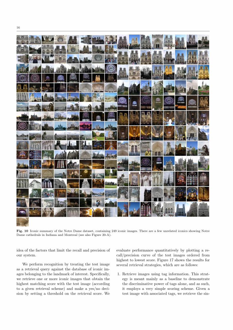
Figures 8, 9 and 10 show the sets of iconic images(iconic summaries) generated by our system from eachof the three datasets. For the most part, these sum-maries are very clean and complete, with just a fewirrelevant or ambiguous iconics. For example, the sum-mary for the Statue of Liberty dataset includes a fewiconics corresponding to views of lower Manhattan, El-lis Island, and an M&M statue that parodies the Statueof Liberty. The iconic summary of San Marco containsa few views of Castillo de San Marcos in Florida, whilethe summary for Notre Dame contains some views ofNotre Dame cathedrals in Montreal and Indiana thatdid not get removed by our tag-based filtering step (Sec-tion 3.4).

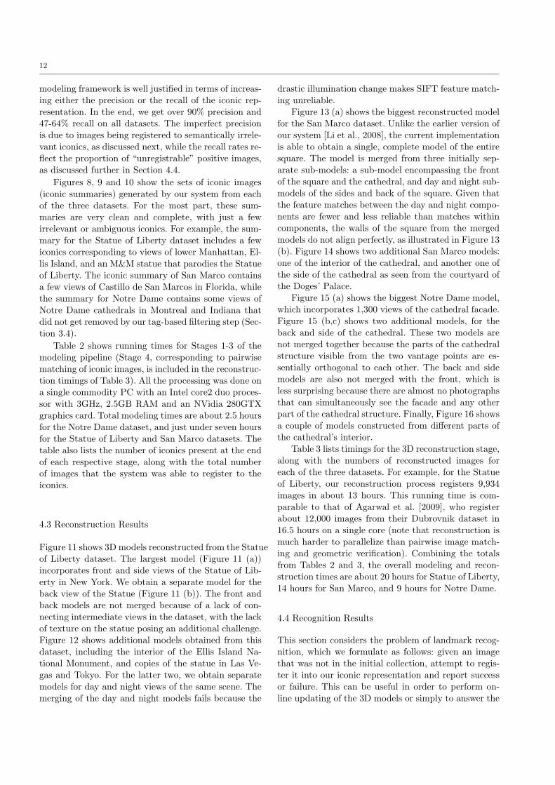
Table 2 shows running times for Stages 1-3 of themodeling pipeline (Stage 4, corresponding to pairwisematching of iconic images, is included in the reconstruc-tion timings of Table 3). All the processing was done ona single commodity PC with an Intel core2 duo proces-sor with 3GHz, 2.5GB RAM and an NVidia 280GTXgraphics card. Total modeling times are about 2.5 hoursfor the Notre Dame dataset, and just under seven hoursfor the Statue of Liberty and San Marco datasets. Thetable also lists the number of iconics present at the endof each respective stage, along with the total numberof images that the system was able to register to theiconics.

4.3 Reconstruction Results

Figure 11 shows 3D models reconstructed from the Statueof Liberty dataset. The largest model (Figure 11 (a))incorporates front and side views of the Statue of Lib-erty in New York. We obtain a separate model for theback view of the Statue (Figure 11 (b)). The front andback models are not merged because of a lack of con-necting intermediate views in the dataset, with the lackof texture on the statue posing an additional challenge.Figure 12 shows additional models obtained from thisdataset, including the interior of the Ellis Island Na-tional Monument, and copies of the statue in Las Ve-gas and Tokyo. For the latter two, we obtain separatemodels for day and night views of the same scene. Themerging of the day and night models fails because the

drastic illumination change makes SIFT feature match-ing unreliable.

Figure 13 (a) shows the biggest reconstructed modelfor the San Marco dataset. Unlike the earlier version ofour system [Li et al., 2008], the current implementationis able to obtain a single, complete model of the entiresquare. The model is merged from three initially sep-arate sub-models: a sub-model encompassing the frontof the square and the cathedral, and day and night sub-models of the sides and back of the square. Given thatthe feature matches between the day and night compo-nents are fewer and less reliable than matches withincomponents, the walls of the square from the mergedmodels do not align perfectly, as illustrated in Figure 13(b). Figure 14 shows two additional San Marco models:one of the interior of the cathedral, and another one ofthe side of the cathedral as seen from the courtyard ofthe Doges’ Palace.

Figure 15 (a) shows the biggest Notre Dame model,which incorporates 1,300 views of the cathedral facade.Figure 15 (b,c) shows two additional models, for theback and side of the cathedral. These two models arenot merged together because the parts of the cathedralstructure visible from the two vantage points are es-sentially orthogonal to each other. The back and sidemodels are also not merged with the front, which isless surprising because there are almost no photographsthat can simultaneously see the facade and any otherpart of the cathedral structure. Finally, Figure 16 showsa couple of models constructed from different parts ofthe cathedral’s interior.

Table 3 lists timings for the 3D reconstruction stage,along with the numbers of reconstructed images foreach of the three datasets. For example, for the Statueof Liberty, our reconstruction process registers 9,934images in about 13 hours. This running time is com-parable to that of Agarwal et al. [2009], who registerabout 12,000 images from their Dubrovnik dataset in16.5 hours on a single core (note that reconstruction ismuch harder to parallelize than pairwise image match-ing and geometric verification). Combining the totalsfrom Tables 2 and 3, the overall modeling and recon-struction times are about 20 hours for Statue of Liberty,14 hours for San Marco, and 9 hours for Notre Dame.

4.4 Recognition Results

This section considers the problem of landmark recog-nition, which we formulate as follows: given an imagethat was not in the initial collection, attempt to regis-ter it into our iconic representation and report successor failure. This can be useful in order to perform on-line updating of the 3D models or simply to answer the

13

0 0.2 0.4 0.6 0.8 10

0.1

0.2

0.3

0.4

0.5

0.6

0.7

0.8

0.9

1Statue of Liberty Modeling

Recall

Pre

cisi

on

Stage 1Stage 2aStage 2bStage 3Stage 4

0 0.2 0.4 0.6 0.8 10

0.1

0.2

0.3

0.4

0.5

0.6

0.7

0.8

0.9

1San Marco Modeling

Recall

Pre

cisi

onStage 1Stage 2aStage 2bStage 3Stage 4

0 0.2 0.4 0.6 0.8 10

0.1

0.2

0.3

0.4

0.5

0.6

0.7

0.8

0.9

1Notre Dame Modeling

Recall

Pre

cisi

on

Stage 1Stage 2aStage 2bStage 3Stage 4

Final Finalrecall precision

Stage 1 1.0 0.60Stage 2a 0.81 0.72Stage 2b 0.33 0.95Stage 3 0.50 0.94Stage 4 0.47 0.95





Fig. 7 Top: Recall/precision curves for modeling. Bottom: summary of final (rightmost) precision and recall values for each curve.The different stages correspond to stages 1-4 in Algorithm 1. Stage 1: Clustering using gist and ranking each image by the size ofits gist cluster (Section 3.1). Stage 2a: Geometric verification of iconics and ranking each image by the inlier number of its iconic(Section 3.2). The recall is lower because inconsistent clusters are rejected. Stage 2b: Registering each image to its iconic and rankingthe image by the number of inliers of the two-view transformation to the iconic (Section 3.2). Unlike in the first two stages, imagesare no longer arranged by cluster, but ranked individually by this score. The recall is lower because images with not enough inliersto estimate a two-view transformation are rejected. Stage 3: Images discarded in the previous stages are subject to a second roundof re-clustering and geometric verification (Section 3.3). This results in an increase in recall due to the discovery of additional iconicclusters. Stage 4: Tag information is used to discard semantically unrelated clusters (Section 3.4). Note the increase in precision dueto the removal of spurious iconics.

Feature Stage 1 Stage 2 Stage 3

extraction Gist Geometric Re-clustering Totals

Gist SIFT clustering verification and registration

Dataset Timing Timing Timing Timing Initial Timing Additional Timing Total Imageshrs:min hrs:min hrs:min hrs:min iconics hrs:min iconics hrs:min iconics registered

Liberty 0:04 2:12 0:21 0:56 260 3:21 212 6:53 454 13,888San Marco 0:04 3:18 0:19 0:24 270 2:47 195 6:52 417 12,253Notre Dame 0:01 0:57 0:03 0:22 211 1:02 81 2:25 249 3,058

Table 2 Summary statistics for the modeling stage of the processing pipeline, wherein the raw image collection is reduced to a set ofrepresentative iconic images. The table lists the time taken for each stage of processing, along with the total number of iconic imagespresent at each step. The summary column lists the final number of iconics, along with the total number of images that could beregistered to these iconics. Note that the final number of iconics reflects the results following the tag-filtering step, where some iconicsare rejected from each dataset. Specifically, this step rejects 20 iconics from the Statue of Liberty dataset, 47 from the San Marcodataset, and 43 from the Notre Dame dataset. The timing for this step is on the order of a few seconds, and is thus omitted from the

table.

question of whether the image contains the landmarkof interest. In our formulation, landmark recognition isconceptually very close to the task of registering left-over images in Stage 3 of our modeling pipeline (Sec-tion 3.3). In this section, we take a closer look at thistask with a few new goals in mind. First, a separateevaluation of recognition performance allows us to testimportant implementation choices that we have not yet

examined, such as the use of keypoint-based indexinginstead of gist descriptors for image matching. Second,it allows us to quantify the extent to which our iconicsummaries are representative of all landmark imagesmarked as positive by human observers. Third, by ex-amining individual examples of successful and unsuc-cessful recognition (Figures 18-20), we can get a better

14

Fig. 8 Iconic summary of the Statue of Liberty dataset, containing 454 iconic images. Iconic images depict copies of the Statue in NewYork, Las Vegas, and Tokyo. There are also a few technically spurious, but related iconics corresponding to views of lower Manhattan,Ellis Island, and an M&M statue that parodies the Statue of Liberty.

15

Fig. 9 Iconic summary of the San Marco dataset, containing 417 iconic images. This summary retains a few spurious iconics that did

not get rejected by our tag filtering step, including views of Castillo de San Marcos in Florida (see also Figure 20-B).

16

Fig. 10 Iconic summary of the Notre Dame dataset, containing 249 iconic images. There are a few unrelated iconics showing Notre

Dame cathedrals in Indiana and Montreal (see also Figure 20-A).

idea of the factors that limit the recall and precision ofour system.

We perform recognition by treating the test imageas a retrieval query against the database of iconic im-ages belonging to the landmark of interest. Specifically,we retrieve one or more iconic images that obtain thehighest matching score with the test image (accordingto a given retrieval scheme) and make a yes/no deci-sion by setting a threshold on the retrieval score. We

evaluate performance quantitatively by plotting a re-call/precision curve of the test images ordered fromhighest to lowest score. Figure 17 shows the results forseveral retrieval strategies, which are as follows:

1. Retrieve images using tag information. This strat-egy is meant mainly as a baseline to demonstratethe discriminative power of tags alone, and as such,it employs a very simple scoring scheme. Given atest image with associated tags, we retrieve the sin-

17

(a) Two views of the Statue of Liberty in New York (9025 cameras).

(b) The back side of the Statue of Liberty (171 cameras).

Fig. 11 Selected final models of the Statue of Liberty dataset. In this and the following model figures, the inset images give repre-

sentative views of the 3D structure covered by the model.

18

(a) The interior of the Ellis Island National Monument (73 cameras).

(b) The Statue of Liberty in Las Vegas. Left: day model (223 cameras), right: night model (148 cameras).

(c) The Statue of Liberty in Tokyo. Left: day model (146 cameras), right: night model (27 cameras).

Fig. 12 Additional models constructed from the Statue of Liberty dataset.

gle iconic image that contains the largest fraction ofthese tags. It can be seen from Figure 17 that byitself, this scheme is quite unreliable.

2. Compare the test image to the iconics using eithergist descriptors or a bag-of-features representationusing the vocabulary tree indexing scheme [Nisterand Stewenius, 2006]. In either case, the retrievalscore is the similarity (or inverse distance) betweenthe query and the single best-matching iconic. The

performance of gist descriptors is shown in Figure17 (a), and the performance of the vocabulary treeis shown in (b). For San Marco and Notre Dame,gist and vocabulary tree have roughly similar per-formance. However, for the Statue of Liberty, theperformance of the vocabulary tree is almost dis-astrous – even worse than that of the tag-basedbaseline. This is due to the relative lack of texturein many Statue of Liberty images, which gives too

19

(a) Two views of the San Marco Square model (10,338 cameras).

(b) Overhead view of the square highlighting misalignment artifacts between day and night sub-models. The two sampleviews come from different models and give rise to inconsistent structure due to a lack of direct feature matches.

Fig. 13 Biggest reconstructed 3D model for the San Marco dataset.

20

Fig. 14 Additional models reconstructed from the San Marco Square dataset. Left: the nave of the church (81 cameras). Right: the

side of the church (90 cameras).

Construction of Link discovery and Expansion of models

Dataset initial sub-models merging of sub-models with non-iconic images Total

Timing Reconstructed Timing Reconstructed Timing Reconstructed Timinghrs:min iconics hrs:min images hrs:min images hrs:min

Liberty 0:32 309 2:51 434 9:34 9,934 12:57San Marco 0:28 317 0:39 424 6:07 10,429 7:14Notre Dame 0:10 115 0:21 186 5:46 2,371 6:17

Table 3 Summary statistics of the steps of our 3D reconstruction (refer back to Section 3.5). Note that the first stage, constructionof sub-models, includes the time for finding metric reconstructions between pairs of iconics and constructing the iconic scene graph.It can be seen that significantly large datasets can be processed on the order of a few hours.

few local feature matches for the vocabulary treeto work reliably. The strong performance of globalfeatures as compared to local ones validates our im-plementation choice of relying so extensively on gistdescriptors, given that local features are often pre-ferred in image search applications [Douze et al.,2009]. Our results seem to indicate that, providedthat we query against a set of sufficiently diverseand representative views, global features will workwell for retrieval.

3. Retrieve the top k candidate iconics using eithergist or vocabulary tree and perform geometric veri-fication with each candidate as described in Section3.2. In this case, the retrieval score is the numberof inliers to a two-view transformation (homogra-phy or fundamental matrix) between the test imageand the best-matching iconic. It can be seen thatfor both kinds of descriptors, geometric verificationsignificantly improves accuracy, as does retrievingmore candidate iconics for verification (we show re-

sults for k = 1, 5, and 20). A high inlier score is astrong indication of the presence of the landmark,whereas a very low inlier score is inconclusive. Thecolored circles on the curves labeled “GIST+kNN”or “VocTree+kNN” correspond to an inlier thresh-old of 18, which represents the point up to whicha classification can be made with reasonable con-fidence. Note that this is the same threshold thatis used for geometric verification of images againsticonics during modeling (Section 3.2). We can seethat the best recall rates reached on the test setsfor this threshold are all in the 60% range, which iscomparable to the recall rates of images registeredinto the iconic representation during modeling (Fig-ure 7).

Figure 18 shows successful recognition examples forthe three datasets. It can be seen that our system isable to return a correct match in the presence of occlu-sions (18-B). In addition, in the case of almost identicallandmarks occurring in different locations, such as the

21

(a) The front side of the Notre Dame Cathedral (1300 cameras).

(b) The back side of the cathedral (487 cameras).

(c) The right side of the cathedral (94 cameras).

Fig. 15 The three largest final models of the Notre Dame dataset.

22

Fig. 16 Two models for different parts of the Notre Dame cathedral interior (118 cameras and 65 cameras, respectively).

Statue of Liberty in Tokyo (18-A), we are able matchthe test image to the correct instance of the landmark.Correct matches are also returned for some atypicalviews, such as photographs taken from inside of theNotre Dame Cathedral (18-C).

Figure 19 shows some typical false negatives wherea test image containing the landmark does not gatherenough inliers to any of the iconics. For instance, in thecase where the landmark occupies only a very smallarea of the image (19-A), neither gist descriptors norfeature-based geometric verification provide strong ev-idence in favor of the image. Artistic depictions of thelandmark (19-B) fail geometric verification, while sig-nificantly atypical views (19-C) may not have match-ing iconics. Based on the recall rates for modeling andtesting presented in Figures 7 and 17, it appears thatroughly 40% of all images labeled as positive by humanobservers fall into the above “unregistrable” categories.

As a consequence of the strong geometric constraintsenforced in our system, false positives (or images thathurt precision) are significantly less frequent. Two ex-ample cases are shown in Figure 20, where the errorarises because the set of iconic images itself containsfalse positives. For example, the iconics for the NotreDame dataset include images of the Notre Dame Basil-ica in Montreal (20-A), and the iconics for the SanMarco dataset include images of the Castillo de SanMarcos in Florida (20-B).

4.5 Browsing

As a final application of the proposed iconic scene rep-resentation, we describe how to hierarchically organizelandmark images for browsing.

Iconic scene graphs tend to contain clusters of icon-ics that have strong geometric connections among them,corresponding to dominant aspects of the landmark.

We identify these components by partitioning the graphusing normalized cuts (N-cuts) [Shi and Malik, 2000].The N-cuts algorithm requires the desired number ofcomponents to be specified as input. We have foundthat specifying 40 to 50 components produces accept-able results for all our datasets. Note that in our earlierwork [Li et al., 2008], N-cuts was also used to initializesub-models during reconstruction. Since then, we havefound that hard initial partitioning is not as conduciveto model merging as the incremental scheme of Section3.5; however, N-cuts still produce very good results forthe application of browsing.

The components of the iconic scene graph form thetop level of the browsing hierarchy. The second levelof the hierarchy consists of iconic images grouped bycomponent. The user can click on the representativeiconic of each component (which we select to be theiconic with the largest gist cluster) to “expand” thecomponent and see all the iconic images that belong toit. The third level consists of all remaining non-iconicimages in the dataset grouped by the iconic of their gistcluster. During interactive browsing, each iconic imagecan be expanded to show all the images from its cluster,which will all tend to be very similar in appearance tothe iconic. Figure 21 gives a snapshot of this three-levelorganization for the Statue of Liberty dataset. All threedatasets can be browsed interactively on our website9.

5 Conclusion

In this article, we have presented a scalable, unified so-lution to the problems of dataset collection, scene sum-marization, browsing, 3D reconstruction, and recogni-tion for landmark image collections gathered from theInternet. By efficiently combining 2D appearance cueswith 3D geometric constraints, we are able to robustly

9 www.cs.unc.edu/PhotoCollectionReconstruction

23

(a) (b)

0 0.2 0.4 0.6 0.8 10

0.1

0.2

0.3

0.4

0.5

0.6

0.7

0.8

0.9

1Statue of Liberty Testing − GIST

Recall

Pre

cisi

on

TagGIST 1NNGIST 1NN + MatchGIST 5NN + MatchGIST 20NN + Match

0 0.2 0.4 0.6 0.8 10

0.1

0.2

0.3

0.4

0.5

0.6

0.7

0.8

0.9

1Statue of Liberty Testing − VocTree

RecallP

reci

sion

TagVocTree 1NNVocTree 1NN + MatchVocTree 5NN + MatchVocTree 20NN + Match

0 0.2 0.4 0.6 0.8 10

0.1

0.2

0.3

0.4

0.5

0.6

0.7

0.8

0.9

1

Recall

Pre

cisi

on

San Marco Testing − GIST


0 0.2 0.4 0.6 0.8 10

0.1

0.2

0.3

0.4

0.5

0.6

0.7

0.8

0.9

1

Recall

Pre

cisi

on

San Marco Testing − VocTree


0 0.2 0.4 0.6 0.8 10

0.1

0.2

0.3

0.4

0.5

0.6

0.7

0.8

0.9

1Notre Dame Testing − GIST

Recall

Pre

cisi

on


0 0.2 0.4 0.6 0.8 10

0.1

0.2

0.3

0.4

0.5

0.6

0.7

0.8

0.9

1

Recall

Pre

cisi

on

Notre Dame Testing − VocTree


Fig. 17 Recall/precision curves for testing. The different retrieval strategies are as follows. GIST 1NN (resp. VocTree 1NN):retrieval of the single nearest iconic using the gist descriptor (resp. vocabulary tree); GIST kNN+Match (resp. VocTreekNN+Match): retrieval of k nearest exemplars using gist (resp. vocabulary tree) followed by geometric verification; Tag: tag-basedranking. The colored circles on the curves correspond to an inlier threshold of 18.

24

�

��

��

��

�

�

��

��

��

��

��

��

��

��

Fig. 18 An illustration of one successful case for image retrieval for each dataset. In each of the examples A-C, the query image is onthe left. On the right, the top row shows the top five iconics closest to the query in terms of gist distance, re-ranked by the numberof inliers to an estimated two-view transformation. As discussed in the text, inlier threshold of 18 corresponds to reliable registration.The bottom row shows analogous results for the closest five iconics according to the vocabulary tree score.

deal with the significant amount of clutter present incommunity-contributed photo collections. Our imple-mented system can process up to fifty thousand imageson a single commodity PC in roughly a day. While thereremains much scope for further optimization, this al-ready represents an order of magnitude improvementover existing techniques that do not make use of cloudcomputing.

A number of interesting research challenges remainopen. In order to further scale our system, we need tobe able to perform the initial gist clustering step in

memory for much larger datasets. To this end, we arecurrently exploring techniques for compressing gist de-scriptors to short binary strings whose Hamming dis-tances approximate Euclidean distances in the originalfeature space [Torralba et al., 2008].

Currently, we assume that the iconic scene graph issmall enough (a few hundred iconic images), so that itcan be computed by exhaustive pairwise matching oficonics and traversed exhaustively during SfM. Scalingto much larger graphs will require feature-based index-ing of iconic images, as well as graph simplification tech-

25

GIST

Vocabulary Tree

Query

GIST

Vocabulary Tree

Query

A

B

GIST

Vocabulary Tree

Query

C

Score: 7 Score: 9 Score: 9 Score: 9 Score: 7






Fig. 19 Typical false negatives, or test images that could not be reliably registered to any of the iconics. The layout of the figure isthe same as that of Figure 18.

niques similar to those of Snavely et al. [2008a]. It mayalso necessitate the development of efficient out-of-corebundle adjustment techniques similar to [Ni et al., 2007]that use the connectivity of the iconic scene graph.

One of the limitations of our current system actuallystems from its greatest source of efficiency, namely, itsreliance on iconic images. By definition, iconic imagescorrespond to “popular” viewpoints from which manypeople take photos of a landmark. While this helps indrastically reducing the redundancy that is present incommunity photo collections, it can pose difficultieswhen merging two 3D sub-models, where non-iconicviews may be required to provide the intermediate con-

nections. While the link discovery method described inSection 3.5 is able to recover some missing links, it isnot always successful. In the future, we plan to workon improved link discovery algorithms that use moresophisticated image retrieval techniques such as queryexpansion to find rare connecting views.

Illumination changes pose another major challengefor modeling and recognition. In fact, as discussed inSection 4, one of the biggest causes of failure for 3Dmodel merging is a difference in the lighting betweenthe two components (i.e., day vs. night). Methods forillumination modeling like those of Haber et al. [2009]may help in addressing this problem.

26

GIST

Vocabulary Tree

Query

GIST

Vocabulary Tree

Query

A

B





Fig. 20 An illustration of the less common case of false positives in landmark recognition. In both examples, the error arises isdue to the presence of an iconic image that represents a different, though similarly named landmark. The top matching iconic in Acorresponds to the Notre Dame Basilica in Montreal, while the matching iconic in B is of the Castillo de San Marcos in Florida.

Level 1Level 2

Level 3

Fig. 21 Hierarchical organization of the dataset for browsing. Level 1: components of the iconic scene graph. Level 2: Each componentcan be expanded to show all the iconic images associated with it. Level 3: each iconic can be expanded to show the images associatedwith its gist cluster. Our three datasets may be browsed online at www.cs.unc.edu/PhotoCollectionReconstruction.

27

Acknowledgments

This research was supported in part by DARPA AS-SIST program, NSF grants IIS-0916829, IIS-0845629,and CNS-0751187, and other funding from the U.S.government. Svetlana Lazebnik was supported by theMicrosoft Research Faculty Fellowship. We would alsolike to thank our collaborators Marc Pollefeys, XiaoweiLi, Christopher Zach, and Tim Johnson.

References

Sameer Agarwal, Noah Snavely, Ian Simon, Steven M.Seitz, and Richard Szeliski. Building Rome in a day.In ICCV, 2009.

S. Arya, D. Mount, N. Netanyahu, R. Silverman, andA. Wu. An optimal algorithm for approximate near-est neighbor searching fixed dimensions. In JACM,volume 45, pages 891–923, 1998.

C. Beder and R. Steffen. Determining an initial imagepair for fixing the scale of a 3d reconstruction froman image sequence. In Proc. DAGM, pages 657–666,2006.

T. L. Berg and D.A. Forsyth. Automatic ranking oficonic images. Technical report, University of Cali-fornia, Berkeley, 2007.

Tamara L. Berg and Alexander C. Berg. Finding iconicimages. In The 2nd Internet Vision Workshop atIEEE Conference on Computer Vision and PatternRecognition, 2009.

T.L. Berg and D.A. Forsyth. Animals on the web. InCVPR, 2006.

V. Blanz, M. Tarr, and H. Bulthoff. What object at-tributes determine canonical views? Perception, 28(5):575–600, 1999.

O. Chum, J. Philbin, J. Sivic, M. Isard, and A. Zisser-man. Total recall: Automatic query expansion witha generative feature model for object retrieval. InICCV, 2007.

B. Collins, J. Deng, L. Kai, and L. Fei-Fei. Towardsscalable dataset construction: An active learning ap-proach. In ECCV, 2008.

T. Denton, M. Demirci, J. Abrahamson, A. Shokoufan-deh, and S. Dickinson. Selecting canonical views forview-based 3-d object recognition. In ICPR, pages273–276, 2004.

Matthijs Douze, Herve Jegou, Harsimrat Sandhawalia,Laurent Amsaleg, and Cordelia Schmid. Evaluationof gist descriptors for web-scale image search. InInternational Conference on Image and Video Re-trieval, 2009.

Rob Fergus, Pietro Perona, and Andrew Zisserman. Avisual category filter for Google images. In ECCV,2004.

J.-M. Frahm and M. Pollefeys. RANSAC for (quasi-)degenerate data (QDEGSAC). In CVPR, volume 1,pages 453–460, 2006.

Tom Haber, Christian Fuchs, Philippe Bekaert, Hans-Peter Seidel, Michael Goesele, and Hendrik P.A.Lensch. Relighting objects from image collections.In Proceedings of CVPR, 2009.

P. Hall and M. Owen. Simple canonical views. InBMVC, pages 839–848, 2005.

James Hays and Alexei A. Efros. Scene completionusing millions of photographs. In SIGGRAPH, 2007.

Yushi Jing and Shumeet Baluja. Visualrank: ApplyingPageRank to large-scale image search. PAMI, 30:1877–1890, 2008.

L. Kennedy, S.-F. Chang, and I. Kozintsev. To search orto label?: Predicting the performance of search-basedautomatic image classifiers. In ACM Multimedia In-formation Retrieval Workshop (MIR 2006), 2006.

Lyndon Kennedy and Mor Naaman. Generating diverseand representative image search results for land-marks. In Proceedings of the Seventeenth Interna-tional World Wide Web Conference (WWW 2008),2008.

Li-Jia Li, Gang Wang, and Li Fei-Fei. Optimol: auto-matic object picture collection via incremental modellearning. In CVPR, 2007.

X. Li, C. Wu, C. Zach, S. Lazebnik, and J.-M. Frahm.Modeling and recognition of landmark image collec-tions using iconic scene graphs. In ECCV, 2008.

Yunpeng Li, David J. Crandall, and Daniel P. Hutten-locher. Landmark classification in large-scale imagecollections. In ICCV, 2009.

D. Lowe. Distinctive image features from scale-invariant keypoints. IJCV, 60(2):91–110, 2004.

Kai Ni, Drew Steedly, and Frank Dellaert. Out-of-corebundle adjustment for large-scale 3d reconstruction.In ICCV, 2007.

D. Nister. An efficient solution to the five-point relativepose problem. PAMI, 26(6):756–770, 2004.

D. Nister and H. Stewenius. Scalable recognition witha vocabulary tree. In CVPR, 2006.

Aude Oliva and Antonio Torralba. Modeling the shapeof the scene: a holistic representation of the spatialenvelope. IJCV, 42(3):145–175, 2001.

S. Palmer, E. Rosch, and P. Chase. Canonical perspec-tive and the perception of objects. Attention andPerformance, IX:135–151, 1981.

J. Philbin and A. Zisserman. Object mining using amatching graph on very large image collections. InProceedings of the Indian Conference on Computer

28

Vision, Graphics and Image Processing, 2008.J. Philbin, O. Chum, M. Isard, J. Sivic, and A. Zis-

serman. Lost in quantization: Improving particularobject retrieval in large scale image databases. InCVPR, 2008.

Rahul Raguram and Svetlana Lazebnik. Computingiconic summaries of general visual concepts. In Work-shop on Internet Vision CVPR, 2008.

Rahul Raguram, Jan-Michael Frahm, and Marc Polle-feys. A comparative analysis of RANSAC techniquesleading to adaptive real-time random sample consen-sus. In ECCV, 2008.

Frederik Schaffalitzky and Andrew Zisserman. Multi-view matching for unordered image sets, or ”how do iorganize my holiday snaps?”. In ECCV ’02: Proceed-ings of the 7th European Conference on ComputerVision-Part I, pages 414–431, 2002.

F. Schroff, A. Criminisi, and A. Zisserman. Harvestingimage databases from the web. In ICCV, 2007.

J. Shi and J. Malik. Normalized cuts and image seg-mentation. PAMI, 22(8):888–905, 2000.

B. Sigurbjornsson and R. van Zwol. Flickr tag recom-mendation based on collective knowledge. In WWW,2008.

Ian Simon, Noah Snavely, and Steven M. Seitz. Scenesummarization for online image collections. In ICCV,2007.

N. Snavely, S. M. Seitz, and R. Szeliski. Skeletal setsfor efficient structure from motion. In CVPR, 2008a.

N. Snavely, S. M. Seitz, and R. Szeliski. Modeling theworld from Internet photo collections. InternationalJournal of Computer Vision, 80(2):189–210, Novem-ber 2008b.

Noah Snavely, Steven M. Seitz, and Richard Szeliski.Photo tourism: Exploring photo collections in 3d. InSIGGRAPH, pages 835–846, 2006.

Susan Sontag. On Photography. Penguin, 1977.A. Torralba, R. Fergus, and Y. Weiss. Small codes and

large databases for recognition. In CVPR, 2008.D. Weinshall, M. Werman, and Y. Gdalyahu. Canonical

views, or the stability and likelihood of images of 3dobjects. In Image Understanding Workshop, 1994.

Yan-Tao Zheng, Ming Zhao, Yang Song, H. Adam,U. Buddemeier, A. Bissacco, F. Brucher, Tat-SengChua, and H. Neven. Tour the world: Building aweb-scale landmark recognition engine. In CVPR,2009.

Modeling and Recognition of Landmark Image Collections Using

Documents

Transcript of Modeling and Recognition of Landmark Image Collections Using