Modeling and Inversion of Self-Potential Data

Modeling and Inversion of Self-Potential Data

by

Burke J. Minsley

B.S. Applied Physics, Purdue University, 1997

Submitted to the Department of Earth, Atmospheric, and Planetary Sciences

in partial fulfillment of the requirements for the degree of

Doctor of Philosophy

at the

MASSACHUSETTS INSTITUTE OF TECHNOLOGY

June 2007

© Massachusetts Institute of Technology, 2007. All rights reserved.

Author .……………………………………………………………………..

Department of Earth, Atmospheric, and Planetary Sciences 23 May 2007

Certified by .………………………………………………………………..

Frank Dale Morgan Professor of Geophysics

Thesis Supervisor

Accepted by .……………………………………………………………….

Maria T. Zuber E.A. Griswold Professor of Geophysics

Head, Department of Earth, Atmospheric and Planetary Sciences

3

Modeling and Inversion of Self-Potential Data by

Burke J. Minsley

Submitted to the Department of Earth, Atmospheric, and Planetary Sciences on 23 May 2007, in partial fulfillment of the

requirements for the Degree of Doctor of Philosophy in Geophysics

Abstract

This dissertation presents data processing techniques relevant to the acquisition, mod-eling, and inversion of self-potential data. The primary goal is to facilitate the inter-pretation of self-potentials in terms of the underlying mechanisms that generate the measured signal. The central component of this work describes a methodology for inverting self-potential data to recover the three-dimensional distribution of causative sources in the earth. This approach is general in that it is not specific to a particular forcing mechanism, and is therefore applicable to a wide variety of problems. Self-potential source inversion is formulated as a linear problem by seeking the distribution of source amplitudes within a discretized model that satisfies the meas-ured data. One complicating factor is that the potentials are a function of the earth resistivity structure and the unknown sources. The influence of imperfect resistivity information in the inverse problem is derived, and illustrated through several syn-thetic examples. Source inversion is an ill-posed and non-unique problem, which is addressed by incorporating model regularization into the inverse problem. A non-traditional regu-larization method, termed “minimum support,” is utilized to recover a spatially com-pact source model rather than one that satisfies more commonly used smoothness con-straints. Spatial compactness is often an appropriate form of prior information for the inverse source problem. Minimum support regularization makes the inverse problem non-linear, and therefore requires an iterative solution technique similar to iteratively re-weighted least squares (IRLS) methods. Synthetic and field data examples are studied to illustrate the efficacy of this method and the influence of noise, with appli-cations to hydrogeologic and electrochemical self-potential source mechanisms. Finally, a novel technique for pre-processing self-potential data collected with ar-bitrarily complicated survey geometries is presented. This approach overcomes the inability of traditional processing methods to produce a unique map of the potential field when multiple lines of data form interconnected loops. The data are processed simultaneously to minimize mis-ties on a survey-wide basis using either an l2 or l1 measure of misfit, and simplifies to traditional methods in the absence of survey com-plexity. The l1 measure requires IRLS solution methods, but is more reliable in the presence of data outliers.

Thesis Supervisor: Frank Dale Morgan Title: Professor of Geophysics

5

Biography

The author, Burke Minsley, was born in New York City on July 13, 1975. He at-

tended Purdue University from 1993 to 1997, and received a Bachelors degree in Ap-

plied Physics with a minor in Mathematics. His first introduction to geophysics came

as an undergraduate student, but only became a serious topic of interest during his

employment with Schlumberger WesternGeco as a field geophysicist working off-

shore on seismic research vessels from 1997 to 2002. He moved to Massachusetts in

1999, and subsequently enrolled as a graduate student in geophysics at MIT in the fall

of 2002.

The author currently lives in Cambridge, Massachusetts with his wife, Caron, and

dog, Cedar.

Education

• B.S. Applied Physics with Mathematics minor, Purdue University. May 1997.

Employment

• Research Assistant, Department of Earth, Atmospheric, and Planetary Sci-ences, Massachusetts Institute of Technology. August 2002 - present.

• Field Geophysicist, Schlumberger WesternGeco. August 1997 – June 2002.

• Teaching Assistant, Physics Department, Purdue University. January – May 1997.

Awards

• Outstanding Student Paper Award, Near Surface Geophysics, Fall AGU. 2006. • NSF student travel award: biogeophysics session at Spring AGU. May 2005.

• Martin Family Society Fellowship for Sustainability. 2004 – 2005.

6

Refereed publications

• Ajo-Franklin, J.B., B.J. Minsley, and T. Daley (2007), Applying compactness constraints to differential traveltime tomography, Geophysics, in press.

• Minsley, B., J. Sogade, and F.D. Morgan (2007), Three-dimensional self-potential inversion for subsurface DNAPL contaminant detection at the Savan-nah River Site, South Carolina, Water Resour. Res., 43, W04429, doi:10.1029/2005WR03996.

• Minsley, B., J. Sogade, and F.D. Morgan (2007), 3D source inversion of self-potential data, J. Geophys. Res., 112, B02202, doi:10.1029/2006JB004262.

• Willis, M.E., D.R. Burns, R. Rao, B. Minsley, M.N. Toksöz, and L. Vetri (2006), Spatial orientation and distribution of reservoir fractures from scat-tered seismic energy, Geophysics, 71(5), 43-51, doi:10.1190/1.2235977.

Publications in preparation

• Minsley, B., J. Ajo-Franklin, M. Al-Otaibi, A. Mukhopadhyay, F. Al-Ruwaih, and F.D. Morgan, Modeling the hydrogeophysical response of aquifer storage and recovery in Kuwait.

• Minsley, B., W. Rodi, and F.D. Morgan, Quantifying the effects of unknown resistivity structure on self-potential inversion.

• Minsley, B., D. Coles, Y. Vichabian, and F.D. Morgan, Accounting for mis-ties on self-potential surveys with complicated acquisition geometries.

• Vichabiain, Y., B. Minsley, D. Coles, and F.D. Morgan, Self-potential and gravity surveys for geothermal exploration in Nevis.

Conference abstracts, reports, and presentations

• Minsley, B. and F.D. Morgan (2006), Quantifying the effects of unknown re-sistivity structure on self-potential inversion, EOS Trans. AGU, 87(52), Fall Meet. Suppl., Abstract NS31A-1562, POSTER - San Francisco, CA.

• Minsley, B., J. Ajo-Franklin, M. Al-Otaibi, A. Mukhopadhyay, F. Al-Ruwaih, and F.D. Morgan (2006), Modeling the hydrogeophysical response of aquifer storage and recovery in Kuwait, SEG Summer Research Workshop on Hydro-geophysics, Vancouver, Canada.

• Minsley, B., J.B. Ajo-Franklin, and F.D. Morgan (2006), Non-linear Con-straints with Application to Self-Potential Source Inversion, Earth Resources Laboratory Annual Consortium Report, Cambridge, MA.

• Ajo-Franklin, J.B., B. Minsley, and T.M. Daley (2006), Applying Compact-ness Constraints to Seismic Traveltime Tomography, Earth Resources Labora-tory Annual Consortium Report, Cambridge, MA.

• Minsley, B., J. Sogade, and F.D. Morgan (2005), Source inversion of self-potential data with compactness constraints, EOS Trans. AGU, 86(52), Fall Meet. Suppl., Abstract H13C-1347, POSTER - San Francisco, CA.

7

• Ajo-Franklin, J.B. and B. Minsley (2005), Application of minimum support constraints to seismic traveltime tomography, EOS Trans. AGU, 86(52), Fall Meet. Suppl., Abstract H13C-1344, POSTER - San Francisco, CA.

• Minsley, B., J. Sogade, and F.D. Morgan (2005), Source inversion of self-potential data with compactness constraints, EOS Trans. AGU, 86(52), Fall Meet. Suppl., Abstract H13C-0147, POSTER - San Francisco, CA.

• Minsley, B.J., J. Sogade, Y. Vichabian, and F.D. Morgan (2005), 3D Self-Potential Inversion for Monitoring DNAPL Contaminant Distributions, EOS Trans. AGU, 86(18), Jt. Assem. Suppl., Abstract NS44A-02. New Orleans, LA.

• Vichabian, Y., F.D. Morgan, B. Minsley, D. Coles, and M. Krasovec (2005), Self Potential and Gravity Study for Geothermal Exploration of Nevis, EOS Trans. AGU, 86(18), Jt. Assem. Suppl., Abstract V13B-10. New Orleans, LA.

• Burns, D.R., M.E. Willis, B.J. Minsley, and M.N. Toksöz (2004), Characteriz-ing subsurface fractures from reflected and scattered seismic energy, 7th SEGJ International Symposium, Sendai, Japan.

• Minsley, B., M. Willis, M. Krasovec, D. Burns, and M.N. Toksöz (2004), In-vestigation of a fractured reservoir using P-wave AVOA analysis: a case study of the Emilio Field with support from synthetic examples, SEG 74th annual meeting, Denver, CO.

• Minsley, B., M.E. Willis, M. Krasovec, D.R. Burns, and M.N. Toksöz (2004), Fracture Detection using Amplitude versus Offset and Azimuth Analysis of a 3D P-wave Seismic Dataset and Synthetic Examples, Earth Resources Labora-tory Annual Consortium Report.

• Willis, M.E., F. Pearce, D.R. Burns, J. Byun, and B. Minsley (2004), Reservoir fracture orientation and density from reflected and scattered seismic energy, EAGE 66th annual meeting, Paris, France.

• Minsley, B., J. Sogade, V. Briggs, M. Lambert, P. Reppert, D. Coles, J. Ross-abi, B. Riha, W. Shi, and F.D. Morgan (2004), Three Dimensional Self-Potential Inversion For Subsurface Contaminant Detection and Mapping At The DOE Savannah River Site, South Carolina, SAGEEP annual meeting, Colorado Springs, CO.

• Minsley, B., J. Sogade, V. Briggs, M. Lambert, P. Reppert, D. Coles, J. Ross-abi, B. Riha, W. Shi, and F.D. Morgan (2003), 3D Inversion of a Self-Potential Dataset for Contaminant Detection and Mapping, EOS Trans. AGU, 84(46), Fall Meet. Suppl., Abstract H31B-0462. POSTER – San Francisco, CA.

• Briggs, V., J. Sogade, B. Minsley, M. Lambert, D. Coles, P. Reppert, D. Coles, F.D. Morgan, J. Rossabi, and B. Riha (2003), 3D Inversion of Induced Polari-zation Data From Borehole Measurements to Map Subsurface Contaminations of Tetrachloroethylene and Trichloroethylene, EOS Trans. AGU, 84(46), Fall Meet. Suppl., Abstract H31B-0461. POSTER – San Francisco, CA.

8

• Minsley, B., D. Burns, and M.N. Toksöz (2003), Fractured Reservoir Charac-terization using Azimuthal AVO, Earth Resources Laboratory Annual Consor-tium Report, Cambridge, MA.

• Willis, M., D. Burns, R. Rao, and B. Minsley (2003), Characterization of Scat-tered Waves from Fractures by Estimating the Transfer Function between Re-flected Events Above and Below Each Interval, Earth Resources Laboratory Annual Consortium Report, Cambridge, MA.

• Buttles, J., B. Minsley, W. Schweller, and J. Grotzinger (2001), An Experi-mental Study of Turbidite Channel Deposits: Implications for Channel Evolu-tion and Sandstone Deposits, Earth Resources Laboratory Annual Consortium Report, Cambridge, MA.

10

Acknowledgements

A primary goal in coming to MIT was to broaden my experiences as a scientist by

gaining exposure to a variety of research areas. While I never could have predicted

the path that this would take me, I think that my path has been both productive and

enlightening. Much of this can be attributed to Nafi Toksöz, my initial advisor, and

Dale Morgan, my current thesis advisor. I am grateful to both of them for their pa-

tience and willingness to let me find, and follow through with, my own research di-

rection, as this may be equally as important as the research itself. Along the way, they

both also provided generous exposure to research and experiences outside of my dis-

sertation topic.

I remember one of my earlier conversations with Dale, whom I had asked if I

could work with on one of my general exam projects. He came back to me with the

offer to work on the self-potential component of a larger field study, which would be

a nicely contained research project. I don’t think either of us had a clue that this pro-

ject would ultimately develop into my thesis topic, and it is now Chapter 5 in this dis-

sertation. Since this unexpected beginning, Dale has been a good mentor and friend,

and is always ready to provide interesting insights into nearly any topic.

My experience at the Earth Resources Laboratory has benefited from the guidance

of, and interaction with, many of the lab’s staff and researchers: Dan Burns, Mark

Willis, Rama Rao, Rob Reilinger, John Sogade, and Bill Rodi. My conversations with

Bill regarding various aspects of inverse problems were always fruitful, and often led

to new ideas in my research. John was a great resource on many thesis-related topics,

and I definitely benefited from our work together. Dan was one of my first ERL/MIT

contacts, and I am grateful for his advice throughout my time here. Any acknowl-

11

edgement to the people at ERL would not be complete without recognizing the role

played by Liz Henderson and Sue Turbak in keeping the lab organized and operating.

Also, thanks to Linda Meinke for her unending dedication to the administration of the

lab’s computer resources.

Funding for my graduate studies came from various sources, with significant sup-

port from the ERL Founding Member Consortium, the Kuwait-MIT Center for Natu-

ral Resources and the Environment, the Martin Family Society of Fellows for Sus-

tainability, and various Department of Energy grants.

Many thanks go to the faculty and lecturers from whom I took classes: Brad

Hager, Gilbert Strang, Nafi Toksöz, Bob Burridge, Brian Evans, Carl Wunsch, Dale

Morgan, Charles Harvey, Joe Ferreira, Rob van der Hilst, David Mohrig, Jeff Tester,

Michael Golay, Liz Drake, Stéphane Rondenay, and Jin Kong. Particularly to Profes-

sors Strang and Kong, whose lectures were often extremely insightful, and of quality

that one does not often see. Also, to the members of my thesis committee: Nafi Tok-

söz (chair), Dale Morgan (advisor), Dan Rothman, Bill Rodi, and Lee Slater (external

reviewer).

On a day-to-day basis, my time at MIT was most influenced by the students and

postdocs at ERL. Special thanks go to Victoria Briggs (my officemate of four years),

Darrell Coles, Samantha Grandi, Jonathan Ajo-Franklin, Xander Campmann, Youshun

Sun, and Maggie Benoit, with whom I enjoyed many discussions on all aspects of

work and life. Many others have been good friends and colleagues over the past five

years, including Hussam Busfar, Jim Buttles, Joongmoo Byun, Shihong Chi, Felix

Hermann, Xiaoxun Huang, Jonathan Kane, Mary Krasovec, Sadi Kuleli, Mike Lam-

bert, Lisa Lassner, Xu Li, Rongrong Lu, Sophie Michelet, Fred Pearce, Phil Reppert,

Sudip Sarkar, Fuxian Song, Edmond Sze, Yervant Vichabian, Xin Zhan, Yang Zhang,

Yibeng Zheng, and Zhenya Zhu.

And to all the other pieces of life that made my time at MIT more enjoyable: The

Muddy Charles, Red Sox baseball (which I am watching as I write this paragraph),

archive.org, sailing on the Charles River and Aleida, working in the MIT hobby shop,

the White Mountains, and the Waltham Fields Community Farm, to name a few.

12

Life away from campus in Inman Square has also been an important part of my

time as a graduate student, and has played a significant role in my sanity and happi-

ness during these years. Much of this can be attributed to the good friends I have

made here- Dave Granger, Chrissy Foot, Jared Shaw, Annaliese Franz, and Chris and

Allison Tonelli.

Of course I am grateful to my parents for their support and interest in my work

throughout my educational career. My mother was always happy and willing to

proofread any of my papers, even without knowing much about the topic; a very valu-

able resource. It is their support and upbringing that has allowed me to achieve what

I have.

Next-to-last is Cedar, a great companion and friend who is always there to cheer

me up, and is unfailingly happy at whatever time I come home. And finally to Caron,

who gracefully put up with my working too much and going on field trips to far-off

places. I am lucky to have her with me throughout this journey.

14

Contents

1 Introduction ........................................................................................................31

1.1 Motivation and overview of previous research ...........................................31

1.2 Outline of thesis .........................................................................................35

2 Self-potential background ..................................................................................41

2.1 Overview of the origin of self-potentials ....................................................41

2.1.1 Streaming potentials and the Helmholtz-Smoluchowski equation 44

2.1.2 Diffusion potentials and the Nernst equation ...............................51

2.1.3 Electrochemical potentials associated with redox processes ........54

2.2 Self-potential sources .................................................................................59

2.3 Synthetic self-potential response for aquifer storage and recovery (ASR) .61

3 Self-potential source inversion...........................................................................81

3.1 Introduction ................................................................................................81

3.2 The electric forward problem .....................................................................83

3.3 The inverse problem ...................................................................................85

3.4 Sensitivity scaling ......................................................................................87

3.5 Model regularization for self-potential source inversion ............................89

3.5.1 Total variation regularization .......................................................90

3.5.2 Spatially compact sources using minimum support regularization92

3.5.3 The role of multiple regularization parameters ............................95

3.5.4 Synthetic illustration of various regularization techniques...........97

3.6 3D synthetic example with minimum support regularization....................100

3.6.1 Effect of unknown resistivity structure ......................................102

3.7 Field data example....................................................................................103

15

3.8 Discussion and conclusions ......................................................................108

4 Quantifying the effect of resistivity uncertainty on self-potential data analysis127

4.1 Introduction ..............................................................................................127

4.2 Background ..............................................................................................128

4.2.1 Self-potential sources .................................................................128

4.2.2 Description of the forward and inverse problems.......................130

4.3 Deriving the effect of resistivity assumptions on the forward problem ....132

4.4 The influence of resistivity uncertainty on self-potential source inversion136

4.4.1 1D resistivity structures .............................................................137



4.4.4 Partially known resistivity structure...........................................141

4.5 Conclusions ..............................................................................................143

5 Three dimensional self-potential inversion for DNAPL contaminant detection

at the Savannah River Site, South Carolina .........................................................154

5.1 Introduction ..............................................................................................154

5.2 Background ..............................................................................................156

5.2.1 A-14 Outfall ...............................................................................156

5.2.2 Contaminants as self-potential sources ......................................157

5.3 Electrode and survey design .....................................................................159

5.3.1 Electrode design.........................................................................159

5.3.2 Survey layout .............................................................................160

5.4 Acquired data ...........................................................................................161

5.4.1 Self-potential..............................................................................161

5.4.2 Resistivity ..................................................................................162

5.5 Inversion of field data ..............................................................................163

5.6 Comparison with ground-truth data ..........................................................164

5.7 Conclusions and future work ....................................................................166

5.8 Acknowledgements ..................................................................................167

6 Accounting for mis-ties on self-potential surveys with complicated acquisition

geometries ...............................................................................................................181

16

6.1 Introduction ..............................................................................................181

6.2 Self-potential data acquisition ..................................................................182

6.3 Methodology ............................................................................................184

6.4 Application to a synthetic example using the l1 norm...............................188

6.5 Self-potential field example from Nevis, West Indies...............................191

6.6 Conclusions and future work ....................................................................193

6.7 Acknowledgements ..................................................................................194

7 Conclusions and future research directions ....................................................205

7.1 Conclusions ..............................................................................................205

7.2 Future research ideas: secondary source imaging .....................................207

Appendix A Discretization using the transmission network equations........... 211

Appendix B Minimization using an l1 measure of data misfit .........................218

Appendix C Construction notes for Ag-AgCl porous pot electrodes...............222

C.1 Ag-AgCl conductor preparation ...............................................................222

C.2 Electrode housing preparation ..................................................................223

C.3 Electrode tube and end cap .......................................................................223

C.4 Preparing the electrolyte and sealing the electrode...................................225

References...................................................................................................................... 235

18

List of Figures

Figure 1-1: Number of publications per year with topic “self-potential” based on a search of the Thomson ISI Web of Knowledge database. N.B: related terms such as “spontaneous potential” or “electrokinetic” were not searched due to a large number of hits from non-geophysical applications.................................39

Figure 2-1: Coupled forces and fluxes [adapted from Wurmstich, 1995; Bader, 2005] (top). Pictorial representation of the coupling of flows and the development of counter forces in a system [from Marshall and Madden, 1959] (bottom). ......65

Figure 2-2: Schematic of the electrical double layer in the vicinity of a solid-fluid interface. The negatively charged solid surface is balanced by fixed positive ions within the Helmholtz layer, and a diffuse layer of ions farther from the interface (top). The potential as a function of distance from the fluid-solid interface decays exponentially in the diffuse layer (bottom). ..........................66

Figure 2-3: Cross-section of a cylindrical pore (length l, radius a) with Poiseuille flow due a hydraulic pressure difference ( P∆ ) from top to bottom. The streaming current ( kj ) due to drag of excess charge is balanced by a conduction current ( cj ) in the opposite direction, resulting in an electric potential difference ( V∆ ) across the cylinder. ................................................67

Figure 2-4: Model geometries and boundary conditions for synthetic electrokinetic coupling examples. A) fluid and electric flows are confined to the same domain, where fluid flow is caused by an applied pressure difference across the sample. B) An electrically conductive layer is added to the model, but fluid flow is restricted to the same domain as A). ...........................................68

Figure 2-5: Results of electrokinetic coupling for the model in Figure 2-4a. Surface colors show the electric potentials, and contours denote lines of constant pressure. Arrows showing the streaming current, kj , in (A) are balanced everywhere by the conduction current, cj , in (B) such that the total current density is zero everywhere (C)........................................................................69

19

Figure 2-6: Results of electrokinetic coupling for the model in Figure 2-4b with -1(2) 0.01 S mr rσ σ= = ⋅ . Surface colors show the electric potentials, and

contours denote lines of constant pressure. Arrows showing the streaming current, kj , in the lower portion of the model (A) are balanced by the conduction current, cj , in the entire domain (B) such that the total current density in (C) through any vertical slice is zero, but is non-zero at any given location. ..........................................................................................................70





Figure 2-9: Maximum electric potential drop across the model in Figure 2-4b for a fixed applied hydraulic pressure difference as a function of the upper-to-lower layer conductivity ratio. The limiting case where the upper layer conductivity becomes small produces the potential difference predicted by equation (2.26).........................................................................................................................73

Figure 2-10: (A) Schematic of a Galvanic cell that can spontaneously produce a current through an external load (Rcell) due to the difference in equilibrium potential of the different metals. (B) Schematic of a corrosion cell that can spontaneously produce a current due to differences in ionic concentration or oxygen availability in the electrolyte near the top and bottom of the metal. ...74

Figure 2-11: Self-potential model surrounding an ore body from Sato and Mooney [1960, Fig. 2]. .................................................................................................75

Figure 2-12: Porosity model for the synthetic aquifer storage and recovery hydrogeophysical modeling. The geometry, aquifer properties, and injection parameters are an approximation for the planned ASR experiment in Kuwait.........................................................................................................................76

20

Figure 2-13: Modeled bulk electrical resistivity before (A) and after 12 months of (B) fresh water injection into the Dammam aquifer. Background variations in resistivity are due to the use of Archie’s Law to compute bulk resistivity from fluid resistivity and porosity............................................................................77

Figure 2-14: Individual terms describing the self-potential sources from equation (2.50) for the aquifer injection model. The major contribution to the source comes from the fluid injection at the well, rather than flow across boundaries in the coupling coefficient...............................................................................78

Figure 2-15: Self-potential response at the surface of the aquifer storage model (A) and three depths within the Dammam aquifer (B-D) as a function of distance from the well after 1, 6, and 12 months of injection. Note the different axis scales for (A) and (B-D). ................................................................................79

Figure 3-1: (A) Illustration of the non-quadratic term in the objective function for the compactness constraint defined in equation 4 for several values of β. These are compared with a traditional quadratic term (grey line). (B) The linearized version of the compactness term in the objective function, which is now a function of both β and a prior model estimate sj−1. .......................................110

Figure 3-2: Tradeoff curves for the λ and β in the minimum support regularization functional. One curve is computed for each value of β denoted in the legend with multiple values of λ logarithmically spaced from 1x10-4 to 1x101. The x-axis is scaled by β2 so that the curves do not overlap and β increases monotonically from left to right. The true noise level for the dataset is denoted by the black dashed line. Curves on the left of the figure represent compact solutions, and curves on the right are more smooth. ..................................... 111

Figure 3-3: Synthetic 2D source model (A) has a negative point source with magnitude -3mA and dipping positive source with magnitude +1.5mA. Measurement locations at the surface of the model are denoted by black triangles. (B) Noise-free data corresponding to the source model in a homogeneous resistivity structure. ................................................................112

Figure 3-4: Inversion results for the data in Figure 3-3b using traditional linear regularization techniques (equation (3.15)). (A) m =W I , (B) m = ∇W , (C)

2m = ∇W . The true source locations are depicted by white asterisks............113

Figure 3-5: Source inversion results and re-weighting regularization operators for total variation IRLS iterations 3 (A-B), 5 (C-D), and 7 (E-F). The true source locations are depicted by white asterisks. .....................................................114

Figure 3-6: Source inversion results and re-weighting regularization operators for compactness IRLS iterations 3 (A-B), 5 (C-D), and 7 (E-F). The true source locations are depicted by white asterisks. .....................................................115

21

Figure 3-7: Source inversion results an re-weighting regularization operators for compactness IRLS iterations 1 (A), 3(B-C), and 5 (D-E) when 10% zero-mean Gaussian noise is added to the data in Figure 3-3B. The general source locations are still captured, but the shape of the anomalies cannot be reconstructed due to the influence of noise. ..................................................116

Figure 3-8: Vertical slices through the initial 3D synthetic current source model at x=16 (top) and x=20 (bottom). Axes are labeled by node number, and the node spacing is 5m. True source amplitudes are ±10mA. .....................................117

Figure 3-9: Synthetic SP data generated from the source model in Figure 3-8. Data are sampled at 60 random surface locations to simulate a typical SP survey. 118

Figure 3-10: A) Minimum length source solution along x = 16 (top) and x = 20 (bottom). The sources have been pulled to the surface measurement locations. B) Cumulative sensitivities (Λ) calculated from the sensitivity kernel (J) using equation (3.11) along the same two profiles. The very low sensitivities near the edges are because padding blocks are used with large node spacing so that the boundaries are far from the region of interest. C) Source solution using equation (3.14) that incorporates the sensitivity weighting term, which begins to include sources at depth. ...........................................................................119

Figure 3-11: Iterative weighting terms (top row) along x = 20 and source inversion results (bottom two rows) along x = 16 and x = 20 for iterations 1 (A), 4 (B), and 7 (C). The starting model corresponds to s0 = 0, therefore iteration #1 corresponds to the sensitivity weighted minimum norm solution. Note the different color scale for each iteration, where iteration 7 recovers approximately 20% of the true source amplitude. .........................................120

Figure 3-12: Three synthetic examples that illustrate the effect of unknown resistivity structure on the source inversion results. The true resistivity structures (panels A, C, and E) are used to generate a synthetic dataset with a dipping source at the locations outlined in white. Each dataset is then inverted using a homogeneous 100 Ω·m model to produce the source inversion results shown on the right (panels B, D, and F). ..................................................................121

Figure 3-13: Self-potential profile (top) in the vicinity of a pumping well (K-1, bottom). The water table elevation is estimated in the bottom part of the figure from piezometers in monitoring wells. Note the influence of infiltration from the surface drainage ditches near -70 and +110m on the self-potential signal. 85 SP measurements are discretized from the original figure [Bogoslovsky and Ogilvy, 1973]. ...............................................................................................122

Figure 3-14: Different resistivity structures used for the field data inversion. A) Homogeneous 40Ω·m, B) 1D resistivity with 150Ω·m for the top 1m, then a 1m layer at 100Ω·m over a 40 half-space and, C) 2D resistivity with 150Ω·m

22

in the top 1m, 85Ω·m in the region of drawdown from the well, and 40Ω·m background. ..................................................................................................123

Figure 3-15: Source estimates for the field data example corresponding to the homogeneous resistivity (column A), 1D resistivity (column B), and 2D resistivity (column C). Increasing compactness, observed from top to bottom for each example, is due to the minimum support re-weighting. A smoothness constraint is enforced during the early iterations to remove the influence of noisy data, and is subsequently relaxed as the compact source solution becomes more stable. The location of the water table, pumping well, and drainage ditches are superimposed on the source images..............................124

Figure 3-16: Data fit for three iterations of the compact source solution with the 1D resistivity structure. Note the rough fit for the first iteration, which has a strong smoothness constraint to avoid near surface artifacts due to the noisy data. This constraint is relaxed at later iterations, which is evident by the improved data fit. ..........................................................................................125

Figure 4-1: a) Synthetic point source model with 337 surface measurement locations, b) potential field computed from the point source in a homogeneous 100Ω·m resistivity structure, c) 2d slice of the inverted source model along x = 36m, denoted by the white line in b), assuming the correct resistivity structure. The inversion successfully recovers the true location of the point source, though the amplitude is slightly reduced...................................................................144

Figure 4-2: Synthetic models with a conductive (a) and resistive (b) near-surface layer over a 100Ω·m half-space, and a mesh-plot of the potentials computed at the measurement locations due to the point source in Figure 4-1. (c) Comparison of the potentials along x = 36m for the conductive near-surface layer (blue line), the resistive near-surface layer (red line), and the homogeneous model (black line). (d,e) Source inversion results assuming a homogeneous resistivity structure for the data computed in (a) and (b), respectively. For reference, the white star represents the true source location, and the black dashed line denotes the location of the resistivity contrast in the forward model...............................................................................................145

Figure 4-3: Synthetic models with a conductive (a) and resistive (b) half-space below a 100Ω·m layer, and a mesh-plot of the potentials computed at the measurement locations due to the point source in Figure 4-1. (c) Comparison of the potentials along x = 36m for the conductive half-space (blue line), the resistive half-space (red line), and the homogeneous model (black line). (d,e) Source inversion results assuming a homogeneous resistivity structure for the data computed in (a) and (b), respectively. For reference, the white star represents the true source location, and the black dashed line denotes the location of the resistivity contrast in the forward model. ..............................146

23

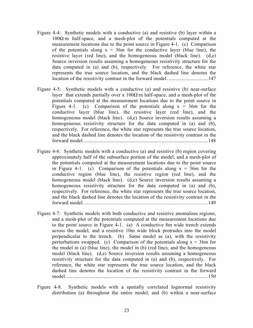
Figure 4-4: Synthetic models with a conductive (a) and resistive (b) layer within a 100Ω·m half-space, and a mesh-plot of the potentials computed at the measurement locations due to the point source in Figure 4-1. (c) Comparison of the potentials along x = 36m for the conductive layer (blue line), the resistive layer (red line), and the homogeneous model (black line). (d,e) Source inversion results assuming a homogeneous resistivity structure for the data computed in (a) and (b), respectively. For reference, the white star represents the true source location, and the black dashed line denotes the location of the resistivity contrast in the forward model. ..............................147

Figure 4-5: Synthetic models with a conductive (a) and resistive (b) near-surface layer that extends partially over a 100Ω·m half-space, and a mesh-plot of the potentials computed at the measurement locations due to the point source in Figure 4-1. (c) Comparison of the potentials along x = 36m for the conductive layer (blue line), the resistive layer (red line), and the homogeneous model (black line). (d,e) Source inversion results assuming a homogeneous resistivity structure for the data computed in (a) and (b), respectively. For reference, the white star represents the true source location, and the black dashed line denotes the location of the resistivity contrast in the forward model...............................................................................................148

Figure 4-6: Synthetic models with a conductive (a) and resistive (b) region covering approximately half of the subsurface portion of the model, and a mesh-plot of the potentials computed at the measurement locations due to the point source in Figure 4-1. (c) Comparison of the potentials along x = 36m for the conductive region (blue line), the resistive region (red line), and the homogeneous model (black line). (d,e) Source inversion results assuming a homogeneous resistivity structure for the data computed in (a) and (b), respectively. For reference, the white star represents the true source location, and the black dashed line denotes the location of the resistivity contrast in the forward model...............................................................................................149

Figure 4-7: Synthetic models with both conductive and resistive anomalous regions, and a mesh-plot of the potentials computed at the measurement locations due to the point source in Figure 4-1. (a) A conductive 8m wide trench extends across the model, and a resistive 10m wide block protrudes into the model perpendicular to the trench. (b) Same model as (a), with the resistivity perturbations swapped. (c) Comparison of the potentials along x = 36m for the model in (a) (blue line), the model in (b) (red line), and the homogeneous model (black line). (d,e) Source inversion results assuming a homogeneous resistivity structure for the data computed in (a) and (b), respectively. For reference, the white star represents the true source location, and the black dashed line denotes the location of the resistivity contrast in the forward model. ...........................................................................................................150

Figure 4-8. Synthetic models with a spatially correlated lognormal resistivity distribution (a) throughout the entire model, and (b) within a near-surface

24

layer, displayed with a mesh-plot of the potentials computed at the measurement locations due to the point source in Figure 4-1. (c) Comparison of the potentials along x = 36m for the model in (a) (blue line), the model in (b) (red line), and the homogeneous model (black line). (d,e) Source inversion results assuming a homogeneous resistivity structure for the data computed in (a) and (b), respectively. For reference, the white star represents the true source location, and the black dashed line denotes the location of the resistivity contrast in the forward model. ......................................................151

Figure 4-9. Smooth 2D (a) and 3D (c) versions of the true resistivity structure in Figure 4-8a used as input to the self-potential source inversion with the simulated data from Figure 4-8a. (b) The source inversion result using the 2D resistivity provides a more compact solution than Figure 4-8d, but the sources are still somewhat mis-located. (d) The use of a smooth 3D resistivity model better estimates the source depth, though there is still some lateral distortion.......................................................................................................................152

Figure 5-1. Comparison of surface self-potential measurements (black line) and PCE concentrations (gray bars) measured in four wells at the A-14 outfall [from Morgan, 2001]. .............................................................................................168

Figure 5-2. Map of the Savannah River Site and surrounding area (site details from Mamatey, [2005]). The A/M area and A-14 outfall are located near the northwest boundary of the site. Black shaded areas are known contaminant plumes...........................................................................................................169

Figure 5-3: Common reaction pathways for the degradation of selected DNAPLs. Those measured at the A-14 outfall are shaded. The left axis shows the reduction potential with respect to ethylene for these reactions [adapted from Vogel et al., 1987]. ........................................................................................170

Figure 5-4: Layout of the surface and borehole self-potential array at the SRS. Seven lines of data are collected on the surface, with station spacing 2-4m. Four 84 foot-deep boreholes surrounding the region of interest each contain seven porous pot electrodes with 3.7m spacing in depth. All measurements are made with respect to a common reference electrode. .............................................171

Figure 5-5: Histogram of SP data measured at the A-14 outfall. The data are smoothly distributed with the exception of a single bad measurement near -100mV. ...172

Figure 5-6: A) 3D self-potential field based on interpolation of surface and borehole data. The reference electrode is located at (-15, 0). B) 3D resistivity model from induced polarization inversion at the A-14 outfall [Briggs et al., 2003].......................................................................................................................173

Figure 5-7: Vertical and horizontal slices of the current source distribution model from the SP inversion. Red areas indicate electrical current sources and blue areas indicate sinks. ......................................................................................174

25

Figure 5-8: Measured versus predicted voltages from the inversion model results. There is a good correlation between data and model, with residuals less than ±5mV. ...........................................................................................................175

Figure 5-9: Isosurfaces of the current source model from the 3D SP inversion at ±12µA. Approximate water table depth is shown in transparent blue, which corresponds well with the broad positive anomaly at the bottom of the model, but is below the electrode array. Further analysis of the sensitivity to the water table is required. ...........................................................................................176

Figure 5-10: Aerial map showing the relative locations of the MIT boreholes and ground truth sampling wells. False Easting and Northing of 15000m and 30000m, respectively, is used for display. .....................................................177

Figure 5-11: Comparison between PCE ground truth concentration data (in log10) and 3D SP inversion model results at the ground truth well locations. SP current source values are scaled based on the best linear fit to the concentration data for all five wells. Error bars represent the standard error of concentration data given by Riha and Rossabi [2003]...................................178

Figure 5-12: This figure shows the general relationship between surface SP data and total PCE concentration in each of the ground truth wells. The highest concentrations are located near larger SP anomalies, and the low concentrations are away from the SP anomaly. This helps to confirm the general relationship between surface SP and contaminated regions. .............179

Figure 6-1: Synthetic example of a gradient SP survey with 10 stations and 13 measurements (based on Cowles [1938]). a) Symbol size and shading represents the ‘true’ station potentials. Gradient data are simulated along four lines (a-d) by calculating potential differences between adjacent stations. b) Interpolated potential field using the 10 stations in a)...................................195

Figure 6-2: Illustration of the l2 inversion results for the data from Figure 6-1 with additional Gaussian noise. The inversion method is able to successfully predict measurements within the expected errors. a) True data that would be measured from the potentials in Figure 6-1a (grey line) with error bars to denote the standard deviation of the added noise, and one realization of noisy measurements (black dots). b) Interpolated potential field found by inverting the noisy measurements. ...............................................................................196

Figure 6-3. Synthetic potential field used to illustrate mis-tie methods. a) Map of the complete potential field with six survey lines annotated. b) True potentials at the survey stations (49 per line, 294 total). c) Synthetic gradient data (potential differences between adjacent stations) for each of the survey lines.......................................................................................................................197

Figure 6-4. Inversion results for the case with Gaussian noise only (σ = 0.96mV). All six lines are displayed sequentially as a function of survey measurement # or

26

station #. a) Comparison of the synthetic noise-free (light grey line) and noisy (grey dots) data with data predicted by the l2 inversion (black dotted line), and the l1 inversion (black dashed line). b) Comparison of the true station potentials (light grey line) with the results from the l2 inversion (black dotted line), and the l1 inversion (black dashed line). ..............................................198

Figure 6-5. Inversion results for the case where 10% of the measurement locations have an unexpectedly large measurement error (σ = 4.8mV) to simulate outliers. All six lines are displayed sequentially as a function of survey measurement # or station #. a) Comparison of the synthetic noise-free (light grey line) and noisy (grey dots) data with data predicted by the l2 inversion (black dotted line), and the l1 inversion (black dashed line). b) Comparison of the true station potentials (light grey line) with the results from the l2 inversion (black dotted line), and the l1 inversion (black dashed line). Black arrows highlight several of the locations most affected by the outliers. ........199

Figure 6-6. Map of Nevis showing the station locations for 19 lines of gradient SP data over an area of approximately 16km2 in the southwest part of the island. The two lines with different shading (labeled a & b) are used for displaying results in subsequent figures. ........................................................................200

Figure 6-7. Inversion results for the field dataset shown along ‘line a’ and ‘line b’ from Figure 6-6. The width of each filled area represents the range of results that are found using different combinations of σ and tar

dφ for the l2 and l1 measures of misfit, while the white dashed line represents the mean result. a) Comparison of the field SP measurements (black dots) with predicted data ( Av ) from the l2 (black area) and l1 (grey area) inversions. b) Range of station potentials predicted along the two transects for the different combinations of σ and tar

dφ for the l2 and l1 measures of misfit....................201

Figure 6-8. Potential field maps calculated using the l2 (a) and l1 (b) inversion methods, interpolated over the entire survey area. In both cases, the mean result from using four different combinations of data weights and target misfit values is illustrated, which corresponds to the white dashed lines in Figure 6-7. c) The difference between the mean l2 and l1 solutions varies in magnitude over the entire survey area, but is almost always positive.............................202

Figure 6-9. Three different versions of the potential field computed using traditional processing methods with lines of data processed in different orders, then interpolated over the entire survey area. Loop closure errors are distributed along new loops as they are completed, but potentials along existing loops are not modified. Because the loops are not independent, this methodology produces inconsistent results.........................................................................203

Figure 7-1: Conceptual schematic of a self-potential secondary source imaging experiment. When fluid is pumped from the well (A), the self-potential

27

response is recorded due to both source types: fluid withdrawal at the well and flow across a boundary. Next, an electric pole source is placed in the screened portion of the well while it is no longer pumping, and the potential field is recorded at the surface (B). Differencing the two datasets leaves only the potential field that is due to induced flow across a boundary. .......................209

Figure A-1.: Schematic of a portion of the 3D transmission network discretization. Adapted from Zhang et al. [1995].................................................................215

Figure A-2: Close-up view of a single impedance branch in the x-z plane. Rx(i,j,k) is determined by the impedance contributions from four resistivity blocks that share the branch, while each Rz comes from a single resistivity block. ........216

Figure C-1: Setup for electroplating the silver mesh. ..............................................227

Figure C-2: Silver mesh electroplated with AgCl. ...................................................228

Figure C-3: Electrode top cap configuration. ..........................................................229

Figure C-4: Porous ceramic cup (from CoorsTek, Inc.)...........................................230

Figure C-5: PVC tube with ceramic cup glued to the end. ......................................231

Figure C-6: Schematic of the porous pot electrode design. .....................................232

Figure C-7: Completed electrodes ...........................................................................233

29

List of Tables

Table 2-1: Parameters used for the synthetic model in Figure 2-4.............................48

Table 3-1: Summary of the combined influence of the minimum support regularization parameters ................................................................................96

Table 3-2: Summary of data and model norms for the inversion results related to the synthetic models in Figure 3-8 and Figure 3-12............................................103

Table 3-3: Summary of data and model norms for the inversion results shown in Figure 3-15 that come from the Bogoslovsky and Ogilvy [1973] dataset.......106

Table 4-1: Summary of data and model norms for the synthetic inversion results based on Figure 4-1.................................................................................................142

Table 6-1: Simulated self-potential dataset for the synthetic example in Figure 6-1.......................................................................................................................185

31

Chapter 1

Introduction

1.1 Motivation and overview of previous research

Self-potentials (SP), sometimes called spontaneous potentials, refer to passively

measured electric potentials that are generated through coupling with some other forc-

ing mechanism; which is often hydraulic, chemical, or thermal. Some of the early ef-

forts to characterize these coupled flow mechanisms in a geophysical context can be

attributed to Marshall and Madden [1959], Sato and Mooney [1960], and Nourbe-

hecht [1963]. Conceptually, it is a very straightforward and versatile technique; elec-

tric signals in an electrically conductive medium (such as the earth) can be detected

remotely from the location of the forcing mechanism. The challenge, to which I at-

tempt to contribute in this thesis, is to be able to make inferences about the underlying

forcing mechanisms from the measured electric signal.

Interest in the self-potential method has been growing for a number of years

(Figure 1-1), with application to various fields within the earth sciences including hy-

drology [Bogoslovsky and Ogilvy, 1973; Fournier, 1989; Birch, 1998; Revil et al.,

2003a; Darnet and Marquis, 2004; Revil et al., 2005; Suski et al., 2006], geothermal

and volcanic systems [Corwin and Hoover, 1979; Fitterman and Corwin, 1982; Ishido

et al., 1983; Morgan et al., 1989; Revil and Pezard, 1998; Aizawa, 2004; Darnet et

al., 2004; Moore et al., 2004], geotechnical and environmental engineering [Corwin,

1990; Perry et al., 1996; Vichabian and Morgan, 2002; Naudet et al., 2003; Naudet et

32

al., 2004; Sheffer et al., 2004], mineral exploration [Sato and Mooney, 1960; Corwin,

1973; Sivenas and Beales, 1982a; Bigalke and Grabner, 1997; Revil et al., 2001;

Heinson et al., 2005], and petrophysics [Ishido and Mizutani, 1981; Morgan et al.,

1989; Revil et al., 1999a; Timm and Moller, 2001; Guichet et al., 2003; Kulessa et al.,

2003; Maineult et al., 2004; Maineult et al., 2005]. In many cases, the self-potential

method has been successfully utilized because of its relative ease-of-use and simplic-

ity in making qualitative interpretations of the measured data. More recent efforts in

this field have continued along these lines, and have also attempted to provide a more

quantitative interpretation.

Consider a simple, but somewhat more intuitive, analogy to this problem: an elec-

tric toaster oven is placed in a room, which is outfitted with an array of temperature

sensors on the walls and ceiling. Given a sufficient number of sensors, one could de-

termine the location of the toaster with reasonable accuracy, though the restriction of

the sensors to the walls and ceiling may lead to some uncertainty. A further degree of

sophistication would involve making some inference about the electric current that is

flowing through the heating coils of the toaster based on the remote measurements of

temperature. While this would likely involve more uncertainty than locating the

toaster, reasonable assumptions about the thermal properties of the toaster materials

and air in the room can at least help to provide an estimate.

The self-potential methods discussed in this thesis attempt to accomplish similar

tasks: (1) to locate the spatial distribution of electric sources in the earth generated by

the coupling mechanism and (2) to characterize the forcing mechanism itself based on

the electric signal. One complication is that the spatial distribution of self-potential

sources can be arbitrary and complicated; the problem is much simpler if one knows a

priori that a point source (like a toaster in a room) is the imaging target.

Throughout this thesis, the forcing mechanism, regardless of its nature, is referred

to as the “source” of the self-potential signal. Thus, the goal of a self-potential survey

is to infer some properties about the source processes from the measured data. This is

in contrast with other geophysical methods such as seismic, radar, or electrical resis-

tivity tomography, which utilize known sources to actively probe structures in the

33

subsurface. Self-potentials are therefore able to provide unique information about

physical and chemical phenomena occurring in the earth that cannot be determined

with other methods.

Compared with controlled-source geophysical methods, self-potential surveys are

relatively simple to undertake due to the minimal and inexpensive equipment that is

required. This simplicity is sometimes an advantage, but can also lead to some diffi-

culty interpreting the data. Given known sources and measured data, physical proper-

ties such as seismic velocity or electric resistivity can be determined. In the self-

potential case, the measured response is a function of both unknown sources and the

unknown resistivity structure. Therefore, there is an inherent ambiguity when inter-

preting the self-potential data when the earth resistivity is unknown. This is some-

what analogous to the earthquake location problem, where passive traveltime meas-

urements are combined with an assumed seismic velocity structure to determine the

earthquake location.

A more direct analogy to the self-potential problem is the electroencephalogram

(EEG), which is a medical imaging technique. The EEG consists of passive meas-

urements of the electric potential field on a person’s scalp, which can vary due to

electrical activity within the brain. The goal of EEG data interpretation is to localize

these sources in the brain, providing useful information about regions that are acti-

vated by some external stimulus or medical condition such as epilepsy [e.g. Michel et

al., 2004, and references within]. While self-potentials and EEG have completely dif-

ferent spatial scales and applications, the underlying problem is the same; an un-

known electrical source within a heterogeneous volume conductor (the earth or a per-

son’s skull) produces a remotely measurable potential field, which is subsequently

used to characterize the source. Therefore, many of the same concepts and data proc-

essing techniques from one problem may provide useful insights for the other.

Various approaches have been developed to interpret self-potential data [e.g. Fit-

terman, 1979a; Fitterman and Corwin, 1982; Fournier, 1989; Patella, 1997; Birch,

1998; Gibert and Pessel, 2001; Revil et al., 2001; Sailhac and Marquis, 2001; Darnet

and Marquis, 2004; Revil et al., 2004; Sheffer et al., 2004; Minsley et al., 2007], and

34

there is a large volume of related work in the medical community [e.g. Pascual-

Marqui et al., 1994; Malmivuo et al., 1997; Marin et al., 1998; Pascual-Marqui,

1999; Michel et al., 2004; Wolters et al., 2004; Wolters et al., 2006]. Some of these

can be termed “forward” methods, where the measured data are replicated by system-

atically varying different source parameters (e.g. source depth, spatial distribution,

intensity, etc.). Alternatively, “inverse” methods utilize the measured data directly to

characterize the source properties. Both approaches can be useful, though this thesis

focuses primarily on the inverse techniques.

Several processing steps for the self-potential problem can be effectively bor-

rowed from somewhat more developed electrical resistivity algorithms [Fitterman,

1979b; Wurmstich, 1995; Shi, 1998]. In the resistivity inverse problem, a limited

number of sources with known intensity and location are utilized, and the recorded

potentials are used to infer the resistivity structure of the earth. In the self-potential

inverse problem, recorded potentials are combined with an assumed resistivity struc-

ture to recover an unknown distribution of sources. Both of these methods, however,

rely heavily on efficient methods of computing the potential field due to multiple

known source distributions and resistivity structures.

As with all geophysical techniques, data errors degrade our ability to interpret the

measured signal. Common sources of self-potential measurement error can be associ-

ated with the degradation or drift of the measuring electrodes, poor contact between

the electrode and soil, and cultural noise. Numerous authors have investigated elec-

trode designs that reduce measurement errors and are stable over long periods of time

[Corwin, 1973; Perrier et al., 1997; Clerc et al., 1998; Petiau, 2000]. Measurement

errors on the order of several (~5) millivolts should be expected with modern survey-

ing equipment, and this can be significantly reduced by installing the electrodes

(semi) permanently [Perrier et al., 1997; Perrier and Pant, 2005]. The influence of

cultural noise (e.g. power lines, cathodic protection, grounding systems) can be sig-

nificant [Corwin, 1990], and should be accounted for when surveys are conducted

near developed areas. Of course, the level of noise should be considered with respect

35

to the magnitude of the measured signal; large anomalies that register hundreds of

millivolts should not be significantly influenced by relatively small errors.

The self-potential source inversion problem is highly non-unique; there are many

possible distributions of sources that fit the data equally. This dilemma is common to

nearly all geophysical inverse problems, and is exacerbated by the fact that measure-

ment locations are often restricted to relatively few locations on the earth’s surface.

Additionally, the self-potential response depends on the resistivity structure of the

earth, which is never perfectly known. One approach to reducing the non-uniqueness

of the problem is to introduce constraints in the inverse problem based on prior as-

sumptions about the properties of the source model. I address these issues in this the-

sis by: (1) utilizing non-traditional inversion constraints that are appropriate for self-

potential sources, (2) incorporating available resistivity information into the inversion

algorithm, and (3) understanding the effects of uncertainty in the resistivity structure

on the source inversion results.

1.2 Outline of thesis

The main goal of this thesis is to develop processing algorithms that aid in the acqui-

sition and interpretation of self-potential data. My approach is general in the sense

that this methodology can be applied to SP data generated by any source mechanism.

This is accomplished by separating the problem into two steps. The first step, which

is the main focus of this thesis, involves the inversion of measured SP data to recover

the spatial distribution of electrical sources that generate the signal. In some cases,

simply understanding the distribution of sources in the earth can provide useful in-

sights into a problem. Next, the distribution of source amplitudes can be interpreted

in terms of the physical relationship that describes the coupling between a primary

forcing process and the electrical response.

Chapter 2 provides background information regarding the origin of self-potential

signals generated by hydraulic and chemical forcing mechanisms, and several simple

examples are presented to give some insight into the general behavior of the coupled

36

phenomena. A brief description of the possible types of self-potential sources, in the

context discussed by Sill [1983] and Wurmstich [1995], is also presented. Finally, a

“realistic” synthetic example based on an aquifer storage and recovery (ASR) experi-

ment is presented to highlight several aspects of self-potential sources. More than to

present new information, this chapter seeks to clarify several frequent misconceptions

regarding self-potential sources.

Chapter 3 describes the self-potential source inversion methodology, which is a

central component of this thesis. The result of the source inversion is a distribution of

electric current sources that support the measured data. Self-potential source inver-

sion is a linear problem, though the use of a non-linear model regularization scheme

that promotes spatially compact sources (rather than traditional smoothness con-

straints) requires an iterative solution method. Available resistivity information can

be incorporated into the Green’s functions for the inversion, which are also utilized to

implement sensitivity scaling. Synthetic examples illustrate the utility of this ap-

proach, and provide some insight into how resistivity uncertainty affects the inversion

results. Field data from a previously published self-potential survey [Bogoslovsky

and Ogilvy, 1973] in the vicinity of a water well are subsequently inverted. This

dataset is chosen because it has been the focus of several other self-potential studies

[Darnet et al., 2003; Revil et al., 2003a]. The bulk of this chapter is published as:

• Minsley, B.J., J. Sogade, and F.D. Morgan (2007), Three-dimensional source

inversion of self-potential data, Journal of Geophysical Research, 112,

B02202, doi:10.1029/2006JB004262.

Chapter 4 discusses in detail the effects of resistivity uncertainty on the self-

potential source inversion, and is accomplished in two phases. First, the problem is

approached by deriving the effect of resistivity uncertainty on the self-potential re-

sponse for a known source using a Taylor expansion. This provides useful insights

into the situations where resistivity uncertainty has the greatest effect on the source

inversion. This derivation is very general, and does not presume any particular model

geometry, acquisition array, or source structure. The second part of this chapter pre-

sents several synthetic examples where self-potential data are simulated using a sim-

37

ple point source and known resistivity structure. These data are then inverted using

the methods discussed in Chapter 3, with an incorrect (homogeneous) resistivity

structure. Errors in the recovered sources provide useful insights into the effect of

various forms of resistivity uncertainty. The latter portion of this chapter was pre-

sented as a poster at the Fall 2006 AGU meeting in San Francisco, and received the

outstanding student paper award for the Near-Surface section:

• Minsley, B. and F.D. Morgan (2006), Quantifying the effects of unknown re-

sistivity structure on self-potential inversion, EOS Trans. AGU, 87(52), Fall

Meet. Suppl., Abstract NS31A-1562.

The entire chapter will be submitted as a manuscript with the same title to the Journal

of Geophysical Research, with authors Minsley, B., W. Rodi, and F.D. Morgan.

Chapter 5 is a case study where the inversion procedure is applied to self-potential

data collected at the Savannah River Site in South Carolina. This is a relatively

unique self-potential dataset, as it consists of both surface and borehole measurements

surrounding a contaminated site. These data were collected by me and others from

the Earth Resources Lab during a field campaign in 2003, in conjunction with a 3D

induced polarization survey at the same site. Self-potentials associated with the deg-

radation of contaminants in the environment is an active area of research, and still re-

quires further work to fully understand the electrochemical mechanisms that generate

the signal. This chapter is recently published as:

• Minsley, B., J. Sogade, and F.D. Morgan (2007), Three-dimensional self poten-

tial inversion for subsurface DNAPL contaminant detection at the Savannah

River Site, South Carolina, Water Resources Research, 43, W04429,

doi:10.1029/2005WR003996.

Chapter 6 presents a pre-processing method for self-potential datasets collected

with complicated survey geometries. This technique was developed as a result of a

large self-potential survey carried out in Nevis, West Indies during a geothermal ex-

ploration campaign in which I participated in 2004. Traditionally, survey lines are

collected such that they form closed loops; data errors are accounted for at the closure

points, and multiple survey lines are connected at their intersection points. When

38

many survey lines form multiple interconnected loops, however, a unique potential

map cannot be determined by processing survey lines sequentially using the tradi-

tional approach. This chapter presents a methodology for processing all survey lines

simultaneously using a least-squares algorithm. A unique potential map is generated

that minimizes the loop closure errors over the entire survey using either an l2 or l1

measure of misfit. In the presence of data outliers, which are common to many self-

potential surveys, the l1 measure tends to produce superior results. This chapter is in

preparation for Geophysical Prospecting:

• Minsley, B., D. Coles, Y. Vichabian, and F.D. Morgan, Accounting for mis-ties

on self-potential surveys with complicated acquisition geometries, Geophysi-

cal Prospecting, in preparation.

39

Figure 1-1: Number of publications per year with topic “self-potential” based on a search of the Thomson ISI Web of Knowledge database. N.B: related terms such as “spontaneous potential” or “electrokinetic” were not searched due to a large number of hits from non-geophysical applications.

41

Chapter 2

Self-potential background

2.1 Overview of the origin of self-potentials

Self-potentials are the result of coupling between electric and non-electric flows and

forces in the earth. On the macroscopic scale, coupled transport phenomena are typi-

cally discussed in the context of non-equilibrium thermodynamics [e.g. de Groot,

1951], and it is assumed that fluxes are linearly related to driving forces. This results

in a linear system of coupled equations (2.1), where the ijL are phenomenological

coupling coefficients that link the forces ( iX ) to fluxes ( iq ).

11 12 13 141 1

21 22 23 242 2

31 32 33 343 3

41 42 43 444 4

L L L Lq XL L L Lq XL L L Lq XL L L Lq X

⎡ ⎤⎡ ⎤ ⎡ ⎤⎢ ⎥⎢ ⎥ ⎢ ⎥⎢ ⎥⎢ ⎥ ⎢ ⎥=⎢ ⎥⎢ ⎥ ⎢ ⎥⎢ ⎥⎢ ⎥ ⎢ ⎥

⎣ ⎦ ⎣ ⎦⎣ ⎦

(2.1)

Onsager [1931] showed that, for small flows, the matrix of coupling coefficients is

symmetric (i.e. ij jiL L= ). The system of coupled phenomena is often referred to as

Onsager’s reciprocal relations, for which he was awarded the Nobel Prize in Chemis-

try in 1968.

Typical forces and their conjugated fluxes are: electric potential gradients and

electric current density (Ohm’s Law), hydraulic gradients and fluid flux (Darcy’s

Law), chemical gradients and solute flux (Fick’s Law), and thermal gradients and heat

42

flow (Fourier’s Law). Because of the coupling described by equation (2.1), it is also

possible to have contributions to any of the fluxes from any other non-conjugated

forcing, i.e.

i ij jj

q L X= ∑ . (2.2)

All sixteen possible phenomena are summarized in Figure 2-1.

The total electric current density 1j q= [A·m-2] in the earth can have a contribu-

tion from all four forces, i.e.

( ) ( ) ( ) ( ) ( )c k d tj j j j j= + + +x x x x x . (2.3)

jk is the streaming current due to hydraulic forcing, jd is the diffusion current due to

chemical forcing, jt is the current due to thermal forcing, and jc is the familiar conduc-

tion current

( ) ( ) ( )cj Eσ=x x x , (2.4)

where ( )σ x [S·m-1] represents the earth conductivity structure and ( )E x is the elec-

tric field.

The self-potential problem, by definition, is concerned only with currents that

vary on the time scale of the forcing mechanism, which is generally very slow for

processes in the earth. Therefore, the quasi-static from of Maxwell’s equations can be

applied. By neglecting the magnetic induction in Faraday’s Law,

0BEt

∂∇× = − ≅

∂ (2.5)

the electric field can be written as the negative gradient of the scalar electric potential,

( )ϕ x [V].

( ) ( )E ϕ= −∇x x (2.6)

Taking the divergence of Ampère’s Law (2.7)

( ) 0EH jt

ε∂⎛ ⎞∇ ⋅ ∇× = ∇ ⋅ + =⎜ ⎟∂⎝ ⎠, (2.7)

and substituting Gauss’ Law (2.8)

43

( ) qEε ρ∇ ⋅ = , (2.8)

yields the equation for the conservation of charge

qjt

ρ∂∇ ⋅ = −

∂. (2.9)

In equations (2.7) and (2.8), ε is the electric permittivity [F·m-1], ρq is the charge den-

sity [C·m-3], and j is the total current density from equation (2.3). For the quasi-static

case, the time derivative of the charge density is neglected, resulting in the familiar

equation for the conservation of current.

0j∇ ⋅ = (2.10)

Self-potentials are the measurable electric potentials associated with a conduction

current ( cj ) that is due to coupling with one or more forcing phenomena. That is, the

electric potential is the response to some other forcing mechanism. Substituting equa-

tion (2.3) into equation (2.10), and separating the forcing from the electrical response

gives

( ) ( ) ( )( )sj sσ ϕ−∇ ⋅ ∇ = ∇ ⋅ =x x x x . (2.11)

Thus the source term ( )s x [A·m-3] equals the divergence of the sum of the current

densities due to the forcing mechanism(s), i.e.

11

s k d t j jj

j j j j L X≠

= + + = ∑ . (2.12)

The coupling coefficients, ijL , found in the source term clearly play an important

role in determining the self-potential response. A significant amount of research has

therefore gone into understanding the coupling coefficients for various forcing

mechanisms [e.g. Ishido and Mizutani, 1981; Morgan et al., 1989; Pride, 1994; Revil

et al., 1999a; Reppert, 2000]. While the coupling coefficient is not a focus of this

thesis, a brief review of the coupling for electrokinetic and electrochemical processes

is presented in the following two sections as the concepts are relevant to subsequent

discussions.

44

2.1.1 Streaming potentials and the Helmholtz-Smoluchowski equation

Streaming potentials result from the coupling between fluid flow and electric conduc-

tion in porous media, a phenomenon sometimes called the electrokinetic effect

[Overbeek, 1952]. The buildup of an excess charge in the vicinity of fluid-solid inter-

faces is described by the physics of the electric double layer. [e.g Guéguen and Palci-

auskas, 1994; Bockris and Reddy, 2000] (Figure 2-2). For most earth materials, the

solid surface exhibits a negative charge, resulting in an excess of positive counterions

in the fluid. Near the fluid-solid interface, charges are tightly bound within the inner

and outer Helmholtz layers, also called the Stern layer, and are immobile under a hy-

draulic gradient. Beyond this distance (typically on the order of several Angstroms),

the density of excess charge decays in a diffuse cloud. Drag of the excess charge un-

der a hydraulic gradient results in a streaming current density within the fluid ( kj in

equation (2.3)).

k qj uρ= (2.13)

qρ represents the charge density [C·m-3] and u is the fluid velocity [m·s-1].

Consider fluid flow through a cylindrically-shaped pore (or capillary) under a

static pressure gradient (Figure 2-3). The fluid velocity is described by Poiseuille’s

Law

( )2 2( )4

Pu r a rlη

∆= − , (2.14)

where P∆ is the applied pressure drop across the ends of the pore [Pa], η is the fluid

viscosity [Pa·s], l is the pore length [m], a is the pore radius [m], and r is the radial

coordinate within the pore [m]. The charge density is also a function of distance from

the pore wall, and is governed by Gauss’ Law (in radial coordinates)

1 ( ) qd d rrr dr dr

ρψε

−= , (2.15)

45

where ( )rψ describes the potential [V] with distance from the pore wall due to the

excess charge. The zeta-potential, ζ [V], is defined as the potential at the distance

from the pore wall where the charge can be dragged with the fluid ( r s a= ≈ ), as it is

tightly bound within the double layer for s r a< < (Figure 2-2).

The divergence theorem can be used to convert the integral of equation (2.11) over

the volume of the cylinder into a surface integral of the total current density

( ) ( )( ) ( ) ( ) ( ) 0c k c kV V

j j dV j j dS∂

∇ ⋅ + = ⋅ + =∫ ∫x x n x x . (2.16)

The total current, I [A], flowing across a surface is defined by the integral of the cur-

rent density over the surface

( )S

I j dS= ⋅∫n x . (2.17)

At equilibrium, equation (2.16) implies that the total current through a surface is zero,

and the streaming current is balanced by the conduction current.

( ) ( )c c k kS S

j dS I I j dS− ⋅ = − = = ⋅∫ ∫n x n x (2.18)

It is important to note that the total current through a surface equals zero, but the cur-

rent at any given point in the system may be non-zero. This can be a source of some

confusion in self-potential interpretation, and will be discussed in more detail later.

Equations (2.13) through (2.15) are combined in equation (2.18) to compute kI

( )2 2

0

( )2

s

kP d d rI dr r a r

l dr drεπ ψ

η− ∆

= −∫ . (2.19)

Integrating by parts gives

( ) ( )2 2

0 0

( ) ( )22

s s

kP d r d rI a r r dr r r

l dr drεπ ψ ψ

η⎡ ⎤− ∆

= − − −⎢ ⎥⎢ ⎥⎣ ⎦

∫ , (2.20)

where the first term in brackets evaluates to zero under the approximation that a s≈ .

Integrating by parts a second time gives

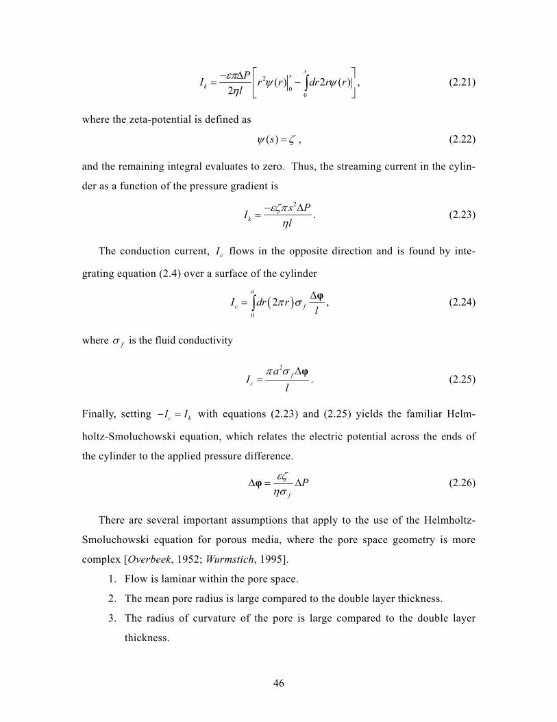
46

2

00

( ) 2 ( )2

ss

kPI r r dr r r

lεπ ψ ψ

η⎡ ⎤− ∆

= −⎢ ⎥⎣ ⎦

∫ , (2.21)

where the zeta-potential is defined as

( )sψ ζ= , (2.22)

and the remaining integral evaluates to zero. Thus, the streaming current in the cylin-

der as a function of the pressure gradient is

2

ks PIl

εζπη

− ∆= . (2.23)

The conduction current, cI flows in the opposite direction and is found by inte-

grating equation (2.4) over a surface of the cylinder

( )0

2a

c fI dr rl

π σ ∆= ∫

φ , (2.24)

where fσ is the fluid conductivity

2

fc

aI

lπ σ ∆

=φ

. (2.25)

Finally, setting c kI I− = with equations (2.23) and (2.25) yields the familiar Helm-

holtz-Smoluchowski equation, which relates the electric potential across the ends of

the cylinder to the applied pressure difference.

f

Pεζησ

∆ = ∆φ (2.26)

There are several important assumptions that apply to the use of the Helmholtz-

Smoluchowski equation for porous media, where the pore space geometry is more

complex [Overbeek, 1952; Wurmstich, 1995].

1. Flow is laminar within the pore space.

2. The mean pore radius is large compared to the double layer thickness.

3. The radius of curvature of the pore is large compared to the double layer

thickness.

47

4. The effects of surface conduction can be neglected, though there are several

modifications to equation (2.26) that take this into account [Ishido and Mi-

zutani, 1981; Morgan et al., 1989; Revil et al., 1999b].

The term that relates the electric potential difference to the applied pressure dif-

ference across a sample is often called the voltage coupling coefficient [V·Pa-1],

f

C εζησ

= . (2.27)

The voltage coupling coefficient is useful because it is readily measurable in the labo-

ratory, and is frequently reported in the literature. Modeling self-potentials according

to equation (2.11), however, requires knowledge of the current coupling coefficient, L

[A·Pa-1·m-1]. The voltage and current coupling coefficients are related by the bulk

conductivity of the sample,

rL Cσ= − . (2.28)

The ratio of the bulk conductivity to fluid conductivity is often referred to as the for-

mation factor, F, and equation (2.28) can be written as

LFεζ

η−

= . (2.29)

Note that the Helmholtz-Smoluchowski equation (2.26) is the result that follows

from the physics defined in equation (2.11), but should not be interpreted as a general

rule that holds everywhere. That is, self-potentials can be measured between two

points on the earth surface, but this does not necessarily imply that there is a hydrau-

lic gradient between the measurement locations. For example, consider the situation

where fluid flow occurs due to a hydraulic gradient in a subsurface confined aquifer.

Self-potential measurements can be made between two electrodes on the earth sur-

face, even though the fluid flow occurs only at depth.

In general, the streaming and conduction currents can occupy different domains

and have different boundary conditions. This is related to the earlier comment that,

while the total current in a system equals zero, it is not necessarily zero at every point

within the system. Additionally, when the streaming and conduction currents occupy

48

different domains, the maximum potential drop in the system may be lower than that

predicted by equation (2.26). This can occur when a layer with relatively high con-

ductivity effectively short circuits the system, and the conduction current can balance

the streaming current with a smaller potential drop.

These concepts are illustrated in several simple synthetic examples where fluid

flow in a porous sample is modeled by Darcy’s Law. An applied pressure gradient

produces the streaming current and coupled electric potentials. The two-way coupled

equations are therefore

rj L Pσ ϕ= − ∇ − ∇ (2.30)

kq L Pϕη

= − ∇ − ∇ , (2.31)

where k is the hydraulic permeability [m2]. The first term in equation (2.31) is typi-

cally dropped because the gradient of the generated streaming potential is typically

small, and results in negligible additional flow compared with that due to the hydrau-

lic gradient. The following examples are therefore only one-way coupled.

Figure 2-4a shows the model geometry for the first example, which is a 2D homo-

geneous sample with dimensions 10cm x 2.5cm, though these concepts can easily be

applied to field scales as well. The input parameters for this example are summarized

in the center column of Table 2-1. The hydraulic boundary conditions consist of an

applied pressure difference of 9800Pa (1m of head) between the ends of the sample,

and no-flow conditions along the top and bottom of the sample. For the electric prob-

lem, a no-flow boundary condition is specified on all four sides, and the reference po-

tential location is at the bottom-left corner.

Table 2-1: Parameters used for the synthetic model in Figure 2-4. Model A Model B

rσ [S·m-1] 0.01 0.01

(2)rσ [S·m-1] N/A 0.01, 0.1, 0.001

L [A·Pa-1·m-1] 91.5 10x − 91.5 10x −

49

Model A Model B

k [m2] 121 10x − 121 10x −

η [Pa·s] 0.001 0.001

P∆ [Pa] 9800 9800

The finite element software package, COMSOL MultiphysicsTM 3.2, provides a

versatile way to solve coupled multiphysics problems such as this one. Equations

(2.30) and (2.31) are solved under the condition 0j∇ ⋅ = and 0q∇ ⋅ = , which is

equivalent to solving equation (2.11) with the source current determined by the speci-

fied coupling coefficient and pressure gradients determined from Darcy’s Law.

Figure 2-5 illustrates the solution to this problem, where the color image depicts

the electric potentials; the contours are lines of constant pressure; and the arrows rep-

resent different portions of the electric current density. The arrows depict the source

current (2nd term in equation (2.30)) in Figure 2-5a, the conduction current ( cj ) in

Figure 2-5b, and the total current ( s cj j+ ) in Figure 2-5c. For this simple example

where the hydraulic and electric domains are the same, the total current is zero at each

point in the model.

A 1cm layer is added to this geometry for the next example, as shown in Figure

2-4b. In this case, however, fluid flow is restricted to the original lower domain

rather than the entire sample. This is accomplished by solving the hydraulic problem

only in the lower portion of the model, where the same pressure difference is applied

between the lower ends of the sample, and the no-flow boundary condition for the

fluid is now at the interface between layers. The electric problem is solved over the

entire domain, where the bulk conductivity can be specified separately for each layer.

A no-flow condition is still specified for the electric current density on the outside

edges of the model, and continuity of the total current density ( 1 2( ) 0j j⋅ − =n ) is

given at the interface between layers.

In the earth, this might correspond to the situation where there is a hydraulic gra-

dient within a confined aquifer at depth. Fluid flow is restricted to the aquifer, but the

50

entire earth structure above the aquifer is typically at least partially saturated and

therefore electrically conductive. The following three examples maintain the same

parameters as the first example, but the conductivity of the upper layer is varied (see

Table 2-1).

In Figure 2-6, the upper layer has the same bulk conductivity as the lower layer,

i.e. -1(2) 0.01 S mr rσ σ= = ⋅ . Fluid flow, and therefore the source current ( sj ) de-

picted by arrows in Figure 2-6a, is confined to the lower layer because of the imposed

hydraulic boundary conditions. This source current drives a conduction current,

shown by the arrows in Figure 2-6b, throughout the entire domain due to the conser-

vation of total current required by equation (2.11). The total current density in Figure

2-6c is non-zero throughout the model, in contrast with the previous example in

Figure 2-5 where the total current was zero at every point. For the two-layer case in

Figure 2-6, the total current density passing through any vertical cross-section of the

model equals zero, which is a result of satisfying equation (2.16).

Figure 2-7 and Figure 2-8 shows the same series of images for the cases where the

bulk electric conductivity of the upper layer equals 0.001 S·m-1 and 0.1 S·m-1, respec-

tively. All other parameters for these examples remain unchanged, resulting in the

same source current (Figure 2-7a and Figure 2-8a). Because of the differences in the

bulk conductivity of the upper layer, however, the conduction current is partitioned

between the two layers depending on the ratio of their conductivities (Figure 2-6b,

Figure 2-7b, Figure 2-8b). Proportionally more current flows in the layer with the

higher conductivity, though the total current through any vertical cross-section is still

zero.

In Figure 2-7b, very little of the conduction current flows in the upper layer where

the conductivity is smaller than that of the lower layer. Note that the actual magni-

tude of the total current density in the upper layer of Figure 2-7c is the same as the

(relatively small) conduction current shown in the upper layer of Figure 2-7b, but has

been scaled relative to the maximum value. In the limiting case where the upper layer

conductivity becomes very small, virtually all of the conduction current flows in the

lower layer, resulting in zero total current at each location as in Figure 2-5c.

51

A significant amount of the conduction current flows in the upper layer in Figure

2-8b due to the relatively high electric conductivity compared with the lower layer.

Again, this results in a non-zero total current density at any particular location (Figure

2-8c), though the total current density passing through any vertical cross-section is

still zero.

Another feature that becomes apparent in Figure 2-8 is the short-circuiting effect

mentioned earlier, where the maximum electric potential drop for a given applied hy-

draulic pressure difference depends on the upper-to-lower layer bulk conductivity ra-

tio. This is illustrated in Figure 2-9, which shows the maximum electric potential dif-

ference across the model for a range of upper-to-lower layer bulk conductivity values,

where all other modeling parameters remain fixed. As this ratio becomes very small,

the maximum electric potential difference asymptotes to the value predicted by the

Helmholtz-Smoluchowski equation (2.26). For large values of upper-to-lower layer

conductivity ratio, the maximum electric potential difference is approximately one-

third of the value predicted by equation (2.26). This reduction in the potential differ-

ence is due to the decrease in effective resistance of the model, though the magnitude

of this effect depends on the particular details of the model geometry.

2.1.2 Diffusion potentials and the Nernst equation

Another common mechanism for generating self-potentials involves the coupling be-

tween chemical gradients and electric current density. The molar flux [mol·m-2·s-1] of

the ith ionic species (i.e. q+ or q− in a 1:1 electrolyte) due to a concentration gradient

is described by Fick’s Law,

i i iq D c= − ∇ , (2.32)

where D [m2·s-1] is the diffusion coefficient and c [mol·m-3] is the concentration. Ac-

cording to the Einstein relation, the diffusion coefficient can be written in terms of the

ionic mobility, u [m2·V-1·s-1]; Boltzmann’s constant, k [ 231.38 10x − J·K-1]; temperature,

T [K]; and total ionic charge, ez [C], where e is the elementary charge 191.6 10x − C

[Bockris and Reddy, 1998].

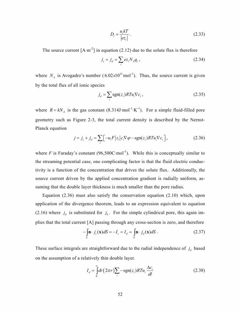
52

ii

i

u kTDez

= . (2.33)

The source current [A·m-2] in equation (2.12) due to the solute flux is therefore

s d i A ii

j j ez N q= = ∑ , (2.34)

where AN is Avogadro’s number ( 236.02 10x mol-1). Thus, the source current is given

by the total flux of all ionic species

sgn( )d i i ii

j z RTu c= ∇∑ , (2.35)

where AR kN= is the gas constant (8.314J·mol-1·K-1). For a simple fluid-filled pore

geometry such as Figure 2-3, the total current density is described by the Nernst-

Planck equation

sgn( )c d i i i i i ii

j j j u F z c z RTu cϕ= + = ⎡− ∇ − ∇ ⎤⎣ ⎦∑ , (2.36)

where F is Faraday’s constant (96,500C·mol-1). While this is conceptually similar to

the streaming potential case, one complicating factor is that the fluid electric conduc-

tivity is a function of the concentration that drives the solute flux. Additionally, the

source current driven by the applied concentration gradient is radially uniform, as-

suming that the double layer thickness is much smaller than the pore radius.

Equation (2.36) must also satisfy the conservation equation (2.10) which, upon

application of the divergence theorem, leads to an expression equivalent to equation

(2.16) where dj is substituted for kj . For the simple cylindrical pore, this again im-

plies that the total current [A] passing through any cross-section is zero, and therefore

( ) ( )c c d dS S

j dS I I j dS− ⋅ = − = = ⋅∫ ∫n x n x . (2.37)

These surface integrals are straightforward due to the radial independence of dj based

on the assumption of a relatively thin double layer.

( )0

2 sgn( )a

id i i

i

cI dr r z RTudl

π ∆= −∑∫ (2.38)

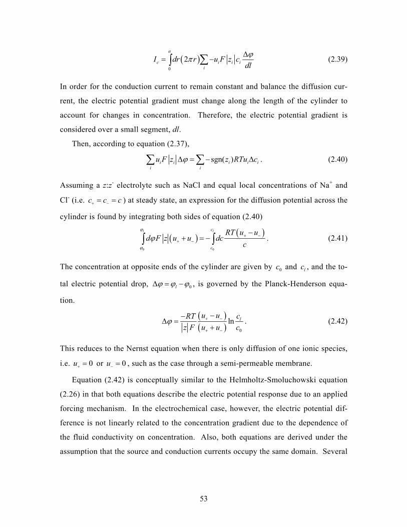
53

( )0

2a

c i i ii

I dr r u F z cdlϕπ ∆

= −∑∫ (2.39)

In order for the conduction current to remain constant and balance the diffusion cur-

rent, the electric potential gradient must change along the length of the cylinder to

account for changes in concentration. Therefore, the electric potential gradient is

considered over a small segment, dl.

Then, according to equation (2.37),

sgn( )i i i i ii i

u F z z RTu cϕ∆ = − ∆∑ ∑ . (2.40)

Assuming a z:z- electrolyte such as NaCl and equal local concentrations of Na+ and

Cl- (i.e. c c c+ −= = ) at steady state, an expression for the diffusion potential across the

cylinder is found by integrating both sides of equation (2.40)

( ) ( )0 0

l lc

c

RT u ud F z u u dc

c

ϕ

ϕ

ϕ + −+ −

−+ = −∫ ∫ . (2.41)

The concentration at opposite ends of the cylinder are given by 0c and lc , and the to-

tal electric potential drop, 0lϕ ϕ ϕ∆ = − , is governed by the Planck-Henderson equa-

tion.

( )( ) 0

ln lu u cRTz F u u c

ϕ + −

+ −

−−∆ =

+. (2.42)

This reduces to the Nernst equation when there is only diffusion of one ionic species,

i.e. 0u+ = or 0u− = , such as the case through a semi-permeable membrane.

Equation (2.42) is conceptually similar to the Helmholtz-Smoluchowski equation

(2.26) in that both equations describe the electric potential response due to an applied

forcing mechanism. In the electrochemical case, however, the electric potential dif-

ference is not linearly related to the concentration gradient due to the dependence of

the fluid conductivity on concentration. Also, both equations are derived under the

assumption that the source and conduction currents occupy the same domain. Several

54

examples in section 2.1.1 show that equation (2.26) does not hold when this assump-

tion is not valid, and a similar argument can be made for equation (2.42).

2.1.3 Electrochemical potentials associated with redox proc-esses

A significant amount of self-potential literature is related to redox phenomena in the

earth, particularly in the context of mineral exploration. In one of the earliest re-

ported observations of naturally occurring electric gradients related to ore bodies, Fox

[1830, p. 400] hypothesized that

“.. it seems likely that electro-magnetism may become useful to the

practical miner in determining with some degree of probability at least,

the relative quantity of ore in veins, and the directions in which it most

abounds.”

While this prediction has certainly proven true in modern exploration geophysics, Fox

[1830] attributed his observations to a thermal, rather than electrochemical, mecha-

nism. This is not entirely surprising, as his work came only thirty years after Gal-

vani’s invention of the Voltaic pile, and preceded both Kirchoff’s circuit laws (1845)

and Maxwell’s equations (1861).

Large self-potential anomalies, sometimes on the order of hundreds of millivolts,

have successfully delineated areas with economically relevant mineral resources. De-

spite this accomplishment, the electrochemical mechanisms that generate these sig-

nals remain somewhat a topic of confusion and controversy. This is partly due to the

interpretation of self-potentials in the earth based on the Galvanic cell (Figure 2-10a)

in the context of equilibrium thermodynamics, which is discussed here in more detail.

Most of the contemporary literature in this field is based on the work of Sato and

Mooney [1960], who attribute the measurable self-potentials to the ohmic potential

drop in the rock and soil surrounding an ore body that is part of an electrochemical

cell. In their model, the ore does not participate in the redox reactions, but serves as

an electronic conductor that spans a gradient in the subsurface redox conditions

(Figure 2-11). Sato and Mooney [1960] suggest the case where the ore straddles the

55

water table, resulting in a spontaneous electrochemical cell where electronation reac-

tions take place in the upper portion (cathode) and de-electronation occurs at depth

(anode). This is similar to the case illustrated in Figure 2-10b, which is analogous to

the corrosion of an iron pipe that spans regions of different redox conditions in the

earth [Bockris and Reddy, 1970; Corwin, 1990].

A number of authors have discussed electrochemical mechanisms as the driving

force for self-potential signals related to buried ores in this context [Nourbehecht,

1963; Sivenas and Beales, 1982b; Sivenas and Beales, 1982a; Kilty, 1984; Bigalke

and Grabner, 1997]. An important distinction that is sometimes overlooked is the

fact that the electrochemical systems relevant to the self-potential problem are not in

equilibrium. If the system were in equilibrium, no current would flow through the

earth external to the ore body and there would therefore be no ohmic potential drop

(and hence no measurable self-potential).

In the Galvanic cell (Figure 2-10a), equilibrium conditions exist when either the

load or electrolyte resistances ( lR or eR ) become very large such that no current can

flow. In this open-circuit case, the cell potential measured between the two electrodes

is the equilibrium potential as defined by the Nernst equation, and can be found in a

table of standard electrode potentials. Note, however, that this potential can only be

measured by placing the measurement system in direct contact with the zinc and cop-

per electrodes.

Consider the following analogy to the streaming potentials discussed earlier in

Figure 2-5 through Figure 2-8. If a hydraulic pressure difference is applied between

the two ends of the sample, but a valve is closed that prohibits fluid flow through the

sample, there is no self-potential signal. The only way to infer something about the

hydraulic pressure difference is to directly measure the pressure outside the sample.

When lR and eR are finite, however, the electrochemical reactions at the anode

and cathode drive a current through the system; electronic from the electrodes through

the load resistance, and ionic in the electrolyte. Due to the flow of current in this

non-equilibrium state, the potential difference across the load drops from the equilib-

rium potential. Continuing the analogy with the hydraulic example, this is equivalent

56

to the situation where the potential difference across the sample is lower than that

predicted by the Helmholtz-Smoluchowski due to the conduction current outside the

domain of the convection current (Figure 2-6 through Figure 2-9). This phenomenon

is observed when a load is connected to a battery, and the measurable potential be-

tween the terminals is reduced.

The current in the system is determined by the various resistances. There are two

more “resistances” in Figure 2-10 ( interfaceR ), which are associated with the metal-

electrolyte interface at the two electrodes. These are not resistances in the traditional

sense, but are described by the Butler-Volmer equation (2.43) which relates the cur-

rent density crossing the electrode-electrolyte interface to the potential across the in-

terface [e.g. Bockris and Reddy, 1970; Bard and Faulkner, 1980].

( )2 20

nF RT nF RTj j e eη η−= − (2.43)

The importance of this equation is significant because it describes the current den-

sity, j, in non-equilibrium systems. The potential that develops across the interface

due to current flow is the overpotential (η [V]), which is defined as the departure of

the potential drop across lR and eR ( l eV V∆ + ∆ ) from the equilibrium potential ( 0V∆ ).

( )0 e lV V Vη = ∆ − ∆ + ∆ . (2.44)

Here, η represents the overpotential through both the anode and cathode, i.e.

1 2η η η= − , but the net effect is additive since they are of opposite signs. 0j is the

equilibrium exchange current density, and is dependent on the kinetics of the interfa-

cial system as well as the electrode and electrolyte properties [Bockris and Reddy,

1970]. F is Faraday’s constant, R is the gas constant, T is the temperature, and n is

the number of electrons involved in the electronation/de-electronation reactions. At

zero overpotential, the system is at equilibrium and 0j = . For small overpotentials, a

linearized version of the Butler-Volmer equation is often used, where

0 2nFj jRT

η= . (2.45)

57

This allows the electrochemical problem to fit into the framework described by

Sill [1983] using equation (2.11), where the current density in equation (2.43) repre-

sents the source current [Kilty, 1984; Bigalke and Grabner, 1997; Revil et al., 2001].

This cannot be accomplished by simply stating the problem in terms of the equilib-

rium potential using the Nernst equation. For ore bodies in the earth that are stable

over geologic time scales, it is likely that the current density (and therefore the over-

potential) is relatively small. This can be due to a combination of either small equi-

librium exchange current density and/or large electrolyte or ore resistances.

Substituting equation (2.45) into (2.44), and writing everything in terms of the

current ( I j A= ⋅ ) flowing through the electrolyte and load resistances gives

00

2e l

RTI R R VA j nFη

⎛ ⎞+ + = ∆⎜ ⎟⎜ ⎟

⎝ ⎠, (2.46)

where Aη is the area associated with the electrode-electrolyte interface. The first term

in parenthesis in equation (2.46) has units of resistance, but is associated with the in-

terface properties; large surface area and high equilibrium exchange current density

leads to lower resistances. Also, note that the maximum potential difference through

any component of the electrochemical cell equals the equilibrium potential. Thus,

while the source current defines the self-potential anomaly, it is limited by the equi-

librium potential and system resistance.

The potential drop within the electrolyte, which is relevant to the self-potential

measurement, is then

0

0

2e e

e l

VIR RRT R R

A j nFη

ϕ ∆∆ = =

⎛ ⎞+ +⎜ ⎟⎜ ⎟

⎝ ⎠

. (2.47)

As a simple illustration, consider a cylindrical Galvanic cell with length l and radius

a, where the electrodes provide a ‘cap’ on either end of the cell, and are connected

externally through a negligible load resistance ( 0lR ≈ ). The electrolyte resistance is

2ef

lRaπ σ

= , (2.48)

58

and therefore the potential difference across the cell is given by

0

0

2ef

l VIRRT

lj nF

ϕσ

∆∆ = =

⎛ ⎞+⎜ ⎟

⎝ ⎠

. (2.49)

As l becomes large, the electrolyte resistance increases and the equilibrium potential

is reached. For small l, the interface resistance becomes increasingly important.

Conceptually, the electrochemical problem is similar to the previous examples in

that the total current density in the system must be conserved, resulting in an equation

in the form of (2.11). There are two important complications for the electrochemical

case, however. First, the overpotential, which provides the “driving force” for the

source current in equation (2.45), is not fixed like the pressure gradient in section

2.1.1, but is a function of the current flowing in the system. Second, equation (2.45)

is valid for small overpotentials, where a linear approximation can be made to the

Butler-Volmer equation. If this is not the case, the exponential form for the source

current given in equation (2.43) should be used, and the problem is no longer linear.

A further complication regarding the interpretation of self-potential signals related

to electrochemical mechanisms involves more recent efforts to relate self-potentials to

the degradation of contaminants in the environment [Perry et al., 1996; Vichabian et

al., 1999; Atekwana et al., 2000; Naudet et al., 2003; Naudet et al., 2004; Naudet and

Revil, 2005]. This complication stems from the fact that in there is no metallic con-

ductor (ore body) in the contaminant degradation problem to provide the electronic

conduction pathway discussed thus far. Explanations for the self-potential signals

that rely strictly on the Galvanic model therefore break down.

Natural and stimulated degradation of contaminants is widely reported in the lit-

erature, however [e.g. Vogel et al., 1987; Wiedemeier et al., 1999; Christensen et al.,

2000; Kao et al., 2003; Schwarzenbach et al., 2003]. While it is not within the scope

of this thesis to discuss the mechanisms by which contaminants undergo degradation

in the earth, these reactions are often thought to be mediated by microorganisms

[Lovley et al., 1994; Magnuson et al., 1998; Vichabian et al., 1999; Naudet et al.,

2004; Naudet and Revil, 2005; Williams et al., 2005]. Therefore, as long as the redox

59

reactions take place by some mechanism, there must be a net transfer of charge be-

tween oxidized and reduced species, resulting in a source current for the self-potential

signal regardless of the presence of a metallic conductor. Oxidation of organic con-

taminants is often linked to the reduction of oxygen, nitrate, manganese, iron, sul-

phate, or carbon dioxide in an aquifer [Christensen et al., 2000]. In other cases, rela-

tively oxidized contaminants such as tetrachloroethylene (PCE) can be reduced when

coupled to the oxidation of organic material in the aquifer.

Electrochemical reactions associated with the degradation of contaminants involve

complex processes that may depend strongly on the distribution of the contaminant,

microorganisms, and aquifer materials. The net transfer of charge between species

still provides a source current for the self-potential signal, however, and the self-

potential source inversion methods discussed in this thesis may therefore provide a

useful indication of the spatial distribution of contaminant-related redox processes in

the subsurface. A case study from the Savannah River Site in South Carolina, where

the mechanism for the self-potential signal is proposed to be contaminant degradation,

is presented in Chapter 5.

2.2 Self-potential sources

The previous sections have discussed how self-potentials are generated from a pri-

mary flow mechanism that is either hydraulic or chemical. The self-potential re-

sponse for simple geometries where the primary flow and induced conduction cur-

rents occupy the same domain can be explained by simple relationships such as the

Helmholtz-Smoluchowski equation (2.26). As mentioned earlier, however, this rela-

tionship is a result of the coupling phenomena and geometry, and should not be ap-

plied as a general rule for interpreting self-potentials.

It is therefore important to characterize the self-potential sources for arbitrary ge-

ometries and in heterogeneous media such as the earth, as these sources are responsi-

ble for the measured signal. While sources and sinks of the primary flow are gener-

ally understood to act as self-potential sources, there is frequent confusion about other

60

possible types of sources. Sill [1983] clearly describes the self-potential sources as

they are defined by equations (2.11) and (2.12), which is the framework that is also

followed in this thesis.

Take, for example, the electrokinetic problem defined by equations (2.30) and

(2.31), where the source can be written as

2sj L P L P= ∇ ⋅ = ∇ + ∇ ⋅∇s . (2.50)

The first term on the right hand side can be attributed to sources or sinks of the pri-

mary flow. For hydraulic problems, this might occur at a well where fluid is being

pumped into or out of an aquifer, or a mountain peak where there is rainwater infiltra-

tion. The second term in equation (2.50) refers to sources that are generated by fluid

flow perpendicular to a boundary in the coupling coefficient.

Sill [1983] further breaks down the sources by substituting Darcy’s Law

( )q k Pη= − ∇ into the first term in equation (2.50),

2

22

L L kL P q qk kη η

η⎛ ⎞

∇ = ∇ ⋅ − ⋅⎜ ⎟⎝ ⎠

. (2.51)

The first term in equation (2.51) describes the sources discussed above, where there is

a source or sink of the primary flow. The second term describes sources that are at-

tributed to fluid flow perpendicular to a boundary in the hydraulic conductivity.

Thus, Sill [1983] describes three source terms:

1. At locations where there is a source or sink of the primary flow (e.g. at a well)

2. At locations where there is flow perpendicular to a change in the coupling co-

efficient.

3. At locations where there is flow perpendicular to a change in the hydraulic

conductivity (and the coupling coefficient is non-zero).

Wurmstich [1995] expanded on this approach by substituting equation (2.29) for

the coupling coefficient into the second term of equation (2.50). According to the

product rule, flow that is perpendicular to changes in any of the coupling coefficient

parameters (fluid dielectric constant, zeta potential, viscosity, or formation factor)

will also be manifested as a source. The fact that the current density falls off rapidly

61

with distance from the source is also discussed by Wurmstich [1995], who computes

the electric power density as an indicator of the source locations for several synthetic

examples.

One misconception about self-potential sources is that they can be generated by

flow parallel to a boundary, which is contrary to the discussion above. While the

primary flow that provides the source current may exist over a large region, self-

potential sources are only manifested where there is a divergence of the source current

(equations (2.11) and (2.50)). Thus, in Figure 2-6, Figure 2-7, and Figure 2-8, the

sources of the self-potential field are restricted to the ends of the sample where there

is a source and sink of the primary fluid flow. The fact that fluid flow (and therefore

the source current) is restricted to the lower domain does not alter the self-potential

source term.

2.3 Synthetic self-potential response for aquifer stor-age and recovery (ASR)

Aquifer storage and recovery (ASR) is a technique whereby fresh water is injected

into a subsurface aquifer that serves a storage unit until a later time when the water is

withdrawn as needed. This is a technology that is becoming particularly attractive in

arid regions where water is becoming an increasingly scarce resource, and supply is

not consistent throughout the year [e.g. Kendall, 1997; Peters, 1998]. While there are

certain benefits to storing water in subsurface aquifers, one must carefully consider

the regional hydrology and geochemistry to ensure that the valuable stored resource

will be recoverable at a later date. Geophysics is therefore a natural companion to

ASR, as this provides a way to monitor the fate of the injected water throughout the

injection and recovery cycle.

As part of a pre-feasibility study for geophysical monitoring of an ASR project in

Kuwait, I considered the hydrogeophysical response of the self-potential method to

the aquifer storage phase [Minsley et al., 2006]. This is a “realistic” synthetic study,

where the fluid injection is modeled with COMSOL MultiphysicsTM 3.2 using an ap-

62

proximation of the true heterogeneous aquifer properties (Figure 2-12). This figure

shows the relevant lithologic units in Kuwait, which consists of: the Kuwait group- an

unconfined sandstone unit that is saturated at a depth of approximately 30m; the

Dammam aquifer, which is a limestone/dolomite formation that is confined at its up-

per and lower boundaries; and the Radhuma formation, a dolomite/anhydrite unit.

Because the planned ASR experiment takes place only within the confined Dammam

aquifer, the overlying and underlying formations are modeled with homogeneous and

static properties. The fluid flow modeling is therefore restricted to the Dammam aq-

uifer, while the geophysical response is computed over the entire domain. Future

simulations will consider other realistic cases such as leakage through the confining

layers and regional groundwater recharge.

There is a salinity mis-match between the in situ Dammam aquifer water (ap-

proximately 4000ppm) and the treated water that will be injected (approximately

100ppm). Modeling the fluid flow therefore requires coupling the fluid mass trans-

port equations (modified Darcy’s Law) and solute transport (advection and disper-

sion). This is a two-way coupled problem in that the advective term in the solute

transport is given by the fluid velocity from the mass transport problem, and an addi-

tional term in the mass transport equation is due to the dependence of fluid density on

salinity [Ackerer et al., 1999]. Thus, in the initial stage of injection, fluid flow is con-

trolled primarily by Darcy’s Law with a source at the screened portion of the well,

and the fresh water is advected as a plume into the more saline aquifer. At later times

after the injection phase stops, diffusion and buoyancy effects begin to control the dy-

namics of the injected fresh water.

The heterogeneous porosity in Figure 2-12 is mapped into permeability for the

fluid flow modeling. The model is radially symmetric, and is centered on the injec-

tion well, which is a 20m screened section in the middle of the Dammam aquifer at

the left edge of the figure. Fluid density, viscosity, and conductivity are dynamically

computed as they change as a function of salinity and fluid pressure in the aquifer

[Keller and Frischknecht, 1966; Batzle and Wang, 1992]. The dispersion tensor for

the solute transport equations is fixed, with a contribution from both diffusion and

63

mechanical dispersion. Fluid injection is simulated over the screened portion of the

well with salinity 100ppm and a rate of 1000m3·day-1 for 12 months. Afterwards, the

simulation continues for another 36 months, where buoyancy and diffusion effects

take over.

Figure 2-13 illustrates the modeled bulk electric resistivity both before (a) and af-

ter 12 months of (b) fresh water injection. The bulk resistivity is computed at each

time step in using Archie’s Law [e.g. Telford et al., 1990], which combines the (static)

model porosity with the fluid conductivity computed from the salinity. In this figure,

the introduction of the fresh water plume is clear as a nearly spherical resistivity

anomaly of approximately 1000Ω·m and radius ~50m.

Modeling the self-potential response in this system is straightforward; it only re-

quires the addition of equation (2.30) to the model, which specifies the one-way cou-

pling between hydraulic flow and the electric self-potential response. The bulk resis-

tivity and hydraulic pressure are already defined in the model, and the coupling coef-

ficient is specified using equation (2.29). The fluid dielectric and zeta potential are

given fixed values, the viscosity is dynamically computed as a function of salinity,

and the formation factor is computed from the porosity. There is no fluid flow, and

thus no source current, outside the Dammam aquifer, though the resistivity of the

Kuwait Group has an effect on the self-potential response at the earth surface.

Figure 2-14 shows the self-potential source term as defined by equation (2.50),

separated into the two components that have to do with the source of fluid at the well

(a) and flow across boundaries of the coupling coefficient (b). The source magnitude

is displayed as a function of (logarithmic) distance from the well at a constant depth

of 230m, which is the center of the screened portion of the well. It is clear in this fig-

ure that the primary contribution to the self-potential source comes from the fluid in-

jection at the well (a), rather than flow across boundaries (b). Additionally, the mag-

nitude of the source falls off rapidly with distance from the well. Therefore, the self-

potential source appears more-or-less like a line source along the screened portion of

the well.

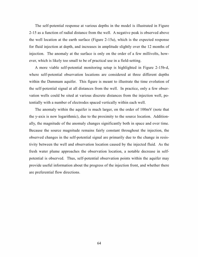
64

The self-potential response at various depths in the model is illustrated in Figure

2-15 as a function of radial distance from the well. A negative peak is observed above

the well location at the earth surface (Figure 2-15a), which is the expected response

for fluid injection at depth, and increases in amplitude slightly over the 12 months of

injection. The anomaly at the surface is only on the order of a few millivolts, how-

ever, which is likely too small to be of practical use in a field-setting.

A more viable self-potential monitoring setup is highlighted in Figure 2-15b-d,

where self-potential observation locations are considered at three different depths

within the Dammam aquifer. This figure is meant to illustrate the time evolution of

the self-potential signal at all distances from the well. In practice, only a few obser-

vation wells could be sited at various discrete distances from the injection well, po-

tentially with a number of electrodes spaced vertically within each well.

The anomaly within the aquifer is much larger, on the order of 100mV (note that

the y-axis is now logarithmic), due to the proximity to the source location. Addition-

ally, the magnitude of the anomaly changes significantly both in space and over time.

Because the source magnitude remains fairly constant throughout the injection, the

observed changes in the self-potential signal are primarily due to the change in resis-

tivity between the well and observation location caused by the injected fluid. As the

fresh water plume approaches the observation location, a notable decrease in self-

potential is observed. Thus, self-potential observation points within the aquifer may

provide useful information about the progress of the injection front, and whether there

are preferential flow directions.

65

Figure 2-1: Coupled forces and fluxes [adapted from Wurmstich, 1995; Bader, 2005] (top). Pictorial representation of the coupling of flows and the development of counter forces in a system [from Marshall and Madden, 1959] (bottom).

66

Figure 2-2: Schematic of the electrical double layer in the vicinity of a solid-fluid interface. The negatively charged solid surface is balanced by fixed positive ions within the Helmholtz layer, and a diffuse layer of ions farther from the interface (top). The potential as a function of distance from the fluid-solid interface decays exponen-tially in the diffuse layer (bottom).

67

Figure 2-3: Cross-section of a cylindrical pore (length l, radius a) with Poiseuille flow due a hydraulic pressure difference ( P∆ ) from top to bottom. The streaming current ( kj ) due to drag of excess charge is balanced by a conduction current ( cj ) in the opposite direction, resulting in an electric potential difference ( V∆ ) across the cylinder.

68

Figure 2-4: Model geometries and boundary conditions for synthetic electrokinetic coupling examples. A) fluid and electric flows are confined to the same domain, where fluid flow is caused by an applied pressure difference across the sample. B) An electrically conductive layer is added to the model, but fluid flow is restricted to the same domain as A).

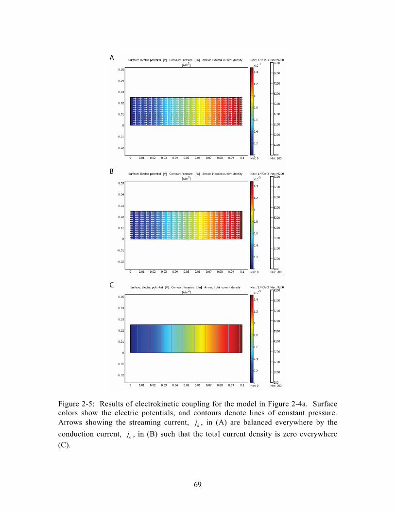
69

Figure 2-5: Results of electrokinetic coupling for the model in Figure 2-4a. Surface colors show the electric potentials, and contours denote lines of constant pressure. Arrows showing the streaming current, kj , in (A) are balanced everywhere by the conduction current, cj , in (B) such that the total current density is zero everywhere (C).

70

Figure 2-6: Results of electrokinetic coupling for the model in Figure 2-4b with -1(2) 0.01 S mr rσ σ= = ⋅ . Surface colors show the electric potentials, and contours de-

note lines of constant pressure. Arrows showing the streaming current, kj , in the lower portion of the model (A) are balanced by the conduction current, cj , in the en-tire domain (B) such that the total current density in (C) through any vertical slice is zero, but is non-zero at any given location.

71

Figure 2-7: Results of electrokinetic coupling for the model in Figure 2-4b with -1(2) 0.001 S mr rσ σ= = ⋅ . Surface colors show the electric potentials, and contours

denote lines of constant pressure. Arrows showing the streaming current, kj , in the lower portion of the model (A) are balanced by the conduction current, cj , in the en-tire domain (B) such that the total current density in (C) through any vertical slice is zero, but is non-zero at any given location.

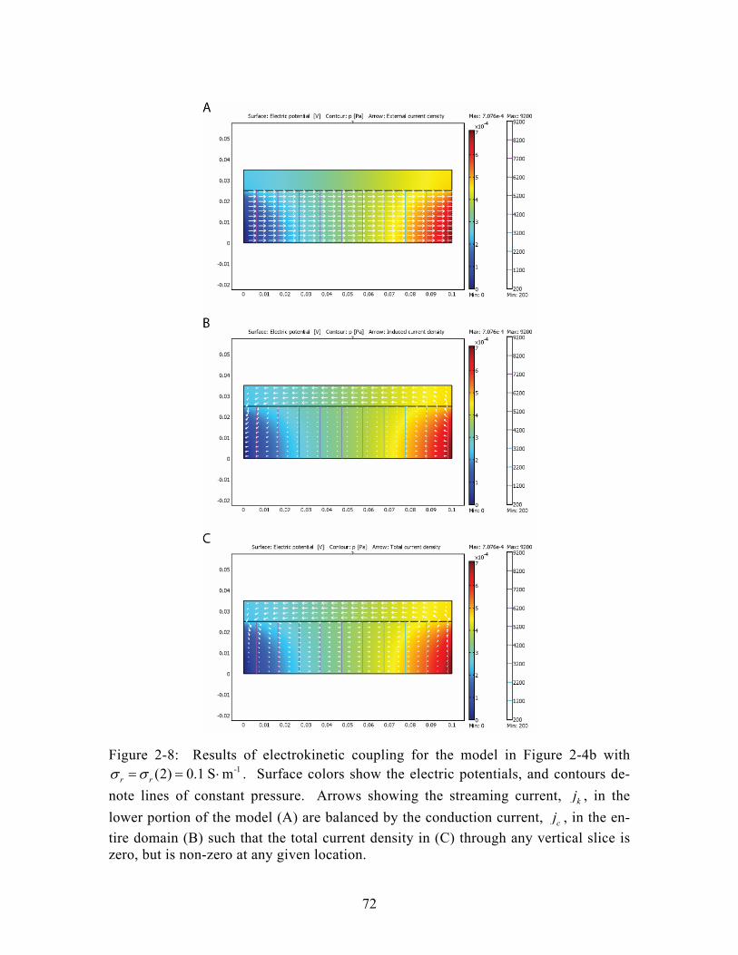
72

Figure 2-8: Results of electrokinetic coupling for the model in Figure 2-4b with -1(2) 0.1 S mr rσ σ= = ⋅ . Surface colors show the electric potentials, and contours de-

note lines of constant pressure. Arrows showing the streaming current, kj , in the lower portion of the model (A) are balanced by the conduction current, cj , in the en-tire domain (B) such that the total current density in (C) through any vertical slice is zero, but is non-zero at any given location.

73

Figure 2-9: Maximum electric potential drop across the model in Figure 2-4b for a fixed applied hydraulic pressure difference as a function of the upper-to-lower layer conductivity ratio. The limiting case where the upper layer conductivity becomes small produces the potential difference predicted by equation (2.26).

74

Figure 2-10: (A) Schematic of a Galvanic cell that can spontaneously produce a cur-rent through an external load (Rcell) due to the difference in equilibrium potential of the different metals. (B) Schematic of a corrosion cell that can spontaneously pro-duce a current due to differences in ionic concentration or oxygen availability in the electrolyte near the top and bottom of the metal.

75

Figure 2-11: Self-potential model surrounding an ore body from Sato and Mooney [1960, Fig. 2].

76

Figure 2-12: Porosity model for the synthetic aquifer storage and recovery hydrogeo-physical modeling. The geometry, aquifer properties, and injection parameters are an approximation for the planned ASR experiment in Kuwait.

77

Figure 2-13: Modeled bulk electrical resistivity before (A) and after 12 months of (B) fresh water injection into the Dammam aquifer. Background variations in resistivity are due to the use of Archie’s Law to compute bulk resistivity from fluid resistivity and porosity.

78

Figure 2-14: Individual terms describing the self-potential sources from equation (2.50) for the aquifer injection model. The major contribution to the source comes from the fluid injection at the well, rather than flow across boundaries in the coupling coefficient.

79

Figure 2-15: Self-potential response at the surface of the aquifer storage model (A) and three depths within the Dammam aquifer (B-D) as a function of distance from the well after 1, 6, and 12 months of injection. Note the different axis scales for (A) and (B-D).

81

Chapter 3

Self-potential source inversion

3.1 Introduction

Source inversion for potential-field problems has been the focus of many geophysical

studies including gravity [Last and Kubik, 1983; Li and Oldenburg, 1998], magnetics

[Li and Oldenburg, 1996; Portniaguine and Zhdanov, 2002], and self-potentials

[Fitterman and Corwin, 1982; Fournier, 1989; Patella, 1997; Birch, 1998; Shi, 1998;

Gibert and Pessel, 2001; Sailhac and Marquis, 2001; Darnet et al., 2003; Revil et al.,

2003a; Rizzo et al., 2004]. Analogous work has also been carried out in the medical

community which uses the electroencephalogram (EEG) to non-invasively measure

time varying electrical potentials on the scalp. The scalp potentials are combined

with resistivity information to spatially and temporally locate electrical sources within

the brain [Pascual-Marqui et al., 1994; Malmivuo et al., 1997; Weinstein et al., 2000;

Michel et al., 2004]. Although different in their application, all of these problems are

governed by an elliptic partial differential equation. Each involves the measurement

of a potential field (or its gradient) that can either be interpreted directly in data-

space, or inverted to determine a source model that predicts the data using the under-

lying physics of the problem.

This chapter provides a methodology for the inversion of self-potential data to

produce an electrical current source model. These current sources can be generated

directly by an electrical source, or through a variety of coupling phenomena (elec-

82

trokinetic, electrothermal, or electrochemical) [Onsager, 1931; de Groot, 1951; Nour-

behecht, 1963]. This work focuses on the inversion problem; it does not attempt to

discuss in detail the relationship between current sources and coupled flow properties,

which can be found in numerous articles [Sato and Mooney, 1960; Fitterman, 1979a;

Sill, 1983; Morgan et al., 1989; Wurmstich and Morgan, 1994; Wurmstich, 1995; Re-

vil et al., 1999a; Naudet et al., 2003; Revil et al., 2003b; Darnet et al., 2004], and is

also discussed in Chapter 2.

Source inversion is fundamentally different from tomographic inverse problems,

which seek to describe the spatial variation in physical properties such as velocity or

resistivity. Sources tend to be spatially localized, though the actual smoothness of the

distribution of sources varies for different problems. Several inversion techniques

have been developed to account for the compact nature of sources [Last and Kubik,

1983; Portniaguine and Zhdanov, 1999]. Our approach combines these concepts

with inverse sensitivity scaling techniques that have been effective in many geophysi-

cal inverse problems [e.g. Li and Oldenburg, 1996]. The sensitivities are calculated

according to the reciprocity theorem, which allows for complex resistivity structure

and model geometry. Reciprocity is an efficient way to calculate the Green’s func-

tions for the source inverse problem because the solution relies only on multiple well-

posed forward calculations [Penfield et al., 1970; Madden, 1972; Malmivuo et al.,

1997].

Accurate determination of the 3D distribution of current sources that describe the

self-potential signal provides valuable information about the causal coupling proc-

esses. We discuss how accurate calculation of the source distribution is complicated

because measured SP data are affected by unknown (or imperfectly estimated) resis-

tivity structure. All of the examples used to demonstrate these concepts are three di-

mensional, though simple 1D or 2D geometries are used for the purpose of illustra-

tion. This work follows that of Zhang et al. [1995] and Shi [1998], who utilize the

transmission network analogy and conjugate gradient algorithms to solve the forward

and inverse problems.

83

3.2 The electric forward problem

Equation (2.11), repeated below, is an elliptic partial differential equation that governs

the dc electrical response due to a source in a conductive medium.

−∇ ⋅ ∇ =σ φ s (3.1)

σ represents the earth conductivity structure [S·m-1], φ is the electrical potential [V],

and s describes the electrical current source density [A·m-3] forcing term. This is

simply a statement of the conservation equation applied to the current density field

= − ∇j σ φ [A·m-2]. Mathematically, it is the same expression that applies to the elec-

trical resistivity geophysical method [e.g. Telford et al., 1990], which uses known

sources (electrodes) and measured potentials to recover the earth resistivity structure.

In this thesis, the self-potential forward problem refers to the calculation of φ ,

given s and σ . The forward response in equation (3.2) is defined by the spatial con-

volution of the source term s and Green’s functions φG.

( ) ( ) ( ); ,Gx x x x dxσ′ ′ ′= ∫φ φ sD

(3.2)

For the self-potential inverse source problem, measured potentials are combined with

assumptions about the earth resistivity structure in order to recover the unknown

sources. Solution of the inverse problem, which is discussed further in this chapter,

requires multiple solutions of the forward problem.

Mixed boundary conditions are used in conjunction with equation (3.1). A Neu-

mann boundary condition is specified at the air-earth interface, such that 0⋅ ∇ =n σ φ .

Within the earth, a Dirichlet boundary condition requires that 0→φ as the distance

from the sources becomes large ( r → ∞ ). This typically requires that the model

boundaries are far away from the source region of interest [Dey and Morrison, 1979].

The calculation of φ, given s and σ, is a well-posed forward problem and can be

accomplished with a variety of numerical algorithms. The finite element package,

COMSOL MultiphysicsTM 3.2, was utilized in the previous discussions of self-

potential mechanisms to solve equation (3.1). There are two significant benefits to

this package: (1) flexibility for incorporating complicated model geometries and (2)

84

the multiphysics approach that allows the physics of the source mechanism to be cou-

pled directly into the problem. One drawback, however, is that it is not ideally

adapted for use within the inverse problem, which requires fast solutions of many

forward problems.

In this thesis I adapt a code developed originally for resistivity problems, but

modified by Shi [1998] to solve the self-potential inverse problem. This code utilizes

the transmission network analogy [Madden and Swift, 1969; Madden, 1972] to solve

equation (3.1), which involves the discretization of the model into network nodes and

impedance branches, and is reviewed in more detail in Appendix A. Potentials and

current sources are defined at each node. In three-dimensions, each interior node is

connected to the six surrounding nodes by impedance branches. The impedances [Ω]

are calculated from resistivity [Ω·m] values given at the node locations and the dis-

tance between nodes. This is analogous to a network of resistors, where currents [A]

flow through the branches [Ω], and potentials [V] are defined at all intersections.

Kirchoff’s law requires that flow into any node equals the flow out of that node in the

absence of a current source.

Equation (3.1) can be redefined in terms of the transmission network as a linear

system of equations (3.3), where the discretized forcing term, s, on the right hand side

now has units of current, [A].

Kφ = s (3.3)

A useful property of K is that it is positive definite symmetric, and therefore has

an inverse. Direct calculation of K-1, which is a full matrix, is prohibitive for most

3D problems with even modest dimensions. Efficient calculation of the forward prob-

lem is essential for solving the inverse problem, and can be accomplished using vari-

ous algorithms. The code developed in this study uses a conjugate gradient algorithm

with incomplete Cholesky decomposition and sparse storage to calculate the vector of

potentials, φ, given K and s; thereby avoiding storage of the matrix inverse. Zhang et

al. [1995] and Shi [1998] provide a useful account of the forward problem through the

use of the transmission network and conjugate gradients.

85

3.3 The inverse problem

The self-potential inverse problem involves the calculation of s throughout the model

from an incomplete set of measured potentials and known or estimated impedances.

As a DC geoelectric problem, the impedance is a function of the model resistivity and

geometry, and there is no complex component. There are two fundamental difficulties

that are addressed during the inversion. The first problem involves the large varia-

tion in sensitivity of the data to different model parameters. The sensitivity is typi-

cally greatest near the measurement locations, though it is also a function of the resis-

tivity structure. Sensitivity scaling is therefore applied by defining a weighting op-

erator that is calculated from the cumulative sensitivity of each model parameter to all

of the measured data. Second, this is an ill-posed problem with a fundamentally non-

unique solution, which is compounded by the limited set of available measurements.

In order to address this non-uniqueness, we choose to select a class of source solu-

tions that have a desired spatial compactness. This choice amounts to the addition of

prior knowledge about the properties of s, which may be dependant on the particular

problem of interest.

Equation (3.4) states the basic inverse problem, where K† represents K-1 using

conjugate gradients to avoid direct calculation and storage of the inverse.

†K s = φ (3.4)

We assume that the earth resistivity structure, which is part of K, is known. Ideally,

the results of a resistivity survey should be incorporated into the self-potential inver-

sion. Errors in the resistivity structure will clearly propagate as an error in the source

estimate. The sources, s, could theoretically be calculated if φ is known completely,

but in practice this will never be the case. φ is typically sampled at a limited subset

of locations (N << M) that are often limited to the surface of the earth. Equation (3.5)

gives the more common situation, where the N measured potentials, φd, are related to

the M unknown sources through a subset of the rows of K† selected by the N by M

matrix operator P. P is a ‘selector’ matrix that consists of a single ‘1’ on each row in

the column that corresponds to the measurement location.

86

†dPK s = φ (3.5)

Each row of K† contains the Green’s function that multiplies the source vector and

results in a potential. Multiplication by P selects only the Green’s functions related to

the measurement locations. We discuss below how the Green’s functions for an arbi-

trary resistivity structure are calculated using reciprocity. Because PK† has many

more columns than rows, it is rank-deficient and the problem is ill-posed. Including

more measurements, which incorporates more rows of K†, improves the source recon-

struction. The solution that minimizes the l2 norm of the data misfit,

( ) 2†

2d d dφ = −W PK s φ , (3.6)

is given in equation (3.7), which relies on the symmetry of K† (i.e. the Green’s func-

tions are self-adjoint, and K-1=K-T)

† 2 † †T Td d(K P W PK )s = K P φ . (3.7)

In practice, dW typically contains information about the standard deviation of the

measurement errors, but for the purpose of simplifying the remaining discussion

d =W I .

The utility of a conjugate gradient algorithm to estimate s without computing ma-

trix inverses is evident from equation (3.7). All that is required to find s is a series of

matrix-vector products [Rodi, 1976; Mcgillivray and Oldenburg, 1990; Zhang et al.,

1995]. K† operating on a ‘source’ vector is simply the solution to the well-posed for-

ward problem (3.3), which provides a set of ‘potentials’ also found using conjugate

gradients. The quotes are used because the vectors do not necessarily represent real

sources and potentials. For instance, PTφd is the ‘source’ vector on the right side of

the equation from which a vector of ‘potentials’ are calculated. This represents a

back-projection of the data into model-space. On the left side of the equation there is

a forward calculation, multiplication by the selection operator P and its transpose, fol-

lowed by a second forward calculation. Thus, the source estimate is found through a

series of forward calculations nested within a conjugate gradient algorithm. In prac-

87

tice, the ill-conditioning of this problem requires that additional model regularization

is used.

3.4 Sensitivity scaling

Sensitivity scaling requires calculation of the Jacobian (J), or sensitivity of the data

with respect to the model parameters (3.8).

( )† †T

T T Td∂ ∂= = =

∂ ∂φJ s K P K Ps s

(3.8)

By our definition, PT consists of N column vectors with a single 1 in each column

corresponding to the data locations. Computation of J is therefore accomplished

through N forward calculations using a unit source at each data location, which is an

efficient way to calculate the sensitivity kernel for this problem, as illustrated by

equation (3.9). Note that the resistivity structure is already included in K, and is

therefore naturally incorporated into the sensitivity calculation.

1 11

11 1†

1

1

N

NTTd

N M M

NM M

s ss s

s ss s

ϕ ϕ ϕϕ

ϕ ϕ ϕϕ

∂ ∂ ∂∂⎛ ⎞ ⎛ ⎞⎜ ⎟ ⎜ ⎟∂ ∂∂ ∂⎜ ⎟ ⎜ ⎟∂ ⎜ ⎟ ⎜ ⎟= = =

∂ ⎜ ⎟ ⎜ ⎟∂ ∂ ∂∂⎜ ⎟ ⎜ ⎟⎜ ⎟ ⎜ ⎟∂ ∂∂ ∂⎝ ⎠ ⎝ ⎠

φ K Ps

……

(3.9)

Each column on the left of (3.9) gives the sensitivity of one datum to all parame-

ters, which is found on the right side by calculation of the potentials at every location

due to a unit source at the datum location. This is a statement of reciprocity, which

states that the sources and receivers can be exchanged (3.10).

TTji

j is sϕϕ ∂∂

=∂ ∂

(3.10)

In this study, J is not used directly in equation (3.7); rather, it is used to calculate

the cumulative sensitivity of the data to each parameter. The cumulative sensitivity is

similarly defined by Portniaguine and Zhdanov [1999], and is given by (3.11).

88

1/ 2

2

1

1:N

kk kjj

J k M=

⎛ ⎞Λ = =⎜ ⎟

⎝ ⎠∑ … (3.11)

The Λkk form a diagonal weighting matrix that is used in the model regularization

term in the new objective function given by equation (3.12). This weighting allows

for solutions away from the measurement locations, typically at depth, where sensitiv-

ity is decreased. Similar weighting schemes have been used in gravity [Li and Olden-

burg, 1998; Boulanger and Chouteau, 2001] and magnetic [Li and Oldenburg, 1996;

Pilkington, 1997] inverse problems.

2 2†

22d m dφ λφ λΦ = + = +PK s -φ Λs (3.12)

Here, λ is a trade-off parameter that controls the relative influence of the data and

model misfit terms. It is convenient to make a transformation, ws = Λs , and rewrite

(3.12) in terms of the weighted variable sw (3.13).

2 2† 1

22w w d wλ−Φ = +PK Λ s -φ s (3.13)

Minimization of the weighted objective function with respect to sw leads to equation

(3.14).

( )1 † † 1 1 †T Tw dλ− − −+ =Λ K P PK Λ I s Λ K P φ (3.14)

Equation (3.14) can be solved in the same way as described for equation (3.7),

through forward operations applied to a ‘source’ vector and multiplication by several

sparse matrices within a conjugate gradient algorithm. The solution for sw is then

multiplied by the diagonal matrix Λ-1 to recover s. The effect of the Λ-1 term in (3.14)

becomes clear: it scales the left-most term such that the diagonals are equal to one.

By equalizing the diagonals, parameters with large sensitivities do not dominate, and

solutions can be found away from the measurement locations.

According to equation (3.12), this method simply involves a solution that is con-

strained by data misfit and a sensitivity-weighted minimum length term. Other model

regularization operators (i.e. gradient or Laplacian) can also be used to produce flat or

89

smooth models. In practice, a data weighting term with estimated variance informa-

tion can also be applied, but is excluded here for clarity.

3.5 Model regularization for self-potential source in-version

As discussed by Constable et al. [1987], the purpose of regularization in the inverse

problem is to introduce stability while recovering models that do not contain more

complicated features than are justified by the data. A common form of regularization

involves the measure of a low order differential operator applied to the model [e.g.

Tikhonov and Arsenin, 1977]. Minimization of this functional using an l2 norm results

in a linear system of equations that introduces stability through the constraints pro-

vided by the regularization operator. Thus, the regularization term in equation (3.12)

is of the form

2

2m mφ = W s . (3.15)

When the operator is the identity matrix ( m =W I , 0th order), a minimum length

solution is obtained. Other popular operator choices include the gradient ( m = ∇W ,

1st order) or Laplacian ( 2m = ∇W , 2nd order), which produce flat or smooth solutions,

respectively. Additional a-priori information can be included, for example, by intro-

ducing anisotropic weights for the gradient operator to promote features such as hori-

zontal layering. Li and Oldenburg [1996; 2000] employ a combination of metrics that

enforce a minimum length solution with respect to a reference model, allow for ani-

sotropic spatial gradients, and incorporate depth weighting to overcome problems re-

lated to poor sensitivity at depth. The sensitivity scaling techniques discussed in the

previous section can be included with any of these linear operators.

These methods are widely used because inversion stability and reasonable model

constraints are introduced in a framework that fits naturally with least squares algo-

rithms, i.e. the objective function involves a quadratic function of the model. The re-

sulting models, however, tend to have smooth variations that may not always be

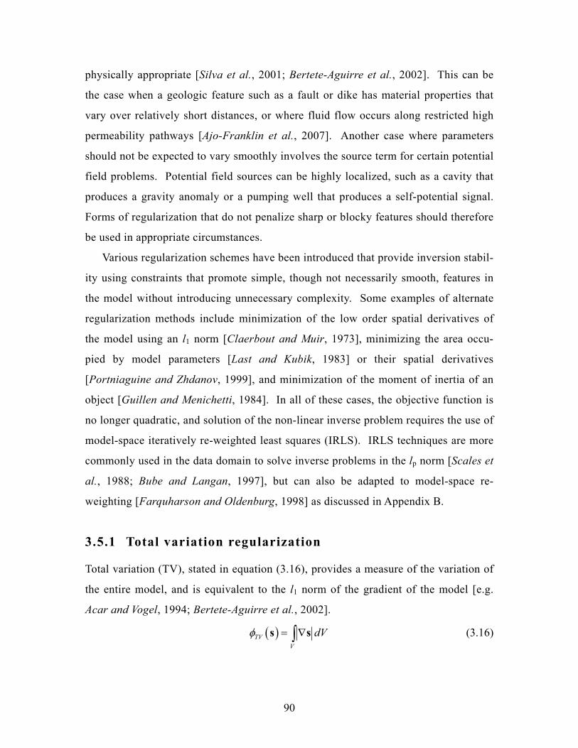
90

physically appropriate [Silva et al., 2001; Bertete-Aguirre et al., 2002]. This can be

the case when a geologic feature such as a fault or dike has material properties that

vary over relatively short distances, or where fluid flow occurs along restricted high

permeability pathways [Ajo-Franklin et al., 2007]. Another case where parameters

should not be expected to vary smoothly involves the source term for certain potential

field problems. Potential field sources can be highly localized, such as a cavity that

produces a gravity anomaly or a pumping well that produces a self-potential signal.

Forms of regularization that do not penalize sharp or blocky features should therefore

be used in appropriate circumstances.

Various regularization schemes have been introduced that provide inversion stabil-

ity using constraints that promote simple, though not necessarily smooth, features in

the model without introducing unnecessary complexity. Some examples of alternate

regularization methods include minimization of the low order spatial derivatives of

the model using an l1 norm [Claerbout and Muir, 1973], minimizing the area occu-

pied by model parameters [Last and Kubik, 1983] or their spatial derivatives

[Portniaguine and Zhdanov, 1999], and minimization of the moment of inertia of an

object [Guillen and Menichetti, 1984]. In all of these cases, the objective function is

no longer quadratic, and solution of the non-linear inverse problem requires the use of

model-space iteratively re-weighted least squares (IRLS). IRLS techniques are more

commonly used in the data domain to solve inverse problems in the lp norm [Scales et

al., 1988; Bube and Langan, 1997], but can also be adapted to model-space re-

weighting [Farquharson and Oldenburg, 1998] as discussed in Appendix B.

3.5.1 Total variation regularization

Total variation (TV), stated in equation (3.16), provides a measure of the variation of

the entire model, and is equivalent to the l1 norm of the gradient of the model [e.g.

Acar and Vogel, 1994; Bertete-Aguirre et al., 2002].

( )TVV

dVφ = ∇∫s s (3.16)

91

Minimization of the total variation functional generates “blocky” images that are

piecewise constant over one or more regions [Claerbout and Muir, 1973; Dobson and

Santosa, 1996]. Both l1 and l2 norms of the gradient penalize oscillations in the

model due to noisy data, but sharp discontinuities are better preserved under the l1

norm. Total variation has been applied in various forms to geophysical inverse prob-

lems [Claerbout and Muir, 1973; Portniaguine and Zhdanov, 1999; Yu and Dough-

erty, 2000; Bertete-Aguirre et al., 2002], and has also been developed for noise sup-

pression in image processing [Rudin et al., 1992; Acar and Vogel, 1994; Vogel, 2002].

Because equation (3.16) is non-differentiable when any of the 0is∇ = , the total

variation functional is often approximated using equation (3.17) [e.g. Farquharson

and Oldenburg, 1998; Bertete-Aguirre et al., 2002].

( ) ( )1/ 22 2TVφ β= ∇ +s s (3.17)

This is a specific case of the generalized measures of data misfit and model structure

discussed by Farquharson and Oldenburg [1998], and is also reviewed in Appendix

B. The gradient operator is replaced with its discrete form of the differencing opera-

tor such that m = ∇W . Differentiating equation (3.17) with respect to s leads to

( )TV Tm m

φ∂=

∂s

W RW ss

(3.18)

where,

( )( ) 1/ 22 2ii m i

R β−

= +W s . (3.19)

R is a diagonal matrix with an entry for differences between adjacent model parame-

ters in all directions, and β provides stability when the model gradient is near zero.

Minimization of the full objective function, d TVφ λφΦ = + , results in the familiar sys-

tem of equations for s given in equation (3.20).

( )† † 1 †T T j j Tm m dλ −+ =K P PK W R W s K P φ (3.20)

An iterative solution method must be used because the total variation constraint

involves a non-linear function of the model. The first estimate, s1, typically comes

92

from a conventional linear smoothness constraint by setting 0 =R I . This model is

then used to compute a new diagonal weighting matrix 1j−R and, subsequently, a new

model estimate, js . The solution that satisfies the total variation constraint is reached

when changes to the model become sufficiently small, i.e. 1j js s ε−− < .

3.5.2 Spatially compact sources using minimum support regularization

For the potential-field source inversion problem, a constraint that requires the source

model to be spatially localized has more meaning: a self-potential source due to well

pumping will be near the screened portion of the well, a gravity anomaly due to an

intrusion is limited to the area of change in density, etc. Elsewhere, the source term

should be zero. Wurmstich [1995] illustrated the localization of self-potential sources

by computing the electric power density for several synthetic models, where the

power density drops off rapidly from the source locations.

Compact source constraints have proven useful in various geophysical and medi-

cal investigations [Last and Kubik, 1983; Portniaguine and Zhdanov, 1999; Portni-

aguine et al., 2001; Silva et al., 2001; Portniaguine and Zhdanov, 2002]. Different

inverse problems will involve a range of model characteristics such as compactness or

smoothness; therefore, a regularization operator should be chosen that incorporates

the intrinsic physical properties of interest. Portniaguine and Zhdanov [1999] discuss

a minimum support stabilizing functional that is developed from the compactness

constraint used by Last and Kubik [1983]. This is based on the minimization of an

area (or volume in three-dimensions) metric given by equation (3.21).

2

2 20 1

limM

ke

k k

sarea asβ β→

=

=+∑ (3.21)

Here, ae represents the area of an individual model block or element, which is as-

sumed constant in this case. β is a small number that is introduced to provide stability

as sk → 0. In the limit of β → 0, terms in equation (3.21) evaluate to 1 for any value

of sk ≠ 0, and they become 0 for sk = 0. This metric approximates the area of the

93

anomalous region, and is essentially the same as the minimum support functional dis-

cussed by Portniaguine and Zhdanov [1999].

A new objective function is defined that incorporates the measure of area,

22†

2 221

Mk

d m dk k

ss

φ λφ λβ=

Φ = + = ++∑PK s -φ . (3.22)

Figure 3-1a shows the general form of the model regularization term ( mφ ) for several

values of β compared with the traditional damping case where =Λ I in equation

(3.12). The compactness term is clearly non-quadratic, though large values of β

(relative to ks ) introduce a similar damping effect on the model parameters. For the

case when ksβ , the compactness constraint becomes apparent; the objective term

asymptotes to one regardless of the magnitude of ks . Hence, the penalty on model pa-

rameters does not depend on their relative magnitude, only whether or not they lie

above or below the threshold of β . Minimization of mφ is realized by allowing the

greatest number of parameters to have amplitude less than β . Large absolute values

of the remaining parameters are not constrained since any value greater than β evalu-

ates to ~1.

A new weighting variable is defined by equation (3.23), which includes the mini-

mum support functional scaled by the cumulative sensitivity weights, which is con-

ceptually similar to R in equation (3.19).

( 1)

1/ 22

2 2 1:j

kkkk

k

k Ms β

−

⎛ ⎞Λ⎜ ⎟Ω = =⎜ ⎟+⎝ ⎠

… (3.23)

The denominator of kkΩ is fixed with respect to a prior model (j–1) so that the regu-

larization term becomes a quadratic function of the unknown parameters, sk, and can

be easily incorporated into a traditional least squares algorithm.

2 2†

22MS d m dφ λφ λΦ = + = +PK s -φ Ωs (3.24)

In other words, the estimate of s that minimizes the minimum support objective

function fits the data using the fewest number of parameters, scaled by the cumulative

94

sensitivity. Because the prior estimate of s is used in equation (3.23), this minimiza-

tion occurs in the neighborhood of 1j−s . This formulation allows the linear inversion

to be repeated using an IRLS approach, with a new Ω calculated at each step from the

previous s. Each successive optimization reduces the minimum support functional by

using fewer parameters until further reduction no longer fits the data and 1j j−≈s s . In

general, as fewer parameters are used to fit the data, the source parameters must in-

crease in amplitude and move to greater depth.

Figure 3-1b shows the linearized form of the model regularization term, which

now depends on the value of a prior model estimate, 1jks − . First, note that even for

small values of β (relative to 1jks − ) the objective function does not asymptote to a

constant value as in Figure 3-1b. In this case where 1jksβ − , it is the ratio 1j j

k ks s −

that is penalized quadratically. When 1jksβ − , the objective term simplifies to the

traditional damping case and β serves to bound the values of elements on the diago-

nal of Ω ; as 0ks → , kk kk βΩ → Λ . At any given step, Ω can be viewed as a spa-

tially variable damping matrix with high values in regions where the prior model es-

timate has a small absolute magnitude. This promotes compactness, and reduces un-

necessary model complexity, by damping out relatively small amplitude features,

within the constraints provided by the data misfit term.

Using the transformed parameters, w =s Ωs , the form of the solution similar to

(3.14), the only difference being the numerator of Ω-1 that now scales the left most

term of (3.25).

( )1 † † 1 1 †T Tw dλ− − −+ =Ω K P PK Ω I s Ω K P φ (3.25)

Once computed, sw is then transformed back to the original parameters using 1

w−s = Ω s .

It is important to remember that the compact source solution does not remove the

inherent non-uniqueness for this problem. Instead, this method finds an ensemble of

source solutions that fit the data equally using increasingly compact models. The in-

95

terpreter must still decide which solution is ‘correct’ based on prior information about

the source properties. One effective stopping criterion might be a pre-specified model

roughness, which tends to increase as the solution becomes more compact.

3.5.3 The role of multiple regularization parameters

Zhdanov and Tolstaya [2004] and Farquharson and Oldenburg [1998] discuss

how to choose an appropriate value for β based on a tradeoff curve method. This is

accomplished by plotting β versus mφ for multiple values of β and a given model.

Small values of β lead to small values of mφ , but may introduce instability or un-

wanted oscillations in the model, especially when noise is present in the data. As β

becomes large, the minimum support functional behaves more like a weighted mini-

mum length constraint. Thus, β can be chosen from the tradeoff curve such that it

controls the behavior of the regularization term, providing a balance between desired

compactness and stability.

A further complication, however, is that there are now two regularization parame-

ters that control the solution, λ and β, which cannot be chosen independently. In or-

der to understand the combined influence of these parameters, a synthetic dataset is

generated from a known source and is contaminated with zero-mean Gaussian noise.

These data are then inverted using equation (3.25) and 99 different combinations of

fixed values for the regularization parameters, i.e. all combinations of nine logarith-

mically equi-spaced values of λ between 1x10-4 and 1x101, and eleven logarithmically

equi-spaced values of β between 1x10-3 and 1x10-1.

In Figure 3-2, an L-curve [e.g. Hansen and Oleary, 1993] is displayed for each

value of β, and points along each curve represent different values of λ. The L-curve

represents the tradeoff between the model norm ( mφ ) and the data norm ( dφ ). For a

single curve, one generally selects the value of λ at the point of maximum curvature,

thereby finding the solution that minimizes both terms optimally. For display pur-

poses, the x-coordinate in Figure 3-2 is 2mβ φ instead of simply mφ . Because

96

( )2 0mβ φ β∂ ∂ > , the curves do not overlap and β increases from the left-to-right of

the figure, where smaller β correspond to more “compact” solutions. Large values of

β decrease the model norm as determined by equation (3.22), but do not lead to com-

pact solutions. The true level of noise added to the dataset is annotated by the black

dashed line.

The curves on the right side of Figure 3-2 correspond to smooth solutions and

have the traditional “L-shape”. Pre-multiplication of the model norm by β2 has the

effect of collapsing all of these curves together because β2 is the dominant term in the

denominator of (3.22). As β decreases, however, the effect of the minimum support

operator takes over and the model norm decreases because solutions become increas-

ingly compact. The three left-most curves in Figure 3-2 exhibit equal degrees of

compactness (for a given level of data misfit), but appear separated on the figure due

to the pre-multiplication by β2. The combined effects of λ and β are summarized in

Table 3-1 below, where the four quadrants in the table roughly correspond to the re-

gions in Figure 3-2.

Table 3-1: Summary of the combined influence of the minimum support regulariza-tion parameters

Small β Large β

Large

λ

Solutions are compact. For increas-

ing λ, the IRLS method compacts

the solution too rapidly, leading to

an incorrect source location and

therefore increasingly poor data fit.

Solutions are smooth. For increas-

ing λ, the data norm becomes large

because smoothness is favored over

data fit.

Small

λ

Solutions have an intermediate de-

gree of compactness. Small λ al-

lows the data to be over-fit, requir-

ing numerous sources near the

measurement locations

Solutions are relatively smooth, but

there may be significant oscillations

near the receivers required to fit the

noise in the data.

97

Figure 3-2 highlights an important result; it illustrates that the nonlinear minimum

support regularization term behaves as a stabilizing functional should, providing a

tradeoff between data misfit and a measure of model length. It is interesting to note,

for this example, that the notch in the “L” falls at or near the correct level of data mis-

fit for the compact solutions (three left-most curves). The fact that there is an addi-

tional regularization parameter complicates the situation somewhat, but the behavior

of the solution can be predictably controlled by the selection of λ and β.

3.5.4 Synthetic illustration of various regularization tech-niques

A simple two-dimensional synthetic example is used to illustrate the different types of

results achieved with the regularization methods discussed thus far. Figure 3-3a

shows the “true” 2D source model, which consists of a negative point source with

amplitude -3mA and a positive dipping source with pixel amplitudes +1.5mA. The

resistivity structure is homogeneous, and a dense set of measurement locations are

shown at the top of the model with black triangles. Synthetic noise-free data gener-

ated from this model are displayed in Figure 3-3b. This model is roughly representa-

tive of the source characteristics that might be described by equation (2.50); a point-

like source near the location of fluid injection/extraction in a well, and a linear source

feature where there is flow across a boundary in the coupling coefficient.

Figure 3-4 shows the source inversion results using the traditional linear regulari-

zation techniques, where m =W I in Figure 3-4a, m = ∇W in Figure 3-4b, and

2m = ∇W in Figure 3-4c. Sensitivity scaling, as discussed in section 3.4, is also in-

cluded for all three cases, and λ is fixed at 0.1. All of the models using traditional

regularization are very smooth, and do not capture much information about the true

source structure (which is depicted by white asterisks).

Results using the total variation regularization technique are shown in Figure 3-5,

again with λ fixed at 0.1. The initial model for the iterative procedure is the smooth

model from Figure 3-4c. The solutions are illustrated at IRLS iterations #3 (Figure

98

3-5a), #5 (Figure 3-5c), and #7 (Figure 3-5e). In addition to the source solutions, the

diagonal elements of the regularization term in equation (3.20), i.e. Tm mW RW , com-

puted from the solutions at these iterations are illustrated in Figure 3-5b, Figure 3-5d,

and Figure 3-5f. These maps of the regularization operator can be viewed as a spa-

tially variable damping operator, where small values correspond to a weak constraint

on model amplitudes and large values correspond to a stronger constraint. The total

variation results provide a slight improvement over the traditional regularization

methods in that the anomalous regions are better localized about the true source loca-

tions. As expected, this solution is “blockier” than the traditional result, but is still

not able to completely reconstruct the true source model.

Next, the compact source solution using the minimum support regularization tech-

nique is illustrated in Figure 3-6. The starting model is again taken as the smooth

model from Figure 3-4c. Results are shown for IRLS iterations #3 (Figure 3-6a), #5

(Figure 3-6c), and #7 (Figure 3-6e). The weighting operator Ω used to compute each

of these solutions is shown in Figure 3-6b, Figure 3-6d, and Figure 3-6f. The influ-

ence of the spatially variable damping that depends on the amplitude of the prior

model estimate is evident. The large near-surface weights in the background of all of

the weighting operator images comes from the sensitivity scaling term in equation

(3.23). The compact source solution is clearly able to capture the true source struc-

ture and amplitudes, though solutions that are “over-compact” can also be found due

to non-uniqueness and limited data sensitivity. This is partially evident in Figure

3-6e, where the dipping positive source becomes somewhat broken up.

Finally, the influence of noisy measurements is considered for the minimum sup-

port method, which is illustrated in Figure 3-7. Gaussian noise is added to the data in

Figure 3-3b, where the noise has zero-mean and standard deviation equal to 10% of

the mean of the noise-free measurements. Figure 3-7a shows the source inversion re-

sult for the first iteration using the traditional smoothness constraint. The main fea-

tures are similar to Figure 3-4c, but the uncorrelated random noise is manifested pri-

marily as near-surface artifacts. The subsequent minimum support results for itera-

tions #3 (Figure 3-7b) and #5 (Figure 3-7d) are also shown along with the correspond-

99

ing weighting operators (Figure 3-7c and Figure 3-7e, respectively). As the features

become increasingly compact, the true source locations and shapes cannot be recov-

ered due to the influence of the noisy measurements. Subtle features in the data due

to a dipping or distributed source are masked by the noise, limiting the extent to

which these features can be imaged.

It is important not to over-fit the data in the presence of noise, as many shallow

sources are needed to fit rapid oscillations in the data due to random noise. One op-

tion is to choose λ for the first IRLS iteration such that the solution is slightly over-

damped, and artifacts due to the noise are avoided. Alternatively, if the level of noise

in the data is known the target data misfit can be specified accordingly. Subsequent

iterations with increasingly compact solutions are then found that also avoid over-

fitting the noise due to the nature of Ω , which tends to enhance the regions of the

model that have large amplitudes in previous iterations.

Also, as the level of noise in the data increases, the model resolution decreases.

This can be explained by the model resolution matrix, R, where est true=m Rm . For

the traditional linear regularization techniques R is a function of the acquisition ge-

ometry and regularization operator, and is independent of the data. For the minimum

support regularization, however, R depends on a prior model estimate, and is there-

fore data-dependent. Thus as the data quality becomes poorer, one should expect re-

sults with correspondingly lower resolution.

Overall, the minimum support regularization technique provides superior results

for the self-potential source inversion problem. This method works well because it

can be justified that the sources occupy a limited volume in the subsurface, and have

zero magnitude at most locations. Various self-potential source mechanisms will have

different degrees of spatial compactness, however, and so the degree to which a truly

compact source solution is sought should be considered for a given problem. By in-

troducing prior knowledge about the spatial statistics of the source processes, for ex-

ample, one can remove some of the inherent ambiguity regarding how compact the

source structure should be. One approach might incorporate the physics and/or chem-

100

istry of the coupling mechanism in a statistical sense to determine a plausible range of

correlation lengths for the source distribution.

While the total variation approach generates solutions that are more spatially

compact than the traditional smoothness constraint, it does not explicitly seek to

minimize the volume of the causative anomaly. Based on these results, the minimum

support regularization technique is utilized throughout the remainder of this disserta-

tion for the self-potential inverse source problem. Possible improvements might in-

corporate a hybrid minimum support/total variation constraint to seek solutions that

are spatially compact, but avoids oscillation within the anomalous region associated

with “over-compaction” of the anomaly. A drawback of this approach is that it re-

quires multiple user-selected tradeoff parameters, λ.

3.6 3D synthetic example with minimum support regularization

A simple 3D synthetic example is used to illustrate the utility of the methods de-

scribed. The model has dimensions 36 x 46 x 23 (M = 38,088 nodes) with 5m spacing

between nodes, and has a homogeneous 100Ω·m resistivity structure. Two current

sources are located within the volume (Figure 3-8): a negative point source at

(16,16,6) and a positive, dipping source at (20,24-28,4-8). Synthetic data generated

from the current source model are shown in Figure 3-9. The data have been sampled

at N = 60 random surface locations to simulate a typical surface SP survey. The con-

toured data show a clear anomaly over the positive source, but there is little evidence

of its shape or the presence of the negative point source.

These data are first inverted using the basic approach of equation (3.7), with the

addition of a minimum length constraint on the model ( 2min s ) and the correct ho-

mogeneous resistivity. Slices through the resulting model are shown in Figure 3-10a.

As expected, the estimated sources have been pulled towards the surface measure-

ments. Figure 3-10b shows the cumulative sensitivities, as calculated by equations

(3.8) and (3.11). The very low sensitivity near the edges is due to the fact that several

101

padding blocks with much larger node spacing are used, and are therefore very far

from the measurement locations. Incorporating the sensitivity scaling in the inversion

starts to provide better information at depth, which is shown in Figure 3-10c.

Next, equation (3.25) is solved for this example to illustrate the effect of the com-

pactness constraint. Larger values of λ tend to increase the rate that solutions become

more compact, but also tends to produce a less stable result. λ is fixed at 1.0 for this

example. Figure 3-11 shows the iterative re-weighting scheme that produces increas-

ingly compact sources. The top image for each iteration is a slice of the diagonal

weighting terms, Ω, along x = 20. Because the initial source estimate is zero ( 0 0=s ),

the first iteration produces exactly the same weighting and source result as the sensi-

tivity weighted minimum length solution shown in Figure 3-10. From this estimate, a

new weighting term is calculated according to equation (3.23), which is then used to

find a new source estimate. The weighing term and source results for iterations 4 and

7 are shown in Figure 3-11b and c.

The effects of the minimum support functional become clear in these iterations as

the source images become more focused. Relatively weak constraints are imposed on

the parameters where sources were estimated in the previous iteration, and the con-

straint tends towards sensitivity scaling only for the parameters where the previous

source estimation was near zero. Note the different color scale at each iteration; the

source amplitudes increase as their spatial extent decreases, and ultimately reach ap-

proximately 20% of the true amplitude. Table 3-2 summarizes the data misfit and

model norm for these results. Because there is no noise in this synthetic example, the

data misfit is allowed to be small, as can be seen by the <1mV data RMS error. While

the data misfit varies only slightly, the model norm drops rapidly (by four orders of

magnitude) during the minimum support iterations as fewer parameters are used to fit

the data. This highlights the point that the minimum support regularization technique

allows us to find multiple solutions which fit the data equally, but exhibit varying de-

grees of spatial compactness.

The synthetic example given in this study takes about eight minutes to run ten it-

erations on a 2GHz Linux workstation. Calculation of the cumulative sensitivity in-

102

formation involves N forward calculations, but only needs to be calculated once for a

given dataset and model geometry and resolution. This information can then be

stored and read directly for future runs with different inversion parameters.

3.6.1 Effect of unknown resistivity structure

An important source of error in the self-potential inversion comes from the fact that

assumptions about the resistivity structure are incorporated in the operator, K. Ide-

ally, an estimate of this structural information would be provided by a resistivity sur-

vey carried out in conjunction with the self-potential survey, though this is not always

practicable, and is never perfect. In this section, several synthetic examples are illus-

trated where the true resistivity structure is unknown, and a homogeneous value is

used for the inversion. This provides useful insight for interpreting source inversion

results that are derived using an uncertain resistivity model. A more detailed discus-

sion of this problem is presented in Chapter 4, which includes a general framework to

describe the effect of resistivity uncertainty as well as additional synthetic examples.

Three synthetic examples, which use the same model dimensions as the previous

section, are shown in Figure 3-12. Slices of the resistivity structures, ρ(y,z), at x = 20

are illustrated in panels A, C, and E in conjunction with a dipping source at the loca-

tions outlined in white boxes and amplitude 10mA. For each model, 150 synthetic

self-potential data points are generated on a dense surface grid in order to highlight

the effects of the unknown resistivity structure rather than array geometry. Each data-

set is then inverted for the source distribution using a homogeneous 100Ω·m estimate

of the resistivity structure. The corresponding inversion results are shown in Figure

3-12 panels b, d, and f.

In the first case, Figure 3-12a-b, we illustrate the effect of a high resistivity

(150Ω·m) near-surface layer overlying a half-space (50Ω·m), which results in a slight

vertical mis-location of the source structure. The second example, shown in Figure

3-12c-d, demonstrates a 2D resistivity case where there is near-surface heterogeneity,

and the high resistivity is limited to y > 23. This contributes to slightly more distor-

tion of the source structure compared with the previous two layer model. The third

103

example, shown in Figure 3-12e-f, consists of a two layer model where the half-space

has the greater resistivity. The source inversion for this final case shows the most dis-

tortion, with a significant bias towards the location of the unknown resistivity con-

trast. The data misfit and model norm for these tests are summarized in the last three

rows of Table 3-2. Again, the data misfit is allowed to be small for all of these exam-

ples because there is no noise. However, as the inversion results become increasingly

distorted due to the incorrect resistivity assumptions and more parameters are re-

quired to fit the data, there is a corresponding increase in the model norm.

Table 3-2: Summary of data and model norms for the inversion results related to the synthetic models in Figure 3-8 and Figure 3-12

Result Data RMSE

[V]

Data norm

( dφ )

Model norm

( mφ )

Minimum length (Figure 3-10a) 1.68x10-4 1.70x10-6 1.21x109

Sensitivity scaled (Figure 3-10c) 1.47x10-4 1.30x10-6 1.87x107

Minimum support, it #1 (Figure 3-11a) 1.47x10-4 1.30x10-6 1.87x107

Minimum support, it #4 (Figure 3-11b) 2.64x10-5 4.19x10-8 8.60x103

Minimum support, it #7 (Figure 3-11c) 4.65x10-5 1.30x10-7 1.00x103

Resistivity test #1 (Figure 3-12a,b) 7.56x10-6 8.57x10-9 6.23x103

Resistivity test #2 (Figure 3-12c,d) 2.14x10-5 6.90x10-8 9.53x103

Resistivity test #3 (Figure 3-12e,f) 8.47x10-5 1.08x10-6 7.12x104

3.7 Field data example

We illustrate the source inversion methods on a field self-potential dataset collected in

the vicinity of a pumping well, originally published by Bogoslovsky and Ogilvy

[1973]. Although all the details of this experiment are unfortunately not available, it

is a useful dataset to work with because it has been recently studied by several other

authors [Darnet et al., 2003; Revil et al., 2003a]. Figure 3-13 shows the SP profile

collected over the pumping well (labeled K-1) as well as the water table elevations

104

interpolated from piezometers in several monitoring wells. The broad positive self-

potential anomaly is fairly symmetric about the well position, and there are two sharp

negative anomalies that correspond to infiltration from the surface drainage ditches

located at approximately -70m and +110m. As expected with field data, there is some

noise that corrupts the signal.

For the self-potential source inversion, we have discretized the data at 85 locations

with 4m spacing. A 3D model is generated with dimensions (101 x 21 x 33) nodes (M

= 69993), with 4m node spacing in the x-y direction and 1m in depth, except for the

larger boundary nodes. A smaller extent in the y-direction can be used because, while

the problem is 3D, the data lie entirely on a 2D profile. The result of this geometry is

that sources can only be properly collapsed onto the vertical plane through the data,

which is suitable for this particular problem.

Three resistivity models, illustrated in Figure 3-14, are investigated for this exam-

ple. As discussed previously, we expect that better estimates of the resistivity struc-

ture will improve the inverted source structure. We start with a homogeneous 40Ω·m

resistivity model (Figure 3-14a). Next, we use a 1D resistivity structure with 150Ω·m

in the top 1m, followed a 1m layer of 100Ω·m overlying a 40Ω·m half-space (Figure

3-14b). A more resistive near-surface resistivity is a reasonable approximation given

the nominal water table depth of ~1m and broad unsaturated zone due to the draw-

down. Finally, in Figure 3-14c we use a 2D resistivity structure that better approxi-

mates the unsaturated drawdown cone. This model consists of a 1m surface layer of

150Ω·m over a 40Ω·m half-space, in which we add a radially symmetric region of

85Ω·m in the drawdown region estimated from the bottom of Figure 3-13. We do not

include any effects from the well casings for these examples.

Noise in the data that has a high spatial frequency (uncorrelated noise) tends to

produce unwanted large amplitude artifacts in the source model near the surface

measurements. To address this, we include a strong smoothness constraint

(22min ∇ s ) that is relaxed as the iterative re-weighting iterations proceed. The

smoothness constraint ensures that the gross model structure is estimated and the

105

noise artifacts are damped out for the first iteration. The minimum support operator is

therefore not biased towards focusing the surface artifacts, and solutions at depth can

be found. As the sources move away from the measurement locations, the smoothness

constraint is no longer needed because the near-surface artifacts do not improve the

data misfit. If some measurements were known to be more reliable than others, a data

weighting term could be used to place a weaker constraint on the noisy measure-

ments, as discussed in section 3.3, though all data are treated equally for this example.

Each column of Figure 3-15 shows the source estimates for the corresponding re-

sistivity structure in Figure 3-14. The groundwater elevations, pumping well, and

drainage ditches are superimposed on each image. Six different source estimates are

shown for each case, starting with the smoothed model at the top (iteration 1), then

successively more compact model estimates (iterations 4, 7, 10, 13, and 16). In all

three cases there is a large positive source at depth in the vicinity of the screened por-

tion of the well where fluid is removed. The two drainage ditches where there is infil-

tration into the subsurface show up nicely as near-surface sources with negative polar-

ity, and smaller amplitude than the pumping source. The results are similar for the

homogeneous (Figure 3-15a) and 1D (Figure 3-15b) resistivity structures, though the

positive source at the well is located slightly deeper for the 1D case. For the 2D resis-

tivity model (Figure 3-15c), the source at the well is deeper and more compact at any

given iteration than the other two resistivity models.

Figure 3-16 shows the data fit for three of the minimum support iterations. The

effect of the smoothness constraint on the early iterations is evident in this figure; the

first model estimate captures only the general features of the data, but provides a use-

ful approximation for the next iterative weighting term. This also helps to eliminate

oscillations in the model related to fitting noise in the data, and subsequently restricts

these features from the compact source solutions.

Table 3-3 provides a summary of the data and model norms for the solutions in

Figure 3-15. For each of the three different resistivity cases, the solution is over-

damped in the first iteration, as is evident by the relatively large RMS error of 5-8mV,

to avoid model artifacts due to noise. During subsequent minimum support iterations,

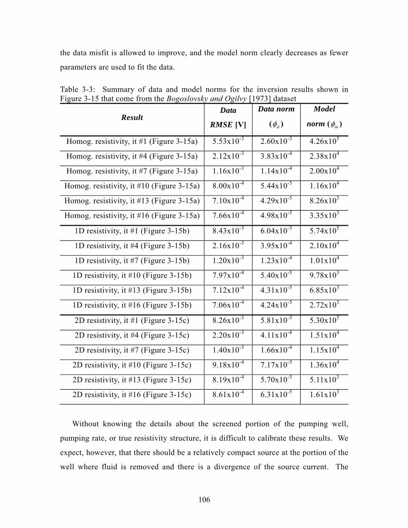
106

the data misfit is allowed to improve, and the model norm clearly decreases as fewer

parameters are used to fit the data.

Table 3-3: Summary of data and model norms for the inversion results shown in Figure 3-15 that come from the Bogoslovsky and Ogilvy [1973] dataset

Result Data

RMSE [V]

Data norm

( dφ )

Model

norm ( mφ )

Homog. resistivity, it #1 (Figure 3-15a) 5.53x10-3 2.60x10-3 4.26x105






1D resistivity, it #1 (Figure 3-15b) 8.43x10-3 6.04x10-3 5.74x105






2D resistivity, it #1 (Figure 3-15c) 8.26x10-3 5.81x10-3 5.30x105






Without knowing the details about the screened portion of the pumping well,

pumping rate, or true resistivity structure, it is difficult to calibrate these results. We

expect, however, that there should be a relatively compact source at the portion of the

well where fluid is removed and there is a divergence of the source current. The

107

deeper source solution using the 2D resistivity model for iterations 10-16 best repre-

sents pumping somewhere between the groundwater level of 17m at the well and well

depth of ~22m estimated from Figure 3-13. The sources for the homogeneous and 1D

resistivity models do not extend below the water table. This supports the argument

that a more realistic resistivity structure produces better source results, though moder-

ate differences in resistivity structure still produce similar images. In general, we are

successfully able to reconstruct the expected spatial distribution of SP sources from a

single surface profile.

These results can be compared with the current sources calculated by Darnet et al.

[2003] based on equation (3.26) and their hydraulic property estimates.

( )

2

3/ 2

02 2 2 20

ln /4

sgLQI

Q r rK r h

K

ρ

ππ

=⎛ ⎞

+⎜ ⎟⎝ ⎠

(3.26)

Here, ρ is the fluid density (kg·m-3), g is the gravitational acceleration (m·s-2), L is the

coupling coefficient (mV·S·MPa-1·m-1), Q is the pumping rate (m3·s-1), K is the hy-

draulic conductivity (m·s-1), r is the radial distance from the well (m), h0 (m) is the

water elevation at the well measured from a datum at 28m, and r0 (m) is the inner ra-

dius of the well. From their estimates of Q/K = 290m2, L = 0.8 mV·S·MPa-1·m-1, h0 =

11m, and r0 = 0.09m, the electrokinetic current source (Is) at r = r0 and r = 1m equals

1.5mA·m-3 and 0.002mA·m-3, respectively.

Equation (3.26) is derived from the Dupuit-Forchheimer formula, which is known

to be less accurate in the vicinity of the well where flow is no longer mostly horizon-

tal [Marsily, 1986, chapter 7]. Given this knowledge, as well as uncertainties in-

volved with the hydraulic properties of interest, we use 0.002mA·m-3 to 1.5mA·m-3 as

a rough estimate of the current source in the vicinity of the well. This compares fa-

vorably with the values taken from our source inversion results. The maximum am-

plitude for the current source at iteration 1 is approximately 0.04mA (Figure 3-15, top

row), which corresponds to 0.0025mA·m-3 given the 16m3 block size. At iteration 16

(Figure 3-15, bottom row), the current source amplitude is approximately 8mA, or

0.50mA·m-3. This correspondence with the results of Darnet et al. [2003] suggests

108

that our source inversion methods could also be used to make inferences about the

associated hydraulic properties.

Besides some uncertainty in the parameters used to compute the current source

estimate in equation (3.26), there are several other factors that can account for the

discrepancy between the inversion results and predicted values. First, recall from the

synthetic example that only approximately 20% of the true source amplitudes were

recovered. This is due to the limited data aperture, which cannot completely recover

the compact sources, and may be further influenced by noisy data. Second, we expect

that equation (3.26) will over-predict the current sources in the vicinity of the well

because the true piezometric head near the well lies above that predicted by the Du-

puit-Forchheimer formula [Marsily, 1986]. (i.e. the term in parenthesis in the de-

nominator of equation (3.26) is too small). Thus, we expect that the inverted current

source amplitudes will be an under-estimate of the true values, especially near the

well.

3.8 Discussion and conclusions

A robust method for 3D self-potential source inversion is presented that can provide

depth resolution from limited surface data. Resistivity structure and model geometry

are incorporated into the problem through use of the sensitivity kernel that is calcu-

lated using reciprocity. Methods for addressing the non-uniqueness and large sensi-

tivity variations are described that may also be useful in other potential-field inverse

problems. Spatial compactness is appropriate for SP sources, but the degree of com-

pactness will vary in different situations. The interpreter must therefore choose the

most appropriate class of solutions based on prior expectations about the distribution

of sources though, as previously stated, this study does not aim to characterize the

specific SP source mechanisms.

An important point that was not directly addressed in the previous examples is the

influence of the survey aperture. In all cases, the measured potential field was due to

sources located below the array of electrodes, and the amplitude of the potentials de-

109

cayed to near-background levels at the limits of the survey area. This is an ideal

situation, but is not always achieved in practice. That is, a portion of the self-

potential signal may come from sources that are laterally outside, but not far from, the

edges of the survey area. In this case, the sensitivity of the data to the source shape

and location is limited, and the source inversion results are therefore degraded accord-

ingly. For surveys with unknown source locations, it is therefore good practice to run

several synthetic models that use the actual survey geometry and various known

sources located outside the survey area. Inverting these datasets will give some feel

for the ability of the acquisition geometry to recover information outside the main

survey area. When acquiring field datasets, it is therefore desirable to extend the

measurement area so that the potential field returns to ‘background’ levels at the lim-

its of the survey.

Future work involves the incorporation of more complex model geometries and

development of efficient processing algorithms. One important step requires the defi-

nition of ‘convergence criteria’ that can be used to select from models with equal data

misfit based on prior information. The expected spatial statistics of the source distri-

bution, ideally determined from the relevant physics and chemistry of the coupling

phenomena, may provide useful information in this regard. Calculation of the sensi-

tivities can be time consuming for large models with many measurements (N forward

calculations), but can be accomplished efficiently by dividing the computations

among several parallel processors, which is another improvement we hope to incorpo-

rate. Finally, the results of the SP source inversion should be used to then estimate

the hydraulic, chemical, or thermal properties of interest. This is not a computation-

ally expensive task, but requires some knowledge about the forcing mechanism such

as the coupling coefficient structure and boundary conditions for the primary flow.

110

Figure 3-1: (A) Illustration of the non-quadratic term in the objective function for the compactness constraint defined in equation 4 for several values of β. These are com-pared with a traditional quadratic term (grey line). (B) The linearized version of the compactness term in the objective function, which is now a function of both β and a prior model estimate sj−1.

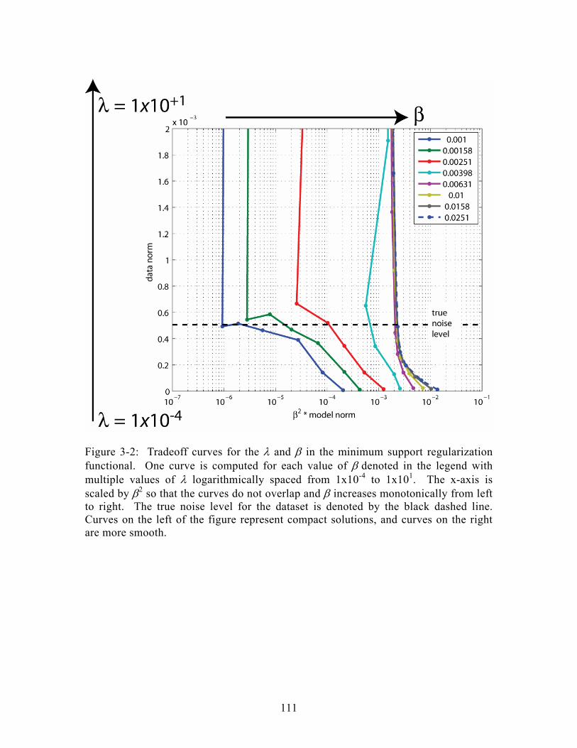
111

Figure 3-2: Tradeoff curves for the λ and β in the minimum support regularization functional. One curve is computed for each value of β denoted in the legend with multiple values of λ logarithmically spaced from 1x10-4 to 1x101. The x-axis is scaled by β2 so that the curves do not overlap and β increases monotonically from left to right. The true noise level for the dataset is denoted by the black dashed line. Curves on the left of the figure represent compact solutions, and curves on the right are more smooth.

112

Figure 3-3: Synthetic 2D source model (A) has a negative point source with magni-tude -3mA and dipping positive source with magnitude +1.5mA. Measurement loca-tions at the surface of the model are denoted by black triangles. (B) Noise-free data corresponding to the source model in a homogeneous resistivity structure.

113

Figure 3-4: Inversion results for the data in Figure 3-3b using traditional linear regu-larization techniques (equation (3.15)). (A) m =W I , (B) m = ∇W , (C) 2

m = ∇W . The true source locations are depicted by white asterisks.

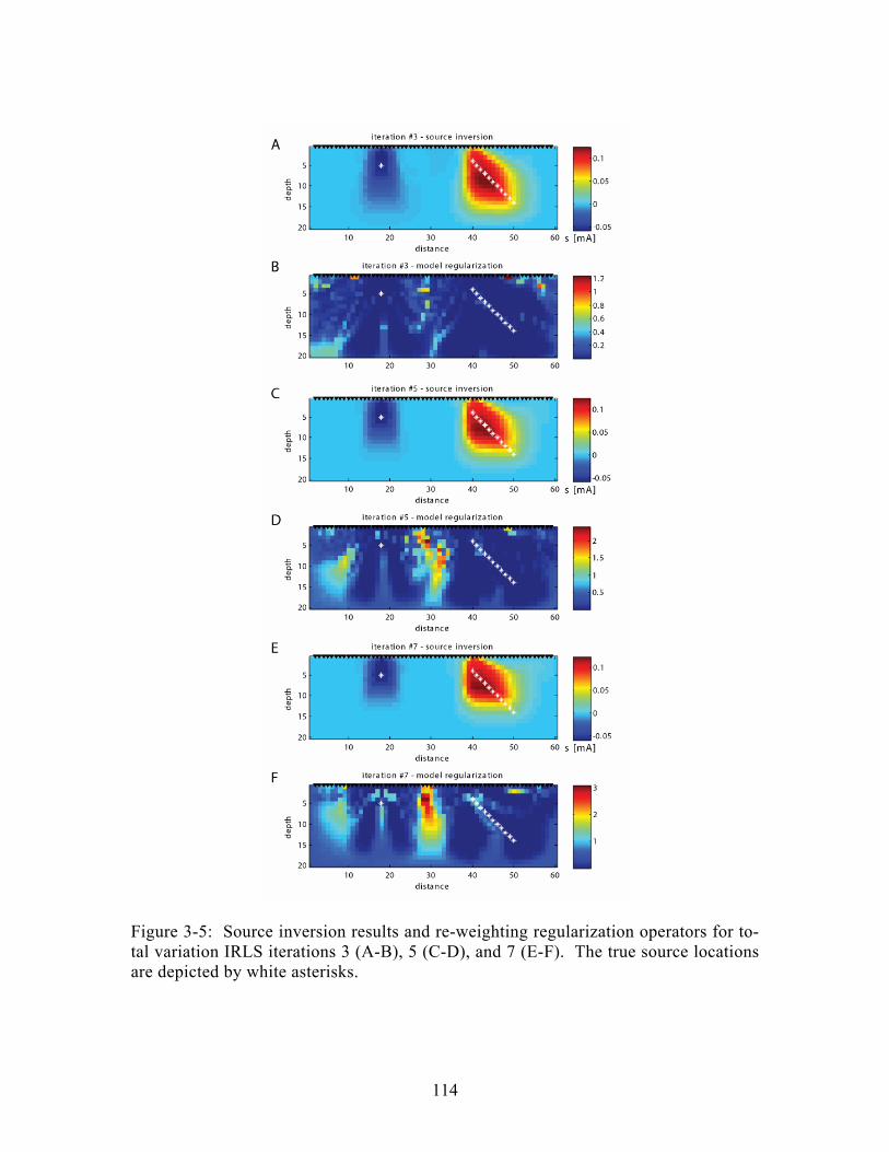
114

Figure 3-5: Source inversion results and re-weighting regularization operators for to-tal variation IRLS iterations 3 (A-B), 5 (C-D), and 7 (E-F). The true source locations are depicted by white asterisks.

115

Figure 3-6: Source inversion results and re-weighting regularization operators for compactness IRLS iterations 3 (A-B), 5 (C-D), and 7 (E-F). The true source locations are depicted by white asterisks.

116

Figure 3-7: Source inversion results an re-weighting regularization operators for compactness IRLS iterations 1 (A), 3(B-C), and 5 (D-E) when 10% zero-mean Gaus-sian noise is added to the data in Figure 3-3B. The general source locations are still captured, but the shape of the anomalies cannot be reconstructed due to the influence of noise.

117

Figure 3-8: Vertical slices through the initial 3D synthetic current source model at x=16 (top) and x=20 (bottom). Axes are labeled by node number, and the node spac-ing is 5m. True source amplitudes are ±10mA.

118

Figure 3-9: Synthetic SP data generated from the source model in Figure 3-8. Data are sampled at 60 random surface locations to simulate a typical SP survey.

119

Figure 3-10: A) Minimum length source solution along x = 16 (top) and x = 20 (bot-tom). The sources have been pulled to the surface measurement locations. B) Cumu-lative sensitivities (Λ) calculated from the sensitivity kernel (J) using equation (3.11) along the same two profiles. The very low sensitivities near the edges are because padding blocks are used with large node spacing so that the boundaries are far from the region of interest. C) Source solution using equation (3.14) that incorporates the sensitivity weighting term, which begins to include sources at depth.

120

Figure 3-11: Iterative weighting terms (top row) along x = 20 and source inversion results (bottom two rows) along x = 16 and x = 20 for iterations 1 (A), 4 (B), and 7 (C). The starting model corresponds to s0 = 0, therefore iteration #1 corresponds to the sensitivity weighted minimum norm solution. Note the different color scale for each iteration, where iteration 7 recovers approximately 20% of the true source ampli-tude.

121

Figure 3-12: Three synthetic examples that illustrate the effect of unknown resistivity structure on the source inversion results. The true resistivity structures (panels A, C, and E) are used to generate a synthetic dataset with a dipping source at the locations outlined in white. Each dataset is then inverted using a homogeneous 100 Ω·m model to produce the source inversion results shown on the right (panels B, D, and F).

122

Figure 3-13: Self-potential profile (top) in the vicinity of a pumping well (K-1, bot-tom). The water table elevation is estimated in the bottom part of the figure from pie-zometers in monitoring wells. Note the influence of infiltration from the surface drainage ditches near -70 and +110m on the self-potential signal. 85 SP measure-ments are discretized from the original figure [Bogoslovsky and Ogilvy, 1973].

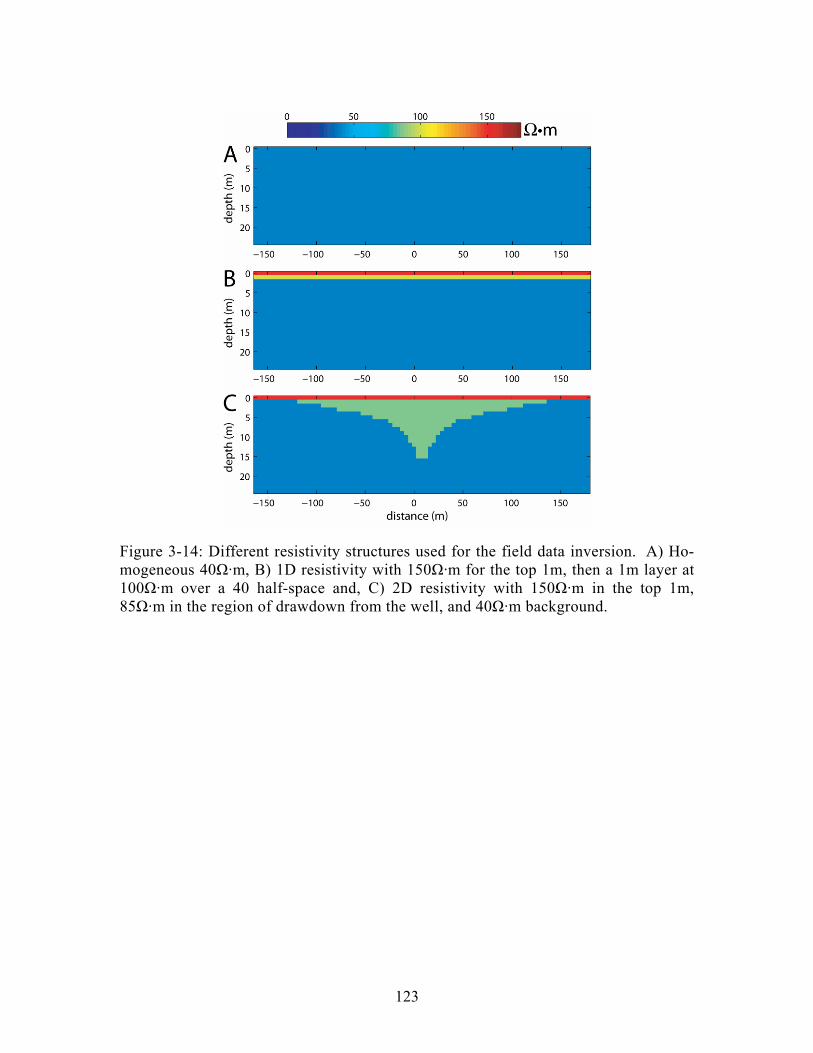
123

Figure 3-14: Different resistivity structures used for the field data inversion. A) Ho-mogeneous 40Ω·m, B) 1D resistivity with 150Ω·m for the top 1m, then a 1m layer at 100Ω·m over a 40 half-space and, C) 2D resistivity with 150Ω·m in the top 1m, 85Ω·m in the region of drawdown from the well, and 40Ω·m background.

124

Figure 3-15: Source estimates for the field data example corresponding to the homo-geneous resistivity (column A), 1D resistivity (column B), and 2D resistivity (column C). Increasing compactness, observed from top to bottom for each example, is due to the minimum support re-weighting. A smoothness constraint is enforced during the early iterations to remove the influence of noisy data, and is subsequently relaxed as the compact source solution becomes more stable. The location of the water table, pumping well, and drainage ditches are superimposed on the source images.

125

Figure 3-16: Data fit for three iterations of the compact source solution with the 1D resistivity structure. Note the rough fit for the first iteration, which has a strong smoothness constraint to avoid near surface artifacts due to the noisy data. This con-straint is relaxed at later iterations, which is evident by the improved data fit.

127

Chapter 4

Quantifying the effect of resistivity uncertainty on self-potential data analysis

4.1 Introduction

Self-potential signals result from the coupling between electric currents in the earth

and a primary forcing mechanism, which typically involves hydraulic, thermal, or

chemical gradients [e.g. Nourbehecht, 1963; Sill, 1983; Wurmstich, 1995]. The task

of self-potential interpretation is to make inferences about the primary forcing (or

source) mechanism from measurements of the electric potential field made remotely

from the source region, often at the surface of the earth. In general, the sources oc-

cupy a limited volume in the subsurface, and are located at an unknown distance from

the measurement locations. An analogous problem in the medical community in-

volves the electroencephalogram (EEG), where electrical potentials can be measured

on the scalp due to sources within the brain [e.g. Michel et al., 2004].

These problems are similar in that they are governed by the flow of electric cur-

rents in a conductive medium, albeit with different geometries, where the measured

potential field is used to characterize an unknown source mechanism. The measur-

able potential field is therefore a function of both the unknown sources and the resis-

tivity structure of the medium, which typically poorly known. In this chapter, I ad-

128

dress how imperfect knowledge of the earth resistivity structure influences self-

potential data interpretation. Similar studies have investigated the influence of skull

conductivity for the EEG problem [Pohlmeier et al., 1997], and have also included

influence of resistivity anisotropy [Marin et al., 1998; Wolters et al., 2006].

Numerous approaches have been developed to interpret self-potential measure-

ments using various forms of forward and inverse modeling [Fitterman and Corwin,

1982; Fournier, 1989; Birch, 1998; Shi, 1998; Gibert and Pessel, 2001; Sailhac and

Marquis, 2001; Revil et al., 2003a; Revil et al., 2004; Minsley et al., 2007]. This

work follows the technique of Minsley et al. [2007], as discussed in Chapter 3, where

the entire medium is discretized and a source distribution is determined by inverting

the self-potential measurements using an assumed resistivity structure within a least

squares framework. Even with the correct resistivity structure, this is an inherently

non-unique problem with multiple solutions that fit the data. We select a class of so-

lutions that are spatially compact by imposing model constraints in the inverse prob-

lem that satisfy this prior assumption about the source structure.

One component of error in the recovered source model is due to the assumptions

that must be made about the resistivity structure of the medium. Several studies in-

corporate information from a resistivity survey into the self-potential interpretation

[e.g. Yasukawa et al., 2003; Naudet et al., 2004; Revil et al., 2005], though in many

cases a simple homogeneous structure is assumed. In either situation, these imperfect

representations of the true earth structure will propagate as errors in the source inver-

sion, which we seek to understand and quantify.

4.2 Background

4.2.1 Self-potential sources

Self-potentials result from conduction currents in the earth that are generated by a

primary forcing mechanism, such as fluid flow, which provides a source current.

129

Thus, the total current density [A·m-2] in the earth is composed of a source current

( sj ) and a conduction current ( cj )

1( ) ( ) ( ) ( ) ( ) ( )s c sj j j j ρ ϕ−= + = + ∇x x x x x x , (4.1)

where ( )ρ x [Ω·m] represents the resistivity structure and ( )ϕ x [V] are the electric

potentials. The total current density must be divergence-free under the quasi-static

assumption, resulting in the familiar dc geoelectric governing equation (4.2), where

the forcing term on the right hand side [A·m-3] is related to the properties of the

source current.

( ) ( ) ( )1 ( )sj sρ ϕ−−∇ ⋅ ∇ = ∇ ⋅ =x x x x (4.2)

This is the same as equation (2.11), but is expressed in terms of the resistivity struc-

ture, which is more relevant to the discussion in this chapter.

The self-potential problem is often modeled in a two-step approach [Sill, 1983;

Sheffer et al., 2004]. First, the electrical source term on the right hand side of equa-

tion (4.2) is computed based on the physics of the appropriate source mechanism of

interest. Next, the electrical source term is used to calculate electrical potentials

throughout the model by solving equation (4.2). This chapter focuses primarily on the

second step, though some description of the source mechanism is also relevant to our

discussion.

Although the specific nature of the source current varies for different problems,

we adapt a general form for the source current [e.g. Ishido and Mizutani, 1981; Sill,

1983]

( ) ( ) ( )sj L ψ= ∇x x x , (4.3)

where ( )ψ x represents a potential (e.g. hydraulic, chemical, thermal) and ( )L x is the

coupling coefficient. An important point in the following discussion is that the cou-

pling coefficient, and therefore ( )s x , can be a function of resistivity. A common ex-

ample involves streaming potentials, where ( )ψ x represents hydraulic pressure and a

simplified form of the electrokinetic coupling coefficient [A·Pa-1·m-1] is given by

130

equation (4.4), which is also equivalent to equation (2.29) [e.g. Ishido and Mizutani,

1981; Morgan et al., 1989; Revil et al., 1999b].

fekL

εζρηρ

−= (4.4)

In the coupling coefficient, ε is the fluid dielectric constant [F·m-1], ζ is the zeta po-

tential [V], ρf is the fluid resistivity [Ω·m], η is the fluid viscosity [Pa·s], and ρ is the

bulk resistivity [Ω·m].

4.2.2 Description of the forward and inverse problems

Equation (4.2) is approximated using the transmission network approach [Madden

and Swift, 1969], which is discussed further in the context of the quasi-static geoelec-

tric problem by Zhang et al. [1995] and Shi [1998], and in Appendix A of this disser-

tation. A model is discretized into network nodes and impedance branches (Figure

A-1), where the impedances [Ω] are defined by the node spacing and model resistivi-

ties. This results in a linear system of equations (4.5) that is equivalent to finite ele-

ment or finite difference methods.

( ) =K ρ φ s (4.5)

This is the same as equation (3.3); the fact that K depends on the model resistivity is

highlighted here, as this is the main focus of the following discussion.

The impedance equations given by Zhang et al. [1995, equations 3a-c] are re-

peated here,

1 1( ) ( , , ) ( 1) ( 1, , )( ) ( ) ( ) ( )

1( ) ( , , 1) ( 1) ( 1, , 1)( ) ( 1) ( ) ( 1)

xx i i j k x i i j kRy j z k y j z k

x i i j k x i i j ky j z k y j z k

ρ ρ

ρ ρ

=∆ ∆ − −

+∆ ∆ ∆ ∆

+∆ − ∆ − − −

+∆ ∆ − ∆ ∆ −

, (4.6)

131

1 1( ) ( , , ) ( 1) ( , 1, )

( ) ( ) ( ) ( )1

( ) ( , , 1) ( 1) ( , 1, 1)( ) ( 1) ( ) ( 1)

yy j i j k y j i j kR

x i z k x i z k

y j i j k y i i j kx i z k x i z k

ρ ρ

ρ ρ

=∆ ∆ − −

+∆ ∆ ∆ ∆

+∆ − ∆ − − −

+∆ ∆ − ∆ ∆ −

, (4.7)

1 ( ) ( )( ) ( , , )z

x i y jR z k i j kρ

∆ ∆=

∆, (4.8)

where ∆x(i), ∆y(j), and ∆z(k) define the node spacing for the block with resistivity

ρ(i,j,k). The stiffness matrix, K, is banded and square symmetric, with a number of

rows equal to the number of nodes in the model. Entries along the nth row are deter-

mined by the L impedance branches that connect nodes m and n such that

1

1

1 connected to

0 not connected to

L

l nl

nmnm

n mR

K n mR

n m

=

⎧ ⎛ ⎞ =⎪ ⎜ ⎟⎝ ⎠⎪

⎪⎪ ⎛ ⎞= −⎨ ⎜ ⎟⎝ ⎠⎪

⎪⎪⎪⎩

∑

. (4.9)

In three dimensions, an interior node has 6L = impedance branches connected to it.

The forward problem of computing the measurable potential field is defined by

equation (4.10), which can be expressed as the inner product of a source term and the

Green’s function, Gϕ , which depends on the resistivity structure of the medium.

( ) ( ) ( ); ,G s dϕ ϕ ρ′ ′ ′= ∫x x x x xD

(4.10)

In discrete form, this involves solving equation (4.5) for ϕ, given K and s. Given

homogeneous boundary conditions, this is a well-posed problem because K is positive

definite symmetric.

The self-potential source inverse problem is stated in equation (4.11), where the

measured data, d, is a subset of the full potential field, ϕ.

1− = =PK s Pφ d (4.11)

132

P is a sparse matrix with a single ‘1’ in each row that selects the value of ϕ that corre-

sponds to the measurement locations associated with d. 1−K represents the discrete

form of the Green’s function in equation (4.10), though the inverse problem is limited

to a subset of the rows of 1−K selected by P due to the finite set of measurement loca-

tions. 1−PK is poorly conditioned because the number of measurements is typically

much smaller than the number of unknown model parameters, and equation (4.11)

cannot be solved directly for s. Instead, we find a source solution that minimizes a

joint measure of data misfit and a model regularization term, i.e.

( ) 2 2122

arg min d mλ−⎡ ⎤= − +⎢ ⎥⎣ ⎦ss W PK s d W s (4.12)

The solution of this problem is described in Chapter 3, where a particular nonlin-

ear form of Wm is chosen to select spatially compact solutions. In general, however,

Wm can incorporate any other form of prior information that is deemed appropriate.

Information about measurement errors can be included in the data weighting operator,

Wd, though we use d =W I throughout this chapter, which does not address the issue

of noisy data.

4.3 Deriving the effect of resistivity assumptions on the forward problem

Because the true earth resistivity is never known completely, some assumptions must

go into the formation of K. Information from a resistivity survey collected in con-

junction with the self-potential survey is very useful, but often unavailable, and is

never a perfect representation of the earth. Simple resistivity models based on prior

assumptions about the survey area are often used during self-potential interpretations.

It is therefore important to understand the impact of these assumptions on our ability

to interpret self-potential data.

Differentiating equation (4.5) with respect to a single resistivity, jρ , gives

133

j j jρ ρ ρ

∂ ∂ ∂+ =

∂ ∂ ∂K φ sφ K , (4.13)

which can be re-arranged to provide the sensitivity of the potentials to a perturbation

in a single resistivity value in (4.14) [e.g. Rodi, 1976].

1

j j jρ ρ ρ−

⎛ ⎞∂ ∂ ∂= −⎜ ⎟⎜ ⎟∂ ∂ ∂⎝ ⎠

φ s KK φ (4.14)

The elements of jρ∂ ∂K can be computed explicitly using equations (4.6) through

(4.9), where most values are zero because each resistivity cell contributes to a maxi-

mum of only nine impedance branches. The full sensitivity matrix for all of the dis-

cretized resistivity values is given in equation (4.15).

1 1

1

1

1 2

1

m

m

m m

m

ϕ ϕρ ρ

ρ ρ ρϕ ϕρ ρ

−

⎡ ⎤∂ ∂⎢ ⎥∂ ∂⎢ ⎥

⎛ ⎞⎢ ⎥ ⎡ ⎤∂ ∂ ∂ ∂ ∂= = −⎜ ⎟⎢ ⎥ ⎢ ⎥⎜ ⎟∂ ∂ ∂ ∂ ∂⎣ ⎦⎢ ⎥ ⎝ ⎠

⎢ ⎥∂ ∂⎢ ⎥

∂ ∂⎣ ⎦

φ s K K KK φ φ φρ ρ

(4.15)

The node potentials,ϕ, can be expanded in a Taylor series (4.16) for perturbations

to the resistivity structure.

( ) ( ) ( )2, ( , ) , Oδ δ δ+ = + ∂ +ρφ s ρ ρ φ s ρ φ s ρ ρ ρ (4.16)

Substituting equations (4.5) and (4.15) into equation (4.16) and ignoring the second

order term yields an expression for the measurable potentials as a function of the re-

sistivity perturbation (4.17).

( ) 1 1 1 1

1

,m

δ δρ ρ

− − − −⎛ ⎞⎡ ⎤∂ ∂ ∂+ = + −⎜ ⎟⎢ ⎥⎜ ⎟∂ ∂ ∂⎣ ⎦⎝ ⎠

s K Kφ s ρ ρ K s K K s K s ρρ

(4.17)

It is useful to consider a single measurement of the potential field,

( ),Ti iϕ δ= +a φ s ρ ρ (4.18)

134

where [ ]0 0 1 0 0Ti =a is a single row from P in equation (4.11)

with a ‘1’ in the column corresponding to the ith measurement location. Equation

(4.19) provides the complete expression for the ith potential measurement, which is a

function of the resistivity perturbations.

1 1 1T Ti i m i

m m

a aϕ δρ δρ

− − −⎡ ⎤∂ ∂= − +⎢ ⎥∂ ∂⎣ ⎦

∑ K sK I K s K ρρ

(4.19)

This equation provides useful insights into how resistivity uncertainties translate

into errors in the forward and inverse problems. The bracketed term in equation

(4.19) can be interpreted as a modification to the operator 1−K , with perturbations

arising due to the locations where 0iδρ ≠ . Alternatively, one can consider 1−K oper-

ating on three ‘source’ terms, as shown in equation (4.20).

[ ]1 1T Ti i i m

m m

a aϕ δρ δρ

− − ⎡ ⎤∂ ∂′ ′′= + + = − +⎢ ⎥∂ ∂⎣ ⎦∑ K sK s s s K s φ ρ

ρ (4.20)

It is important to note that s´ and s˝ are not physically real sources, but can be used

mathematically to correct for the erroneous resistivity assumptions. That is, the op-

eration of 1−K on s, s´, or s˝ results in a set of ‘potentials’ as defined by the forward

problem. An interesting point about s´ is that it can be expressed as a function of the

potential field due to s in the unperturbed part of the resistivity structure (i.e.

( )1−=φ K ρ s ).

The third term, s˝, is related to the fact that the self-potential source mechanism

discussed in section 4.2.1 can have a dependence on resistivity. If the fully coupled

problem is modeled by first determining s from equations (4.3) and (4.4) using an in-

correct resistivity assumption, the resulting electrical potentials will also be in error.

The sensitivity of the source term to the ith resistivity cell can be found from equa-

tions (4.2) and (4.3).

si i iρ ρ ρ

∂ ∂ ∂= ∇ ⋅ = ∇ ⋅ ∇

∂ ∂ ∂s Lj ψ (4.21)

135

Equation (4.21) has the same form as equation (4.2), with →φ ψ and 1iρ ρ− → ∂ ∂L ,

where iρ∂ ∂L has a single non-zero element that can be computed from equation

(4.4). This system can be discretized in the same fashion as equation (4.5), such that

ii iρ ρ

⎛ ⎞∂ ∂=⎜ ⎟∂ ∂⎝ ⎠

L sM ψ , (4.22)

where i→K M and iρ→ ∂ ∂s s . The elements of iM [A·Pa-1·Ω-1·m-1] can be deter-

mined using equations (4.6) through (4.9) by substituting iρ∂ ∂L for 1ρ − . iM is very

sparse because iρ∂ ∂L has only one non-zero element; therefore a maximum of nine

nodes (or rows of iM ) have a contribution from the non-zero value. The complete

expression for s˝ in equation (4.20) is therefore

11

mm

δρ ρ

⎡ ⎤⎛ ⎞⎛ ⎞∂ ∂′′ = ⎢ ⎥⎜ ⎟⎜ ⎟∂ ∂⎢ ⎥⎝ ⎠ ⎝ ⎠⎣ ⎦

L Ls M ψ M ψ ρ . (4.23)

Because 1−K is symmetric,

( )1 1 TT Ti i i

− −= =a K K a u . (4.24)

Equation (4.24) shows that the expression 1Ti

−a K found in equations (4.19) and (4.20)

is equal to a vector of ‘pseudo-potentials’ ui (i.e. the adjoint field), which are com-

puted by solving a single forward problem with a unit source at the ith measurement

location. Equation (4.20) can therefore be simplified as

[ ] 1T Ti i i m

m m

ϕ δρ δρ

−⎡ ⎤∂ ∂′ ′′= + + = − +⎢ ⎥∂ ∂⎣ ⎦∑ K su s s s u s K s ρ

ρ. (4.25)

From equation (4.25), we see that the potential at the ith station is described by

the interaction of the adjoint field computed using the assumed resistivity structure

with three ‘source’ terms. s is the true source distribution, s´ consists of the forward

potential field in the assumed resistivity structure ( 1−K s ) times the scaled sum of sen-

sitivities of the forward operator (K) to the resistivity structure, and s˝ is composed of

136

the resistivity perturbations times the sensitivities of the source mechanism to the re-

sistivity structure.

Several useful inferences can be made regarding the influence of resistivity uncer-

tainties on measurable potentials from equation (4.25). The second term, Ti ′u s , sug-

gests that the resistivity perturbation will have the greatest effect when (1) the pertur-

bation is near the receiver ( Tiu is large), (2) the perturbation is near the source ( 1−K s

is large), (3) the magnitude of mδρ is large, or (4) the spatial extent where 0mδρ ≠ is

large. The third term, Ti ′′u s , has the greatest effect when (1) the resistivity perturba-

tion is located in the source region (because ∂ ∂s ρ is diagonal) and (2) the magnitude

of mδρ is large. These insights confirm more qualitative or intuitive expectations re-

garding the influence of unknown resistivity structure [e.g. Marin et al., 1998].

4.4 The influence of resistivity uncertainty on self-potential source inversion

In this section, we illustrate how imperfect knowledge of the resistivity structure in-

fluences self-potential source inversion using several synthetic examples. The inverse

method, discussed in Chapter 3, seeks to find a distributed electrical source model ac-

cording to equation (4.12) that explains the measured data in addition to satisfying a

constraint that the sources should be spatially compact. Model constraints are neces-

sary to overcome the inherent non-uniqueness of the source inverse problem, though

various forms of prior information other than compactness may be used. In the fol-

lowing examples, compactness is an appropriate choice because the synthetic model

consists of a point source.

A three-dimensional synthetic model is generated with [ ] [ ], , 71,71, 25nx ny nz = ,

where the node spacing in all directions is 1m (Figure 4-1a). Boundary nodes with

larger spacing are utilized at the sides and bottom of the model to satisfy the Dirichlet

boundary conditions far away from the source region. The true source model is a

137

positive point source with magnitude 10mA at [ ] [ ], , 36 ,36 , 6x y z m m m= − . That is, we

define the electrical source explicitly for these examples, which removes the effects

of resistivity on the source magnitude and the resulting potential field due to s˝ in

equation (4.25). A dense grid of 337 surface measurement locations is used to simu-

late a surface self-potential dataset (black dots in Figure 4-1a). The simple source

model and dense set of noise-free measurements is utilized to highlight only the ef-

fects of perturbing the resistivity structure.

Figure 4-1b shows a mesh-plot of the potential field computed from equation (4.5)

using the true source model in a homogeneous resistivity structure of 100Ω·m. The

potential field is symmetric over the point source, with maximum amplitude approxi-

mately 32mV. Figure 4-1c shows a slice of the source inversion results along x =

36m, highlighted by the white line in Figure 4-1b, where the correct homogeneous

resistivity structure is assumed. Note that the inversion is able to properly locate the

point source in the subsurface, though the source amplitude is approximately 60% of

the true value. This is likely due to the fact that surface measurements alone do not

provide a large enough aperture to completely reconstruct the source.

Next, we show several examples where the synthetic data are computed using the

same point source model, but different “true” resistivity structures. The source inver-

sion is then carried out by assuming an incorrect 100Ω·m homogeneous resistivity

structure. Noise-free data are used for all of the synthetic examples in order to high-

light only the effects of the incorrect resistivity assumptions. Table 4-1 summarizes

the data and model norms for all of the following inversion results. Note that the data

RMS error is allowed to be small (< 1mV) for all of the examples due to the lack of

measurement noise.

4.4.1 1D resistivity structures

Three different examples are investigated where the true resistivity structure consists

of a layer of either 10Ω·m or 1000Ω·m embedded within a background resistivity of

100Ω·m. The anomalous resistivity layer is above the source in the first case, below

138

the source in the second case, and at the same depth as the source in the third case.

The forward data computed with these true resistivity structures are then inverted by

constructing 1−K with a homogeneous 100Ω·m resistivity assumption.

The first example, shown in Figure 4-2, illustrates the effect of the anomalous re-

sistivity in a thin near-surface layer. Figure 4-2a-b show the true model for the con-

ductive and resistive near surface layers, with a mesh-plot of the potential fields that

would be recorded at the stations indicated on the surface of the model. Figure 4-2c

displays the potentials along x = 36m, denoted by the white lines in Figure 4-2a-b.

The potentials for the homogeneous resistivity case (Figure 4-1) are shown in black,

for the conductive near-surface layer in blue, and for the resistive near-surface layer

in red. As expected, there is a clear influence of the near-surface resistivity on the

shape and amplitude of the recorded potentials.

Inversion of these potential fields with the incorrect resistivity structure is there-

fore unable to recover the true point source, which is illustrated in Figure 4-2d-e. In

the case of the conductive near-surface layer, the potential field is broadened and re-

duced in amplitude due to the pseudo-sources, s´. The net effect can be explained by

the source distribution in Figure 4-2d, which is deeper than the true source in order to

fit the broader potential field. In Figure 4-2e, the recovered source is wider, and

slightly too shallow, than the true point source.

Figure 4-3 illustrates the same steps as Figure 4-2, but for the second case where

the resistivity perturbations are in a half-space below a 100Ω·m layer that contains the

source. The influence of the resistivity structure on the simulated potentials can be

seen in Figure 4-3a-c. Again, the amplitude of the self-potential anomaly is smaller

for the conductive case than for the resistive one, but the shapes of the potential fields

are also different. In Figure 4-2, the potential field for the resistive case is the “sharp-

est”- that is, they decay more rapidly from the peak value. In Figure 4-3, however,

the potentials for the conductive case decay most rapidly. This results in a shallow

recovered source for the conductive case (Figure 4-3d) and a deeper recovered source

for the resistive case (Figure 4-3e).

139

It is interesting to note that the source solution for the near-surface conductive

layer (Figure 4-2d) is similar to the solution for the resistive half-space (Figure 4-3e),

and the resistive near-surface layer solution (Figure 4-2e) is similar to the conductive

half-space solution (Figure 4-3d). This is due to the fact that the resistivity contrast

between layers is the same: 1 2 0.1ρ ρ = for the first two cases, and 1 2 10ρ ρ = for the

second two cases. The corresponding solutions are not exactly the same, however,

because of the differences in layer thickness.

A third case, where the anomalous resistivity consists of a thin layer at the same

depth as the source, is shown in Figure 4-4. Again, the simulated potentials for the

conductive layer case are significantly reduced, and decay more slowly than the case

with the resistive layer, as seen in Figure 4-4a-c. The source inversion using a homo-

geneous resistivity assumption therefore recovers a source that is too deep for the case

where the data are simulated using a conductive layer (Figure 4-4d). For the case

with the resistive layer, the inverted source model cannot be collapsed to a point, but

occupies a small volume at the correct depth.


Next, we examine the influence of lateral resistivity heterogeneities on the self-

potential source inversion. The examples in Figure 4-5a-b consist of either a conduc-

tive or resistive near-surface layer that covers approximately half of the model,

though it does not extend all the way over the source location. Laterally varying near-

surface heterogeneity can be common in self-potential surveys that traverse varying

soil types or saturation conditions. The potentials along x = 36m are no longer sym-

metric, as can be seen in Figure 4-5c. On any line parallel to the resistivity contrast

(constant y), however, the potentials are symmetric. This highlights the importance of

collecting data in two-dimensions when lateral resistivity heterogeneity is present.

It is clear from Figure 4-5c that the potentials computed from the model with the

resistive layer (red line) are more similar to the homogeneous case (black line) than

those computed from the model with the conductive layer (blue line). This difference

140

is manifested as a greater error in the source inversion for the conductive layer case

when a homogeneous resistivity structure is assumed. The inverted source for this

case is distorted both laterally and vertically, and appears as a dipping feature in

Figure 4-5d. In contrast, the source is only slightly distorted and mis-located for the

case with the resistive near-surface heterogeneity, as seen in Figure 4-5e.

A second laterally heterogeneous example is shown in Figure 4-6, where the resis-

tivity heterogeneity covers approximately half of the model, but does not extend all

the way to the surface. The source is located in the background 100Ω·m material,

several meters away from the contrast in resistivity. As with the previous case, the

forward-modeled potentials are no longer symmetric along x = 36m due to the 2d re-

sistivity structure (Figure 4-6c). The results of the source inversion using the incor-

rect (homogeneous 100Ω·m) resistivity structure are shown in Figure 4-6d-e. Again,

the case with the more conductive region appears as a dipping source, offset slightly

from the true source location. For the more resistive case, the recovered source is

generally in the correct location, but has a distorted and blurred shape.


Figure 4-7a-b illustrate slightly more complicated resistivity models that have both

conductive and resistive regions embedded within a 100Ω·m half-space, and the cor-

responding forward-modeled potential fields. Each case has a shallow trench that is

8m wide crossing the entire model and a 10m wide block that is perpendicular to, and

extends to within 15m of, the trench. The resulting potential fields are somewhat

more irregular (Figure 4-7c), and are no longer symmetric about any survey line in

the x- or y-directions. The corresponding source inversions using a homogeneous re-

sistivity assumption exhibit both mis-location and distortion of the source structure.

In both cases, the sources are smeared out in the direction of the more resistive por-

tion of the true resistivity model. Also, the overall mis-location for the case with the

more resistive trench (Figure 4-7b,e) is not as great as the case with the more conduc-

tive trench (Figure 4-7a,d).

141

A more realistic example is presented in Figure 4-8, where the true resistivity

structure is a spatially correlated random variable with a lognormal distribution. The

range of resistivity values is approximately the same as the previous examples (~10 to

1000Ω·m). In Figure 4-8a, the entire model has a random distribution with a mean

value of 183Ω·m; whereas in Figure 4-8b, the heterogeneity below the near-surface is

replaced by a constant half-space with resistivity equal to 183Ω·m. Comparing these

two cases helps to illustrate the relative importance of the near-surface resistivity

compared with subsurface resistivity variations.

The simulated self-potential data for these resistivity models is shown in Figure

4-8a-c. One notable feature is that the potential fields are smooth compared with the

other examples that contain near-surface lateral heterogeneity (Figure 4-5 and Figure

4-7) due to the fact that the resistivity contrast is less sharp. Also, while there is some

difference in the synthetic data generated from the fully heterogeneous (Figure 4-8a)

and near-surface heterogeneous (Figure 4-8b) structures, they have a very similar

shape, which is evident in Figure 4-8c. This is consistent with the example in Figure

4-3, where differences in the lower half-space result in similarly shaped potential

fields that are offset in amplitude. The source inversion results for these examples

using a homogeneous resistivity assumption are similar (Figure 4-8d-e), though the

case with the constant half-space is slightly better due to the fact that there are fewer

locations where the homogeneous assumption is incorrect. This also supports the ar-

guments in section 4.3 that suggest source inversion errors are greater when the resis-

tivity errors are near the receiver locations, or when a large volume of resistivity is

incorrectly estimated.

4.4.4 Partially known resistivity structure

Finally, we consider the case where the heterogeneous resistivity structure is partially

known, which may be the case when self-potential and resistivity surveys are carried

out in the same area. The simulated self-potential data from the forward model in

Figure 4-8a are inverted with smoothed estimates of the true resistivity structure,

142

shown in Figure 4-9. In Figure 4-9a, an average 2D resistivity structure ( ( ),y zρ ρ= )

is used as an input for the source inversion, which might be obtained from a 2D resis-

tivity survey. The corresponding source solution is shown in Figure 4-9b. Next, a

blurred 3D version of the true resistivity structure (Figure 4-9c) is used as an input for

the self-potential source inversion, with results shown in Figure 4-9d. While there is

still some degree of distortion and mis-location of the source results using a partially

known resistivity structure, both results in Figure 4-9 show an improvement over the

case where a homogeneous resistivity structure is used (Figure 4-8d).

Table 4-1: Summary of data and model norms for the synthetic inversion results based on Figure 4-1

Result Data RMSE

[V]

Data norm

( dφ )

Model norm

( mφ )

1D resistivity (Figure 4-2a,d) 2.57x10-4 2.21x10-5 4.80x105

1D resistivity (Figure 4-2b,e) 2.10x10-5 1.49x10-7 2.69x105













Partial resistivity, 2D (Figure 4-9a,b) 7.39x10-4 1.83x10-4 1.07x106

Partial resistivity, 3D (Figure 4-9c,d) 3.79x10-4 4.84x10-5 2.28x106

143

4.5 Conclusions

We have demonstrated the influence of resistivity structure on the interpretation of

self-potential data, particularly in relation to self-potential source inversion. Based on

the analytic description of forward-modeled electric potentials and their sensitivity to

uncertainties in the resistivity of the medium discussed in section 4.3, we quantify the

cases where resistivity uncertainty is most important: (1) The resistivity uncertainty is

near the receiver locations, (2) the resistivity uncertainty is near the source locations,

(3) the self-potential coupling mechanism is strongly dependent on the resistivity, (4)

the magnitude of the resistivity uncertainty is large, or (5) the size of the region where

the resistivity assumption is incorrect is large. A combination of any of these cases

clearly enhances the effect on the measured potentials.

Synthetic examples help to illustrate the effect of resistivity uncertainty on the

self-potential source inversion problem. Mis-locations in the inverted sources for the

1D resistivity models are generally in the vertical direction, though sources can also

be smeared laterally somewhat. For the 2D and 3D resistivity examples, the inverted

sources can be mis-located both laterally and vertically, and can be distorted in shape.

These results provide useful insights into the types of errors that can be expected

when interpreting self-potential data with imperfect knowledge of the resistivity

structure. It is important to consider these errors in order to avoid misinterpreting

features in the data that are due to unaccounted for resistivity, rather than actual self-

potential source processes. We therefore promote the use of combined resistivity and

self-potential surveys where possible, as the resistivity information can be useful to

self-potential interpretation, and provides complementary information regarding sub-

surface structure.

144

Figure 4-1: a) Synthetic point source model with 337 surface measurement locations, b) potential field computed from the point source in a homogeneous 100Ω·m resistiv-ity structure, c) 2d slice of the inverted source model along x = 36m, denoted by the white line in b), assuming the correct resistivity structure. The inversion successfully recovers the true location of the point source, though the amplitude is slightly reduced

145

Figure 4-2: Synthetic models with a conductive (a) and resistive (b) near-surface layer over a 100Ω·m half-space, and a mesh-plot of the potentials computed at the measurement locations due to the point source in Figure 4-1. (c) Comparison of the poten-tials along x = 36m for the conductive near-surface layer (blue line), the resistive near-surface layer (red line), and the homoge-neous model (black line). (d,e) Source inversion results assuming a homogeneous resistivity structure for the data computed in (a) and (b), respectively. For reference, the white star represents the true source location, and the black dashed line denotes the location of the resistivity contrast in the forward model.

146

Figure 4-3: Synthetic models with a conductive (a) and resistive (b) half-space below a 100Ω·m layer, and a mesh-plot of the potentials computed at the measurement locations due to the point source in Figure 4-1. (c) Comparison of the potentials along x = 36m for the conductive half-space (blue line), the resistive half-space (red line), and the homogeneous model (black line). (d,e) Source inversion results assuming a homogeneous resistivity structure for the data computed in (a) and (b), respectively. For reference, the white star represents the true source location, and the black dashed line denotes the location of the resistivity contrast in the forward model.

147

Figure 4-4: Synthetic models with a conductive (a) and resistive (b) layer within a 100Ω·m half-space, and a mesh-plot of the potentials computed at the measurement locations due to the point source in Figure 4-1. (c) Comparison of the potentials along x = 36m for the conductive layer (blue line), the resistive layer (red line), and the homogeneous model (black line). (d,e) Source inversion results assuming a homogeneous resistivity structure for the data computed in (a) and (b), respectively. For reference, the white star represents the true source location, and the black dashed line denotes the location of the resistivity contrast in the forward model.

148

Figure 4-5: Synthetic models with a conductive (a) and resistive (b) near-surface layer that extends partially over a 100Ω·m half-space, and a mesh-plot of the potentials computed at the measurement locations due to the point source in Figure 4-1. (c) Comparison of the potentials along x = 36m for the conductive layer (blue line), the resistive layer (red line), and the homogene-ous model (black line). (d,e) Source inversion results assuming a homogeneous resistivity structure for the data computed in (a) and (b), respectively. For reference, the white star represents the true source location, and the black dashed line denotes the loca-tion of the resistivity contrast in the forward model.

149

Figure 4-6: Synthetic models with a conductive (a) and resistive (b) region covering approximately half of the subsurface por-tion of the model, and a mesh-plot of the potentials computed at the measurement locations due to the point source in Figure 4-1. (c) Comparison of the potentials along x = 36m for the conductive region (blue line), the resistive region (red line), and the ho-mogeneous model (black line). (d,e) Source inversion results assuming a homogeneous resistivity structure for the data com-puted in (a) and (b), respectively. For reference, the white star represents the true source location, and the black dashed line de-notes the location of the resistivity contrast in the forward model.

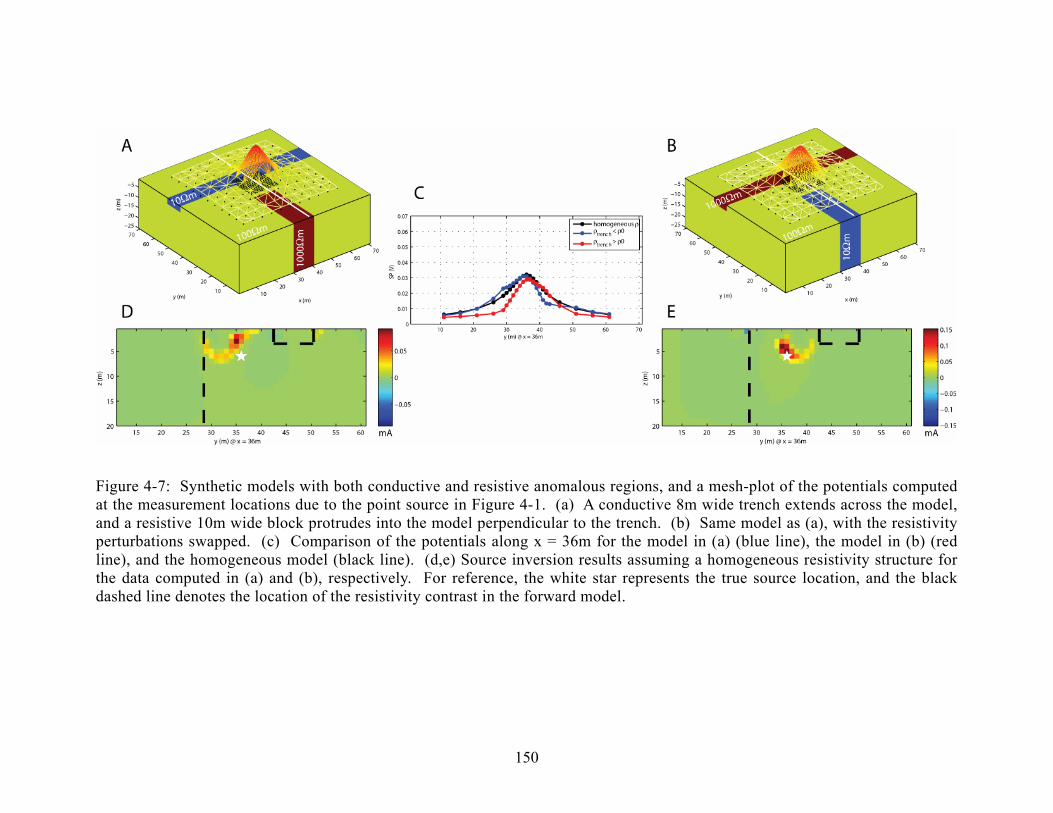
150

Figure 4-7: Synthetic models with both conductive and resistive anomalous regions, and a mesh-plot of the potentials computed at the measurement locations due to the point source in Figure 4-1. (a) A conductive 8m wide trench extends across the model, and a resistive 10m wide block protrudes into the model perpendicular to the trench. (b) Same model as (a), with the resistivity perturbations swapped. (c) Comparison of the potentials along x = 36m for the model in (a) (blue line), the model in (b) (red line), and the homogeneous model (black line). (d,e) Source inversion results assuming a homogeneous resistivity structure for the data computed in (a) and (b), respectively. For reference, the white star represents the true source location, and the black dashed line denotes the location of the resistivity contrast in the forward model.

151

Figure 4-8. Synthetic models with a spatially correlated lognormal resistivity distribution (a) throughout the entire model, and (b) within a near-surface layer, displayed with a mesh-plot of the potentials computed at the measurement locations due to the point source in Figure 4-1. (c) Comparison of the potentials along x = 36m for the model in (a) (blue line), the model in (b) (red line), and the homogeneous model (black line). (d,e) Source inversion results assuming a homogeneous resistivity structure for the data computed in (a) and (b), respectively. For reference, the white star represents the true source location, and the black dashed line denotes the location of the resistivity contrast in the forward model.

152

Figure 4-9. Smooth 2D (a) and 3D (c) versions of the true resistivity structure in Figure 4-8a used as input to the self-potential source inversion with the simulated data from Figure 4-8a. (b) The source inversion result using the 2D resistivity provides a more compact solution than Figure 4-8d, but the sources are still somewhat mis-located. (d) The use of a smooth 3D resistivity model better estimates the source depth, though there is still some lateral distortion.

154

Chapter 5

Three dimensional self-potential inversion for DNAPL contaminant detection at the Savannah River Site, South Carolina

5.1 Introduction

Chlorinated organic solvents, part of a larger group of chemicals referred to as Dense

Non-Aqueous Phase Liquids (DNAPLs), represent a significant portion of the world’s

groundwater contamination problem because of their extensive use during the past

fifty years. These chemicals can persist in the ground for a long time because of their

physical and chemical properties [Pankow and Cherry, 1996]. Combined with very

low maximum contaminant levels (MCLs) in water, which range from approximately

5-200 µg/L [Ajo-Franklin et al., 2005], these contaminants represent a long-term

groundwater hazard. Remediation of sites contaminated with these chemicals there-

fore remains an important issue today. The goal of this investigation is to characterize

underground contaminant distributions using minimally invasive geophysical meth-

ods, particularly self-potential, in order to improve site remediation efficiency.

There is growing interest in the use of geophysical methods for environmental

monitoring [Greenhouse et al., 1993; Daily and Ramirez, 1995; Lendvay et al., 1998;

Atekwana et al., 2000; Atekwana et al., 2004; Chambers et al., 2004; Mota et al.,

155

2004; Ajo-Franklin et al., 2005], and there have been several recent efforts to relate

self-potential measurements to subsurface contaminants [Perry et al., 1996; Vichabian

et al., 1999; Naudet et al., 2003; Naudet et al., 2004]. Self-potential is a general term

that describes spontaneously occurring electrical potentials caused by electrothermal,

electrokinetic (often called streaming potentials), or electrochemical coupling effects.

This method promises to be an effective tool for site characterization and monitoring

because it is sensitive to in-situ subsurface and contaminant chemistry, though bacte-

ria may also play an important role in the mediation of the redox processes that gen-

erate a self-potential signal [Atekwana et al., 2004; Naudet and Revil, 2005].

As with other potential-field methods, interpretation of SP data is inherently non-

unique [Blakely, 1995], and this is enhanced by the limited set of measurement loca-

tions often available within the volume of interest. In this investigation, a 3D array of

surface and borehole measurements is employed to provide greater data coverage. A

three-dimensional inversion algorithm is utilized to determine a self-potential current

source model that relates the measurements to the spatial distribution of contaminants.

Determination of the SP sources is an important step in relating the measured data to

physical properties of interest, and is relevant to other exploration and engineering

applications besides contaminant detection. The SP source inversion method used

here continues from the work of Shi [1998], which is also similar to electroencepha-

lographic imaging methods used in the medical community [e.g. Michel et al., 2004

and references within].

This procedure is employed at the A-14 outfall at the Savannah River Site (SRS),

a location with significant DNAPL contamination. During a 2001 field survey at the

SRS [Morgan, 2001], two SP transects were taken in the vicinity of the A-14 outfall.

Surface anomaly locations were qualitatively correlated with elevated DNAPL con-

centrations taken from several well measurements (Figure 5-1). While one should not

expect perfect correlation between surface self-potentials and elevated concentrations

at depth, the 2001 SP results justified a more thorough survey for the 2003 field ex-

periment, including a more rigorous analysis of the data. DNAPL concentration data

taken from several ground truth wells helps measure the success of this method,

156

though measurement of other environmental parameters (i.e. oxygen content, bacterial

presence, redox potential, organic nutrients) that may also contribute to the SP signal

is needed to make a more conclusive argument.

5.2 Background

5.2.1 A-14 Outfall

The A-14 outfall is located on the northwest side of the SRS (Figure 5-2). The outfall

is a surface discharge point of a process sewer system that serves the “A/M” area at

the SRS and feeds a tributary to Tims Branch, which ultimately leads to the Savannah

River along the border with Georgia. Various wastes from the fabrication facilities in

this area were released into the sewer system from 1952 until 1981, when it was real-

ized that DNAPLs were contaminating the groundwater below the settling basin just

south of the outfall.

Three varieties of chlorinated solvents were used as degreasers in the M-area, all

of which are classified as DNAPLs: tetrachloroethylene (PCE), trichloroethylene

(TCE), and trichloroethane (TCA). It is estimated that more than 600,000 kilograms

of these solvents were released to the A-14 outfall [Jackson et al., 1999]. Discharge

of chlorinated solvents at the A-14 outfall during a 30 year period resulted in exten-

sive vadose zone contamination. DNAPLs, being denser than water, generally mi-

grate downwards towards the water table, but are also influenced by subsurface struc-

ture, variations in hydraulic conductivity, capillary forces, microbial activity, and re-

cent remediation efforts.

The vadose zone beneath the “A/M” area extends approximately 40m below

ground surface, and is the primary area of interest for this study. Within this zone,

there are interbedded layers of sand, silt, and clay. The clays are not very thick or lat-

erally extensive, but tend to play a large role in the movement and distribution of

DNAPLs [Jackson et al., 1999; Parker et al., 2003]. There are varying reports on the

details of this structure, but there is general agreement that the vadose zone consists

of three or four distinct clay layers. In the vadose zone, a significant amount of resid-

157

ual DNAPL can be trapped in the pore space due to capillary forces. Subsurface het-

erogeneity therefore results in very complicated and difficult to predict contaminant

distributions at the A-14 outfall.

5.2.2 Contaminants as self-potential sources

The primary source of a self-potential signal at the A-14 outfall is proposed to be

electrochemical in nature. This is based on the limited 2001 data and little expected

influence from thermal or hydraulic gradients in the relatively small survey area,

though there may be some influence (several mV) from fluid flow in the vadose zone

[e.g. Guichet et al., 2003; Darnet and Marquis, 2004]. Naudet et al. [2004] ascribe

the self-potential signals to large scale redox zonation due to the influence of con-

taminants “in a natural geobattery process in which biofilms could play an important

role”. These geobatteries, which are associated with redox potential gradients, may

therefore be good indicators of DNAPL presence.

Electrochemical sources can be attributed to several phenomena, more than one of

which may be occurring at a given site [e.g. Kulessa et al., 2003]. A source current,

discussed in further detail in section 2.1.3, is generated as the contaminant is biode-

graded through microbially mediated redox reactions. These redox processes may

involve several intermediate compounds and electron transport chain components be-

fore the terminal electron acceptor is reduced [Lovley et al., 1994]. The source cur-

rent, embedded in the conductive earth structure, must be balanced by an external cur-

rent that flows throughout the earth according to the requirement that the total electric

current density is divergence-free. This results in a remote source term for the self-

potential signal that is measured at the earth surface. This system is analogous to the

corrosion of two metals in a short-circuited energy-producing cell described by Bock-

ris and Reddy [2000, chapter 12]. Another common electrochemical source mecha-

nism is the diffusion of ions due to a concentration gradient between two regions.

The source current due to diffusion is balanced by a current that flows throughout the

earth conductivity structure, again such that the total current density is divergence

free.

158

The three varieties of chlorinated solvents of concern at the A-14 outfall (PCE,

TCE, and TCA), consist of two carbon atoms that are each attached to a number of

chlorine and hydrogen atoms, shown in the shaded boxes in Figure 5-3. Halogenated

compounds tend to be relatively oxidized, increasingly so with the number of chlorine

atoms attached to the molecule [Vogel et al., 1987]. These chemicals can therefore

act as electron acceptors, and are reduced during reductive dechlorination. Several

pathways for the half-reactions involving the reductive dechlorination of the DNAPLs

found at the SRS are shown in Figure 5-3. This process is typically (though not ex-

clusively) biologically mediated, and occurs primarily in more reducing anaerobic en-

vironments where the chlorinated solvent becomes the primary electron acceptor

[Chen et al., 1996; Magnuson et al., 1998; Wiedemeier et al., 1999; Schwarzenbach et

al., 2003]. The presence of cis-DCE, one of the daughter products during reductive

dechlorination, at the A-14 outfall is evidence that this form of degradation has likely

taken place.

Another mechanism for the degradation of chlorinated solvents is cometabolism.

This process can involve the oxidation or reduction of contaminants in aerobic or an-

aerobic environments where microorganisms derive carbon and energy from metabo-

lism of a primary substrate, and the chlorinated solvent is degraded fortuitously

[Wiedemeier et al., 1999]. PCE is not known to undergo cometabolic degradation, as

it is limited to less oxidized chlorinated solvents with one or more hydrogen atoms

[Kao et al., 2003].

There is evidence that DNAPLs may be degraded by either of these methods in

different locations at the same field site. A recent field investigation at the A-14 out-

fall [Powers et al., 2003] suggests that microbial populations were capable of come-

tabolizing TCE in the generally aerobic conditions, but vadose zone heterogeneity

also provides localized anaerobic environments where reductive dechlorination takes

place. In general, degradation of chlorinated solvents results in a long-term decrease

of the redox potential, though the more chlorinated compounds may not degrade sig-

nificantly unless the conditions become more reducing [Wiedemeier et al., 1999].

159

Extended contaminant presence and degradation will therefore tend to be associ-

ated with zones of lower redox potential, with the exception of PCE contamination in

an aerobic area that does not degrade because oxygen remains the preferential elec-

tron acceptor. Redox gradients generated by these various reactions provide the

source of the SP signal. It is important to note however, that it is not only contami-

nant presence, but also factors such as microbial presence, oxygen content, and or-

ganic material that will determine the redox state of the subsurface.

5.3 Electrode and survey design

5.3.1 Electrode design

It is standard practice to use non-polarizing porous-pot electrodes (typically Ag-AgCl,

Cu-CuSO4, or Pb-PbCl2) for SP measurements. This consists of a metal conductor in a

saturated solution of its own salt that is allowed to slowly leak out of the electrode

and contact the ground. By ensuring that two electrodes have the same chemical

composition and concentration, there will be no inherent electrochemical potential

between them.

Ag-AgCl porous-pot electrodes are designed and constructed for this field ex-

periment [e.g. Perrier et al., 1997; Petiau, 2000]. The basic requirements for the

electrodes were durability, long-term stability, and low noise level. The basic elec-

trode construction is a PVC tube filled with a saturated solution of NaCl and a small

porous cup glued to one end. A piece of silver mesh that is plated with AgCl is fixed

inside the top part of the tube, and connected to the wire bundle leading out of the

borehole. A summary of the electrode construction methods is provided in Appendix

C.

Porous-pot electrodes can usually be refilled with NaCl, but in this case, they were

inaccessible once the boreholes were filled. Therefore, it was important that the elec-

trodes did not dry up between the time they were put in place and the time of the field

survey (which would possibly be repeated up to 24 months later). In addition to the

saturated NaCl solution, a viscous thickening agent (Bacto Agar) is added to the long

160

(50cm) borehole electrodes in order to extend their useful lifetime. Petiau [2000]

provides useful information on the use of thickening agents to extend electrode life-

time. Although the electrodes used for surface measurements do not have the same

requirements for durability and longevity, they were constructed in the same fashion

to minimize any differences between the surface and borehole electrodes based on

their manufacture. Additionally, the addition of a “gelling” agent in the borehole

electrodes helps to ensure that there is no electrochemical reaction between the elec-

trode mesh and the in-situ (contaminated) soil, which is one of the main design pur-

poses of the liquid-junction electrode.

In the laboratory, the electrodes were tested by placing them in a bath of salt wa-

ter, and the potential was measured between a reference and each electrode. After a

stabilization period of a few minutes, the electrodes became very reliable with poten-

tial differences between 0.1mV to 0.4mV; well within the acceptable level of noise for

the field experiment. The resistance across any single electrode was on the order of

100Ω.

5.3.2 Survey layout

The SP survey was designed around four boreholes that were also used for an induced

polarization (IP) survey. The boreholes are each 25.6m deep, and arranged approxi-

mately in a square with 9m along the edges (Figure 5-4). Each of the four boreholes

was instrumented with an array of seven porous-pot electrodes spaced at 3.7m depth

intervals, starting 1.8m below the ground surface. The electrode arrays were lowered

into empty boreholes that were subsequently filled from the bottom with a mud mix-

ture meant to match the surrounding soil electrical properties and make contact with

the electrodes. The array emplacement took place several months before the experi-

ment to provide ample time for the borehole filling mixture to equilibrate.

SP measurements were taken on the surface with respect to a reference electrode

in a 2-D grid that encompasses the four boreholes using a Fluke 87 digital multimeter

with high input impedance (10MΩ). Seven lines of data were acquired with 2m spac-

ing between the lines. Measurements were taken every 4m along the line outside of

161

the borehole region, and every 2m within the borehole area. Shallow holes (5-10cm)

were made to ensure good electrode contact at each measurement location. Each of

the porous-pot electrodes in the boreholes were also measured with respect to the ref-

erence electrode, which is located approximately 20m southeast of the borehole re-

gion.

In addition, a base station is used to monitor the reference electrode throughout

the duration of the survey. The base station consists of two porous-pot electrodes;

each located two meters away from the reference. Undesirable fluctuations of the ref-

erence electrode can be detected by the base station and, if needed, corrections can be

applied to the data. Before the start of the survey, the reference and base station elec-

trodes were placed in shallow holes to ensure good soil contact. They were allowed

to stabilize over a period of about one-half hour while some of the surface measure-

ment locations were prepared.

5.4 Acquired data

5.4.1 Self-potential

Because there are only 112 measurements in the SP dataset, there is little data redun-

dancy, and any spurious values can seriously degrade the result. Figure 5-5 shows a

histogram of the SP measurements taken at the A-14 outfall, including only the sur-

face measurements surrounding the borehole area. There is clearly a smooth distribu-

tion of points, with the exception of a single measurement near -100mV. This meas-

urement comes from electrode #6 in borehole MIT-1 and was repeated several times

with no change. A contact resistance measurement of 1.2MΩ with respect to the shal-

lowest electrode in the same borehole (compared with ~1kΩ for all other electrodes)

suggests that this electrode was poorly coupled with the ground, and this measure-

ment was therefore excluded from the dataset. The base station used to monitor the

reference electrode showed very stable results, with a maximum variation of only 0.3

mV throughout the 3.5 hour survey duration.

162

Thermoelectric contributions to the SP signal can be ruled out because the survey

area is small, and significant temperature gradients would not be expected. Streaming

potentials generated by electrokinetic sources are generally related to areas with fluid

flowing through a porous medium. The target of this survey is focused in the vadose

zone and should therefore not be affected strongly by fluid motion. Some standing

water (less than 20cm) in the outfall may contribute locally to an electrokinetic signal

of several mV due to infiltration, however. A vapor extraction system used at the out-

fall was turned off prior to the experiment as it would have likely generated a measur-

able electrokinetic signal. Another concern with self-potential measurements is the

influence of time-varying magneto-telluric currents. This effect can be discounted for

the A-14 survey due to the small dimensions of the survey area and relatively short

measurement period. Potential variations due to magnetotellurics are often on the or-

der of a few mV per kilometer, while this survey is performed over less than 50 me-

ters.

Figure 5-6a shows several depth slices of the SP data with values calculated by

linearly interpolating the data between surface and borehole measurements. Interpo-

lation of the data has little physical basis and is only meant to provide a rough illus-

tration of the distribution of the electrical potential in the survey area. There is a

large positive anomaly that extends approximately 8m in depth in the region of the A-

14 outfall with amplitude ~150mV. The negative anomaly at the eastern edge of the

survey is due to a telephone pole with a grounding wire centered near (x, y) = (-20m,

5m). The surface measurements in this area (x < -8m) are not included in the inver-

sion because of the distance to the borehole electrodes where resistivity information

was also acquired.

5.4.2 Resistivity

The self-potential inversion requires that resistivity information for the entire model

space is used as an input, as described by equation (3.1). For this survey, resistivity

information is taken from the output of a 3D spectral induced polarization inversion

that was performed as a part of this project at the SRS [Briggs et al., 2003]. Several

163

slices from the IP inversion results at the lowest frequency (1/16Hz) are shown in

Figure 5-6b, and are used as input data for the SP inversion. These values represent

the real part of the resistivity structure derived from the IP results.

5.5 Inversion of field data

The 112 original measurements are reduced to 90 data points for the field data inver-

sion based on data quality and proximity to the borehole area where there is also re-

sistivity information. The model dimensions are the same as those used for the IP

survey (1.5m x 1.5m x 1.8m blocks), for a total of 11,592 parameters, 3120 of which

are inside the borehole region.

Several slices through the inversion model output are shown in Figure 5-7. These

images show a fairly smooth distribution of electrical sources and sinks, which is par-

tially controlled by the regularization that takes place in the inversion. The fact that

the anomalies are not clustered only around the data locations provides some evidence

that the regularization and borehole data are successful in distributing amplitudes

throughout the volume. The potentials predicted by the inversion model match those

measured in the field to within ±5mV, as indicated in Figure 5-8. This good fit indi-

cates that this is a valid model and the regularization has not biased the solution,

though it is important to remember that there are many possible solutions with equal

misfit due to the non-uniqueness of this problem.

Two isosurfaces from the inversion model provide another view of the results in

Figure 5-9. These surfaces show the locations where there are electrical current

sources (red) and sinks (blue) at a threshold of ±12µA. This threshold value is chosen

purely for display purposes. The known water table depth of approximately 40m is

also annotated in this figure and is well-correlated with a broad positive current

source anomaly. Several authors have associated self-potential signals with the water

table elevation [Fournier, 1989; Birch, 1998; Revil et al., 2004], though it is also pos-

sible that a strong change in redox potential across this boundary may contribute to

the source. Furthermore, there appears to be some connectivity between the shal-

164

lower contaminated zone and the water table, though more data points at depth are

needed to verify this anomaly due to the inherent non-uniqueness and reduced sensi-

tivity at depth.

5.6 Comparison with ground-truth data

Five ground-truth wells were sampled at the A-14 outfall, and DNAPL concentrations

recorded at 0.3m intervals within each well [Riha and Rossabi, 2003]. Two samples

were taken at each depth to provide some redundancy. The relative locations of the

ground-truth wells (CR1-5) and electrode boreholes (MIT1-4) are shown in Figure

5-10. PCE concentrations are by far the largest (up to 104 mg/kg) within any bore-

hole. TCE, cis-DCE, and TCA concentrations generally follow the same trend as PCE

with depth, but are 1-4 orders of magnitude smaller in magnitude. The presence of

cis-DCE, which was not released directly to the A-14 outfall, provides evidence that

reductive dechlorination has taken place. Although TCE is also a daughter product

during the reductive dechlorination of PCE (Figure 5-3), it is not possible to distin-

guish between these degradation byproducts and the TCE that was released directly to

the outfall given the available data.

In each ground-truth well, a simple empirical relationship between the current

source intensity and the logarithm of the PCE concentration data is investigated.

10log [ ]s A B PCE= + (5.1)

Here, s represents the current source determined in the inversion and (A,B) are the

constants that provide the best fit to the concentration data, where A = 1.1x10-5 and B

= 5.4x10-6. The results can be interpreted in terms of the geobattery model driven by

redox zonation discussed earlier. Areas with more positive sources represent rela-

tively oxidized regions where reductive dechlorination is less likely to take place, and

may explain why elevated levels of PCE, which only degrades under more reducing

conditions, are found in the vadose zone. A soil vapor extraction unit along the road

outside MIT-3 may also contribute to locally more aerobic conditions. Regions of

165

lower redox potential (more negative SP sources) indicate areas where reductive

dechlorination is more likely to take place, and should correspond to lower PCE and

TCE concentrations.

Because of the discrepancy between the ground-truth sampling interval (0.3m) and

inversion model block size (1.8m), the concentration data are smoothed using a run-

ning average over a 1.8m interval. In Figure 5-11, the averaged PCE concentration

data is plotted versus depth (open circles) for each of the ground-truth wells, with

horizontal bars representing the standard error. Each point in this figure represents

the average and standard error of up to 12 DNAPL concentration measurements (du-

plicate samples at six depths spanning 1.8m). Values extracted from the inversion

model at the same locations are fit to the concentration data using a linear regression

and are also plotted in Figure 5-11 (black line). Uncertainty in the source inversion

will be a function of regularization in the inverse problem, uncertainty in resistivity

structure, and data errors, as discussed in Chapter 3 and Chapter 4. The regression

accounts for the differences in dynamic range of the two datasets. Inspection of this

figure shows that the SP inversion results have good correlation with contaminant

presence in some areas, though certainly not everywhere.

In CR2 and CR3, the current source model reasonably represents areas with high

PCE concentrations, possibly due to higher redox potentials, though this is best at

shallow depths. CR4 shows a good correlation between low current source intensities

and consistently low concentrations (10-1 to 10-3 mg/kg). Wells CR1 and CR5 show

less correlation, though there are several possible explanations for these differences.

Most of the strongest negative SP sources are observed as relatively sharp features

near the surface (Figure 5-7), which is consistent with downwards infiltration [Revil

et al., 2002]. Several authors have suggested methods for separating the effects of

different coupling mechanisms based on their signature [Kulessa et al., 2003; Naudet

et al., 2004; Rizzo et al., 2004; Maineult et al., 2005], though this is not investigated

here.

Although the absolute concentration of a DNAPL in one kilogram of soil is impor-

tant information with respect to the extent of contamination, this metric alone does

166

not guarantee a large SP signal. The redox reactions that produce a signal are also

dependent on other factors, such as the presence of oxygen or microbial activity. It is

therefore not necessary that all of the DNAPL in one location participates in the reac-

tion. Interior portions of a contaminated region contribute to larger volume concen-

trations, but redox reactions may be limited to the edges of the contaminated area

where there is contact with microbial communities. Other factors, such as the dispar-

ity between the ground truth sampling and the inversion model discretization dimen-

sions (approximately 300:1) can also add uncertainty, especially when the contami-

nant concentrations are very localized. Unfortunately, more complete geochemical

information is not available for this investigation.

Additional support for the utility of the self-potential method at contaminated sites

is shown in Figure 5-12. This figure provides further corroboration of the relationship

between contaminant presence and surface SP data alone. In this case, the surface SP

anomalies are found to lie near the wells with the greatest DNAPL concentrations.

Where the sampled concentration is lowest in CR4, the SP surface is near background

levels. This suggests that self-potential surveys can be useful for determining regions

of active biodegradation, which can guide more detailed site analysis and well place-

ment.

5.7 Conclusions and future work

Self-potential geophysics is a promising tool for the reconnaissance and characteriza-

tion of DNAPL contaminated sites. Source inversion of the SP data is a useful inter-

pretation tool that requires further development to properly relate current sources to

the physical or chemical properties of interest. The 3D source inversion is facilitated

by collecting both surface and borehole data in order to better constrain the results at

depth. Gathering resistivity or induced polarization information in the same area as

the self-potential data serves several functions. It can provide independent informa-

tion about the subsurface structure and, in limited cases, may be a help to indicate

contaminant presence or absence. In this study, resistivity information is used in con-

167

junction with the SP data to recover a current source model that is related to the sub-

surface geochemistry.

The results presented here show a reasonable correlation between contaminant

presence and the SP inversion results, though geochemical ground-truth information

is limited at the SRS field site. It is clear that there are instances where the SP

sources are good indicators of contaminant presence; likely when the contaminants

are actively biodegrading under favorable conditions. In other cases, SP sources are

not spatially correlated with contaminant presence due to variability in other biogeo-

chemical factors that affect the contaminant degradation. A better understanding of

the bio-electrochemical source mechanisms such as that proposed by Naudet et al.

[2004] and Naudet and Revil [2005] is a key step towards a more quantitative inter-

pretation. We hope to improve the predictive capabilities of this method at contami-

nated sites through further laboratory and field experiments in conjunction with nu-

merical modeling of the self-potential sources.

5.8 Acknowledgements

Financial support for this work came from the Department of Energy, grant DE-

AM26-99FT4065: “Programmatic Support for Characterization, Monitoring, and Sen-

sor Technology (CMST) Crosscut Program”, coordinated through CTC project

004846 under the direction of Dr. Paul Wang. We would like to thank Joseph Rossabi

and Brian Riha from the Savannah River Company for their support of our field work

at the A-14 outfall. Phil Reppert and Mike Lambert are acknowledged for their assis-

tance during the field campaign, as well as Victoria Briggs for her assistance in con-

structing electrodes.

168

Figure 5-1. Comparison of surface self-potential measurements (black line) and PCE concentrations (gray bars) measured in four wells at the A-14 outfall [from Morgan, 2001].

169

Figure 5-2. Map of the Savannah River Site and surrounding area (site details from Mamatey, [2005]). The A/M area and A-14 outfall are located near the northwest boundary of the site. Black shaded areas are known contaminant plumes.

170

Figure 5-3: Common reaction pathways for the degradation of selected DNAPLs. Those measured at the A-14 outfall are shaded. The left axis shows the reduction po-tential with respect to ethylene for these reactions [adapted from Vogel et al., 1987].

171

Figure 5-4: Layout of the surface and borehole self-potential array at the SRS. Seven lines of data are collected on the surface, with station spacing 2-4m. Four 84 foot-deep boreholes surrounding the region of interest each contain seven porous pot elec-trodes with 3.7m spacing in depth. All measurements are made with respect to a common reference electrode.

172

Figure 5-5: Histogram of SP data measured at the A-14 outfall. The data are smoothly distributed with the exception of a single bad measurement near -100mV.

173

Figure 5-6: A) 3D self-potential field based on interpolation of surface and borehole data. The reference electrode is located at (-15, 0). B) 3D resistivity model from in-duced polarization inversion at the A-14 outfall [Briggs et al., 2003].

174

Figure 5-7: Vertical and horizontal slices of the current source distribution model from the SP inversion. Red areas indicate electrical current sources and blue areas indicate sinks.

175

Figure 5-8: Measured versus predicted voltages from the inversion model results. There is a good correlation between data and model, with residuals less than ±5mV.

176

Figure 5-9: Isosurfaces of the current source model from the 3D SP inversion at ±12µA. Approximate water table depth is shown in transparent blue, which corre-sponds well with the broad positive anomaly at the bottom of the model, but is below the electrode array. Further analysis of the sensitivity to the water table is required.

177

Figure 5-10: Aerial map showing the relative locations of the MIT boreholes and ground truth sampling wells. False Easting and Northing of 15000m and 30000m, respectively, is used for display.

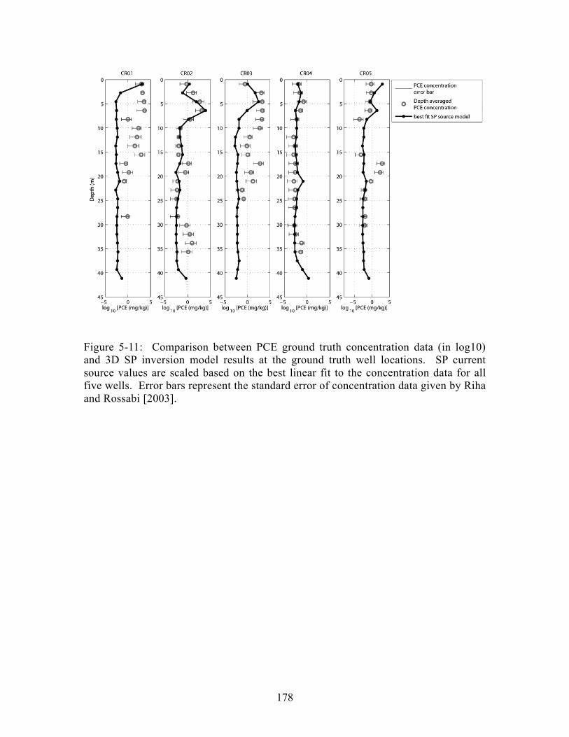
178

Figure 5-11: Comparison between PCE ground truth concentration data (in log10) and 3D SP inversion model results at the ground truth well locations. SP current source values are scaled based on the best linear fit to the concentration data for all five wells. Error bars represent the standard error of concentration data given by Riha and Rossabi [2003].

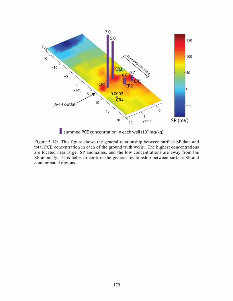
179

Figure 5-12: This figure shows the general relationship between surface SP data and total PCE concentration in each of the ground truth wells. The highest concentrations are located near larger SP anomalies, and the low concentrations are away from the SP anomaly. This helps to confirm the general relationship between surface SP and contaminated regions.

181

Chapter 6

Accounting for mis-ties on self-potential surveys with complicated acquisition geometries

6.1 Introduction

Geophysical surveys often consist of multiple transects of data collected on regular or

irregular grids with multiple crossover points. These data are collected with the goal

of uniquely defining some geophysical parameter (electrical potential, gravity, tem-

perature, bathymetry, etc.) over the survey area. Measurements are inherently imper-

fect, however, and may be contaminated by unknown random and systematic errors.

Mis-ties (also called misclosures or crossover errors) at intersection points result from

the accumulation of these imperfect measurements along different survey lines. A

successful analysis of the measured data will uniquely define the underlying field val-

ues such that they best represent the data, subject to available measurement error sta-

tistics or model constraints.

Several previous studies have addressed the geophysical mis-tie problem from

various perspectives [e.g. Cowles, 1938; Foster et al., 1970; Johnson, 1971; Prince

and Forsyth, 1984; Bandy et al., 1990]. In this paper, we present an efficient method

for processing self-potential data collected with multiple reference points and inter-

connected survey loops, though this methodology can be easily adapted to various

182

geophysical survey types. The data processing procedure proposed in this study is

robust because: (1) it produces a unique set of electric potentials for arbitrarily com-

plicated survey geometries, (2) it naturally incorporates error statistics and model

constraints, (3) it can efficiently process data in real-time as it is collected, and (4) it

reduces to traditional methods in the absence of survey complexity.

There are numerous examples of self-potential surveys with interconnected acqui-

sition lines that would benefit from this technique [e.g. Corwin and Hoover, 1979;

Michel and Zlotnicki, 1998; Finizola et al., 2003; Yasukawa et al., 2003; Aizawa,

2004]. All of these studies involve a large survey area with limited roads or paths

along which measurements are taken, in addition to sometimes rough terrain, which

necessitates the use of multiple interconnected survey lines. When two closed acqui-

sition loops share two or more common measurement locations, their crossover errors

are no longer independent and the final survey map will depend on the order in which

the lines are processed. This can become significant when there are many intersecting

survey lines with multiple crossover points.

Our proposed method produces a unique solution for the electric potential field by

processing all of the collected data simultaneously in a survey-consistent approach.

Measurements are expressed as a linear system of equations, and the entire system is

solved to minimize the misclosures over the entire survey. Traditional least squares,

which minimizes the l2 norm of the difference between measured and predicted data,

is the simplest approach to this problem. We also explore the use of an l1 measure of

misfit, which can be more robust in the presence of unreliable measurements

[Claerbout and Muir, 1973; Farquharson and Oldenburg, 1998] that can occur with

self-potential surveys, but is computationally more expensive.

6.2 Self-potential data acquisition

Values of the electric potential in a self-potential survey are given with respect to an

arbitrary reference station, which is typically assigned a value of 0 mV for conven-

ience. When possible, it is preferable to measure the potential between each survey

183

station and the fixed reference with a variable length of wire, directly measuring the

potential field and eliminating the need for extra processing. When surveys span

large areas over rough terrain, however, the length of wire that can be deployed at one

time is often limited. In this case, measurements are made with respect to a single

reference until the maximum amount of wire is deployed. This last survey location

then becomes the new reference, and measurements continue from this point. The

electric potential measured at the second reference site from the original reference

must be added to each of the potentials measured relative to the second reference sta-

tion. In this fashion, multiple lines can be tied together to cover large areas using suc-

cessive references.

A limiting case of this method is called the gradient configuration, where a fixed

length of wire equal to the minimum station spacing is used. The difference in elec-

tric potential is measured between the two stations, and then both electrodes move

forward one wire length so that the rear electrode takes the position of the front elec-

trode during the previous measurement. Again, starting from a reference value of 0

mV at the first station, the potential differences are integrated along the survey line to

compute the potential at each survey point with respect to the reference.

Two electrodes in direct contact with one another should have no potential differ-

ence between them. In practice, however, electrode drift can result in a small poten-

tial difference between electrodes (sometimes up to a few mV) when they are in direct

contact. Unaccounted for, this small difference can produce large cumulative errors

using the gradient method, as the bias is integrated over many measurements. An-

other possible systematic source of error involves telluric currents, which can result in

measurable potentials when the electrode separation is relatively large (several

mV/km). Random errors associated with electrode contact, instrumentation, and cul-

tural noise are also important to consider.

Kirchoff’s voltage law (6.1) requires that the total potential drop around any

closed survey loop must equal zero.

0V dl∆ ⋅ =∫ (6.1)

184

Due to measurement errors, however, this does not always occur and a mis-tie is

manifested at the closure point. A common means of accounting for this is to evenly

distribute the misclosure errors for each loop among the measurements in that loop

[Corwin, 1990]. This is a useful way to account for accumulated errors, but can be-

come complicated if multiple connected loops share segments.

There is a sequence implied in this traditional method of collecting and processing

data described above: each line of data is processed individually, lines are tied to-

gether at their intersections, and loop closure errors are distributed as they are in-

curred. A self-potential survey with interconnected tie-points and loops that share

segments can no longer be processed sequentially because the loops are not independ-

ent. Numerous solutions for the potential field can be found simply by processing

lines of data in different order. Our proposed method for calculating the potential

field accounts for all data points simultaneously, thereby eliminating this problem. In

addition, measurement statistics or model constraints can easily be incorporated into

the procedure.

6.3 Methodology

A simple synthetic example fashioned after that of Cowles [1938] is used to illustrate

the methodology for calculating the potential field from a set of gradient self-potential

measurements. Figure 6-1a shows an example with ten stations, where the size and

shade of the marker at each station indicates the ‘true’ potential at each point. An in-

terpolated map of the potential field is illustrated in Figure 6-1b. Synthetic, noise-

free, gradient SP data are calculated by taking the difference between adjacent poten-

tials for each of the 13 measurements along four traverses (a-d), indicated by the dif-

ferent line styles that connect points. Each traverse forms a closed loop, and no

measurements are repeated. That is, the potential between stations 4 and 5 is meas-

ured on ‘line a’, and therefore does not need to be re-measured on ‘line b’. The simu-

lated field data are summarized in Table 6-1.

185

Table 6-1: Simulated self-potential dataset for the synthetic example in Figure 6-1. Measurement

number Survey Line

Rear electrode station #

Front electrode station #

Measured SP (mV)

1 a 1 2 15 2 a 2 3 10 3 a 3 4 5 4 a 4 5 -20 5 a 5 1 -10 6 b 4 6 -5 7 b 6 7 -5 8 b 7 5 -10 9 c 2 8 -5 10 c 8 9 5 11 c 9 3 10 12 d 9 10 5 13 d 10 6 5

A critical bookkeeping step requires that each station is assigned a unique number,

even though some stations are used for more than one measurement. In practice, sta-

tions numbers are incremented by one at each new measurement location. When a

new measurement ties into a station already used on a previous line, it is important to

record the original station number.

Given M = 13 measurements and N = 10 stations in this example, the relationship

between the unknown potentials (v = [v1 … vn]T) and measured gradients (d = [∆v1 …

∆vm)]T) can be written as a system of linear equations given in equation (6.2),

= +Av d e (6.2)

where e is a vector of the unknown measurement errors. A is the connectivity (or to-

pology) matrix that describes the acquisition geometry and connects measurements to

their uniquely numbered stations. The connectivity matrix is sparse and contains only

1, -1, and 0 entries. Each measurement produces one row in A: 1 is placed in the col-

umn corresponding to the unique station number for the front electrode, -1 in the col-

umn corresponding to the rear electrode station number, and 0 in the remaining col-

umns. When each row is multiplied by v, the result is a simple expression for a po-

tential difference, vi – vj, associated with the measured value ∆v in the same row of d.

186

Because only differences are involved in each measurement, all of the rows of A

add up to zero; therefore the columns are not linearly independent, and the potentials

can only be determined up to an arbitrary constant. By assigning a value (typically

0mV) to the global reference point for the survey, the column of A associated with the

reference location is removed. This guarantees that the number of data is at least

equal to (and possibly greater than) the number of unknown parameters, depending on

whether survey lines form closed loops. As long as all of the survey stations are

connected through one or more reference locations, the problem of determining the

potential field relative to a global reference point is a well-posed problem.

We define an objective function in equation (6.3) that is a measure of data misfit

plus a regularization functional using the l2 norm.

( ) 2 2

22d m d mφ φ λΦ = + = +W d - Av W v (6.3)

Wd is a diagonal data-space weighting operator that incorporates information about

the measurement errors, where entries are typically the inverse of the estimated stan-

dard deviation for each measurement (i.e. 1d

−=W σ I ). Wm is a model-space regulari-

zation operator that provides additional model constraints. In this study, we choose 2

m l= ∇W to promote solutions for the potential field that are spatially smooth, where

l∇ is the gradient in the direction of the acquisition line. mW can therefore be com-

puted for arbitrary station spacing ix∆ using equation (6.4),

2Tm =W A X A (6.4)

where

( ) 1

0i

ijx i jX

i j

−⎧ ∆ =⎪= ⎨≠⎪⎩

. (6.5)

λ is a tradeoff parameter that provides a balance between data misfit and model

smoothness. Minimization of equation (6.3) results in the traditional linear system of

equations (6.6) that produces an estimate of the potential field, v .

( )T 2 T 2Td m m dλ+ =A W A W W v A W d . (6.6)

187

The model regularization term, mφ , is not strictly required to provide a stable in-

version result, but is used to prevent over-fitting the data in the presence of noise. We

compute φd for multiple values of λ, and interpolate to find the value of the tradeoff

parameter that results in a data misfit equal to a pre-selected target misfit value, tardφ .

Assuming Gaussian measurement errors with known standard deviation, we use a tar-

get misfit value equal to the number of measurements, M. Alternatively, one could

use the L-curve method [e.g. Hansen, 1992] to choose a value for λ that provides a

tradeoff between dφ and mφ .

For the synthetic example in Figure 6-1, we add Gaussian noise with 2.5mVσ =

(30% of the mean of the noise-free data) to the 13 synthetic measurements. Figure

6-2 shows the result of implementing equation (6.6) with 0.022λ = so that

13tard dφ φ= = . The inversion successfully recovers the original potential field such

that it is able to predict the measured data within the expected errors, as can be seen

in Figure 6-2a-b.

Cowles’ [1938] approach to closing slope (gradient) data traverses using least

squares is equivalent to the methods proposed here. Instead of the connectivity ma-

trix, however, an edge-loop matrix is used to represent the four independent loops in

the survey. The four parameters found by inverting this matrix are Lagrange multipli-

ers, and linear combinations of them produce the minimal slope correction terms that

are equal to the elements of ( −d Av ). The corrected slopes are found such that the

loop closure errors are minimized, which produces the same potential field as the

connectivity matrix method. The two methods are essentially the same; the only dif-

ference is in their application. The connectivity matrix approach presented in this pa-

per is appropriate for geophysical surveys because it can be constructed efficiently as

data is collected, while finding the independent loops in a complicated network may

not be obvious.

One drawback to the commonly used l2 norm is the strong influence of outliers on

the solution. There are numerous mechanisms that can result in large measurement

errors during a self-potential survey such as cultural noise, poor electrode contact, or

188

strong near-surface heterogeneity. An alternative, though slightly more computation-

ally expensive, approach to the mis-tie problem is to use an l1 measure of data misfit,

which is less sensitive to erratic measurements [Claerbout and Muir, 1973]. This re-

quires an iterative solution technique [Schlossmacher, 1973; Scales et al., 1988],

sometimes referred to as iteratively re-weighted least squares (IRLS), whereas the l2

method can be solved in a single step. We follow the method of Farquharson and

Oldenburg [1998] to define a set of equations that minimize the objective function

using an l1 norm. The details of this approach are presented in the appendix of this

paper, and a synthetic example is presented in the next section that compares the use

of the l1 and l2 measures of misfit.

6.4 Application to a synthetic example using the l1 norm

A larger synthetic example is used to illustrate the utility of the l1 measure of misfit

for the self-potential survey mis-tie problem, particularly when the data contain out-

liers. The Matlab “peaks” function is used as the “true” potential field for this exam-

ple, shown in Figure 6-3a, where the range of approximately 140mV is typical of

many self-potential surveys. The units of distance are arbitrary since we are only in-

terested in potential differences between survey stations.

A grid of six survey lines (a-f) is used to simulate a self-potential survey, which

are also marked on the figure. Each line consists of 49 stations, though several sta-

tions are repeated on multiple lines at the intersection points, giving a total of N = 285

unique stations. The station potentials (vtrue) sampled from the “true” potential field

in Figure 6-3a are illustrated in Figure 6-3b. A self-potential survey is simulated us-

ing the gradient method along each survey line, so that the data represent potential

differences between adjacent stations. Figure 6-3c shows the synthetic self-potential

data (d) along each line, with a total of M = 288 measurements.

First, purely Gaussian noise with 0.96mVσ = (30% of the mean of the noise-free

data) is added to the measurements. A, Wd, and Wm are constructed according to the

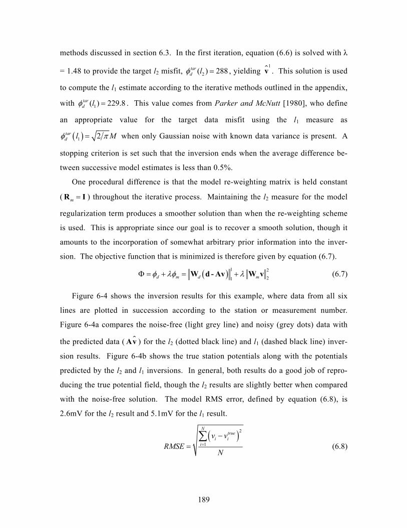
189

methods discussed in section 6.3. In the first iteration, equation (6.6) is solved with λ

= 1.48 to provide the target l2 misfit, 2( ) 288tard lφ = , yielding

1v . This solution is used

to compute the l1 estimate according to the iterative methods outlined in the appendix,

with 1( ) 229.8tard lφ = . This value comes from Parker and McNutt [1980], who define

an appropriate value for the target data misfit using the l1 measure as

( )1 2tard l Mφ π= when only Gaussian noise with known data variance is present. A

stopping criterion is set such that the inversion ends when the average difference be-

tween successive model estimates is less than 0.5%.

One procedural difference is that the model re-weighting matrix is held constant

( m =R I ) throughout the iterative process. Maintaining the l2 measure for the model

regularization term produces a smoother solution than when the re-weighting scheme

is used. This is appropriate since our goal is to recover a smooth solution, though it

amounts to the incorporation of somewhat arbitrary prior information into the inver-

sion. The objective function that is minimized is therefore given by equation (6.7).

( ) 1 2

21d m d mφ λφ λΦ = + = +W d - Av W v (6.7)

Figure 6-4 shows the inversion results for this example, where data from all six

lines are plotted in succession according to the station or measurement number.

Figure 6-4a compares the noise-free (light grey line) and noisy (grey dots) data with

the predicted data ( Av ) for the l2 (dotted black line) and l1 (dashed black line) inver-

sion results. Figure 6-4b shows the true station potentials along with the potentials

predicted by the l2 and l1 inversions. In general, both results do a good job of repro-

ducing the true potential field, though the l2 results are slightly better when compared

with the noise-free solution. The model RMS error, defined by equation (6.8), is

2.6mV for the l2 result and 5.1mV for the l1 result.

( )2

1

Ntrue

i ii

v vRMSE

N=

−=

∑ (6.8)

190

Next, we illustrate the effect of outliers in the data by increasing the level of noise

at 10% of the measurement locations, chosen randomly throughout the survey. At

these locations, 4.8mVσ = , which is five times the standard deviation of the noise for

the rest of the measurements. No prior knowledge about the outliers is assumed, so

the same values for the data weighting matrix and target misfit are maintained as in

the previous example ( 10.96m−=W I , ( )2 288tar

d lφ = , and ( )1 229.8tard lφ = ). In general,

one might need to increase the value of the target misfit when outliers are present in

order to avoid over-fitting the data. The inversion runs for 21 iterations before the

model changes are small enough to meet the stopping criterion, which is similar to the

case without outliers that runs for 25 iterations.

Figure 6-5 shows the inversion results for the case with unexpected erratic data.

In Figure 6-5a, the difference between the l2 (dotted black line) and l1 (dashed black

line) penalties on the data residual is apparent. As expected, the l2 result tends to

over-fit the data due to the quadratic penalty on the residuals. Several locations

where this is most evident are highlighted by black arrows. Figure 6-5b shows the

corresponding station potentials predicted by the two inversion methods compared

with the true solution. Large errors in the potentials of up to ~20mV can be seen in

the l2 solution, while the l1 solution avoids these artifacts. Quantitatively, the model

errors according to equation (6.8) are 7.8mV and 4.7mV for the l2 and l1 solutions,

respectively. Compared with the previous example where there were no outliers, the

l2 model error has tripled while the l1 model error has decreased slightly. This com-

parison somewhat under-represents the success of the l1 result that is observed in

Figure 6-5b, however, since equation (6.8) provides the mean model error over all sta-

tions and the greatest improvements occur at a limited number of stations.

These results confirm the general behavior that we expect: the l1 measure of misfit

produces a more robust solution in the presence of outliers. In the case where the data

contain only Gaussian noise, the l1 and l2 measures of misfit produce similar solu-

tions. There are a few locations where the l2 solution provides a slightly better result

in both examples, though the improvements are not dramatic considering the level of

191

noise. The extra computational cost for the l1 method arises from solving equation

(B.5) multiple (often ~10 to 20) times, but is by no means prohibitive.

6.5 Self-potential field example from Nevis, West In-dies

A self-potential survey was carried out on the island of Nevis (Figure 6-6) in August

2004 as a part of a larger geothermal exploration campaign supported by the Organi-

zation of American States (OAS) Geo-Caraïbes program. The data were collected us-

ing the gradient electrode configuration with a fixed separation of about 75m. An

area of approximately 16km2 was covered by 19 lines of data collected along accessi-

ble roads and trails in the southwest part of the island. The dataset consists of 483

potential difference measurements using 469 unique stations. The lines of data make

up a complicated network of measurements with many interconnected loops (Figure

6-6). The data were corrected for electrode drift by periodically placing the two elec-

trodes in direct contact, and telluric corrections were deemed unnecessary, though

may remain a small source of error in the data. Difficulties in calculating a unique

potential field by sequentially tying lines together and distributing closure errors ne-

cessitated the survey-consistent approach developed in this paper.

These drift-corrected data are inverted using the methods developed in this paper.

In this field study, however, we do not know the true standard deviation of the meas-

urement errors, or to what extent outliers are present in the data. We therefore show

several inversion results using different combinations of values for 1d σ −=W I and

tardφ to get a sense of the range of possible solutions. Each inversion assumes a con-

stant value of σ (either 2mV or 5mV) for all measurements, and two possible values

for the target data misfit. The target misfit is set to ( )2 483tard l Mφ = = and

( )2 1.5 724.5tard l Mφ = = for the l2 inversions, and ( )1 2 385.4tar

d l Mφ π= = and

( )1 1.5 2 578.1tard l Mφ π= = for the l1 inversions. Thus, four different solutions are

computed for each of the l2 and l1 methods.

192

Figure 6-7 illustrates the inversion results extracted along two of the longest sur-

vey lines, labeled ‘line a’ and ‘line b’ in Figure 6-6. In Figure 6-7a, the measured

self-potential data (black dots) are compared with the predicted data ( Av ) for the l2

(black shaded line) and l1 (grey shaded line) inversions. The width of each line repre-

sents the range of results from the four different cases of target data misfit and as-

sumed measurement standard deviations, while the white dashed line represents the

mean result. Inverted station potentials ( v ) along these two lines are shown in Figure

6-7b. The width of each shaded area again represents the range of solutions recovered

from the four different inversion runs, and the white dashed line is the mean result.

The range of possible solutions is generally larger for the l1 results due to the weaker

constraint on the data misfit for this method.

The l2 and l1 solutions mostly follow the same trends, though there is a spatially

variable offset between the two results due to the effect of outliers on the inversion.

This can be explained by considering a single line of potential difference data that is

integrated to compute the station potentials, with a single data outlier in the middle of

the line. The l2 potentials will have a large step jump at the location of the outlier,

whereas the l1 potentials, which avoid integrating the outlier, will not have the step

jump. Therefore, the two results will be similar up to the location of the outlier, but

will be offset by a constant value (equal to the magnitude of the outlier) for the re-

mainder of the line. The results in Figure 6-7 are somewhat more complicated be-

cause the entire survey is inverted simultaneously, and the shifts in Figure 6-7b can be

due to outliers in Figure 6-7a as well as outliers from other survey lines.

Figure 6-8a shows the mean l2 inverted potential field interpolated over the entire

survey area, and Figure 6-8b shows the mean l1 result using the same color scale. As

noted in Figure 6-7b, the two solutions have a similar trend, but are offset at most sur-

vey locations. Figure 6-8c shows the difference between l2 and l1 solutions, which is

almost always positive, but varies spatially with an average value of approximately

35mV over the entire survey area. There are specific regions where the two solutions

are significantly different, such as the increased (~50mV) broad negative anomaly for

the l1 result along ‘line a’ from around 1000m - 2500m relative to the start of the line

193

(0m), where the potentials for the l1 and l2 results are the same (Figure 6-7b). This

increased negative anomaly is clearly evident in Figure 6-8b-c over several survey

lines in the area between 62.61ºW - 62.62ºW and 17.12ºN - 17.13ºN.

Figure 6-9 highlights the benefit of using the survey consistent method discussed

in section 6.3 to minimize the loop closure errors globally, rather than the traditional

method of processing lines sequentially. This figure shows three different calcula-

tions of the station potentials interpolated over the whole survey area, where individ-

ual lines of data were processed in different sequences. This technique results in non-

independent loop closures and significantly different images depending on the arbi-

trary order in which the data are processed. Note, however, that the linear interpola-

tion used to generate the original results in Figure 6-9 produces less smooth images

than the interpolation used to generate Figure 6-8. While this accounts for some of

the visual differences between figures, the main effect is due to the difference in in-

version methods. We conclude that the survey-consistent approach, whether using the

l2 or l1 measure of misfit, provides a significantly more robust approach to processing

self-potential data.

6.6 Conclusions and future work

Self-potential surveys acquired with interconnected survey loops require processing

techniques that account for the fact that loop closure errors are not independent. The

methodology presented in this paper provides a simple and robust procedure for com-

puting potentials in a survey-consistent fashion. This method is valid for arbitrarily

complicated survey geometries, and is equivalent to traditional line-by-line processing

methods when survey loops are not interconnected. Our development has involved

only self-potential surveys, though this approach can easily be adapted to other geo-

physical methods.

Formulated as a linear inverse problem, this technique can easily incorporate sta-

tistical information regarding measurement errors and model constraints based on

prior information. Additionally, we have shown the utility of solving the problem us-

194

ing an l1 measure of misfit when outliers are present in the data. The l1 and l2 solu-

tions produce similar results when the noise is solely Gaussian, though the former

case requires an additional computational cost to solve the problem iteratively.

These methods can be readily adapted to provide a real-time self-potential map-

ping system. A handheld PC with a GPS antenna and data logger can record potential

differences at stations in the field. The topology matrix (A) can therefore be con-

structed as the data are collected, and updated self-potential maps can be computed at

any time. Even for relatively large surveys with several hundred stations, the compu-

tation time will be on the order of several minutes. This information can be used im-

mediately to make decisions regarding where more data should be collected.

6.7 Acknowledgements

I thank Mark Lambrides and the Organization of American States for funding the field

component of this study carried out in Nevis. Additionally, I am grateful to the other

members of the geophysical survey team: Yervant Vichabian, Darrell Coles, Mary

Krasovec, Colin Morgan, Timur Kanachet, and Dale Morgan. GPS survey positions

were provided by Dr. Richard Robertson and Rosemarie Mohais of the Seismic Re-

search Unit, University of West Indies, Trinidad.

195

Figure 6-1: Synthetic example of a gradient SP survey with 10 stations and 13 meas-urements (based on Cowles [1938]). a) Symbol size and shading represents the ‘true’ station potentials. Gradient data are simulated along four lines (a-d) by calculating potential differences between adjacent stations. b) Interpolated potential field using the 10 stations in a).

196

Figure 6-2: Illustration of the l2 inversion results for the data from Figure 6-1 with additional Gaussian noise. The inversion method is able to successfully predict meas-urements within the expected errors. a) True data that would be measured from the potentials in Figure 6-1a (grey line) with error bars to denote the standard deviation of the added noise, and one realization of noisy measurements (black dots). b) Interpo-lated potential field found by inverting the noisy measurements.

197

Figure 6-3. Synthetic potential field used to illustrate mis-tie methods. a) Map of the complete potential field with six survey lines annotated. b) True potentials at the sur-vey stations (49 per line, 294 total). c) Synthetic gradient data (potential differences between adjacent stations) for each of the survey lines.

198

Figure 6-4. Inversion results for the case with Gaussian noise only (σ = 0.96mV). All six lines are displayed sequentially as a function of survey measurement # or station #. a) Comparison of the synthetic noise-free (light grey line) and noisy (grey dots) data with data predicted by the l2 inversion (black dotted line), and the l1 inversion (black dashed line). b) Comparison of the true station potentials (light grey line) with the results from the l2 inversion (black dotted line), and the l1 inversion (black dashed line).

199

Figure 6-5. Inversion results for the case where 10% of the measurement locations have an unexpectedly large measurement error (σ = 4.8mV) to simulate outliers. All six lines are displayed sequentially as a function of survey measurement # or station #. a) Comparison of the synthetic noise-free (light grey line) and noisy (grey dots) data with data predicted by the l2 inversion (black dotted line), and the l1 inversion (black dashed line). b) Comparison of the true station potentials (light grey line) with the results from the l2 inversion (black dotted line), and the l1 inversion (black dashed line). Black arrows highlight several of the locations most affected by the outliers.

200

Figure 6-6. Map of Nevis showing the station locations for 19 lines of gradient SP data over an area of approximately 16km2 in the southwest part of the island. The two lines with different shading (labeled a & b) are used for displaying results in subse-quent figures.

201

Figure 6-7. Inversion results for the field dataset shown along ‘line a’ and ‘line b’ from Figure 6-6. The width of each filled area represents the range of results that are found using different combinations of σ and tar

dφ for the l2 and l1 measures of misfit, while the white dashed line represents the mean result. a) Comparison of the field SP measurements (black dots) with predicted data ( Av ) from the l2 (black area) and l1 (grey area) inversions. b) Range of station potentials predicted along the two tran-sects for the different combinations of σ and tar

dφ for the l2 and l1 measures of misfit.

202

Figure 6-8. Potential field maps calculated using the l2 (a) and l1 (b) inversion meth-ods, interpolated over the entire survey area. In both cases, the mean result from us-ing four different combinations of data weights and target misfit values is illustrated, which corresponds to the white dashed lines in Figure 6-7. c) The difference between the mean l2 and l1 solutions varies in magnitude over the entire survey area, but is almost always positive.

203

Figure 6-9. Three different versions of the potential field computed using traditional processing methods with lines of data processed in different orders, then interpolated over the entire survey area. Loop closure errors are distributed along new loops as they are completed, but potentials along existing loops are not modified. Because the loops are not independent, this methodology produces inconsistent results.

205

Chapter 7

Conclusions and future research directions

7.1 Conclusions

The self-potential method has met with mixed success over many years of use, but has

yet to become a truly “mainstream” geophysical technique. This is not for a lack of

trying, however; self-potential surveys have been carried out for a wide variety of ap-

plications. Measurements are fairly straightforward and inexpensive to carry out, and

the data can sometimes be interpreted qualitatively with reasonable success. I see

three main research areas needed to promote the wider implementation of self-

potential investigations, several of which I have attempted to address in this disserta-

tion:

1. Better understanding the physics and chemistry of self-potential source

mechanisms, particularly in the context of how these sources are distributed in

the earth under realistic conditions.

2. Improved data processing and interpretation algorithms that provide a quanti-

tative framework for characterizing self-potential sources.

3. Improving data acquisition methods and equipment to improve the quality of

measured signals and better quantify measurement errors.

This thesis has focused primarily on the second point by introducing a general ap-

proach for the three-dimensional source inversion of self-potential data. Incorporat-

206

ing resistivity information into the inverse method is an important step, as unknown

resistivity structure can be a significant source of error in the self-potential data

analysis. Not only is resistivity information useful for the self-potential data analysis,

but these methods provide complementary information about the subsurface. There-

fore, it is generally advantageous to conduct joint resistivity and self-potential surveys

where possible.

There is a natural feedback between the second and first points above. Informa-

tion gained from better understanding self-potential source mechanisms will aid our

ability to image these targets in the earth by incorporating realistic prior information

into the inverse problem. For example, the constraint that sources should be spatially

compact as utilized in this thesis works well for many source inversion problems. A

more powerful approach will be to also incorporate constraints based on the physics

and chemistry of the coupling mechanisms.

In the other direction, source inversion of self-potential observations can provide

useful insights into the behavior of source mechanisms, particularly for realistic cases

in the earth that cannot be readily studied through numerical simulations or laboratory

experiments. Returning to the analogy of understanding earthquakes, it is through

both the interpretation of recorded seismograms as well as theoretical or laboratory

studies of stress and deformation in earth materials that the problem is fully ad-

dressed. Similarly with self-potentials, an understanding of the source mechanisms in

the earth will come from reconciling observations with the known behavior of the

coupling phenomena.

Finally, careful consideration should be given to improving data quality for self-

potential surveys. Many advances in geophysical methods have come from improv-

ing both the quality and quantity of measured data allowed by modern recording

equipment. Reducing and quantifying measurement errors are important acquisition-

related aspects that have a significant impact on inversion results. At a minimum,

data should be collected to avoid spatial aliasing of the signal. Significant improve-

ments in sensitivity can be made for smaller field-scale experiments, where additional

measurements can be made at depth in boreholes

207

7.2 Future research ideas: secondary source imaging

One of the main drawbacks of the self-potential method is that there is significant un-

certainty associated with the fact that it is a passive technique. Given the three gen-

eral components of a survey (source, medium properties, and response), only the re-

sponse is known. In this section, I highlight a new self-potential imaging technique

that utilizes water pumped to/from a well as a known source, which can be used to

image unknown sources in the subsurface away from the well. This has a significant

advantage from traditional self-potential methods as it incorporates information from

a known source and, as discussed below, also naturally accounts for unknown resistiv-

ity heterogeneity near the well.

This technique is based on the discussion surrounding equation (2.50), where the

first term ( 2L P∇ ) is associated with the source/sink of fluid at the well, and is called

the “primary” source. In section 2.3, the primary source was found to be constant for

a given pumping rate, and located in close proximity to the screened portion of the

well (Figure 2-14). The second term in equation (2.50), ( L P∇ ⋅∇ ) is the “secondary”

source, and is associated with fluid flow across boundaries of the coupling coefficient

in the subsurface away from the well.

Consider the situation illustrated in Figure 7-1. A well (blue column) is located on

the left side of the figure, where the screened section is shaded light blue. An un-

known structure (fault, intrusion, etc.) with different resistivity and coupling coeffi-

cient from the background medium is shown in brown towards the right side of the

figure. Self-potential electrodes are placed in an array on the earth surface, shown by

black triangles.

When fluid is pumped from the well (Figure 7-1a), the recorded self-potential re-

sponse will be a superposition of the primary source at the well plus the secondary

source induced by fluid flow across the boundary. In the second step (Figure 7-1b),

the well pump is turned off, and an electric pole source is lowered into the screened

portion of the well. In practice, this would likely involve a second current electrode

208

placed far away from the well and measuring electrodes. The potential field due to

the active current source in the well is then recorded.

Differencing these two datasets leaves only the potential field that is due to the

unknown secondary source, which can be subsequently imaged using the inversion

techniques developed in this thesis. Because we know that there will be a large

source at the well for a pumping experiment, it is advantageous to remove this effect

in order to highlight the more subtle secondary sources. This is accomplished by rec-

ognizing that the potential field due to the source at the well can be simulated by an

active source at the well screen, though a long screened section of the well may begin

to appear as a line source rather than a point.

There is an additional subtle, yet extremely important, benefit to this technique.

The potential field recorded from the active source in the well (Figure 7-1b), incorpo-

rates all of the unknown resistivity structure of the medium. That is, the response

provides the empirical Green’s functions for the medium from the well to the meas-

urement locations. When this response is subtracted from the response in Figure 7-1a,

the effect of the source and the unknown resistivity structure are removed. The shape

of the anomaly in Figure 7-1a is defined both by the secondary sources and any resis-

tivity heterogeneity. Without prior information, it is not possible to distinguish be-

tween these influences. In Figure 7-1b, however, the anomaly is related solely to the

resistivity structure. Thus, combining these two datasets removes the influence of the

resistivity structure, without having to know the resistivity explicitly.

Inversion of the residual self-potential signal (Figure 7-1a minus Figure 7-1b) still

requires some resistivity assumption, however, because the true Green’s functions

from the secondary source to the receivers remain unknown. While these assumptions

will lead to some uncertainty, as discussed in Chapter 4, the overall benefit of remov-

ing the effects of the primary source at the well is significant.

209

Figure 7-1: Conceptual schematic of a self-potential secondary source imaging ex-periment. When fluid is pumped from the well (A), the self-potential response is re-corded due to both source types: fluid withdrawal at the well and flow across a boundary. Next, an electric pole source is placed in the screened portion of the well while it is no longer pumping, and the potential field is recorded at the surface (B). Differencing the two datasets leaves only the potential field that is due to induced flow across a boundary.

211

Appendix A

Discretization using the transmis-sion network equations

The transmission network analogy is a useful method for the discretization of the dif-

ferential equations that govern geophysical forward and inverse problems [Madden

and Swift, 1969; Swift, 1971; Madden, 1972]. The resulting linear system of equa-

tions is essentially the same as would be obtained using finite difference or finite

element methods. Analogy to transmission network systems provides useful insight

for the self-potential problem, where the governing equations come from the electro-

static form of Maxwell’s equations.

( ) ( ) ( ), , , , , ,x y z x y z x y z∇ = − ⋅φ ρ j (A.1)

( ) ( ), , , ,x y z x y z∇ ⋅ =j f (A.2)

Thus, the electric field, = −∇E φ [V·m-1], is determined by the earth resistivity struc-

ture, ρ [Ω·m], and current density, j [A·m-2]. Equation (A.2) is the continuity condi-

tion on the current density, which is divergence-free in the absence of external electric

sources, f [A·m-3]. Combining equations (A.1) and (A.2) yields a Poisson equation,

( , , ) ( , , ) ( , , )x y z x y z x y z−∇⋅ ∇ =σ φ f , (A.3)

where 1−=σ ρ represents the conductivity.

212

Equation (A.1) can be approximated using the network analogy, in which a con-

tinuum is discretized into network nodes and impedance branches (Figure A-1). Fol-

lowing the convention of Zhang et al. [1995] and Shi [1998], the earth is divided into

resistivity blocks ρ(i,j,k) with a node at the top center of each block. In three dimen-

sions, each interior node is connected to six surrounding nodes by an impedance

branch (Figure A-1). The impedance of a branch is defined by the simple relationship

between resistivity, length, and cross-sectional area.

LRA

ρ= (A.4)

In the self-potential problem, we are not concerned with complex impedances; each

branch is therefore associated simply with a resistance (with units of ohms).

Due to the convention of placing a node at the top center of a resistivity block, in-

terior branches in the x-y plane span four blocks; two above and two below (Figure

A-2). These branch impedances are therefore given by the parallel combination of

two pairs of impedances that are each connected in series. In the z-direction, an im-

pedance branch is determined completely by a single resistivity block. The branch

impedances are therefore defined by equations (A.5) through (A.7) [from Zhang et

al., 1995].

1 1( ) ( , , ) ( 1) ( 1, , )( ) ( ) ( ) ( )

1( ) ( , , 1) ( 1) ( 1, , 1)( ) ( 1) ( ) ( 1)

xx i i j k x i i j kRy j z k y j z k

x i i j k x i i j ky j z k y j z k

ρ ρ

ρ ρ

=∆ ∆ − −

+∆ ∆ ∆ ∆

+∆ − ∆ − − −

+∆ ∆ − ∆ ∆ −

(A.5)

1 1( ) ( , , ) ( 1) ( , 1, )

( ) ( ) ( ) ( )1

( ) ( , , 1) ( 1) ( , 1, 1)( ) ( 1) ( ) ( 1)

yy j i j k y j i j kR

x i z k x i z k

y j i j k y i i j kx i z k x i z k

ρ ρ

ρ ρ

=∆ ∆ − −+

∆ ∆ ∆ ∆

+∆ − ∆ − − −

+∆ ∆ − ∆ ∆ −

(A.6)

1 ( ) ( )( ) ( , , )z

x i y jR z k i j kρ

∆ ∆=

∆ (A.7)

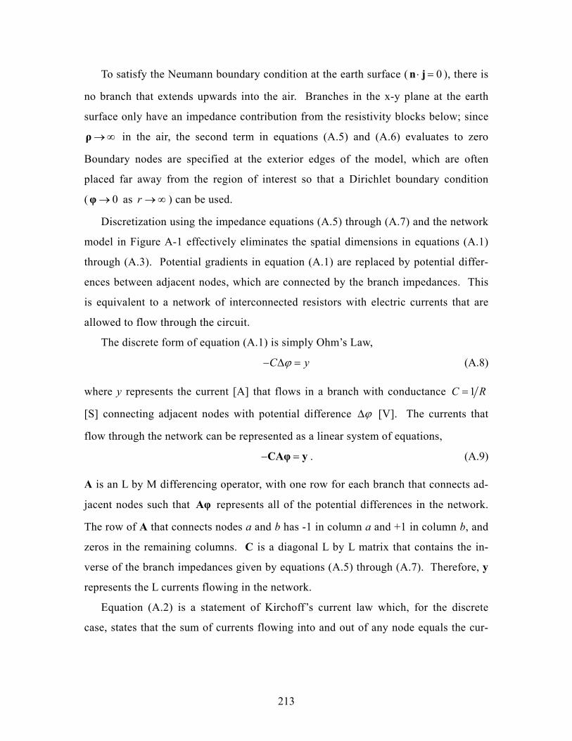
213

To satisfy the Neumann boundary condition at the earth surface ( 0⋅ =n j ), there is

no branch that extends upwards into the air. Branches in the x-y plane at the earth

surface only have an impedance contribution from the resistivity blocks below; since

→ ∞ρ in the air, the second term in equations (A.5) and (A.6) evaluates to zero

Boundary nodes are specified at the exterior edges of the model, which are often

placed far away from the region of interest so that a Dirichlet boundary condition

( 0→φ as r → ∞ ) can be used.

Discretization using the impedance equations (A.5) through (A.7) and the network

model in Figure A-1 effectively eliminates the spatial dimensions in equations (A.1)

through (A.3). Potential gradients in equation (A.1) are replaced by potential differ-

ences between adjacent nodes, which are connected by the branch impedances. This

is equivalent to a network of interconnected resistors with electric currents that are

allowed to flow through the circuit.

The discrete form of equation (A.1) is simply Ohm’s Law,

C yϕ− ∆ = (A.8)

where y represents the current [A] that flows in a branch with conductance 1C R=

[S] connecting adjacent nodes with potential difference ϕ∆ [V]. The currents that

flow through the network can be represented as a linear system of equations,

− =CAφ y . (A.9)

A is an L by M differencing operator, with one row for each branch that connects ad-

jacent nodes such that Aφ represents all of the potential differences in the network.

The row of A that connects nodes a and b has -1 in column a and +1 in column b, and

zeros in the remaining columns. C is a diagonal L by L matrix that contains the in-

verse of the branch impedances given by equations (A.5) through (A.7). Therefore, y

represents the L currents flowing in the network.

Equation (A.2) is a statement of Kirchoff’s current law which, for the discrete

case, states that the sum of currents flowing into and out of any node equals the cur-

214

rent source at the node. The discrete form of the divergence operator is T−A [Strang,

1986], so equation (A.2) becomes

T− =A y s , (A.10)

where the current source, s, has units of Amperes. Combining equations (A.9) and

(A.10) leads to the discrete version of (A.3), which represents the network as a linear

system of equations.

T = =A CAφ Kφ s (A.11)

The stiffness matrix, K, is positive definite symmetric and has a banded structure,

where the number and spacing of bands depends on the model geometry. K can be

formed from product TA CA , though it can also be formed directly according to the

rules given in equation (A.12).

1

1

1 connected to

0 not connected to

P

p np

nmnm

n mR

K n mR

n m

=

⎧ ⎛ ⎞ =⎪ ⎜ ⎟⎝ ⎠⎪

⎪⎪ ⎛ ⎞= −⎨ ⎜ ⎟⎝ ⎠⎪

⎪⎪⎪⎩

∑

(A.12)

The diagonal element on the nth row of K contains the sum of the P branch conduc-

tances that are connected to node n, where 6P = for an interior node in three-

dimensions. The mth column on the nth row contains the negative of the branch con-

ductance that connects nodes n and m, and equals zero if nodes n and m are not con-

nected. Implementation of the Dirichlet boundary condition on the boundary nodes is

accomplished by removing either the columns of A, or the rows and columns of K,

associated with the boundary nodes.

215

Figure A-1.: Schematic of a portion of the 3D transmission network discretization. Adapted from Zhang et al. [1995].

216

Figure A-2: Close-up view of a single impedance branch in the x-z plane. Rx(i,j,k) is determined by the impedance contributions from four resistivity blocks that share the branch, while each Rz comes from a single resistivity block.

218

Appendix B

Minimization using an l1 measure of data misfit

Equation (B.1) describes the general form of the objective function to be minimized.

( ) p

jj

xφ = ∑x (B.1)

Traditional least squares problems that satisfy the l2 norm are solved using 2p = . In

this case, the l1 measure of misfit is utilized with 1p = , and the objective function is

the sum of absolute values of a vector, x. This provides a framework for minimizing

a general objective term using the l1 measure, where x can represent either the data

misfit term (B.2)

( )d=x W d - Av , (B.2)

or a measure of model length given by a regularization functional (B.3).

m=x W v (B.3)

A modified form of the objective function, given by equation (B.4), is needed to avoid

the discontinuity in φ∂ ∂x for any 0ix = [Ekblom, 1987; Farquharson and Olden-

burg, 1998]. A small user-specified value, ε, introduces stability for the case where

any 0ix = .

( ) ( )11/ 22 2

1φ ε= +x x (B.4)

219

The chain rule is used to compute the derivative of the objective function with re-

spect to the unknown potentials, v. A new system of equations (B.5) that provides an

estimate of the unknown potentials is found by setting this expression equal to zero.

( )T Td d d m m m d d dλ+ =A W R W A W R W v A W R W d (B.5)

where,

( ) 1/ 22 2

0i

ijx i jR

i j

ε−⎧ + =⎪= ⎨

≠⎪⎩. (B.6)

Because R is a function of the unknown potentials, this is a non-linear system, and an

iterative approach must be used. This is sometimes referred to as iteratively re-

weighted least squares (IRLS) [Scales et al., 1988].

We again follow the approach of Farquharson and Oldenburg [1998] by setting R

= I for the first iteration, which results in the traditional least squares solution given

by equation (6.6). This estimate, k

v (k = 1), is then used to compute a new Rk+1

from equation (B.6), which is subsequently substituted into equation (B.5) to produce

a new estimate, 1k +

v . This procedure is repeated until 1k k

δ+

− <v v , where δ is a

user-specified value that determines when to stop the inversion based on the change in

model parameters between successive IRLS iterations. Assuming only Gaussian er-

rors and known data variance, an appropriate value for the target data misfit using the

l1 measure is ( )1 2tard l Mφ π= [Parker and McNutt, 1980]. In the case where out-

liers are present, however, a larger target misfit may be needed to avoid over-fitting

the data.

There are now three user-defined parameters, which are not necessarily independ-

ent from one another, that control the behavior of the solution: λ, one ε for Rd, and

one ε for Rm. Small values of ε are needed to approximate equation (B.1), but too

small a value can introduce instability for any 0ix → . Large values of ε tend to act

more like the traditional regularization parameter, λ (i.e., 1ε −→R I when ixε ).

220

Typically, a plot of ( )φ x for a range of ε is used to determine an optimal balance be-

tween these extremes [Farquharson and Oldenburg, 1998; Zhdanov and Tolstaya,

2004]. This is not computationally expensive because it only requires substituting

multiple values of ε into equation (B.4) using the current value of x. λ can be chosen

in the same fashion that is discussed in section 6.3, by searching over multiple possi-

ble values to find the one that provides the desired data misfit, tardφ .

An algorithm for solving the self-potential survey mis-tie problem using the l1

norm is summarized below:

1. Compute A, Wd, and Wm as suggested in section 6.3.

2. Set d m= =R R I .

3. Solve equation (B.5) for multiple values of λ, and find the value that produces

tard dφ φ= for the l2 measure of misfit. The corresponding

1v is the l2 solution.

4. Choose optimal values of ε for Rd and Rm by plotting dφ and mφ using equation

(B.4) with the current k

v and a range of ε.

5. Compute Rd and Rm using equation (B.6) with the current k

v and ε.

6. Update ( )1max 0.95 ,tar tar tard d d lφ φ φ⎡ ⎤= ⎣ ⎦ to provide a smooth transition between the l2

and l1 target misfit values.

7. Solve equation (B.5) for multiple values of λ, and find the value that produces

tard dφ φ= . Store the solution

kv that corresponds to the target misfit.

8. Repeat from step #4 until 1k k

δ+

− <v v .

222

Appendix C

Construction notes for Ag-AgCl porous pot electrodes

C.1 Ag-AgCl conductor preparation

Silver wire mesh is cut into rectangular strips and rolled into a cylinder. The dimen-

sions for the strips depend on the application, but we have previously used 4cm x

17cm. The strips are rolled into a cylinder using a pencil or something similar to give

them shape, then washed with acetone and de-ionized (DI) water.

Electroplating is done in a solution of approximately 1M NaCl, which needs to be

replenished after several electrodes are made. A schematic of the setup is shown in

Figure C-1. DC current is passed between the silver mesh and a non-corrosive con-

ductor in a solution of NaCl. The positive lead is connected to the mesh so that Cl-

ions are attracted to the silver. A few centimeters of mesh is left out of the solution so

that a solder joint can be made to the silver. The negative lead is connected to the

metal conductor through a multi-meter that is used to monitor the current supply. A

variable DC source is used so that the current can be controlled.

A rough estimate of the current needed is found by applying 1 Coulomb per square

cm of silver mesh. The 4cm x 17cm tube has roughly 36 cm2 of silver surface area,

which requires 6 minutes of electroplating using 100mA of current. The mesh should

be agitated occasionally to ensure an even coating of AgCl, which appears black/dark

purple (Figure C-2). Current is applied until there is an even coating of silver chlo-

223

ride, which sometimes takes a little longer than the time estimated. The mesh is

rinsed in DI water and set aside to dry.

C.2 Electrode housing preparation

The top of the electrode consists of a PVC cap with female threading and a small hole

drilled in the top for the wire lead. The cap is threaded onto a male adapter, which

has one threaded end and one slip end, and fixed with PVC cement (Figure C-3). The

slip end is a 1” fitting.

A length of wire needed for the electrode lead is cut, with a minimum of about 12

inches. The un-plated end of the silver mesh (top end in Figure C-2) is soldered to the

wire lead, being careful to solder only onto the pure silver, and not onto the AgCl. It

helps to braid some of the copper wire strands into the silver mesh before soldering.

Also, if a very long wire lead is used, it is best to feed it through the PVC cap before

soldering instead of pulling the whole length of wire though afterwards.

Next, the PVC cap is placed in a rack or vice so that the slip end is pointing up. A

board with nails spaced so that the threaded part of the cap rests on two nails works

well. Pulling down on the wire brings the mesh to the bottom of the cap, and helps

keep it nearly vertical.

Epoxy is poured into the cap until it is filled above the Ag-AgCl joint, but below

the lip on the inside of the male-slip adapter, and left to dry. No epoxy should be al-

lowed to dry in the slip end of the adapter so that the PVC tube can be inserted later,

and the mesh should stay vertical as the epoxy dries. A squeeze tube or “pastry bag”

is useful so that the epoxy can be poured to the end of the cap without getting it on

the mesh.

We tested several non-conductive/non-reactive glues and epoxies, but only had

good success with Loctite® Hysol® two part epoxy.

C.3 Electrode tube and end cap

224

The electrode tube is made of one-inch PVC pipe with a porous cup attached to the

bottom end. For gelled electrodes, the length of the tube and electrolyte properties

determine the lifetime of the electrode. The life of the electrode is given by Petiau

[2000] as

2D Tt G L k= (C.1)

where,

( ) ( )0.581.720.082 25 24 /T M M S S mG C C C C C= − − − . (C.2)

tD is the life of the electrode in days, L is the length of the electrode from the porous

cup to the bottom end of the silver mesh in mm, and k is the diffusion coefficient in

mm/day that will vary with different electrolytes. CM is the maximum electrolyte

concentration (>1 with non-dissolved salt), CS is the concentration at saturation (CS =

1), and Cm is the minimum concentration outside the electrode.

Equation (C.2) is a useful approximation and is valid for CM > CS, which means

there is non-dissolved salt added to extend the electrode lifetime. For CM = CS, Equa-

tion (C.1) is simplified to

2 / 4Dt L k= (C.3)

Based on these equations, the length of PVC tubing needed for the electrode body can

be approximated.

After the PVC tubing is cut to length, a CoorsTek porous ceramic cup (Figure

C-4) is glued inside one end with the Loctite® epoxy. The cup is inserted in the bot-

tom of the PVC tube so that the bottom of the cup extends a few millimeters beyond

the end of the PVC. The epoxy is left to dry with the PVC tube standing vertically

and the porous cup at the top. Tape or dowel rods are useful to hold the cup in place

while the epoxy dries.

After the epoxy is dry enough that the ceramic cup doesn’t slide in the PVC tube,

more epoxy should be applied around the edge of the protruding cup so that it is com-

pletely sealed (Figure C-5). Once again, the PVC/ceramic cup is left to dry in a verti-

225

cal position. When the epoxy has dried, the PVC tube is filled with water to check for

leaks.

C.4 Preparing the electrolyte and sealing the elec-trode

For a refillable liquid electrode, everything is ready; the PVC tube can be filled with a

saturated solution of NaCl or KCl, and the end cap with silver mesh is placed onto the

tube. Figure C-6 illustrates the completed electrode design. Semi-permanent elec-

trodes, however, require a solid or gelled electrolyte since they cannot be refilled.

Various electrode/electrolyte designs are discussed by Perrier et al. [1997] and Petiau

[2000].

We use a NaCl electrolyte (though KCl can also be used), which is gelled with the

addition of BactoTM Agar solidifying agent. Before starting, the following items

should be on hand: the end cap with silver mesh glued in place, the PVC tube with

ceramic cup glued in place, a vice to hold the PVC tube vertically, a funnel, and PVC

cement. To make the gel, a large beaker of DI water saturated with NaCl (365 g/L) is

heated on a hot plate. While this is heating, a few smaller beakers that are large

enough to hold enough fluid for one electrode are prepared. NaCl is added to each

beaker so that the final NaCl saturation after adding the heated saturated solution will

be CM in equation (C.2). i.e.,.if CM = 2 and the electrode volume is 100mL, 36.5g of

salt is placed in the small beaker. This will give the required twice-saturated solution

when 100mL of the heated NaCl solution is added.

When the large beaker of NaCl is hotter than 70°C, 30g/L of the Agar powder is

added and stirred constantly until the powder dissolves. When the Agar is completely

dissolved, one electrode’s-worth is poured into each beaker and is stirred continu-

ously. The temperature must be monitored continuously because it needs to be poured

into the PVC tube before it begins to rapidly gel ~40°C. If it is poured into the PVC

tube while it is still much hotter than 40°C, the gelled electrolyte will not be uniform

because the salt tends to settle to the bottom.

226

When one of the small beakers with Agar/NaCl electrolyte cools to ~45-50°C, it

begins to thicken rapidly. The gelled electrolyte should be stirred vigorously before

pouring the solution into the PVC tube, leaving about 1-2cm unfilled. PVC cement

should be immediately applied to the outside of the PVC tube and inside of the PVC

end cap. The electrode is then sealed by placing the end cap over the tube, with the

mesh in the electrolyte. These final steps of pouring the electrolyte and sealing the

electrode must be done in rapid succession so that the electrolyte does not solidify

before the mesh is placed into it.

A batch of completed electrodes is shown in Figure C-7. A balloon is placed over

the ceramic cup on the end of each electrode to keep it from drying out before use.

Cheese cloth soaked in a solution of saturated NaCl is placed inside each balloon.

We have also investigated the use of Cab-O-Sil®, a fumed silica that is used for

rheologic control in various industrial applications, as the electrolyte gelling agent.

One benefit is that the Cab-O-Sil® will form a gel when vigorously mixed in a

blender, and does not need to be heated, somewhat simplifying the electrode manufac-

ture process. A second benefit is that Cab-O-Sil® is frequently used as a solidifying

agent for back-filling boreholes used in geophysical applications; this was the case for

the electrode boreholes at the Savannah River Site discussed in Chapter 5. Minimiz-

ing the differences between the electrode material and soil in which it is placed may

help to improve the electrode performance.

227

Figure C-1: Setup for electroplating the silver mesh.

1M NaCl

silver mesh with ~2cm not in NaCl

Non-corrosive conductor

100mA

Variable DC power supply

Multi-meter set to DC current

228

Figure C-2: Silver mesh electroplated with AgCl.

229

Figure C-3: Electrode top cap configuration.

230

Figure C-4: Porous ceramic cup (from CoorsTek, Inc.).

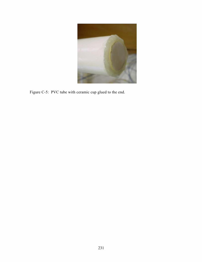
231

Figure C-5: PVC tube with ceramic cup glued to the end.

232

Figure C-6: Schematic of the porous pot electrode design.

233

Figure C-7: Completed electrodes

235

References

Acar, R., and C.R. Vogel (1994), Analysis of Bounded Variation Penalty Methods for

Ill-Posed Problems, Inverse Probl., 10 (6), 1217-1229.

Ackerer, P., A. Younes, and R. Mose (1999), Modeling variable density flow and sol-

ute transport in porous medium: 1. Numerical model and verification, Transport

Porous Med., 35 (3), 345-373.

Aizawa, K. (2004), A large self-potential anomaly and its changes on the quiet Mt.

Fuji, Japan, Geophys. Res. Lett., 31 (5), L05612, doi:10.1029/2004GL019462.

Ajo-Franklin, J.B., J.T. Geller, and J.M. Harris (2005), A survey of the geophysical

properties of chlorinated DNAPLs, Journal of Applied Geophysics.

Ajo-Franklin, J.B., B.J. Minsley, and T.M. Daley (2007), Applying compactness con-

straints to differential traveltime tomography, Geophysics, in press.

Atekwana, E.A., E. Atekwana, F.D. Legall, and R.V. Krishnamurthy (2004), Field

evidence for geophysical detection of subsurface zones of enhanced microbial

activity, Geophys. Res. Lett., 31 (23).

Atekwana, E.A., W.A. Sauck, and D.D. Werkema (2000), Investigations of geoelectri-

cal signatures at a hydrocarbon contaminated site, J. Appl. Geophys., 44 (2-3),

167-180.

Bader, S. (2005), Osmosis in groundwater: chemical and electrical extensions to

Darcy's Law, Ph.D. thesis, Technische Universiteit Delft, Delft, The Netherlands.

236

Bandy, W.L., A.F. Gangi, and F.D. Morgan (1990), Direct method for determining

constant corrections to geophysical survey lines for reducing mis-ties, Geophys-

ics, 55 (7), 885-896.

Bard, A.J., and L.R. Faulkner (1980), Electrochemical methods: fundamentals and

applications, 718 pp., Wiley, New York.

Batzle, M., and Z.J. Wang (1992), Seismic Properties of Pore Fluids, Geophysics, 57

(11), 1396-1408.

Bertete-Aguirre, H., E. Cherkaev, and M. Oristaglio (2002), Non-smooth gravity

problem with total variation penalization functional, Geophys. J. Int., 149 (2),

499-507.

Bigalke, J., and E.W. Grabner (1997), The Geobattery model: a contribution to large

scale electrochemistry, Electrochim. Acta, 42 (23-24), 3443-3452.

Birch, F.S. (1998), Imaging the water table by filtering self-potential profiles, Ground

Water, 36 (5), 779-782.

Blakely, R.J. (1995), Potential theory in gravity and magnetic applications, xix, 441

p. pp., Cambridge University Press, Cambridge [England] ; New York.

Bockris, J.O.M., and A.K.N. Reddy (1970), Modern electrochemistry; an introduction

to an interdisciplinary area, vol. 2, 1432 pp., Plenum Press, New York.

Bockris, J.O.M., and A.K.N. Reddy (1998), Modern Electrochemistry, 2nd edition,

vol. 1, 2053 pp., Plenum Press, New York.

Bockris, J.O.M., and A.K.N. Reddy (2000), Modern Electrochemistry, 2nd edition,

vol. 2B, Kluwer Academic/Plenum Publishers, New York.

Bogoslovsky, V.A., and A.A. Ogilvy (1973), Deformations of natural electric fields

near drainage structures, Geophys. Prospect., 21, 716-723.

237

Boulanger, O., and M. Chouteau (2001), Constraints in 3D gravity inversion, Geo-

phys. Prospect., 49 (2), 265-280.

Briggs, V.A., J. Sogade, B. Minsley, M. Lambert, D. Coles, P. Reppert, F.D. Morgan,

J. Rossabi, and B. Riha (2003), 3D Inversion of Induced Polarization Data from

Borehole Measurements to Map Subsurface Contaminations of Tetrachloroethyl-

ene and Trichloroethylene, Eos Trans. AGU, 84 (46), Fall Meet. Suppl. Abstract

H31B-0461.

Bube, K.P., and R.T. Langan (1997), Hybrid l1/l2 minimization with applications to

tomography, Geophysics, 62 (4), 1183-1195.

Chambers, J.E., M.H. Loke, R.D. Ogilvy, and P.I. Meldrum (2004), Noninvasive

monitoring of DNAPL migration through a saturated porous medium using elec-

trical impedance tomography, J. Contam. Hydrol., 68 (1-2), 1-22.

Chen, C., J.A. Puhakka, and J.F. Ferguson (1996), Transformations of 1,1,2,2-

tetrachloroethane under methanogenic conditions, Environ. Sci. Tech., 30 (2),

542-547.

Christensen, T.H., P.L. Bjerg, S.A. Banwart, R. Jakobsen, G. Heron, and H.J.

Albrechtsen (2000), Characterization of redox conditions in groundwater con-

taminant plumes, J. Contam. Hydrol., 45 (3-4), 165-241.

Claerbout, J.F., and F. Muir (1973), Robust Modeling with Erratic Data, Geophysics,

38 (5), 826-844.

Clerc, G., G. Petiau, and F. Perrier (1998), The Garchy 1995-1996 electrode experi-

ment technical report, INSU-CNRS/CEA, Paris.

Constable, S.C., R.L. Parker, and C.G. Constable (1987), Occam's inversion: A practi-

cal algorithm for generating smooth models from electromagnetic sounding data,

Geophysics, 52 (3), 289-300.

238

Corwin, R.F. (1973), Offshore application of self-potential prospecting, Ph.D. thesis,

University of California, Berkeley, Berkeley, California.

Corwin, R.F. (1990), The self-potential method for environmental and engineering

applications, in Geotechnical and Environmental Geophysics, Society of Explo-

ration Geophysicists, edited by S.H. Ward, Tulsa, pp. 127-146.

Corwin, R.F., and D.B. Hoover (1979), The self-potential method in geothermal ex-

ploration, Geophysics, 44 (2), 226-245.

Cowles, L.G. (1938), The adjustment of misclosures, Geophysics, 3 (4), 332-339.

Daily, W., and A. Ramirez (1995), Electrical-Resistance Tomography During in-Situ

Trichloroethylene Remediation at the Savanna River Site, J. Appl. Geophys., 33

(4), 239-249.

Darnet, M., A. Maineult, and G. Marquis (2004), On the origins of self-potential (SP)

anomalies induced by water injections into geothermal reservoirs, Geophys. Res.

Lett., 31 (19), L19609, doi:10.1029/2004GL020922.

Darnet, M., and G. Marquis (2004), Modelling streaming potential (SP) signals in-

duced by water movement in the vadose zone, J. Hydrol., 285 (1-4), 114-124,

doi:10.1016/j.jhydrol.2003.08.010.

Darnet, M., G. Marquis, and P. Sailhac (2003), Estimating aquifer hydraulic properties

from the inversion of surface Streaming Potential (SP) anomalies, Geophys. Res.

Lett., 30 (13), doi:10.1029/2003GL017631.

de Groot, S.R. (1951), Thermodynamics of irreversible processes, 242 pp., North-

Holland Pub.Co., Amsterdam, New York.

Dey, A., and H.F. Morrison (1979), Resistivity modeling for arbitrarily shaped three-

dimensional structures, Geophysics, 44 (4), 753-780.

239

Dobson, D.C., and F. Santosa (1996), Recovery of blocky images from noisy and

blurred data, Siam J Appl Math, 56 (4), 1181-1198.

Ekblom, H. (1987), The L1-estimate as limiting case of an Lp- or Huber-estimate, in

Statistical data analysis based on the L1-Norm, Elsevier Science Publishers B.V.,

edited by Y. Dodge, Neuchâtel, Switzerland, pp. 109-116.

Farquharson, C.G., and D.W. Oldenburg (1998), Non-linear inversion using general

measures of data misfit and model structure, Geophys. J. Int., 134 (1), 213-227.

Finizola, A., F. Sortino, J.F. Lenat, M. Aubert, M. Ripepe, and M. Valenza (2003), The

summit hydrothermal system of Stromboli. New insights from self-potential,

temperature, CO2 and fumarolic fluid measurements, with structural and moni-

toring implications, B. Volcanol., 65 (7), 486-504.

Fitterman, D.V. (1979a), Calculations of Self-Potential Anomalies near Vertical Con-

tacts, Geophysics, 44 (2), 195-205.

Fitterman, D.V. (1979b), Relationship of the Self-Potential Green-Function to Solu-

tions of Controlled-Source Direct-Current Potential Problems, Geophysics, 44

(11), 1879-1881.

Fitterman, D.V., and R.F. Corwin (1982), Inversion of self-potential data from the

Cerro Prieto geothermal field, Mexico, Geophysics, 47 (6), 938-945.

Foster, M.R., W.R. Jines, and K. van der Weg (1970), Statistical estimation of system-

atic errors at intersections of lines of aeromagnetic survey data, J. Geophys. Res.,

75, 1507-1511.

Fournier, C. (1989), Spontaneous Potentials and Resistivity Surveys Applied to

Hydrogeology in a Volcanic Area - Case-History of the Chaine-Des-Puys (Puy-

De-Dome, France), Geophys. Prospect., 37 (6), 647-668.

Fox, R.W. (1830), On the electro-magnetic properties of metalliferous veins in the

mines of Cornwall, Phil. Trans. Royal Soc. London, 120, 399-414.

240

Gibert, D., and M. Pessel (2001), Identification of sources of potential fields with the

continuous wavelet transform: application to self-potential profiles, Geophys.

Res. Lett., 28 (9), 1863-1866.

Greenhouse, J., M. Brewster, G. Schneider, D. Redman, P. Annan, G. Olhoeft, J.

Lucius, K. Sander, and A. Mazzella (1993), Geophysics and solvents: The Bor-

den Experiment, The Leading Edge, 12, 261-267.

Guéguen, Y., and V. Palciauskas (1994), Introduction to the physics of rocks, viii, 294

p. pp., Princeton University Press, Princeton, N.J.

Guichet, X., L. Jouniaux, and J.P. Pozzi (2003), Streaming potential of a sand column

in partial saturation conditions, J. Geophys. Res., 108 (B3), 2141,

doi:10.1029/2001JB001517.

Guillen, A., and V. Menichetti (1984), Gravity and Magnetic Inversion with Minimi-

zation of a Specific Functional, Geophysics, 49 (8), 1354-1360.

Hansen, P.C. (1992), Analysis of Discrete Ill-Posed Problems by Means of the L-

Curve, Siam Rev., 34 (4), 561-580.

Hansen, P.C., and D.P. Oleary (1993), The Use of the L-Curve in the Regularization

of Discrete Iii-Posed Problems, Siam J Sci Comput, 14 (6), 1487-1503.

Heinson, G., A. White, D. Robinson, and N. Fathianpour (2005), Marine self-potential

gradient exploration of the continental margin, Geophysics, 70 (5), G109-G118.

Ishido, T., and H. Mizutani (1981), Experimental and Theoretical Basis of Electroki-

netic Phenomena in Rock-Water Systems and Its Applications to Geophysics, J.

Geophys. Res., 86 (NB3), 1763-1775.

Ishido, T., H. Mizutani, and K. Baba (1983), Streaming Potential Observations, Using

Geothermal Wells and Insitu Electrokinetic Coupling-Coefficients under High-

Temperature, Tectonophysics, 91 (1-2), 89-104.

241

Jackson, D.G., W.K. Hyde, J. Rossabi, and B.D. Riha (1999), Characterization Activi-

ties to Determine the Extent of DNAPL in the Vadose Zone at the A-014 Outfall

of A/M Area(U). WSRC-RP-99-00569, Westinghouse Savannah River Company,

Aiken, South Carolina.

Johnson, R.H. (1971), Reduction of discrepancies at crossing points in geophysical

surveys, J. Geophys. Res., 76 (20), 4892-4897.

Kao, C.M., S.C. Chen, J.Y. Wang, Y.L. Chen, and S.Z. Lee (2003), Remediation of

PCE-contaminated aquifer by an in situ two-layer biobarrier: laboratory batch

and column studies, Water Res., 37 (1), 27-38.

Keller, G.V., and F.C. Frischknecht (1966), Electrical methods in geophysical pros-

pecting, 519 pp., Pergamon Press, Oxford.

Kendall, D.R. (1997), Conjunctive use of water resources : aquifer storage and re-

covery : proceedings, AWRA symposium, 470 pp., The Association, Herndon, VA.

Kilty, K.T. (1984), On the Origin and Interpretation of Self-Potential Anomalies,

Geophys. Prospect., 32 (1), 51-62.

Kulessa, B., B. Hubbard, and G.H. Brown (2003), Cross-coupled flow modeling of

coincident streaming and electrochemical potentials and application to subglacial

self-potential data, J. Geophys. Res., 108 (B8), 2381,

doi:10.1029/2001JB001167.

Last, B.J., and K. Kubik (1983), Compact gravity inversion, Geophysics, 48 (6), 713-

721.

Lendvay, J.M., W.A. Sauck, M.L. McCormick, M.J. Barcelona, D.H. Kampbell, J.T.

Wilson, and P. Adriaens (1998), Geophysical characterization, redox zonation,

and contaminant distribution at a groundwater surface water interface, Water Re-

sour. Res., 34 (12), 3545-3559.

242

Li, Y., and D.W. Oldenburg (1996), 3-D inversion of magnetic data, Geophysics, 61

(2), 394-408.

Li, Y.G., and D.W. Oldenburg (1998), 3-D inversion of gravity data, Geophysics, 63

(1), 109-119.

Li, Y.G., and D.W. Oldenburg (2000), Incorporating geological dip in formation into

geophysical inversions, Geophysics, 65 (1), 148-157.

Lovley, D.R., F.H. Chapelle, and J.C. Woodward (1994), Use of Dissolved H2 Con-

centrations to Determine Distribution of Microbially Catalyzed Redox Reactions

in Anoxic Groundwater, Environ. Sci. Tech., 28 (7), 1205-1210.

Madden, T.R. (1972), Transmission Systems and Network Analogies to Geophysical

Forward and Inverse Problems, ONR Technical Report 72-3, Massachusetts Insti-

tute of Technology, Cambridge, Massachusetts.

Madden, T.R., and C.M. Swift (1969), Magnetotelluric studies of the electrical con-

ductivity structure of the crust and upper mantle, in The earth's crust and upper

mantle, Geophys. Mono. 13, Am. Geophys. Union, edited by P.J. Hart, pp. 469-

479.

Magnuson, J.K., R.V. Stern, J.M. Gossett, S.H. Zinder, and D.R. Burris (1998), Re-

ductive dechlorination of tetrachloroethene to ethene by two-component enzyme

pathway, Appl. Environ. Microbiol., 64 (4), 1270-1275.

Maineult, A., Y. Bernabe, and P. Ackerer (2004), Electrical response of flow, diffu-

sion, and advection in a laboratory sand box, Vadose Zone J., 3 (4), 1180-1192.

Maineult, A., Y. Bernabe, and P. Ackerer (2005), Detection of advected concentration

and pH fronts from self-potential measurements, J. Geophys. Res., 110, B11205,

doi:10.1029/2005JB003824.

Malmivuo, J., V. Suihko, and H. Eskola (1997), Sensitivity distributions of EEG and

MEG measurements, IEEE Trans. Biomed. Eng., 44 (3), 196-208.

243

Mamatey, A.R. (2005), Savannah River Site Environmental Report for 2004, Report

No. WSRC-TR-2005-00005, Westinghouse Savannah River Company, Aiken,

S.C.

Marin, G., C. Guerin, S. Baillet, L. Garnero, and G. Meunier (1998), Influence of skull

anisotropy for the forward and inverse problem in EEG: Simulation studies using

FEM on realistic head models, Hum. Brain Mapp., 6, 250-269.

Marshall, D.J., and T.R. Madden (1959), Induced polarization, a study of its causes,

Geophysics, 24 (4), 790-816.

Marsily, G.d. (1986), Quantitative hydrogeology : groundwater hydrology for engi-

neers, 440 pp., Academic Press, Orlando, FL.

Mcgillivray, P.R., and D.W. Oldenburg (1990), Methods for Calculating Frechet De-

rivatives and Sensitivities for the Nonlinear Inverse Problem - a Comparative-

Study, Geophys. Prospect., 38 (5), 499-524.

Michel, C.M., M.M. Murray, G. Lantz, S. Gonzalez, L. Spinelli, and R.G. de Peralta

(2004), EEG source imaging, Clin. Neurophysiol., 115 (10), 2195-2222.

Michel, S., and J. Zlotnicki (1998), Self-potential and magnetic surveying of La

Fournaise volcano (Reunion Island): Correlations with faulting, fluid circulation,

and eruption, J. Geophys. Res., 103 (B8), 17845-17857.

Minsley, B., J.B. Ajo-Franklin, M. Al-Otaibi, A. Mukhopadhyay, F. Al-Ruwaih, and

F.D. Morgan (2006), Modeling the hydrogeophysical response of aquifer storage

and recovery in Kuwait, SEG Summer Research Workshop on Hydrogeophysics,

Vancouver, Canada.

Minsley, B.J., J. Sogade, and F.D. Morgan (2007), Three-dimensional source inver-

sion of self-potential data, J. Geophys. Res., 112 (B02202),

doi:10.1029/2006JB004262.

244

Moore, J.R., S.D. Glaser, and H.F. Morrison (2004), Large-scale Physical Modeling

of Water Injection into Geothermal Reservoirs and Correlation to Self Potential

Measurements, 28th Workshop on Geothermal Reservoir Engineering, Stanford

University, Stanford, CA.

Morgan, F.D. (2001), A Spectral Induced Polarization Survey to Delineate Subsurface

Contamination for the U.S. Department of Energy: A-14 Outfall, Savannah River

Site, SC, Massachusetts Institute of Technology, Cambridge, Massachusetts.

Morgan, F.D., E.R. Williams, and T.R. Madden (1989), Streaming Potential Properties

of Westerly Granite with Applications, J. Geophys. Res., 94 (B9), 12449-12461.

Mota, R., F.A.M. Santos, A. Mateus, F.O. Marques, M.A. Goncalves, J. Figueiras, and

H. Amaral (2004), Granite fracturing and incipient pollution beneath a recent

landfill facility as detected by geoelectrical surveys, J. Appl. Geophys., 57 (1),

11-22.

Naudet, V., and A. Revil (2005), A sandbox experiment to investigate bacteria-

mediated redox processes on self-potential signals, Geophys. Res. Lett., 32,

L11405, doi:10.1029/2005GL022735.

Naudet, V., A. Revil, J.-Y. Bottero, and P. Bégassat (2003), Relationship between self-

potential (SP) signals and redox conditions in contaminated groundwater, Geo-

phys. Res. Lett., 30 (21), 2091, doi:10.1029/2003GL018096.

Naudet, V., A. Revil, E. Rizzo, J.-Y. Bottero, and P. Begassat (2004), Groundwater

redox conditions and conductivity in a contaminant plume from geoelectrical in-

vestigations, Hydrol. Earth. Syst. Sci., 8 (1), 8-22.

Nourbehecht, B. (1963), Irreversible thermodynamic effects in inhomogeneous media

and their applications in certain geoelectric problems, Ph. D. thesis, Massachu-

setts Institute of Technology, Cambridge, MA.

Onsager, L. (1931), Reciprocal Relations in Irreversible Processes. I., Phys. Rev., 37,

405-426, doi:10.1103/PhysRev.37.405.

245

Overbeek, J.T.G. (1952), Electrokinetic phenomena, in Colloid Science, vol. 1, Irre-

versible Systems, Elsevier Publishing Company, edited by H.R. Kruyt, Amster-

dam.

Pankow, J.F., and J.A. Cherry (1996), Dense chlorinated solvents and other DNAPLs

in groundwater : history, behavior, and remediation, xvi, 522 p. pp., Waterloo

Press, Portland, OR.

Parker, B.L., J.A. Cherry, S.W. Chapman, and M.A. Guilbeault (2003), Review and

Analysis of Chlorinated Solvent Dense Nonaqueous Phase Liquid Distributions

in Five Sandy Aquifers, Vadose Zone J., 2 (2), 116-137, doi:10.2113/2.2.116.

Parker, R.L., and M.K. McNutt (1980), Statistics for the One-Norm Misfit Measure, J.

Geophys. Res., 85 (B8), 4429-4430.

Pascual-Marqui, R.D. (1999), Review of Methods for Solving the EEG Inverse Prob-

lem, Int. J. Bioelectromag., 1 (1), 75-86.

Pascual-Marqui, R.D., C.M. Michel, and D. Lehmann (1994), Low resolution elec-

tromagnetic tomography: a new method for localizing electrical activity in the

brain, Int. J. Psychophysiol., 18 (1), 49-65.

Patella, D. (1997), Introduction to ground surface self-potential tomography, Geo-

phys. Prospect., 45 (4), 653-681.

Penfield, P., R. Spence, and S. Duinker (1970), Tellegen's theorem and electrical net-

works, 143 pp., MIT Press, Cambridge, Mass.,.

Perrier, F., and S.R. Pant (2005), Noise reduction in long-term self-potential monitor-

ing with travelling electrode referencing, Pure Appl. Geophys., 162 (1), 165-179.

Perrier, F.E., et al. (1997), A one-year systematic study of electrodes for long period

measurements of the electric field in geophysical environments, J. Geomagn.

Geoelectr., 49 (11-12), 1677-1696.

246

Perry, J.W., C.E. Corry, and T.R. Madden (1996), Monitoring Leakage from Under-

gound Storage Tanks Using Spontaneous Polarization (SP) Method, SEG Ex-

panded Abstracts, 15, 932-935.

Peters, J.H. (1998), Artificial recharge of groundwater : proceedings of the third In-

ternational Symposium on Artificial Recharge of Groundwater : TISAR 98, Am-

sterdam, Netherlands, 21-25 September 1998, 474 pp., A.A. Balkema, Rotterdam

; Brookfield.

Petiau, G. (2000), Second generation of lead-lead chloride electrodes for geophysical

applications, Pure Appl. Geophys., 157 (3), 357-382.

Pilkington, M. (1997), 3-D magnetic imaging using conjugate gradients, Geophysics,

62 (4), 1132-1142.

Pohlmeier, R., H. Buchner, G. Knoll, A. Rienacker, R. Beckmann, and J. Pesch

(1997), The influence of skull-conductivity misspecification on inverse source

localization in realistically shaped finite element head models, Brain Topogr., 9

(3), 157-162.

Portniaguine, O., D. Weinstein, and C. Johnson (2001), Focusing Inversion of Elec-

troencephalography and Magnetoencephalography Data, Journal of Biomediz-

inische Technik (special issue), 3rd International Symposium on Noninvasive

Functional Source Imaging, Innsbruck, Austria.

Portniaguine, O., and M.S. Zhdanov (1999), Focusing geophysical inversion images,

Geophysics, 64 (3), 874-887.

Portniaguine, O., and M.S. Zhdanov (2002), 3-D magnetic inversion with data com-

pression and image focusing, Geophysics, 67 (5), 1532-1541.

Powers, S.E., S. Grimberg, and M.E. Denham (2003), DNAPL Surface Chemistry: Its

Impact on DNAPL Distribution in the Vadose Zone and its Manipulation to En-

hance Remediation, Clarkson University, Potsdam, New York.

247

Pride, S. (1994), Governing Equations for the Coupled Electromagnetics and Acous-

tics of Porous-Media, Phys. Rev. B, 50 (21), 15678-15696.

Prince, R.A., and D.W. Forsyth (1984), A simple objective method for minimizing

crossover errors in marine gravity data, Geophysics, 49 (7), 1070-1083.

Reppert, P.M. (2000), Electrokinetics in the Earth, Ph.D. thesis, Massachusetts Insti-

tute of Technology, Cambridge, Massachusetts.

Revil, A., L. Cary, Q. Fan, A. Finizola, and F. Trolard (2005), Self-potential signals

associated with preferential ground water flow pathways in a buried paleo-

channel, Geophys. Res. Lett., 32 (7), -.

Revil, A., L. Ehouarne, and E. Thyreault (2001), Tomography of self-potential anoma-

lies of electrochemical nature, Geophys. Res. Lett., 28 (23), 4363-4366.

Revil, A., D. Hermitte, M. Voltz, R. Moussa, J.G. Lacas, G. Bourrie, and F. Trolard

(2002), Self-potential signals associated with variations of the hydraulic head

during an infiltration experiment, Geophys. Res. Lett., 29 (7), 1106,

doi:10.1029/2001GL014294.

Revil, A., V. Naudet, and J.D. Meunier (2004), The hydroelectric problem of porous

rocks: inversion of the position of the water table from self-potential data, Geo-

phys. J. Int., 159 (2), 435-444, doi:10.1111/j.1365-246X.2004.02422.x.

Revil, A., V. Naudet, J. Nouzaret, and M. Pessel (2003a), Principles of electrography

applied to self-potential electrokinetic sources and hydrogeological applications,

Water Resour. Res., 39 (5), 1114, doi:10.1029/2001WR000916.

Revil, A., and P.A. Pezard (1998), Streaming electrical potential anomaly along faults

in geothermal areas, Geophys. Res. Lett., 25 (16), 3197-3200.

Revil, A., P.A. Pezard, and P.W.J. Glover (1999a), Streaming potential in porous me-

dia 1. Theory of the zeta potential, J. Geophys. Res., 104 (B9), 20021-20031.

248

Revil, A., G. Saracco, and P. Labazuy (2003b), The volcano-electric effect, J. Geo-

phys. Res., 108 (B5), doi:10.1029/2002JB001835.

Revil, A., H. Schwaeger, L.M. Cathles, and P.D. Manhardt (1999b), Streaming poten-

tial in porous media 2. Theory and application to geothermal systems, J. Geo-

phys. Res., 104 (B9), 20033-20048.

Riha, B.D., and J. Rossabi (2003), FY03 DNAPL Characterization of the A-14 Out-

fall, WSRC-TR-2003-00540, Westinghouse Savannah River Company, Aiken,

South Carolina.

Rizzo, E., B. Suski, A. Revil, S. Straface, and S. Troisi (2004), Self-potential signals

associated with pumping tests experiments, J. Geophys. Res., 109, B10203,

doi:10.1029/2004JB003049.

Rodi, W.L. (1976), Technique for Improving Accuracy of Finite-Element Solutions

for Magnetotelluric Data, Geophys. J. Roy. Astr. Soc., 44 (2), 483-506.

Rudin, L.I., S. Osher, and E. Fatemi (1992), Nonlinear Total Variation Based Noise

Removal Algorithms, Physica D, 60 (1-4), 259-268.

Sailhac, P., and G. Marquis (2001), Analytic potentials for the forward and inverse

modeling of SP anomalies caused by subsurface fluid flow, Geophys. Res. Lett.,

28 (9), 1851-1854.

Sato, M., and H.M. Mooney (1960), The Electrochemical Mechanism of Sulfide Self-

Potentials, Geophysics, 25 (1), 226-249.

Scales, J.A., A. Gersztenkorn, and S. Treitel (1988), Fast Lp Solution of Large,

Sparse, Linear-Systems - Application to Seismic Travel Time Tomography, J.

Comput. Phys., 75 (2), 314-333.

Schlossmacher, E.J. (1973), Iterative Technique for Absolute Deviations Curve Fit-

ting, J. Am. Stat. Assoc., 68 (344), 857-859.

249

Schwarzenbach, R.P., P.M. Gschwend, and D.M. Imboden (2003), Environmental or-

ganic chemistry, 2nd, xiii, 1313 p. pp., Wiley, Hoboken, N.J.

Sheffer, M., E. Haber, D. Oldenburg, R. Shekhtman, and J. Chen (2004), SP3D: a tool

for the analysis of self-potential data in seepage investigations, Proceedings of

the International Seminar on the Stability and Breaching of Embankment Dams,

Oslo, Norway.

Shi, W. (1998), Advanced modeling and inversion techniques for three-dimensional

geoelectrical surveys, Ph.D. thesis, Massachusetts Institute of Technology, Cam-

bridge, MA.

Sill, W.R. (1983), Self-Potential Modeling from Primary Flows, Geophysics, 48 (1),

76-86.

Silva, J.B.C., W.E. Medeiros, and V.C.F. Barbosa (2001), Potential-field inversion:

Choosing the appropriate technique to solve a geologic problem, Geophysics, 66

(2), 511-520.

Sivenas, P., and F.W. Beales (1982a), Natural Geobatteries Associated with Sulfide

Ore-Deposits, 1. Theoretical-Studies, J. Geochem. Explor., 17 (2), 123-143.

Sivenas, P., and F.W. Beales (1982b), Natural Geobatteries Associated with Sulfide

Ore-Deposits, 2. Field Studies at the Viburnum Trend, Southeast Missouri,

United-States, J. Geochem. Explor., 17 (2), 145-160.

Strang, G. (1986), Introduction to Applied Mathematics, Wellesley-Cambridge Press,

Wellesley, Massachusetts.

Suski, B., A. Revil, K. Titov, P. Konosavsky, M. Voltz, C. Dages, and O. Huttel

(2006), Monitoring of an infiltration experiment using the self-potential method,

Water Resour. Res., 42 (8), -.

Swift, C.M. (1971), Theoretical magnetotelluric and turam response from two-

dimensional inhomogeneities, Geophysics, 36 (1), 38-52.

250

Telford, W.M., L.P. Geldart, and R.E. Sheriff (1990), Applied Geophysics, 2nd, xx,

770 p. pp., Cambridge University Press, Cambridge [England] ; New York.

Tikhonov, A.N., and V.A. Arsenin (1977), Solutions of ill-posed problems, 258 pp.,

Winston & Sons, Washington.

Timm, F., and P. Moller (2001), The relation between electric and redox potential:

evidence from laboratory and field measurements, J. Geochem. Explor., 72 (2),

115-128.

Vichabian, Y., and F.D. Morgan (2002), Self potentials in cave detection, The Leading

Edge, 21 (9), 866-871.

Vichabian, Y., P. Reppert, and F.D. Morgan (1999), Self-potential Mapping of Con-

taminants, Environ. and Eng. Geophys. Soc., Proceedings of the Symposium on

the Application of Geophysics to Engineering and Environmental Problems,

Oakland, CA.

Vogel, C.R. (2002), Computational methods for inverse problems, 183 pp., Society for

Industrial and Applied Mathematics, Philadelphia.

Vogel, T.M., C.S. Criddle, and P.L. Mccarty (1987), Transformations of Halogenated

Aliphatic-Compounds, Environ. Sci. Tech., 21 (8), 722-736.

Weinstein, D., L. Zhukov, and C. Johnson (2000), Lead-field Bases for Electroe-

ncephalography Source Imaging, Ann. Biomed. Eng., 28 (9), 1059-1065.

Wiedemeier, T.H., C.J. Newell, H.S. Rifai, and J.T. Wilson (1999), Natural attenua-

tion of fuels and chlorinated solvents in the subsurface, xii, 617 p. pp., John

Wiley, New York.

Williams, K.H., D. Ntarlagiannis, L.D. Slater, A. Dohnalkova, S.S. Hubbard, and J.F.

Banfield (2005), Geophysical imaging of stimulated microbial biomineralization,

Environ. Sci. Tech., 39 (19), 7592-7600.

251

Wolters, C.H., A. Anwander, X. Tricoche, D. Weinstein, M.A. Koch, and R.S.

MacLeod (2006), Influence of tissue conductivity anisotropy on EEG/MEG field

and return current computation in a realistic head model: A simulation and visu-

alization study using high-resolution finite element modeling, Neuroimage, 30

(3), 813-826.

Wolters, C.H., L. Grasedyck, and W. Hackbusch (2004), Efficient computation of lead

field bases and influence matrix for the FEM-based EEG and MEG inverse prob-

lem, Inverse Probl., 20 (4), 1099-1116.

Wurmstich, B. (1995), 3D Self-Consistent Modeling of Streaming Potential Re-

sponses: Theory and Feasibility of Applications in Earth Sciences, Ph.D. thesis,

Texas A&M University, College Station, TX.

Wurmstich, B., and F.D. Morgan (1994), Modeling of streaming potential responses

caused by oil well pumping, Geophysics, 59 (1), 46-56.

Yasukawa, K., T. Mogi, D. Widarto, and S. Ehara (2003), Numerical modeling of a

hydrothermal system around Waita volcano, Kyushu, Japan, based on resistivity

and self-potential survey results, Geothermics, 32 (1), 21-46.

Yu, M.C., and D.E. Dougherty (2000), Modified total variation methods for three-

dimensional electrical resistance tomography inverse problems, Water Resour.

Res., 36 (7), 1653-1664.

Zhang, J., R.L. Mackie, and T.R. Madden (1995), 3-D Resistivity Forward Modeling

and Inversion Using Conjugate Gradients, Geophysics, 60 (5), 1313-1325.

Zhdanov, M., and E. Tolstaya (2004), Minimum support nonlinear parametrization in

the solution of a 3D magnetotelluric inverse problem, Inverse Probl., 20 (3),

937-952, doi:10.1088/0266-5611/20/3/017.

Modeling and Inversion of Self-Potential Data

Documents

Transcript of Modeling and Inversion of Self-Potential Data