Modeling and Experimental Analysis of Virtualized Storage ...

Modeling and Experimental Analysisof Virtualized Storage Performanceusing IBM System z as Example

Diploma Thesis of

Dominik Bruhn

At the Department of InformaticsInstitute for Program Structures

and Data Organization (IPD)

Reviewer: Prof. Dr. Ralf H. ReussnerSecond reviewer: Prof. Dr. Walter F. TichyAdvisor: Dipl.-Inform. Qais NoorshamsSecond advisor: Dr.-Ing. Samuel Kounev

13th February – 12th August

KIT – University of the State of Baden–Wuerttemberg and National Laboratory of the Helmholtz Association www.kit.edu

I declare that I have developed and written the enclosed thesis completely by myself, andhave not used sources or means without declaration in the text.

Karlsruhe, 2012-08-12

. . . . . . . . . . . . . . . . . . . . . . . . . . . . . . . . . . . . . . . . .(Dominik Bruhn)

iii

Zusammenfassung

Im Zuge der zunehmenden Anforderungen an die Verfugbarkeit, Skalierbarkeit und Effi-zienz unter Performanzgarantien von Software– und Hardwaresystemen hat sich Virtua-lisierung als eine Technologie durchgesetzt, die diese Anforderungen erfullen kann. Durchdiese Entwicklung gerat auch die Performanz von persistentem Speicher vermehrt in dasBlickfeld: Wenn immer mehr Last auf einer Maschine gebundelt wird, steigen gleichzeitigdie Anforderungen an die persistente Speicherhardware und deren Performanz. Beschleu-nigt wird diese Entwicklung durch den zunehmenden Bedarf an schnellen Antwortzeitenfur Anfragen auf große Speichermengen.

Im Umfeld von virtualisierten Maschinen treten viele Fragestellungen im Zusammenhangmit persistentem Speicher auf: Fur Systemadministratoren ist bespielsweise die Fragewichtig, in welchem Maße Anderungen der Systemeinstellungen Auswirkungen auf dieSpeicherperformanz des Gesamtsystems haben. Fur Anwendungsentwickler sind degegenAbschatzungen uber die Antwortzeiten von Anfragen an das Speichersystem hilfreich, umdie Gesamtperformanz ihrer Anwendungen abschatzen zu konnen. Diese Fragen konnennur schwierig im laufenden Betrieb beantwortet werden. Falls kein mit dem Produktivsys-tem vergleichbares Testsystem zur Evaluation zur Verfugung steht, ist eine Abschatzungder Speicherperformanz ohne Anderungen am Produktivsystem wunschenswert. DieseProbleme konnen mit statistischen Modellen gelost werden, fur deren Erstellung einma-lig Messdaten auf dem entsprechenden System gesammelt werden mussen. Nachdem dieModelle erzeugt wurden, liefern sie Vorhersagen der Performanz bzw. der Antwortzeitenvon Speicheranfragen ohne weiteren physischen Zugriff auf das System und ohne dessenVeranderung.

Vorhandene Arbeiten betrachten entweder die Gesamtperformanz des Systems in ihren Un-tersuchungen und Vorhersagen oder fokussieren sich auf die Untersuchung der Performanzvon persistenten Speichersystemen auf der Betriebssystemebene ohne Berucksichtigungdes Dateisystems. Diese Betrachtungen konnen nur indirekt helfen, die Anwendungsper-formanz abzuschatzen.

In der vorliegenden Diplomarbeit wird ein Ansatz basierend auf statistischen Regressions-modellen verfolgt. Um diese erstellen zu konnen, wird zuerst der Einfluss der verschiedenenParameter analysiert und quantifiziert, wobei die hierfur benotigten Daten durch systema-tische Messungen der persistenten Speicherperformanz gewonnen werden. Mit dem Wissenuber den Einfluss der Parameter, werden aus den gemessenen Daten Regressionsmodelleerstellt.

Diese Regressionsmodelle werden detailliert untersucht und ausgewertet. Ihre Qualitatwird anhand von mehreren Metriken beurteilt und eingeordnet. Zusatzlich werden ver-schiedene Regressionstechniken benutzt, analysiert und verglichen. Es erfolgt außerdemeine Einschatzung, auf welchem Wege die Modelle verbessert werden konnen, unter ande-rem, indem die Regressionstechniken angepasst oder andere Messdaten verwendet werden.

Der Ansatz zeigt gute Ergebnisse: Es werden Performanzdaten des persistenten Speichersin virtuellen Maschinen gesammelt, die auf einer IBM System z Maschine ausgefuhrt wer-den, wobei eine IBM DS8700 als Speichersystem benutzt wird. Basierend auf diesen Mess-daten werden Regressionsmodelle erstellt, die die Antwortzeiten von persistenten Spei-cheranfragen mit einem relativen Fehler von 3.8% vorhersagen. Die Unterschiede der ver-schiedenen Regressionstechniken werden durch die Qualitat der Vorhersagen der Modelledeutlich. Zudem unterscheiden sich die Techniken im Zeitbedarf fur die Modellerstellungund die Vorhersage, in der Komplexitat der Algorithmen und in der Interpretierbarkeitder Modelle.

v

Abstract

In recent years, the increasing demand for resource scalability and resource efficiency aswell as demands for greener IT led to the widespread use of virtualization technology.Server consolidation through virtualization provides a solution to optimize data centeroperating costs, administration overhead and resource flexibility. Having increasingly vir-tualized environments, virtualized storage performance requires more and more attention:If more load is concentrated on a single machine, the requirements for performance of thestorage hardware also increases. This development is accelerated by a growing demand forfast response times of storage requests working on huge data sets.

In the field of virtualization, many questions concerning storage and its performance arise:For system administrators, the question of the influence of changes of system settings on thestorage performance is important. For application developers, an estimate of the responsetime of storage requests is helpful to assess the overall application performance. Thesequestions can not be answered easily on running machines: If there is no evaluation systemavailable, which is comparable to the production system, an estimate of the performanceof storage systems without changing the production system is helpful. A possible solutionfor these problems are prediction models: They are created using measurements whichhave to be gathered on the system once. After their creation, the models can then be usedto answer the questions by providing a prediction for the performance and the responsetime of storage requests. They provide a prediction without the need for further physicalaccess on the system and without its modification.

Even though the need for practical storage performance prediction approaches is high,there are few existing approaches that thoroughly analyze and evaluate virtualized stor-age systems. These approaches either focus on the overall system performance withoutincluding the storage system in detail or focus on the evaluation, analysis and predictionof the performance of storage systems at the operating system layer. The latter approachdoes not include the file system and can therefore not be used directly to predict theapplication performance.

This thesis presents a systematic performance analysis and evaluation approach for I/O–intensive applications in virtualized environment. First, an in–depth analysis and quan-tification of the parameters, which influence the storage performance, is conducted. Thedata which is needed for this process is obtained from systematic measurements. Second,statistical regression models are created based on the systematic measurements, using theknowledge on the influencing parameters. Next, these regression models are analyzed indetail to evaluate their quality. In a trade–off analysis, different regression techniques arecompared and checked for their applicability on the prediction of storage performance.Finally, an assessment of how the regression techniques can be enhanced is presented.

The approach shows good results: The storage performance measurements of virtual ma-chines are systematically collected. The virtual machines are executed on an IBM System zand the storage is provided by an IBM DS8700 system storage. The regression modelswhich are created during this thesis can predict the response time of a storage requestwith a relative error of as low as 3.8%. The differences between the regression techniquesare shown in detail: These differences include the quality of the models, the time requiredfor the creation of the models and the prediction of samples, and the complexity andinterpretability of the models.

vii

Contents

1. Introduction 11.1. Contribution . . . . . . . . . . . . . . . . . . . . . . . . . . . . . . . . . . . 31.2. Outline . . . . . . . . . . . . . . . . . . . . . . . . . . . . . . . . . . . . . . 3

2. Related Work 52.1. System Performance Modeling . . . . . . . . . . . . . . . . . . . . . . . . . 52.2. Storage Performance Modeling . . . . . . . . . . . . . . . . . . . . . . . . . 62.3. Regression Analysis and Comparison . . . . . . . . . . . . . . . . . . . . . . 7

3. Technical Foundations 93.1. IBM System z . . . . . . . . . . . . . . . . . . . . . . . . . . . . . . . . . . . 93.2. Linux & Linux on IBM System z . . . . . . . . . . . . . . . . . . . . . . . . 103.3. Possible Performance Influencing Factors . . . . . . . . . . . . . . . . . . . . 12

3.3.1. Workload Characterization . . . . . . . . . . . . . . . . . . . . . . . 123.3.2. System Configuration . . . . . . . . . . . . . . . . . . . . . . . . . . 14

3.4. Benchmarking & FFSB . . . . . . . . . . . . . . . . . . . . . . . . . . . . . 15

4. Statistical Foundations 194.1. Basics . . . . . . . . . . . . . . . . . . . . . . . . . . . . . . . . . . . . . . . 19

4.1.1. Mean & Median . . . . . . . . . . . . . . . . . . . . . . . . . . . . . 194.1.2. Quantiles . . . . . . . . . . . . . . . . . . . . . . . . . . . . . . . . . 194.1.3. Boxplots . . . . . . . . . . . . . . . . . . . . . . . . . . . . . . . . . . 204.1.4. Cumulative Distribution Function . . . . . . . . . . . . . . . . . . . 204.1.5. Sample Variance & Standard Deviation . . . . . . . . . . . . . . . . 21

4.2. Analysis of Variance (ANOVA) . . . . . . . . . . . . . . . . . . . . . . . . . 214.3. Regression Techniques . . . . . . . . . . . . . . . . . . . . . . . . . . . . . . 24

4.3.1. Linear Regression . . . . . . . . . . . . . . . . . . . . . . . . . . . . . 244.3.2. MARS . . . . . . . . . . . . . . . . . . . . . . . . . . . . . . . . . . . 264.3.3. CART . . . . . . . . . . . . . . . . . . . . . . . . . . . . . . . . . . . 284.3.4. M5 . . . . . . . . . . . . . . . . . . . . . . . . . . . . . . . . . . . . . 31

4.4. Model Comparison Metrics . . . . . . . . . . . . . . . . . . . . . . . . . . . 324.4.1. RMSE . . . . . . . . . . . . . . . . . . . . . . . . . . . . . . . . . . . 334.4.2. MAE . . . . . . . . . . . . . . . . . . . . . . . . . . . . . . . . . . . 334.4.3. MAPE . . . . . . . . . . . . . . . . . . . . . . . . . . . . . . . . . . . 334.4.4. Coefficient of Determination . . . . . . . . . . . . . . . . . . . . . . . 33

4.5. Cross–Validation . . . . . . . . . . . . . . . . . . . . . . . . . . . . . . . . . 34

5. Experimental Methodology 375.1. Setup . . . . . . . . . . . . . . . . . . . . . . . . . . . . . . . . . . . . . . . 375.2. Experimental Automation . . . . . . . . . . . . . . . . . . . . . . . . . . . . 39

5.2.1. Storage Benchmark Harness . . . . . . . . . . . . . . . . . . . . . . . 415.2.2. Analysis Library . . . . . . . . . . . . . . . . . . . . . . . . . . . . . 44

ix

x Contents

5.2.3. Related Benchmarking Tools . . . . . . . . . . . . . . . . . . . . . . 455.3. GQM Plan . . . . . . . . . . . . . . . . . . . . . . . . . . . . . . . . . . . . 46

6. Experimental Evaluation and Analysis 496.1. How reproducible are the experiments results? . . . . . . . . . . . . . . . . 496.2. Which parameters have an influence on the response time? . . . . . . . . . 526.3. What is the influence of virtualization? . . . . . . . . . . . . . . . . . . . . . 57

7. Performance Modeling 617.1. Evaluation and Analysis of Modeling Results . . . . . . . . . . . . . . . . . 61

7.1.1. How good is the interpolation of the regression models when usingsynthetic test sets? . . . . . . . . . . . . . . . . . . . . . . . . . . . . 63

7.1.2. What interpolation abilities do the regression models show whenbeing tested using newly collected samples? . . . . . . . . . . . . . . 65

7.1.3. How good do the regression models extrapolate when using synthetictest sets? . . . . . . . . . . . . . . . . . . . . . . . . . . . . . . . . . 68

7.1.4. How is the extrapolation ability of the regression models when test-ing using newly collected data? . . . . . . . . . . . . . . . . . . . . . 70

7.1.5. How many measurements are needed for an accurate model? . . . . 737.1.6. How can the regression modeling of nominal scale parameters be

improved? . . . . . . . . . . . . . . . . . . . . . . . . . . . . . . . . . 777.1.7. Summary . . . . . . . . . . . . . . . . . . . . . . . . . . . . . . . . . 80

7.2. Evaluation and Analysis of Regression Techniques . . . . . . . . . . . . . . 807.2.1. How does the generalization ability of the different regression tech-

niques compare? . . . . . . . . . . . . . . . . . . . . . . . . . . . . . 807.2.2. What are the advantages and disadvantages of the modeling tech-

niques? . . . . . . . . . . . . . . . . . . . . . . . . . . . . . . . . . . 837.2.3. Which configuration parameters of the regression techniques can im-

prove the prediction results? . . . . . . . . . . . . . . . . . . . . . . 93

8. Conclusion 998.1. Summary . . . . . . . . . . . . . . . . . . . . . . . . . . . . . . . . . . . . . 998.2. Future Work . . . . . . . . . . . . . . . . . . . . . . . . . . . . . . . . . . . 100

Appendix 103A. ANOVA Including All Interaction Terms . . . . . . . . . . . . . . . . . . . . 103B. Comparison of All Models . . . . . . . . . . . . . . . . . . . . . . . . . . . . 106C. M5 Model . . . . . . . . . . . . . . . . . . . . . . . . . . . . . . . . . . . . . 111

C.1. Read Model . . . . . . . . . . . . . . . . . . . . . . . . . . . . . . . . 111C.2. Write Model . . . . . . . . . . . . . . . . . . . . . . . . . . . . . . . 114

D. Glossary . . . . . . . . . . . . . . . . . . . . . . . . . . . . . . . . . . . . . . 118

List of Figures 119

List of Tables 123

Bibliography 125

x

1. Introduction

In recent years, the increasing demand for flexibility and cost efficiency and the focuson topics like green IT and cloud computing led to the widespread use of virtualization.Server consolidation through virtualization provides a solution to the requirements of lowcosts, flexibility, administration and scalability.

Having increasingly virtualized environments, virtualized storage performance requiresmore and more attention: This results from the fact that the aggregation of multiplesystems on one host machine leads to an increasing demand for storage performance.Another reason for the growing request for storage performance is the demand of today’sapplications to work on huge amounts of data and reply to requests in short time. Thisis especially true for web applications and online services which work on massive amountsof data which can be searched and edited by millions of users at the same time. Anotherexample are search engines and other services which need to handle a massive amount ofdata in a reasonable short time.

Virtualized storage is often neglected by the current software performance engineeringapproaches [NKR12]. There exists little information, understanding and knowledge aboutthe influence of the different system and workload parameters and their interaction onthe storage performance. Most current approaches either take a black–box approach forthe virtualized storage system (e.g. cf. [AAH+03]) or adopt an approach which involvessophisticated and full–blown simulations (e.g. cf. [HBR+10]).

If storage performance is analyzed and examined, this is typically done taking the systemsor the operating systems view (e.g. cf. [CKK11, WAA+04]). This means that the perfor-mance of the storage is examined as seen by the operating system without taking the filesystem into consideration. The view of the application on storage is different due to themechanisms and policies introduced in the operating system itself, especially at the filesystem layer. This view of the application on storage performance and the importanceof storage performance at the application layer is often neglected. As this is the view ofthe application developer and in the end also the view of the user of the software, it isimportant to consider this viewpoint on storage performance.

It is often desirable to predict the performance of storage requests. Both, an applicationdeveloper and a system administrator typically need to predict the storage performanceafter having made changes to the system or their application. This is difficult if the hostsystem and the storage system are not available for testing, either because they are inuse as production system and cannot be spared for evaluation or because the systems are

1

2 1. Introduction

not present at all, for example when evaluating the acquisition of a new storage system.The influence of a setting or parameter change on the system is also difficult to evaluatebecause it is often not possible to change the system as it is used in production and aninterruption of the service should be avoided. Another difficulty is the estimation of thestorage performance after a software change. The information if, for example, an increasein read requests has an influence on the overall software performance can typically onlybe obtained on the actual system which is often impossible because to the facts specifiedabove. When operating virtual machines another use of storage performance models isthe prediction of changes to the system performance when changing the virtual machinesetup: An example usage are two virtual machines which are running on two separatehosts and the operator wants to know if an aggregation on a single host degenerates theperformance of the virtual machines. If this decision should be made automatically by themanagement software, storage performance models are essential.

Statistical storage performance modeling helps in all these cases: It provides a statisticalregression model which can be used to predict the storage performance without the needfor access to the machine. Nevertheless, the performance data which is used to createthe regression model must be obtained on the actual system. Based on these one–timemeasurements, the regression models can be generated. After this, they can be used atanytime to predict samples, even those not benchmarked, without any further access tothe system.

When looking at statistical storage performance regression models, it is unclear how wellthese models perform and how usable their results are. As there exists a huge number ofregression techniques, the question arises which of these techniques is suitable for mod-eling storage performance. It is unclear whether simple regression techniques, like linearregression, suffice, or more sophisticated regression techniques, like MARS [Fri91], CART[BFSO84], or M5 [Qui92], are needed for good results. Potentially, it might not be possibleto predict storage performance at all using regression models and other solutions must befound. Additionally, the question arises if and how these regression techniques can betailored to the prediction of storage performance.

Regression models can be helpful in two ways: First, they can be used to simply predictthe storage performance. In this case, the internals of the models and their contents arenot important and the focus mainly lies on the quality of the predictions. Second, theregression models can also be used to get insight to the system which was modeled. Thisinvolves the detailed analysis of the models which makes interpretability an importantrequirement. The decision for the goals of the modeling has influence on the choice of theregression techniques as the form and the characteristics of the regression techniques aredifferent.

This thesis presents a systematic performance analysis and evaluation approach to I/Ointensive applications in virtualized environments. In a first step, this thesis contains an in–depth statistical analysis and quantification of the parameters which influence the storageperformance. The analysis is based on systematic measurements gathered on an IBMSystem z and an IBM DS8700 used as storage system. Using these measurements and theresults from the parameter analysis, statistical regression models are created in a secondstep. These models are evaluated and analyzed for their quality in terms of generalizationabilities, interpolation and extrapolation. Next, in a trade–off analysis, different regressiontechniques are compared and checked for their applicability on the prediction of storageperformance. Finally, an assessment of how the regression techniques can be enhancedis presented. As explained above, the systematic measurements are gathered on an IBMSystem z and an IBM DS8700 storage system. These two real world systems are state–of–the–art virtualization technology. Applying, testing and evaluating the approach on a

2

1.1. Contribution 3

machine like the IBM System z also assures that the process can also be applied on otherreal world scenarios. This thesis is based on the work previously done by Noorshams etal. [NKR12]. They use a quantitative approach to identify which parameters influence thestorage performance on a virtualized system which is reused in this thesis.

1.1. Contribution

The contribution of this thesis is fourfold:

1. A statistical evaluation of storage performance influencing parameters using system-atic measurements in a real world environment with state–of–the–art technology.

2. A systematic creation and evaluation of regression models for the prediction of stor-age performance using the results of systematic measurements.

3. An in–depth evaluation, analysis and comparison of regression techniques valid forstorage performance prediction.

4. A fully automated approach for the measurements, for the evaluation and the analysisof the parameters, of the regression models, and of the regression techniques.

1.2. Outline

This thesis is structured as follows:

• Chapter 2 contains related work. It is categorized into three groups: The first groupcontains publications which have a related approach to system performance modelingwithout a focus on storage performance. The second section includes papers whichhave a specific focus on storage performance and the third section contains paperswhich are not directly related to storage performance prediction but are relatedbecause of their work on regression techniques and modeling per se.

• In Chapter 3, the technical foundations are laid. This includes the explanation ofthe system under test and the storage hardware. Additionally, the parameters whichcan have an influence on this system are discussed and the benchmark used in thisthesis is presented.

• Chapter 4 contains the statistical and mathematical foundations which are neededin the later sections. This includes, after some first basic definitions, an in–depthexplanation of the four regression techniques which are used later in this thesis tomodel the storage performance. Additionally, this chapter contains a description howregression techniques and their results can be compared in a statistically correct way.

• Chapter 5 describes the actual setup which was used for the benchmarks, the analysisand the modeling. First, the parameters which are analyzed and their ranges aredefined. Later in this chapter, an introduction to the Storage Benchmark Harnessand the Analysis Library is included. These two tools were written for this thesisand are designed to automate the benchmarking, analysis and modeling process. Thechapter closes with the Goal/Question/Metric plan which explains in–depth whichquestions are analyzed in the next two chapters.

• Chapter 6 contains those research questions which are not related to the modelingbut focus on the analysis of the benchmark results and the influencing parametersinstead.

• Chapter 7 focuses on the regression models which can be built from the collectedresults. It contains two sections: The first section analyzes how well the regressiontechniques can be applied to the data and the second section compares the differentregression techniques with respect to storage performance modeling.

3

4 1. Introduction

• Chapter 8 closes this thesis with a summary and an outlook on future work.

4

2. Related Work

This section presents the related research papers. For a better overview, the papers havebeen categorized into three different sections: The first section contains those paperswhich focus on the overall system performance. The second section presents the paperswhich have a closer focus on storage performance. The third section lists papers whichhave a related approach but do focus on neither overall system performance nor storageperformance.

2.1. System Performance Modeling

All papers in this section do not explicitly focus on storage performance. Instead theyanalyze and model the performance of a whole system.

Kundu et al. [KRDZ10] gather performance metrics of a whole system. They control theCPU, memory, disk bandwidth and network bandwidth usage limits. Afterward, theybenchmark four different applications with varied values for the resource limits. Each ofthese four applications has its own output variable which is measured when the limits are ineffect. They feature a CPU intensive, a memory intensive and a disk intensive applicationtogether with an overall system testing application. They then use their four limitingparameters as independent variables and the application dependent output as dependentvariable for multiple regression models. They test several variations of the linear regression,including quadratic terms and interactions. Additionally they use artificial neural networkmodels as an alternative modeling technique. Later the results of the linear regression arecompared to the artificial neural network models. The models are automatically refinedusing an iterative model training. Although the authors use XEN to limit the resourcesof the virtual machines they do not focus about virtualization. As result of their papers,the authors show that using artificial neural network models provides significantly betterresults than using linear regression models. They were able to predict the outputs of thebenchmark applications with a median modeling error below 6.65%. While including thestorage performance in their models, they do not include any workload parameters butfocus on the system limits.

Benevenuto et al. [BFS+06] decide to use simple queuing models to predict the performanceoverhead of a migration from a dedicated machine to a virtual machine. They use threedifferent benchmarks and collect their output to predict this overhead. The authors use asimple mathematical formula with constant factors similar to a linear model. The results

5

6 2. Related Work

from their benchmarks are used to compute the coefficients in the formula. They do notfocus on storage and storage performance at all and even choose not to model the timerequired for the disk accesses.

Huber et al. [HvQHK11] run a more general approach: First, they conducted variousexperiments on two different virtualization platforms and on a native machine. Afterward,they calculated the virtualization overhead of some components like network, memory anddisks. Later, they propose a model which helps to estimate the performance of virtualizedmachines. Their prediction model is based on linear regression. The paper contains amore overall view on several components while focusing on the overhead of virtualization.

In their publication, Koh et al. [KKB+07] use two virtual machines and examine whichcombinations of applications result in performance interference. In a second step theycreate a statistical model which predicts the performance of applications based on theircharacteristics. These characteristics include the number of blocks which are written persecond and other storage and CPU related characteristics. The focus of their examinationsis the performance analysis and modeling of applications not of storage requests.

2.2. Storage Performance Modeling

The contributions in this category explicitly focus on the analysis and modeling of storageperformance. Their main difference lies in the parameters they include in their analysis:Some authors choose to include only workload parameters, other authors include onlysystem configuration in their examinations. The first paper [NKR12] is the only onewhich models the performance at file system layer. Most papers focus on benchmarkingand modeling at the block layer.

This thesis is based on the work of Noorshams et al. [NKR12]. The authors take a similarapproach as this thesis for the benchmarking: They also use FFSB for the benchmarkingand variate both, the workload and system parameters. They use the same IBM systemas the one used for this thesis. Their main focus lies on the analysis of the performanceinfluencing factors. Additionally they include some basic modeling approaches using linearregression models, mainly to show which parameters have a linear correlation.

Wang et al. [WAA+04] use CART models to predict storage performance. They use twoseparate sets of input variables: Their first set uses five different workload configurationvariables as independent variables, the second set uses detailed descriptions of each requestissued as independent variables. Their dependent variable is the response time of a request.They do not run any benchmark but instead rely on pre–existing traces from real worldstorage systems. The CART models are trained using parts of these traces. Other partsof the traces are used to validate the models. The authors compare the two CART modelsto two predictors which do not include the workload parameters but instead use constantvalues. Linear regression models are also included in the comparison. The whole workuses block layer requests and the authors do not include the file system in their models.In their results the authors show that predicting the response time from both, workloaddescription and detailed request information, is feasible using CART models. These modelsoutperform the linear regression and the two constant predictors.

In their paper, Ahmad et al. [AAH+03] use mathematical models for predicting the storageperformance for a migration from a native machine to a virtualized environment. Theyuse benchmark runs from the native server and the virtualized instance to conduct amodel. They only varied the block size, the read/write–ratio and the ratio of requestswhich are random or sequential. As a result the authors do not predict the response timeor performance of the storage requests. Instead only the overhead of virtualization ispredicted. By also focusing on the block layer, they leave out the whole file system.

6

2.3. Regression Analysis and Comparison 7

Kraft et al. [KCK+11] use queuing network models to predict I/O performance in vir-tualized environments. They use traces, gathered from the block layer of the virtual-ized Linux machine, to build a model for the device contention. In their follow–up work[CKK11, KCK+12], the same authors extend this model to predict the expected I/O per-formance after a consolidation of virtual machines. They use benchmark results from theindividual isolated virtual machine and describe a model which calculates the performancewhich can be expected if the machines are consolidated. Like their previous mentionedpaper, they run their benchmarks on the block layer and are therefore unable to predictapplication performance.

Huber et al. [HBR+10] measure the response time and throughput of storage block oper-ations. The block size, the read/write–ratio and the number of clients is varied. Later aperformance model is build from this measured data. To model the collected data they usea PCM model [BKR09]. The PCM model is validated using newly benchmarked data andan overall approach validation is done by using the PCM models to decide between twodesign alternatives. The authors conclude that the PCM is not perfectly suited to modelstorage performance. Nevertheless their approach shows how valuable storage performanceprediction models are. Although the authors do not clearly state that they are not includ-ing the file system but are benchmarking at the block layer, this can be concluded fromtheir approach specification.

The authors Anderson et al. [And01] use a similar approach as this thesis for the storageperformance prediction: They first gather the raw results and then use simple modelingtechniques to predict the response time or the throughput. They show how simple modelscan be generated and discuss why a nearest neighbor approach is not suitable for storageperformance prediction. Instead they recommend an approach similar to linear regressionmodels. Nevertheless this work stays at a conceptual level: No results and no actual datais provided.

In their paper, Lee et al. [LK93] propose a queuing model for the modeling of the utilizationof a hard disk array. They calculate the constant factors for this model from the harddisk parameters and later prove that their models operate at a very low error rate whenpredicting the utilization. The authors focus on the low level structure of the hard diskand only model direct hardware requests. They do not include the block layer or even thefile system in their considerations.

2.3. Regression Analysis and Comparison

The authors Westermann et al. [WHKF12] take a similar approach as a later chapter of thisthesis: They compare different regression techniques and their performance when modelingcollected data. They evaluate MARS, CART, Krigin [vBK04] and a genetic programmingapproach [Fab11]. They use synthetic data generated from a predefined formula to trainthese models and then compare how well the regression techniques approximated theformula. For the validation of their approach, they test their models on an optimization ofthe Java Virtual Machine. While their approach comparing different regression techniquesresembles the one in this thesis, their focus is not on storage performance.

Faber [Fab11] presents an approach how to compare genetic programming to MARS. Thefocus lies on genetic programming, which was not used in this thesis. Nevertheless, theapproach of using a GQM plan to compare different regression models and regressiontechniques resembles the one in this thesis.

Courtois and Woodside [CW00] examine how Multivariate Regression Splines (MARS)models can be used to predict properties of computer systems. They focus on the CPU

7

8 2. Related Work

time needed to send and receive TCP packets. In their paper, the authors also show whatthe advantages of using MARS are and how it can be applied to other fields of study.

In their paper, Kim et al. [KLSC07] compare different regression tree algorithms by lookingat their interpretability and the quality of their predictions. They include the CART andthe M5 algorithm which are also used in this thesis. They compare the models using manydifferent data sets from different fields of study, including computer science, medicine, andsports.

There are various publications which compare regression techniques in other fields of study:Ture et al. [TKKO05] use them to predict the risk of a heart disease. In their work, theycompare various regression techniques in detail, including CART and MARS which arealso used in this thesis. Moisen and Frescino [MF02] compare five regression techniques,including linear regression models, MARS, and CART, to predict the characteristics offorest trees. The authors Chae et al. [CHC+01] compare different regression techniquesand how they can be used to predict data from the topics of health insurance. Theyinclude different regression trees, for example CART, in their comparison.

8

3. Technical Foundations

This chapter gives insight into the technical constructs used in the thesis. It describes thesystem which is used as the system under test and the software which is run on the systemunder test.

3.1. IBM System z

The IBM System z is a series of mainframe computers designed and manufactured byIBM. The systems are designed for high availability. Therefore the whole system is builtusing spare components which support hot fail over to ensure zero downtime. The fail–over mechanisms are implemented in the system firmware and are independent from theoperating system.

A typical IBM System z machine contains up to 80 processors (so–called processing units orPU ). These processors can support different features: For example the Central Processor(CP) can be used as a generic processor, whereas an Integrated Facility for Linux processor(IFL) can only be used to run Linux virtual machines. The customer can, to some extend,configure what processors should be built into his machine. It supports up to 1520GB ofmain memory also depending on the actual configuration of the system.

The System z is a heavily virtualized system [Mei08]. Its virtualization features are olderthan the virtualization technology on X86 machines. It features a complete virtualizationof nearly all of its hardware: CPU, memory and network are the most prominent virtualizedcomponents. The system architecture supports two levels of virtualization: On the lowerlevel, the PR/SM hypervisor allows the partitioning of the systems hardware into so–called LPARs. In one of these LPARs either an operating system or the second layerhypervisor z/VM can be run. Both levels of virtualization are supported by the hardwarearchitecture and are therefore quite fast. The main difference is that main memory canonly be statically assign to LPARs. They do not use any memory virtualization. If memoryvirtualization is needed, z/VM can be used.

The IBM DS8700 is used as storage system for the IBM System z for this thesis. Thestorage system can save a huge amount of data (up to 2048TB [DBC+10]) on its harddisks. The DS8700 features a sophisticated caching system which saves slow disks accessfor often used data. It consists of two redundant management systems (so–called ProcessorComplexes) which control the disks, provide management facilities and contain the memory

9

10 3. Technical Foundations

Processor Complex I Processor Complex II

2 GB Non-Volatile Cache

50 GB Volatile Cache

2 GB Non-Volatile Cache

50 GB Volatile Cache

Failover andSynchronization

Physical Disks

Switched Fiber Channel Switched Fiber Channel

Figure 3.1.: Architecture of the IBM DS8700.

which is used for the caches. Each of the Processor Complexes contains two caches: A non–volatile cache (2 GB), where write requests are saved and a big volatile cache (50 GB) whereread requests are cached. The processor complexes are statically assigned to the underlyingstorage. This means that one of the processor complexes is responsible for a specificvolume. There is no load balancing and only if a failure occurs, the other processor complexhandles the requests. A write requests is accepted by one of the Processor Complexes andinstantly written to the non–volatile cache of the other Processor Complex. This is doneto save the request if a failure of the processor complex occurs. If no failure occurs, thewrite request is deleted from the non–volatile cache of the other processor complex afterthe data has been successfully written to the disk. The cached write data is only accessedif the processor complex fails before it is able to store the data permanently on the physicaldisks.

The DS8700 is virtualized which means, in this case, the abstraction from the physicaldrives to virtual partitions or logical volumes [DBC+10]. The DS8700 provides abstractlogical volumes for the attached systems and internally distributes the data on many disks.Figure 3.1 shows the architecture of the IBM DS8700.

3.2. Linux & Linux on IBM System z

Linux is an open source operating system which can be run on a variety of machines andarchitectures. IBM started to support Linux on the IBM System z in 2000 [DSW03].Typical use cases for Linux on IBM System z include the migration of Linux applicationfrom other servers to the IBM System z and the usage of software which is not availableon IBM’s default operating system z/OS. Additionally, the usage of Linux helps to ensureportability: Because of the huge amount of architectures supported by Linux, it is easy toport applications written on one system to another, e.g., run application written for theX86 architecture on an IBM System z.

Linux can be run in three ways on the IBM System z [DSW03]:

• Basic or native mode: Only one Linux instance is run and it is the only operatingsystem on the whole machine. This resembles a Linux installation on an ordinary

10

3.2. Linux & Linux on IBM System z 11

SystemZ

CPUCPU CPU

CPUCPU CPU

Memory

Linux

(a) Basic

SystemZ

CPUCPU CPU

CPUCPU CPU

Memory

LPAR Hypervisor

Linux

z/VM Hypervisor

Linux Linux Linux

z/VM GuestLPAR Guest

(b) LPAR and z/VM

Figure 3.2.: Options to run Linux on IBM System z.

desktop computer. It is also called ”bare metal”. This mode is very uncommonconfiguration for machines like the IBM System z as a single Linux instance canusually not utilize the resources provided by a typical IBM System z machine.

• Logical Partition: The LPAR Hypervisor (also called PR/SM) partitions the IBMSystem z in so–called logical partitions (short LPAR). There can be at most 15partitions. Each of these partitions can run a different operating system. For exampleLinux can be run in one of the partitions while z/OS is running in another one. Theresources are statically assigned to the partitions and thus dynamic resource sharingis not possible. Processing units are statically assigned to the logical partitions. Thissetup is typically used for heavily used machines which are fully using their resourcesand thus need to statically assign them to the LAPRs.

• z/VM : To add more virtual machines to the IBM System z and to make resourcesharing easier, another level of virtualization can be used: z/VM is an operatingsystem which only purpose is to run as hypervisor and thus enable virtualized ma-chines to use its resources. It is run inside an LPAR. z/VM supports hundreds ofvirtual machines and can so be used to share resources dynamically between virtualmachines.

Figure 3.2 contains a graphical representation of these options. As the Basic mode is veryuncommon on machines like the IBM System z, this option is not considered in this thesis.

An IBM System z is typically accompanied with an external storage device. These ma-chines use an array of hard disk to store the data which is used by the IBM System zsecurely. In the case of this thesis the DS8700 is used for storing the data and the oper-ating systems of the virtual machines. The hypervisors in the IBM System z can emulatea conventional SCSI device towards the virtualized Linux machines [DBC+10, PBH+08].Therefore, the DS8700 can be accessed in the same way as any SCSI device and shows nospecial behavior for the Linux machines.

The virtual machines which are used for the benchmarking in this thesis run the DebianLinux distribution. The choice for Debian was made because of its free and open sourcenature and its ability to change the internals of the system easily. The Debian version

11


was fixed to 6.0.2 during this thesis as any update would change the software version andinfluence the benchmark results. Nevertheless, it should be noted, that Debian is not anofficially supported Linux distribution by IBM.

3.3. Possible Performance Influencing Factors

The performance of a workload depends upon two major factors: The workload itself andthe system configuration. Both can be varied in benchmarks. In the following sections,possible factors for both groups are listed. See Figure 3.3 for a graphical representation ofthe factors and their relation. During the thesis, some of the parameters are selected andare then included in the model. Other parameters are difficult or impossible to variate.This leads to the fact that some parameters cannot be varied automatically and requiremanual operation. For example, it is impossible to change the RAID level during thethesis as this would involve rebuilding the whole system and potentially losing all data.

During the thesis, not only the parameters but also their possible values are examined.While this was easy for some parameters (for example Request Type), it is difficult forothers. Request Size for example can range from small values to very large values. Thesearch for sensible values is one of the tasks of this thesis and is discussed later.

The following sections discuss the workload and the system parameters in detail.

3.3.1. Workload Characterization

• Request type: A request to a POSIX file system can be one of the following types:Read, Write, Create, Append, Delete. A workload can either consist of requests fromonly one of these types or can be a mixed workload. In the latter case, some kindof weights must be provided to specify the ratio of each of the request types. Allrequests except for the Read and Write operation also involve changing of the filesystem meta data. This means that the operations can be categorized into twogroups: Those requests which modify the file system data and those requests whichsolely operate on the actual data of the files.

• Request size: The request size is composed of two parts: The first part is the blocksize: It specifies how much data a single operation reads from the file or writes to it.The second part is the amount of block which should be read. Typically not only asingle but multiple blocks should be read. The actual request size results from themultiplication of the block size and the block count.

• Access pattern: A request can be either Sequential or Random. This specifies howthe blocks which should be read or written are accessed. As specified above, a readrequest typically reads more than one block. In random access mode the benchmarkrandomly requests blocks from the file while in sequential mode it sequentially readsone block after the other. Sequential accesses benefit from the precaching attemptsof the controller hardware especially when operating on a huge file set.

• Workload threads: The amount of threads which perform file system operationssimultaneously has a great impact on the performance. Each of the threads contin-uously issues operations on the file system and therefore on the storage device. Theamount of threads is sometime also called the client count because the threads canbe regarded as clients to the storage system. The behavior of the threads can beconfigured in detail, for example the sleep time specifies how long each thread waitsafter it has issued a read or write request. The amount of threads can also be usedto apply higher or lower load of the system.

12

3.3. Possible Performance Influencing Factors 13

WorkloadCharacterization

CachingO DIRECT

Caching enabled

FilesetSet Size

File Sizes

Workload ThreadsThink Time

Number of Threads

Access PatternRandom

Sequential

Request Type

. . .

Write Request

Read Request

Request Size

SystemConfiguration

Software Versions

Scheduler

. . .

NOOP

CFQ

FilesytemXFS

ext4

Virtualization

z/VM

LPAR / PR/SM

Basic / None

Storage ConnectionCKD over FC

SCSI over FCP

Storage Configuration

. . .

Caching Configration

Disk Type

Raid Level

Hardware Configuration

. . .

CPU Caches

Memory

Figure 3.3.: Possible performance influencing factors (based on [NKR12]).

13


• Virtualization: The number of virtual machines on which the benchmark is run inparallel has a great influence on the response times. Therefore the amount of virtualmachines involved can be regarded as an influence factor. The technology, whichis used for the virtualization, cannot be regarded a workload parameter but mustbe seen as a system configuration instead. See below for the explanation of thevirtualization technology.

• File size: For some requests the size of the file on which they operate on plays acrucial role. For example, the Read operation can be configured to read the wholefile. The execution time of this operation is obviously dependent on the file size.

• File set size: The benchmark operates on a set of files which are generated beforerunning the benchmark. This file set can have different sizes: Smaller file sets mightfit into the cache as a whole and thus operations on such file sets can run very fast.Larger file sets do not fit in the cache and lead to hard disk accesses. As some of therequests can still be answered from the caches, large file sets have a huge variationin their response times.

• Caching mode: Linux caches I/O requests in the main memory for faster lookup.When using these caches, another layer in the memory hierarchy is introduced. Itcan be disabled by using the O DIRECT flag. This disables all file system caches anddirectly forwards requests to the devices. However, this setting does not disable thecaches in the storage system and other caches which are not handled by the operatingsystem. Reference to Figure 3.4 for the caches in the kernel which can be disabledby this setting. For this thesis this means that even if the O DIRECT flag is set, thecaches in the DS8700 are still in effect.

3.3.2. System Configuration

• Hardware configuration: Obviously the hardware configuration has a huge impact onthe I/O performance. Nevertheless, as the system can not be changed in this thesis,the whole hardware configuration must be regarded as fixed.

• Storage configuration: Many factors for the storage configuration like the RAID leveland the RAID block size cannot be changed on a running and already setup up stor-age system. This makes benchmarking and modeling their influence on performanceimpossible during this thesis.

• Virtualization configuration: The IBM System z supports different virtualizationmodes (see Section 3.1): There might be differences between executing the virtualmachines, which executes the benchmark, in an LPAR and a z/VM container. Thelatter adds another level of abstraction to the system.

• Storage protocols: The DS8700 can provide different storage protocols with differentcharacteristics towards the virtualized Linux systems.

• File systems: The file systems which are often used like ext4, XFS or more experi-mental file systems like Bttrfs have different performance characteristics. Addition-ally each of these file systems can be configured for different workloads. For examplemost file systems support the configuration of the block size in which the files arestored on the hard disks.

• Scheduler : Current Linux versions support four different I/O schedulers: noop,anticipatory, deadline and CFQ. All of these I/O scheduler operate at the blocklayer and are responsible for scheduling the block requests. The following two sched-ulers are evaluated more closely in this thesis:

14

3.4. Benchmarking & FFSB 15

The completely fair queuing scheduler (short CFQ) maintains a queue for each pro-cess running on the system. Its major goal is the fair distribution of the availableI/O bandwidth. The I/O requests for the process are appended to the process queue.The scheduler uses a time slicing algorithm to fairly distribute the I/O time to theprocesses. Each process is allowed to do the same amount of I/O. Additionally therequests are ordered to access blocks, which are stored together closely on the disk,after each other and therefore speed up the operation. This scheduler is the currentdefault on most Linux systems.

In contrast to this complex algorithm, the no operation scheduler (short NOOP)is the simplest scheduler available for Linux. It simply maintains a queue for allI/O requests and works on this queue in a first–in–first–out way. No requests arereordered or time sliced. This reduces the computation time on the host. The mainreason to use this scheduler is the fact that the storage system can better schedulethe requests because it knows about its own internals whereas this information isunavailable to the scheduler on the host.

As the field of I/O scheduling constantly evolving, there exist a number of otherschedulers: The deadline and the anticipatory scheduler are more lightweight whencompared to CFQ. They focus on maintaining an upper limit for the response timeof the requests. The Fair I/O Operations Per Second Scheduler (short FIOPS) isa new scheduler which is currently only supported by recent Linux kernel versions.The scheduler is optimized for data which is not stored on hard disks. The sched-uler contains some assumptions which are true for flash based storage and tries tooptimize the operations per second.

• Software versions: The features and optimizations included in the kernel which shipstogether with the Linux distribution change fast. This makes the kernel version aperformance factor and must be kept in mind.

3.4. Benchmarking & FFSB

A major task during the thesis is benchmarking. In a later section, the chosen benchmarkis described. The benchmark runs have to be repeated several times to get stable results.It might even be necessary to dismiss the first runs because of caching effects. For thesame reason the running time of the benchmarks has to be sufficient large.

For the whole benchmarking and model generation process, the storage system is be re-garded as a black–box, so no status information from the storage devices is used. Thisdoes not mean that internal information, like the size of the caches is not be included inthe analysis.

The Flexible File System Benchmark1 (short FFSB) is a cross–platform benchmark toolwhich operates at the file layer. This means that it issues read and write requests to files.The results are therefore collected at the same layer as any other application accesses itsfiles at. This is different from the approach of benchmarking at block layer. At this layer,the file system does not play a role. On the one hand, the FFSB approach makes themodel generation more difficult but on the other hand the results can be used to generateprediction models for the performance of storage requests for applications and not onlyfor the operating system.

FFSB was selected because of its use in other related publications, like the research paperof Kraft et al. [KCK+11]. FFSB is freely available as open source and can be configuredeasily.

1http://ffsb.sourceforge.net

15

http://ffsb.sourceforge.net


FFSB

Syscall Interface

VFS Layer

Filesystem Layer

Block Layer

Scheduler

Device Driver

Virtualization Layer

Storage Interface

Device Controller

Storage Medium

KernelLevel

SystemLevel

Storage DeviceLevel

Figure 3.4.: Different layers a requests issued by the FFSB Benchmark has to go through.Layers marked with a thunderbolt contain caches which can speed up re-sponses but also make predictions more difficult.

Figure 3.4 shows the difficulties of the benchmarking at this layer and therefore the dif-ficulties of the whole thesis: Each requests issued by the benchmark application (FFSB)goes through a huge number of layers until the request reaches the actual storage medium.Most of the layers contain sophisticated logic and some of layers even contain caches.These are marked with thunderbolts in the figure. Those layers with caches introduceanother indeterministic behavior in the request process: The response time decreases ifthe request can be answered from one of the caches.

FFSB is provided with a configuration file for startup. In this configuration file each ofthe parameters has to be set to a fixed value. The configuration files are plain text files.They specify the behavior for each of the three steps FFSB executes. In a first step itcreates the file set on the hard disk. This task involves creating a predefined numberof files filed with random content. The file size and the file set size can be specified forthis process. The time consumed for the file set creation must not be underestimated.The creation of a 100 GB file set takes about 20 minutes on the IBM System z specifiedabove. The second step of an FFSB run is the actual benchmarking. Multiple threadsissue the requests which are specified in the configuration file. Each of the threads recordsthe response time for each single request it has issued. The benchmarking is run until aspecified duration is extended. After this, the third phases aggregates the results fromall threads and calculates the minimum, maximum, median and mean for each of therequest operations. Additionally FFSB can be configured to output the response timesfor each single operation after the benchmarking has completed. This setting allows in–depth analysis of single runs. The output of these detailed results it not ordered so itis not possible to analyze the temporal behavior of the operations. Instead the responsetimes should be regarded as an unordered list and can therefore be used to analyze thedistribution of the response times.

As most benchmarking tools, FFSB needs a stable clock source to measure the time arequest needs to be completed. Although it might seem a trivial problem, measuring short

16

3.4. Benchmarking & FFSB 17

periods time with a high accuracy is difficult on computer systems. The clock source ofthe IBM System z has proven to be stable enough for the FFSB benchmark. Neverthelessit should be kept in mind that the clock source is a potential source of error which isdifficult to trace down.

For this thesis the FFSB benchmark has been modified at several points to adapt to theneeds. As FFSB is open source, modifications are easily possible. The modified source2 wasreleased again as open source. The modifications include the output of the single responsetimes as explained above and modifications of FFSB to adapt to the benchmarking processin this thesis. Additional bugfixes have been incorporated in the new source code.

2https://github.com/FFSB-Prime/ffsb

17

https://github.com/FFSB-Prime/ffsb

4. Statistical Foundations

This chapter provides some definitions for functions and methods used in this thesis. Thischapter can only serve as an overview of the topics. More detailed introductions to thetopic can be found in specialized literature [HEK05, HTF11, Kou11].

4.1. Basics

This section defines some basic statistical terminology used in the next chapters andthroughout the thesis.

4.1.1. Mean & Median

The arithmetic mean (or short mean or simply average) y of a set Y = {y1, y2, ..., yn} iscalculated by using the following formula:

Y =

∑ni=1 yin

The median Y of a sample or a set is defined as the sample for which half of the samplesfrom the set are larger and the other half of the samples are smaller. This leads to thefollowing definition when assuming that the samples in the set Y are ordered such thaty1 ≤ y2 ≤ ... ≤ yn:

Y =

{y((n+1)/2) if n is odd12(y(n/2) + y((n+2)/2)) if n is even

}The arithmetic mean gives an equal weight to all samples which means that outliers havea huge influence on its value [Kou11]. In contrast to that the median is not influenced byoutliers.

4.1.2. Quantiles

Quantiles are a generalization of the median: The α-quantile of the set Y (expressed asYα) divides the set in such a way that α · 100% of the data is smaller or equal to Yα and(1 − α) · 100% of the samples is larger or equal to Yα. The definition for the quantile Yαis, given a sorted set Y such that y1 ≤ y2 ≤ ... ≤ yn:

19

20 4. Statistical Foundations

-10

0

10

20

30Outliers

Upper Whisker

Upper Quartile

MeanMedian

Lower Quartile

Lower Whisker

Outliers

Figure 4.1.: Example boxplot including labels as explanation.

Yα =

{ydn·αe if n · α is odd12(yn·α + yn·α+1) if n · α is even

}For α = 0.5 the quantile is equivalent to the median. Other special cases are the so–calledquartiles: The upper quartile is defined as Y0.75 and the lower quartile is defined as Y0.25.This definition directly leads to the inter quartile range (short IQR): It expresses the rangebetween the lower and the upper quartile and therefore represents the middle 50% of asample set. This means that the IQR is defined as IQR = Y0.75 − Y0.25.

4.1.3. Boxplots

Boxplots are a way to represent and understand the distribution of the samples in a sampleset. They help to quickly judge on the quality of the data by visualizing the outliers and themedian. Figure 4.1 shows an example boxplot together with the meaning of the differentpoints. The box of the boxplot contains the middle 50% of the set. This is the rangebetween the lower and the upper quartile. The position of the whisker is not consistentlydefined in literature. For this thesis, the upper whisker is at Y0.75+1.5 ·IQR and the lowerwhisker is at Y0.25−1.5·IQR. All points out of the range [Y0.25−1.5·IQR, Y0.75+1.5·IQR]are called outliers and printed as dots. The line in the plot symbolizes the median andthe white dot the mean. Because of a huge amount of outliers in some plots, they are notalways printed. If they are omitted, this is annotated to the boxplots.

4.1.4. Cumulative Distribution Function

As explained in the previous section, boxplots can be used to show the distribution ofdata. Another visualization is the cumulative distribution function (short CDF) [HEK05,p. 839].

20

4.2. Analysis of Variance (ANOVA) 21

0.0

0.2

0.4

0.6

0.8

1.0

-10 0 10 20 30

Value

Cum

ula

tive

Den

sity

Figure 4.2.: Example cumulative distribution function using the same data as the boxplotin Figure 4.1.

An example for a CDF can be found in Figure 4.2. It shows which ratio of the samples issmaller or equal to a specific value. The ratio is depicted on the y axis and the value onthe x axis. In the example, it can be seen that 40% of the samples are smaller or equal2.5.

4.1.5. Sample Variance & Standard Deviation

The sample variance and the standard deviation are both typically used indexes of disper-sion [Kou11]. The variance σ2Y of a sample set Y = {y1, y2, ..., yn} is defined as:

σ2Y =1

n− 1

n∑i=1

(yi − Y )2

It is always bigger than zero and is denoted in the squared unit of the samples. Thismakes the sample variance difficult to understand and leads to the standard deviation:The standard deviation σY (often also written short as sd) of the sample set Y is definedas:

σY =√σ2Y =

√√√√ 1

n− 1

n∑i=1

(yi − Y )2

The standard deviation has the same units as the samples and therefore the same unitsas the mean. This makes the standard deviation easier to understand. For example abig standard deviation can be caused by outliers in the data set. A smaller variance andtherefore a smaller standard deviation means that the samples are closer to the mean.

4.2. Analysis of Variance (ANOVA)

The analysis of variances (or abbreviated ANOVA) is a statistical technique which canbe used to compare two or more alternatives. In this thesis it is used to check if thechanging of a parameters values has a significant effect. The technique accomplishes thisby comparing the variation between the samples within the same group (errors) with thevariation between the alternatives (effects). If the variation due to the effects proves to be

21


statistically bigger than the variation due to errors, then the technique concludes that thedifferences are a consequence of the alternative and not a consequence of the errors. Thistechnique requires repeated measurements of the same alternatives to quantify the part ofthe variation which is caused by the noise of the measurements.

To better understand ANOVA, it is helpful to organize the data in a table like Table 4.1(cf. [Kou11] and [HEK05]).

AlternativesRepeat 1 2 . . . j . . . k1 y11 y12 . . . y1j . . . y1k2 y21 y22 . . . y2j . . . y2ki yi1 yi2 . . . yij . . . yik...

......

. . ....

. . ....

n yn1 yn2 . . . ynj . . . ynkColumn means y.1 y.2 . . . y.j . . . y.k

Table 4.1.: Sample table for the organization of the input to the ANOVA analysis (source:[Kou11]).

The sample table contains k alternatives as columns. For each of these k alternatives nrepeated measurements as rows are shown. This leads to a table containing n · k cells. Ina first step the column means are calculated for each alternative:

y.j =1

n·n∑i=1

yij

Using this column mean, each of the measurements in the table can be expressed as thecolumn mean plus an individual error eij :

yij = y.j + eij

In a second step, the overall mean y.. is calculated by averaging all values:

y.. =1

n · k·k∑j=1

n∑i=1

yij

Using this overall mean, the column means can be expressed as the overall mean plus aneffect α of this alternative:

y.j = y.. + αj

This leads to the following representation of the single measurements:

yij = y.. + αj + eij

This representation shows the idea of ANOVA: Each individual measurements is influencedby the effect of the alternative and an error. In the following steps, these two influencingfactors are compared by calculating three so–called sums of square of differences:

22

4.2. Analysis of Variance (ANOVA) 23

SSE =k∑j=1

n∑i=1

(eij)2

SSA =k∑j=1

(αj)2

SST =k∑j=1

n∑i=1

(yij − y..)

In these definitions, SSE characterizes the variation which is caused by the errors. Incontrast to that SSA characterizes the variation which is caused by the effects. SST canbe seen as the total variation. It can be proven (cf. [Kou11]) that SST = SSA + SSE.If the differences between the measurements are caused by real differences between thealternatives, SSA should be statistically significant bigger than SSE. To check this, themean square sums are calculated by dividing the sums of squares defined above by therespective degrees of freedom:

MSSE =SSE

k · (n− 1)

MSSA =SSA

k − 1

MSST =SST

k · n− 1

An F–test is used to compare the ratio of variances:

Fcalculated =MSSA

MSSE

This calculated value is compared to the expected value Ftable = F[1−α;(k−1);(k·(n−1))]. Thisexpected value can be retrieved from a precalculated table for every confidence level α.

If now Fcalculated > Ftable then one can conclude that with a confidence of (1 − α) · 100%the variation due to the actual differences between the alternatives is statistically biggerthan the variation due to the variation caused by errors. In this way ANOVA can be usedto check if there is a statistically significant difference between the alternatives.

This ANOVA pattern can be extended to two or more factors as shown by Kounev [Kou11].Factors in this context represent group of alternatives and can be regarded as the parame-ters. Even adding interactions between the factors can be done using the scheme specifiedabove.

ANOVA can be used in two ways: On the one hand it can be used to calculate how likely aparameter has an influence on the variation of the response time. This is no quantificationof the influence. So a high probability of influence does not mean that the parameter hasa high influence on the variation. It is only very likely that it has some influence, maybeeven a very small one. On the other hand, Kounev [Kou11] suggests to use the sum ofsquares of each parameter to judge on the quantitative influence. A relative quantificationcan be made by dividing the sum of squares of an individual parameter by the total sumof squares.

23


Df Sum Sq rSum Sq Mean Sq F value Pr(>F)

a 3 3.37 77.55 1.12 460.26 0.0000b 2 0.52 11.85 0.26 105.50 0.0000a:b 6 0.43 9.93 0.07 29.46 0.0000Residuals 12 0.03 0.67 0.00

Table 4.2.: Example ANOVA result for an analysis of two parameters with interactions(based on [Kou11]).

Table 4.2 contains the result of an ANOVA analysis on an example data set containingtwo parameters a and b and a response variable. The last column, labeled as ”PR(> F )”,contains the probability that the parameter has no effect on the variation of the result. Asthis probability is very low, one can assume that the two parameters and their interactionhave an influence on the result. By calculating the ratio of the sum of squares of eachparameter of the total sum of squares the influence on the variation can be quantified: Thetotal sum of squares is 3.37+0.52+0.43+0.03 = 4.35. The influence of parameter a on thevariation is 3.37/4.35 ·100% ≈ 78%, the influence of parameter b is 0.52/4.35 ·100% ≈ 12%and the effect of the interaction term of both parameters is 0.43/4.35 ·100% ≈ 10%. Somepart of the variation can not be explained by the parameters: 0.03/4.35 · 100% ≈ 1%.As all parameters and their interactions have been included in the ANOVA, it can beconcluded that this part of the variation can be explained by measurement errors. Allthese values can also be found in the rSum Sq column. It should be noted that all thesevalues only apply to this specific model. If parameter b had been removed, the ANOVAwould return different results for the influence of parameter a and the residuals.

4.3. Regression Techniques

Regression analysis is a field of statistics which focuses on the relations between someindependent variables and some dependent variables. This field includes many regressiontechniques. These techniques can be used to predict values by using statistical modelswhich were generated before. Many regression techniques exist and this field of study isconstantly evolving. New methods are developed and tested for various uses. For thisthesis four regression techniques are chosen for the later storage performance modelingand prediction. In the next sections, each of these techniques is discussed in detail. Ad-ditionally, each section contains references for in–depth study of the technique. The firstthree techniques are chosen because of their widespread use by other researchers and theirrelative simplicity. The fourth technique, M5, was selected because it has proven to leadto exceptionally good results.

4.3.1. Linear Regression

Linear regression [HTF11, p. 41] is a very simple but yet powerful prediction technique.It is the oldest and still the most important tool for modeling. For a given input vector~x = (x1 x2 x3 . . . xn) and an output variable y a model formed by a linear function iscreated:

y = β0 + β1x1 + β2x2 + · · ·+ βnxn

In this model, β0 is called the intercept and β1, ...βn are called the coefficients.

If a new x0 is inserted at the beginning of ~x with a constant value of 1, the coefficientsβ0, β1, β2, ..., βn can be joined as a vector ~β and the whole model can be written as a vectormultiplication where ~xᵀ denotes the transposed vector:

24

4.3. Regression Techniques 25

y = ~xᵀ · ~β

The question arises how to fit this linear model to a set of training data and thereforehow to pick the coefficients β. To find the coefficients β and fit the linear model a setof input vectors X = { ~x1, ~x2, . . . , ~xm} and a set of output values Y = {y1, y2, . . . , ym} ofequal length is used. Each of the members of the input vector set X is a vector which isdefined in the same way as ~x above.

There exist many different techniques for fitting the data, the most popular is the methodof least squares. This methods picks the coefficients β in such a way that the residual sumof squares (RSS) is minimized. The RSS is defined as:

RSS(β) =m∑i=1

(yi − ~xiᵀβ)2

As RSS is a quadratic function its minimum always exists although it may not be unique.To find this minimum RSS can be transformed into the following matrix multiplication.For this multiplication X is a m×n matrix where each row contains one of the input vectorsfrom the set X defined above. In the same way ~y is a vector with m rows containing theoutput variables from the set Y .

RSS(β) = (~y −Xβ)ᵀ(~y −Xβ)

The derivative of RSS must be zero for β, leading to the minimum RSS.

Xᵀ(~y −Xβ) = 0

To calculate β, this equation can be transformed as follows if XᵀX is non–singular:

β = (XᵀX)−1Xᵀ~y

This equation can be finally used to calculate the coefficients for a training set. Thesecoefficients minimize the residual sum of squares. An example linear model fitted usingthe method of least squares can be found in Figure 4.3. This figure also contains thesamples which were used to fit the model. The coefficient β1 of the input variable x1 is1.293 and the intercept β0 is −1.844. Therefore the fitted linear model can be describedas y = −1.884 + 1.293x1.

The linear regression can be extended in multiple ways. Two often used extensions areexplained here:

• Interactions: Interactions occur in regression analysis if two or more variables donot have an additive effect on the output variable. Instead the effect of one ofthe variables depends on the value of the other, they therefore cannot be regardedindependently.

To model the interactions between two input variables x1 and x2, a new input variablex1,2 = x1 ·x2 is introduced. The value of this interaction variable can be calculated bymultiplication of the two input variables. The linear regression techniques describedabove can be used on this input data and compute a coefficient for the interactionterm. For the example mentioned in the introduction to this section, includinginteractions leads to the following linear model:

25


0

2

4

6

8

10

2 4 6 8

x1

y

Figure 4.3.: Example linear regression (straight line) of a sample set containing one inputvariable x and output variable y (printed as dots).

y = β0 + β1x1 + β2x2 + β3(x1 · x2)

Interactions between more than two variables can be modeled in the same way bysimply multiplying all variables which should be included in the interaction. Typ-ically, if interactions are needed for a linear model, all interactions between thevariables are included in the model and not only a subset. This means that for alinear model with three variables x1, x2, x3, including interactions between two vari-ables means that three new variables get introduced: x1,2, x1,3, x2,3. If also includinginteractions between three variables, another variable x1,2,3 = x1 · x2 · x3 has to beadded to the linear model.

• Transformation: The input variables can be transformed using mathematical func-tions. The technique described above does not have to be adapted to this trans-formations. For example if an input variable x1 is squared before the regressionanalysis, still a coefficient is found. In this example the linear model is:

y = β0 + β1(x1)2

4.3.2. MARS

Multivariate Adaptive Regressions Splines (short MARS) (cf. [HTF11, p. 283] and [Fri91])is a regression technique which can be seen as an extension to linear models. It allowspiecewise linear models. These models can provide a good fit for high dimensional dataand are still simple to generate, interpret and predict. MARS is therefore a good choice formodeling performance results [WHKF12] and storage performance results in particular.

MARS builds its model from a collection of basis functions. These basis functions canhave two forms:

(x− t)+ =

{x− t if x > t0 otherwise

}(t− x)+ =

{t− x if x < t0 otherwise

}

26


0.0

0.2

0.4

0.6

0.8

1.0

0.0 0.2 0.4 0.6 0.8 1.0

x

(x−t)

+

(a) First basis function (x− t)+

0.0

0.2

0.4

0.6

0.8

1.0

0.0 0.2 0.4 0.6 0.8 1.0

x

(t−x

) +

(b) Second basis function (t− x)+

Figure 4.4.: MARS basis function pair for t = 0.5.

In this basis functions, x is one input dimensions and the constant t is the so–called knot.These basis functions are also called hinges due to their look. The two basis functions fort = 0.5 can be found as an example in Figure 4.4.

The basis function collection C contains a pair of basis functions for each input variableXj with knots at each observed value xij .

MARS generates a regression model in two steps: The first step is the creation of a largeintermediate model. This is also called the forward step. In the second step, also calledthe backward step, the model is pruned to a smaller model.

For the first step MARS iteratively adds a new pair of basis functions to the model.These basis functions are simply added to the model from the previous iteration. Thebasis functions are chosen from basis function collection C. The algorithm may chooseto multiply the selected basis function with basis functions already existing in the model.This additional multiplicator allows higher dimensional data to be modeled. The algorithmselects the basis function and the eventual multiplicator which reduce the training errorthe most. This procedure is repeated until either the maximum of terms allowed in themodel is reached or the training error gets below a certain threshold.

The output of the first step is typically overfitted and so the backward step deletes termsfrom the model. In contrast to the first step, where always pairs of basis functions havebeen added to the model, the backward steps can remove single basis functions. Thebackward steps iteratively deletes those basis function whose deletion causes the smallestincrease in the training error. This training error is weighted using the model complexity.This means that the term which has a high complexity is removed first if this removal doesnot reduce the training error to much. This process is repeated until the model containsless model terms than a configured limit.

Because of the linearity of the basis functions a MARS model can be computed efficiently.Also the prediction of unknown values can be done very fast due to its easy computation.

MARS contains some configuration parameters which must be set by the user prior to itsuse. The influence of these parameters on the storage performance prediction models isevaluated in a later chapter.

• Maximum degree of interaction: This number specifies how many terms may beincluded in the multiplications in the forward steps. By setting this configuration to

27


0

2

4

6

8

10

2 4 6 8

x1

y

(a) Linear Model

2

4

6

8

10

2 4 6 8

x

y

(b) MARS Model

Figure 4.5.: Comparison between a linear regression model and a MARS model fitted tothe same data. The regressions are shown as straight lines, the sample set isprinted as dots.

1 no multiplication is allowed and therefor no interaction can be modeled. On theone hand, this reduces the quality of the model, on the other hand, the complexityof the model is also reduced.

• Maximum number of terms in the forward step: This limits how many terms may atmost be included in the model after the forward step. The larger the model gets, themore computation is involved in the first step. This also increases the computationtime when removing terms in the second step. On the other hand a larger inputmodel to the backward step allows the backward step to select from more terms andtherefore calculate a better model.

• Threshold for the forward step: As explained above, the forward step can come toan end if the training error falls below a certain threshold. This threshold can beconfigured. The same argumentation as before holds for the amount of terms in themodel after the forward step.

• Number of terms in the pruned model : This specifies how long the backward stepshould be repeated: The step is stopped if there are not more terms in the model thanthis threshold. This settings allows the configuration of the final model complexityand must be chosen wisely: A too big value makes overfitting more likely, a too smallnumber makes a worse prediction model. It makes no sense to set this value higherthan the maximum number of terms in the forward step.

Figure 4.5 contains the comparison of a linear regression model and a MARS model fittedto the same data. It can be seen that the MARS model can model the hinge character ofthe data due to its basis functions whereas the linear model can only use a single coefficient.

4.3.3. CART

Classification and regression trees (short CART) (c.f. [BFSO84] and [HTF11, p. 267]) area group of algorithms which all have their usage of trees to model the data in common.

Figure 4.6 contains an example regression tree for two input variables. To predict a new,unknown value, the evaluation starts at the root and the condition in this node is checked.

28


is peri > 2536?

is area < 8221? is area < 3858?

2.8 4.4 5.6 6.7

yes no

Figure 4.6.: Example for a regression tree containing two input variables (”area” and”peri”) and an output variable.

If the condition is true, the left edge is followed, otherwise the right edge. This is repeateduntil a leaf is reached. The leaf contains the value to predict. Regression trees are in mostcases binary trees with conditions in their non–leaf nodes and values in their leaf nodes.[HTF11, p. 273] states that non–binary splitting is not a good generic choice: Although itmight help for some special problems, in general the data gets fragmented to fast if usingmulti way splits.

The biggest advantage of CART models is the easy interpretability even for high di-mensional data and their fast prediction due to their simple nature. A disadvantage ofregression trees is their inability to use combinations of variables or to model interactions.Also it is not possible to include additive effects in the models. The model might also bemisleading: A parameter might either not be included in the model creation or might beleft out after the model creation. Both times it does not show up in the regression tree sono distinction is possible.

The main challenge is the creation of a regression tree which includes the fitting of aregression tree model to a training sample set. Similar to MARS explained above, thealgorithm explained by Hastie et al. [HTF11] and used in this thesis is split into twosteps: The first step creates a potentially overfitted tree which is pruned to a reasonablesize in the second step. The two steps are explained in detail in the next paragraphs.

If the tree has n leaves, L1, L2, . . . , Ln, the output or the prediction for the whole tree is:

f(x) =

n∑i=1

(avg(Li) · I(x ∈ Li))

Where avg(Li) denotes the average of the output variables of all samples which are rep-resented by this leaf. I(x ∈ Li) is 1 only if x ∈ Li which means that x is represented bythe leaf Li.

This leads to the first step of the regression tree fitting, the creation of the tree: An initialtree which only contains a single node is created. This node represents the whole trainingdata and therefore predicts the mean of the whole training data output. The algorithmruns in an iteratively way: In each step, all leaves in the tree are split into two new leaves.To do this split, the algorithm has to find a splitting variable j and a splitting point s.If these two parts have been found, the old leaf Li is split into two new leaves Li1 andLi2 where Li1 represents all data from Li where j ≤ s and Li2 represents all data from Liwhere j > s. The searching of j and s is done by looking at each of the input variablesand calculating the best split point s for this variable. The split point is set in such a way

29


is peri > 2536?

is area < 8221?

is area > 8746?

is area < 9348?

is area < 3858?

is shape < 0.26?2.8

3.9 4.4

4.8

5.6

6.4 6.9

yes no

Figure 4.7.: Regression tree before pruning: This figure shows the output of the first stepwhich will be pruned in the second step of the regression tree generation.Compare to Figure 4.6 which shows the same tree after the pruning step.

that the mean squared error is minimal. For each of the input variables the mean squarederror of their best split is compared and the lowest value is selected. This leads to theinput variable j and the splitting point s which produce the smallest error.

This splitting is repeated for each of the leaves in the tree. The algorithm stops to split aleaf if it contains less samples than a preconfigured threshold (typically 5) or if the splitdoes not improve the error of the whole tree by at least a configured value (typically 0.01).For the whole tree the algorithm is stopped if no leaf can be split any further.

As mentioned above, this splitting leads to a potentially overfitted tree. For this reason ina second second step the tree is pruned by merging or collapsing non–leaf nodes. This isdone by calculating a cost criterion for the tree: This criterion contains the quality of themodel and the amount of nodes in the tree. By adding a weight term α to this criterionthe trade off between the two parts can be configured. For a given value for α, the treewhich minimizes the cost criterion can be found using weakest link pruning [HTF11]. Thisminimal tree is unique and always exists. To select an appropriate value for the tuningparameter α, a general cross–validation (see Section 4.5 for a detailed explanation) is used:The training data is split into five or ten groups. For each of the groups and each of thepotential values of α the pruning explained above is executed. The α which minimizedthe sum of squares is chosen and the final tree is computed.

Figure 4.7 shows the same tree as Figure 4.6 but before the pruning step. You can seethat the pruning step reduced the complexity of the tree from 13 to 7 nodes.

The CART algorithm has two major configuration variables which play a role for theparameter analysis later in this thesis. Both parameters modify the behavior of the firststep. The pruning step has no external configuration because it finds its optimal settingfor the α variable using cross–validation.

30


• The minimum numbers of observations to try a split : The smaller this number is,the more nodes are generated in the first step of the algorithm. Decreasing thisparameter therefore increases the tree size before the pruning step. Typical valuesrange from 5 to 20 depending on the total number of observations.

• The complexity parameter : Any split which does not increase the error by at least thevalue of this parameter is not done. This parameter can be set to 0 which disablesthis check and only checks for the minimum number of observations for the split.Setting larger complexity parameters reduces the work which needs to be done inthe pruning step because the output of the first step is smaller.

4.3.4. M5

M5 [Qui92] is a regression technique which combines the benefits of linear models withthose of CART. The idea is to add a linear model to each leaf of a regression tree. Thefinal M5 model consists of a decision tree, where each of the non–leaf nodes contains acondition (also called a test) and the two edges starting from this non–leaf node referenceanother node which should be evaluated if the condition is true for the one edge and falsefor the other edge. The leaf nodes of the tree contain a linear regression model.

The algorithm to fit such an M5 model to the training data consists of two steps. This isagain similar to MARS and CART: The first step generates a potentially overfitted treeand the second step removes the nodes which are not necessary for a good fit.

The first step takes an iterative approach similar to the first step of CART: It starts witha tree consisting of a single node representing all training data. Now the following stepsare repeated for each leaf in the tree:

All samples which are represented by the leaf under consideration are named T . The firststep is to find a condition which splits the samples into two new sample sets T0 and T1,where T0 contains all those samples which do not meet the condition and T1 containsthose sample which meet the condition. To find the condition, each possible conditionis evaluated: For each condition, the two sets T0 and T1 are computed. The standarddeviation is then calculated for each of the sets. The algorithm selects the split whichmaximizes the reduction of the standard deviation.

This split is saved and two new leaves are appended to the original node. These two leavesrepresent the samples T0 and T1. For each of the two leaves, a linear regression modelis fitted to all samples in T0 or T1. To reduce the complexity of the linear models whichare attached to the leaf, the model is simplified. This is done by removing parametersfrom the linear model. To find these parameters, the estimated relative error is definedas ((n+ v)/(n− v)) · relativeError. Here n is the number of samples in T0 or T1 and v isthe number of parameters in the linear model. This definition extends the relative errorwith a complexity term. The parameters are removed from the linear model until thisestimated relative error is minimized. The definition of the estimated relative error leadsto the fact that a term can be removed although it increases the (ordinary) relative erroras long as the complexity is decreased by an adequate value.

After this simplification, the splitting of the nodes is iteratively repeated until one of thefollowing conditions is met: A node is not split further if it represents less samples thana predefined limit. Additionally, no split is made if the standard deviation of the samplesrepresented by the node is less than a configured threshold.

The first step leads to a tree which has a linear model attached to every node. The finalmodel will only contain a linear model in the leaves. This transformation is done in thesecond step together with the pruning of the tree.

31


x1 ≤ 7

x2 > 24000

x3 ≤ 48

LM3LM2

LM1

LM0

(a) Regression tree

Model LM0 LM1 LM2 LM3

(Intercept) 11.5 -10.1 11.9 217.5x1 0.03x2 0.902x3x4 0.518 34.6

(b) Linear models coefficients

Figure 4.8.: Example M5 model consisting of the regression tree and the attached linearmodels. The left edge of a node in the regression tree must be evaluated ifthe condition is true, the right edge if the condition is false.

The pruning of the tree examines each of the non–leaf nodes in the tree, starting atthe bottom. Again using the definition of the estimated relative error, two scenarios areevaluated for each node:

The first scenario means keeping the sub tree of the node: This has an estimated relativeerror of ((n + v)/(n − v)) · relativeError, where n is the number of samples representedby the whole sub tree and v is the number of parameters in the sub tree, both in theconditions and the linear models. The relative error is the relative error of all samples inthe sub tree when using the their appropriate linear models.

The second scenario, the removal of the sub tree, making the examined node a leaf itself.The estimated relative error is again calculated as ((n + v)/(n − v)) · relativeError. Thistime, n is the number of samples represented by the newly generated leaf. This numberis the same as in the other scenario. v is the number of parameter used in the leaf, eitherby its condition or by its linear regression model. The relative error is calculated based onthe linear model which is assigned to the current node. As explained above, each of thenodes has a liner model attached to it.

For each node, the estimated relative errors for both scenarios are calculated and thescenario which leads to a smaller error is chosen. This is repeated for each node in thetree. In a last step, the linear models of all non–leaf nodes are removed. These models arenot needed anymore.

The two aborting conditions for the forward step are defined and calculated by the algo-rithm and cannot be set by the user of M5. This means that the M5 algorithm has noconfiguration options.

Figure 4.8 shows an example for an M5 model. The model uses four variables x1, . . . , x4.Not all variables are included in the regression tree: x4 is only used in the linear models.The LM3 linear model is only a constant term. This shows that all variables have neitherto be included in the regression tree nor in the linear models. Some variables can even bepurged from both parts and not be used at all.

4.4. Model Comparison Metrics

In the following section, different metrics are discussed. These metrics can be used tojudge on the quality of a statistical model and to compare different models and regressiontechniques. In this context the following sets, which are of equal length, are defined:

32

4.4. Model Comparison Metrics 33

A = {a1, a2, ..., an}P = {p1, p2, ..., pn}

The A set contains the actual dependent values or the measurement results. The P setcontains the matching values which were predicted by a statistical model. This meansthat by using different regression techniques, only the content of the P set changes.

4.4.1. RMSE

The Root Mean Square Error metric is calculated using the following term:

RMSE(A,P ) =

√∑ni=1(ai − pi)2

n

The unit of the RMSE is the same unit as the actual measurements. The metric penalizesbig errors and provides an estimate for the size of a ”typical” error.

4.4.2. MAE

The Mean Absolute Error also uses the same metrics as the measurements. It is alwayssmaller or equal than the RMSE because of the missing square term. For the same reason,it does not penalize big errors. The MAE is calculated using the following formula:

MAE(A,P ) =

∑ni=1 |ai − pi|

n

4.4.3. MAPE

The Mean Absolute Percentage Error expresses the quality of the model using a percentagevalue. This makes it easier to understand because value ranges do not play a role here.The following term is used to calculate the MAPE:

MAPE(A,P ) =100%

n

n∑i=1

∣∣∣∣ai − piai

∣∣∣∣4.4.4. Coefficient of Determination

The Coefficient of Determination is often called R2. It is widely used by many differentauthors because it allows an easy interpretation how good the model fits the actual values.Kvalseth [Kva85] shows that there are many different definitions of this coefficients. Thesedefinitions result in different values for the coefficient. This makes comparing differentpublications from different authors difficult without the knowledge about the actual R2

definition used. Additionally, the author explains that R2 is not suitable for compar-ing the results between different regression techniques. For this reason the coefficient ofdetermination is not used during this thesis.

When used, the following definition is typically applied:

R2 = 1−∑n

i=1(ai − pi)2∑ni=1(yi − y)2

This means that the R2 can be used to judge the goodness of the fit in comparison tothe mean. While for very poor predictions the R2 can become negative it never becomesbigger than 1 due to the squares in the fraction.

33


2

4

6

8

10

2 4 6 8

x

y

(a) Overfitted MARS model

2

4

6

8

10

2 4 6 8

x

y

(b) Not overfitted MARS model

Figure 4.9.: Example for an overfitted model on the left and a non overfitted model usingthe same samples on the right.

4.5. Cross–Validation

Cross–validation (c.f. [HTF11, p. 214] and [Ste07]) is a simple and widely used solution toestimate the prediction error. It can be used as a solution for three different problems:

• The judgment on the quality of a single regression model.

• The comparison of the quality of different regression techniques. The models mustbe built from the same data set to make a comparison possible.

• The comparison of the quality of different configurations of a single regression tech-nique. This can be used for example to check if increasing the degree of interactionimproves a MARS model.

Given a set of available samples S which should be used to answer one of the questionsabove, a trivial solution would be to use the whole sample set S to train the models andthen check for each sample in S again how good the model predicts the original output.This method falls short of multiple points: Typically, the quality of the model can bedefined as the generalization ability. Generalization means that the model adapts to theunderlying structure of the data and not to the data itself. By testing with the same datawhich was used for training, the generalization ability cannot be tested. This leads tothe second problem of this approach: The model can be heavily overfitted. An overfittedmodel describes only the random effects in the measurements and not the underlyingdata. Figure 4.9 contains an overfitted regression model: Although it has a very smallerror for the training data, it does only model the random effects of the data and not theunderlying structure. The right model shows a better fit for the samples. Although theerror is larger when being tested using the same samples as used for training, the modelmust be considered to be better in terms of generalization ability.

To test one or multiple models for their generalization abilities or compare the general-ization abilities of multiple models, cross–validation can be used. This approach is basedupon the separation of the samples into two groups: The training and the test set. Thesetwo sets are disjoint sets, so no sample is in both, the training and the test set. The sep-aration is done before the model generation. Then the regression model is trained usingthe training data. Afterward, the model is tested using the test data and an appropriatemetric (see Section 4.4).

34

4.5. Cross–Validation 35

There are multiple ways to split the data into the training and the test set. One of themost used approaches is the so–called k–fold cross–validation. Figure 4.10 shows the stepswhich are taken for the k–fold cross–validation. These steps are discussed in detail in thefollowing paragraphs.

Given a sample set S of length n, k can be in the range 1 < k ≤ n. Setting k = 1 wouldlead to no cross–validation at all. In a first step the sample set is randomized meaning thesamples are brought in a random order. The second step cuts the sample set into k foldsof roughly equal length. This is done to prepare the cross–validation. For each model oreach regression technique which should be compared or judged the following procedure isexecuted for each i ∈ {1, ..., k}:

The model is trained using all folds except the ith fold. This means that the model is fittedto k − 1 folds. The ith fold, which was left out in the training is used in the next step totest the model. This means that the model comparison metrics (see 4.4) are applied to allsamples in the ith fold.

Due to this approach the cross–validation returns k different values for each model metric,one for each fold. This process ensures, that new, unused samples which have not beenused in the training process are used to validate the model. Therefore cross–validationand k–fold cross–validation in particular effectively prevent overfitting.

The case k = n is known as leave–one–out cross–validation: For each sample in the dataset a new model is built without this sample and the single sample is used to calculate themodel comparison metrics. The computational overhead of this calculation must not beunderestimated as n models need to be created.

The question how to choose k cannot be answered in general [HTF11]. Large values upto k = n lead to a high variance because the training sets are very similar. As explainedbefore, the computation time is also high. Smaller values for k, for example k = 5 havea lower variance. Especially for small data sets, there is a bias in cross–validation withsmall k. This may lead to an overestimation for the true error depending on the regressiontechnique.

Independent of the value chosen for k, cross–validation can only provide an estimate forthe true error for a model trained using the whole data set S. K–fold cross–validationsolves the problem of cross–validation even if the data set is very spare because it reusesevery sample for training and testing.

There are other methods for preventing overfitting, for example bootstrapping [HTF11,p. 217]. The authors of this book show that bootstrapping roughly performs as good ascross–validation in terms of error prediction and stability.

During this thesis cross–validation is used extensively to provide accurate estimations onthe quality of models and regression techniques.

35


Samples RandomizedSamples

Split intok folds

TrainingData

TestData

FirstTraining

TrainingData

TrainingData

TestData

SecondTraining

. . .TrainingData

TestData

kth

Training

Figure 4.10.: Steps necessary for k–fold cross–validation.

36

5. Experimental Methodology

This chapter explains the methodology which is used to obtain the benchmark results. Theactual results are discussed in the later chapters. This chapter starts with a discussionon the assumptions which are made and then continues with the tools which are used toobtain the results.

5.1. Setup

The whole benchmarking is done on the IBM System z and the IBM DS8700 as they aredescribed in Chapter 3. The important information, which had to be decided on, werethe parameters which should be varied and the values for each of these parameters. Thisapproach resembles the one presented by Noorshams et al. [NKR12], who also use thesame system and the same benchmarks.

As the parameter space is very huge, some general assumptions on the setting of parametershave to be made: As mentioned in Section 3.3, some parameters have to be regarded fixeddue to inabilities to modify the hardware. This includes the RAID settings and otherinternal settings of the IBM DS8400 as changing them cannot be done without data losswhich was unacceptable in the scenario of this thesis.

Other parameters are set to fixed values to reduce the parameter space and thereforereduce the benchmarking time for the thesis. Nevertheless these parameters could bechanged and evaluated using the same approach specified here. Even the tools, whichwere written for this thesis and which are discussed later, support changing of most ofthe parameters which are theoretically possible. Nevertheless, varying more parametersautomatically increases the amount of experiment which have to be carried out.

The following parameters are set to fix values for the whole thesis:

• File size: The file size is set to 16 MB. The influence of changing the file size is notdiscussed in the thesis.

• File system: The file system is set to the ext4 file system. As it is currently the mostused file system, the results should apply to typical systems.

• Operations per file: Each read and write operation is divided into 256 sub opera-tions of the same type. Depending whether random or sequential access should bebenchmarked these 256 sub operations are done sequentially or randomly in one file.For each of the sub operations the response time is recorded independently.

37

38 5. Experimental Methodology

• Thread count : The thread count of the benchmark can be regarded in two ways:As a workload parameter or as system configuration parameter. The latter is truebecause the thread count can be seen as the load which is currently present on thesystem. As the benchmarking can anyway not be done without any load on thesystem, a fixed thread count can be seen as a way to model the usage of the system.The fixed value of 100 Threads is chosen because it does not overload the systembut there are enough threads to simulate some load. Small numbers for the threadcount lead to very unstable results.

• Caches: Caches in the operating system are disabled using the O DIRECT flag. Asnoted in Section 3.3, this does not mean that the caches of the storage system aredisabled. As the IBM DS8700 still is a fully cached system, the effects of caches isstill included in the models.

• Virtualization technology : Due to time constraints and technical difficulties the vir-tualization technology remains fixed at PR/SM. Compare to Section 3.3 for otherpossibilities that are not considered in the thesis.

• Software Versions: All benchmarks are carried out on a Debian 6.0.2. The Linuxkernel version is upgraded to 3.2.0 due to bugs in the default kernel which wasshipped with Debian 6.0.2.

Other parameters are varied within their respective ranges. These are also the parameterswhose influence on the response time is discussed in later sections.

• Block size: The block size is kept in the range from 4 kB to 32 kB. The lower boundof 4 kB is chosen because of the block size of the ext4 file system is also 4 kB. Theupper bound is a synthetic bound which is selected for no technical reasons but tolimit the range. The block size is explored in 4 kB steps which leads to eight differentvalues for this parameter. The block sizes of read and write requests are kept at thesame value for each individual experiment.

• Read percentage: The ratio of read and write requests is controlled by the readpercentage. For obvious reasons the range can be 0% to 100%. 0% means a purewrite workload and 100% stands for a pure read workload. Five values between thetwo extreme values are selected for a total of seven values for the read percentage.

• Sequential/Random access: The switching between sequential and random access isdone for both, read and write operations at the same time. Technically it would bepossible to have sequential writes and random reads at the same time.

• Scheduler : Two schedulers are benchmarked: The CFQ scheduler which is the defaultscheduler on most Linux systems and the NOOP scheduler which is the recommendedscheduler for complex storage systems with their own scheduling logic like the IBMDS8700.

• File set size: As explained above the file set size plays an important role for thebehavior of the requests. As the IBM DS8700 has a read cache of 50 GB, huge filesets are needed to test the performance of bare hard disk operations. For this reasonthe file set is set in the range between 1 GB and 100 GB in five steps.

These two lists define a set of experiments which are executed for this thesis. Table 5.1 con-tains another view on these experiments. Additional benchmark experiments are neededfor various sections. The configuration for these experiments is noted at the appropriateplaces in the sections.

For each benchmarking run, the individual response times of each request are collected.From these individual results the mean response time can be calculated afterward.

38

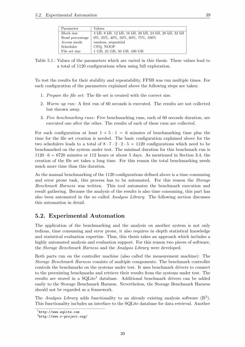
5.2. Experimental Automation 39

Parameter Values

Block size 4 kB, 8 kB, 12 kB, 16 kB, 20 kB, 24 kB, 28 kB, 32 kBRead percentage 0%, 25%, 40%, 50%, 60%, 75%, 100%Access mode random, sequentialScheduler CFQ, NOOPFile set size 1 GB, 25 GB, 50 GB, 100 GB

Table 5.1.: Values of the parameters which are varied in this thesis. These values lead toa total of 1120 configurations when using full exploration.

To test the results for their stability and repeatability, FFSB was run multiple times. Foreach configuration of the parameters explained above the following steps are taken:

1. Prepare the file set : The file set is created with the correct size.

2. Warm–up run: A first run of 60 seconds is executed. The results are not collectedbut thrown away.

3. Five benchmarking runs: Five benchmarking runs, each of 60 seconds duration, areexecuted one after the other. The results of each of these runs are collected.

For each configuration at least 1 + 5 · 1 = 6 minutes of benchmarking time plus thetime for the file set creation is needed. The basic configuration explained above for thetwo schedulers leads to a total of 8 · 7 · 2 · 2 · 5 = 1120 configurations which need to bebenchmarked on the system under test. The minimal duration for this benchmark run is1120 · 6 = 6720 minutes or 112 hours or about 5 days. As mentioned in Section 3.4, thecreation of the file set takes a long time. For this reason the total benchmarking needsmuch more time than this duration.

As the manual benchmarking of the 1120 configurations defined above is a time consumingand error prone task, this process has to be automated. For this reason the StorageBenchmark Harness was written. This tool automates the benchmark execution andresult gathering. Because the analysis of the results is also time consuming, this part hasalso been automated in the so–called Analysis Library. The following section discussesthis automation in detail.

5.2. Experimental Automation

The application of the benchmarking and the analysis on another system is not onlytedious, time consuming and error prone, it also requires in–depth statistical knowledgeand statistical evaluation expertise. Thus, this thesis takes an approach which includes ahighly automated analysis and evaluation support. For this reason two pieces of software,the Storage Benchmark Harness and the Analysis Library were developed.

Both parts run on the controller machine (also called the measurement machine): TheStorage Benchmark Harness consists of multiple components: The benchmark controllercontrols the benchmarks on the systems under test. It uses benchmark drivers to connectto the preexisting benchmarks and retrieve their results from the systems under test. Theresults are stored in a SQLite1 database. Additional benchmark drivers can be addedeasily to the Storage Benchmark Harness. Nevertheless, the Storage Benchmark Harnessshould not be regarded as a framework.

The Analysis Library adds functionality to an already existing analysis software (R2).This functionality includes an interface to the SQLite database for data retrieval. Another

1http://www.sqlite.com2http://www.r-project.org/

39

http://www.sqlite.com

http://www.r-project.org/


Controller Machine

Benchmark Harness

BenchmarkController

Benchmark Driverfor FFSB

Benchmark Driver

Benchmark Driver

Datastore Interface

SQLite Database

R (Analysis Software)

AnalysisLibrary

DatastoreInterface

AggregationFunctions

RegressionFunctions

AnalysisFunctions

System Under Test 2

Machine Hardware

System Under Test 1

Machine Hardware

FFSBBenchmark

Benchmark

Benchmark

SSH

SSH

SSH

Figure 5.1.: Overview of the components involved. Dashed components are existing andtherefore reused. Two additional benchmark have been included in the dia-gram for demonstration purposes. Currently only an FFSB benchmark driveris available. Other benchmark drivers can nevertheless be added easily.

40


Figure 5.2.: Class diagram for the benchmark drivers and the other classes involved in thiscontext.

important functionality of the Analysis Library is the automated model generation. Inthis way, the Analysis Library helps to better understand the benchmark results.

Figure 5.1 gives an overview of the components which were developed for this thesis.Currently the Storage Benchmark Harness only includes a single benchmark driver for theFFSB benchmark. The other two benchmark drivers can be seen as place holders. Inthe following two sections, the two parts of the experimental automation are explained indetail.

5.2.1. Storage Benchmark Harness

The purpose of the Storage Benchmark Harness is the automated execution of bench-marks and the gathering of the results. To interface with a preexisting benchmark onthe system under test, a so–called BenchmarkDriver is used. Figure 5.2 contains anUML class diagram for two example benchmark drivers. As mentioned above only theFFSBenchmarkDriver is currently implemented, the second adapter can be regarded as aplace holder.

As the Storage Benchmark Harness needs an explicit description what experiments shouldbe run on which systems under test, a configuration is necessary. Figure 5.3 shows theUML class diagram for the configuration of the experiments.

Each benchmark driver takes a set of independent variables as input. These independentvariables contain values for each parameter the benchmark driver supports. Additionalvariables are those parameter which are independent from the benchmark but specific forthe system under test, for example the file system. For this reason the FFSBenchmark-

Driver accepts a set of independent variables for the FFSB (IndependentVariablesOf-

41


Figure 5.3.: Class diagram for the classes used to represent the configuration for the bench-marking process.

Parameter Values

fileSystem ext4 XFS

scheduler CFQ

(a) Independent variablespace for system undertest

Parameter Values

readBlockSize 8 kB 16 kB 32 kB

writeBlockSize 64 kB

readPercentage 25% 75%

(b) Independent variable space for benchmark

Table 5.2.: Examples for independent variable spaces.

FFSB) and a set of independent variables specific for the system under test (Independent-VariablesOfSut).

To define multiple experiments at once, the concept of so–called independent variablespaces is used. An independent variable space contains one or more values for each pa-rameter. Using full exploration, an independent variable space can be used to generatemultiple independent variables. Table 5.2 contains two independent variables spaces asexample, one for a system under test and one containing values for the parameters of abenchmark.

An experiment series in this context consists of three parts: The independent variablespace of a system under test, the independent variable space of a benchmark and thesystem where all the experiments should be executed. For example, the two independentvariable spaces given as example above in Table 5.2 can form an experiment series.

As explained above, the independent variable spaces are expanded using full exploration.This means that all possible combinations of the variable values are produced. As anexample, the two independent variable spaces mentioned in Table 5.2 can be expanded

42


Independent Variable Values . . .. . . of System Under Test . . . of BenchmarkfileSystem scheduler readBlockSize writeBlockSize readPrecentage

Experiment 1 ’ext4’ ’CFQ’ 8 kB 64 kB 25Experiment 2 ’ext4’ ’CFQ’ 8 kB 64 kB 75Experiment 3 ’ext4’ ’CFQ’ 16 kB 64 kB 25Experiment 4 ’ext4’ ’CFQ’ 16 kB 64 kB 75Experiment 5 ’ext4’ ’CFQ’ 32 kB 64 kB 25Experiment 6 ’ext4’ ’CFQ’ 32 kB 64 kB 75

Table 5.3.: Example for the full exploration of an experiment series containing the variablespaces defined above in Table 5.2.

Figure 5.4.: Object diagram of a configuration instance.

to the six experiments listed in Table 5.3.

Figure 5.4 contains an UML object diagram for a sample configuration involving twosystems under test which are configured to execute their benchmarks in parallel.

Another important feature of the Storage Benchmark Harness is the synchronized execu-tion of the benchmarks. As explained in the section above, FFSB (and other potentialbenchmarks) run the benchmark in multiple phases. For this reason the benchmark con-troller supports three independent phases which are run for each experiment:

• The preparation phase, where the configuration files can be generated on the systemunder test and the warm–up run can be done. As some benchmarks do not needthis functionality in their benchmark drivers, the implementation is optional. Theimplementation can be done in the prepareExperiment method of the benchmarkdrivers.• The actual benchmarking, where the benchmark is executed and the results are

collected. This happens in the startExperiment method of the benchmark drivers.• A finishing phase, where leftovers can be cleaned up. This is encapsulated in theendExperiment method.

The Storage Benchmark Controller of the Storage Benchmark Harness runs each of thesemethods synchronized on all systems under test. This means that the actual benchmark-ing happens at exactly the same time on all systems under test. This is important forbenchmarking virtualized environments.

43


Figure 5.5.: Class diagram for the runnable parts of the harness which includes the con-troller and the data store.

In a last step, the Storage Benchmark Harness uses a SQLite database to save all theresults to the hard disk. The class diagram in Figure 5.5 shows the runtime componentsof the Storage Benchmark Harness. This also includes the data store interface which isused for the result saving. This enables an analysis of the results independent of thebenchmarking runs by the Analysis Library.

5.2.2. Analysis Library

To analyze the results which are gathered by the Storage Benchmark Harness, R is used.As the storage controller saves the results in a SQLite database, the results must be readfrom there. The Analysis Library additionally contains a set of functions which help tobuild regression models from the results. Additionally, all the analysis done later in thisthesis can automatically be executed. This means that most of the figures and tables inthis thesis can be recreated using new data. Additional analysis on the benchmark resultsor the regression models can be executed using the provided functions and the features ofR.

The automated regression model generation uses the caret library [Kuh08]. Using thislibrary the following steps are done in an automated way:

1. The folding which is needed for the cross–validation (see Section 4.5) is done bysplitting the input data, for which the regression models should be built, into 10folds.

2. For each of the regression techniques which should be evaluated, a cross–validation isexecuted. It uses the folds generate in the step before. Multiple comparison metricsfor each regression technique and each model are stored and recorded. This processensures that all regression models are trained and tested using the same data sets.

3. A final model using all data is generated for each regression technique. This modelis trained using not only 90% of the data as for the cross–validation but using allsamples available.

4. Multiple analyses of the models are prepared and stored for later retrieval. Thisincludes a detailed comparison of the different models including the data necessaryto plot comparison diagrams.

The regression techniques, which are automatically compared by the analysis libraries, canbe configured in detail. This means that additional regression techniques can be included

44


easily. Furthermore the configuration of each of the regression techniques can be providedand is included in the comparison.

By combining the analysis possibilities of R with the functions provided in the AnalysisLibrary, a huge range of analyses can be done. As all the analysis, which was done in thisthesis, is automated, it can easily be repeated for verification purposes or to analyze othersystems or other configurations.

5.2.3. Related Benchmarking Tools

The automated execution of benchmarks and the automated analysis of their results is nota new problem. This means that tools addressing this task have already been developed.This section explains why a new development approach is taken instead of reusing theexisting tools.

Three tools were evaluated for the experimental automation: The Software PerformanceCockpit [WH11, WHHH10], the Ginpex tool [HKHR11] and Faban [Fab]. All three toolswere designed to help the researcher with the benchmarking process. The decision forwriting an own solution and not using and extending one of these tools was made basedupon the following facts.

An important required feature is the automated analysis of the benchmark results, theautomated model generation and the automated analysis of the regression models. Thisfeature is unsupported by all three tools: While the Software Performance Cockpit containsbasic analysis and model generation features, these are designed in an interactive way: Theresearcher can use the user interface to check the results and generate the models. Thesesteps cannot be automated easily. Ginpex does include the visualization of the resultsbut lacks the ability to execute the analysis and the model generation. Faban does notincluded any analysis, it only collects the results and saves them to the researchers harddisk.

All three tools lack the integration of any suitable storage benchmark which has proven tobe the more complex part in the development comparing to the logic which could have beenreused partly from the existing tools. This means that reusing the tools would still haverequired to write the Benchmark Driver for FFSB. Still it is easily possible to integratethis tool in, e.g., the Software Performance Cockpit.

The Software Performance Cockpit provides a framework for benchmark execution andresult analysis. This framework aims at the measurement and modeling of generic soft-ware systems. In contrast to this, the Storage Benchmark Harness provides an domainspecfic approach focused on the performance storage systems. On the technical side, theSoftware Performance Cockpit does not support the execution of benchmarks on multiplehosts, especially not in a synchronized way. Only one host can return results whereasthe other hosts can only act as a load driver. Collecting the results of the benchmarkruns on multiple machines at the same time is an important feature for this thesis. Ad-ditionally, the analysis features of the Software Performance Cockpit are tailored towardsa fast and interactive analysis by the researcher and not towards a fully automated pro-cess. Furthermore, the whole benchmarking and model generation process isn’t automatedin the Software Performance Cockpit. The Software Performance Cockpit also relies onJava Remote Method Invocations (RMI) for the communication between the hosts andthe benchmark tool. This solution requires running Java on the systems under test. Thisintroduces another dependency which might be even impossible to fulfill on some architec-tures where no suitable Java implementation exists. The Software Performance Cockpitcontains multiple features related to the execution of the benchmarks which are not sup-ported by the Storage Benchmark Harness: It supports adaptive benchmarking, where the

45


Metric Metric Metric Metric

Question Question Question

Goal Goal

Defi

nit

ion

Interp

retation

Figure 5.6.: GQM plan schema (based on [BCR94] and [Fab11]).

results are automatically refined to improve the models. Additionally, it supports a muchmore advanced definition of the configuration and parameters.

The Ginpex tool aims in another direction: It helps to generate performance experimentsfrom a model–based specification. This approach was not suitable for this thesis as ex-isting benchmarks had to be reused. On the technical side, Ginpex does not support thecollection of the results of external benchmarks. Only simple metrics, like runtime of thewhole benchmark and the CPU utilization, are supported. As mentioned above, the collec-tion of the results from the benchmark is one of the required features of the tool. Ginpexdoes include the visualization of the results but it provides no regression techniques tobuild prediction models from the collected data. Additionally, Ginpex use RMI in thesame way as the Software Performance Cockpit to communicate with the systems undertest. Ginpex support a sophisticated configuration where many different experiments canbe defined using a high level model. These experiments can involve the benchmarking ofCPU, network and storage performance.

The Faban benchmark harness is a framework focused on the creation and execution ofperformance workloads. As with the other tools, it does not include the features necessaryfor storage benchmarking. On the technical side it does not include a mechanism forrunning multiple experiments described by a single configuration. As mentioned above,Faban does not contain any benchmark result analysis or regression modeling. It does allowthe definition of the benchmark jobs using Java code. This means that the benchmarkjobs are not a static specification but instead can contain logic.

5.3. GQM Plan

The analysis of the benchmark results and the regression models is one of the goals of thisthesis. Another goal is to make the analysis process as repeatable as possible. To simplifynot only the process itself and the interpretation of the results, but also the repeatability,a systematic approach is taken.

The Goal/Question/Metric Approach [BCR94] (short GQM) provides a framework whichhelps to answer research questions in a systematic way. GQM provides two perspectiveson the research progress: For the initial analysis it helps to execute the analysis in amethodical top–down way. For the later interpretation it provides a bottom–up approach.

The main component of GQM is the GQM plan. See Figure 5.6 for the overall structureof a GQM plan. It consists of three layers: The ”goals” layer defines at a conceptual levelthe different objectives. These goals can for example be products, processes or resources.The next level is the operational level. It contains one or more questions for each of the

46

5.3. GQM Plan 47

Goal Question Section

Part I: Experimental Evaluation and Analysis Chapter 6

Evaluation ofMeasurement Setup

How reproducible are the experiments re-sults?

6.1

Evaluation andAnalysis of Parameters

Which parameters have an influence onthe response time?

6.2

What is the influence of virtualization? 6.3

Part II: Performance Modeling Chapter 7

Evaluation andAnalysis of ModelingResults

How good is the interpolation of the re-gression models when using synthetic testsets?

7.1.1

What interpolation abilities do the regres-sion models show when being tested usingnewly collected samples?

7.1.2

How good do the regression models ex-trapolate when using synthetic test sets?

7.1.3

How is the extrapolation ability of the re-gression models when testing using newlycollected data?

7.1.4

How many measurements are needed foran accurate model?

7.1.5

How can the regression modeling of nom-inal scale parameters be improved?

7.1.6

Evaluation andAnalysis of RegressionTechniques

How does the generalization ability of thedifferent regression techniques compare?

7.2.1

What are the advantages and disadvan-tages of the modeling techniques?

7.2.2

Which configuration parameters of the re-gression techniques can improve the pre-diction results?

7.2.3

Table 5.4.: The GQM plan for this thesis with references to the matching sections in thefollowing chapters.

goals. These questions characterize how the goal can be achieved. They specify whichaspects of the object focused in the goal should be approached. At the lowest level, thequantitative level, each question has one ore more metrics. These metrics are used toquantitatively answer the questions and therefore approach the goal. The metrics must bedefined before they are used. Figure 5.6 shows that metrics can be used for two or morequestions if necessary. Often a metric gives insight to more than one aspect of the objectunder research.

The specific GQM plan for this thesis is depicted in Table 5.4. It is grouped into twoparts: The first part discusses the results of the benchmarking in detail. It first checks ifthe measurements setup is suitable. In a next step, the question which parameters have aninfluence on the storage performance is discussed. The second part uses the results from thefirst part and creates regression models based on the benchmark results. These regressionmodels are analyzed in-depth and checked for their generalization abilities. Additionally,alternative approaches to benchmarking and the performance model creation are checked.The second goal of this second part is the evaluation of the regression techniques whichcan be used for generating storage performance models.

47

6. Experimental Evaluation and Analysis

6.1. How reproducible are the experiments results?

This question is of major importance for the interpretation of the results. As each con-figuration is first benchmarked with a warm–up run and afterward with five separatebenchmark runs, the differences of these repetition can be used to answer this question.See Section 5.1 for a detailed view on the benchmarking methodology.

The two metrics which are used to answer this question are the relative error and thestandard deviation of the repetitions. If there is no outer influence and no dependencybetween the repetitions, the standard deviation and the relative error should be zero. Thehigher the standard deviation is, the bigger are the difference between the measurements.These two metrics are applied separately to read and write requests. As explained above,each of the 1120 configurations is repeated five times. These repetitions are executeddirectly after each other. For the calculations in this section, the standard deviationand the relative error of the repetitions mean response time is calculated for each of the1120 configurations: For mean response times of the five repetitions of one configuration,defined as R = {r1, r2, r3, r4, r5}, the standard deviation σR is calculated as explained inSection 4.1.5. The relative error is calculated as follows:

rError =σR · 100%√

5 ·R

This leads to one value for the standard deviation and one value for the relative error foreach of the configurations. These metrics is used to judge on the stability of the singleexperiments in the following paragraphs.

The experiments with the highest standard deviation in their repetitions are depicted inFigure 6.1. The top five standard deviations for the read requests range from 9.8 msto 6.23 ms. The CFQ scheduler generates much more unstable measurements than theNOOP scheduler for read requests. Looking at all experiments which were run using theCFQ scheduler, a mean standard deviation of 2.00 ms is calculated. In contrast to that,those experiments which run on a NOOP scheduler only have a mean standard deviationin their measurements of 1.04 ms. This means that the CFQ scheduler roughly doublesthe standard deviation compared to the NOOP scheduler. It is difficult to identify othersimilarities in the experiments with a high standard deviation.

49

50 6. Experimental Evaluation and Analysis

20

30

40

50

60

70

1 2 3 4 5

Repeat Number

Res

pon

seT

ime

(ms) Dataset

1. CFQ, 100GB fileset, 25% read, rand. access, 8kb blocks


3. CFQ, 75GB fileset, 100% read, seq. access, 28kb blocks

4. NOOP, 50GB fileset, 25% read, rand. access, 8kb blocks


(a) Read Requests

20

30

40

1 2 3 4 5

Repeat Number

Res

pon

seT

ime

(ms) Dataset






(b) Write Requests

Figure 6.1.: Top 5 experiments with the highest standard deviation in the mean responsetime of their repeats.

50

6.1. How reproducible are the experiments results? 51

0

5

10

15

20

25

read write

Rel

ativ

eE

rror

(%)

(a) Boxplot

0.0

0.2

0.4

0.6

0.8

1.0

0 5 10 15 20 25

Relative Error (%)

Cum

ula

tive

Den

sity

Operation

read

write

(b) CDF

Figure 6.2.: Boxplot and cumulative distribution function visualizing the distribution ofthe relative error in the repetition of the experiments.

read (%) write (%)

lower whisker 0.00309 0.00682lower quartile 0.80387 0.56788median 1.98863 1.14751upper quartile 3.77078 2.76742upper whisker 8.02942 6.05783

Table 6.1.: The underlying statistical values for the boxplot in Figure 6.2.

For the write requests the situation is easier to analyze: The NOOP scheduler for hugefile sets and with pure write workload generates the most unstable results. One exceptionis the first experiment which can be regarded as an outlier. The other results show acharacteristic behavior: The response time reduces over the time. This is a clear sign thatthe run time of the benchmark runs is not long enough: The runs are not independentfrom each other. With a warm–up time of two more minutes the results would have beenstabilized. Nevertheless, the question remains why the response time decreases with therepeat number increasing. One would expect that the response time increases due to a fullwrite cache in the storage device after some time. An interesting thing to notice is that forwrite requests the configurations with the highest standard deviation in their repetitionsare those, which do pure write workloads.

For the next examinations, the relative error is used as metric. It is calculated by dividingthe standard deviation by the square root of the repeat count (five in this case) multipliedby the mean of the repeats. This allows to judge on the deviation of the results in arelative way. Figure 6.2 contains two boxplots and a CDF which show the distribution ofthe relative errors for both read and write requests. The underlying data can be found inTable 6.1.

For the write requests, the maximum relative error is 14.4% which is an acceptable value,especially under the conditions the measurements were retrieved. Those measurementswith a huge relative error within their repetitions show the same characteristics as theworst measurements using the standard deviation: The response time gets better over thefirst 3 repeats and then stabilizes.

51


For the read requests the highest relative error is 25.5%. This is a much bigger numberwhich leads to the assumption that read requests are much more unstable than writerequests. This assumption can be backed up by the fact that the read cache of the DS8700is much larger than the write cache. The mean relative error of all measurements does notshow this difference: It is 3.34% for read requests and 2.10% for write requests.

To summarize this answer: The repetitions are not as stable as they are desirable. Itis not clear why this is the case. Due to the complex nature of the storage system andthe unavailability of analysis tools, the cause of these effects remain unknown. A longermeasurement time per repetition would increase the stability. Instead of benchmarkingfor five times one minute it would be necessary to benchmark five times five minutes.Additionally an increase in the warm–up time is necessary, especially for the write requests.This was unfeasible due to time constraints: This increase of the benchmarking time wouldalso increase the total benchmarking duration. With a benchmarking time of already morethan one week a further increase is not feasible. It is still possible to use the current resultsas if only a single run of five minutes was run. This can be done easily by calculating themean of all five repetitions and treating this value like a single repeat. Nevertheless, therepetitions are needed for the analysis of the parameters influence in the next section.

6.2. Which parameters have an influence on the responsetime?

The answers to this question plays an important role on the choice on the parameters whichshould be benchmarked in detail. Additionally, the answer to this question helps to decidewhich parameters should be included in the models later in Chapter 7. If the answer to thisquestion concludes that some parameters have no influence on the storage performance,these parameters could be left out of the model generation and further benchmarking.

An ANOVA of the parameters is the typical way to solve this problem and the results of theANOVA are used as metric to answer this question. Section 4.2 contains an explanationhow to interpret the results of an ANOVA analysis. To execute this ANOVA, the meanof each benchmark run was calculated separately for read and write requests. For both,the read and write requests, two separate ANOVAs were executed. Table 6.2 show theresults of these analyses separately for read and write requests. As the probability thateach parameter has no influence on the result is nearly zero (the exact value is smallerthan 2−16) for all parameters, it can be assumed that all five parameters influence thevariation of the mean response time. This is true for both, read and write requests.Figure 6.3 contains a graphical representation for the quantification of the influence of theparameters on the variation. This quantification show a huge impact of the scheduler.This is a logical result as the CFQ scheduler is somehow unsuited for the IBM DS8700with its sophisticated caching mechanisms. Another point is the huge relative influenceof the residuals. These residuals can either result from measurement errors or can simplybe those parts of the variation which cannot be explained using the supplied parameters.Later in this section it becomes clear that the second case is true: The measurement errordoes in fact not have such a huge influence on the variation. In this context this onlymeans that only about 55% of the variation can be explained using the five parametersand all the other variation is counted towards the residuals. An interesting differencebetween the read and the write requests is the influence of sequential and random access.For read requests this does not have a huge influence while for write requests changingfrom sequential to random access affects the response time.

In the following paragraph, it is checked that not only the simple parameters influencethe response time but also their interactions. To verify this assumption, an ANOVA test

52

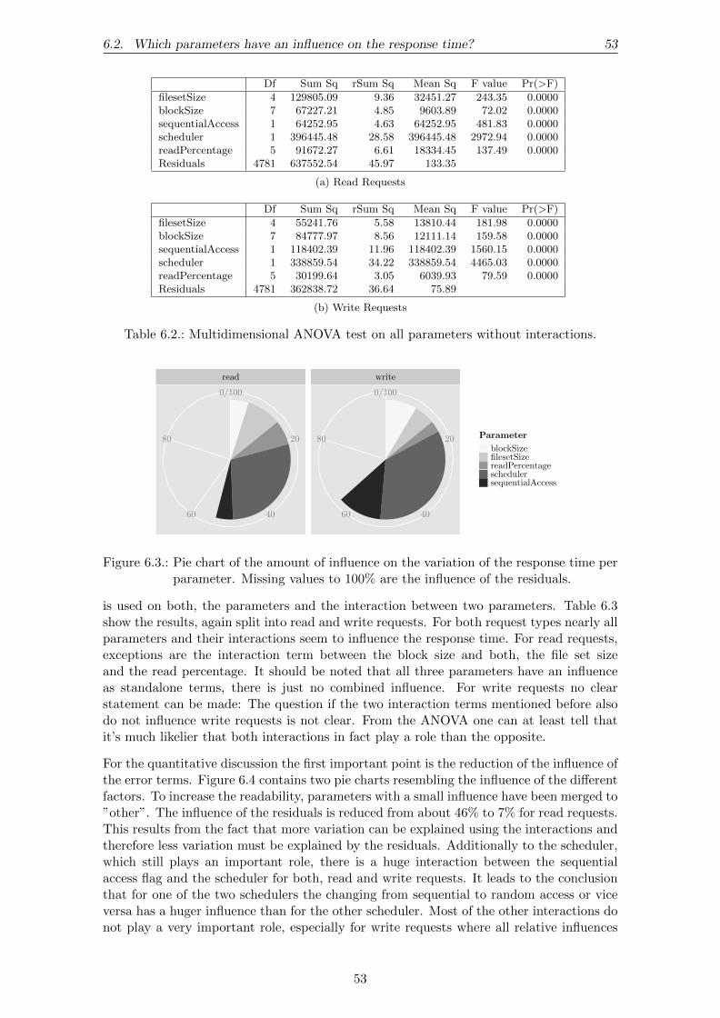
6.2. Which parameters have an influence on the response time? 53


filesetSize 4 129805.09 9.36 32451.27 243.35 0.0000blockSize 7 67227.21 4.85 9603.89 72.02 0.0000sequentialAccess 1 64252.95 4.63 64252.95 481.83 0.0000scheduler 1 396445.48 28.58 396445.48 2972.94 0.0000readPercentage 5 91672.27 6.61 18334.45 137.49 0.0000Residuals 4781 637552.54 45.97 133.35

(a) Read Requests


filesetSize 4 55241.76 5.58 13810.44 181.98 0.0000blockSize 7 84777.97 8.56 12111.14 159.58 0.0000sequentialAccess 1 118402.39 11.96 118402.39 1560.15 0.0000scheduler 1 338859.54 34.22 338859.54 4465.03 0.0000readPercentage 5 30199.64 3.05 6039.93 79.59 0.0000Residuals 4781 362838.72 36.64 75.89

(b) Write Requests

Table 6.2.: Multidimensional ANOVA test on all parameters without interactions.

read write

20

4060

80

0/100

20

4060

80

0/100

Parameter

blockSizefilesetSizereadPercentageschedulersequentialAccess

Figure 6.3.: Pie chart of the amount of influence on the variation of the response time perparameter. Missing values to 100% are the influence of the residuals.

is used on both, the parameters and the interaction between two parameters. Table 6.3show the results, again split into read and write requests. For both request types nearly allparameters and their interactions seem to influence the response time. For read requests,exceptions are the interaction term between the block size and both, the file set sizeand the read percentage. It should be noted that all three parameters have an influenceas standalone terms, there is just no combined influence. For write requests no clearstatement can be made: The question if the two interaction terms mentioned before alsodo not influence write requests is not clear. From the ANOVA one can at least tell thatit’s much likelier that both interactions in fact play a role than the opposite.

For the quantitative discussion the first important point is the reduction of the influence ofthe error terms. Figure 6.4 contains two pie charts resembling the influence of the differentfactors. To increase the readability, parameters with a small influence have been merged to”other”. The influence of the residuals is reduced from about 46% to 7% for read requests.This results from the fact that more variation can be explained using the interactions andtherefore less variation must be explained by the residuals. Additionally to the scheduler,which still plays an important role, there is a huge interaction between the sequentialaccess flag and the scheduler for both, read and write requests. It leads to the conclusionthat for one of the two schedulers the changing from sequential to random access or viceversa has a huger influence than for the other scheduler. Most of the other interactions donot play a very important role, especially for write requests where all relative influences

53



filesetSize 4 129805.09 9.36 32451.27 1470.20 0.0000blockSize 7 67227.21 4.85 9603.89 435.10 0.0000sequentialAccess 1 64252.95 4.63 64252.95 2910.98 0.0000scheduler 1 396445.48 28.58 396445.48 17960.94 0.0000readPercentage 5 91672.27 6.61 18334.45 830.64 0.0000filesetSize:blockSize 28 300.09 0.02 10.72 0.49 0.9897filesetSize:sequentialAccess 4 48776.42 3.52 12194.10 552.45 0.0000filesetSize:scheduler 4 7805.86 0.56 1951.47 88.41 0.0000filesetSize:readPercentage 20 4569.28 0.33 228.46 10.35 0.0000blockSize:sequentialAccess 7 43219.46 3.12 6174.21 279.72 0.0000blockSize:scheduler 7 15613.25 1.13 2230.46 101.05 0.0000blockSize:readPercentage 35 608.33 0.04 17.38 0.79 0.8100sequentialAccess:scheduler 1 388654.37 28.02 388654.37 17607.97 0.0000sequentialAccess:readPercentage 5 23591.17 1.70 4718.23 213.76 0.0000scheduler:readPercentage 5 1445.42 0.10 289.08 13.10 0.0000Residuals 4665 102968.87 7.42 22.07

(a) Read Requests



(b) Write Requests

Table 6.3.: Multidimensional ANOVA test on all parameters including interaction termsbetween two parameters.

read write

20

4060

80

0/100

20

4060

80

0/100

Parameter

blockSizefilesetSizeotherreadPercentageschedulersequentialAccesssequentialAccess:scheduler

Figure 6.4.: Pie chart of the amount of influence on the variation of the response time perparameter. It includes interactions between two parameters. Values smallerthan 5% have been aggregated to ”other”. Missing values to 100% are theinfluence of the residuals.

54

6.2. Which parameters have an influence on the response time? 55

are below 4%.

Including a higher level of interaction in the ANOVA has not proven to be of much value:None of the interaction terms has more than 3% influence on the variation. Additionally,the ANOVA table gets large and more difficult to read. Nevertheless, it should be notedthat the amount of variation that cannot be explained using the parameters and theirinteractions goes down to 1.29% for read requests and 0.47% for write request. Theresults from the two ANOVAs can be found in Appendix A.

The input for these four ANOVAs are the 1120 configurations which were repeatedlybenchmarked five times. This leads to a total of 5600 measurements which are analyzed.A possiblity to reduce the number of measurements required is to limit each parameteronly to its extremes. This means that for each parameter only two values are benchmarked,its minimum and its maximum. This is called a n2m ANOVA [Kou11] because only n2m

measurements are needed where n is the number of repetitions and m the number ofparameters. In the case of this thesis this would lead to 160 measurements, only about3 percent of the measurements needed for a full exploration. The question arises if thesereduced sets is still sufficient to check which parameters have an influence on the responsetime. To analyze this, a subset of the existing measurements is built containing only theextreme values. This means that the following values are included:

• Block size: The two extreme values 4 kB and 32 kB are included.• File set size: Again the minimum and the maximum of 1 GB and 100 GB are the

only file set sizes which are included in the subset.• Read percentage: For the read percentage it is not possible to simply select the lowest

and the highest read percentage to be included in the subset. The reason for thisis that a read percentage of 0% would lead to no read request issued and thereforeno result would be recorded. The same is true for a read percentage of 100% andwrite requests. For this reason the values included for the read percentage are 25%and 75%, the second lowest and second highest values which were benchmarked. Fora future benchmarks, values closer to the minimum and maximum might lead tobetter results.• Scheduler and sequential access are left unmodified as they already include only two

values.

Table 6.4 contains the results of two separate ANOVAs executed on the reduced sampleset specified above. Again a separate ANOVA is done for read and write requests. Byreducing the samples, the results of the ANOVA got much more insecure. For multipleinteraction terms the answer to the question whether they influence the mean responsetime or not cannot be answered with a high reliability. For example the interaction termbetween file size and scheduler has a five percent probability to have no influence on theresponse time. In contrast to that, in the full factorial ANOVA it can be assumed with avery high probability that there is in fact an influence. On the other side for example theinteraction term between file set size and block size also has a probability of five percent tohave no influence. As stated above this is in fact true, the full ANOVA has a probabilityof 99% for this term. These two examples show that a five percent probability of influencefor a n2m ANOVA can result in a very high probability and a very low probability in a fullfactorial ANOVA. Therefore the reduction of the parameter values does not pay out. Thequantitative analysis shows that the values are a rough estimate for the values of a fullfactorial ANOVA. The top four influencing factor are the same for both methods. Afterthis the results diverge with makes an analysis of the less important factors impossible.

The overall answer to this question is: All of the five evaluated parameters and nearlyall interactions between two parameters have an influence on the response time. The

55




(a) Read Requests



(b) Write Requests

Table 6.4.: Multidimensional ANOVA test on all parameters including interactions be-tween two parameters. Only two values were included for each parameter,leading to a n2m ANOVA and a reduction of the required benchmark runs.

56

6.3. What is the influence of virtualization? 57

read (%) write (%)

lower whisker 0.00071 0.00485lower quartile 4.27833 5.05743median 8.53218 10.41316upper quartile 14.45540 26.06969upper whisker 29.14669 51.32413mean 10.60307 16.67317

Table 6.5.: Underlying data for the boxplot in Figure 6.5.

reduction of the values when going from full factorial to a n2m experimental design cannotbe supported due to ambiguous results.

6.3. What is the influence of virtualization?

As the IBM System z is a virtualized machine and as virtualization has become an im-portant technology, the question arises if the influence of virtualization can be capturedby the measurements. To check this, the measurements, which were gathered previously,are compared to newly run benchmarks with the same I/O load distributed on two virtualmachines. The comparison was done using the relative error as metric.

As the NOOP scheduler shows a much more stable results, this examination is limited tothis scheduler. The CFQ scheduler is left out intentionally. The 560 remaining configura-tions explained above, are all benchmarked using 100 threads. To check if the benchmark-ing process can be used even if multiple virtual machines are involved, new benchmarkconfigurations are created: 560 new configurations are defined using only 50 threads, ex-actly half of the original 100 threads. Additionally the file set is also halved which meansthat the following file set sizes are benchmarked: 500 MB, 12.5 GB, 25 GB, 37.5 GB,50 GB. For each of these 560 configurations two identical benchmark runs are started si-multaneously on two virtual machines. The virtual machines are configured identically tothe machine where the original benchmarks were run. The simultaneous execution of thebenchmark is fully automated using the Storage Benchmark Harness which was developedfor this thesis.

By using this setup, the load which is generated by the benchmarks should be identical inthe one virtual machine case and the two virtual machine case. Three results exists perconfiguration: The result from the original run on a single virtual machine and the resultsfrom the two virtual machines when running in parallel. Under ideal conditions, one canexpect that the mean response times of all three benchmark runs are identical. To checkif this assumption is true, the relative error is calculated as following:

rError =

∣∣∣∣∣ dualVM1+dualVM22 − singleVM

singleVM

∣∣∣∣∣In this definition, ”singleVM” is the mean response time of the requests when running on asingle virtual machine. These are the results from the original measurements. ”dualVM1”and ”dualVM2” are the mean response time gathered when the benchmark was run ontwo virtual machines simultaneously. This definition means that the mean of the resultsof the dual virtual machine case is compared to the single virtual machine case using therelative error. The ”singleVM” variable contains the results from the configuration wherethe thread count and the file set size was doubled comparing to the configuration whichwas used when obtaining the ”dualVM1” and ”dualVM2” data. The read and the writerequests are aggregated separately because of their different behavior.

57


0

20

40

60

read write

Rel

ativ

eE

rror

(%)

(a) Boxplot

0.0

0.2

0.4

0.6

0.8

1.0

0 20 40 60

Relative Error (%)

Cum

ula

tive

Den

sity

Operation

read

write

(b) CDF

Figure 6.5.: Boxplots and CDF for the relative errors of the read and the write requests.The relative error between the case when running the benchmark on twoseparate virtual machines and the case when running a single benchmark ona single virtual machine is depicted here.

Figure 6.5 shows the results of this analysis: The relative errors of all configurations wasincluded in the two boxplots and in the CFD: One boxplots contains the relative errors ofthe read requests and one boxplot contains the relative errors of the write requests. Themean is 10.6% for read requests and 16.6% for write requests. This can be regarded asgood values, although these number suggest that the assumption made above cannot befully supported. When looking at the boxplot more detailed, a different behavior betweenread and write requests can be shown: For the read requests, 50% of the configurationshave a relative error in the quite narrow range between 4.2% to 14.4%. This also meansthat the outliers, which have their maximum at 67.1%, contribute a lot to the high meanrelative error. When looking at the CDF, it becomes clear, that about 80% of the sampleshave a relative error below 18%. Later in this section, the reasons for this behavior areanalyzed.

When looking at write requests, the 50% interval is between 5.0% and 26.0%. This meansthat, compared to the read requests, the majority of the configurations have a huge varia-tions in their relative errors. Based on the numbers, one can conclude that the assumptionmade above does only hold in a restricted way for write requests.

The question where these high relative errors results from is discussed next. To analyzethis, the configurations are split according to their read percentage. The results can befound in Figure 6.6. For the read requests, depicted in the upper part of the diagram, the0% read percentage has no boxplot. The reason for this is, that with a read percentage of0%, no read requests were issued and therefore no relative error could be calculated. Forthe same reason there is no boxplot for the 100% read percentage and write requests.

When looking at the read requests, it becomes clear that for pure workloads, the relativeerror is very low. Pure workloads are workloads with only read or only write requests. For

58

6.3. What is the influence of virtualization? 59

0

20

40

60

0

20

40

60

read

write

0 25 40 50 60 75 100

Read Percentage (%)

Rel

ativ

eE

rror

(%)

Figure 6.6.: Boxplots comparing the relative errors depending on the read percentage. Theread percentage is the amount of operations which are read requests.

59


the read requests, the mean relative error for pure read workloads is 2.8% which is a verygood value. When decreasing the read percentage and therefore increasing the amount ofwrite requests issued, the mean relative error and its variation increase significantly.

For write requests, the relative error is also quite low for a pure write workload: The meanrelative error for the configuration with a read percentage of 0% is 6.0% and the variationis quite small. In contrast to the read requests the error and especially the variation goesup very fast when increasing the read percentage.

Although the configurations were chosen to produce the same I/O load on the system intotal, the results are not clear: It can be concluded from the numbers and figures presentedabove that this assumption can only be fully supported for pure workloads. For all otherworkloads, especially for write requests, the relative error is too high.

60

7. Performance Modeling

7.1. Evaluation and Analysis of Modeling Results

One of the major tasks of this thesis is the generation of storage performance predictionmodels. As the generation is fully automated, the question of the quality of the modelscan be discussed in detail. The following sections discuss the question of interpolation andextrapolation of the regression models.

The models, whose quality is analyzed in the following sections, are generated based on the1120 configurations defined in Section 5.1. Each of these configurations is benchmarkedfive times. The mean of the mean response time of all repetitions is recorded for eachconfiguration. This leads to a total of 1120 samples for the regression model creation. Therepetitions are not used separately but aggregated because of the short benchmarking timeand huge differences in the repetitions as discussed in Section 6.1. If longer measurementsare available it would be possible to include these repetitions in the modeling process.Two separate models are generated for read and write requests. This is done because readand write requests have a completely different behavior and different characteristics.

Four different regression techniques are used to generate nine regression models. An uniqueidentifier is given to each of these nine models for referencing purposes.

• Linear Regression (as explained in Section 4.3.1):

– lm: A linear model is trained using only the five input parameters. Multipleauthors state that this regression technique is inappropriate for modeling stor-age performance. For this reason no sufficient model quality can be expected.The model is nevertheless included for comparison reasons and to prove theassumptions which have been made during the discussion of the influence ofthe parameters in Section 6.2.

– lm 2param inter: This linear model contains the five input parameters andalso the ten interaction terms between pairs of two parameters. This leads to atotal of 15 coefficients which have to be computed. This enables the model toadapt to interactions between two parameters.

– lm 3param inter: This model additionally contains the interaction terms be-tween three of the parameters. There are 10 of these terms. This leads to atotal number of 5 + 10 + 10 = 25 terms in the model. This setting allows themodel to additionally include interactions between three parameters.

61

62 7. Performance Modeling

– lm 4param inter: Similar to above, this model contains the interactions be-tween up to four parameters. There are five of these interaction terms whichleads to a total number of 5+10+10+5 = 30 terms in the model. The inclusionof the interactions allows the model to even model interactions between fourparameters.

– lm 5param inter: This model includes everything of the above model plus asingle term modeling the interactions between all five parameters. For thisreason the total number of terms is 5 + 10 + 10 + 5 + 1 = 31 terms. This is thehighest number of terms possible for five parameters.

• Multivariate Regression Splines (as explained in Section 4.3.2 for the statistical back-ground):

– mars: This MARS model was trained allowing no interaction terms. This meansthat the degree parameter of the MARS algorithm was set to 1. This makesthis model comparable to the lm model above which also does not containinteraction terms.

– mars multi: For this MARS model the degree parameter was set to a value offive. This extension allows the MARS algorithm to choose interaction termsbetween up to five parameters. This extends the list of possible terms but doesnot mean that these term are necessarily included in the final model. Thissetting allows the MARS model to include the same interaction terms as thelm 5param inter linear regression model. For the MARS algorithm this settingallows to choose the actual terms for all interaction terms, including those usingtwo, three, four, and five parameters.

• Regression Tree (as explained in Section 4.3.3 for background information) cart: Aregression tree is trained on the data using the cart algorithm.

• M5 (as explained in Section 4.3.4 for detailed explanation) m5: An M5 regressiontree with attached linear models trained using the training samples.

All other configuration parameters of the regression techniques are set to their implemen-tation defaults. In Section 7.2.3 these configuration parameters are further examined.

All regression techniques except CART are not designed for non interval scales. Some ofthe parameters discussed in this thesis are on a nominal scale. This includes the schedulerand the sequential/random access flag. To model these nominal parameters, a classifica-tion model would be a better choice. The problem here is that classification models donot support interval scales. For this reason the nominal parameters are transformed to aninterval scale by assigning integer values to each level. For the sequential/random accessflag a new parameter ”sequentialAccess” is created. It has the value ”0” for sequentialaccess and ”1” for random access. The scheduler parameter is transformed into a ”sched-ulerNOOP” parameter. This parameter is ”1” if the scheduler is NOOP and ”0” if thescheduler is CFQ. This approach can be extended to more values, for example if a thirdscheduler had been benchmarked.

The quality of the models can only be judged using samples which were not used in thetraining process (see Section 4.5 for the reasons). The samples which were not used arecalled the training set. By calculating the predictions of the models for this training setand then comparing the predicted with the actual values the model quality can be judged.For this process different metrics are used: The root mean square error (RMSE) and themedium absolute percentage error (MAPE). For their differences see Section 4.4. By usingthese metrics, the quality of the models is an indication for the generalization ability. The

62

7.1. Evaluation and Analysis of Modeling Results 63

Read Model Write ModelModel RMSE MAPE RMSE MAPE

(ms) (%) (ms) (%)

lm 11.51 87.02 8.77 66.32lm 2param inter 4.80 31.40 3.26 18.12lm 3param inter 3.13 16.72 2.62 10.35lm 4param inter 2.95 13.43 2.56 9.26lm 5param inter 2.96 13.47 2.56 9.19cart 6.16 38.40 5.20 38.11mars 11.54 86.36 8.75 66.84mars multi 4.86 34.34 2.86 16.00m5 1.69 6.49 0.81 4.24

Table 7.1.: Underlying data for the boxplots in Figure 7.1, which show the comparison ofthe interpolation abilities of the regression models when tested using 10-foldcross–validation.

generalization ability is split into two parts: The generalization ability within the modeledranges, the so–called interpolation and out of the ranges, the so–called extrapolation.

The results of the following sections are later summarized in Section 7.1.7.

7.1.1. How good is the interpolation of the regression models when usingsynthetic test sets?

To check how good the regression models interpolate, the 1120 input samples are dividedinto two groups: 90% of the data is used to train the model and 10% of the data is usedto check how good the model generalizes. Ten of these training–test pairs are generated.Then each model specified above is trained using the ten training sets and tested usingthe ten test sets. RMSE and MAPE are used as metrics. This leads to ten values for bothmodel metrics for each of the nine models. This process assures, that for comparabilityreasons, each model is trained using exactly the same training data. Although the goalsseem to be different, this approach is the same as 10-fold cross–validation (see Section 4.5for an explanation). This process is needed because the naive approach, to build a modelusing the whole data set and then take some test samples out of this set to check themodels quality, is not an acceptable way. As explained before, this process would notdetect an overfitted model.

Figure 7.1 contains boxplots for each model and each metric. As there were separatemodels for read and write operations, two boxplots exist for each model and each metric.Both metrics produce smaller values if the model is better. Each boxplot includes theresults of the ten validation runs. When comparing the models, the mean of the ten cross–validation runs is used. The mean is depicted as a white dot in the box plots. Table 7.1contains the underlying data.

Although the definitions of the metrics differ, they lead to the same order in the models.Both metrics clearly identify the M5 model as the model with the best generalizationability. The M5 model (m5) performs very well: For the read model, the mean absolutepercentage error (MAPE) is 6.49% and 4.24% for the write model. This means that theaverage prediction error is 6.49% or 4.24%. The root mean square error (RMSE) is 2.96 msfor the read model and 0.81 ms for the write model. These results are very good, especiallywhen considering the complexity of the system. The M5 model is able to adapt very wellto the test data and generalize.

The second best model is the linear regression model which includes all interactions upto five parameters (lm 5param inter): With a MAPE of 13.47% and 9.19% for read andwrite models and an RMSE of 2.96 ms and 2.56 ms respectively, it performs significantly

63


m5

mars multi

mars

cart

lm 5param inter

lm 4param inter

lm 3param inter

lm 2param inter

lm

m5

mars multi

mars

cart

lm 5param inter

lm 4param inter

lm 3param inter

lm 2param inter

lm

read

write

2 4 6 8 10 12

(a) RMSE in ms

m5

mars multi

mars

cart

lm 5param inter

lm 4param inter

lm 3param inter

lm 2param inter

lm

m5

mars multi

mars

cart

lm 5param inter

lm 4param inter

lm 3param inter

lm 2param inter

lm

read

write

0 20 40 60 80 100

(b) MAPE in %

Figure 7.1.: Comparison of the quality of models generated using the full data set. Twodifferent metrics were used: Root Mean Square Error (RMSE) and MediumAbsolute Percentage error (MAPE).

64


worse than the M5 model. Nevertheless these results are also very good, especially whenkeeping the simple nature of the linear regression models in mind. It is interesting tosee that a linear regression is sufficient for adapting to the rough structure of the storageperformance data.

The inclusion of the single interaction term which consists of all parameters in the lm -

5param inter model does not provide a significant improvement. The lm 4param inter

model which does not include this term has only a 0.04% (read model) or 0.07% (writemodel) lower MAPE and a 0.01 ms (read model) or 0.003 ms (write model) lower RMSE.The differences are so small that one can conclude that the interaction between all fiveparameters does not play a role when predicting the storage performance.

It might seem surprising that more sophisticated techniques like MARS or CART did notperform better: The MAPE of the multidimensional MARS model, which can include thesame interaction terms as the lm 5param inter, has a MAPE of 34.34% and 16.00% whichis about the double value of the linear model and more than four times the value of theM5 model. The values them–selves are not very good but could be acceptable, dependingon the use case of the models. They can be used for a rough estimate. The reason for thisbehavior is discussed later in Section 7.2.1 where the modeling techniques are compared.

When comparing read and write models, the write model are better for all modelingtechniques. This results from the benchmark results: They are more stable and easier topredict for write requests. The reason for this behavior is mainly the smaller cache forwrite requests compared to the cache for read requests: The write cache is only 2 GB insize, whereas the read cache is 50 GB large.

In general the models perform very good. It must be kept in mind that a complex storagesystem with many layers is modeled. A MAPE of 6.49% is acceptable for most uses of themodel. Later in Section 7.2.2 a detailed comparison between the different model techniquesis done.

7.1.2. What interpolation abilities do the regression models show whenbeing tested using newly collected samples?

While the previous question analyzes the interpolation abilities of the regression modelsusing a synthetic test set generated from the existing samples, this section takes anotherapproach: It uses newly collected benchmark results.

For this section the whole 1120 samples are used to train the nine models. This is a slightincrease in the training samples: In the previous section, the models are trained using1108 samples (90% of 1120), this time the whole 1120 samples are used. To verify theinterpolation abilities of these models, new samples are collected. The configurations ofthese samples are composed as follows:

• The block size is randomly selected from the range 4 kB to 32 kB.

• The read percentage is randomly selected from the range 0% to 100%.

• The file set size is taken randomly from the range of 1 GB to 100 GB.

• The sequential access flag is randomly chosen between random access and sequentialaccess.

• The scheduler is randomly chosen out of the two available schedulers NOOP andCFQ.

All other benchmark settings remain at the same values which are used to obtain theoriginal results. As the FFSB benchmark only supports block sizes which are a multiple

65



(ms) (%) (ms) (%)


Table 7.2.: Comparison of the interpolation abilities when using 200 newly collected ran-dom samples. This is the underlying data for the bar plots in Figure 7.2.

of 512 bytes the block sizes are rounded to the nearest 512 byte step. Because the file setis composed out of files with a size of 16 MB, the file set size is rounded to the nearest16 MB step. All other values are left at their randomly selected values. This means thatfile set size and read percentage can take any value in the mentioned range. No roundingis done.

This approach randomly selects configuration within the benchmarked range to test theinterpolation of the models. 200 configurations are randomly composed out of the speci-fication above. Each of these configurations is benchmarked in five runs each lasting forone minute. The results of the five runs are averaged. The approach of benchmarking newsamples can be regarded as more realistic compared to the previous section: It simulatesthe later use of the models where other values than those benchmarked are predicted usingthe models.

Figure 7.2 and Table 7.2 contain the results for this interpolation test. The results are verypromising: The samples are collected purely randomly and it was unclear what behavior,for example, a randomly selected block size has on the results. The M5 model againperforms very well: The RMSE is 3.56 ms for the read model and 2.44 ms for the writemodel. The MAPE is 9.27% and 10.39% respectively. When compared to the previoussection these results are worse because of the random gathering of the results.

When looking at the linear regression with all interaction terms the MAPE is 13.87% and10.01% for the read and the write models. The RMSE is 4.81 ms and 2.60 ms respectively.These are very good values which are only slightly worse than those of the synthetic testin the section before.

When regarding the multidimensional MARS model, the values are 6.49 ms and 2.84 msfor the RMSE and 28.52% and 16.64% for the MAPE. Like in the section before, thesevalues are too high to be regarded a good fit.

The experiment conducted here shows more expressiveness than the one in the sectionbefore. Both sections show that the linear regression model containing all interactionterms and the M5 model have an acceptably low error for both, read and write models.One can conclude that the interpolation ability of the models is good. As the interpolationis one of the most important features, this first major result of the thesis is very promising.

In the next section, the discussion is extended to those values which are out of the rangeof the parameters. This means that the extrapolation abilities of the models are checked.

66


m5

mars multi

mars

cart

lm 5param inter

lm 4param inter

lm 3param inter

lm 2param inter

lm

m5

mars multi

mars

cart

lm 5param inter

lm 4param inter

lm 3param inter

lm 2param inter

lm

read

write

0 5 10

(a) RMSE in ms

m5

mars multi

mars

cart

lm 5param inter

lm 4param inter

lm 3param inter

lm 2param inter

lm

m5

mars multi

mars

cart

lm 5param inter

lm 4param inter

lm 3param inter

lm 2param inter

lm

read

write

0 20 40 60 80

(b) MAPE in %

Figure 7.2.: Comparison of the interpolation abilities of the nine regression models testedusing 200 newly collected randomly selected samples.

67



(ms) (%) (ms) (%)


Table 7.3.: Comparison of the extrapolation abilities when reducing the original sample setby removing the extreme values and reuse the removed samples for training.This is the underlying data for the bar plots in Figure 7.3.

7.1.3. How good do the regression models extrapolate when using syn-thetic test sets?

This question discusses the quality of the predictions out of the modeled range. This playsan important role, because not all possible configurations can be benchmarked beforehand.Again, the metrics for this question are RMSE and MAPE. Because some parametershave a closed range, extrapolation does not make sense for those parameters: The readpercentage is already benchmarked from 0 to 100% and obviously no predictions out ofthis range can be made. The sequential/random access flag cannot be extended to morevalues. The prediction of values for other schedulers out of the existing data is not feasible.For the five parameters which are analyzed in this thesis the file set size and the block sizeare the only two parameters where extrapolation is an issue.

To test the extrapolation abilities of the models, this section takes a synthetic approachwhich solely relies on the already collected samples. In contrast to this, the next sectionjudges on the extrapolation using newly collected samples. The advantage of this approachis that no new samples have to be collected. As the benchmarking of new configurationsis time consuming, judging on the extrapolation without gathering new results can be adesirable option.

All configurations which meet one of the following four conditions are removed from thesample set:

• The block size is 4 kB.• The block size is 32 kB.• The file set size is 1 GB.• The file set size is 100 GB.

This procedure removes the extreme values for both, block size and file set size from thesample set. 616 of the 1120 samples are removed. This leads to a remaining sample setof 504 elements. The reduced data set is then used to train the nine regression modelsdefined above. The regression models which were built using the reduced data set werethen tested. The test data consists of 100 randomly selected samples which were drawnout of the 616 samples which were removed in the initial step. This approach reduces thetraining set to get the possibility to test using the extreme values and therefore judge onthe extrapolation abilities of the models. The disadvantage of this approach is that only504 samples were available for the model creation. Especially for regression techniqueswhich need a lot of data to fit the model, the results are not expected to be very good.

68


m5

mars multi

mars

cart

lm 5param inter

lm 4param inter

lm 3param inter

lm 2param inter

lm

m5

mars multi

mars

cart

lm 5param inter

lm 4param inter

lm 3param inter

lm 2param inter

lm

read

write

0 2 4 6 8 10

(a) RMSE in ms

m5

mars multi

mars

cart

lm 5param inter

lm 4param inter

lm 3param inter

lm 2param inter

lm

m5

mars multi

mars

cart

lm 5param inter

lm 4param inter

lm 3param inter

lm 2param inter

lm

read

write

0 20 40 60 80 100

(b) MAPE in %

Figure 7.3.: Extrapolation abilities of the regression models, trained using a reduced dataset and tested using the left out samples.

69


The four bar charts in Figure 7.3 and the Table 7.3 show the results of this test. Theoverall results from this approach are very good considering the conditions under whichthe models have been generated.

The M5 model again performs the best: The MAPE is 15.67% for the read model and20.99% for the write model. The RMSE is 2.96 ms and 4.91 ms respectively. In contrastto the previous section, this time the read model performs better than the write model.The write model suffers more from the reduction of the training set.

For the linear model containing all interactions possible (lm 5param inter), the RMSEis 3.67 ms for the read model and 4.76 ms for the write model. The MAPE is 23.22%and 21.32% respectively. Again the write model does not perform better than the readmodel as observed in the section before. The advantage of M5 compared with the linearregression model gets smaller if the training set is reduced. For the write models, theRMSE of the linear regression model is even lower than the RMSE of the M5 model.

One can expect a better extrapolation if the model is built using the full sample set andadditional values which are out of the range of this original sample set are used to test themodel. This approach is taken in the next question.

7.1.4. How is the extrapolation ability of the regression models whentesting using newly collected data?

This section focuses on another approach on how to measure the extrapolation abilitiesof the regression models. In contrast to the question before, where the existing datais used to judge on the extrapolation abilities, this section focuses on the more naturalapproach: New measurements are obtained and used to test the model. As in the previoussections, the metrics are RMSE and MAPE. The metrics are calculated based on thenewly generated test samples.

This approach leads to the fact that the whole 1120 samples which are described in Sec-tion 5.1 are used to train the nine regression models. To test the extrapolation, newlycollected benchmark results are used: The new experiments are randomly generated usingthe following schema:

• Block size: The block size is randomly chosen out of the following set: 1 kB, 2 kB,36 kB, 40 kB, 48 kB and 64 kB. These values are chosen because they are not includedin the original block size range which has its minimum at 4 kB and its maximum at32 kB.

• File set size: The file set size is also randomly sampled using the following set:256 MB, 512 MB, 110 GB and 130 GB. The original range of the file set size is1 GB to 100 GB. Values larger than 130 GB can not be benchmarked due to sizeconstraints: The benchmarked storage volume cannot hold more than 130 GB ofdata.

• Scheduler : Random selection of either CFQ or NOOP scheduler.

• Read percentage: The same value as in the original experiments: From 0% to 100%in seven steps.

• Sequential access: Both, random and sequential access were benchmarked.

This schema uses the original values for all parameters except for the block size and thefile set size. Out of these 6 · 4 · 2 · 7 · 2 = 672 possible configurations, 200 configurationsare randomly selected as test set. This test set is benchmarked running for five times

70



(ms) (%) (ms) (%)


Table 7.4.: Comparison of the extrapolation abilities when using the original models andtesting using random newly benchmarked data. This data is depicted as barplots in Figure 7.4.

one minute. The results from these five runs are averaged like the original values in theprevious sections.

All 200 test samples are predicted using the nine models. Then the predicted and theactual response time are compared. Using these two values, the RMSE and MAPE foreach of the models are calculated. Figure 7.4 and Table 7.4 contain the values for each ofthe models.

For this analysis the focus lies on the linear regression model with all interaction termsand on the M5 model. These models are focused because they have already proven to bethe best performing out of the nine models benchmarked. Additionally they also performbest in terms of the extrapolation in this question and the question before.

For the read model, the results are still in an acceptable range when looking at the MAPE:It is 20.16% for the linear regression model and 12.58% for the M5 model. The results areeven slightly better than those of the previous section. In contrast to this, the RMSE isvery high for the linear model: The values have nearly tripled comparing to the previoussection. The M5 model does not show such a heavy increase in the RMSE. Nevertheless,the value is also almost doubled.

For the write model, the results are not promising: The MAPE is over 40% for both,the linear model and the M5 model. The RMSE is over 12 ms. These bad extrapolationabilities and the huge difference between the read and the write model results from thefact that the configurations predicted are not within the modeled range. These parametersshow a different behavior which could not be included in the models because the trainingdata did not cover these areas. When comparing the MAPE values, the linear regressionmodel even performs better than the M5 model for write requests.

Such a big increase in the RMSE can only result from some samples which were predictedwith a very big error. By inspecting the prediction results in detail it can be shownthat most of the RMSE results from the upper block sizes. The three block sizes 40 kB,48 kB and 64 kB show very bad predictions. The reason for this behavior is depicted inFigure 7.5.

The test set is split into two sets using the block size as condition: A lower block size setis constructed containing the two block sizes smaller or equal to 2 kB. The upper blocksize test set contains the block sizes greater or equal to 36 kB. When looking at the RMSEvalues for the read model the reason for the high overall RMSE values for the combined setbecomes clear: As explained above the higher block sizes have a heavily increased RMSEcompared to the lower block sizes. The reason for this behavior lies in the system limits:

71


m5

mars multi

mars

cart

lm 5param inter

lm 4param inter

lm 3param inter

lm 2param inter

lm

m5

mars multi

mars

cart

lm 5param inter

lm 4param inter

lm 3param inter

lm 2param inter

lm

read

write

0 5 10 15

(a) RMSE in ms

m5

mars multi

mars

cart

lm 5param inter

lm 4param inter

lm 3param inter

lm 2param inter

lm

m5

mars multi

mars

cart

lm 5param inter

lm 4param inter

lm 3param inter

lm 2param inter

lm

read

write

0 20 40 60 80 100

(b) MAPE in %

Figure 7.4.: Extrapolation abilities of all models, tested using randomly newly bench-marked data.

72


high

low

high

low

lm5p

aram

inter

m5

0 2 4 6 8 10 12

RMSE (ms)

Figure 7.5.: Extrapolation abilities for read requests of the linear model including all in-teractions (lm 5param inter) and the M5 model (m5). The test data was splitinto two sets: a ”low” set containing the block sizes ≤ 2 kB and the ”high”set containing the block sizes ≥ 36 kB. The metric depicted is RMSE.

During the benchmarking it showed that the fiber channel link to the storage device isfully saturated when using block sizes bigger than 36 kB. This introduces a non linearrelationship which is not included in the models because no data containing block sizesbigger than 36 kB is used for their training.

The results from this question show that the extrapolation abilities of the models are notgood. The main reason for this is that the systems behavior in the upper block sizes wasnot included in the models. This makes extrapolation very hard for the models. Theextrapolation would become better if the upper block sizes had be included in the models.This change also requires a regression technique which can model the non linearity, forexample MARS.

7.1.5. How many measurements are needed for an accurate model?

As explained above, 1120 samples are used to generate the models from the previoussections. It takes a long time to gather these results. For this reason, the question if similarregression models could be constructed using less samples and less detailed measurementsarises. To answer this question, the same metrics as for the previous questions are used.

To check if a smaller number of samples is sufficient for the model generation, the followingtwo subsets of the original sample set are defined: The first reduced sample set containsonly the two extreme values for each parameter. The second subset contains three valuesby adding the middle value between the two extremes. For those parameters which onlyhave two values (sequential access and scheduler), only two values are included. A specialcase is needed for the read percentage: A value of 0% leads to no read request issued atall. For this reason taking only the two extremes 0% and 100% into consideration does notwork. Therefore the second lowest and second highest values are chosen. For the secondreduced sample set a third point in the middle is added.

The leads to the two configurations red1 and red2 shown in Table 7.5. Additionally thetable contains the number of configurations which are included in the sample set. Whencomparing these numbers to the original count of 1120 samples both counts show a greatreduction. The benchmark time would have been heavily reduced if only these sampleshad been collected.

73


red1 red2

Block size 4 kB, 32 kB 4 kB, 16 kB, 32 kBRead percentage 25%, 75% 25%, 50%, 75%File set size 1 GB, 100 GB 1 GB, 50 GB, 100 GBAccess random, sequential random, sequentialScheduler NOOP, CFQ NOOP, CFQ

# of configurations 32 108

Table 7.5.: Two reduced samples sets which are used to test if accurate models can begenerated using a smaller number of samples.

Using these two reduced test sets, four new sets of models are generated: One for everyreduced test set and one for read and write requests. The models are tested using 200random samples from the original 1120 sample set. Figure 7.6 and Figure 7.7 contain theresults of this experiment as bar plots and the raw values as table. There are multiplethings to notice when looking at the figures:

CART performs very badly: With a MAPE of 100% and an RMSE of over 15 ms theresults get at lot worse compared to the model generated from the full data set. Althoughthe results get better when a third point is included in the red2 sample set the resultsremain bad: The MAPE is 43% and the RMSE is 7.8 ms. This behavior can be easilyexplained: The algorithm only splits a node if it represents enough samples. This leadsto the fact that CART does not perform very well when operating in a situation wherenot enough data is available. When looking at the CART model itself this becomes evenclearer: For the red1 data set the CART model only contains three nodes with two leaves,for the red2 model it contains 15 nodes with 6 leaves. Both are not large enough to modelthe complex behavior of the system.

MARS also has its problems with the reduction of the training set. Especially with thesmaller red1 set the MAPE goes up to 48% for read and 28% for write requests. Whentrained using the original data in the previous section, these values are 36% and 17%. Incontrast to this, MARS performs quite well when using the slightly bigger red2 test set.With a MAPE of 36% and 19% the quality of the models are nearly the same as whentrained using the full data set.

The M5 model, which has proven to be the best in all previous situations also has itsproblems. When looking at the smaller training set red1, the M5 model also has a MAPEof over 100% and an RMSE of 14.5 ms. Although the M5 algorithm was explicitly designedfor cases with many parameters and a low number of training samples, the 32 samples arenot enough for the M5 algorithm to generate an acceptable model. When looking atthe second training set red2, the situation has changed: The inclusion of additional 76samples in the training set makes the M5 model perform much better: The MAPE goesdown to 16.7% for the read model and 14.7% for the write model. The RMSE is alsoheavily reduced. From these observation it become clear that M5 needs at least some datato produce good results.

The linear regression model performs quite well. In fact the linear regression models withmany interaction terms do not suffer much from the reduction of their training data. Thelm 5param inter model has a MAPE of 14% for the read model and 10% for the writemodel when using the red1 training set. The MAPE value for the original model whichwas trained using 35 times more data is only slightly better: 13% for the read model and9% for the write model. This can be explained easily: The linear model cannot adapt toadditional points. If the two extremes are measured well enough, then the linear regressioncan find a very good model. This is only true if there is a linear relationship in the data.In the previous section it was shown that there is in fact a linear relationship in the

74


m5

mars multi

mars

cart

lm 5param inter

lm 4param inter

lm 3param inter

lm 2param inter

lm

m5

mars multi

mars

cart

lm 5param inter

lm 4param inter

lm 3param inter

lm 2param inter

lm

read

write

0 5 10 15

(a) RMSE in ms

m5

mars multi

mars

cart

lm 5param inter

lm 4param inter

lm 3param inter

lm 2param inter

lm

m5

mars multi

mars

cart

lm 5param inter

lm 4param inter

lm 3param inter

lm 2param inter

lm

read

write

0 20 40 60 80 100

(b) MAPE in %


(ms) (%) (ms) (%)


(c) Data

Figure 7.6.: Comparison of the quality of the nine regression models built using the reduceddata set red1. The models were tested using 200 randomly drawn samplesfrom the complete sample set.

75


m5

mars multi

mars

cart

lm 5param inter

lm 4param inter

lm 3param inter

lm 2param inter

lm

m5

mars multi

mars

cart

lm 5param inter

lm 4param inter

lm 3param inter

lm 2param inter

lm

read

write

0 5 10

(a) RMSE in ms

m5

mars multi

mars

cart

lm 5param inter

lm 4param inter

lm 3param inter

lm 2param inter

lm

m5

mars multi

mars

cart

lm 5param inter

lm 4param inter

lm 3param inter

lm 2param inter

lm

read

write

0 20 40 60 80

(b) MAPE in %


(ms) (%) (ms) (%)


(c) Data

Figure 7.7.: Comparison of the quality of the nine regression models built using the reduceddata set red2. The metrics were calculated using 200 randomly drawn samplesfrom the whole 1120 sample set.

76


benchmarked ranges.

To summarize this answer: If there is a pure linear relationship, the reduction of thetraining samples does not produce a much bigger test error. This is only true for thosemodels which are based on linear models, namely linear regression using least square andMARS. Other regression techniques like CART do not work well with a reduced dataset, they need as much data as possible. Although based on linear models, M5 needs aminimum amount of samples to calculate a good model.

7.1.6. How can the regression modeling of nominal scale parameters beimproved?

This question discusses the effects of the nominal scale parameters on the quality of themodels. The metrics which are used are again MAPE and RMSE.

As explained at the beginning of this chapter, some parameters are not on an interval scalebut on a nominal scale. Two out of the five parameters evaluated in this thesis are on anominal scale: The I/O scheduler with its two benchmarked values NOOP and CFQ. Thisis not a fixed set: There are other schedulers which could be included in the benchmarkingprocess and therefore in the regression models. The other parameter on a nominal scaleis the sequential access flag. It can only take the values 1/True and 0/False.

As explained previously, all regression techniques examined in this thesis except CART donot support nominal scale parameters. For this reason the nominal scale parameters aretransformed to an interval scales by assigning fixed values. This is only a work–around forthe inability of the models. For this reason this section contains a new approach to theseparameters:

The samples collected are divided according to the values of the nominal scale parameters:Four new sample sets are created:

• Sequential access and NOOP scheduler

• Random access and NOOP scheduler

• Sequential access and CFQ scheduler

• Random access and CFQ scheduler

The four sample sets are of equal size. Each of the four sample sets is used to train andtest the nine regression models which are used throughout this thesis. The validationis done by using 10-fold cross–validation. This process leads to four times nine models:Nine models for each of the four sample sets specified above. For each of the regressiontechniques and each of the four data sets, the MAPE and the RMSE are collected. Tocompute the MAPE and RMSE of the complete and original data set which is used in theother sections, the MAPE and RMSE values from the four models are averaged for eachof the regression models.

Each of the regression models contains three remaining parameters: As the schedulerand the sequential access flag have constant value in each of the four sets, the remainingparameters are the file set size, the block size and the read percentage. All these remainingparameters are on an interval scale and are therefore better suited for the regressiontechniques.

If additional schedulers were benchmarked or more nominal parameters were examined, thenumber of models would increase linearly: Benchmarking another scheduler for exampleincreases the number of models to six.

77


m5

mars multi

mars

cart

lm 5param inter

lm 4param inter

lm 3param inter

lm 2param inter

lm

m5

mars multi

mars

cart

lm 5param inter

lm 4param inter

lm 3param inter

lm 2param inter

lm

read

write

0 1 2 3

(a) RMSE in ms

m5

mars multi

mars

cart

lm 5param inter

lm 4param inter

lm 3param inter

lm 2param inter

lm

m5

mars multi

mars

cart

lm 5param inter

lm 4param inter

lm 3param inter

lm 2param inter

lm

read

write

0 5 10 15 20

(b) MAPE in %

Figure 7.8.: Computed MAPE and RMSE values if separated models are built for eachvalue of nominal scale parameters. This means that four models were createdand the average of the RMSE and MAPE is depicted here.


(ms) (%) (ms) (%)


Table 7.6.: Generalizationa abilities of regression models which were built separate for thevalues of the nominal scales. Figure 7.8 contains a graphical representation.

78


m5

mars multi

mars

cart

lm 5param inter

lm 4param inter

lm 3param inter

lm 2param inter

lm

-8 -6 -4 -2 0

Difference (ms)

Operation

readwrite

(a) RMSE

m5

mars multi

mars

cart

lm 5param inter

lm 4param inter

lm 3param inter

lm 2param inter

lm

-60 -40 -20 0

Difference (%)

Operation

readwrite

(b) MAPE

Figure 7.9.: The split models, where four different models are used, compared to the origi-nal models using a single model. A negative value means an improvement dueto the splitting, a positive value means decline due to the splitting.

79


The results of this approach can be found in Figure 7.8 and in Table 7.6. The linear modelswith interactions between more than two variables do not differ at all. The reason for thisis, that there are only three parameters included in the models which means that thelm 3param inter, the lm 4param inter and the lm 5param inter models are identical.

In Section 7.1.1, the same data was used to build one model whereas in this approachfour models were generated. Figure 7.9 contains a comparison between the new modelsgenerated in this section and the original simple models without the splitting. Whencomparing the results, it becomes clear that all models benefit from the approach takenhere: Those models which do not contain interaction terms show the hugest improvements:For the linear regression model without interactions the MAPE goes down from 87.02%to 20.51% for the read model. For the RMSE, the decrease is from 11.51 ms to 3.62 ms.The same improvements can be found in the data for CART: The MAPE goes down from38.40% to 19.63%. The behavior of the MARS models shows an interesting change: TheMAPE of the MARS read model without interactions improves from 86.36% to 17.89%.The multidimensional MARS model has a MAPE of 5.82% for the read model and 3.86%for the write model. The RMSE is 1.40 ms for the read model and 0.71 ms for the writemodel. These values are better than the more sophisticated M5 algorithm. The M5 modelsdo not improve much: The MAPE goes down from 6.49% to 6.21%. Due to the huge changein the multidimensional MARS model, it performs best out of the nine models compared.Similar to the M5 model, the linear regression models with higher levels of interactionsalso do not show a huge improvement: For the lm 5param inter, the MAPE goes downfro 13.47% to 13.35% for the read model.

The numbers show, that those models which did not perform very well using only a singledata set improve a lot when using split data sets for the nominal scale parameters. Nonof the models suffered from this change.

While this approach leads to a better performance of some algorithms it introduces anotherlevel of complexity. For some applications of the models it might be better to have a singlemodel for all parameters, while for other uses, it might be acceptable to have four or moremodels.

A further approach which is possible but not evaluated here, is to combine different regres-sion techniques: If, for example, one regression technique works better for sequential accessand another works better for random access, these different models could be combined.

7.1.7. Summary

This section gives an overview of the answer to five previous research questions. Tosummarize the experiments which have been conducted in the previous sections, Table 7.7contains a row for each section. It is specified which samples have been used for trainingand which have been used for testing. Additionally the results (MAPE and RMSE) ofboth, the read and the write models are noted. The metrics included in the table arethose of the best performing model in the question. The term ”Original sample set”references the set containing 1120 samples as explained in the introduction of this chapter.

7.2. Evaluation and Analysis of Regression Techniques

7.2.1. How does the generalization ability of the different regression tech-niques compare?

Nine different models using four different modeling techniques are evaluated in this thesis.This section discusses how these models compare in terms of the quality of fit and whythe models show this behavior.

80

7.2. Evaluation and Analysis of Regression Techniques 81

Read Model Write ModelRMSE MAPE RMSE MAPE

(ms) (%) (ms) (%)

Interpolation (synthetic) (Section 7.1.1) 1.69 6.49 0.81 4.24Trained & Tested using: 10-fold cross–validationusing the original sample setBest model: M5 model

Interpolation (Section 7.1.2) 3.56 9.27 2.44 10.39Trained using: Original sample setTested using: 200 randomly generated samplesfrom the parameter rangesBest model: M5 model

Extrapolation (synthetic) (Section 7.1.3) 2.96 15.67 4.91 20.99Trained using: Original sample set with extremevalues of each dimension taken away (504 sam-ples)Tested using: Random samples drawn from theextreme values taken away in the trainingBest model: M5 model

Extrapolation (Section 7.1.4) 5.23 12.58 13.72 45.51Trained using: Original sample setTested using: 200 randomly selected samplesfrom outside the parameter rangesBest model: M5 model

Reduced Sample Set (Section 7.1.5) 4.18 14.63 3.19 9.78Trained using: Reduced sample sets (32 samples)Tested using: 100 randomly selected samplesfrom original sample setBest model: Linear regression model including allinteractions (lm 4param inter)

Trained using: Reduced sample set (108 samples)Tested using: 100 randomly selected samplesfrom original sample setBest model: Linear regression model including allinteractions (lm 5param inter)

3.13 12.29 2.79 8.51

Separate models for nominal scale param-eters (Section 7.1.6)

1.40 5.82 0.71 3.86

Trained & Tested using: 10-fold cross–validationusing the original sample set divided into four setsusing the values of the nominal scale parameters.Best model: Multidimensional MARS model(mars multi)

Table 7.7.: Comparison of the different experiments conducted in the previous sections.

81


To compare the quality of different models, cross–validation has to be used. In Section 7.1.3the interpolation strength is evaluated using cross–validation. The same results can bereused for this question. Looking again at Figure 7.1, which compares the RMSE andMAPE of different models using 10-fold cross–validation, these models can be roughlygrouped into the following three relative categories:

• Worst quality : The simple, one degree MARS model and the simple linear modelwithout interactions.• Average quality : The multidimensional MARS model, the CART tree and the linear

regression model containing interactions between two parameters.• Best quality : The three linear regression models containing interactions between

three and more parameters and the M5 model.

The first observation is that the models without interactions perform badly. This is truefor both, the simple linear model without interactions and the MARS model which canintroduce hinges in the function. There is a simple reason for this behavior: The storageperformance benchmark results heavily dependent on interactions between multiple pa-rameters. By modeling only the parameters and not their interactions no good model canbe obtained. This is already shown in Section 6.2. An ANOVA is used there to show whichparameters have an influence on the response time. It is shown that the single parametersare not sufficient to explain the response time. This should be kept in mind for the furtherdiscussion of the regression models. Nevertheless, the linear model performs slightly betterthan the MARS model. The main reason for this is the cost–factor in the MARS algo-rithm: In order to prevent overcomplicated models, the MARS algorithm penalizes eachterm and every hinge using a cost function. This means that while the linear regressionmodel can compute a coefficient for every parameter, the MARS algorithm prevents thisif the introduction of this coefficient does not improve the model enough.

As the multidimensional MARS, the CART tree, and all other linear regression modelsexcept from the simplest one can model higher degree interactions. Thus they performbetter than those models without interactions. As shown by Hastie et al. [HTF11], CARTcan be seen as a special case of MARS. It is shown that the MARS algorithm can beused to construct CART models if further restrictions are applied. This explains why themultidimensional MARS performs slightly better than CART. Another explanation is thenature of the models: CART cannot model additive structures but instead must rely ona chain of conditions. Furthermore CART is even unable to construct linear increasingfunctions. It can only model stepwise functions. This introduces a disadvantage for theCART model as the results of the storage benchmarks are expected to have a linearrelationship which can only difficultly be modeled using stepwise functions. Althoughusing a simpler algorithm, the linear regression model which includes interactions betweentwo parameters performs about the same as CART and the multidimensional MARS. Themain reason for this is that the data which was benchmarked and used for the training isbased on a linear coherency.

The best performing models are on the one hand the linear models which include interac-tions between three, four and five parameters. The addition of the interactions betweenthree parameters has improved the models a lot which leads to the conclusion that theseinteractions still play an important role. This is especially true for the read model wherethe difference between the two models is bigger than for the write model. The addition ofthe interactions between four parameter does only improve the models in a small amount.The improvement which results from the addition of the interaction term between all fiveparameters can hardly be measured. It is so small that the models must be regarded nearlyidentical. Nevertheless, there is a very small difference: The RMSE is 0.006 ms lower andthe MAPE is 0.04% lower for the model including the interaction term between all five

82


parameters. The conclusion from this is that this interaction term does not provide anyvaluable information to the model. This can be supported by the fact that coefficient ofthis term is −1.633 · 10−11, which is very close to zero.

The M5 model shows an impressive result: It outperforms the second best model, thelinear regression model including all interactions with less than two thirds of the RMSEand MAPE. The combination of the advantages of CART and the linear regression modelsleads to very good interpolation abilities. It should be kept in mind that the linear modelswhich are attached to the leaves of the M5 tree do not include any interactions. Thisbehavior is solely modeled using the regression tree of the M5 model.

An important question is, why the multidimensional MARS model is modeling the dataso much weaker than the linear models. As the multidimensional MARS model is allowedto add all interaction terms, one could expect it to be at least as good as the linear modelswhich have the same constraints. MARS should perform even better as it is not fixedto strict linear functions but can introduce partly linear functions. The answer to thisquestion lies in the MARS algorithm: As mentioned above this algorithm introduces acost for each term involved. This leads to a reduction of the model to as least termsas possible. This might even take away whole interaction terms because the algorithmregards them as too expensive. In contrast to that, the linear regression can introduce acoefficient for every parameter and every interaction term. No interaction term has to beleft away due to costs. If a term is not needed, the coefficient can simply be zero. Thisexplains why the linear models perform better than MARS. Additionally the data seemsto be of very linear nature. For this reason, the big advantages of MARS, the partly linearfunctions, cannot show their strengths on this data set.

As discussed in Section 7.1.4, configurations other than those benchmarked do not showthis linear behavior: If the block size is increased above the current limit of 32 kB, theassumption that there is a linear correlation does not hold anymore. This means that thelinear model make a large profit from the current selection of the benchmarking ranges.If other ranges had been selected for the ranges, the MARS model could have performedbetter compared to the linear regression models. Additionally the linear behavior is fixedto the system benchmarked. One cannot assume that a similar linear correlation betweenthe parameter can be made on other systems even with the same parameter ranges. Asimple example is a system with only half the bandwidth for the storage device connection.On such a system the storage connection gets saturated quicker and with lower block sizes.

In general, it should be kept in mind that this comparison is only valid for the nine modelsexplained above and only for this specific data set. Nevertheless, the approach specifiedhere can be used on other systems and using other ranges, but the conclusions could bedifferent.

7.2.2. What are the advantages and disadvantages of the modeling tech-niques?

This question discusses the advantages and disadvantages of the different modeling tech-niques apart of the quality which is discussed in the previous question. The metrics whichare used here to facilitate the comparison are:

• Time needed to construct a new model.

• Time needed to predict values.

• Interpretability of the resulting models.

• Complexity of the algorithms and their implementation.

83


Modeling PredictionModel Read Write Read Write

(s) (s) (s) (s)


Table 7.8.: Comparison of the time needed for the model creation (”Modeling”) and forthe prediction of 1000 samples (”Prediction”). The time needed for both, theread and the write models is depicted.

m5

mars multi

mars

cart

lm 5param inter

lm 4param inter

lm 3param inter

lm 2param inter

lm

m5

mars multi

mars

cart

lm 5param inter

lm 4param inter

lm 3param inter

lm 2param inter

lm

read

write

0.00 0.05 0.10 0.15

Runtime (s)

Figure 7.10.: Comparison of the time needed for the generation of a single model of eachof the regression techniques.

While the first two metrics can be compared objectively, the last two metrics can only beinterpreted subjectively.

The time which is needed to construct a new model is important if the models should begenerated on the fly. This approach is taken if preexisting models get refined and adaptedto current conditions while the system is running. Even for the approach taken in thisthesis, where only an offline model generation is done, the generation time is important:Especially when comparing different modeling techniques, one cannot wait hours for themodels to generate. It should be kept in mind that the time needed for model generation,and also the time needed for prediction, is dependent on the system configuration wherethe models are generated. In this case the analysis is executed on an Intel Core i5 M520CPU with two cores running at 2.40 GHz. The execution time is clearly bound by thespeed of the CPU and no other processes were running the model creation. The executiontimes are stable which means that repeated runs lead to nearly the same results. Theexecution time is also dependent on the algorithm implementation, in this case the defaultimplementations shipped with R are used.

Figure 7.10 and Table 7.8 contain the time needed for constructing a new read and writemodel using the regression techniques explained above.

84


m5

mars multi

mars

cart

lm 5param inter

lm 4param inter

lm 3param inter

lm 2param inter

lm

m5

mars multi

mars

cart

lm 5param inter

lm 4param inter

lm 3param inter

lm 2param inter

lm

read

write

0.00 0.01 0.02 0.03 0.04 0.05

Runtime (s)

Figure 7.11.: Comparison of the time needed for the prediction of 1000 samples for eachof the regression techniques.

There is no significant difference between creating a read and a write model. As bothmodel contain the same amount of data any significant difference would be surprising.The figures clearly show that the linear regression models are the fastest of the technolo-gies benchmarked. When comparing the lm and mars models, which both do not includeinteraction terms, the mars model is about six times faster. The difference also existswhen comparing the marsMulti model with the lm 5param inter model which both in-clude every interaction term possible: The linear model is about 4 times faster than themultidimensional MARS. It becomes clear that the modeling of the hinges has its price.As these functionality has not proven to be of much value for the data modeled in thisthesis, the run time is another factor which rule out the MARS models in this thesis case.With an absolute runtime of 0.005 s or about 5 ms the linear model can be computedeasily at runtime. This can be supported by the fact that the current implementation isusing a non–optimized statistical software. The computation of the least square regressiontechnique can be done very efficiently because of its simple nature. The creation of theM5 model is nearly three times slower than the multidimensional mars model and nearlyten times slower than the comparable lm 5param inter model. The generation of the bestperforming model has its price. The algorithm has to compute a linear regression modelfor every node created. As there are much more nodes created than node later containedin the results, this can explain the long run time. Additionally, the implementation of M5is not optimized for performance.

The prediction times are depicted in Figure 7.11 and the underlying values can be foundin Table 7.8. The prediction time plays an important role in online prediction but hasan influence on every application using the models. If the predictions take to long tobe calculated, the models become worthless. The figure shows for each of the modelsthe duration of the prediction of 1000 samples. This number is chosen to get stableresults, otherwise the runtime would be too small to measure accurately. The modelscan be categorized into two groups: The linear regression models and the CART modelshow a fast prediction time. The MARS and M5 models are much slower: The differencebetween the simplest MARS models (mars) and the most complicated linear regressionmodel (lm 5param inter) is huge: MARS is eleven times slower than the biggest linearmodel. The reason for this slowdown lies in the nature of the MARS models: While linear

85


Read Write

(Intercept) 21.95252 13.80373schedulerNOOP -18.17612 -16.80425filesetSize 0.00014 0.00009blockSize 0.00040 0.00045readPercentage -0.17071 -0.09890sequentialAccess 7.31739 9.93321

Table 7.9.: Linear regression model without interactions. The table shows the values forthe coefficients for both, the read and the write model. All values rounded tofive digits.

models involve simple multiplications and additions which can be done very effectively onCPUs, the MARS algorithm needs conditional statements and therefore branches to pre-dict the values. Especially branches are very expensive on today’s CPU architectures withtheir huge pipelines. Another reason for this bad prediction times is the implementation:The CART algorithm does not perform as bad as the MARS algorithm, although is alsodoes include conditions. It seems that the implementation of MARS is not optimized forperformance.

The M5 model is nearly another three times slower than the MARS model. It is also 28times slower than the linear regression models. The complexity of the M5 model has itsprice when it comes to the evaluation of both, the regression tree and the linear models.As explained before, the implementation of M5 is explicitly not optimized for performance.Nevertheless, with a prediction time of 50 milliseconds for 1000 samples even the M5 modelperforms good enough.

The next metric discussed here is interpretability. To compare the interpretability of theresult, six different models are printed on the next pages:

The CART model (compare Figure 7.12) contains a decision tree. By looking at this treeit is easy to conclude the importance of the parameters: Important parameters are furtherup in the tree, towards its root. It is also easy to infer the influences of the parametersas the split points provide the information how these parameters influences the result.For example it becomes clear from the tree that there is some important change in thebehavior of the model below a file set size of 64 · 103 = 64 GB. The next file set sizebenchmarked below 64 GB is 50 GB. This is exactly the cache size of the IBM DS8700storage system. This shows that influencing values directly find their way to the CARTmodel and can be seen easily. The CART model is also the only model which can bedepicted as a figure. All other models cannot be plotted because of their huge dimensions.As it is often easier to see the coherences in a plotted diagram, rather than in a table fullof numbers, this can be regarded a huge advantage of CART. Additionally, CART is theonly algorithm which can easily adapt to factor levels. As explained above, the schedulerand the sequential access flag are nominal scale parameters. The CART model can simplyinclude even parameters containing strings (like the scheduler) in its model. This furthersimplifies interpretation as no transformation is needed.

Table 7.9 shows the resulting linear regression models for a simple regression withoutinteraction terms. Table 7.10 contains a similar table for the linear regression model withall interactions, including the interactions between all five terms. The three intermediatemodels are generated but are not printed here as they show similar results. The tablesshow the coefficients for each parameter plus an intercept term. Each of the coefficientsis printed for both, the read and write model. The regression algorithm computes acoefficient for every parameter. Even terms with very small coefficients (near zero) aretherefore included in the model. None of the coefficients is exactly zero but the absolute

86


scheduler=NOOP

sequentialAccess=1

filesetSize<64e+3

readPercentage>45

sequentialAccess=0

filesetSize<64e+3

readPercentage>45

blockSize<18.432e+3

blockSize<10.24e+3

filesetSize<38.4e+3

6.887162

11.59179

21.17755

37.2299

11.47566

21.36746

38.71882

28.05194

39.013

44.52189

57.96431

yes no

(a) Read Requests

scheduler=NOOP

readPercentage>12.5 sequentialAccess=0

filesetSize<64e+3 blockSize<18.432e+3

blockSize<10.24e+3 filesetSize<13.312e+3

9.614384 16.1845

11.77932 20.17725

27.68961 36.0912 34.19168 51.31112

yes no

(b) Write Requests

Figure 7.12.: CART model for the whole data set.

87


Read Write

(Intercept) 5.74042 5.01551schedulerNOOP -0.68947 -0.04302filesetSize 0.00059 0.00024blockSize 0.00030 0.00049readPercentage -0.07190 -0.05869sequentialAccess 23.81223 17.09872schedulerNOOP:filesetSize -0.00013 -0.00007schedulerNOOP:blockSize 0.00008 -0.00002schedulerNOOP:readPercentage 0.01017 -0.00366schedulerNOOP:sequentialAccess -26.53845 -20.02582filesetSize:blockSize -0.00000 -0.00000filesetSize:readPercentage -0.00000 -0.00000filesetSize:sequentialAccess -0.00067 -0.00023blockSize:readPercentage -0.00000 -0.00000blockSize:sequentialAccess 0.00093 0.00048readPercentage:sequentialAccess -0.06271 -0.01441schedulerNOOP:filesetSize:blockSize 0.00000 0.00000schedulerNOOP:filesetSize:readPercentage 0.00000 0.00000schedulerNOOP:filesetSize:sequentialAccess 0.00021 0.00006schedulerNOOP:blockSize:readPercentage -0.00000 0.00000schedulerNOOP:blockSize:sequentialAccess -0.00088 -0.00044schedulerNOOP:readPercentage:sequentialAccess 0.12030 0.07434filesetSize:blockSize:readPercentage 0.00000 0.00000filesetSize:blockSize:sequentialAccess 0.00000 0.00000filesetSize:readPercentage:sequentialAccess 0.00001 0.00000blockSize:readPercentage:sequentialAccess -0.00001 0.00000schedulerNOOP:filesetSize:blockSize:readPercentage -0.00000 -0.00000schedulerNOOP:filesetSize:blockSize:sequentialAccess -0.00000 -0.00000schedulerNOOP:filesetSize:readPercentage:sequentialAccess -0.00000 -0.00000schedulerNOOP:blockSize:readPercentage:sequentialAccess 0.00001 -0.00000filesetSize:blockSize:readPercentage:sequentialAccess -0.00000 -0.00000schedulerNOOP:filesetSize:blockSize:readPercentage:sequentialAccess -0.00000 0.00000

Table 7.10.: Linear regression model with all interaction terms, including those betweentwo, three, four, and five parameters. The coefficients for both, the read andwrite model, are shown in the columns. All values are rounded to five digits.

88


20.29673-18.17612 * schedulerNOOP

+0.0001511071 * h(filesetSize-25600)-0.0001162011 * h(25600-filesetSize)

+0.0003646261 * h(blockSize-12288)-0.0005100038 * h(12288-blockSize)

-0.1084117 * h(readPercentage-50)+0.3249405 * h(50-readPercentage)+7.317385 * sequentialAccess

(a) Read Requests

23.28173-16.80425 * schedulerNOOP

+6.101831e-05 * h(filesetSize-25600)-0.0002108719 * h(25600-filesetSize)


-0.06300488 * h(readPercentage-25)+0.1847696 * h(25-readPercentage)

+9.93321 * sequentialAccess

(b) Write Requests

Table 7.11.: MARS model.

coefficient is smaller than 10−9 for some parameters. This behavior increases the modelsize, especially if many levels interaction terms are involved. It is difficult to interpret themodel: Although the coefficients seem to give a hint on the influence of each parameterthis is not true: The influence depends on the range of the parameter. On the one hand acoefficient of 0.5 seems to produce a small influence if its parameter is the read percentage(ranges from 0% to 100%). On the other hand if its parameter is the block size (rangesfrom 4096 bytes to 32768 bytes), then this coefficient has a huge influence. This leads tothe fact that it is impossible to judge on the influence of a parameter without knowingthe parameter ranges. As explained above, linear models do not support factors. For thisreason additional parameters have to be introduced which hinder interpretability. Theinteraction terms are difficult to imagine and to interpret. Nevertheless, as predicting avalue using linear regression models only involves multiplication and a summation thiscalculation can be done easily even without a computer.

Table 7.11 and Table 7.12 contain the MARS models which are computed. They roughlyshow the same format as the linear models but there exist some differences: First, eachmodel contains a selected set of terms. Not all terms must be included in the model butonly those which are found valuable enough by the algorithm. Second, the hinge functions(also see Figure 4.4 for an explanation of the hinges) make the unique MARS ability ofmodeling partly linear functions possible. The coefficients here are comparable to thoseof the linear model. Like for the linear regression models the coefficients only show theirtrue meaning when also looking at the parameters ranges. An additional difficulty lies inthe interpretation of the hinge functions: These functions are partly zero and partly largerthan zero. By multiplying them with a negative value they get smaller than zero. Theterm h(filesetSize− 25600) does only influence the result if the file set size is bigger than25 GB. As this areas of influence are overlaid it is difficult to get the overall structure ofthe model. This gets even more difficult if interaction terms are involved. To summarizeone can say that MARS models have the same disadvantages as linear regression modelsplus the difficult interpretability of the hinge functions.

The M5 models which were created for this thesis are quite large: The write model containsmore than 60 nodes and 34 leaves and the same number of linear regression models. Asa graphical representation of this data is not possible, a smaller model is created for thissection. This model is shrank by increasing the minimum amount of nodes which mustbe represented by a leaf. This means that the model depicted in Figure 7.13 is not theone which was discussed in the sections before. It is displayed here only to show howinterpretable M5 models are. The full models which are generated in this thesis can befound in the Appendix C for reference purposes.

The M5 models are split into two parts: The regression tree and the linear models. Bothparts are already discussed in separate: The regression tree is similar to the one generated

89


10.38197+0.0002565916 * h(filesetSize-25600)-0.0001162011 * h(25600-filesetSize)-0.0002583415 * h(12288-blockSize)

-0.1084117 * h(readPercentage-50)+0.3249405 * h(50-readPercentage)+15.95859 * sequentialAccess-31.27198 * schedulerNOOP*sequentialAccess

-0.0002109689 * h(filesetSize-25600)*sequentialAccess+0.001110919 * h(blockSize-4096)*sequentialAccess-0.000854648 * schedulerNOOP*h(blockSize-12288)*sequentialAccess

+0.001082635 * schedulerNOOP*h(12288-blockSize)*sequentialAccess

(a) Read Requests

15.11233-1.987135 * schedulerNOOP

+8.297615e-05 * h(filesetSize-25600)-0.0002698644 * h(25600-filesetSize)


-0.06300488 * h(readPercentage-25)+0.1847696 * h(25-readPercentage)+14.11624 * sequentialAccess-29.62917 * schedulerNOOP*sequentialAccess

+0.0007417753 * h(blockSize-4096)*sequentialAccess-8.783138e-05 * schedulerNOOP*h(filesetSize-25600)*sequentialAccess

+0.0002359698 * schedulerNOOP*h(25600-filesetSize)*sequentialAccess-0.0006056707 * schedulerNOOP*h(blockSize-20480)*sequentialAccess

+0.0006628693 * schedulerNOOP*h(20480-blockSize)*sequentialAccess

(b) Write Requests

Table 7.12.: Multidimensional MARS model.

90


scheduler

sequentialAccess

NOOP

sequentialAccess

CFQ

filesetSize

false

blockSize

true

LM 1

<=38400

LM 2

>38400

LM 3

<=14336

readPercentage

>14336

LM 4

<=45

LM 5

>45

filesetSize

false

blockSize

true

LM 6

<=38400

LM 7

>38400

LM 8

<=14336

filesetSize

>14336

LM 9

<=38400

LM 10

>38400

(a) Regression Tree

Model Scheduler File Set Size Block Size Read Percentage Seq. Access Intercept

LM1 0.5508 0.0001 0.0002 0.1419 -0.3874 11.3216LM2 0.5508 0.0002 -0.3145 -0.3874 21.9393LM3 0.5508 0.0003 -0.0396 -0.3874 4.2814LM4 0.5508 0.0003 -0.0296 -0.3874 4.0199LM5 0.5508 0.0002 -0.0456 -0.3874 5.1961LM6 0.5508 0.0001 0.0002 -0.1443 1.6657 12.0265LM7 0.5508 0.0003 -0.3317 1.6657 21.4784LM8 0.5508 0.0001 0.0013 -0.0319 1.6657 17.0547LM9 0.5508 0.0002 0.0003 -0.2256 1.6657 42.8926LM10 0.5508 0.0011 -0.043 1.6657 23.4465

(b) Linear Models

Figure 7.13.: M5 Model: The model depicted here is not the actual model which wascreated in the thesis. The real model has more than four times the size ofthis smaller model which does not show all branches of the original model.This model is depicted to show how interpretable the results are.

91


Criterion Linear Regression CART MARS M5

Generalization Ability FFF F FF FFFFModel Generation Time FFFF FFF FF FPrediction Time FFFF FFFF FF FInterpretability FF FFFF F FSimplicity of Algorithm FFFF FF FF F

Table 7.13.: Strengths and weaknesses of the different regression techniques and models.The comparison is done using a relative rating of one to four stars. Therating does only provide a relative ranking and does not account other existingmodeling techniques. The ”Simplicity of Algorithm” should be seen as theopposite of the complexity of the algorithm.

by the CART algorithm and the linear models are identical to linear regression modelswithout interactions. The interpretation of the tree can be done easily as it shows theimportant decisions. The linear models are more difficult to interpret. It is easy to judgewhat has an influence by looking at the tree but quantifying and guessing the resultsinvolves the interpretation of the linear models which is difficult. The interpretabilitydepends how much information is needed: If the regression tree provides enough infor-mation, it is easy. The interpretation gets more difficult if the linear models have to beanalyzed. An additional point is the huge size of the M5 models: As explained above,the original model has 34 leaves and 34 linear models which make interpretation difficultsimply because of the size.

The last metric used to compare the model is the complexity of the algorithms and theirimplementation. The main focus lies on the complexity of the algorithms as the imple-mentation can be changed easily. Additionally, the implementations used for this thesisalso include functionality which extends the original algorithms. All three algorithms arealready explained in detail in Section 4.3.

The linear regression model algorithm using least square regression is a very simple al-gorithm. It can be transformed into simple matrix operations like multiplication andinversion of the input values. It only consists of a single step which makes the algorithmeasy to understand and heavily reduces the complexity. Also the run time of the algorithmis constant for a given number of input samples and parameters.

The CART, MARS and M5 algorithms work in two steps: They first create a potentiallyoverfitted model and then reduce its complexity. Both steps are aborted if a specialcondition is met. This makes the run time of the algorithm dependent on the actual data.Additionally the separation in two steps increases the complexity and also the runtime.The stop conditions for both runs must be chosen wisely, otherwise either a too small oran overfitted model results from the model generation. The M5 algorithm computes alot of intermediate data which is later removed from the models: This includes the linearmodels which are computed for all nodes but are only used for the leaves. This creationand removal introduces another level of complexity in the algorithm. It should be kept inmind that much more complex algorithms exists for model generation. The CART andMARS algorithms were chosen because of their simple nature. This means that theseconsiderations can only be seen relatively.

Table 7.13 contains a summary of the points discussed before. The table must not seenas an absolute assessment of the criteria but instead as a relative comparison of onlythese four regression techniques. Additionally, the generalization abilities and thereforethe model quality is included in this comparison as it was discussed in the section beforeand must be included in the algorithm decisions.

92


Model degree nk threshold nprune

mars multi 5 20 0.001 20mars var1 5 40 0.001 40mars var2 5 20 0.0001 20mars var3 5 40 0.0001 40

Table 7.14.: Different values for the MARS regression technique configuration parameters.The first column shows the name of the configuration.

The next section examines if the modeling techniques can perform better if they aredifferently configured.

7.2.3. Which configuration parameters of the regression techniques canimprove the prediction results?

Both, the MARS and the CART algorithm can be configured using special parameters. Thequestion, if setting these values to values other than their defaults improves the predictionresults, is discussed here. The linear regression models are not discussed here as they donot feature any configuration options. Similar, the M5 model is not configurable in itscurrently used implementation and can therefore not be included in these discussions.

Section 4.3 already explained which configuration parameters exist and what these param-eters control. For MARS, the degree parameter was already varied. As the ANOVA hasshown, a bigger value increases the quality of the model heavily. For this reason the degreeparameter is set fixed to a value of five. This does not mean that the MARS model is ofdegree five but only that the MARS algorithm can select to include interaction terms of upto five parameters. The maximum number of terms in the forward step (abbreviated nk)has a default value of 20. More nodes in the result of the forward step mean potentiallymore nodes after the pruning step. For this reason increasing the parameter increases thepossibility of the model to adapt to details and smaller influences. Therefore the effectsof setting this parameter to 40 is analyzed. This setting results in a model of potentiallydouble the size of the original model. The threshold for the forward step is the secondstopping condition for the forward step. Its default value is 0.001, which means that theforward step is stopped if the model has not improved by at least the threshold. Loweringthis value lets the forward step include more terms in its output. For this reason a lowervalue of 0.0001 is tested. The number of terms in the pruned model (abbreviated nprune)are not limited by default, so their value is set to the same value as nk. This condition isleft unchanged as setting this value higher does not make sense and setting it lower wouldhinder the ability to adapt to details.

This considerations lead to the four configurations defined in Table 7.14. The first regres-sion technique configuration is the default configuration which has already been analyzedin the previous sections. It is included here for comparison reasons. The models arereferenced later using the names shown in the first column of the table.

These four MARS configurations are applied to the original sample set which is used forthe nine models discussed before. The whole process of splitting the training data intraining and test sets and the metric calculation was left unchanged.

Figure 7.14 contains the RMSE and MAPE values for the four models above togetherwith the best linear regression model and the M5 model for comparison. The figure statesclearly that changing the threshold parameter does not improve the models significantly.In fact the parameter changes nothing on the read model and improves very little on thewrite model. In contrast to that, the increase in the nk and nprune parameter improvedthe model heavily. This improvement makes the models even better than the best linear

93


m5

mars var3

mars var2

mars var1

mars multi

lm 5param inter

m5

mars var3

mars var2

mars var1

mars multi

lm 5param inter

read

write

1 2 3 4 5 6

(a) RMSE in ms

m5

mars var3

mars var2

mars var1

mars multi

lm 5param inter

m5

mars var3

mars var2

mars var1

mars multi

lm 5param inter

read

write

10 20 30 40 50

(b) MAPE in %

Figure 7.14.: Comparison of the quality of model constructed using different values for theconfiguration parameters of the MARS algorithm.

94


Model minsplit cp

cart 20 0.01cart var1 5 0.01cart var2 20 0.001cart var3 5 0.001

Table 7.15.: Different values for the CART regression technique configuration parameters.The first column shows the name of the configuration.

model. This is true for both, read and write models. With less than half the original valueconsidering RMSE and only one third of the original value for MAPE, the improvementsare obvious. The default value of only 20 terms seems to be not enough to model thecomplex behaviors of the storage system. A downside of the increase in the number ofterms is the time needed for the construction of the model. This time is nearly doubledand also the time needed for the predictions is slightly increased.

For CART, there exist two configuration parameters: The minimum numbers of observa-tions to try a split (abbreviated minsplit) which has a default value of 20. Decreasingthis value allows the algorithm to introduce more terms if needed. The second parameteris the complexity parameter (abbreviated cp). It is similar to the threshold parameter ofMARS: A split of a node is not tried, if it does not improve the model by at least thevalue of the complexity parameter. The lower the value of this parameter, the more nodesare generated in the forward step. The default value for cp is 0.01. The pruning step ofCART is fully automated and cannot be configured.

Based on these assumptions the four configurations depicted in Table 7.15 are defined. Asabove the first configuration contains only the default values and is already discussed inthe previous sections.

To compare these results the same procedure as above is repeated and results in the metricsdepicted in Figure 7.15.

For this configuration, the minsplit parameter provides only very little improvement. Incontrast to that, the raising of the cp parameter has a huge influence on the quality ofthe model. The improvement is not as large as with the nk parameter of MARS but stillvisible. Changing the cp parameter improves the CART model to the same level as amultidimensional MARS model using the default configuration. It is interesting to seethat the threshold parameter did not influence the MARS model generation much butplays an important role for CART. This might result from the fact, that the thresholdparameter is set one magnitude smaller as default for the MARS which might be sufficient.Another thing to notice is the fact that the creation time of the models does improve ifthe complexity parameter is set lower. In fact the time needed for the model constructionis only half of the time needed for constructing the original model. It is not clear whythis is the case as the pruning step of the CART algorithm has to prune the bigger modelwhich should increase the time needed.

To summarize this question one can say that the choice of the configuration parameters ofthe regression techniques has a huge influence on the quality of the models. The defaultparameters have not always proven to be the best choice in this case of modeling storageperformance using the system and the data collected for this thesis. Nevertheless it is notpossible to define a generic good choice for the parameters. For example the quality of themodels decreases if the values are set not strict enough: If increasing the nk parameterof the MARS model further, the models first gets better but at some point it starts toget worse again. This point is dependent on the data which is modeled. Therefore theparameters always have to be adapted to the needs. As the influence of the parameters

95


m5

cart var3

cart var2

cart var1

cart

lm 5param inter

m5

cart var3

cart var2

cart var1

cart

lm 5param inter

read

write

2 4 6

(a) RMSE in ms

m5

cart var3

cart var2

cart var1

cart

lm 5param inter

m5

cart var3

cart var2

cart var1

cart

lm 5param inter

read

write

10 20 30 40 50

(b) MAPE in %

Figure 7.15.: Comparison of the four different configurations for the CART algorithm. Theunmodified CART model and the best linear regression model are includedfor comparison reasons.

96


depends on the data set, this is often not possible. If this adaption is not possible, theresearcher must rely on the default values which were wisely chosen by the algorithmauthors. Additionally, the finding of good parameters is time consuming. Furthermore,the experiments above show, that the models get better if their size is increased. Anincrease in the size also means more storage for the model and more time to create themodels and predict new values. For example, the CART model cart var3 has thrice thesize of the original CART model.

97

8. Conclusion

This chapter contains a summary of this thesis and and an outlook on future work.

8.1. Summary

This thesis presented an approach to the systematic analysis of storage performance. Theapproach was carried out by using separate research question defined in a Goal/Question/-Metric plan (compare Section 5.3). The analysis presented here is based on the systematicmeasurements which were carried out on an IBM System z and an IBM DS8700 storagecontroller.

The systematic gathering of the benchmark results is a time consuming job. It could beshown by comparing the separate results that a long enough benchmarking time for eachexperiment is advantageous. Due to the complex nature of the system and the amountof caching and logic involved, it is difficult to obtain stable results within a reasonableamount of time.

The results from the benchmarking were used to analyze the influence of different param-eters on the storage performance. This was done using an analysis of variances (ANOVA)which lead to the conclusion that all five examined parameters have an influence on thevariation of the storage performance. When analyzing the interactions between these pa-rameters it also became clear that these interaction terms play an important role. Thismeans that the parameters cannot be regarded alone but the interactions must be includedin the examinations.

It was checked, if the benchmarking process at application layer can be extended to mul-tiple virtualized machines. This involved the parallel execution of the benchmarks on twovirtual machines and comparing the results to a single virtual machine run. The resultswere ambiguous: For pure workloads, where only read or write requests are issued, themeasurements were comparable with a low error. When comparing the mixed workloads,the error increases heavily, that is, that the results of a benchmark of a single virtualmachine cannot be simply translated to a multiple virtual machine scenario.

The results from the systematic benchmarking and the insights gained from the previ-ous sections, especially from the analysis of parameters, was used to generate regressionmodels. Nine regression models generated using four different techniques were focused:Linear regression, CART, MARS and M5. The nine models were trained using the sys-tematic measurements and then tested to check their quality and generalization abilities.

99

100 8. Conclusion

The generalization abilities were divided into the interpolation abilities, the prediction ofnew samples from within the benchmarked ranges, and the extrapolation abilities, whichincludes samples from out of the benchmark range.

Interpolation using the storage performance prediction model works very well: The M5algorithm shows to be the best performing algorithm with an error from as low as 4.24%(medium absolute percentage error) up to 10.39%, which still can be regarded a goodresult. The linear regression models also provided good results, despite their simple al-gorithm: Their absolute error can be as low as 9.19%. When increasing the complexityby building separate models for each scheduler and each access mode, the quality of themodels increases significantly: The MARS algorithm can be used to generate models withan absolute error of 3.86%.

When looking at the extrapolation abilities of the regression models, the results are notthat good: The models do not perform very well when used to predict values out of theirtraining set ranges. The validation showed an error twice as high as for most of themodels. Still, the linear regression models and the M5 algorithm performed best but yieldto a relative error of more than 20%. This leads to the conclusion that, to prevent thishigh errors, more samples must be included in the modeling process to increase the rangeof the modeling.

The second part of the regression analysis involved the evaluation of the regression tech-niques: The models were compared with respect to their prediction quality, the time neededfor the creation of the models and the prediction, the interpretability and the complexityof the algorithms. The M5 algorithm has shown an impressive quality for the predictionsbut has a slow model generation and prediction and is difficult to interpret. The linearregression can generate models very fast and is easier to interpret while still maintaininga good generalization ability. CART and MARS range in the midfield.

To extend the modeling discussion, the configuration parameters of the MARS and CARTalgorithms were analyzed. These parameters were left at their default values for the pre-vious analyses. Their variation can improve the interpolation abilities of the models by upto 50%. The problem with these parameter changes is that the effects are not foreseeable:They are dependent on the actual benchmarked data and cannot be generalized. Addi-tionally, the parameter changes which improve the quality of the models also increase themodels size and the generation time.

To summarize the thesis: The generation of storage performance prediction models usingregression techniques works well. These techniques provide a simple, yet versatile approachto the problem of predicting storage performance. When being provided with enoughsamples for the training process, the results can be improved further. The comparisonbetween the regression techniques showed no absolute winner, therefore the trade offsbetween the techniques must be considered to find a good fit.

8.2. Future Work

Some topics, which could be a valuable contribution to the research community, wereintentionally left out of scope in this thesis:

This thesis was limited to four regression techniques: Linear regression using least square,MARS, CART and M5. As the field of regression analysis is under constant improvement,it is highly possible that there are other techniques which provide better results. Theircharacteristics would have to be analyzed in details to see if these techniques are a goodfit for storage performance modeling. In his master thesis, Faber [Fab11] has extensivelydiscussed the advantages of genetic programming. These could fit well especially for more

100

8.2. Future Work 101

complex models and scenarios. Another technology which could be used are artificialneural network models as used by Kundu et al. [KRDZ10]. Furthermore there exists anumber of regression tree algorithms similar to CART and M5. The integration of newregression techniques in the existing Analysis Library developed in this thesis can easilybe done if the algorithms are implemented in R.

Benchmarking additional parameter configurations could produce better results and pro-vide a better insight to both, storage performance modeling and the storage system struc-ture: The thesis limited the operations to read and write. Other operations, which modifythe file system were not considered. The effect of the system load which includes the threadcount has not been included in the considerations. Operating system caches were not in-cluded in the models. Some parameters were coupled and could be decoupled: The readand write block size could be benchmarked separately and the combination of sequentialreads and random writes (and vice–versa) could be evaluated.

Although this thesis used a heavily virtualized system for the benchmarking, many ques-tions remain open in this context: A goal could be to include multiple virtual machines andtheir configuration in the modeling. This would mean to include one workload parameterset for each virtual machine involved. The predictions could include the run response timeof the requests of each of the machines separately. Because this would heavily increasethe benchmark work, an approach similar to the one proposed by Westermann et al. andKundu et al. [WHKF12, KRDZ10] is helpful: They proposed an iterative approach wherethe models are refined as needed. This reduces the time required for the benchmarking.

Mi et al. [MCCS08] show a way to include burstiness in regression models. This approachcould increase the quality of the models and reduce the benchmarking time required tocreate accurate models.

101

Appendix

A. ANOVA Including All Interaction Terms

In Section 6.2, an ANOVA is conducted using no interactions and another ANOVA isexecuted using interactions of two parameters. The following Table A.1 and Table A.2present ANOVAs containing all interaction terms possible. The tables are left out ofSection 6.2 due their length and their missing additional value for the interpretation.

103

104 Appendix

Df

Sum

Sq

rSum

Sq

Mea

nSq

Fva

lue

Pr(>

F)

filesetS

ize4

129805.0

99.3

632451.2

76942.7

00.0

000

blo

ckSize

767227.2

14.8

59603.8

92054.6

80.0

000

sequen

tialA

ccess1

64252.9

54.6

364252.9

513746.4

30.0

000

sched

uler

1396445.4

828.5

8396445.4

884816.5

10.0

000

readP

ercenta

ge

591672.2

76.6

118334.4

53922.5

20.0

000

filesetS

ize:blo

ckSize

28

300.0

90.0

210.7

22.2

90.0

001

filesetS

ize:sequen

tialA

ccess4

48776.4

23.5

212194.1

02608.8

40.0

000

filesetS

ize:sched

uler

47805.8

60.5

61951.4

7417.5

00.0

000

filesetS

ize:readP

ercenta

ge

20

4569.2

80.3

3228.4

648.8

80.0

000

blo

ckSize:seq

uen

tialA

ccess7

43219.4

63.1

26174.2

11320.9

30.0

000

blo

ckSize:sch

eduler

715613.2

51.1

32230.4

6477.1

90.0

000

blo

ckSize:rea

dP

ercenta

ge

35

608.3

30.0

417.3

83.7

20.0

000

sequen

tialA

ccess:sched

uler

1388654.3

728.0

2388654.3

783149.6

70.0

000

sequen

tialA

ccess:readP

ercenta

ge

523591.1

71.7

04718.2

31009.4

30.0

000

sched

uler:rea

dP

ercenta

ge

51445.4

20.1

0289.0

861.8

50.0

000

filesetS

ize:blo

ckSize:seq

uen

tialA

ccess28

6746.3

30.4

9240.9

451.5

50.0

000

filesetS

ize:blo

ckSize:sch

eduler

28

1341.7

30.1

047.9

210.2

50.0

000

filesetS

ize:blo

ckSize:rea

dP

ercenta

ge

140

1902.9

20.1

413.5

92.9

10.0

000

filesetS

ize:sequen

tialA

ccess:sched

uler

46682.4

70.4

81670.6

2357.4

20.0

000

filesetS

ize:sequen

tialA

ccess:readP

ercenta

ge

20

23531.2

91.7

01176.5

6251.7

20.0

000

filesetS

ize:sched

uler:rea

dP

ercenta

ge

20

2210.4

10.1

6110.5

223.6

50.0

000

blo

ckSize:seq

uen

tialA

ccess:sched

uler

729548.7

92.1

34221.2

6903.1

10.0

000

blo

ckSize:seq

uen

tialA

ccess:readP

ercenta

ge

35

1250.3

60.0

935.7

27.6

40.0

000

blo

ckSize:sch

eduler:rea

dP

ercenta

ge

35

453.8

50.0

312.9

72.7

70.0

000

sequen

tialA

ccess:sched

uler:rea

dP

ercenta

ge

5760.3

50.0

5152.0

732.5

30.0

000

filesetS

ize:blo

ckSize:seq

uen

tialA

ccess:sched

uler

28

3759.0

00.2

7134.2

528.7

20.0

000

filesetS

ize:blo

ckSize:seq

uen

tialA

ccess:readP

ercenta

ge

140

1344.7

50.1

09.6

12.0

50.0

000

filesetS

ize:blo

ckSize:sch

eduler:rea

dP

ercenta

ge

140

1195.8

20.0

98.5

41.8

30.0

000

filesetS

ize:sequen

tialA

ccess:sched

uler:rea

dP

ercenta

ge

20

2730.1

20.2

0136.5

129.2

00.0

000

blo

ckSize:seq

uen

tialA

ccess:sched

uler:rea

dP

ercenta

ge

35

624.4

00.0

517.8

43.8

20.0

000

filesetS

ize:blo

ckSize:seq

uen

tialA

ccess:sched

uler:rea

dP

ercenta

ge

140

937.5

30.0

76.7

01.4

30.0

008

Resid

uals

3840

17948.7

51.2

94.6

7

Tab

leA

.1.:A

NO

VA

contain

ing

allin

teractions

forread

requ

ests.

104

A. ANOVA Including All Interaction Terms 105

Df

Sum

Sq

rSum

Sq

Mea

nSq

Fva

lue

Pr(>

F)

file

setS

ize

455241.7

65.5

813810.4

411495.8

40.0

000

blo

ckSiz

e7

84777.9

78.5

612111.1

410081.3

40.0

000

sequen

tialA

cces

s1

118402.3

911.9

6118402.3

998558.3

80.0

000

sched

ule

r1

338859.5

434.2

2338859.5

4282067.3

40.0

000

readP

erce

nta

ge

530199.6

43.0

56039.9

35027.6

50.0

000

file

setS

ize:

blo

ckSiz

e28

288.4

60.0

310.3

08.5

80.0

000

file

setS

ize:

sequen

tialA

cces

s4

8163.2

40.8

22040.8

11698.7

70.0

000

file

setS

ize:

sched

ule

r4

11948.3

31.2

12987.0

82486.4

50.0

000

file

setS

ize:

readP

erce

nta

ge

20

1232.9

70.1

261.6

551.3

20.0

000

blo

ckSiz

e:se

quen

tialA

cces

s7

18968.0

61.9

22709.7

22255.5

80.0

000

blo

ckSiz

e:sc

hed

ule

r7

13985.3

61.4

11997.9

11663.0

60.0

000

blo

ckSiz

e:re

adP

erce

nta

ge

35

553.4

90.0

615.8

113.1

60.0

000

sequen

tialA

cces

s:sc

hed

ule

r1

263456.4

026.6

0263456.4

0219301.6

20.0

000

sequen

tialA

cces

s:re

adP

erce

nta

ge

56396.1

30.6

51279.2

31064.8

30.0

000

sched

ule

r:re

adP

erce

nta

ge

5899.0

30.0

9179.8

1149.6

70.0

000

file

setS

ize:

blo

ckSiz

e:se

quen

tialA

cces

s28

2039.9

60.2

172.8

660.6

50.0

000

file

setS

ize:

blo

ckSiz

e:sc

hed

ule

r28

1129.0

10.1

140.3

233.5

60.0

000

file

setS

ize:

blo

ckSiz

e:re

adP

erce

nta

ge

140

1064.8

30.1

17.6

16.3

30.0

000

file

setS

ize:

sequen

tialA

cces

s:sc

hed

ule

r4

5718.5

60.5

81429.6

41190.0

40.0

000

file

setS

ize:

sequen

tialA

cces

s:re

adP

erce

nta

ge

20

6113.7

10.6

2305.6

9254.4

50.0

000

file

setS

ize:

sched

ule

r:re

adP

erce

nta

ge

20

2186.0

90.2

2109.3

090.9

90.0

000

blo

ckSiz

e:se

quen

tialA

cces

s:sc

hed

ule

r7

8246.7

60.8

31178.1

1980.6

60.0

000

blo

ckSiz

e:se

quen

tialA

cces

s:re

adP

erce

nta

ge

35

450.7

00.0

512.8

810.7

20.0

000

blo

ckSiz

e:sc

hed

ule

r:re

adP

erce

nta

ge

35

1255.0

50.1

335.8

629.8

50.0

000

sequen

tialA

cces

s:sc

hed

ule

r:re

adP

erce

nta

ge

5180.8

00.0

236.1

630.1

00.0

000

file

setS

ize:

blo

ckSiz

e:se

quen

tialA

cces

s:sc

hed

ule

r28

441.7

10.0

415.7

813.1

30.0

000

file

setS

ize:

blo

ckSiz

e:se

quen

tialA

cces

s:re

adP

erce

nta

ge

140

368.6

30.0

42.6

32.1

90.0

000

file

setS

ize:

blo

ckSiz

e:sc

hed

ule

r:re

adP

erce

nta

ge

140

791.9

40.0

85.6

64.7

10.0

000

file

setS

ize:

sequen

tialA

cces

s:sc

hed

ule

r:re

adP

erce

nta

ge

20

1859.3

30.1

992.9

777.3

90.0

000

blo

ckSiz

e:se

quen

tialA

cces

s:sc

hed

ule

r:re

adP

erce

nta

ge

35

216.3

40.0

26.1

85.1

50.0

000

file

setS

ize:

blo

ckSiz

e:se

quen

tialA

cces

s:sc

hed

ule

r:re

adP

erce

nta

ge

140

270.6

60.0

31.9

31.6

10.0

000

Res

iduals

3840

4613.1

60.4

71.2

0

Tab

leA

.2.:

AN

OV

Afo

rw

rite

resp

onse

tim

esco

nta

inin

gal

lin

tera

ctio

ns.

105

106 Appendix

B. Comparison of All Models

This section contains four figures: Figure B.1 and Figure B.2 contain the ten–fold cross–validation of all models which were evaluated in this thesis. Each of the box plots containsthe results of one of the ten folds. For the interpretation of the plots see the appropriatechapters. The next two figures contain the comparison of the duration of model creation(Figure B.3) and sample prediction (Figure B.4) for all models which were evaluated inthis thesis. The underlying data can be found in two tables: The results from the cross–validation in Table B.3 and the timing results in Table B.4.

m5

mars var3

mars var2

mars var1

mars multi

mars

cart var3

cart var2

cart var1

cart

lm 5param inter

lm 4param inter

lm 3param inter

lm 2param inter

lm

m5

mars var3

mars var2

mars var1

mars multi

mars

cart var3

cart var2

cart var1

cart

lm 5param inter

lm 4param inter

lm 3param inter

lm 2param inter

lm

read

write

2 4 6 8 10 12

Figure B.1.: Comparison of all 15 models which were generated in this thesis using RMSEwhen using 10–fold cross–validation to test the interpretation abilities.

106

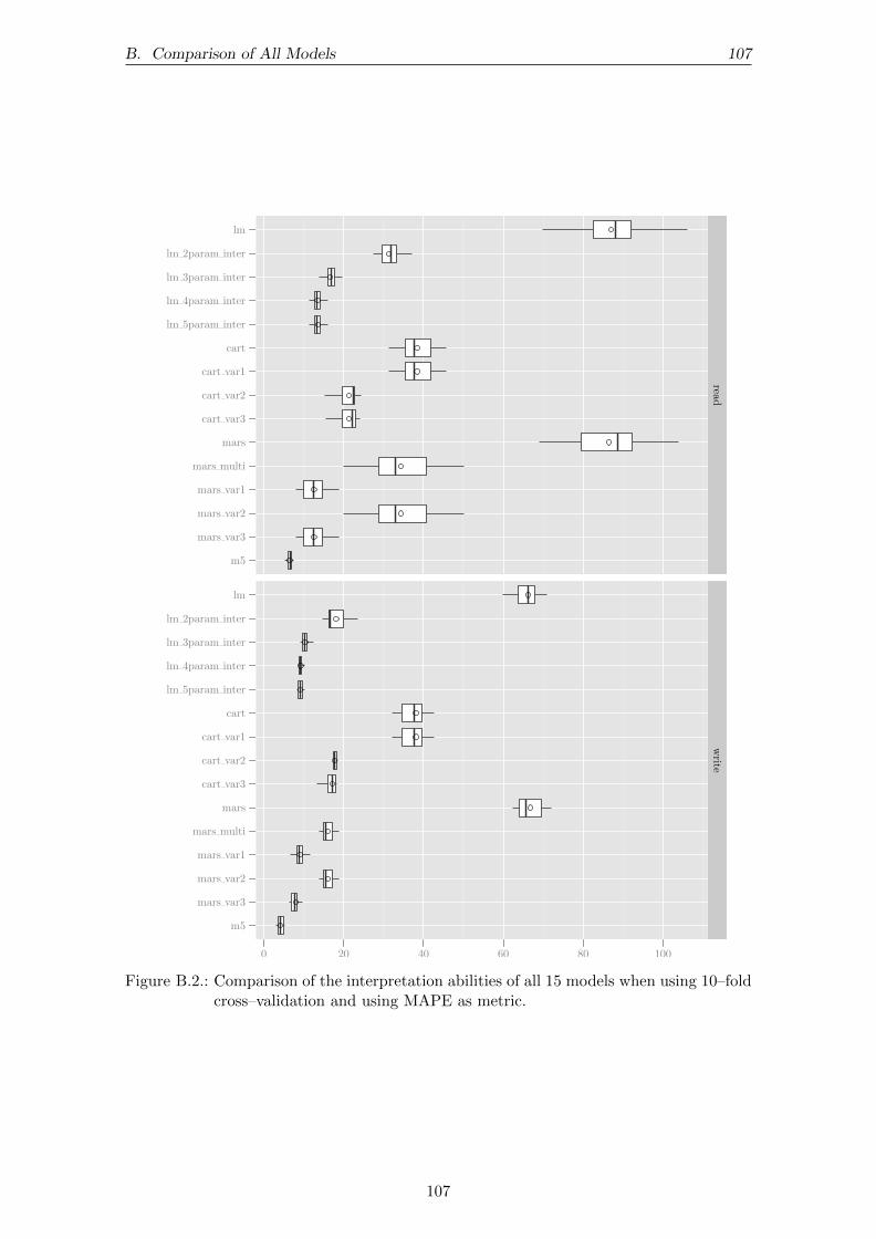
B. Comparison of All Models 107

m5

mars var3

mars var2

mars var1

mars multi

mars

cart var3

cart var2

cart var1

cart

lm 5param inter

lm 4param inter

lm 3param inter

lm 2param inter

lm

m5

mars var3

mars var2

mars var1

mars multi

mars

cart var3

cart var2

cart var1

cart

lm 5param inter

lm 4param inter

lm 3param inter

lm 2param inter

lm

read

write

0 20 40 60 80 100

Figure B.2.: Comparison of the interpretation abilities of all 15 models when using 10–foldcross–validation and using MAPE as metric.

107

108 Appendix


(ms) (%) (ms) (%)

lm 11.51 87.02 8.77 66.32lm 2param inter 4.80 31.40 3.26 18.12lm 3param inter 3.13 16.72 2.62 10.35lm 4param inter 2.95 13.43 2.56 9.26lm 5param inter 2.96 13.47 2.56 9.19cart 6.16 38.40 5.20 38.11cart var1 6.16 38.40 5.20 38.11cart var2 3.79 21.25 2.78 17.68cart var3 3.78 21.26 2.57 17.13mars 11.54 86.36 8.75 66.84mars multi 4.86 34.34 2.86 16.00mars var1 2.20 12.59 1.53 9.00mars var2 4.86 34.34 2.86 16.00mars var3 2.19 12.58 1.45 8.05m5 1.69 6.49 0.81 4.24

Table B.3.: Comparison of the interpolation and generalization abilities of all 15 models,benchmarked using 10–fold cross–validation.

Modeling PredictionModel Read Write Read Write

(s) (s) (s) (s)

lm 0.00500 0.00500 0.00167 0.00115lm 2param inter 0.00800 0.00800 0.00135 0.00135lm 3param inter 0.01200 0.01200 0.00167 0.00156lm 4param inter 0.01400 0.01500 0.00188 0.00167lm 5param inter 0.01500 0.01400 0.00177 0.00177cart 0.02500 0.02500 0.00115 0.00104cart var1 0.02500 0.02500 0.00115 0.00104cart var2 0.02600 0.02600 0.00125 0.00125cart var3 0.02700 0.02600 0.00125 0.00115mars 0.04400 0.04400 0.02083 0.02042mars multi 0.05800 0.05600 0.02125 0.02146mars var1 0.11100 0.10500 0.02542 0.02385mars var2 0.05700 0.05500 0.02198 0.02177mars var3 0.11100 0.10600 0.02521 0.02396m5 0.14600 0.18100 0.05052 0.05156

Table B.4.: Comparison of the time needed for the model creation (”Modeling”) and forthe prediction of 1000 samples (”Prediction”). The time needed for both, theread and the write models are depicted for each of the 15 models.

108

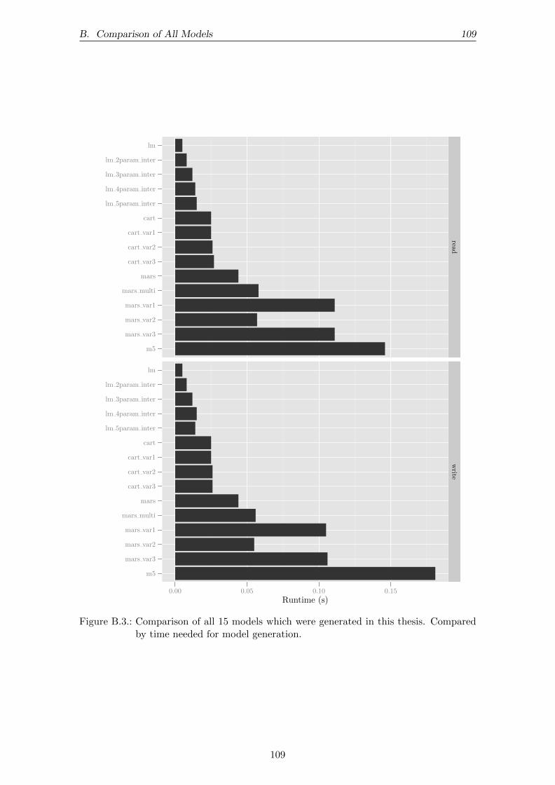
B. Comparison of All Models 109

m5

mars var3

mars var2

mars var1

mars multi

mars

cart var3

cart var2

cart var1

cart

lm 5param inter

lm 4param inter

lm 3param inter

lm 2param inter

lm

m5

mars var3

mars var2

mars var1

mars multi

mars

cart var3

cart var2

cart var1

cart

lm 5param inter

lm 4param inter

lm 3param inter

lm 2param inter

lm

read

write

0.00 0.05 0.10 0.15

Runtime (s)

Figure B.3.: Comparison of all 15 models which were generated in this thesis. Comparedby time needed for model generation.

109

110 Appendix

m5

mars var3

mars var2

mars var1

mars multi

mars

cart var3

cart var2

cart var1

cart

lm 5param inter

lm 4param inter

lm 3param inter

lm 2param inter

lm

m5

mars var3

mars var2

mars var1

mars multi

mars

cart var3

cart var2

cart var1

cart

lm 5param inter

lm 4param inter

lm 3param inter

lm 2param inter

lm

read

write

0.00 0.01 0.02 0.03 0.04 0.05

Runtime (s)

Figure B.4.: Comparison of all 15 models which were generated in this thesis. Comparedby time needed for prediction of 1000 samples.

110

C. M5 Model 111

C. M5 Model

The following two texts are a textual representation of the M5 models which were createdin this thesis. As explained, the model is so large that a graphical representation was notpossible anymore:

C.1. Read Model

Rule 1: [60 cases, mean 4.071682, range 2.186175 to 5.945354, est err 0.208076]

if

schedulerNOOP > 0

blockSize <= 16384

readPercentage > 50

sequentialAccess > 0

then

outcome = 2.249239 + 0.00023 blockSize - 0.007 readPercentage


if

schedulerNOOP > 0

blockSize <= 16384

readPercentage <= 50


then



if

filesetSize <= 25600

readPercentage > 60

sequentialAccess <= 0

then

outcome = 2.237216 + 0.00018 blockSize + 1.7e-05 filesetSize


if

schedulerNOOP > 0


readPercentage > 60


then


- 0.012 readPercentage


if

schedulerNOOP > 0

blockSize > 16384

readPercentage > 50


then



if

schedulerNOOP > 0

filesetSize <= 1024


then

outcome = 10.177727 - 0.221 readPercentage + 0.00038 blockSize


if


blockSize <= 16384



then

outcome = 12.25084 + 0.00028 filesetSize - 0.205 readPercentage

+ 0.00023 blockSize


if

schedulerNOOP > 0

filesetSize > 1024

blockSize > 16384



then


+ 1.1e-05 filesetSize


if

schedulerNOOP > 0


111

112 Appendix



then


+ 0.00026 blockSize - 1.1 schedulerNOOP + 0.5 sequentialAccess


if


blockSize > 16384



then

outcome = 16.076314 - 0.228 readPercentage + 7e-05 filesetSize

+ 0.00018 blockSize


if

schedulerNOOP <= 0

filesetSize > 25600

readPercentage > 60


then


+ 1.5 sequentialAccess + 3e-05 blockSize


if

schedulerNOOP > 0

filesetSize > 25600

readPercentage > 50


then


+ 0.0001 blockSize


if

schedulerNOOP <= 0

filesetSize > 25600

readPercentage > 40



then


- 0.00011 blockSize


if

schedulerNOOP <= 0

filesetSize <= 1024

blockSize <= 16384

readPercentage > 50


then



if

schedulerNOOP <= 0

filesetSize > 1024


blockSize <= 16384

readPercentage > 50


then



if

schedulerNOOP > 0

filesetSize > 25600



then

outcome = 30.264563 - 0.574 readPercentage + 0.000267 filesetSize

+ 0.0001 blockSize


if

schedulerNOOP <= 0

filesetSize > 25600

blockSize > 16384



then



if

schedulerNOOP <= 0

112

C. M5 Model 113

filesetSize > 1024


blockSize <= 16384



then



if

schedulerNOOP <= 0

filesetSize > 25600

blockSize <= 16384

readPercentage > 50


then

outcome = 19.700927 + 0.00153 blockSize + 3e-05 filesetSize



if

schedulerNOOP <= 0

filesetSize > 25600

blockSize <= 16384



then



if

schedulerNOOP <= 0

filesetSize > 25600

blockSize <= 16384



then


+ 0.5 sequentialAccess


if

schedulerNOOP <= 0


blockSize > 16384

readPercentage > 40


then

outcome = 31.667796 + 0.000466 filesetSize + 0.00068 blockSize



if

schedulerNOOP <= 0

filesetSize <= 1024



then



if

schedulerNOOP <= 0


blockSize > 16384



then



if

schedulerNOOP <= 0

filesetSize > 25600


blockSize > 16384

readPercentage > 40


then




if

schedulerNOOP <= 0

filesetSize > 76800

blockSize > 16384


then



113

114 Appendix

if

schedulerNOOP <= 0

filesetSize > 25600

blockSize > 16384



then


C.2. Write Model


if

filesetSize <= 1024

blockSize <= 12288


then

outcome = 3.211877 + 0.00036 blockSize + 2.8 sequentialAccess

- 0.039 readPercentage + 1.4e-05 filesetSize


if

schedulerNOOP > 0

filesetSize <= 1024

blockSize <= 20480

readPercentage > 25


then


- 0.6 schedulerNOOP + 0.4 sequentialAccess


if

schedulerNOOP > 0

filesetSize <= 1024

blockSize <= 20480

readPercentage > 0


then


- 0.5 sequentialAccess + 6e-06 filesetSize


if

schedulerNOOP > 0

filesetSize > 1024

blockSize <= 20480

readPercentage > 25


then



if

schedulerNOOP <= 0

filesetSize <= 1024

readPercentage > 25


then



if

schedulerNOOP > 0

filesetSize > 1024


readPercentage > 25


then

outcome = 11.029722 - 0.145 readPercentage + 9.5e-05 filesetSize

+ 0.00014 blockSize


if

schedulerNOOP > 0

readPercentage > 0



then

outcome = 2.116236 + 0.00041 blockSize


if

schedulerNOOP > 0

filesetSize <= 1024

blockSize > 20480

readPercentage > 0

then

114

C. M5 Model 115



if

schedulerNOOP > 0


blockSize <= 20480

readPercentage > 0



then



if

schedulerNOOP > 0

filesetSize > 51200

blockSize > 20480

readPercentage > 0


then



if

schedulerNOOP > 0

filesetSize > 1024


blockSize > 20480

readPercentage > 0


then


- 1e-05 filesetSize


if

schedulerNOOP > 0

readPercentage <= 0


then

outcome = 2.085253 + 0.00052 blockSize


if

schedulerNOOP > 0

filesetSize > 1024


blockSize > 20480

readPercentage > 0


then


+ 3.5e-05 filesetSize


if

schedulerNOOP <= 0

filesetSize > 1024

blockSize <= 4096

readPercentage > 0


then



if

schedulerNOOP <= 0

filesetSize > 1024


blockSize > 4096

readPercentage > 0


then

outcome = 9.394175 - 0.111 readPercentage + 7.3e-05 filesetSize

+ 0.00025 blockSize


if

filesetSize <= 1024

blockSize > 12288



then



if

schedulerNOOP <= 0

filesetSize > 1024


115

116 Appendix

blockSize > 16384

readPercentage > 0



then



if

schedulerNOOP > 0

filesetSize > 51200

blockSize <= 20480

readPercentage > 0


then


+ 0.00013 blockSize


if

schedulerNOOP <= 0

filesetSize > 51200

blockSize > 4096

blockSize <= 16384

readPercentage > 0


then


- 0.025 readPercentage + 0.4 sequentialAccess


if

schedulerNOOP > 0


readPercentage <= 0


then



if

schedulerNOOP > 0

filesetSize > 51200

blockSize > 20480

readPercentage > 0


then


+ 0.00015 blockSize


if

schedulerNOOP <= 0

filesetSize > 1024

blockSize > 16384

readPercentage > 60


then

outcome = -0.776021 + 0.000225 filesetSize + 0.00017 blockSize


if

schedulerNOOP <= 0

filesetSize > 25600

blockSize > 16384

readPercentage > 0



then


+ 0.044 readPercentage


if

schedulerNOOP <= 0

filesetSize > 25600

blockSize > 16384

readPercentage > 50



then



if

schedulerNOOP > 0

filesetSize > 25600

blockSize <= 20480

readPercentage <= 0


then


116

C. M5 Model 117


if

schedulerNOOP <= 0

filesetSize <= 1024

blockSize <= 16384


then



if

schedulerNOOP <= 0

filesetSize > 1024

blockSize <= 12288

readPercentage <= 0


then

outcome = 13.737529 + 0.000165 filesetSize


if

schedulerNOOP > 0

filesetSize > 25600

blockSize > 20480

readPercentage <= 0


then



if

schedulerNOOP <= 0

filesetSize > 1024

blockSize > 12288

readPercentage <= 0


then

outcome = 18.901978 + 5.7e-05 filesetSize + 0.00015 blockSize


if

schedulerNOOP <= 0

filesetSize > 1024

blockSize <= 16384


then




if

schedulerNOOP <= 0

filesetSize <= 1024

blockSize > 16384


then



if

schedulerNOOP <= 0

filesetSize > 1024

readPercentage > 60


then



if

schedulerNOOP <= 0

filesetSize > 1024


blockSize > 16384



then



if

schedulerNOOP <= 0

filesetSize > 51200

blockSize > 16384


then



117

118 Glossary

D. Glossary

benchmark is a piece of software which runs on the system under test. It produces loadon the system and captures results of given metrics. 118

benchmark controller uses the benchmark drivers to coordinate the execution of bench-marks on the systems under test. 39, 118

benchmark driver is the interface between the benchmark controller and the benchmark.It launches a given benchmark, captures the output and extracts the results fromthe output. 39, 41, 118

benchmark harness consists of multiple components which help to plan and control theexecution of benchmarks on multiple hosts, gather the results and store them forfurther analysis. 118

benchmark run A single execution of a benchmark on one system under test. 118

dependent variable is a variable, whose values are generated during the run of a bench-mark. The values are dependent on the values of the independent variables. 5, 24,118

experiment is a specification of one benchmark run defined by a value for each of theindependent variables needed and a system under test where the benchmark runshould be executed on. 41, 118

experiment series is a term used in singular form for a set of experiments on a systemunder test. The experiments are defined by a independent variable space. 42, 118

experiment setup defines the overall experiment configuration. It contains an experimentseries for each system under test which will be involved. 118

independent variable is also called an explanatory variable or input variable. It is avariable whose values are set prior to the run of a benchmark. It includes all factorswhich can possibly change the outcome of a benchmark. 5, 6, 24, 41, 118

independent variable space is a set of independent variables and one or more values foreach of the variables. 42, 118

system under test is the actual host or machine for which the benchmark results shouldbe generated. 41, 118

118

List of Figures

3.1. Architecture of the IBM DS8700. . . . . . . . . . . . . . . . . . . . . . . . . 10

3.2. Options to run Linux on IBM System z. . . . . . . . . . . . . . . . . . . . . 11

3.3. Possible performance influencing factors (based on [NKR12]). . . . . . . . . 13

3.4. Different layers a requests issued by the FFSB Benchmark has to go through.Layers marked with a thunderbolt contain caches which can speed up re-sponses but also make predictions more difficult. . . . . . . . . . . . . . . . 16

4.1. Example boxplot including labels as explanation. . . . . . . . . . . . . . . . 20

4.2. Example cumulative distribution function using the same data as the box-plot in Figure 4.1. . . . . . . . . . . . . . . . . . . . . . . . . . . . . . . . . 21

4.3. Example linear regression (straight line) of a sample set containing oneinput variable x and output variable y (printed as dots). . . . . . . . . . . . 26

4.4. MARS basis function pair for t = 0.5. . . . . . . . . . . . . . . . . . . . . . 27

4.5. Comparison between a linear regression model and a MARS model fittedto the same data. The regressions are shown as straight lines, the sampleset is printed as dots. . . . . . . . . . . . . . . . . . . . . . . . . . . . . . . . 28

4.6. Example for a regression tree containing two input variables (”area” and”peri”) and an output variable. . . . . . . . . . . . . . . . . . . . . . . . . . 29

4.7. Regression tree before pruning: This figure shows the output of the first stepwhich will be pruned in the second step of the regression tree generation.Compare to Figure 4.6 which shows the same tree after the pruning step. . 30

4.8. Example M5 model consisting of the regression tree and the attached linearmodels. The left edge of a node in the regression tree must be evaluated ifthe condition is true, the right edge if the condition is false. . . . . . . . . . 32

4.9. Example for an overfitted model on the left and a non overfitted modelusing the same samples on the right. . . . . . . . . . . . . . . . . . . . . . . 34

4.10. Steps necessary for k–fold cross–validation. . . . . . . . . . . . . . . . . . . 36

5.1. Overview of the components involved. Dashed components are existing andtherefore reused. Two additional benchmark have been included in thediagram for demonstration purposes. Currently only an FFSB benchmarkdriver is available. Other benchmark drivers can nevertheless be added easily. 40

5.2. Class diagram for the benchmark drivers and the other classes involved inthis context. . . . . . . . . . . . . . . . . . . . . . . . . . . . . . . . . . . . . 41

5.3. Class diagram for the classes used to represent the configuration for thebenchmarking process. . . . . . . . . . . . . . . . . . . . . . . . . . . . . . . 42

5.4. Object diagram of a configuration instance. . . . . . . . . . . . . . . . . . . 43

5.5. Class diagram for the runnable parts of the harness which includes thecontroller and the data store. . . . . . . . . . . . . . . . . . . . . . . . . . . 44

5.6. GQM plan schema (based on [BCR94] and [Fab11]). . . . . . . . . . . . . . 46

119

120 List of Figures

6.1. Top 5 experiments with the highest standard deviation in the mean responsetime of their repeats. . . . . . . . . . . . . . . . . . . . . . . . . . . . . . . . 50

6.2. Boxplot and cumulative distribution function visualizing the distribution ofthe relative error in the repetition of the experiments. . . . . . . . . . . . . 51

6.3. Pie chart of the amount of influence on the variation of the response timeper parameter. Missing values to 100% are the influence of the residuals. . . 53

6.4. Pie chart of the amount of influence on the variation of the response timeper parameter. It includes interactions between two parameters. Valuessmaller than 5% have been aggregated to ”other”. Missing values to 100%are the influence of the residuals. . . . . . . . . . . . . . . . . . . . . . . . . 54

6.5. Boxplots and CDF for the relative errors of the read and the write requests.The relative error between the case when running the benchmark on twoseparate virtual machines and the case when running a single benchmarkon a single virtual machine is depicted here. . . . . . . . . . . . . . . . . . . 58

6.6. Boxplots comparing the relative errors depending on the read percentage.The read percentage is the amount of operations which are read requests. . 59

7.1. Comparison of the quality of models generated using the full data set. Twodifferent metrics were used: Root Mean Square Error (RMSE) and MediumAbsolute Percentage error (MAPE). . . . . . . . . . . . . . . . . . . . . . . 64

7.2. Comparison of the interpolation abilities of the nine regression models testedusing 200 newly collected randomly selected samples. . . . . . . . . . . . . . 67

7.3. Extrapolation abilities of the regression models, trained using a reduceddata set and tested using the left out samples. . . . . . . . . . . . . . . . . . 69

7.4. Extrapolation abilities of all models, tested using randomly newly bench-marked data. . . . . . . . . . . . . . . . . . . . . . . . . . . . . . . . . . . . 72

7.5. Extrapolation abilities for read requests of the linear model including allinteractions (lm 5param inter) and the M5 model (m5). The test data wassplit into two sets: a ”low” set containing the block sizes ≤ 2 kB and the”high” set containing the block sizes ≥ 36 kB. The metric depicted is RMSE. 73

7.6. Comparison of the quality of the nine regression models built using thereduced data set red1. The models were tested using 200 randomly drawnsamples from the complete sample set. . . . . . . . . . . . . . . . . . . . . . 75

7.7. Comparison of the quality of the nine regression models built using thereduced data set red2. The metrics were calculated using 200 randomlydrawn samples from the whole 1120 sample set. . . . . . . . . . . . . . . . . 76

7.8. Computed MAPE and RMSE values if separated models are built for eachvalue of nominal scale parameters. This means that four models were cre-ated and the average of the RMSE and MAPE is depicted here. . . . . . . . 78

7.9. The split models, where four different models are used, compared to theoriginal models using a single model. A negative value means an improve-ment due to the splitting, a positive value means decline due to the splitting. 79

7.10. Comparison of the time needed for the generation of a single model of eachof the regression techniques. . . . . . . . . . . . . . . . . . . . . . . . . . . . 84

7.11. Comparison of the time needed for the prediction of 1000 samples for eachof the regression techniques. . . . . . . . . . . . . . . . . . . . . . . . . . . . 85

7.12. CART model for the whole data set. . . . . . . . . . . . . . . . . . . . . . . 87

7.13. M5 Model: The model depicted here is not the actual model which wascreated in the thesis. The real model has more than four times the size ofthis smaller model which does not show all branches of the original model.This model is depicted to show how interpretable the results are. . . . . . 91

120

List of Figures 121

7.14. Comparison of the quality of model constructed using different values forthe configuration parameters of the MARS algorithm. . . . . . . . . . . . . 94

7.15. Comparison of the four different configurations for the CART algorithm.The unmodified CART model and the best linear regression model are in-cluded for comparison reasons. . . . . . . . . . . . . . . . . . . . . . . . . . 96

B.1. Comparison of all 15 models which were generated in this thesis using RMSEwhen using 10–fold cross–validation to test the interpretation abilities. . . . 106

B.2. Comparison of the interpretation abilities of all 15 models when using 10–fold cross–validation and using MAPE as metric. . . . . . . . . . . . . . . . 107

B.3. Comparison of all 15 models which were generated in this thesis. Comparedby time needed for model generation. . . . . . . . . . . . . . . . . . . . . . . 109

B.4. Comparison of all 15 models which were generated in this thesis. Comparedby time needed for prediction of 1000 samples. . . . . . . . . . . . . . . . . 110

121

List of Tables

4.1. Sample table for the organization of the input to the ANOVA analysis(source: [Kou11]). . . . . . . . . . . . . . . . . . . . . . . . . . . . . . . . . 22

4.2. Example ANOVA result for an analysis of two parameters with interactions(based on [Kou11]). . . . . . . . . . . . . . . . . . . . . . . . . . . . . . . . . 24

5.1. Values of the parameters which are varied in this thesis. These values leadto a total of 1120 configurations when using full exploration. . . . . . . . . 39

5.2. Examples for independent variable spaces. . . . . . . . . . . . . . . . . . . . 42

5.3. Example for the full exploration of an experiment series containing thevariable spaces defined above in Table 5.2. . . . . . . . . . . . . . . . . . . . 43

5.4. The GQM plan for this thesis with references to the matching sections inthe following chapters. . . . . . . . . . . . . . . . . . . . . . . . . . . . . . . 47

6.1. The underlying statistical values for the boxplot in Figure 6.2. . . . . . . . 51

6.2. Multidimensional ANOVA test on all parameters without interactions. . . . 53

6.3. Multidimensional ANOVA test on all parameters including interaction termsbetween two parameters. . . . . . . . . . . . . . . . . . . . . . . . . . . . . . 54

6.4. Multidimensional ANOVA test on all parameters including interactions be-tween two parameters. Only two values were included for each parameter,leading to a n2m ANOVA and a reduction of the required benchmark runs. 56

6.5. Underlying data for the boxplot in Figure 6.5. . . . . . . . . . . . . . . . . . 57

7.1. Underlying data for the boxplots in Figure 7.1, which show the comparisonof the interpolation abilities of the regression models when tested using10-fold cross–validation. . . . . . . . . . . . . . . . . . . . . . . . . . . . . . 63

7.2. Comparison of the interpolation abilities when using 200 newly collectedrandom samples. This is the underlying data for the bar plots in Figure 7.2. 66

7.3. Comparison of the extrapolation abilities when reducing the original sampleset by removing the extreme values and reuse the removed samples fortraining. This is the underlying data for the bar plots in Figure 7.3. . . . . 68

7.4. Comparison of the extrapolation abilities when using the original modelsand testing using random newly benchmarked data. This data is depictedas bar plots in Figure 7.4. . . . . . . . . . . . . . . . . . . . . . . . . . . . . 71

7.5. Two reduced samples sets which are used to test if accurate models can begenerated using a smaller number of samples. . . . . . . . . . . . . . . . . . 74

7.6. Generalizationa abilities of regression models which were built separate forthe values of the nominal scales. Figure 7.8 contains a graphical represen-tation. . . . . . . . . . . . . . . . . . . . . . . . . . . . . . . . . . . . . . . . 78

7.7. Comparison of the different experiments conducted in the previous sections. 81

7.8. Comparison of the time needed for the model creation (”Modeling”) and forthe prediction of 1000 samples (”Prediction”). The time needed for both,the read and the write models is depicted. . . . . . . . . . . . . . . . . . . . 84

123

124 List of Tables

7.9. Linear regression model without interactions. The table shows the values forthe coefficients for both, the read and the write model. All values roundedto five digits. . . . . . . . . . . . . . . . . . . . . . . . . . . . . . . . . . . . 86

7.10. Linear regression model with all interaction terms, including those betweentwo, three, four, and five parameters. The coefficients for both, the readand write model, are shown in the columns. All values are rounded to fivedigits. . . . . . . . . . . . . . . . . . . . . . . . . . . . . . . . . . . . . . . . 88

7.11. MARS model. . . . . . . . . . . . . . . . . . . . . . . . . . . . . . . . . . . . 897.12. Multidimensional MARS model. . . . . . . . . . . . . . . . . . . . . . . . . 907.13. Strengths and weaknesses of the different regression techniques and models.

The comparison is done using a relative rating of one to four stars. Therating does only provide a relative ranking and does not account otherexisting modeling techniques. The ”Simplicity of Algorithm” should beseen as the opposite of the complexity of the algorithm. . . . . . . . . . . . 92

7.14. Different values for the MARS regression technique configuration parame-ters. The first column shows the name of the configuration. . . . . . . . . . 93

7.15. Different values for the CART regression technique configuration parame-ters. The first column shows the name of the configuration. . . . . . . . . . 95

A.1. ANOVA containing all interactions for read requests. . . . . . . . . . . . . . 104A.2. ANOVA for write response times containing all interactions. . . . . . . . . . 105B.3. Comparison of the interpolation and generalization abilities of all 15 models,

benchmarked using 10–fold cross–validation. . . . . . . . . . . . . . . . . . . 108B.4. Comparison of the time needed for the model creation (”Modeling”) and for

the prediction of 1000 samples (”Prediction”). The time needed for both,the read and the write models are depicted for each of the 15 models. . . . 108

124

Bibliography

[AAH+03] I. Ahmad, J. Anderson, A. Holler, R. Kambo, and V. Makhija, “An analysisof disk performance in VMware ESX Server virtual machines,” in Work-load Characterization, 2003. WWC-6. 2003 IEEE International Workshopon. IEEE, 2003, pp. 65–76.

[And01] E. Anderson, “Simple table-based modeling of storage devices,” HP Labora-tories, SSP technical report, July 2001.

[BCR94] V. R. Basili, G. Caldiera, and H. D. Rombach, “The goal question metricapproach,” Encyclopedia of Software Engineering, pp. 528–532, 1994.

[BFS+06] F. Benevenuto, C. Fernandes, M. Santos, V. Almeida, J. Almeida, G. Janaki-raman, and J. Santos, “Performance models for virtualized applications,”in Frontiers of High Performance Computing and Networking – ISPA 2006Workshops, ser. Lecture Notes in Computer Science, G. Min, B. Di Martino,L. Yang, M. Guo, and G. Runger, Eds. Springer Berlin / Heidelberg, 2006,vol. 4331, pp. 427–439.

[BFSO84] L. Breiman, J. Friedman, C. J. Stone, and R. Olshen, Classification andregression trees, ser. The Wadsworth and Brooks-Cole statistics-probabilityseries. Chapman & Hall, 1984.

[BKR09] S. Becker, H. Koziolek, and R. Reussner, “The palladio component modelfor model-driven performance prediction,” J. Syst. Softw., vol. 82, no. 1, pp.3–22, Jan. 2009.

[CHC+01] Y. M. Chae, S. H. Ho, K. W. Cho, D. H. Lee, and S. H. Ji, “Data min-ing approach to policy analysis in a health insurance domain,” InternationalJournal of Medical Informatics, vol. 62, Issue 2, pp. 103–111, 2001.

[CKK11] G. Casale, S. Kraft, and D. Krishnamurthy, “A model of storage I/O perfor-mance interference in virtualized systems,” in 31st IEEE International Con-ference on Distributed Computing Systems Workshops (ICDCS 2011 Work-shops), 20-24 June 2011, Minneapolis, Minnesota, USA. IEEE ComputerSociety, 2011, pp. 34–39.

[CW00] M. Courtois and M. Woodside, “Using regression splines for software perfor-mance analysis,” in Proceedings of the 2nd international workshop on Soft-ware and performance, ser. WOSP ’00. New York, NY, USA: ACM, 2000,pp. 105–114.

[DBC+10] B. Dufrasne, W. Bauer, B. Careaga, J. Myyrrylainen, A. Rainero, andP. Usong, IBM System Storage DS8700: Architecture and Implementation.IBM Corporation, International Technical Support Organization, 2010.

[DSW03] B. Dufrasne, D. Skilton, and J. Wright, Linux with zSeries and ESS: Es-sentials. IBM Corporation, International Technical Support Organization,2003.

125

126 Bibliography

[Fab] Faban, “Harness and benchmark framework,” last visited 2012/07/22.[Online]. Available: http://java.net/projects/faban/

[Fab11] M. Faber, “Software performance analysis using machine learning tech-niques,” Master’s thesis, Institute for Program Structures and Data Orga-nization (IPD), Karlsruhe Institute of Technology, March 2011.

[Fri91] J. H. Friedman, “Multivariate adaptive regression splines.” Ann. Stat.,vol. 19, no. 1, pp. 1–141, 1991.

[HBR+10] N. Huber, S. Becker, C. Rathfelder, J. Schweflinghaus, and R. H. Reussner,“Performance modeling in industry: A case study on storage virtualization,”in Proceedings of the 32nd ACM/IEEE International Conference on SoftwareEngineering - Volume 2, ser. ICSE ’10. New York, NY, USA: ACM, 2010,pp. 1–10.

[HEK05] J. Hartung, B. Elpelt, and K.-H. Klosener, Statistik: Lehr- und Handbuch derangewandten Statistik, 14th ed. Munchen: Oldenbourg Wissenschaftsverlag,2005.

[HKHR11] M. Hauck, M. Kuperberg, N. Huber, and R. Reussner, “Ginpex: Derivingperformance-relevant infrastructure properties through goal-oriented experi-ments,” in Proceedings of the joint ACM SIGSOFT conference – QoSA andACM SIGSOFT symposium – ISARCS on Quality of software architectures– QoSA and architecting critical systems – ISARCS, ser. QoSA-ISARCS ’11.New York, NY, USA: ACM, 2011, pp. 53–62.

[HTF11] T. Hastie, R. Tibshirani, and J. Friedman, The Elements of Statistical Learn-ing: Data Mining, Inference, and Prediction, Second Edition, ser. SpringerSeries in Statistics. Springer, 2011.

[HvQHK11] N. Huber, M. von Quast, M. Hauck, and S. Kounev, “Evaluating and mod-eling virtualization performance overhead for cloud environments,” in 1st In-ternational Conference on Cloud Computing and Services Science (CLOSER2011), May, 2011, pp. 7–9.

[KCK+11] S. Kraft, G. Casale, D. Krishnamurthy, D. Greer, and P. Kilpatrick, “IO per-formance prediction in consolidated virtualized environments,” in Proceedingsof the second joint WOSP/SIPEW international conference on Performanceengineering, ser. ICPE ’11. New York, NY, USA: ACM, 2011, pp. 295–306.

[KCK+12] ——, “Performance models of storage contention in cloud environments,”Springer Journal of Software and Systems Modeling, pp. 1–24, 2012.

[KKB+07] Y. Koh, R. Knauerhase, P. Brett, M. Bowman, Z. Wen, and C. Pu, “Ananalysis of performance interference effects in virtual environments,” in Per-formance Analysis of Systems & Software, 2007. ISPASS 2007. IEEE Inter-national Symposium on. IEEE, 2007, pp. 200–209.

[KLSC07] H. Kim, W.-y. Loh, Y.-s. Shih, and P. Chaudhuri, “Visualizable and inter-pretable regression models with good prediction power,” IIE Transactions,vol. 39, p. 565–579, 2007.

[Kou11] S. Kounev, “Performance engineering of enterprise software systems,”2011, University Lecture, last visited 2012/06/26. [Online]. Avail-able: http://sdqweb.ipd.kit.edu/wiki/Vorlesung Performance Engineeringof Enterprise Software Systems SS2011

126

http://java.net/projects/faban/

http://sdqweb.ipd.kit.edu/wiki/Vorlesung_Performance_Engineering_of_Enterprise_Software_Systems_SS2011

http://sdqweb.ipd.kit.edu/wiki/Vorlesung_Performance_Engineering_of_Enterprise_Software_Systems_SS2011

Bibliography 127

[KRDZ10] S. Kundu, R. Rangaswami, K. Dutta, and M. Zhao, “Application performancemodeling in a virtualized environment,” in High Performance Computer Ar-chitecture (HPCA), 2010 IEEE 16th International Symposium on. IEEE,2010, pp. 1–10.

[Kuh08] M. Kuhn, “Building predictive models in R using the caret package,”Journal of Statistical Software, vol. 28, no. 5, pp. 1–26, 11 2008. [Online].Available: http://www.jstatsoft.org/v28/i05

[Kva85] T. O. Kvalseth, “Cautionary note about R2,” The American Statistician,vol. 39, no. 4, pp. 279–285, Nov. 1985.

[LK93] E. K. Lee and R. H. Katz, “An analytic performance model of disk arrays,”SIGMETRICS Perform. Eval. Rev., vol. 21, no. 1, pp. 98–109, Jun. 1993.

[MCCS08] N. Mi, G. Casale, L. Cherkasova, and E. Smirni, “Burstiness in multi-tierapplications: Symptoms, causes, and new models,” in Proceedings of the 9thACM/IFIP/USENIX International Conference on Middleware, ser. Middle-ware ’08. New York, NY, USA: Springer-Verlag New York, Inc., 2008, pp.265–286.

[Mei08] S. Meier, IBM Systems Virtualization: Servers, Storage, and Software. IBMCorporation, International Technical Support Organization, 2008.

[MF02] G. Moisen and T. Frescino, “Comparing five modelling techniques for predict-ing forest characteristics,” Ecological Modelling, vol. 157, no. 2, pp. 209–225,2002.

[NKR12] Q. Noorshams, S. Kounev, and R. Reussner, “Experimental evaluation of theperformance-influencing factors of virtualized storage systems,” in Proceed-ings of the 9th European Performance Engineering Workshop (EPEW’12),Munich, Germany, July 30-31, 2012.

[PBH+08] L. Parziale, M. Belardi, M. Held, L. Y. Ma, L. Peckover, and K. Reed, Linuxon IBM System z: Performance Measurement and Tuning. IBM Corpora-tion, International Technical Support Organization, 2008.

[Qui92] J. Quinlan, “Learning with continuous classes,” in Proceedings of the 5thAustralian joint Conference on Artificial Intelligence. Singapore, 1992, pp.343–348.

[Ste07] P. Sterlin, “Overfitting prevention with cross-validation,” Master’s thesis,Laboratoire d’Informatique de Paris 6 (LIP6), 2007.

[TKKO05] M. Ture, I. Kurt, A. T. Kurum, and K. Ozdamar, “Comparing classifica-tion techniques for predicting essential hypertension,” Expert Systems withApplications, vol. 29, no. 3, pp. 583–588, 2005.

[vBK04] W. C. M. van Beers and J. P. C. Kleijnen, “Kriging interpolation in simula-tion: A survey,” in Proceedings of the 36th conference on Winter simulation,ser. WSC ’04. Winter Simulation Conference, 2004, pp. 113–121.

[WAA+04] M. Wang, K. Au, A. Ailamaki, A. Brockwell, C. Faloutsos, and G. R. Ganger,“Storage device performance prediction with CART models,” in Proceedingsof the The IEEE Computer Society’s 12th Annual International Symposiumon Modeling, Analysis, and Simulation of Computer and TelecommunicationsSystems. Washington, DC, USA: IEEE Computer Society, 2004, pp. 588–595.

127

http://www.jstatsoft.org/v28/i05

128 Bibliography

[WH11] D. Westermann and J. Happe, “Performance cockpit: Systematic measure-ments and analyses,” in Proceedings of the second joint WOSP/SIPEW inter-national conference on Performance engineering, ser. ICPE ’11. New York,NY, USA: ACM, 2011, pp. 421–422.

[WHHH10] D. Westermann, J. Happe, M. Hauck, and C. Heupel, “The performancecockpit approach: A framework for systematic performance evaluations,” inSoftware Engineering and Advanced Applications (SEAA), 2010 36th EU-ROMICRO Conference on. IEEE, 2010, pp. 31–38.

[WHKF12] D. Westermann, J. Happe, R. Krebs, and R. Farahbod, “Automated infer-ence of goal-oriented performance prediction functions,” in 27th IEEE/ACMInternational Conference On Automated Software Engineering (ASE 2012),September 2012.

128

Modeling and Experimental Analysis of Virtualized Storage ...

Documents

Transcript of Modeling and Experimental Analysis of Virtualized Storage ...