Clemson University Clemson University

TigerPrints TigerPrints

All Dissertations Dissertations

December 2020

Modeling and Analysis of Scheduling Problems Containing Modeling and Analysis of Scheduling Problems Containing

Renewable Energy Decisions Renewable Energy Decisions

Shasha Wang Clemson University, sarahwsasa@gmail.com

Follow this and additional works at: https://tigerprints.clemson.edu/all_dissertations

Recommended Citation Recommended Citation Wang, Shasha, "Modeling and Analysis of Scheduling Problems Containing Renewable Energy Decisions" (2020). All Dissertations. 2724. https://tigerprints.clemson.edu/all_dissertations/2724

This Dissertation is brought to you for free and open access by the Dissertations at TigerPrints. It has been accepted for inclusion in All Dissertations by an authorized administrator of TigerPrints. For more information, please contact kokeefe@clemson.edu.

Modeling and Analysis of Scheduling ProblemsContaining Renewable Energy Decisions

A Dissertation

Presented to

the Graduate School of

Clemson University

In Partial Fulfillment

of the Requirements for the Degree

Doctor of Philosophy

Industrial Engineering

by

Shasha Wang

December 2020

Accepted by:

Dr. Scott J. Mason, Committee Chair

Dr. Mary E. Kurz

Dr. Harsha Gangammanavar

Dr. Yongjia Song

Abstract

With globally increasing energy demands, world citizens are facing one of so-

ciety’s most critical issues: protecting the environment. To reduce the emission of

greenhouse gases (GHG), which are by-products of conventional energy resources,

people are reducing the consumption of oil, gas, and coal collectively. In the mean-

while, interest in renewable energy resources has grown in recent years. Renewable

generators can be installed both on the power grid side and end-use customer side of

power systems. Energy management in power systems with multiple microgrids con-

taining renewable energy resources has been a focus of industry and researchers as of

late. Further, on-site renewable energy provides great opportunities for manufactur-

ing plants to reduce energy costs when faced with time-varying electricity prices. To

efficiently utilize on-site renewable energy generation, production schedules and en-

ergy supply decisions need to be coordinated. As renewable energy resources like solar

and wind energy typically fluctuate with weather variations, the inherent stochastic

nature of renewable energy resources makes the decision making of utilizing renewable

generation complex.

In this dissertation, we study a power system with one main grid (arbiter) and

multiple microgrids (agents). The microgrids (MGs) are equipped to control their

local generation and demand in the presence of uncertain renewable generation and

heterogeneous energy management settings. We propose an extension to the classical

ii

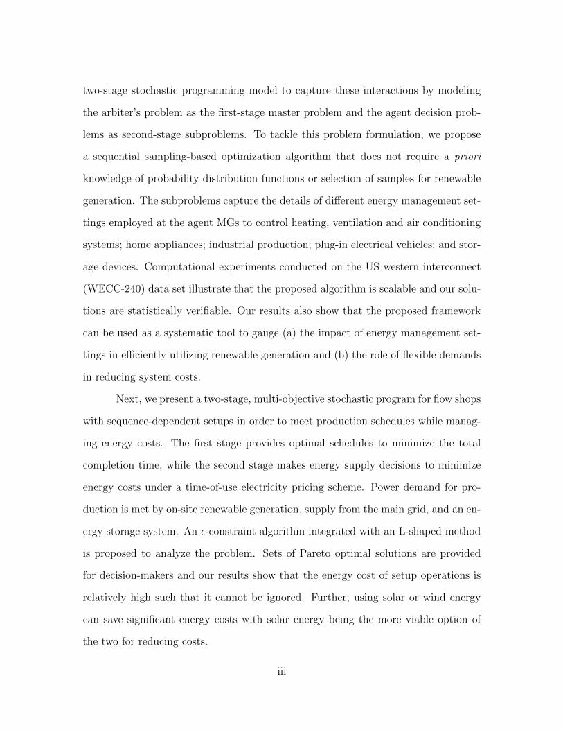
two-stage stochastic programming model to capture these interactions by modeling

the arbiter’s problem as the first-stage master problem and the agent decision prob-

lems as second-stage subproblems. To tackle this problem formulation, we propose

a sequential sampling-based optimization algorithm that does not require a priori

knowledge of probability distribution functions or selection of samples for renewable

generation. The subproblems capture the details of different energy management set-

tings employed at the agent MGs to control heating, ventilation and air conditioning

systems; home appliances; industrial production; plug-in electrical vehicles; and stor-

age devices. Computational experiments conducted on the US western interconnect

(WECC-240) data set illustrate that the proposed algorithm is scalable and our solu-

tions are statistically verifiable. Our results also show that the proposed framework

can be used as a systematic tool to gauge (a) the impact of energy management set-

tings in efficiently utilizing renewable generation and (b) the role of flexible demands

in reducing system costs.

Next, we present a two-stage, multi-objective stochastic program for flow shops

with sequence-dependent setups in order to meet production schedules while manag-

ing energy costs. The first stage provides optimal schedules to minimize the total

completion time, while the second stage makes energy supply decisions to minimize

energy costs under a time-of-use electricity pricing scheme. Power demand for pro-

duction is met by on-site renewable generation, supply from the main grid, and an en-

ergy storage system. An ε-constraint algorithm integrated with an L-shaped method

is proposed to analyze the problem. Sets of Pareto optimal solutions are provided

for decision-makers and our results show that the energy cost of setup operations is

relatively high such that it cannot be ignored. Further, using solar or wind energy

can save significant energy costs with solar energy being the more viable option of

the two for reducing costs.

iii

Finally, we extend the flow shop scheduling problem to a job shop environment

under hour-ahead real-time electricity pricing schemes. The objectives of interest are

to minimize total weighted completion time and energy costs simultaneously. Besides

renewable generation, hour-ahead real-time electricity pricing is another source of

uncertainty in this study as electricity prices are released to customers only hours

in advance of consumption. A mathematical model is presented and an ε-constraint

algorithm is used to tackle the bi-objective problem. Further, to improve computa-

tional efficiency and generate solutions in a practically acceptable amount of time, a

hybrid multi-objective evolutionary algorithm based on the Non-dominated Sorting

Genetic Algorithm II (NSGA-II) is developed. Five methods are developed to calcu-

late chromosome fitness values. Computational tests show that both mathematical

modeling and our proposed algorithm are comparable, while our algorithm produces

solutions much quicker. Using a single method (rather than five) to generate sched-

ules can further reduce computational time without significantly degrading solution

quality.

iv

Dedication

This dissertation is dedicated to my dearest son, Ethan Yifei Wang, who

showed me the happiness of being a mom; To my loving husband, Dr. Tianwei

Wang, who has always supported me; To my parents, Lijuan Zhou and Jianzhong

Wang, whom have given all of their love to me.

v

Acknowledgements

First and foremost, I would like to express my sincere gratitude to my advisor,

Dr. Scott J. Mason, for his support, guidance, and motivation throughout my Ph.D.

study. I really appreciate that he has provided me with the research freedom to

explore on my own interests and the guidance to keep me on the right path. He also

gave me the freedom to choose the location and time to do my research such that

I can take good care of my family. He is the best advisor and mentor I have ever

known.

I would also like to extend my gratitude to my committee members: Dr.

Harsha Gangammanavar, Dr. Mary E. Kurz, and Dr. Yongjia Song. Dr. Harsha

Gangammanavar was my research mentor when he was a post-doc at Clemson Univer-

sity. He taught me how to conduct research. I thank him for his patience, motivation,

enthusiasm, and immense knowledge. Profound gratitude goes to Dr. Mary E. Kurz

for her encouragement, insightful comments, and patient guidance throughout the

process of my dissertation. I am thankful to Dr. Yongjia Song for his guidance and

directions given to me for completing my dissertation. Special thanks go to Dr. San-

dra D. Eksioglu for her suggestions and comments in completing this project during

her time at Clemson.

I would like to thank my friends, Dr. Site Wang, Dr. Mowen Lu, Dr. Sreenath

Chalil Madathil, Dr. Zahra Azadi, and Di Liu for providing their help and support

vi

in my research and life.

Last but not the least, many thanks to my dear husband, Dr. Tianwei Wang,

who was always there for me and stood by me through both good times and bad. I

also profoundly thank my parents for supporting me and encouraging me with their

best wishes. Finally, thanks go to my little angel, Ethan Yifei Wang, for bringing me

happiness and perspective during the writing of this dissertation.

vii

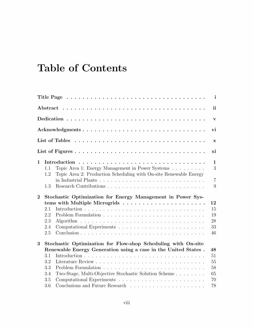
Table of Contents

Title Page . . . . . . . . . . . . . . . . . . . . . . . . . . . . . . . . . . . i

Abstract . . . . . . . . . . . . . . . . . . . . . . . . . . . . . . . . . . . . ii

Dedication . . . . . . . . . . . . . . . . . . . . . . . . . . . . . . . . . . . v

Acknowledgments . . . . . . . . . . . . . . . . . . . . . . . . . . . . . . . vi

List of Tables . . . . . . . . . . . . . . . . . . . . . . . . . . . . . . . . . x

List of Figures . . . . . . . . . . . . . . . . . . . . . . . . . . . . . . . . . xi

1 Introduction . . . . . . . . . . . . . . . . . . . . . . . . . . . . . . . . 11.1 Topic Area 1: Energy Management in Power Systems . . . . . . . . . 31.2 Topic Area 2: Production Scheduling with On-site Renewable Energy

in Industrial Plants . . . . . . . . . . . . . . . . . . . . . . . . . . . . 71.3 Research Contributions . . . . . . . . . . . . . . . . . . . . . . . . . . 9

2 Stochastic Optimization for Energy Management in Power Sys-tems with Multiple Microgrids . . . . . . . . . . . . . . . . . . . . . 122.1 Introduction . . . . . . . . . . . . . . . . . . . . . . . . . . . . . . . . 152.2 Problem Formulation . . . . . . . . . . . . . . . . . . . . . . . . . . . 192.3 Algorithm . . . . . . . . . . . . . . . . . . . . . . . . . . . . . . . . . 282.4 Computational Experiments . . . . . . . . . . . . . . . . . . . . . . . 332.5 Conclusion . . . . . . . . . . . . . . . . . . . . . . . . . . . . . . . . . 46

3 Stochastic Optimization for Flow-shop Scheduling with On-siteRenewable Energy Generation using a case in the United States . 483.1 Introduction . . . . . . . . . . . . . . . . . . . . . . . . . . . . . . . . 513.2 Literature Review . . . . . . . . . . . . . . . . . . . . . . . . . . . . . 553.3 Problem Formulation . . . . . . . . . . . . . . . . . . . . . . . . . . . 583.4 Two-Stage, Multi-Objective Stochastic Solution Scheme . . . . . . . . 653.5 Computational Experiments . . . . . . . . . . . . . . . . . . . . . . . 703.6 Conclusions and Future Research . . . . . . . . . . . . . . . . . . . . 78

viii

4 A Hybrid Multi-objective Evolutionary Algorithm for Job-shopScheduling with On-site Renewable Energy Generation and Real-time Electricity Pricing . . . . . . . . . . . . . . . . . . . . . . . . . 804.1 Introduction . . . . . . . . . . . . . . . . . . . . . . . . . . . . . . . . 824.2 Literature Review . . . . . . . . . . . . . . . . . . . . . . . . . . . . . 834.3 Model . . . . . . . . . . . . . . . . . . . . . . . . . . . . . . . . . . . 854.4 A Hybrid Multi-objective Evolutionary Algorithm . . . . . . . . . . . 904.5 Computational Experiments . . . . . . . . . . . . . . . . . . . . . . . 984.6 Conclusions and Future Research . . . . . . . . . . . . . . . . . . . . 104

5 Conclusions and Future Research . . . . . . . . . . . . . . . . . . . 1065.1 Research Conclusions . . . . . . . . . . . . . . . . . . . . . . . . . . . 1065.2 Future Research Directions . . . . . . . . . . . . . . . . . . . . . . . . 108

Bibliography . . . . . . . . . . . . . . . . . . . . . . . . . . . . . . . . . . 110

ix

List of Tables

2.1 Details of the WECC-240 power system . . . . . . . . . . . . . . . . . 352.2 Comparison between 2-SP and MA-SP . . . . . . . . . . . . . . . . . 362.3 Results of MA-SD(a) . . . . . . . . . . . . . . . . . . . . . . . . . . . 392.4 Results of MA-SD(m) . . . . . . . . . . . . . . . . . . . . . . . . . . . 402.5 Solution results of various network constraints . . . . . . . . . . . . . 422.6 Solution method comparison (Fixed and Flexible) . . . . . . . . . . . 43

3.1 Summary of reviewed ECA production scheduling problems . . . . . 593.2 Input ε, corresponding TWCT, and predicted EC of Ins3s . . . . . . 72

4.1 Experiment design . . . . . . . . . . . . . . . . . . . . . . . . . . . . 994.2 Common parameters for 30 instances . . . . . . . . . . . . . . . . . . 994.3 Mathematical Model vs. NSGA-II . . . . . . . . . . . . . . . . . . . . 1014.4 Solution results of NSGA-II 1 . . . . . . . . . . . . . . . . . . . . . . 1024.5 Performance ratios of NSGA-II 5 and NSGA-II 1 . . . . . . . . . . . 103

x

List of Figures

1.1 Forecast of primary energy consumption in the future . . . . . . . . . 21.2 Forecast of renewable generation in the future . . . . . . . . . . . . . 31.3 Solar generation level during a day at (-118.85, 35.35) . . . . . . . . . 41.4 An example of power system . . . . . . . . . . . . . . . . . . . . . . . 5

2.1 A power system: A main grid (a) connects to multiple MGs ((b) - (d))that utilize different energy management settings . . . . . . . . . . . 20

2.2 Decision structures . . . . . . . . . . . . . . . . . . . . . . . . . . . . 292.3 Flowchart of the MA-SD algorithm . . . . . . . . . . . . . . . . . . . 322.4 Network toplogy of WECC-240 . . . . . . . . . . . . . . . . . . . . . 342.5 Objective values of the arbiter and agents . . . . . . . . . . . . . . . 432.6 Mean agent response for different energy management settings . . . . 452.7 Sensitivity analysis of energy management settings . . . . . . . . . . 46

3.1 Flow chart of methodological approaches performed in this research . 543.2 A flow shop system with production and energy flow . . . . . . . . . 603.3 Flowchart of two-stage multi-objective stochastic solution scheme[79] 683.4 TOU Pricing Scheme . . . . . . . . . . . . . . . . . . . . . . . . . . . 713.5 Pareto fronts of all 10 instances . . . . . . . . . . . . . . . . . . . . . 733.6 Cost differences between instance Ins3s and Ins3 . . . . . . . . . . . . 743.7 Pareto front for instance 3 with wind energy and without renewable

energy . . . . . . . . . . . . . . . . . . . . . . . . . . . . . . . . . . . 753.8 Objective values of instance 3 . . . . . . . . . . . . . . . . . . . . . . 763.9 Distributions of solar and wind generation . . . . . . . . . . . . . . . 763.10 Comparison of production schedules of instance 3 with and without

solar energy . . . . . . . . . . . . . . . . . . . . . . . . . . . . . . . . 77

4.1 Flow chart of the NSGA-II [89] . . . . . . . . . . . . . . . . . . . . . 914.2 Example crossover operation . . . . . . . . . . . . . . . . . . . . . . . 934.3 Example mutation operation . . . . . . . . . . . . . . . . . . . . . . . 934.4 Pareto fronts of instance 1 and 11 . . . . . . . . . . . . . . . . . . . . 104

xi

Chapter 1

Introduction

Protecting the environment is one of the most critical issues faced by citizens

of the world today. As means to reduce the emission of harmful gases (e.g., sulfur

dioxide (SO2) and carbon dioxide (CO2)), which are by-products of conventional en-

ergy resources, renewable and other environment-friendly energy resources have seen

increased interest in recent years from academic researchers and industrial personnel.

Figure 1.1 shows a forecast of energy consumption over time. Although oil, gas, and

coal are still expected to dominate energy resources over the next 18 years, the total

amount of energy supplied from them collectively decreases from 85% in 2015 to 75%

by 2035 (see Figure 1.1a). Among all energy resources, renewable energy accounts for

a small proportion but grows the fastest, with its share increasing from 3% in 2015

up to 10% during the same time period (see Figure 1.1b).

Furthermore, many countries and regions are planning to increase their uti-

lization of renewable energy resources (Figure 1.2). As shown in Figure 1.2a, the

European Union (EU) leads the way regarding the penetration of renewable energy

generation, with its share of renewable generation doubling to 40% by 2035. China,

the world’s largest developing country, after starting with 0% renewable generation

1

(a) Primary energy consumption (b) Shares of primary energy

Figure 1.1: Forecast of primary energy consumption in the future(Source: http://www.bp.com/content/dam/bp/pdf/energy-economics/energy-outlook-2017/bp-energy-outlook-2017.pdf)

in 1995, plans to increase generation to 20% by 2035. In fact, China will generate

more renewable power than the EU and United States (US) combined over the next 18

years and will become the country that has the largest growth of renewable generation

(Figure 1.2b). Some governments and organizations such as RE100 have committed

to encouraging businesses to consider using 100% renewable power. Companies such

as Microsoft and Apple have pledged that they will rely solely on renewable energy

in the future, while many other companies and countries are currently considering

switching to renewable energy resources.

However, an unfortunate reality of renewable energy resources like solar and

wind energy is their inherent stochasticity. Any power system integrated with renew-

able energy resources may become unstable as renewable energy generation typically

fluctuates with weather variations. Consider the daily solar energy generated at one

location for a year (Figure 1.3) although the generation follows a certain distribution,

it varies widely from 8:00 AM (100 on the x-axis) to 4:00 PM (200 on the x-axis).

2

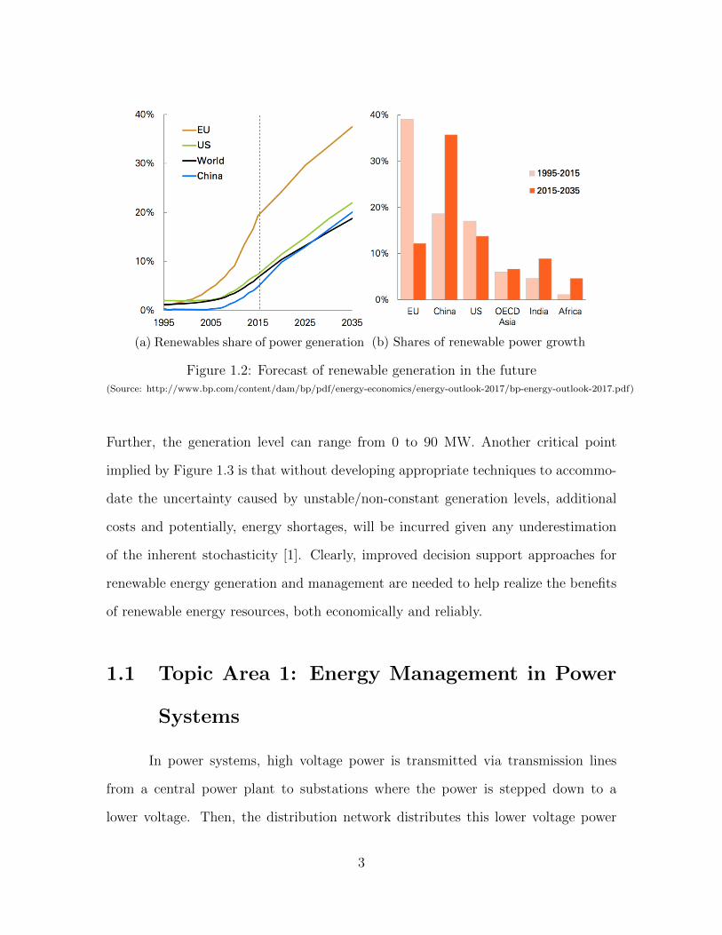
(a) Renewables share of power generation (b) Shares of renewable power growth

Figure 1.2: Forecast of renewable generation in the future(Source: http://www.bp.com/content/dam/bp/pdf/energy-economics/energy-outlook-2017/bp-energy-outlook-2017.pdf)

Further, the generation level can range from 0 to 90 MW. Another critical point

implied by Figure 1.3 is that without developing appropriate techniques to accommo-

date the uncertainty caused by unstable/non-constant generation levels, additional

costs and potentially, energy shortages, will be incurred given any underestimation

of the inherent stochasticity [1]. Clearly, improved decision support approaches for

renewable energy generation and management are needed to help realize the benefits

of renewable energy resources, both economically and reliably.

1.1 Topic Area 1: Energy Management in Power

Systems

In power systems, high voltage power is transmitted via transmission lines

from a central power plant to substations where the power is stepped down to a

lower voltage. Then, the distribution network distributes this lower voltage power

3

0 50 100 150 200 250 300Time (5 minutes)

0

10

20

30

40

50

60

70

80

90

100G

ene

ratio

n (

MW

)

Figure 1.3: Solar generation level during a day at (-118.85, 35.35)

to customers. Generating energy in large central plants saves capital costs per kW

of installed power. However, one drawback of the US’s current power grid is that

typically it relies on non-renewable resources that are environmentally unfriendly,

such as gas or coal. Another disadvantage inherent in the US’s large power grid is

the reality of transmission inefficiencies that result from long-distance transmission.

Further, when a part of the grid is affected due to maintenance actions or power

outages, the entire grid is impacted. To overcome all these drawbacks, microgrids,

which can improve efficiency, reliability, and security [2, 3], are emerging as alternate

sources of power generation. As defined by the US Department of Energy Microgrid

Exchange Group [4], “a microgrid is a group of interconnected loads and distributed

energy resources within clearly defined electrical boundaries that acts as a single

controllable entity with respect to the grid.”

A microgrid can be operated as part of a power system or in an islanded mode

in terms of connecting to or being disconnected from the main grid. When microgrids

4

are connected to a power grid (Figure 1.4), microgrids can either purchase power from

or sell power to the main grid. In addition, a microgrid can connect to neighboring

microgrids such that it can purchase power from or sell power to its neighbors. To

be able to sell power to the power grid or its neighbors, microgrids must have local

(distributed) energy generation.

In addition to conventional energy resources such as gas, diesel, and fuel oil,

the popularity of incorporating renewable energy resources into microgrids is evident,

as researchers have been focused on increasing renewable energy penetration in micro-

grids [5, 6, 7, 8, 9]. For example, the average annual renewable energy penetration in

Kodiak, Alaska, the second largest island in the US, has increased to 99.7% since the

Kodiak Electric Association first set a goal of 95% renewable resources penetration

in 2007.

PEV

HVAC

Appliances

PEV

Storage device

Storage deviceAppliances

Industrial facility(a)

(b)

(c)

(d)

Figure 1.4: An example of power system

5

According to the US Energy Information Administration, 37% of the nation’s

renewable energy was generated by wind and solar in 2014. Unfortunately, the in-

herent stochasticity in both the wind and the solar radiation can cause power grids

to become unstable as generation fluctuates with weather variations. As a result, if

the energy in microgrids is not managed efficiently, renewable energy resources can

increase microgrid operational costs. For example, if 1) microgrid renewable gener-

ation is insufficient to serve local users during time periods of high electricity prices

and 2) energy storage systems were not charged sufficiently during periods of low

electricity prices, then the microgrid must purchase energy from the power grid or

run local conventional generators to satisfy power demand—both of these options are

more expensive than using renewable generation.

With the development of the smart grid, which uses digital communication

technology to detect and react to local changes in power usage, end-use customers’

activities can be diverse as they can adjust their energy demands in response to

changes in electricity prices. For example, a household may choose to do laundry

at 3:00 pm rather than 7:00 pm if cheaper electricity prices prevail in the afternoon.

Such customer-driven demand response can benefit the power system by increasing

power system flexibility, helping to secure the power system by load curtailment and

shifting, and reducing costs by reducing generating capacity requirements. These

response activities, which are not only undertaken by households, but also by members

of the industrial and commercial sectors, need to be investigated further in the energy

management research.

Although a number of researchers have studied energy management in general,

no prior research investigates demand response in microgrids containing renewable en-

ergy resources that are connected to the main power grid. Given the importance of

and potential benefits resulting from this topic area, the first phase of my dissertation

6

research will focus on developing a stochastic optimization framework for coordinating

operations of the main power grid with multiple microgrids. Various energy manage-

ment settings (e.g., demand response) will be considered in the power system along

with the uncertainty of renewable energy generation. The goal of this research phase

is to provide models and solution methodologies that can help decision makers to

operate power systems efficiently and economically.

1.2 Topic Area 2: Production Scheduling with On-

site Renewable Energy in Industrial Plants

As one type of end-use customer of power systems, manufacturing plants typ-

ically purchase their needed power from the electricity grid to run productions. As

reducing production costs is one of the main goals of any manufacturing plant, ef-

fective scheduling, often plays a crucial role in most manufacturing and production

systems in achieving such the economic goals. Scheduling is performed at a vari-

ety of temporal levels. Medium-term scheduling allocates jobs to factories in specific

workweeks for completing expected customer orders, while short-term scheduling con-

siders allocation decisions for specific resources such as machines and people over a

short time horizon (e.g., a shift or a day) for actual customer orders. Scheduling

methods and algorithms typically focus on optimizing cost- and/or time-related ob-

jectives/performance measures.

In different manufacturing plants, the production environment can vary ac-

cording to the number of machines, machine types, speed, and/or layout configura-

tion, to name only a few types of variants. The simplest machine environment is a

single machine that processes individual jobs [10]. It can be thought of as a simplified

7

version of all other, more complicated machine environments, such as flow shops and

job shops [11, 12]. A flow shop consists of a set of m machines processing n jobs

such that each job has to follow the same route (machine order/sequence) during its

processing. Job shops are similar to flow shops in that jobs are processed by a number

of different machines according to a pre-specified sequence. However, in a job shop,

each job has its own unique, predetermined process route to follow.

While today’s production schedules minimize costs, we assert that they do

consider the electricity costs associated with production. With the development of

the smart grid, manufacturing plants are faced with additional challenges of accom-

modating electricity price-based programs to improve their production economics.

For example, the time-of-use electricity pricing schemes are designed to motivate cus-

tomers to use more energy at off-peak time periods. Under this scheme, users are

charged higher rates for consuming power at popular (peak) time periods when de-

mand is at its highest and cheaper rates at other time periods. Similarly, real-time

electricity pricing schemes are used by utilities to incentivize customers to shift their

energy demands from peak periods to low-demand periods, as electricity prices vary

hour-to-hour according to wholesale market prices.

A small number of research studies in the production literature focus on re-

ducing the environmental impacts caused by the emission of hazardous gases, such as

sulfur dioxide (SO2) and carbon dioxide (CO2), which are by-products of conventional

energy sources. Sulfur dioxide is one of the gases that caused London’s lethal smog in

the winter of 1952 [13]. The mortality rate for the smog period from December 1952

to February 1953 was remarkably high. Reducing the emission of such harmful gases

is another reason renewable and environment-friendly energy resources are receiving

attention from academics and practitioners alike. Given the intermittent nature of

renewable energy resources (e.g., the highest and lowest generation levels in Figure

8

1.3 are 90 MW and 0 MW, respectively), an excess (shortage) of power can occur

when demand levels are below (exceed) the available generated power. To increase

the utilization of renewable energy, batteries, which can store unutilized energy, com-

monly are used. Batteries can save conventional energy costs if they are charged when

there is an abundance of energy and electricity prices are low, and discharged when

power is needed and electricity prices are high.

Therefore. the second phase of my dissertation research will focus on inte-

grating production scheduling decisions with on-site renewable energy resources for

manufacturing processes in different machine environments. My research will capture

the stochasticity of renewable energy resources and comprehend the operations/usage

of energy storage systems while considering various electricity pricing schemes, such

as time-of-use and real-time pricing. The goal of this phase of my dissertation research

is to develop effective scheduling decision support algorithms for decision makers in

manufacturing plants that are considering renewable energy alternatives.

1.3 Research Contributions

The high cost and limited sources of fossil fuels, the global desire for clean en-

ergy resources, and the need to reduce carbon footprint have made renewable energy

resources attractive alternatives in both residential and industrial sectors. However,

the intermittent nature of renewable energy resources introduces challenges to full

power systems integration, given their uncertain generation schedules. These chal-

lenges are not only faced by power grids but also faced by end-use customers when

on-site renewable generation is one of their available energy supplies. My dissertation

research studied two different application areas of renewable energy resources: power

systems and end-use customers. The specific research contributions in my dissertation

9

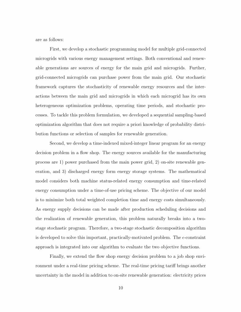
are as follows:

First, we develop a stochastic programming model for multiple grid-connected

microgrids with various energy management settings. Both conventional and renew-

able generations are sources of energy for the main grid and microgrids. Further,

grid-connected microgrids can purchase power from the main grid. Our stochastic

framework captures the stochasticity of renewable energy resources and the inter-

actions between the main grid and microgrids in which each microgrid has its own

heterogeneous optimization problems, operating time periods, and stochastic pro-

cesses. To tackle this problem formulation, we developed a sequential sampling-based

optimization algorithm that does not require a priori knowledge of probability distri-

bution functions or selection of samples for renewable generation.

Second, we develop a time-indexed mixed-integer linear program for an energy

decision problem in a flow shop. The energy sources available for the manufacturing

process are 1) power purchased from the main power grid, 2) on-site renewable gen-

eration, and 3) discharged energy form energy storage systems. The mathematical

model considers both machine status-related energy consumption and time-related

energy consumption under a time-of-use pricing scheme. The objective of our model

is to minimize both total weighted completion time and energy costs simultaneously.

As energy supply decisions can be made after production scheduling decisions and

the realization of renewable generation, this problem naturally breaks into a two-

stage stochastic program. Therefore, a two-stage stochastic decomposition algorithm

is developed to solve this important, practically-motivated problem. The ε-constraint

approach is integrated into our algorithm to evaluate the two objective functions.

Finally, we extend the flow shop energy decision problem to a job shop envi-

ronment under a real-time pricing scheme. The real-time pricing tariff brings another

uncertainty in the model in addition to on-site renewable generation: electricity prices

10

will impact the second-stage objective function in a two-stage stochastic program as

they are objective function coefficients. As most job shop scheduling problems are

known to be NP-hard, the computational time should prove unacceptably long for

solving this problem at any practical scale using commercial solvers. Therefore, we

develop a hybrid multi-objective evolutionary algorithm that integrates a mathemat-

ical approach with NSGA-II [89]. Five methods are developed to calculate fitness

value for the flow shop scheduling problem and commercial solver is used to compute

the optimal energy costs.

11

Chapter 2

Stochastic Optimization for Energy

Management in Power Systems

with Multiple Microgrids

S. Wang, H. Gangammanavar, S. D. Eksioglu, and S. J. Mason, “Stochastic opti-mization for energy management in power systems with multiple microgrids.” IEEETransactions on Smart Grid, vol. 10, no. 1, 1068-1079, 2019.

Nomenclature

Sets

N := 0, 1, 2, . . . , N, the set of agents (n = 0 is the main grid)

T := 0, 1, 2, . . . , T, set of discrete time decision epochs

In the following definitions, t ∈ T , n ∈ N will hold, unless otherwise mentioned.

Bn buses

Ln transmission lines

12

In interconnection lines connected the main grid and microgrid n,

n ∈ N \ 0

Gn conventional generators

Rn renewable generators

Dn demands

Dfn fixed demands

Dvn flexible demands

V in industrial facilities

Vhn buildings that have heating, ventilation, and air conditioning

systems

Vbn storage devices

Vpn plug-in electrical vehicles

Van home appliances

Subset Gni ⊆ Gn denotes conventional generators connected to bus i ∈ Bn. Similarly,

we have the subsets Rni and Dni.

Parameters

Dnjt fixed demand (MW), j ∈ Vfn

Dij total flexible demands (MW) required by industrial facility, j ∈

V in

Daj total flexible demands (MW) required by home appliances, j ∈

Van

Dhjt minimum level of demand (MW) required by heating, ventilat-

ing, and air conditioning system j ∈ Vhn

∆hjt flexible portion of demand (MW) adapted by heating, ventilat-

ing, and air conditioning system, j ∈ Vhn

13

Sj total demand required by PEV, j ∈ Vpn

cgnjt conventional generation cost per MW, j ∈ Gn

cbijt selling price of power per MW, (i, j) ∈ In

dpijt penalty for under-utilizing the power already purchased (per

MW), (i, j) ∈ In

drnit penalty for under-utilizing the renewable power (per MW), i ∈

Rn

d`nit penalty for unmet demand (per MW), i ∈ Dn

Avn feasible region for decisions anjt

Vnit voltage of bus i ∈ Bn

Xnij reactance of line (i, j) ∈ Ln

vn weight of agent n

aminj , amaxj bounds of utilized power (MW), j ∈ Dn

sminj , smaxj bounds of charging/discharging activities for storage devices

and plug-in electrical vehicles (MW), j ∈ Vbn ∪ Vpn

pminnij , pmaxnij bounds of power flow (MW) distributed by line (i, j) ∈ Ln

[τ ij, τij ] ⊆ T operation time interval for industrial facility j ∈ V in

[τ pj , τpj ] ⊆ T operation time interval for plug-in electrical vehicle j ∈ Vpn

[τaj , τaj ] ⊆ T operation time interval for home appliance j ∈ Van

ωnjt random variable, renewable generation (MW), j ∈ Rni

Decision Variables

bijt transaction power (MW) between the main grid and microgrid

n, (i, j) ∈ In, n ∈ N \ 0

gnjt conventional generation level (MW) at main grid, j ∈ Gn

anjt power (MW) utilized to meet demand, j ∈ Dn

14

snjt state of storage devices/plug-in electrical vehicles, j ∈ Vbn ∪ Vpn

pnijt power flow (MW) distributed by line (i, j) ∈ Ln

upjit unused purchased power (MW), (j, i) ∈ In

urnit unused renewable generation (MW), i ∈ Rn

u`nit unmet demand (MW), i ∈ Dn

θnit voltage angle of bus i ∈ Bn

2.1 Introduction

Microgrids have recently emerged as an alternative for reducing greenhouse

gas emissions and transmission losses [14, 15]. A microgrid (MG) is a small-scale

power grid that is comprised of distributed energy resource systems, storage devices,

local demands, and a distribution network [16, 17]. The capacity of such a distributed

energy resource system varies from 1500 kW to 1000 MW, which is smaller than a

centralized conventional power station [18]. Among all distributed energy resources

used in MGs, renewable energy sources (RESs), such as wind and solar, have obtained

more attention. Besides reducing greenhouse gas emissions, RESs are easy and eco-

nomical to obtain, especially in islands and outermost regions [8]. Many researchers

have investigated methods to increase the penetration of RESs in MGs such as using

storage devices [19]. However, the inherent stochasticity of renewable resources, such

as wind and solar, introduces operational challenges of MGs. An attractive feature of

MGs is their ability to operate both as part of a larger power grid [20, 21] as well as in

an islanded mode [8, 22]. MGs can transact power with the larger grid when they are

connected, thereby acting as a source/sink for deficient/excess power in the system.

In times of stress, such as during a storm or service interruption, an MG can break

off from the larger grid and operate independently on its own. These capabilities can

15

provide additional reliability options to power system operations. Energy managers

[16] at microgrids make generation decisions according to information provided by

local generation capacity, customer demand, and the amount of power transacted

with the main grid.

For these reasons, there has been a growing number of publications that focus

on the operations of MGs in the presence of renewable energy resources and/or stor-

age devices. These works have attempted to capture the interactions between MGs

and system operators. The setting in [20] was addressed using a simulation-based

testing method where economic dispatch decisions at MGs are solved in a primary

level and a secondary level optimization seeks to minimize overall operating costs.

In [21], TSO-DSO-MGs interactions are captured via an optimization problem that

is solved using diagonal quadratic approximation method and a variant of alternat-

ing directions method of multipliers. Networked MGs using a bi-level programming

model were presented in [23]. A deterministic equivalent mathematical program with

complementarity constraints of the bi-level program built using a scenario reduction

technique is proposed as a solution approach. In these studies, authors attempt to

optimize all MGs simultaneously, which can result in a large optimization problem. In

order to achieve computational viability, they consider only a small number of MGs

in the system and resort to a limited sample representation of uncertainty. However,

it is expected that in the future, the main grid will interact with a large number of

MGs. Alternatively, energy management in a multi-agent setting and in the context of

electricity markets has been studied by [24, 25, 26]. These problems are solved using

agent-oriented programming, Lagrangian-relaxation genetic algorithms, and a com-

bination of stochastic programming and game theory, respectively. Once again, these

works are limited to a small set of MGs to achieve computational viability. Moreover,

developing solution approaches that converge in uncertain problem settings is still an

16

area of active research. We adopt a stochastic programming approach to tackle some

of these issues. Stochastic programming has previously been applied successfully to

power system operation problems as they provide convenient tools to model com-

plicated interactions, physical restrictions, and uncertainties [27]. In our work, we

propose a novel approach to model this multi-agent setup and a sequential sampling

algorithm to solve this problem, which provide provably convergent solutions.

MGs allow integrating smart grid control systems and innovative energy man-

agement technologies with traditional operations. In a smart grid, customers are

allowed to adjust their energy consumption according to real-time electricity prices.

The adjustable appliances either have flexible ranges of power demand or can shift

their demand between periods. This behavior, which is called demand response,

brings operational flexibility while imposing newer challenges on energy management

systems. Most of adjustable demands considered in literature are storage devices and

plug-in electrical vehicles [19, 28, 29]. In [20] and [29], the authors provide math-

ematical models for general adjustable demand. However, the type of adjustable

demands varies including industrial, commercial, and residential. Ding et al. [30]

study non-schedulable and schedulable tasks in industrial facilities. Goddard et al.

[31] study heating, ventilation, and air conditioning demand response control in com-

mercial buildings. Li et al. [32] present detailed models of appliances commonly used

in households and investigates the optimal demand response schedule that maximizes

customer’s net benefit. Chen et al. [33] propose stochastic optimization and robust

optimization approaches for real-time price-based demand response management for

residential appliances. In this work, we propose a detailed mathematical model that

captures heterogeneous management systems with adjustable demands and incorpo-

rates physical power network restrictions.

In light of the above contents, the main contributions of this paper are:

17

1. A stochastic programming model that extends the classical two-stage formu-

lation to accommodate multiple subproblems. In the power systems context,

this model is designed for a centralized arbiter, who is charged with generating

and supplying power to a set of utilities and MGs with various weights (prior-

ities), in the main grid. Each MG is allowed to respond to the decision of the

centralized arbiter and a stochastic realization of renewable generation.

2. A comprehensive model that allows MGs to use different energy management

systems. This leads to heterogeneous agent optimization problems, operating

time periods, and stochastic processes. To the best of our knowledge, our work

is the first to consider such a setup.

3. An extension of the two-stage stochastic decomposition (2-SD) to solve models

with multiple subproblems. Our approach, which we refer to as the multi-agent

stochastic decomposition, is a decomposition-based sequential sampling algo-

rithm. It dynamically identifies the number of samples required to characterize

the uncertainty at a particular MG and provides statistically verifiable solutions

and objective function estimates.

4. A comprehensive computational analysis that highlights the scalability of the

proposed algorithm to large-scale power systems. The results of our analysis

illustrate the performance of the algorithm, the benefits of energy management

systems, and the advantages of flexible demands.

The remainder of the chapter is organized as follows. In Section 2.2, the energy

management in power systems is studied and corresponding mathematical model is

presented. The multi-agent stochastic decomposition is implemented in Section 2.3.

Computational experiments are conducted in Section 2.4. Finally, conclusions are

18

offered in Section 2.5.

2.2 Problem Formulation

We consider a power system that is comprised of a main grid connected to

multiple agents. The main grid can either be a transmission or distribution net-

work. In transmission networks, the independent system operator (ISO) acts as the

centralized arbiter bestowed with the responsibility of managing not only the opera-

tions (generation, transmission, etc.) of the transmission network, but also managing

the transactions with distribution networks and MGs connected to it. The agents

themselves are managed by autonomous decision-making entities (distribution sys-

tem operators (DSO) for distribution networks and energy management systems for

MGs). Similarly, the distribution system operator shares the same interactions with

MGs connected to the distribution network. While the role of decision makers at

individual agents is concerned with the operations on a small/local scale, the central-

ized arbiter is interested in optimal operations of the entire system. The formulation

presented in this section encompasses any such relationship between the centralized

arbiter and agents. In the remainder of the paper, we will restrict all agents to be

MGs with independent energy management systems controlling their operations.

The power system uses both conventional and renewable energy resources to

meet customer demands. Each entity in the system is exposed to varied sources

of uncertainty (demand, renewable generation, etc.) and utilizes different energy

management settings. Fig.2.1 shows the system we described above. To capture

these properties of the system, we present a stochastic optimization formulation that

is comprised of (a) an arbiter problem where decisions are made before the realization

of any uncertainty and (b) multiple agent problems where decisions are made in

19

MG2

(PEVs,HVAC)

MG1

(Homeappliances,PEVs,

Storagesdevice)

MGn

(Industrialfacility,Storage

device)

Main grid(a)

(b)

(c) (d)

Figure 2.1: A power system: A main grid (a) connects to multiple MGs ((b) - (d))that utilize different energy management settings

response to their respective stochastic outcomes. This formulation is an extension of

the classical 2-SP and will be referred to as the multi-agent stochastic program (MA-

SP). At time period t, customer demands at each agent can be met through local

generation (conventional and renewable) as well as energy bought from the main grid

(when n 6= 0). We first begin by presenting the arbiter’s optimization problem.

2.2.1 Arbiter Problem

The centralized arbiter determines the conventional generation level at the

main grid as well as its power transactions with all the MGs. The set of generators

in the main grid is denoted by G0. For every generator j ∈ G0, the generation level

and the corresponding cost are denoted by g0jt and cg0jt, respectively. The transaction

decisions bijt between the main grid and MGs are determined for all (i, j) ∈ In at

a price of cbijt, where In is the set of interconnection links. These generation and

transaction decisions are made so as to satisfy the following power balance equation:

∑j∈G0

g0jt =∑

j∈D0⋃R0

∂D0jt +∑

(i,j)∈In

bijt ∀t ∈ T , (2.1)

20

where ∂D0jt is the net demand computed using the forecasted demand (D0) and

renewable generation (R0) in the main grid. In addition, generation and transaction

decisions are bounded by their respective physical limits. Further, these decisions are

established in a “here and now” manner and effect the state of every agent in the

system. We will succinctly denote the arbiter’s decision vector by x = (xt)t∈T and

cost vector by c = (ct)t∈T , where xt = ((g0jt)j∈G0 , (bijt)(i,j)∈I) and the corresponding

cost coefficients by ct = ((cg0jt)j∈G0 , (−cbijt)(i,j)∈I). The feasible set characterized by

(1) is denoted by X . Once the arbiter makes its decision, each agent responds to this

decision and a realization ωn of its stochastic process ωn at a recourse cost of hn(x, ωn).

We assume that the stochastic processes affecting the agents are independent of each

other.

The objective of the centralized arbiter is to minimize the energy cost and the

sum of weighted expected recourse functions. Its optimization problem is given by:

min c>x+∑n∈N

vnEhn(x, ωn)

s.t. x ∈ X , (2.2)

where the weight vn ≥ 0 ∀n ∈ N is chosen based on the relative preference of the

agents set by the centralized arbiter. For example, an agent with critical infrastruc-

tures (like hospitals) has higher priority (weight) than other agents.

2.2.2 Agent problem

Each agent in the system, that is, the main grid and all MGs, is associated

with an agent problem. This problem is characterized by the energy management

setting adopted and stochasticity faced by the agent. The energy resources of an

21

agent n include the set of conventional generators Gn as well as renewable generators

Rn. The conventional generators at MGs (n 6= 0) usually have lower capacities when

compared to the main grid (n = 0) generators. In addition to these local energy

resources, the MGs can utilize a fraction of the energy available from the main grid.

The generation levels g0jt ∀j ∈ G0 at the main grid, which were set by the arbiter,

are allowed to be updated.

These resources are used to meet customers’ demands, which are denoted by

Dn. Further, all customer demands can be categorized as fixed and flexible. The

fixed demand, Dnjt, at location j ∈ Dfn must be met in the current time period t. In

other words,

anjt ≥ Dnjt, (2.3)

where anjt is the power utilized to meet this fixed demand. The flexible demand, Dvn,

depends on the energy management settings adopted by each agent. We will describe

these settings in the following.

2.2.2.1 Energy Management Settings

Each agent may adopt (one or more) different settings. Therefore, we omit

the agent index n while presenting these settings.

1. Industrial Sector: The field of production management provides flexibility in

how demand at a particular facility can be met during the operation time

horizon[30]. This, in turn, allows for efficiently utilizing the available energy

resources. To ensure that the production demand is met, the cumulative power

consumption within a production window must exceed a given threshold. Let

V i denote a set of industrial facilities. If for each j ∈ V i, the time window

within which the demand Dij can be satisfied is given by [τ ij, τ

ij ] ⊆ T . This

22

requirement is captured by:

∑t∈[τ ij ,τ

ij ]

ajt ≥ Dij. (2.4)

In the above, ajt is the realized power in time period t that is restricted to be

within an interval [aminj , amaxj ] ∈ R. The equipment used in industrial settings

is associated with significant start-up time and set-up cost. Therefore, it is

efficient to run the industrial equipment uninterrupted, which is ensured by

setting aminj > 0.

2. Building Management: For commercial buildings, around 50% of the energy is

consumed by heating, ventilation, and air conditioning (HVAC) systems to pro-

vide a comfortable indoor environment [34]. Let Vh denote the set of buildings

that have intelligent HVAC systems. Since comfort is a qualitative term, it is

best captured through a flexible range. For example, the comfortable indoor

temperature ranges between 20C to 25C [35]. Moreover, this comfort is also

associated with climate [36] and building occupancy [37]. For these reasons, the

amount of energy consumed has a fixed minimum level Dhjt (corresponding to

the minimum comfort requirement) and a flexible portion ∆hjt for all j ∈ Vh.

The flexible portion can frequently fluctuate within a range without reducing

the end-user’s comfort significantly. This is ensured by:

Dhjt ≤ ajt ≤ Dh

jt + ∆hjt ∀j ∈ Vh,∀t ∈ T . (2.5)

Note that, while the demand in (2.4) can be met across multiple time periods,

the demand here is time-dependent and should be met in its time period.

23

3. Storage Devices: It has been identified that storage devices will play a critical

role in mitigating renewable regulation challenges [38, 39]. Apart from energy

arbitrage, storage devices can provide ancillary services, capacity deferral ser-

vices, and end-user services [40]. Let Vb denote a set of storage devices. For

each j ∈ Vb, ajt is the charging/discharging amount during time period t. If

this value is positive, it indicates a charging activity—discharging otherwise.

These decisions are bounded by charging/discharging rates of the storage de-

vices: ajt ∈ [aminj , amaxj ] ∈ R. Let sjt denote the state of storage devices that is

required to satisfy the following dynamics equation:

sjt = sj,t−1 + ajt ∀j ∈ Vb, ∀t ∈ T , (2.6)

where the initial state sj0 is assumed to be given. This variable is also bounded

by the capacity of this storage device, that is 0 ≤ sjt ≤ smaxj . In any time

period, a storage device can act both as source and sink of energy.

4. Plug-in Electric Vehicle (PEV): The operating principle of PEVs is similar to

that of storage devices. However, unlike the storage devices, the charging and

discharging activities depend on the utility of the vehicle. For example, it should

be expected that the PEVs are connected to a residential grid during the off-

work hours. Therefore, the whole operation must be completed during a time

period that is desired by the customer. Using similar definitions as given for

storage devices, for j ∈ Vp, the set of PEVs must satisfy:

aminj ≤ ajt ≤ amaxj , sminj ≤ sjt ≤ smaxj (2.7a)

sjt = sj,t−1 + ajt ∀t ∈ [τ pj , τpj ], (2.7b)

24

where [τ pj , τpj ] is the plug-in interval. Further, the state of the PEVs at the end of

the plug-in interval must satisfy the specific customer-desired requirement[33]:

sjτpj = Sj ∀j ∈ Vp. (2.8)

5. Home Appliances: The operation of some appliances, such as dishwashers and

washing machines, is flexible over a time horizon. These appliances have rela-

tively lower demand compared to the other settings described thus far. Let Va

denote a set of appliances. For each j ∈ Va, ajt is the power utilized in time

period t that must satisfy:

∑t∈[τaj ,τ

aj ]

ajt ≥ Daj (2.9)

during the desired time window [τaj , τaj ]. The operation of these appliances can

withstand interruptions since the start-up time and set-up cost are negligible.

Moreover, power utilized in any time period should be less than the power rating

of the appliance. Therefore, ajt ∈ [0, amaxj ]. The interruptible nature of these

appliances differentiates them from industrial equipment.

We restrict our attention to the above five settings, but other similar settings

can also be operated within our multi-agent framework. Moreover, for agent n the

flexible demand set Dvn can be any combination of the above settings. The feasible re-

gion for decisions anjt, where j ∈ Dvn depends on this combination and will be denoted

as Avn. For example, for a household with storage devices and PEV units installed,

the set Dvn = Vbn⋃Vpn⋃Van. In this case, the feasible region Avn is characterized by

(6), (7), (8), and (9) along with the respective bounds.

25

2.2.2.2 Power Network Constraints

The power grid in both the main grid and MGs (i.e., for all n ∈ N ) consists

of buses and lines that construct a network with a set of buses Bn and a set of

transmission lines Ln. At any bus i ∈ Bn, the total available power should meet the

total of fixed and flexible demands, thus, satisfying the following:

∑j∈Gni

gnjt +

( ∑j:(j,i)∈Ln

pnjit −∑

j:(i,j)∈Ln

pnijt

)−∑j∈Dni

(anjt − u`njt) = ri(xt, ωnit) ∀t ∈ T , (2.10)

where pnjit and pnijt are the flow into and out of bus i, respectively. Further, ujit

is the purchased power that is unused. Note that this variable appears only in MG

problems. The right-hand side ri(xt, ωnit) depends on the arbiter’s decision and the

renewable generation ωnit. Note that the right-hand side ri(xt, ωnit) for the main grid

and MGs are different since the main grid acts as a seller rather than a buyer in

the transactions with agents. Therefore, for any bus i ∈ Bn, ri(xt, ωnit) is set as the

following:

−∑j∈Rni

(ωnjt − urnjt) +∑

j:(i,j)∈In

bijt if n = 0,

−∑j∈Rni

(ωnjt − urnjt)−∑

j:(j,i)∈In

(bjit − upjit) if n 6= 0.

(2.11)

On any transmission line, the real transmitted power and power losses are non-

linear functions of the differences between the voltages and angles of buses in both

ends of connecting lines. To make these functions suitable for linear optimization

methods, we apply a linear approximation described in [41]. We ignore the power

flow losses. If Vnit denotes the voltage of bus i, and Xnij denotes the reactance of line

26

(i, j) ∈ Ln, then the power flow pnijt is given by:

pnijt =VnitVnjtXnij

(θnit − θnjt) ∀t ∈ T , (2.12)

where the decision variable θnit is the angle of bus i. Further, the power flow pnijt

and bus angle θnit should be within their intervals [pminnij , pmaxnij ] and [θminnij , θ

maxnij ], re-

spectively.

Each agent has the objective of minimizing the following: the total cost of

generation, the penalty for under-utilizing the power already purchased, the unused

renewable generation, and the unmet demands. Let cgnjt, dpijt, d

rijt, and d`ijt represent

the corresponding unit costs, thus, the objective is:

hn(x, ωn) = min∑t∈Tn

[∑j∈Gn

cgnjtgnjt +∑

(i,j)∈Inn6=0

dpijtupijt+

∑j∈Rn

drnjturnjt +

∑j∈Ln

d`njtu`njt]

s.t. (2.3), (2.10), and (2.12)

anjt ∈ Avn. (2.13)

The arbiter’s decision as well as stochastic information (renewable generation)

affect only the right-hand side of the above program. The agent subproblem and the

arbiter’s problem in (2.2), which is referred to as the first-stage problem, together

constitute our MA-SP:

min c>x+∑n∈N

vnEhn(x, ωn) (2.14a)

s.t. x ∈ X ,

27

where,

hn(x, ωn) = min d>n yn (2.14b)

s.t. Wnyn ≤ rn(ωn)− Tn(ωn)x,

yn ≥0.

The subproblem (2.14b) is a succinct representation of the agent problem in (2.13).

We resort to this representation to simplify the exposition of our algorithm in the

next section. Notice that the objective function and constraints are linear functions,

the first-stage decisions affect the right-hand side of (2.14b), and the recourse matrix

is independent of uncertainty. Therefore, this formulation is an extension of 2-SP

with fixed recourse [1].

2.3 Algorithm

The formulation introduced in Section 2.2 has an arbiter problem where de-

cisions are made before the realization of demand and renewable generation as well

as multiple agent problems that provide the recourse costs for the arbiter’s decisions.

If all the agents can be operated/controlled by a single decision maker, then a com-

bined optimization program can be used to obtain their decisions (shown by the large

shaded blue box in Figure 2.2a). Further, a subproblem scenario is a single vector

of observation at all agents. In this setting, the problem can be formulated as a

2-SP. However, the agents have independent decision makers with heterogeneous op-

timization problems. They are exposed to different stochastic processes. As (2.14)

shows, the proposed MA-SP has a weighted sum of expected recourse functions in

the first stage. Each expected recourse function corresponds to an independent agent

28

Combinedagent1,agent2,…,agentnsubproblem

Second stage

( ) ( ) ( )

Arbitermaster

problem

First stage

( )Scenario for the subproblem

(a) Decision structure of 2-SP

Scenario for Agent 1

Scenario for Agent 2

Scenario for Agent 3

Arbiter master

problem

Agent1 Agent2 Agentn

First stage

Second

stage

(b) Decision structure of MA-SP

Figure 2.2: Decision structures

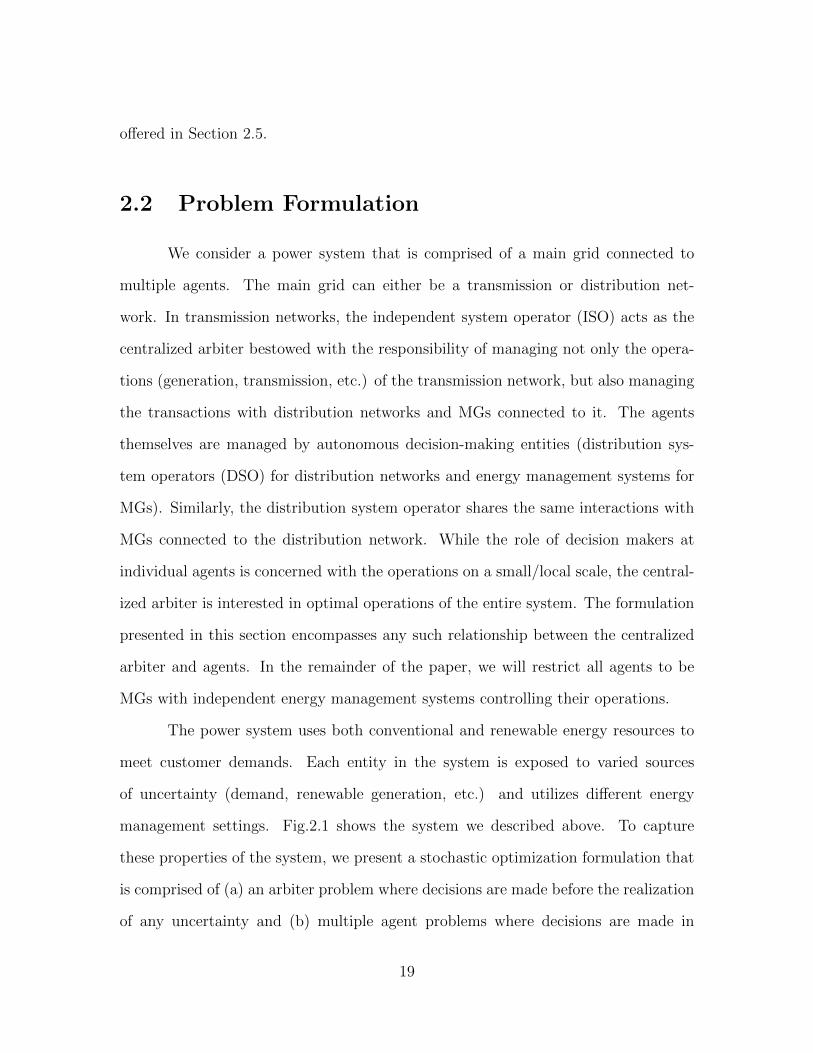
subproblem (shown by separate and small shaded blue boxes in Figure 2.2b). In this

case, every agent only observes scenarios from its stochastic process. The presence of

multiple subproblems distinguishes our MA-SP from the classical formulation which

only has one expected recourse function.

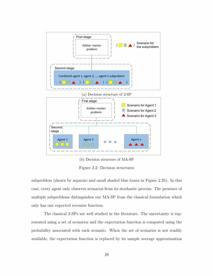
The classical 2-SPs are well studied in the literature. The uncertainty is rep-

resented using a set of scenarios and the expectation function is computed using the

probability associated with each scenario. When the set of scenarios is not readily

available, the expectation function is replaced by its sample average approximation

29

(SAA):

H(x) =1

M

M∑i=1

h(x, ωi), (2.15)

where M is the number of scenarios. Several algorithms, notably, Benders’ decom-

position [42], Dantzig-Wolfe decomposition [43], and progressive hedging [44], can

be used to solve the SAA. These algorithms build lower bounding piecewise linear

functions by solving a subproblem for each scenario from a set of scenarios selected a

priori. For large-scale problems and/or problems with a large set of scenarios, such

enumeration can prove to be computationally challenging. This is particularly the

case in power systems with significant renewable integration. For such problems,

sequential sampling-based bundling algorithms, such as 2-SD, have proven to be ef-

fective [45]. Recent work [46] has illustrated the advantages of sequential sampling

over SAA for a wide range of applications. Motivated by these observations, we adopt

a modified 2-SD solution approach to tackle our MA-SP.

Our solution approach, which we refer to as multi-agent stochastic decom-

position (MA-SD), is an extension of 2-SD when multiple subproblems exist. The

principal idea is to use a separate sample mean function to approximate the expected

recourse function for each agent in (2.2):

Hkn(x) =

1

k

∑j∈Ωk

n

hn(x, ωjn) ∀n ∈ N . (2.16)

Note that the above sample mean is based on the current set of observations Ωkn. In

any iteration k, these sample mean functions are updated by sequentially sampling

scenarios (ωkn) from their respective stochastic processes and updating the observation

set Ωkn. For the current arbiter decision xk and newly sampled observation ωkn, the

subproblem for agent-n is solved. Let πkkn denote the corresponding optimal dual

30

solution. This solution is added to the set of previously encountered dual solutions,

Πkn. For the remaining observations ωjn ∈ Ωk

n, a dual solution πkjn is identified in Πkn,

which provides the best lower bound at xk. Using these dual solutions πkjn kj=1, we

compute a lower bounding affine function for the kth sample mean function Hkn(x):

Hkn(x) ≥ 1

k

k∑j=1

(πkjn )>[rn(ωjn)− Tn(ωjn)x]︸ ︷︷ ︸:= `kn(x,Ωk

n)

. (2.17)

Note that Hkn(x) approaches the expectation function as k →∞. Further, the affine

function `jn computed in iteration j(< k) is a lower bound for Hjn, and not necessarily

for Hkn.

Therefore, the previously generated affine functions are updated by multiply-

ing `jn by the factor jk. Using these, the piecewise linear approximation [47] of the

expected recourse function of agent n is given by:

Lkn(x) = maxj=1,...,k

j

k× `jn(x,Ωk

n)

. (2.18)

Approximations of (2.18) are weighted and aggregated across all agents to

form the first-stage problem, which is given by

min c>x+N∑n=1

vnLkn(x) +

σk

2||x− xk||2 |x ∈ X, (2.19)

for a given parameter σk > 0. The optimal solution of the above problem xk+1 will

be used in the subsequent iteration. Notice the use of a regularization term, centered

around the incumbent solution xk, in the objective function. This term is included

to stabilize our sampling-based approach. We refer the reader to [46] for a detailed

31

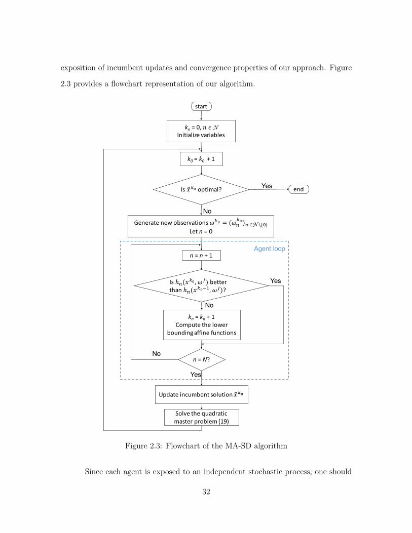
exposition of incumbent updates and convergence properties of our approach. Figure

2.3 provides a flowchart representation of our algorithm.

!"#$"

!" %&'(&!"#"N

)*+"+#,+-.&/#$+#0,.!

1.*.$#".&*.2&30!.$/#"+3*!&$%& ' ($)%&*)"+N ,-./

4."&" %&'

)!&01%& 35"+6#,7&

" %&" 8&9

)!&2)(0%& 3 $4* 0."".$&

":#*&2)(0%&563 $4*7&&&&&&&&&&&&&&&&

!" %&!" 8&9

;365<".&":.&,32.$&

03<*=+*>&#??+*.&?<*@"+3*!

" %&#7

.*=

A5=#".&+*@<60.*"&!3,<"+3*&01%&

B3,/.&":.&C<#=$#"+@&

6#!".$&5$30,.6&D9EF

!"#

$%

$%

$%

!"#

!"#

!$ %&!$% 8&9

&'"()*+%%,

Figure 2.3: Flowchart of the MA-SD algorithm

Since each agent is exposed to an independent stochastic process, one should

32

expect that different number of scenarios is required to characterize the uncertainty.

Further, since the optimization problem is different at every agent, the number of

extreme points (dual solutions) relevant to approximate the cost function is also dif-

ferent. In this regard, our stopping rules are based on in-sample as well as out-sample

tests for stability of the observation set Ωkn and dual solution set Πk

n. We refer the

reader to [46] for more details. Due to the heterogeneous nature of decision processes,

different agents might satisfy the stopping criteria at different iterations. Further,

since the algorithm allows samples to be added sequentially during the optimization

process, such a sequence can be obtained from state-of-the-art simulators that are

often used by power system operators.

2.4 Computational Experiments

For our computational experiments, we used the WECC-240 data set obtained

from [48]. The data consists of a detailed description of network topology, genera-

tor location, and capacity. In the data set, all 240 buses, which are located in the

western part of the U.S., are originally partitioned into 21 areas (see Figure 2.4). We

decomposed this data set into one main grid (shown in gray) connected to N = 10

MGs (shown in blue). The renewable generation data was extracted from the Western

Wind and Solar Integration Study [49] based on the generators’ geographical loca-

tions. This data was scaled to ensure 15% renewable penetration at each MG and

used to build a model that provides a stream of simulated outcomes for renewable

generation. We used the demand data in the WECC data set to create the instance,

and the buses with flexible demand were selected randomly from the set of all load

locations. We adopted the generation costs provided by [50]. Table 2.1 presents the

details of this power system. In our computational study, we set the time horizon

33

6

5

3

1

9

15

20

19

18

17

4 2

714

10

8

11

21

1216

13

Figure 2.4: Network toplogy of WECC-240

T = 24 hours.

All algorithms were implemented in the C programming language on a 64-bit

Intel core i7-4770 CPU @3.4GHz × 8 machine with 32 GB Memory. All linear and

quadratic programs were solved using CPLEX callable subroutines. In all our exper-

iments, we begin by using an optimization process to identify an optimal solution

for the arbiter and the corresponding prediction value. Note that this prediction

value is an estimate of the lower bound for the original optimization problem. This

is followed by a verification phase where the arbiter’s solution is fixed, and agents

(MGs) subproblems are simulated using independent and identically distributed ob-

servations. The objective functions obtained are used to build a confidence interval

(CI) of the upper bound estimate for each agent’s expected recourse function. The CI

for the arbiter objective function value is the aggregate based on the weighted sum

of individual agent objective values.

34

Tab

le2.

1:D

etai

lsof

the

WE

CC

-240

pow

ersy

stem

Age

nt

Wei

ghts

#B

use

s#

Lin

es#

Gen

erat

ors

#D

eman

dL

oca

tion

sE

ner

gyM

anag

emen

tSet

tings

nv n

|Bn|

|Ln|

|Gn||R

n|

Fix

ed(|D

f n|)

Fle

xib

le(|D

v n|)

|Vi n||V

h n||V

b n||V

p n||V

a n|

01

8110

024

040

00

00

00

11

2124

153

76

21

11

1

21

21

21

01

00

00

1

31

1518

21

57

21

12

1

41

1417

31

37

21

02

2

51

2936

51

1211

31

23

2

61

3341

167

510

31

12

3

71

65

51

03

20

00

1

81

2936

174

1110

23

13

1

91

54

31

12

00

01

1

101

55

31

13

10

01

1

35

2.4.1 Comparison of Decision Structures

We start by comparing our MA-SP with the classical 2-SP. While MA-SP

includes a separate subproblem for each agent, the 2-SP considers a subproblem that

aggregates together the decision processes of all agents. The uncertainty in 2-SP

is captured by a single random vector, say ωt = (ω1t, ω2t, . . . , ωNt). The first-stage

problem in both these formulations remains the same. We used the 2-SD algorithm

to optimize the 2-SP. These results are summarized in Table 2.2.

Note that the total costs (i.e., prediction value) for MA-SP is within 0.5% of

that predicted by the benchmark 2-SD algorithm. This indicates that the objective

function value estimated by considering a separate sampling procedure for each agent

is statistically similar to when a single stream of samples is used. The verification

CIs, on the other hand, provide us with a tool to compare the solutions generated

from the formulations. We accomplished this by testing the following hypothesis: the

solutions from the two formulations are statistically indistinguishable. The p-value

associated with this hypothesis test is 0.7008, which is greater than 0.05. It indicates

that the hypothesis cannot be rejected at a 0.95 significance level.

The first column of Table 2.2 shows that solving an MA-SP requires a smaller

number of iterations than solving a 2-SP (670 vs. 708). In 2-SP, the number of

Table 2.2: Comparison between 2-SP and MA-SP

Structure

# of

optimization

programs

Time per

iter.

(s)

Prediction

value

($)

95% C.I. p-value

2-SP 708 18.682 43,760,652[43,499,527,

44,103,080]-

MA-SP 670 9.849 43,951,145[43,534,253,

44,252,131]0.7008

36

scenarios (of random vector ωt) is equal to the number of optimization programs,

while, for solving the MA-SP, the number of scenarios encountered by each agent

(i.e., random variable ωnt) is different. We will discuss it in the following sub-section.

The average time taken to complete an iteration of each algorithm is presented in

Table 2.2 as well. Since MA-SP decomposes the subproblems into smaller linear

programs, the computational requirements are lower when compared to 2-SP where

a significantly larger linear program is solved. Therefore, the average time taken

for an iteration in 2-SD is twice as much as MA-SD. The separation of sampling

procedures and the computational advantage make the MA-SP setup suitable for

parallel computing environments. We are currently working on an implementation

suitable for such environments, and the results will be reported in future publications.

2.4.2 Comparison of Cut Formation Procedures

The expected recourse function for each agent is approximated using lower

bounding affine functions as described in Section 2.3. These approximations are

included in the master problem as linear functional constraints [51]. This implies

that the size of the master problem grows by N (number of agents/MGs) in every

iteration that increases the computational burden of solving quadratic programs.

Alternatively, one may aggregate these affine functions as:

α =N∑n=1

vnαn; β =N∑n=1

vnβn, (2.20)

where (αn, βn) are coefficients of individual affine functions for n = 1, . . . , N , and

(α, β) are those for the aggregated affine function. This choice motivates the next

set of experiments where we compare the MA-SD(m) and MA-SD(a) procedures. In

MA-SD(m), N affine functions are added in every iteration, and a single aggregated

37

function is added in MA-SD(a). The results of MA-SD(a) and MA-SD(m) are shown

in Table 2.3 and Table 2.4, respectively.

These results indicate that, while the number of quadratic master programs

solved is higher in the case of MA-SD(a) when compared to MA-SD(m), the cor-

responding running time is lower. This can be attributed to the larger size of the

master problem in the MA-SD(m). As before, we can compare the prediction and

verification values to establish the similarity between the two approaches. The differ-

ence in prediction values of the two approaches is around 0.3%. We also conducted a

hypothesis test that there is no difference between the solutions obtained from these

two algorithms. The p-value of 0.9751 (> 0.05) indicates that we cannot reject the

null hypothesis of statistically indistinguishable arbiter solutions.

The results in the two tables showcase one of the principal features of our solu-

tion approach, viz. the distributed nature of our sequential sampling procedure. Since

each agent is exposed to stochastic processes with different characteristics (mean, vari-

ance, etc.), the number of samples required to satisfactorily approximate the expected

recourse function is also different. These numbers can be seen in the first column of

Table 2.3 and Table 2.4 for each method, respectively. For sample-based stochas-

tic programming models, it is not guaranteed that the prediction value falls within

the verification CI. However, when it does, then the solutions can be accepted with

greater confidence. The arbiter solution satisfies this condition as the aggregated

prediction value falls within the verification CI for both methods proposed. (See the

row corresponding to “master” in Table 2.3 and Table 2.4.) While this solution is

statistically acceptable to the aggregated optimization problem, it might not be the

case for individual agents (e.g., agent 4 in the MA-SD(a) method). Such behavior can

be attributed to the fact that our approach seeks solutions that are optimal across

all and not necessarily individual agents. In the remaining experiments, we will use

38

Tab

le2.

3:R

esult

sof

MA

-SD

(a)

Age

nts

#of

opti

miz

atio

n

pro

gram

s

Tim

ep

er

iter

.(s

)

Pre

dic

tion

valu

e($

)M

ean

U.B

.E

stim

ate

Std

.dev

.95

%C

.I.

mas

ter

670

9.84

943

,951

,145

43,8

93,1

925,

788,

250

[43,

534,

253,

44,2

52,1

31]

036

90.

012

0.00

70.

007

0.00

0[0

.007

,0.

007]

130

10.

002

8,99

8,94

88,

997,

077

150,

725

[8,9

87,7

30,

9,00

6,42

4]

247

50.

002

8,75

58,

749

694

[8,7

06,

8,79

2]

335

90.

004

2,13

9,07

82,

140,

098

91,6

29[2

,134

,416

,2,

145,

780]

434

30.

004

2,07

6,82

21,

994,

509

946,

845

[1,9

35,7

93,

2,05

3,22

4]

536

80.

015

783,

400

772,

364

310,

294

[753

,122

,79

1,60

6]

627

50.

014

4,26

3,63

44,

205,

003

2,86

3,42

3[4

,027

,438

,4,

382,

569]

737

40.

003

5,22

8,60

35,

350,

485

4,56

0,16

9[5

,067

,701

,5,

633,

268]

826

50.

006

6,69

2,12

66,

665,

261

1,82

2,69

9[6

,552

,233

,6,

778,

290]

932

30.

001

206,

019

203,

565

101,

432

[197

,275

,20

9,85

5]

1035

10.

002

645,

443

640,

605

220,

237

[626

,947

,65

4,26

2]

39

Tab

le2.

4:R

esult

sof

MA

-SD

(m)

Age

nts

#of

opti

miz

atio

n

pro

gram

s

Tim

ep

er

iter

.(s

)

Pre

dic

tion

valu

e($

)M

ean

U.B

.E

stim

ate

Std

.dev

.95

%C

.I.

mas

ter

435

15.9

5744

,066

,906

43,8

85,1

095,

796,

994

[43,

525,

628,

44,2

44,5

91]

031

10.

012

0.00

40.

004

0.00

0[0

.004

,0.0

04]

127

90.

002

8,65

7,52

18,

654,

370

142,

600

[8,6

45,5

27,

8,66

3,21

3]

243

30.

002

8,82

48,

790

723

[8,7

45,

8,83

4]

337

50.

003

2,14

4,47

92,

146,

895

98,5

48[2

,140

,784

,2,

153,

006]

434

60.

004

2,05

3,00

82,

008,

981

958,

127

[1,9

49,5

66,

2,06

8,39

6]

539

30.

019

800,

002

774,

888

311,

272

[755

,585

,79

4,19

0]

626

70.

017

4,42

6,20

74,

213,

061

2,87

0,70

8[4

,035

,044

,4,

391,

078]

731

40.

002

5,17

3,33

75,

341,

604

4,56

0,19

4[5

,058

,819

,5,

624,

389]

826

30.

007

7,02

5,17

16,

965,

143

1,83

0,95

7[6

,851

,602

,7,

078,

684]

931

70.

001

197,

412

192,

457

92,5

95[1

86,7

15,

198,

199]

1028

10.

001

648,

653

646,

629

222,

103

[632

,856

,66

0,40

2]

40

MA-SD(a) as our method of choice to solve MA-SPs.

2.4.3 Study the Impacts of the Network Constraints

The formulation presented in Section 2.2 considers a DC approximation of the

power flow constraints (2.10). Power flow on line (i, j) is bounded by the line capacity

[pminnij , pmaxnij ]. In order to study the impact of these constraints, we created instances

without power flows (“NoNetwork”), uncapacitated power flows (“Uncapacitated”),

and capacitated power flows (“Capacitated”). In the “NoNetwork” instance, system-

wide power balance was ensured by including:

∑j∈Gn

gnjt =∑

j∈Dn⋃Rn

∂Dnjt −∑

(i,j)∈In

bijt ∀t ∈ Tn, (2.21)

where ∂Dnjt is the net demand computed using customer demand (Dn) and renewable

generation (Rn) in all agents n ∈ N . The results are shown in Table 2.5. Since the

“NoNetwork” and “Uncapacitated” instances are relaxations of the original problem,

the total cost is lower than the “Capacitated” instance. Moreover, the solution ob-

tained for “Capacitated” is significantly different from the other instances (indicated

by low p-value). It is interesting to notice that the solutions and values from “NoNet-

work” and “Uncapacitated” instances are statistically indifferent. This indicates that

the capacity on power flows is more critical than the power flow approximation (2.12),

at least for our data set.

2.4.4 Energy Management Study

The formulation of the power system presented in Section 2.2 permitted dif-

ferent energy management settings to be included at agents. A main feature of these

41

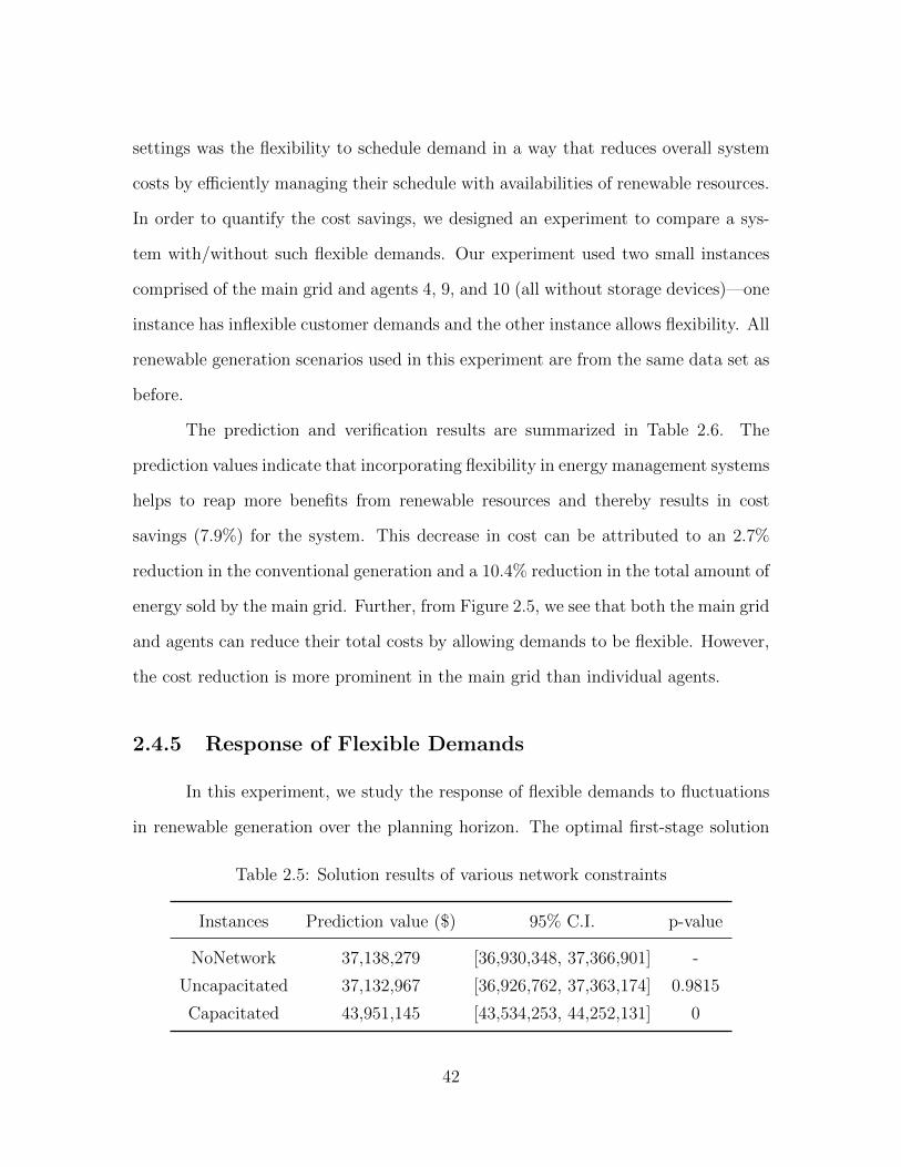
settings was the flexibility to schedule demand in a way that reduces overall system

costs by efficiently managing their schedule with availabilities of renewable resources.

In order to quantify the cost savings, we designed an experiment to compare a sys-

tem with/without such flexible demands. Our experiment used two small instances

comprised of the main grid and agents 4, 9, and 10 (all without storage devices)—one

instance has inflexible customer demands and the other instance allows flexibility. All

renewable generation scenarios used in this experiment are from the same data set as

before.

The prediction and verification results are summarized in Table 2.6. The

prediction values indicate that incorporating flexibility in energy management systems

helps to reap more benefits from renewable resources and thereby results in cost

savings (7.9%) for the system. This decrease in cost can be attributed to an 2.7%

reduction in the conventional generation and a 10.4% reduction in the total amount of

energy sold by the main grid. Further, from Figure 2.5, we see that both the main grid

and agents can reduce their total costs by allowing demands to be flexible. However,

the cost reduction is more prominent in the main grid than individual agents.

2.4.5 Response of Flexible Demands

In this experiment, we study the response of flexible demands to fluctuations

in renewable generation over the planning horizon. The optimal first-stage solution

Table 2.5: Solution results of various network constraints

Instances Prediction value ($) 95% C.I. p-value

NoNetwork 37,138,279 [36,930,348, 37,366,901] -

Uncapacitated 37,132,967 [36,926,762, 37,363,174] 0.9815

Capacitated 43,951,145 [43,534,253, 44,252,131] 0

42

master agent 4 agent 9 agent 10

Agents

0

2

4

6

8

Tota

l cost ($

)

106

FixedFlexible

Figure 2.5: Objective values of the arbiter and agents

identified by MA-SD(a) is treated as an input to the individual agent problem. The

decision process of each agent is simulated by solving an optimization problem using

independent Monte-Carlo samples. Some key observations are discussed here.

Figure 2.6 shows the mean responses over 1000 samples for different settings

during a day for agents 1, 3, and 6. The power purchased (which is a part of arbiter

decisions), local conventional generation, and renewable generation are utilized to

satisfy both flexible and fixed demand of an agent. During time window [0, 9], the

requirements of industrial facilities dominate the power consumption and drive a

high level of local conventional generation for all the three agents. In time period 10,

when the industrial facilities stop operating, the local conventional generation reduces

dramatically while the purchased power increases for agents 1 and 3 only.

Table 2.6: Solution method comparison (Fixed and Flexible)

InstancesPrediction Conventional Selling

95% C.I.Value($) Generation (MW) Power (MW)

Fixed 6,360,378 412,471 108,236 [6,316,083, 6,364,164]

Flexible 4,879,788 376,211 71,986 [4,818,633, 4,867,403]

43

Another interesting observation from Figure 2.6 is that industrial and home

appliances demand realization trends complement one another. For example, when

industrial demand decreases at the end of time period 9, the demand of home ap-

pliances is scheduled to be met. This behavior can be attributed to the fact that

home appliances are allowed to operate over a longer time window as compared to

industrial demand, which makes them more flexible. Similar complementary behav-

ior was observed between conventional and renewable generation. We also can see

from Figure 2.6 that excess renewable energy is stored (e.g., in t ≥ 10 in agent 6) for

future usage. While the realized power for the HVACs is constant for a majority of

agents, this is not the case for agent 6 (see Figure 2.6). This is due to the presence

of renewable resources with higher variability at this agent when compared to others.

Both HVACs and storage devices help in smoothing this variability.

Further, we conducted sensitivity analysis of different type of flexible demands

to investigate the effect of their variations on agents’ total costs. The power system

in this experiment comprises only one agent (agent 1) and the main grid. Our bench-

mark is to set all demands as fixed and no storage devices installed. Then we only

allowed one type of energy management setting to be flexible. We conducted the

same experiment for the rest of the settings. When storage devices are used, all other

settings are not allowed to be flexible. The total costs for the main grid and agent 1

are shown in Figure 2.7. It was observed that the total cost savings are proportional

to the power demand. This seems to be the case for industrial sectors in Figure 2.7.

The figure also illustrates the role of storage devices in reducing total costs by moving

energy from time periods of abundant generation to periods of low generation (also

see Figure 2.6).

44

0

4

8

12

16

20

0

2000

4000

6000

8000

10000

12000

14000

16000

Power (MW)

ag

en

t 1

Co

nve

ntio

na

l g

en

era

tio

nR

en

ew

ab

le g

en

era

tio

nP

urc

ha

se

d p

ow

er

Re

aliz

ed

po

we

r fo

r in

du

str

ial se

cto

rsR

ea

lize

d p

ow

er

for

HV

AC

0

4

8

12

16

20

0

500

1000

1500

2000

2500

3000

3500

4000

4500

ag

en

t 3

Ch

arg

ed

/dis

ch

arg

ed

po

we

r b

y s

tora

ge

de

vic

es

Re

aliz

ed

po

we

r fo

r P

EV

sR

ea

lize

d p

ow

er

for

ho

me

ap

plia

nce

s

0

4

8

12

16

20

0

2000

4000

6000

8000

10000

12000

14000

ag

en

t 6

Fig

ure

2.6:

Mea

nag

ent

resp

onse

for

diff

eren

ten

ergy

man

agem

ent

sett

ings

45

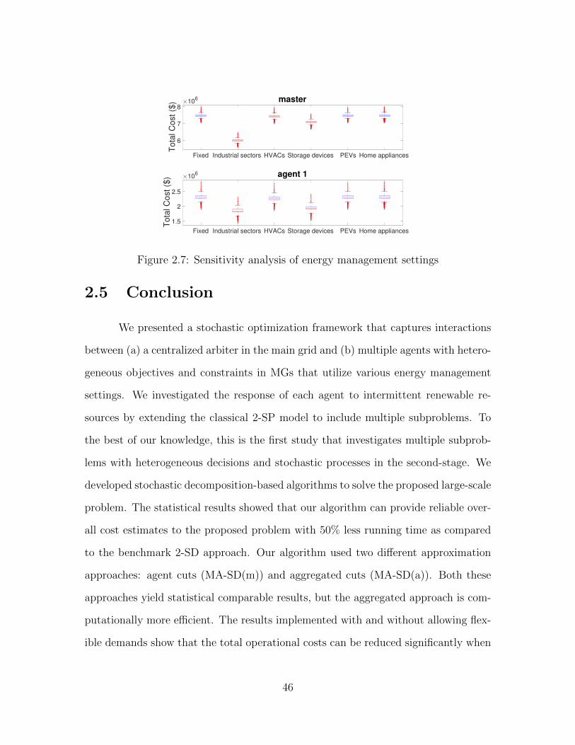
Fixed Industrial sectors HVACs Storage devices PEVs Home appliances

6

7

8

Tota

l C

ost ($

) 106 master

Fixed Industrial sectors HVACs Storage devices PEVs Home appliances

1.5

2

2.5

Tota

l C

ost ($

) 106 agent 1

Figure 2.7: Sensitivity analysis of energy management settings

2.5 Conclusion

We presented a stochastic optimization framework that captures interactions

between (a) a centralized arbiter in the main grid and (b) multiple agents with hetero-

geneous objectives and constraints in MGs that utilize various energy management

settings. We investigated the response of each agent to intermittent renewable re-

sources by extending the classical 2-SP model to include multiple subproblems. To

the best of our knowledge, this is the first study that investigates multiple subprob-

lems with heterogeneous decisions and stochastic processes in the second-stage. We

developed stochastic decomposition-based algorithms to solve the proposed large-scale

problem. The statistical results showed that our algorithm can provide reliable over-

all cost estimates to the proposed problem with 50% less running time as compared

to the benchmark 2-SD approach. Our algorithm used two different approximation

approaches: agent cuts (MA-SD(m)) and aggregated cuts (MA-SD(a)). Both these

approaches yield statistical comparable results, but the aggregated approach is com-

putationally more efficient. The results implemented with and without allowing flex-

ible demands show that the total operational costs can be reduced significantly when

46

customer demand is flexible by effective utilization of the renewable resources. Our

experiments show that cost reductions are more prominent in the main grid than at

individual agents. The sensitivity analysis reveals that the flexibility in the industrial

sector has the potential to contribute the most towards the total cost reduction. The

results also indicate storage devices play a critical role in cost reductions. While the

inclusion of power flow equations increases the computational requirements, they are

necessary to identify system congestion. This is highlighted by the increase in total

cost when flow balance constraints are considered in the proposed MA-SP. Finally,

we studied how the activities of these flexible demands fluctuate with variations of

renewable generations during a day.

The structure of our algorithm involves solving several independent subprob-

lems (corresponding to MGs). This structure is naturally fit for an implementation of

distributed/parallel computing, which will be taken up as part of our future study. In

a smart grid, MGs not only are buyers but also can sell power back to the main grid to

increase utilization of renewable energy over the entire power system. Furthermore,

they are allowed to make transactions with other MGs in the system as well. These

features will also be addressed in our future work.

47

Chapter 3

Stochastic Optimization for

Flow-shop Scheduling with On-site

Renewable Energy Generation

using a case in the United States

S. Wang, S. J. Mason, and H. Gangammanavar, “Stochastic optimization for flow-shop scheduling with on-site renewable energy generation using a case in the UnitedStates,” Computers & Industrial Engineering, Vol. 149, 2020.

Nomenclature

Sets

B set of ESSs; indexed by i = 1, 2, . . . |B|

J set of jobs; indexed by j = 1, 2, . . . |J |

F set of job families; indexed by f, g = 1, 2, . . . |F |

M set of machines; m = 1, 2, . . . |M |

48

R set of renewable generators; r = 1, 2, . . . |R|

T set of time periods; t = 1, 2, . . . |T |

Parameters

wj weight (priority) of job j ∈ J

l length of a time slot [h]

pmj processing time of job j ∈ J on machine m ∈M [h]

sfg setup time between job family f ∈ F and g ∈ F [h]

bmini minimum charging/discharging rate of ESS i ∈ B [kW]

bmaxi maximum charging/discharging rate of ESS i ∈ B [kW]

Emini minimum energy level of ESS i ∈ B [kWh]

Emaxi maximum energy level of ESS i ∈ B [kWh]

qzmf unit power consumed by idling at family f ∈ F on machine m ∈ M

[kW]

qlmfg unit power consumed by a setup between job family f ∈ F and g ∈ F

on machine m ∈M [kW]

cdt unit energy purchasing cost in time period t ∈ T [$/kWh]

cut unit energy selling price in time period t ∈ T [$/kWh]

cEit unit energy storage cost of ESS i ∈ B in time period t ∈ T [$/kWh]

ρt = 1 if the manufacturing plant is allowed to feed power into the electric-

ity grid during time period t ∈ T when the selling price cut ≤ purchasing

price cdt , 0 otherwise

ωrt random variable, power generated by renewable generator r at time

t ∈ T [kW]

Decision Variables

xmjt = 1 if job j ∈ J is started on machine m ∈M at the beginning of time

period t ∈ T ; otherwise = 0

49

ymjt = 1 if job j ∈ J is processed on machine m ∈ M during time period

t ∈ T ; otherwise = 0

zmft = 1 if machine m ∈ M is idle at job family f ∈ F during time period

[t, t+ 1); otherwise = 0

vmfgt = 1 if machine m ∈ M starts to make a setup operation for changing

job family f ∈ F to job family g ∈ F at the beginning of time period

t ∈ T ; otherwise = 0

omfgt = 1 if machine m ∈ M is doing a setup for changing job family f ∈ F

to job family g ∈ F during time period t ∈ T ; otherwise = 0

dt power purchased from the grid in time period t ∈ T [kW]

ut power sold to the grid in time period t ∈ T [kW]

bit ESS charging/discharging rate during time period t ∈ T [kW]. When

bit is positive, the ESS i ∈ B is in charging status; otherwise, it is in

discharging status

Eit Energy state of ESS i ∈ B in time period t ∈ T [kWh]

at underutilized renewable generation in time period t ∈ T [kW]

Acronyms and Abbreviations

GHG greenhouse gas

TOU time-of-use

ECA energy-cost-aware

ESS energy storage system

MILP mixed-integer linear program

ESF extensive scenario formulation

TWCT total weighted completion time

EC energy cost

50

2-SP two-stage stochastic program

SAA sample average approximation

CI confidence interval

3.1 Introduction

Today, protecting the environment is one of the most critical issues faced by

citizens of the world. While, with the development of economic globalization, global

demand for almost any type of product is continuously growing. As a result, the

industrial sector has a high energy demand to satisfy production demand. For exam-

ple, the industrial sector accounted for 32% of total U.S. energy consumption in 2018

[52] according to a report from the U.S. Energy Information Administration. The

main energy sources used by the sector are natural gas, petroleum, electricity, renew-

able sources, and coal. Although the share of renewable sources has been increasing

over the past 60 years, it is still less than 10% of all energy sources. As we know,

non-renewable energy sources can cause environmental issues, especially the emission

of greenhouse gas (GHG). Another U.S. Energy Information Administration report

claims that the industrial sector consumes about 25% of all electricity in use [53]. To

meet excessive peak electricity demands and decrease GHG emissions, load shifting

and utilizing renewable resources are under consideration by Governments, society,

and industry. Load shifting, which is also known as demand response, allows to cur-

tail or shift energy demands in response to economic incentives. In a smart grid,

any kind of end-use customer can gain benefits from adopting a demand response

program. While, industrial sector has the potential to take more advantage of cost

reduction by utilizing demand response [54].

Time-of-use (TOU) electricity pricing schemes vary prices during the day.

51

Higher (lower) costs are charged during peak (off-peak) demand hours. TOU pricing

schemes are used by utilities to motivate manufacturing plants to reduce consump-

tion at peak times by shifting energy use from peak hours to off-peak hours. This

shifting activity, which is referred to as demand response, can increase time-related

scheduling objectives. Energy-cost-aware (ECA) manufacturing is a way to utilize de-

mand response. Its objective is to minimize energy costs at the operational level by

determining optimal job scheduling and/or lot-sizing while considering time-varying

electricity prices [55]. Using on-site electricity generators, some industrial facilities

produce electricity for use. In an ECA manufacturing system, industrial facilities

also can sell some of the electricity that they generate back to the power grid for

compensation.

An effective way to reduce GHG emissions is to utilize environment-friendly re-

newable energy resources, which have received significant research attention in recent

years. Renewable resources are the fastest growing among all energy resources, with

their consumption expected to increase by an average 2.3% per year between 2015

and 2040, according to the U.S. Energy Information Administration [56]. Moreover,

some governments and organizations such as RE100 have committed to encourag-

ing businesses to consider using 100% renewable power. According to its website,

UPS invested $18 million in on-site solar panels, which expanded UPS’s solar power

generating capacity by 10 megawatts in 2017. Further, it is estimated that on-site

wind energy resource development is feasible for about 44% of the continental U.S.’s

buildings, according to a report by the National Renewable Energy Laboratory [57].

Unfortunately, the availability of wind and solar energy, which are two signifi-

cant renewable energy resources, is uncertain, as it fluctuates with weather variations.

Generation can vary at different times over a day and at the same time period over

different days. Properly addressing the uncertainties inherent in renewable energy re-

52

sources can mitigate potential scheduling solution inaccuracies. Further, developing

effective strategies for handling the intermittent nature of renewable energy resources

can improve the effectiveness of renewable energy utilization in production environ-

ments. To mitigate renewable energy availability challenges, energy storage systems

(ESSs) are utilized to store intermittent renewable energy and use it when needed.

To the best of our knowledge, Liu [58] presents the first study that integrates

renewable energy supply into production scheduling while considering the uncertainty

of renewable energy availability using interval number theory. Unfortunately, little

research has been done since that simultaneously considers both ECA production

scheduling and the utilization of uncertain renewable resources for energy genera-

tion. Given this motivation, we study a flow shop scheduling problem with sequence-

dependent setups under a TOU pricing scheme. Power purchased from the main grid,

generated by grid-connected on-site renewable generators such as wind turbines and

solar panels, and discharged from ESSs are available energy sources for the man-

ufacturing process under study. Energy consumption is machine status-related, as

job processing, production setups, and machine idling consume different amounts of

energy.

Figure 3.1 describes the methodological approaches used in this research. We

first formulate a two-stage, bi-objective stochastic ECA problem. Then the problem

is solved through a ε-constraint framework with L-shaped method. Finally, experi-

ments were conducted to illustrate the performance of our proposed algorithm and

its effectiveness in realizing energy-related objectives in manufacturing. The main

contributions of this research are threefold: (1) we study an ECA problem that in-

tegrates an energy procurement problem with a flow shop scheduling problem to

minimize total weighted completion time and energy costs simultaneously by deter-

mining optimal job schedules and energy supply decisions; (2) we develop a two-stage,

53

Model

Formulate a bi-objective stochastic

ECA problem

Re-write theproblem as a bi-objective 2-SP

Algorithm

Convert the probleminto a single

objective 2-SP bytransforming oneobjective into an 𝜖-

constraint

Solve the 2-SPusingL-shaped method

Obtain Paretooptimal solutions

Experiment

Investigate theperformance of the

𝜖-constraintframework

Study the effect ofsetup costs

Study the impact ofintegrating on-siterenewable energy on

the productionschedules and energy

costs

Study the impact ofdifferent sources ofrenewable energy on

the productionschedules and energy

costs

Figure 3.1: Flow chart of methodological approaches performed in this research

multi-objective stochastic problem for the ECA problem. In the first stage, we pro-

pose a time-indexed, mixed-integer linear program (MILP) which captures several

practical features of the flow shop scheduling problem. The second stage determines

the energy transactions between the manufacturing plant and the power grid in the

context of uncertain renewable energy and ESSs under a TOU pricing scheme; (3)

we conduct a case study to investigate the performance of our algorithm, the effects

of setups on energy cost, and demonstrate the potential benefits of utilizing on-site

renewable resources and ESSs.

54

The rest of the paper is organized as follows. After the current literature is

reviewed in Section 3.2, our mathematical model is presented in Section 3.3. Then,

two-stage, multi-objective decomposition algorithms are implemented in Section 3.4,

followed by a discussion of our computational experiments in Section 3.5 Finally, we

offer conclusions and future research directions in Section 3.6.

3.2 Literature Review

As many areas of the world are facing environmental issues surrounding the

consumption of fossil fuels and concomitant GHG emissions, efforts to make produc-

tion scheduling sustainable have become a key focus for many companies. Lots of

literature on energy-aware production scheduling has evolved in recent years. Giret

et al. [59], Biel and Glock [60], and Gahm et al. [61] present a comprehensive review

of this research stream. Giret et al. [59] review the existing literature on sustainable

scheduling and focus on environmental and economic development. Biel and Glock

[60] provide a survey on decision support models for energy-efficient production plan-

ning. Gahm et al. [61] develop a framework for energy-efficient scheduling and classify

the literature into three aspects–energetic coverage, energy supply, and energy de-

mand. Gahm et al. [61] state that machine processing states and job-related features

both impact energy consumption during production operations, non-processing states

such as machine idling, system on/off, and setups can also affect energy consumption

requirements.

Yildirim and Mouzon [62] propose a multi-objective framework for a single

machine scheduling problem to minimize both energy consumption and job comple-

tion time by turning off the machine instead of leaving it idle when not in use. Liu

et al. [63] study a flow shop scheduling problem with state-dependent setup times

55

to minimize energy consumption and tardiness penalties. After introducing fuzzy set

theory to describe the uncertainty of processing time and due dates, an improved

hybrid genetic algorithm is developed for solving the problem.

Luo et al. [64] investigate a hybrid flow shop scheduling problem under a four-

period TOU pricing scheme to minimize makespan and power consumption. Their

experimental results show that increasing the length of each TOU period can reduce

electricity costs without affecting makespan. Similarly, under a TOU tariff, Ding

et al. [65] propose a time-interval-based mixed-integer, linear model and a column

generation heuristic for a parallel machine scheduling problem to minimize electricity

costs while keeping the makespan within a given production deadline. Understanding

the tradeoff between electricity costs and makespan can provide insights for manage-

ment to help determine the maximum acceptable production time under TOU pricing

schemes.

Moon and Park [66] investigate production scheduling problems integrated

with on-site renewable generation, fuel cells, and ESSs. They propose a model with

two subproblems for a flexible job shop to minimize the sum of makespan-related

production costs, the cost of purchasing power from the grid, the cost of distributed

generations, and the cost of an ESS under a TOU pricing scheme. The first sub-

problem is a production scheduling problem with a given energy schedule, while the

second subproblem is an energy scheduling problem for a given flexible job shop. By

solving these two subproblems alternately and repeatedly, a near-optimal solution is

found. In their model, Moon and Park [66] assume that the minimum and maximum

amounts of renewable energy available for each time period within the planning hori-

zon are known in advance. Then the amount of energy generated for a given time

period is determined by the model. Zhai et al. [67], who study a flow shop scheduling

problem in the context of a real-time pricing scheme, also consider on-site renewable

56

generation. Time series models are used to forecast hourly wind speeds and elec-

tricity prices, which increase data accuracy as compared to using the fixed intervals

adopted by Moon and Park [66]. After obtaining forecast data, hourly wind speeds

and electricity prices are fed into a manufacturing scheduling model to minimize

energy costs. Unfortunately, this procedure requires that all data is predetermined

without any consideration of uncertainty. Similarly, Zhang et al. [68] investigate the

effect of on-site photovoltaic and ESSs on a flow shop under a TOU pricing scheme.

However, the uncertainty of solar generation is not considered in the study.

Liu [58] presents a mathematical model for a single-machine scheduling prob-

lem integrated with renewable generation and an ESS. Liu [58] represents the uncer-

tainty of renewable energy resources by using interval number theory. The energy

generated by renewable energy resources during each time period is bounded by an

interval and the interval boundaries are randomly generated from a uniform distri-

bution. The author assumes that the plant will purchase any power needed from

the main grid if the renewable energy stored in batteries runs out in any time pe-

riod. Two models are considered: 1) simultaneously minimizing total weighted flow

time and GHG emissions using a lexicographic-weighted Tchebycheff method and 2)

minimizing total weighted flow time by considering a GHG emission constraint.

Biel et al. [69] propose a two-stage stochastic optimization procedure for a

flow shop scheduling problem with on-site wind power under a TOU pricing scheme

to minimize total weighted flow time and energy costs. In the first stage, a bi-objective

MILP is used to evaluate a number of generated wind power scenarios which form

an extensive scenario formulation (ESF). A weighted sum algorithm is used to tackle

multiple objective functions. Then, based on real-time wind power data, energy

supply decisions are adjusted in the second stage. Fazli Khalaf and Wang [70] propose

a two-stage stochastic MILP for a flow shop problem with on-site renewable resources

57

and ESS under day-ahead and real-time electricity pricing schemes. The first stage

determines job schedules and minimizes energy purchase cost procured from the day-

ahead plan by considering forecasted renewable energy generation, while the second

stage compensates for the mismatch between forecasted and actual renewable energy

and minimizes energy costs under a real-time pricing scheme.

As Table 3.1 shown, only a few research studies have considered ECA produc-

tion scheduling with stochastic renewable energy sources simultaneously. Further,

sequence-dependent setups, which occur when production switches between different

job families Wang et al. [71], have been ignored in the literature. These setups not

only affect time-related objectives but also affect energy costs and demand require-

ments [72]. Motivated by these gaps in the literature, the main goal of our study is

to examine these important topics.

3.3 Problem Formulation

Consider a flow shop comprised of |M | production machines. A set of jobs J

of varying weights (priorities) wj is released at the beginning of the time horizon of

interest. Each job j ∈ J must be processed with processing time pmj on each machine

m ∈ M sequentially. A sequence-dependent setup time is required for changeovers

when the job family changes from f ∈ F to g ∈ F \ f on any machine. Different

machine statuses (i.e., job processing, setup, and idling) consume different amounts of

energy. The energy required for operating machines can be purchased from the main

power grid, generated by on-site renewable generators, and/or discharged from ESSs.

On-site renewable generation can be used to run production, charge ESSs, and/or

be sold to the main grid for compensation (Figure 3.2). In our study, electricity

prices are governed by a TOU pricing scheme containing three different electricity

58

Tab

le3.

1:Sum

mar

yof

revie

wed

EC

Apro

duct

ion

sched

uling

pro

ble

ms

Stu

dy

Mac

hin

een

vir

onm

ent

Mac

hin

eSta

tus

RE

SSto

chas

tic

ESS

Yildir

iman

dM

ouzo

n(2

012)

Sin

gle

mac

hin

eP

roce

ssin

g,id

ling,

and

ON

/OF

F-

--

Liu

etal

.(2

017)

Flo

wsh

opP

roce

ssin

g,id

ling,

stat

e-dep

enden

tse

tup,

and

ON

/OF

F-

--

Luo

etal

.(2

013)

Hybri

dflow

shop

Pro

cess

ing

and

idling

--

-D

ing

etal

.(2

016)

Par

alle

lm

achin

eP

roce

ssin

g-

--

Moon

and

Par

k(2

014)

Fle

xib

lejo

bsh

opP

roce

ssin

gan

did

ling

(no

cost

)Y

esN

oY

es

Zhai

etal

.(2

017)

Flo

wsh

opP

roce

ssin

g,id

ling,

and

ON

/OF

FW

ind

No

-

Zhan

get

al.,

(201

7)H

ybri

dflow

shop

Pro

cess

ing

Sol

arN

oY

esL

iu(2

016)

Sin

gle

mac

hin

eP

roce

ssin

gY

esY

esY

esB

iel

etal

.(2

018)

Flo

wsh

opP

roce

ssin

gW

ind

Yes

-F

azli

Khal

afan

dW

ang

(201

8)F

low

shop

Pro

cess

ing

Win

d&

Sol

arY

esY

es

59

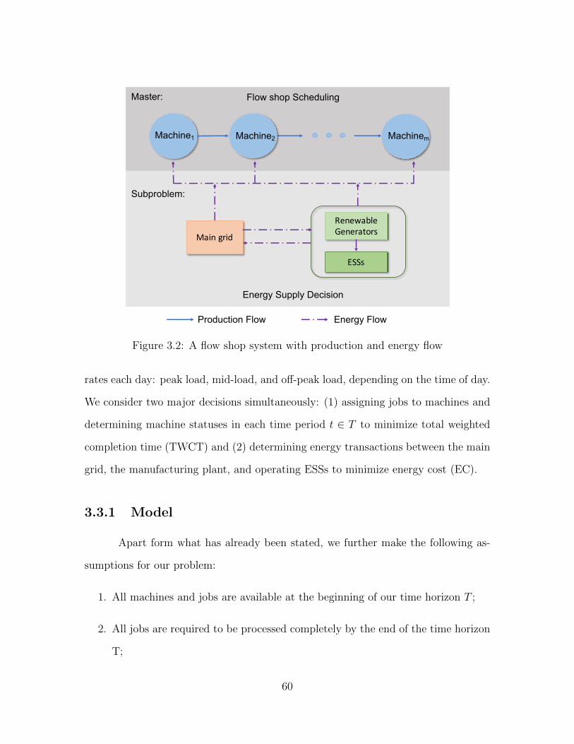
Main grid

RenewableGenerators

ESSs

Master:

Subproblem:

Flow shop Scheduling

Energy Supply Decision

Production Flow Energy Flow

Machine1 Machine2 Machinem

Figure 3.2: A flow shop system with production and energy flow

rates each day: peak load, mid-load, and off-peak load, depending on the time of day.

We consider two major decisions simultaneously: (1) assigning jobs to machines and

determining machine statuses in each time period t ∈ T to minimize total weighted

completion time (TWCT) and (2) determining energy transactions between the main

grid, the manufacturing plant, and operating ESSs to minimize energy cost (EC).

3.3.1 Model

Apart form what has already been stated, we further make the following as-

sumptions for our problem:

1. All machines and jobs are available at the beginning of our time horizon T ;

2. All jobs are required to be processed completely by the end of the time horizon

T;

60

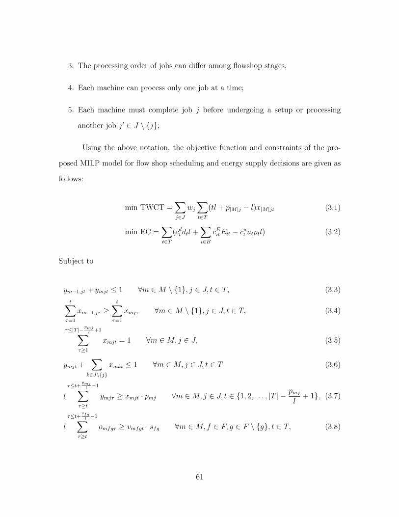
3. The processing order of jobs can differ among flowshop stages;

4. Each machine can process only one job at a time;

5. Each machine must complete job j before undergoing a setup or processing

another job j′ ∈ J \ j;

Using the above notation, the objective function and constraints of the pro-

posed MILP model for flow shop scheduling and energy supply decisions are given as

follows:

min TWCT =∑j∈J

wj∑t∈T

(tl + p|M |j − l)x|M |jt (3.1)

min EC =∑t∈T

(cdtdtl +∑i∈B

cEitEit − cut utρtl) (3.2)

Subject to

ym−1,jt + ymjt ≤ 1 ∀m ∈M \ 1, j ∈ J, t ∈ T, (3.3)

t∑τ=1

xm−1,jτ ≥t∑

τ=1

xmjτ ∀m ∈M \ 1, j ∈ J, t ∈ T, (3.4)

τ≤|T |−pmjl

+1∑τ≥1

xmjt = 1 ∀m ∈M, j ∈ J, (3.5)

ymjt +∑

k∈J\j

xmkt ≤ 1 ∀m ∈M, j ∈ J, t ∈ T (3.6)

l

τ≤t+pmjl−1∑

τ≥t

ymjτ ≥ xmjt · pmj ∀m ∈M, j ∈ J, t ∈ 1, 2, . . . , |T | − pmjl

+ 1, (3.7)

l

τ≤t+sfgl−1∑

τ≥t

omfgτ ≥ vmfgt · sfg ∀m ∈M, f ∈ F, g ∈ F \ g, t ∈ T, (3.8)

61

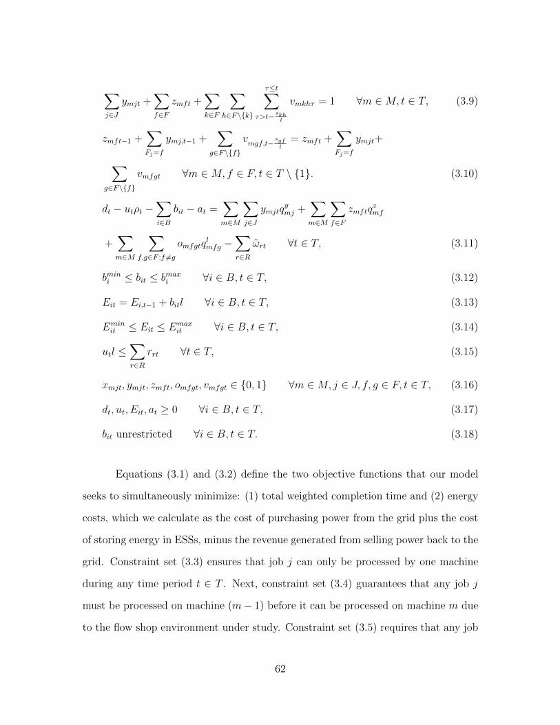
∑j∈J

ymjt +∑f∈F

zmft +∑k∈F

∑h∈F\k

τ≤t∑τ>t− skh

l

vmkhτ = 1 ∀m ∈M, t ∈ T, (3.9)

zmft−1 +∑Fj=f

ymj,t−1 +∑

g∈F\f

vmgf,t−

sgfl

= zmft +∑Fj=f

ymjt+

∑g∈F\f

vmfgt ∀m ∈M, f ∈ F, t ∈ T \ 1. (3.10)

dt − utρt −∑i∈B

bit − at =∑m∈M

∑j∈J

ymjtqymj +

∑m∈M

∑f∈F

zmftqzmf

+∑m∈M

∑f,g∈F :f 6=g

omfgtqlmfg −

∑r∈R

ωrt ∀t ∈ T, (3.11)

bmini ≤ bit ≤ bmaxi ∀i ∈ B, t ∈ T, (3.12)

Eit = Ei,t−1 + bitl ∀i ∈ B, t ∈ T, (3.13)

Eminit ≤ Eit ≤ Emax

it ∀i ∈ B, t ∈ T, (3.14)

utl ≤∑r∈R

rrt ∀t ∈ T, (3.15)

xmjt, ymjt, zmft, omfgt, vmfgt ∈ 0, 1 ∀m ∈M, j ∈ J, f, g ∈ F, t ∈ T, (3.16)

dt, ut, Eit, at ≥ 0 ∀i ∈ B, t ∈ T, (3.17)

bit unrestricted ∀i ∈ B, t ∈ T. (3.18)

Equations (3.1) and (3.2) define the two objective functions that our model

seeks to simultaneously minimize: (1) total weighted completion time and (2) energy

costs, which we calculate as the cost of purchasing power from the grid plus the cost

of storing energy in ESSs, minus the revenue generated from selling power back to the

grid. Constraint set (3.3) ensures that job j can only be processed by one machine

during any time period t ∈ T . Next, constraint set (3.4) guarantees that any job j

must be processed on machine (m− 1) before it can be processed on machine m due

to the flow shop environment under study. Constraint set (3.5) requires that any job

62

j can only be processed by each machine m once. Next, constraint set (3.6) ensures

that any machine m can process job j only after job j is assigned to the machine. Any

machine m cannot be interrupted once it starts processing a job, which is guaranteed

by constraint set (3.7). Similarly, constraint set (3.8) ensures that a setup operation

on machine m cannot be interrupted once it starts.

The constraints for representing the three machine states of interest are in-

spired by [73]. Constraint set (3.9) ensures that any machine can only be in exactly

one state, job processing, setup, or idling, in each time period t ∈ T . Further, any

change of machine state induces a setup operation (3.10). The power needed for

running the flow shop’s machines includes power purchased from the grid, power dis-

charged from ESSs, and power generated by on-site renewable generators. Constraint

set (3.11) is a power balance equation which specifies that the total available power

should meet the total power demand at every time period. In (3.11), bit is the charg-

ing/discharging rate of ESS i ∈ B during time period t ∈ T . The value of bit will be

positive if the ESS i ∈ B is charging; otherwise, it is in a discharging mode. These de-

cisions are bounded by the charging/discharging rates of the ESS (3.12). Constraint

set (3.13) is the system dynamics equations which specify the state of ESS i ∈ B (see

[54] for details). In (3.13), the initial state Ei0 is assumed to be given. Constraint

set (3.14) ensures that the state of ESS i ∈ B is always between its lower and upper

bounds. The quantity of renewable generation determines the upper bound of the

power sold to the main grid (3.15). Finally, constraint sets (3.16) - (3.18) provide

variable types and limits on the decision variables in our model.

63

3.3.2 Formulation of the Two-stage Stochastic Programming

Model

The proposed scheduling and energy supply problem can be written as a two-

stage stochastic program (2-SP) to model the stochastic nature of on-site renewable

energy resources. Since scheduling decisions are made prior to the realization of re-

newable energy availability, they are non-anticipative in nature [1]. We succinctly use

a single decision vector x ∈ X to collectively denote scheduling variables xmjt, ymjt,

zmft, omfgt and vmfgt, where X denotes the feasible set. Once scheduling decisions

are made, energy supply requirements are informed by this decision vector and the

realization of renewable generation ω of its stochastic process ω. This allows us to

write the entire model as:

min∑j∈J

wj∑t∈T

(tl + p|M |j − l)x|M |jt + Eh(x, ω) (3.19a)

s.t. (3.3) – (3.10) and (3.16),

where the recourse function h(x, ω) is given by:

h(x, ω) = min∑t∈T

(cdtdt − cut ut +∑i∈B

cEitEit) (3.19b)

s.t. (3.11) – (3.15), (3.17), and (3.18).

According to the general formulation of a stochastic problem [1], problem (3.19a)

is commonly referred to as the master problem, while problem (3.19b) is known as

the subproblem. Note that the decision variables in the master problem (3.19a) are

binary variables, while the decision variables in subproblem (3.19b) are continuous.

While first-stage decisions affect the right-hand side of equation (3.11) (renewable

64

generation), the recourse matrix characterized by the left-hand side in equation (3.11)

and the transfer matrix characterized by the right-hand side of equation (3.11) are

independent of uncertainty. Therefore, the above formulation is a 2-SP with fixed

recourse [1].

3.4 Two-Stage, Multi-Objective Stochastic Solu-

tion Scheme

Our problem is a bi-objective problem whose solution is described by a Pareto-

optimal set, rather than a unique solution. In general, the resolution of multi-objective

stochastic problems involves two kinds of transformations: transforming the multi-

objective problem into a single-objective problem and converting the stochastic prob-

lem into its equivalent deterministic problem [74, 75]. Caballero et al. [76] classify the

existing techniques for the solution of multi-objective stochastic problems according to

the order in which transformations are carried out. The multi-objective approach first

transforms the stochastic multi-objective problem into its equivalent multi-objective,

deterministic problem. Alternatively, the stochastic approach transforms the stochas-

tic multi-objective problem into a single-objective stochastic problem in the first step.

Multi-objective stochastic optimization approaches have been studied in vari-

ous fields. Tricoire et al. [77] formulate a bi-objective stochastic covering tour problem

using a sample average approximation (SAA) technique, which is then solved by a

branch-and-cut method within an ε-constraint algorithm. Osorio et al. [78] pro-

vide an approach which combines the SAA method and the augmented ε-constraint

algorithm. Biel et al. [69] propose a two-stage stochastic optimization framework

for flow shop scheduling problems with on-site wind power. In the first stage, a

65

bi-objective MILP is formulated via an ESF considering all generated wind power

scenarios simultaneously. The bi-objective objective function is transformed into a

single objective using a weighted sum approach. In the second stage, energy supply

decisions are adjusted according to the realization of actual wind power. Compared to

the ε-constraint algorithm, weighted sum approach has two main drawbacks [77]: (1)

it is difficult for decision-makers to define weights for conflicting objectives a priori;

and (2) it can only find supported solutions and missing other attractive candidates.

So motivated by [79], our solution approach for solving the bi-objective stochastic

problem adopts an ε-constraint framework to transform the multi-objective problem

into a problem with only one objective. The L-shaped method is used to tackle the

2-SP. The details of ε-constraint framework and the L-shaped method described in

the following subsections.

3.4.1 ε-constraint Framework

The ε-constraint algorithm [80] consists of transforming a multi-objective prob-

lem into a single objective problem. To do this, decision-makers must select one

objective function to remain as the objective function and transform all others into

constraints bounded by a set of parameters ε. These additional constraints are named

as ε-constraints.

To enumerate all Pareto optimal solutions, the algorithm iteratively solves

single-objective optimization problems for each value of the ε parameters. The for-

mulation introduced in Section 3.3 has two objective functions: TWCT and EC. The

discrete-time periods result in integer values of TWCT. If we convert TWCT into

an ε-constraint, it is easy to change the value of parameter ε by one unit from one

iteration to the next [79]. Therefore, for computational convenience, we choose EC

66

as the main objective function and TWCT is transformed into an ε-constraint. By

introducing these changes, the master problem (3.19a) can be reformulated as:

min Eh(x, ω) (3.20)

s.t.∑j∈J

wj∑t∈T

(tl + p|M |j − l)x|M |jt ≤ ε

(3.3) – (3.10), (3.16).

Note that the two-stage stochastic programming framework in problem (3.20) is main-

tained by converting TWCT to an ε-constraint.

Figure 3.3 shows a flow chart for the two decomposition algorithms integrated

with the ε-constraint framework [79]. Given the negative correlation between our two

objective functions (i.e., TWCT increases as EC decreases), the maximum (minimum)

value of TWCT, which is denoted as b (a), is obtained when EC reaches its smallest

(largest) value. Let V denote a set of paired objective functions EC and TWCT. We

begin our algorithm by setting the value of parameter ε = b. The ε value is decreased

by one unit (δ) in each iteration. We call this an ε-iteration within which one pair

of optimal solutions is obtained using our decomposition algorithms. Note that ε is

an upper bound of TWCT, not the value of TWCT. The actual TWCT value can be

calculated using the ε-constraint during each ε-iteration. The ε-iteration stops when

ε = a. Finally, the Pareto front is identified from the set V .

3.4.2 L-shaped Method

Classical 2-SPs are well studied in the literature and several algorithms have

been proposed to analyze these problems. To achieve computational tractability,

many of these methods represent uncertainty through a finite number of realizations

67

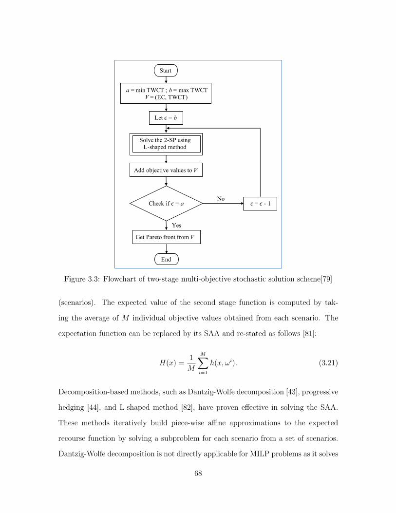
a = min TWCT ; b = max TWCTV = (EC, TWCT)

Let 𝜖 = b

Solve the 2-SP usingL-shaped method

Check if 𝜖 = a

Get Pareto front from V

Add objective values to V

Start

End

𝜖 = 𝜖 - 1No

Yes

Figure 3.3: Flowchart of two-stage multi-objective stochastic solution scheme[79]

(scenarios). The expected value of the second stage function is computed by tak-

ing the average of M individual objective values obtained from each scenario. The

expectation function can be replaced by its SAA and re-stated as follows [81]:

H(x) =1

M

M∑i=1

h(x, ωi). (3.21)

Decomposition-based methods, such as Dantzig-Wolfe decomposition [43], progressive

hedging [44], and L-shaped method [82], have proven effective in solving the SAA.

These methods iteratively build piece-wise affine approximations to the expected

recourse function by solving a subproblem for each scenario from a set of scenarios.

Dantzig-Wolfe decomposition is not directly applicable for MILP problems as it solves

68

the dual of the master problem. Progressive hedging, which is a scenario-based de-

composition method, requires selecting an appropriate proximal parameter which is

instance-dependent and hard to determine. We base our solution approach on the

L-shaped method.

To simplify our exposition of L-shaped method, we use a succinct representa-

tion of the 2-SP model [1]:

min c>x+ Eh(x, ω) (3.22a)

s.t. x ⊂ Zn1 × Rn2 ,

where

h(x, ω) = min d>y (3.22b)

s.t. Wy ≤ r(ωn)− T (ω)x,

y ≥ 0.

Auxiliary variable η is used to represent the approximation of the expected recourse

function Eh(x, ω). At the beginning of the algorithm, the value of η is set as

−∞ or an appropriate approximation value. The algorithm begins with the original

constraints only, X 0 := x, η|Ax = b ⊂ Z+ × R+. In iteration k, the algorithm first

solves the MILP

minc>x+ η|(x, η) ∈ X k, (3.23)

to obtain the solution xk. Then, with this solution and a realization ωi ∈ Ω, the opti-

mal dual solution πk is identified by solving the subproblem h(xk, ωi). This procedure

is enumerated for every realization ωi ∈ Ω. Using these dual solutions, we obtain a

69

lower bounding optimality cut as follows:

lk(x, η) :=∑i∈S

piπ>i [r(ωi − T (ωi)xk)]− η ≤ 0, (3.24)

where pi is the probability of scenario ωi and S is the number of scenarios. Then, the

feasible region is updated as:

X k+1(x) = X k(x) ∩ (lk(x, η) ≤ 0). (3.25)

Note that our subproblem (3.19b) satisfies the relative complete recourse property

which means our subproblem has feasible solutions for all ωi ∈ Ω and x ∈ X 0.

Therefore, we omit feasibility cuts here. For more details, we refer the reader to [1].

3.5 Computational Experiments

We consider a three-machine flow shop in which three jobs need to be processed

within the planning horizon (T = 24 hours). The length of each time slot is one hour

and 10 random problem instances are created. The data for weights of the jobs

(wj), job processing times (pmj), and the processing power requirements of machines

(qymj) are from [69]. Setup times (sfg) and the power consumed during setup (qlmfg)

are randomly generated from uniform distributions [1 h, 3 h] and [1 kW, 15 kW],

respectively.

One energy storage system is installed and available near the plant. Renewable

generation data was extracted from the Western Wind and Solar Integration Study

[49]. An experiment utilizes solar generation if no specific details are given. To

reduce the impact of seasonal variations, we only adopt the renewable generation

data from spring. The number of scenarios considered in building our instances is

70

1000. Electricity prices follow a day-ahead TOU pricing scheme (Figure 3.4) which

is derived from a rate schedule for industrial customers of California’s Pacific Gas

and Electric Company [83]. The feed-in electricity price is set to 0.08923 USD/kWh

as found in the Electric-Renewable Market Adjusting Tariff of the Pacific Gas and

Electric Company [84].

ElectricityPrice($/kWh)

0

0.02

0.04

0.06

0.08

0.1

0.12

0.14

0.16

1 2 3 4 5 6 7 8 9 10 11 12 13 14 15 16 17 18 19 20 21 22 23 24

Time

0.0821

0.10981

0.15018

0.10981

0.0821

Figure 3.4: TOU Pricing Scheme

Our L-shaped method-based ε-constraint algorithm was implemented in C

on a MacBook Pro running an Intel Core i7 CPU@3.3GHz (Dual-Core) with 16 GB

Memory @2133 MHz. All MILPs were solved using CPLEX 12.7 callable subroutines.

During each ε-iteration, we begin by using an optimization process to identify

the optimal solution for the master problem and the corresponding prediction value.

Then, a verification phase is applied, where the solution of the master problem is

fixed, and the subproblem is simulated using independent and identically distributed

observations. Using the objective values, a confidence interval (CI) of the upper

bound estimate is built for the expected recourse function.

We begin by illustrating how the ε-constraint framework works using instance

3 (”Ins3s”). The input ε value, corresponding TWCT, and predicted EC are summa-

71

rized in Table 3.2. As mentioned in Section 3.4.1, the actual TWCT is not necessarily

equal to the input ε, which is shown in the results in the 2nd, 5th, and 8th columns

in Table 3.2. For example, when ε is equal to 138, the actual TWCT is 135. Another

feature that should be noted is that TWCT is 135 whenever the input ε is set to 138

or 135. The predicted EC obtained when ε is set to 138 is smaller than the value

obtained when ε is changed to 135. Therefore, (TWCT = 138, EC = 233.737) is

Pareto optimal as (TWCT = 138, EC = 233.737) dominates (TWCT = 135, EC =

234.104), although this Pareto point is obtained when the input ε is 138 not 135.

We say a point (TWCT, EC) dominates another point (TWCT’, EC’) when TWCT’

≥ TWCT and EC ≤ EC’. Therefore, seven Pareto optimal solutions are found for

instance 3, marked by “*” in Table 3.2. Figure 3.5 presents the Pareto frontier of the

ten instances. As we expected, there is a trade-off between TWCT and the predicted

objective value EC: as the TWCT decreases, the predicted EC increases.

Next, we continue to use instance 3 to study the effect of setup costs in our

scheduling problem with both time and energy cost considerations. We create another

problem using Ins3s without considering setup costs, Ins3. Ins3 also contains seven

Pareto optimal solutions which obtain the same TWCT as Ins3s. Figure 3.6 presents

Table 3.2: Input ε, corresponding TWCT, and predicted EC of Ins3s

εTWCT

(hr)Predicted

EC ($)ε

TWCT(hr)

PredictedEC ($)

εTWCT

(hr)Predicted

EC ($)∗138 135 233.737 130 129 240.391 122 120 253.878137 135 234.104 ∗129 129 240.391 121 120 253.878136 135 234.104 128 126 245.790 ∗120 120 253.878135 135 234.104 127 126 245.790 119 117 257.558134 132 234.988 ∗126 126 245.790 118 117 257.558133 132 234.988 125 123 250.909 ∗117 117 257.558∗132 132 234.988 124 123 250.909131 129 240.391 ∗123 123 250.909

*Pareto optimal solution

72

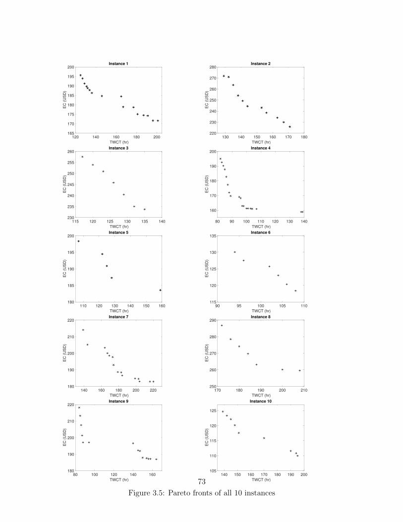
120 140 160 180 200

TWCT (hr)

165

170

175

180

185

190

195

200E

C (

US

D)

Instance 1

130 140 150 160 170 180

TWCT (hr)

220

230

240

250

260

270

280

EC

(U

SD

)

Instance 2

115 120 125 130 135 140

TWCT (hr)

230

235

240

245

250

255

260

EC

(U

SD

)

Instance 3

80 90 100 110 120 130 140

TWCT (hr)

160

170

180

190

200

EC

(U

SD

)

Instance 4

110 120 130 140 150 160

TWCT (hr)

180

185

190

195

200

EC

(U

SD

)

Instance 5

90 95 100 105 110

TWCT (hr)

115

120

125

130

135

EC

(U

SD

)

Instance 6

140 160 180 200 220

TWCT (hr)

180

190

200

210

220

EC

(U

SD

)

Instance 7

170 180 190 200 210

TWCT (hr)

250

260

270

280

290

EC

(U

SD

)

Instance 8

80 100 120 140 160

TWCT (hr)

180

190

200

210

220

EC

(U

SD

)

Instance 9

140 150 160 170 180 190 200

TWCT (hr)

105

110

115

120

125

EC

(U

SD

)

Instance 10

Figure 3.5: Pareto fronts of all 10 instances

73

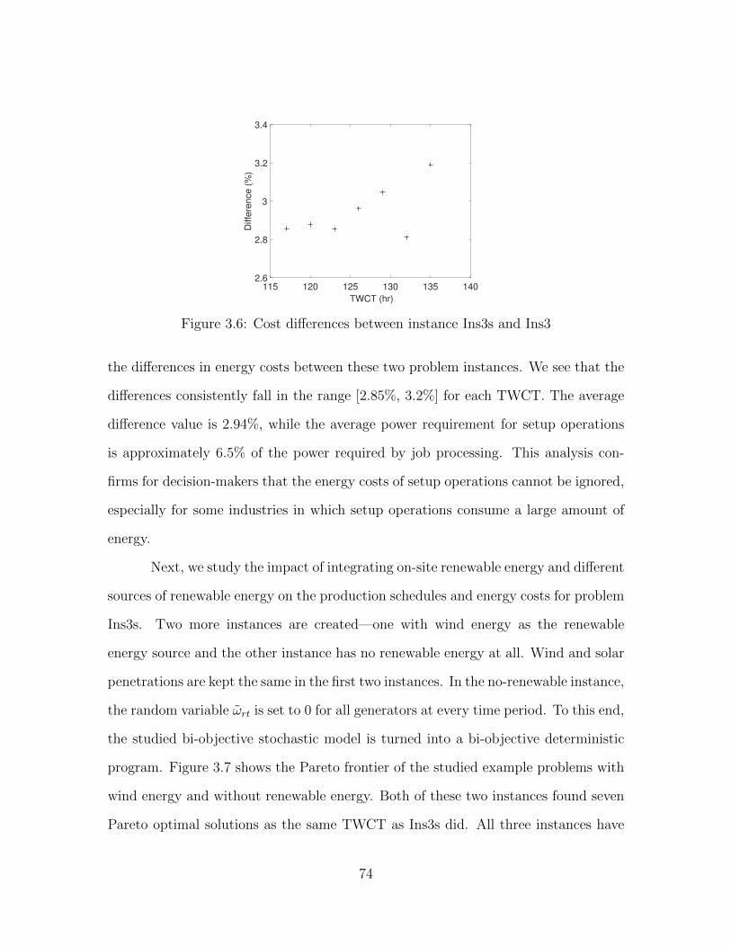
115 120 125 130 135 140

TWCT (hr)

2.6

2.8

3

3.2

3.4

Diffe

ren

ce

(%

)

Figure 3.6: Cost differences between instance Ins3s and Ins3

the differences in energy costs between these two problem instances. We see that the

differences consistently fall in the range [2.85%, 3.2%] for each TWCT. The average

difference value is 2.94%, while the average power requirement for setup operations

is approximately 6.5% of the power required by job processing. This analysis con-

firms for decision-makers that the energy costs of setup operations cannot be ignored,

especially for some industries in which setup operations consume a large amount of

energy.

Next, we study the impact of integrating on-site renewable energy and different

sources of renewable energy on the production schedules and energy costs for problem

Ins3s. Two more instances are created—one with wind energy as the renewable

energy source and the other instance has no renewable energy at all. Wind and solar

penetrations are kept the same in the first two instances. In the no-renewable instance,

the random variable ωrt is set to 0 for all generators at every time period. To this end,

the studied bi-objective stochastic model is turned into a bi-objective deterministic

program. Figure 3.7 shows the Pareto frontier of the studied example problems with

wind energy and without renewable energy. Both of these two instances found seven

Pareto optimal solutions as the same TWCT as Ins3s did. All three instances have

74

115 120 125 130 135

TWCT (hr)

280

300

320

340

360

380

400

420

EC

(U

SD

)

Wind Energy

No Renewable Energy

Figure 3.7: Pareto front for instance 3 with wind energy and without renewable energy

the same trend of reducing EC when increasing TWCT.

During the verification phase, 100 samples are used for different ε parameters

to evaluate the solution. Figure 3.8 presents the energy costs observed at every

TWCT of all three problem instances during the verification phase. It clearly shows

that incorporating renewable energy helps to reduce energy costs for production. On

average, using solar energy and wind energy saves 35.8% and 15.9% over no renewable

generation utilized, respectively. Another observation from Figure 3.8 is that cost

reduction is more prominent when utilizing solar energy than with wind energy as the

average savings is 23.6%. This decrease can be attributed to the different distributions

of solar and wind generation within the time horizon of interest (Figure 3.9). Wind

power distributes evenly during the entire time horizon (Figure 3.9b), while solar

provides more generation during the day time when electricity prices are high (Figure

3.4). Therefore, solar energy can satisfy some or all power demand during these

high electricity price periods. Moreover, surplus solar energy can be stored in energy

storage devices for future use or fed back into the main grid for compensation.

To further study the impact of on-site renewable energy on production sched-

ules and energy costs, we use the optimal first-stage solution as an input to the

75

117 120 123 126 129 132 135

TWCT (hr)

200

220

240

260

280

300

320

340

360

380

400E

C (

US

D)

(a) Objective values of instance 3 with solarenergy

117 120 123 126 129 132 135

TWCT (hr)

200

220

240

260

280

300

320

340

360

380

400

EC

(U

SD

)

(b) Objective values of instance 3 with windenergy

117 120 123 126 129 132 135

TWCT (hr)

200

220

240

260

280

300

320

340

360

380

400

EC

(U

SD

)

(c) Objective values of instance 3 without re-newable energy

Figure 3.8: Objective values of instance 3

5 10 15 20

TWCT

0

50

100

150

200

250

Sola

r genera

tion (

kW

)

(a) Distribution of solar generation

5 10 15 20

TWCT

0

50

100

150

200

250

300

Win

d g

enera

tion (

kW

)

(b) Distribution of wind generation

Figure 3.9: Distributions of solar and wind generation

subproblem. The decision process of the subproblem is simulated by solving an op-

timization problem using independent Monte Carlo samples. Figure 3.10 shows the

results with and without solar energy when TWCT = 132. Production processes,

76

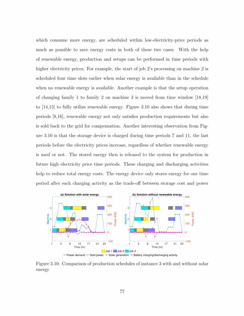
which consume more energy, are scheduled within low-electricity-price periods as

much as possible to save energy costs in both of these two cases. With the help

of renewable energy, production and setups can be performed in time periods with

higher electricity prices. For example, the start of job 2’s processing on machine 2 is

scheduled four time slots earlier when solar energy is available than in the schedule

when no renewable energy is available. Another example is that the setup operation

of changing family 1 to family 2 on machine 3 is moved from time window [18,19]

to [14,15] to fully utilize renewable energy. Figure 3.10 also shows that during time

periods [8,16], renewable energy not only satisfies production requirements but also

is sold back to the grid for compensation. Another interesting observation from Fig-

ure 3.10 is that the storage device is charged during time periods 7 and 11, the last

periods before the electricity prices increase, regardless of whether renewable energy

is used or not. The stored energy then is released to the system for production in

future high electricity price time periods. These charging and discharging activities

help to reduce total energy costs. The energy device only stores energy for one time

period after each charging activity as the trade-off between storage cost and power

1 5 9 13 17 21 24Time (hr)

1

2

3

Machin

e

-100

0

100

200

300

400

Pow

er

(kW

)

(a) Solution with solar energy

Job 1 Job 2 Job 3

1 5 9 13 17 21 24Time (hr)

1

2

3

Machin

e

-100

0

100

200

300

400

Pow

er

(kW

)(b) Solution without renewable energy

Power demand Sold power Solar generation Battery charging/discharging activity

Figure 3.10: Comparison of production schedules of instance 3 with and without solarenergy

77

purchasing cost determines the length of storage periods.

3.6 Conclusions and Future Research

In this paper, we study a flow shop scheduling problem with sequence-dependent

setups, on-site renewable generation, and an available energy storage system. The

model is formulated as a two-stage, multi-objective stochastic MILP. In the first stage,

a time-indexed MILP is proposed to capture sequence-dependent setups. The optimal

production schedule is determined to minimize the total weighted completion time.

The second stage determines the energy supply decisions according to the produc-

tion schedule and the realization of renewable energy generation to minimize energy

costs under a TOU electricity price scheme. To solve this problem, we first adopt

a ε-constraint approach to transform the multi-objective problem into a two-stage,

single-objective stochastic MILP which is then tackled by Benders’ decomposition.

Experiments based on machine power requirements, real renewable generation,

a current TOU tariff, and a renewable feed-in tariff produce sets of Pareto optimal

solutions for decision-makers who want to minimize total weighted completion time

and energy cost in scheduling production process. Among sets of Pareto optimal so-

lutions, decision-makers can choose the Pareto solution according to their preferences

to determine job processing sequence and operate on-site ESSs. Sensitivity analysis

shows that the energy cost of setup operations is relatively high compared to the

power requirements of setup operations such that they cannot be ignored. Our ex-

periments also reveal that both solar generation and wind generation are capable of

reducing energy costs. However, energy cost reductions are more prominent by using

solar energy than by using wind energy. This is because solar and wind generation

follow different distributions during the time horizon under study. Finally, we stud-

78

ied how production schedules and energy supply change with the utilization of solar

energy during the day.

The obtained results are associated with the available data of specific region

and season. Further, we do not differentiate the electricity prices between working

days and weekends. The number of working hours in one day is assumed as 24 hours

in our numerical example that maybe not the usual schedule of some manufactur-

ing factories. However, our developed methodology can be applied and customized

to any given data including the electricity prices and renewable generation data in

other regions/seasons, and any number of working hours in a workday. From the case

study, several managerial implications can be derived: (1) Our model can be used

as a managerial tool to optimize production scheduling and energy cost simultane-

ously with regards to one day-ahead TOU electricity pricing scheme and stochastic

renewable generation; (2) manufacturing factories need to consider scheduling setups

while optimizing time-dependent energy cost; (3) renewable generation resources, es-

pecially the solar panel, play a crucial role in reducing energy cost and promoting

environmental goals in manufacturing.

There are several potential extensions for our study. First, we worked with

small flow shop instances for computational efficiency. To address large-scale prob-

lems effectively, future research should focus on developing heuristic/meta-heuristic

algorithms for this challenging problem. Another area for further research is to con-

sider other machine environments such as job shops, which are prevalent in practice.

Further, investigating production schedules and energy supply decisions under hour-

ahead real-time tariffs would introduce additional uncertainty to the problem for

another interesting line of research.

79

Chapter 4

A Hybrid Multi-objective

Evolutionary Algorithm for

Job-shop Scheduling with On-site

Renewable Energy Generation and

Real-time Electricity Pricing

Nomenclature

Sets

J Set of jobs; indexed by j = 1, 2, . . . |J |

O Set of job operations; indexed by o = 1, 2, . . . |Oj|

F Set of job families; indexed by f, g = 1, 2, . . . |F |

M Set of machines; m = 1, 2, . . . |M |

B Set of ESSs; indexed by i = 1, 2, . . . |B|

80

R Set of renewable generators; r = 1, 2, . . . |R|

S Set of scenarios; s = 1, 2, . . . |S|

T Set of time periods; t = 1, 2, . . . |T |

Parameters

ρs probability of scenario s ∈ S

wj weight (priority) of job j ∈ J

l length of a time slot

pmj processing time of job j ∈ J on machine m ∈M

sfg setup time between job family f ∈ F and g ∈ F

σo,j indicator, indicates job j ∈ J ’s oth operation is processed by machine

m ∈M

bmini minimum charging/discharging rate of ESS i ∈ B

bmaxi maximum charging/discharging rate of ESS i ∈ B

Emini minimum energy level of ESS i ∈ B

Emaxi maximum energy level of ESS i ∈ B

qymj unit power consumed by processing job j ∈ J on machine m ∈M

qzmf unit power consumed by idling at family f ∈ F on machine m ∈M

qlmfg unit power consumed by a setup between job family f ∈ F and g ∈ F

on machine m ∈M

cut unit energy selling price in time period t ∈ T

cEit unit energy storage cost of ESS i ∈ B in time period t ∈ T

cs,dt random variable, unit energy purchasing cost in time period t ∈ T in

scenario s ∈ S

ωsrt random variable, power generated by renewable generator r ∈ R at time

t ∈ T in scenario s ∈ S

81

Decision Variables

xmjt = 1 if job j is started on machine m at the beginning of time period t

ymjt = 1 if job j is processed on machine m during time period t

zmft = 1 if machine m is idle at job family f during time period [t, t+ 1)

vmfgt = 1 if machine m starts to make a setup operation for changing job

family f to job family g at the beginning of time period t

omfgt = 1 if machine m is doing a setup for changing job family f to job family

g during time period t

dst power purchased from the grid in time period t in scenario s

ust power sold to the grid in time period t in scenario s

bsit ESS charging/discharging rate during time period t in scenario s

Esit Energy state of ESS i in time period t in scenario s

ast underutilized renewable generation in time period t in scenario s

4.1 Introduction

We now extend the flow shop scheduling work of [85] to a job shop environment

with the same two objectives: minimizing total weighted completion time and energy

costs. We refer the reader to [85] for details about the integrated scheduling and

energy procurement problem. In this study, an additional uncertainty, hour-ahead

real-time electricity prices, is introduced to the model. Under conventional electric-

ity pricing schemes such as time-of-use pricing tariffs, electricity prices are fixed for

months or years. Under hour-ahead real-time pricing tariffs, electricity prices are

released to customers only hours in advance of consumption, thereby introducing op-

erational uncertainty to the energy cost-related problem under study. Many studies

confirm that the job shop scheduling problem is a member of the class of intractable

optimization problems known as NP-hard ([86, 87, 88]). To analyze our motivating

82

problem effectively, we present a hybrid multi-objective evolutionary algorithm based

on the Non-dominated Sorting Genetic Algorithm II (NSGA-II) [89].

4.2 Literature Review

A number of previous research studies investigate job shop scheduling problems

with various objectives and processing characteristics in the literature. Zhang et

al. [90] provide a review of models and solution approaches for job shop problems.

Similarly, Calis and Bulkan [91] review artificial intelligence approaches such as neural

networks and genetic algorithms on job shop problems.

With energy shortage and environmental challenges becoming increasingly se-

vere problems, energy-aware scheduling and energy-cost-aware scheduling are attract-

ing much more attention in the literature than before. Energy-efficient scheduling

focuses on minimizing total energy consumption while energy-cost-aware scheduling

seeks to minimize energy costs under various electricity pricing schemes. Liu et al.

[92] employed NSGA-II to minimize total electricity consumption and total weighted

tardiness for a classical job shop problem. Wu and Sun [93] study a flexible job

shop problem considering machine turn on/off and choosing machine speed level to

minimize makespan, energy consumption, and the total number of turning-on/off ma-

chines. Gong et al. [94] not only consider makespan and energy costs but also labor

cost, workload, and total workload for a flexible job shop problem under real-time

pricing and time-of-use pricing. Similarly, Mokhtari and Hasani [95] study energy-

efficient of a flexible job shop to minimize total completion time, total energy cost

of both production and maintenance operations, and to maximize the total availabil-

ity of the system. However, most of these studies do not consider the utilization of

renewable energy resources.

83

Moon and Park [66] study a flexible job shop scheduling problem integrated

with on-site renewable generation, fuel cells, and energy storage systems to minimize

the sum of makespan-related production costs, the cost of purchasing power from

the grid, the cost of distributed generation, and the cost of an energy storage sys-

tem (ESS) under a time-of-use pricing scheme. The model determines the amount of

renewable energy generated for a given time period within the given minimum and

maximum limits. Zhai et al. [67] consider on-site renewable generation in the con-

text of flow shop scheduling under a real-time pricing scheme. Hourly wind speeds

and electricity prices are first calculated by time series models and then fed to a

manufacturing scheduling model to minimize energy costs. Unfortunately, this proce-

dure requires that all data is predetermined without any consideration of uncertainty.

Similarly, Zhang et al. [68] investigate a grid-connected hybrid flow shop problem

with consideration of maintenance and buffers. On-site photovoltaics and ESSs are

utilized to minimize electricity costs under a time-of-use pricing scheme. However,

the uncertainty of solar generation is not considered by the authors.

Integrating renewable energy resources with scheduling has started to be in-

vestigated just recently. To the best of our knowledge, Liu [58] presents the first

study that integrates a single-machine scheduling problem with renewable generation

and an ESS. Interval number theory is used to represent the uncertainty of renewable

energy availability. In the theory, the energy generated by renewable energy resources

during each time period is bounded by an interval and the interval boundaries are

randomly generated from a uniform distribution.

Biel et al. [69] study a flow shop scheduling problem with on-site wind power

under a time-of-use pricing scheme. A two-stage stochastic procedure is proposed to

minimize total weighted flow time and energy costs. Khalaf and Wang [70] propose a

two-stage stochastic mixed-integer linear program for a flow shop problem with on-

84

site renewable energy resources and ESS under day-ahead and real-time electricity

pricing schemes. In the first stage, job schedules are determined to minimize energy

purchase cost procured from the day-ahead plan by considering forecasted renewable

energy generation. Then, the second stage compensates for the mismatch between

forecasted and actual renewable energy to minimize energy costs under a real-time

pricing scheme.

Wang et al. [85] investigate a flow shop problem with on-site renewable energy

resources and an ESS to minimize total weighted completion time and energy costs un-

der time-of-use electricity pricing schemes. Sequence-dependent setups and machine

status (i.e., job processing, setup, and idling)-related energy costs are considered.

Golpıra et al. [96] propose a risk-based Robust Mixed Integer Linear Programming

model for a job shop problem with wind power generation to cope with the uncer-

tainties of wind speed and heat/wind demands. Both lot sizing and job scheduling

are considered in their problem.

To date, only a few studies have considered energy-cost-aware job shop schedul-

ing with stochastic renewable energy simultaneously. Further, machine state-related

energy consumption is usually ignored in the literature. Motivated by the insufficiency

of the previous studies, the main goal of this study is to fill these gaps.

4.3 Model

4.3.1 Problem Description

A job shop is comprised of |M | machines. Each job j with weight (priority) wj

in the set of jobs J is released at the beginning of the time horizon of interest. Each

job associated with a predetermined sequence of operations needs to be completed

85

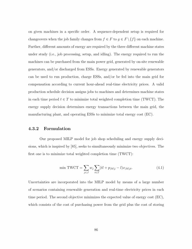
on given machines in a specific order. A sequence-dependent setup is required for

changeovers when the job family changes from f ∈ F to g ∈ F \f on each machine.

Further, different amounts of energy are required by the three different machine states

under study (i.e., job processing, setup, and idling). The energy required to run the

machines can be purchased from the main power grid, generated by on-site renewable

generators, and/or discharged from ESSs. Energy generated by renewable generators

can be used to run production, charge ESSs, and/or be fed into the main grid for

compensation according to current hour-ahead real-time electricity prices. A valid

production schedule decision assigns jobs to machines and determines machine states

in each time period t ∈ T to minimize total weighted completion time (TWCT). The

energy supply decision determines energy transactions between the main grid, the

manufacturing plant, and operating ESSs to minimize total energy cost (EC).

4.3.2 Formulation

Our proposed MILP model for job shop scheduling and energy supply deci-

sions, which is inspired by [85], seeks to simultaneously minimize two objectives. The

first one is to minimize total weighted completion time (TWCT):

min TWCT =∑j∈J

wj∑t∈T

(tl + p|M |j − l)x|M |jt. (4.1)

Uncertainties are incorporated into the MILP model by means of a large number

of scenarios containing renewable generation and real-time electricity prices in each

time period. The second objective minimizes the expected value of energy cost (EC),

which consists of the cost of purchasing power from the grid plus the cost of storing

86

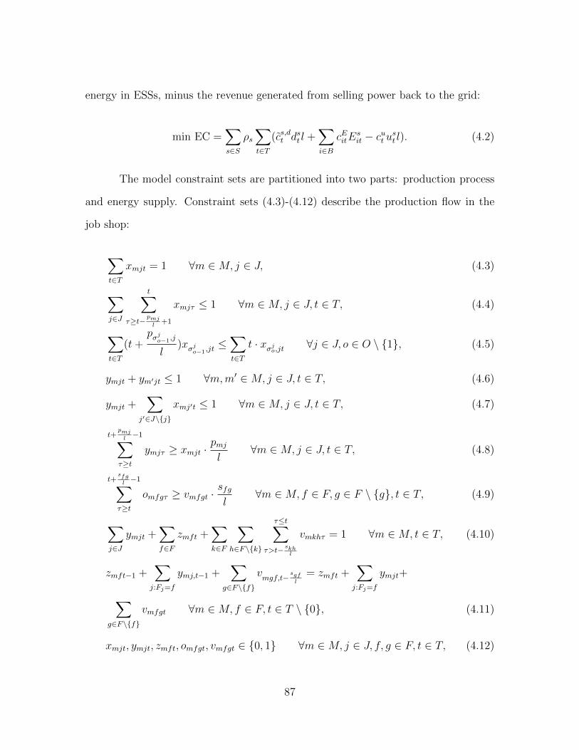
energy in ESSs, minus the revenue generated from selling power back to the grid:

min EC =∑s∈S

ρs∑t∈T

(cs,dt dst l +∑i∈B

cEitEsit − cut ust l). (4.2)

The model constraint sets are partitioned into two parts: production process

and energy supply. Constraint sets (4.3)-(4.12) describe the production flow in the

job shop:

∑t∈T

xmjt = 1 ∀m ∈M, j ∈ J, (4.3)

∑j∈J

t∑τ≥t−

pmjl

+1

xmjτ ≤ 1 ∀m ∈M, j ∈ J, t ∈ T, (4.4)

∑t∈T

(t+pσj

o−1,j

l)xσj

o−1,jt≤∑t∈T

t · xσjo,jt

∀j ∈ J, o ∈ O \ 1, (4.5)

ymjt + ym′jt ≤ 1 ∀m,m′ ∈M, j ∈ J, t ∈ T, (4.6)

ymjt +∑

j′∈J\j

xmj′t ≤ 1 ∀m ∈M, j ∈ J, t ∈ T, (4.7)

t+pmjl−1∑

τ≥t

ymjτ ≥ xmjt ·pmjl

∀m ∈M, j ∈ J, t ∈ T, (4.8)

t+sfgl−1∑

τ≥t

omfgτ ≥ vmfgt ·sfgl

∀m ∈M, f ∈ F, g ∈ F \ g, t ∈ T, (4.9)

∑j∈J

ymjt +∑f∈F

zmft +∑k∈F

∑h∈F\k

τ≤t∑τ>t− skh

l

vmkhτ = 1 ∀m ∈M, t ∈ T, (4.10)

zmft−1 +∑j:Fj=f

ymj,t−1 +∑

g∈F\f

vmgf,t−

sgfl

= zmft +∑j:Fj=f

ymjt+

∑g∈F\f

vmfgt ∀m ∈M, f ∈ F, t ∈ T \ 0, (4.11)

xmjt, ymjt, zmft, omfgt, vmfgt ∈ 0, 1 ∀m ∈M, j ∈ J, f, g ∈ F, t ∈ T, (4.12)

87

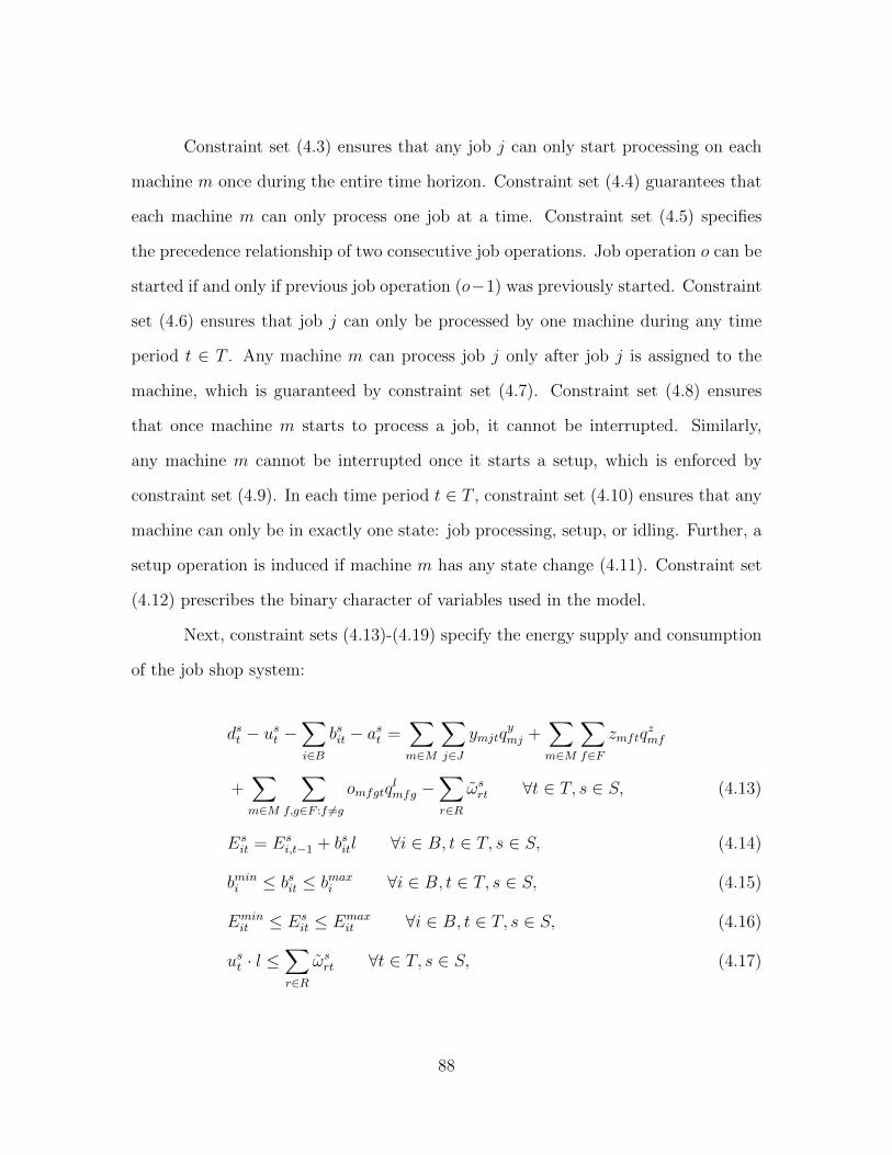
Constraint set (4.3) ensures that any job j can only start processing on each

machine m once during the entire time horizon. Constraint set (4.4) guarantees that

each machine m can only process one job at a time. Constraint set (4.5) specifies

the precedence relationship of two consecutive job operations. Job operation o can be

started if and only if previous job operation (o−1) was previously started. Constraint

set (4.6) ensures that job j can only be processed by one machine during any time

period t ∈ T . Any machine m can process job j only after job j is assigned to the

machine, which is guaranteed by constraint set (4.7). Constraint set (4.8) ensures

that once machine m starts to process a job, it cannot be interrupted. Similarly,

any machine m cannot be interrupted once it starts a setup, which is enforced by

constraint set (4.9). In each time period t ∈ T , constraint set (4.10) ensures that any

machine can only be in exactly one state: job processing, setup, or idling. Further, a

setup operation is induced if machine m has any state change (4.11). Constraint set

(4.12) prescribes the binary character of variables used in the model.

Next, constraint sets (4.13)-(4.19) specify the energy supply and consumption

of the job shop system:

dst − ust −∑i∈B

bsit − ast =∑m∈M

∑j∈J

ymjtqymj +

∑m∈M

∑f∈F

zmftqzmf

+∑m∈M

∑f,g∈F :f 6=g

omfgtqlmfg −

∑r∈R

ωsrt ∀t ∈ T, s ∈ S, (4.13)

Esit = Es

i,t−1 + bsitl ∀i ∈ B, t ∈ T, s ∈ S, (4.14)

bmini ≤ bsit ≤ bmaxi ∀i ∈ B, t ∈ T, s ∈ S, (4.15)

Eminit ≤ Es

it ≤ Emaxit ∀i ∈ B, t ∈ T, s ∈ S, (4.16)

ust · l ≤∑r∈R

ωsrt ∀t ∈ T, s ∈ S, (4.17)

88

dst , ust , E

sit, a

st ≥ 0 ∀i ∈ B, t ∈ T, s ∈ S, (4.18)

bsit unrestricted ∀i ∈ B, t ∈ T, s ∈ S. (4.19)

At any time period t, the total available power should meet total demand, according

to a power balance equation (4.13). The total available power includes power pur-

chased from the grid, power discharged from ESSs, and power generated by on-site

renewable generators. The state of ESS i is required to satisfy the governing dynam-

ics equation (4.14): the charging/discharging rate bit will be positive if the ESS i is

charging; otherwise, it is discharging. Further, these decisions are bounded by the

charging/discharging rates of the ESS (4.15). Constraint set (4.16) guarantees that

the state of the ESS is bounded by its capacity. Constraint set (4.17) ensures that

the power sold to the main grid cannot exceed the power generated by renewable

generators. While, constraint sets (4.18) - (4.19) provide variable types and limits on

the decision variables in the energy supply model, respectively.

An ε-constraint algorithm [80] is applied to the bi-objective optimization model.

We keep EC as the objective function and convert TWCT into an ε-constraint [85].

Therefore, the transformed single formulation can be reformulated as follows:

min EC =∑s∈S

ρs∑t∈T

(cs,dt dst l +∑i∈B

cEitEsit − cut ust l) (4.20)

s.t.∑j∈J

wj∑t∈T

(tl + p|M |j − l)x|M |jt ≤ ε,

(4.3) – (4.19).

89

4.4 A Hybrid Multi-objective Evolutionary Algo-

rithm

To efficiently solve the problem presented in the previous section, we develop

a hybrid multi-objective evolutionary algorithm that integrates a mathematical ap-

proach with NSGA-II [89]. Introduced by Deb et al. [89], NSGA-II is one of the best

algorithms for multi-objective problems with respect to fitness and solution diversity

([97, 98]). In our algorithm, a genetic algorithm (GA) is applied to the scheduling

part of our problem to generate feasible schedules with TWCT. Under a given fea-

sible production schedule, we use a commercial solver to compute the optimal EC,

as the energy supply problem is a linear program. Finally, fast non-dominated sort-

ing and crowding-distance approaches are applied to obtain the Pareto frontier of

non-dominated solutions.

Figure 4.1 shows a flow chart of NSGA-II. The algorithm begins with randomly

generating an initial population P0 of size N . At generation k, we have the parent

population Pk of size N . Then, the offspring population Qk of size N is generated us-

ing genetic operations such as crossover and mutation. Next, Pk and Qk are combined

to form mating pool Rk. Fast non-dominated sorting scheme is performed to classify

individuals in Rk into a non-decreasing order of fronts (F1, F2, ...) based on the in-

dividuals’ fitness. After that, individuals from the sorted list are added to the next

generation Pk+1 until the size of Pk+1 exceeds N . If the current |Pk+1|+Fi ≤ N , then

all individuals in the Fi are added to the next generation Pk+1. Otherwise, we first

sort the individuals in Fi in non-increasing order according to their crowding distance.

Then, the remaining members of Pk+1 are chosen from Fi based on their crowding

distance. Since only non-dominated individuals (lowest rank front) are selected to

add to the next generation population, elitism is ensured.

90

Start

Set k = 0, randomly generate parent population 𝑃"

Create offspring population 𝑄" of size 𝑁 usingcrossover and mutation

Combine𝑃" and 𝑄" as 𝑅" = 𝑃" ∪ 𝑄"

Perform fast non-dominated sorting to sort𝑅" and identify different fronts (F1, F2,…)

Get Pareto front from F1Meet stop criterion?

Set𝑃"01 = ∅and𝑖 = 1

𝑃"01 + 𝐹7 ≤ 𝑁

Calculate crowding distance for individuals in Fi

𝑃"01 = 𝑃"01 ∪𝐹7

Choose the first (𝑁 − 𝑃"01 )individualswithlargecrowdingdistancein𝐹7 to𝑃"01

Yes

No

Yes

No

𝑖=𝑖+

1

𝑘=𝑘+1

End

Figure 4.1: Flow chart of the NSGA-II [89]

91

4.4.1 Chromosome Representation

The GA in our proposed algorithm is used to generate job operation sequences

that are represented by chromosomes. Then, the start time of job processing and ma-

chine setups associated with these sequences are determined using a heuristic method

embedded in our evaluation process. In our algorithm, we start by sampling n ×m

U(0, 1) random numbers where n is the number of jobs and m is the number of ma-

chines. For example, when three jobs need to be processed on four machines, let the

12 randomly generated numbers be (0.6984, 0.1639, 0.1174, 0.2976, 0.5354, 0.0165,

0.2958, 0.5882, 0.7355, 0.1715, 0.8359, 0.2955). Then, we sort these random numbers

in ascending order: (0.0165, 0.1174, 0.1639, 0.1715, 0.2955, 0.2958, 0.2976, 0.5354,

0.5882, 0.6984, 0.7355, 0.8359). We record the sorted numbers’ indices as (6, 3, 2, 10,

12, 7, 4, 5, 8, 1, 9, 11). Finally, we divide each index number by the total number of

machines (four) and then round up to the next integer. Thus, the encoding for this

example is (2, 1, 1, 3, 3, 2, 1, 2, 2, 1, 3, 3). Here, 1, 2, and 3 represent job j1, j2

and j3, respectively. The different appearances of the same job j represent different

operations of the job. For example, job j1 shows up at the 2nd, 3rd, 7th, and 10th

position in the sequence, which means job j1 has four operations. The 1st appearance

of job j1 (i.e., at 2nd position) means the 1st operation (O11) of job j1. Therefore, the

corresponding job-operation sequence of the encoding sequence is (O21, O11, O12,

O31, O32, O22, O13, O23, O24, O14, O33, O34).

4.4.2 Genetic Operators

Genetic algorithms use ideas borrowed from the concepts of genetics and bio-

logical evolution. The main idea is to improve the quality of offsprings over multiple

generations. Genetic operators are used to generate more promising candidate solu-

92

tions that replace less promising solutions. In our algorithm, crossover and mutation

operators are employed.

Crossover - Crossover is performed on two parent chromosomes that are ran-

domly selected from the population. In our algorithm, we adopt a random two-point

crossover operator. Two crossover points are randomly chosen from the parent chro-

mosomes. Then, genes in between the two points are swapped between the parent

chromosomes (Figure 4.2). Thus, two child chromosomes are obtained.

0.6984 0.1639 0.1174 0.2976 0.5354 0.0165 0.2958 0.5882 0.7355 0.1715 0.8359 0.2955

0.2004 0.8668 0.0731 0.5703 0.4241 0.3424 0.1863 0.7934 0.8901 0.7585 0.3345 0.5788

Parent 1

Parent 2

0.6984 0.1639 0.1174 0.2976 0.4241 0.3424 0.1863 0.7934 0.8901 0.1715 0.8359 0.2955

0.2004 0.8668 0.0731 0.5703 0.5354 0.0165 0.2958 0.5882 0.7355 0.7585 0.3345 0.5788

Child 1

Child 2

Figure 4.2: Example crossover operation

Mutation - Mutation preserves genetic variation with the intent to escape from

local minima. It involves selecting a chromosome and two points at random, and then

generating new U(0, 1) genes at these points (Figure 4.3).

0.6984 0.1639 0.1174 0.2976 0.5354 0.0165 0.2958 0.5882 0.7355 0.1715 0.8359 0.2955Parent

0.6984 0.2344 0.1174 0.2976 0.5354 0.0165 0.2958 0.5882 0.7355 0.4692 0.8359 0.2955Child

Figure 4.3: Example mutation operation

4.4.3 Heuristic Objective Functions

As described in Section 4.3, the model decomposes into two parts: (1) job shop

scheduling decisions with constraint sets (4.3)-(4.12) and (2) energy supply decisions

93

with constraint sets (4.13)-(4.19). For the job shop problem, given the job operation

sequences decoded from our chromosome, we created a heuristic method to gener-

ate the start times of both job processing and machine setups between different job

families. As a result, TWCT can be calculated for any chromosome. The EC objec-

tive function is computed optimally using our mathematical model after production

schedule is fixed in the model as an input. Our heuristic method uses five approaches

to generate job start times on machines.

1 Earliest start time: Algorithm 1 describes the earliest start time method. Each

job operation is required to be started as early as possible within the time

horizon while respecting job operation sequences and machine availability re-

Algorithm 1 Algorithm of earliest start time

1: Input: decoded job operation sequence2: for i = the first job operation to the last job operations do3: if tj ≤ tm then4: tstart ← tj5: else6: tstart ← tm7: end if8: tm = tj ← tstart+ job j’s processing time on machine m9: on machine m, find job operation i’s job family f and its next job operationi′’s job family g

10: if i is not the last job operation assigned on machine m then11: tcomp ← tm12: the start time of setup tStartSetup ← tm13: the completion time of setup tCompSetup ← tm+ setup time between job

family f and g14: Record tstart, tcomp, tStartSetup, and tCompSetup15: else16: tcomp ← tm17: Record tstart and tcomp18: end if19: tm ← tm+ setup time between job family f and g20: end for

94

quirements. In addition, all job family-related setup operations are performed

at the earliest possible time.

2 Latest start time: In this method, we assign job operations to begin processing

as late as possible. Given a job operation sequence, our algorithm starts from

the last job operation and progresses to the first one, placing each hob as late

in the schedule as possible (Algorithm 2). As was the case in Algorithm 1, all

job operations, machine availability, and setup requirements are enforced.

Methods 3 - 5 are similar to the earliest start time (method 1). The difference

lies in generating the starting time of job operations (lines 3-6, Algorithm 1). Besides

the decoded job operation sequence, methods 3 - 5 also require as input the latest

Algorithm 2 Algorithm of latest start time

1: Input: decoded job operation sequence2: for i = the #of job operations to the first job operation do3: if tj ≤ tm then4: tcomp ← tj5: else6: tcomp ← tm7: end if8: tm = tj ← tcomp− job j’s processing time on machine m9: on machine m, find job operation i’s job family g and its previous job operationi′’s job family f

10: if i is not the first job operation assigned on machine m then11: tstart ← tm12: the completion time of setup tCompSetup ← tm13: the start time of setup tStartSetup ← tm− setup time between job family f

and g14: Record tstart, tcomp, tStartSetup, and tCompSetup15: else16: tstart ← tm17: Record tstart and tcomp18: end if19: tm ← tm− setup time between job family f and g20: end for

95

start time of each job operation (which can be obtained from method 2).

3 Lowest price start time: This method seeks to find the time period with the

lowest electricity price, which is denoted as tLowestPrice, within time window [tj,

the latest start time of job operation i] if job j becomes available before machine

m (Algorithm 3). Otherwise, find tLowestPrice within time window [tm, the latest

start time of job operation i] and set start time tstart equal to tLowestPrice.

4 Highest renewable generation start time: Similar to method 3, this method seeks

the time period with the highest renewable generation thighestRenewable within

time period [tj, the latest start time of job operation i] or [tm, the latest start

Algorithm 3 Algorithm of start time with the lowest price

1: Input: decoded job operation sequence2: for i = the first job operation to the last job operations do3: if tj ≤ tm then4: tstart ← the time period with the average lowest electricity price within

time window [tj, the latest start time of job operation i]5: else6: tstart ← the time period with the average lowest electricity price within

time window [tm, the latest start time of job operation i]7: end if8: tm = tj ← tstart+ job j’s processing time on machine m9: on machine m, find job operation i’s job family f and its next job operationi′’s job family g

10: if i is not the last job operation assigned on machine m then11: tcomp ← tm12: the start time of setup tStartSetup ← tm13: the completion time of setup tCompSetup ← tm+ setup time between job

family f and g14: Record tstart, tcomp, tStartSetup, and tCompSetup15: else16: tcomp ← tm17: Record tstart and tcomp18: end if19: tm ← tm+ setup time between job family f and g20: end for

96

time of job operation i], based on whether tj ≥ tm or tj < tm, respectively.

5 Random start time: Within time window [tj, the latest start time of job op-

eration i] or [tm, the latest start time of job operation i], start time tstart is

randomly generated in this method.

In all of the five methods, any required setup between two job operations on

a machine is scheduled right after the first job operation is completed. Thus, the

start time of the setup is as early as possible. To improve solution diversity, we also

randomly generate setup start times for the schedules obtained by the five methods.

With 50% probability, we generate a start time for a setup within the time frame of

its earliest start time and latest start time. The earliest start time is equal to the

completion time of job operation i and the latest start time is equal to the start time

of i′ minus the setup time between i and i′.

4.4.4 Fast non-dominated sorting and crowding distance

Fast non-dominated sorting and crowding distance are two main features of

NSGA-II which are used to evaluate each solution in Rk as shown in Figure 4.1.

Let np and Sp denote the number of solutions that dominate solution p and a set

of solutions that the solution p dominates, respectively. First, we put all solutions

with np = 0 in the first non-dominated front F1. Then, for each solution in F1, we

visit each individual q in its set Sq and reduce nq by one. If any individual q’s nq

becomes 0, we put it into a new non-dominated front. This process continues until

all individuals are considered and all fronts are identified. We refer the reader to [89]

for a detailed exposition of the fast non-dominated sorting scheme.

The crowding distance measure first sorts individual solutions in front Fk in

non-decreasing order of the nth objective function value. The crowding distance CDin

97

of each solution i with respect to objective n is calculated as:

CDin =fn(i+ 1)− fn(i− 1)

fmaxn − fminn

, (4.21)

where fmaxn and fminn are the maximum and minimum values of the nth objective

function of the solution. The boundary solutions (solutions with the smallest and

largest objective function value) are assigned to an infinite distance value. The total

crowding distance of each solution i is calculated as:

CDi =N∑n=1

CDin, (4.22)

where N is the number of objectives.

4.5 Computational Experiments

To test the performance of our proposed mathematical model and algorithm,

30 instances are generated (Table 4.1). We consider three different sets of jobs (3, 6,

and 9) processed on three machines in the 30 instances and two sets of time periods:

24 and 96. As each day has 24 hours, the length of each time period is 1 hour (15

minutes) when there are 24 (96) time periods. Table 4.2 provides the values of other

scheduling-related parameters in the test instances.

Renewable generation data is from [85] wherein solar generation data is adopted.

The hour-ahead real-time pricing scheme is derived from the Commonwealth Edison

(ComEd) company [99]. To illustrate the problem under study and our algorithms,

we generate four scenarios, each with an equal probability of occurrence. The feed-

in electricity price is set to 0.08923 USD/kWh as found in the Electric-Renewable

Market Adjusting Tariff of the Pacific Gas and Electric Company [84]. One ESS is

98

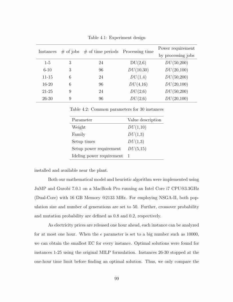
Table 4.1: Experiment design

Instances # of jobs # of time periods Processing timePower requirement

by processing jobs

1-5 3 24 DU(2,6) DU (50,200)

6-10 3 96 DU (10,30) DU (20,100)

11-15 6 24 DU (1,4) DU (50,200)

16-20 6 96 DU (4,16) DU (20,100)

21-25 9 24 DU (2,6) DU (50,200)

26-30 9 96 DU (2,6) DU (20,100)

Table 4.2: Common parameters for 30 instances

Parameter Value description

Weight DU (1,10)

Family DU (1,3)

Setup times DU (1,3)

Setup power requirement DU (5,15)

Ideling power requirement 1

installed and available near the plant.

Both our mathematical model and heuristic algorithm were implemented using

JuMP and Gurobi 7.0.1 on a MacBook Pro running an Intel Core i7 CPU@3.3GHz

(Dual-Core) with 16 GB Memory @2133 MHz. For employing NSGA-II, both pop-

ulation size and number of generations are set to 50. Further, crossover probability

and mutation probability are defined as 0.8 and 0.2, respectively.

As electricity prices are released one hour ahead, each instance can be analyzed

for at most one hour. When the ε parameter is set to a big number such as 10000,

we can obtain the smallest EC for every instance. Optimal solutions were found for

instances 1-25 using the original MILP formulation. Instances 26-30 stopped at the

one-hour time limit before finding an optimal solution. Thus, we only compare the

99

mathematical model and our proposed algorithm using the smallest EC. Let ∆ denote

the gap between the EC obtained from the mathematical model and the NSGA-II

such that ∆ = (ECNSGA−II − ECMILP )/ECNSGA−II . Table 4.3 summarizes results

from the two solution methods. Our NSGA-II algorithm can produce competitive

solutions with an average ∆ = 3.29% compared to the mathematical model. When

the number of jobs increases from 3 to 6 and then to 9, the average solution gap ∆

increases from 1.5% to 2.14%, and then to 6.22%. Similarly, ∆ increases from 1.73%

to 4.85% as the number of time periods increases from 24 to 96.

Overall, the quality of our NSGA-II-based solutions decreases as problem in-

stances become more complicated. However, NSGA-II can produce solutions fairly

quickly, especially for large problems. The 5th column in Table 4.3 provides the so-

lution time of the mathematical model. These times are only for one ε parameter.

Tens or 100s of ε parameters need to be considered for each instance for full Pareto

results. When there are nine jobs and 96 time periods considered in a job shop, the

MILP cannot determine an optimal solution, even for only one ε parameter within

one hour. In contrast, our NSGA-II algorithm can produce all Pareto frontiers of

non-dominated solutions within 1700s (6th column in Table 4.3).

The algorithm presented in section 4.4 considers five methods simultaneously

to generate schedules (NSGA-II 5). Now, we modify the algorithm by randomly

selecting one method to generate a schedule for each chromosome, which is denoted

as NSGA-II 1. Tabel 4.4 summarizes the results of solutions produced by NSGA-

II 1. Here, ∆ is the gap between the EC obtained from the mathematical model

and NSGA-II 1. On average, the ∆ is 4.36% for all 30 instances. The gap between

EC obtained from NSGA-II 5 and NSGA-II 1 is 1.14%. However, the running time

reduces 716.24s (83.6%) on average, when choosing NSGA-II 1.

Now, we further examine the performance of NSGA-II 5 and NSGA-II 1. To

100

Table 4.3: Mathematical Model vs. NSGA-II

InstanceEC ($) Running time (s)

MILP NSGA-II ∆ MILP NSGA-II

1 773.789 789.773 2.02% 6.27 810.19

2 649.518 654.647 0.78% 9.31 192.61

3 548.143 557.496 1.68% 7.68 209.93

4 623.966 644.218 3.14% 6.31 605.90

5 634.242 634.277 0.01% 6.11 657.16

6 225.175 230.588 2.35% 37.65 1371.40

7 356.036 361.631 1.55% 33.85 1322.77

8 279.760 280.597 0.30% 29.25 1390.68

9 210.707 217.21 2.99% 31.98 1194.64

10 252.472 252.988 0.20% 9.61 1139.29

11 872.868 885.939 1.48% 21.91 205.31

12 890.330 890.619 0.03% 25.39 844.72

13 850.172 858.564 0.98% 47.43 699.99

14 777.846 779.683 0.24% 48.10 891.76

15 859.454 870.203 1.24% 53.75 784.82

16 339.162 349.449 2.94% 1376.53 1525.95

17 229.493 239.206 4.06% 1071.31 1535.39

18 270.511 279.15 3.09% 3607.25 1647.76

19 354.436 368.287 3.76% 1259.32 1497.42

20 223.755 232.055 3.58% 2064.15 1697.14

21 895.048 918.938 2.60% 191.07 220.87

22 907.968 938.514 3.25% 293.19 221.76

23 789.433 815.575 3.21% 199.80 229.95

24 965.238 984.047 1.91% 785.38 215.24

25 964.817 997.933 3.32% 19.17 245.32

26 422.372 456.407 7.46% 3606.24 667.78

27 129.445 134.936 4.07% 3623.14 1691.38

28 97.965 107.953 9.25% 3606.57 690.49

29 50.227 60.7778 17.36% 3606.29 692.64

30 114.298 126.686 9.78% 3605.86 597.24

101

Tab

le4.

4:Sol

uti

onre

sult

sof

NSG

A-I

I1

Inst

ance

EC

($)

∆R

unnin

gti

me

(s)

Inst

ance

EC

($)

∆R

unnin

gti

me

(s)

184

1.75

48.

07%

57.2

716

349.

158

2.86

%23

5.55

266

4.27

72.

22%

61.6

017

242.

441

5.34

%20

5.22

359

2.38

27.

47%

64.6

618

286.

689

5.64

%21

1.79

464

7.64

23.

66%

64.6

619

371.

365

4.56

%21

2.46

564

7.79

42.

09%

68.4

520

237.

626

5.84

%20

7.98

623

0.58

82.

35%

188.

4621

939.

473

4.73

%75

.70

736

4.56

42.

34%

187.

3322

942.

778

3.69

%91

.43

828

0.97

60.

43%

191.

3823

821.

843

3.94

%68

.02

922

0.81

54.

58%

184.

6324

987.

215

2.23

%73

.14

1025

2.98

80.

20%

191.

7225

1010

.210

4.49

%73

.42

1188

2.58

31.

10%

72.9

326

448.

027

5.73

%20

9.68

1289

0.61

90.

03%

143.

0727

137.

361

5.76

%21

9.54

1386

5.54

41.

78%

68.6

428

109.

427

10.4

7%21

7.22

1478

8.40

91.

34%

65.5

929

60.9

4517

.59%

214.

85

1586

5.56

80.

71%

70.2

730

126.

519.

65%

213.

55

102

have a better understanding of solution quality, we combine all Pareto solutions of

a problem instance into a new set of non-dominated solutions called a super front.

Let N(T ) be the number of Pareto front solutions and N(H) be the number of

non-dominated solutions produced by an algorithm in the aggregated set. The per-

formance ratio of a particular algorithm H, PR(H) = N(H)N(T )

. As Table 4.5 shows,

NSGA-II 5 performs better than NSGA-II 1 for 23 of the 30 instances. The average

performance ratios of NSGA-II 5 and NSGA-II 1 are 74.24% and 34.67%, respectively.

Table 4.5: Performance ratios of NSGA-II 5 and NSGA-II 1

Instance NSGA-II 5 NSGA-II 1 Instance NSGA-II 5 NSGA-II 1

1 87.5% 25.0% 16 87.5% 87.5%

2 85.7% 28.6% 17 100.0% 0.0%

3 100.0% 14.3% 18 88.9% 11.1%

4 66.7% 44.4% 19 66.7% 33.3%

5 100.0% 0.0% 20 75.0% 25.0%

6 50.0% 100.0% 21 100.0% 0.0%

7 71.4% 28.6% 22 40.0% 60.0%

8 90.0% 30.0% 23 55.6% 44.4%

9 100.0% 7.7% 24 53.3% 46.7%

10 50.0% 83.3% 25 100.0% 0.0%

11 83.3% 16.7% 26 27.8% 72.2%

12 100.0% 28.6% 27 100.0% 0.0%

13 62.5% 25.0% 28 26.1% 69.6%

14 100.0% 0.0% 29 83.3% 11.1%

15 66.7% 83.3% 30 22.7% 63.6%

We now use instances 1 and 11 to illustrate how we calculate the performance

ratio. Figure 4.4 shows the plot of non-dominated solutions of NSGA-II 5, along

with solutions achieved with NSGA-II 1, for the example problem instances. Initially,

NSGA-II 5 and NSGA-II 1 generate eight and five Pareto solutions for instance 1,

respectively. Among all eight Pareto solutions for instance 1, NSGA-II 1 has one

103

same solution (188, 850.527) as NSGA-II 5 does and one non-dominated solution at

(200, 842.363). Besides the shared solution (188, 850.527), NSGA-II 5 provides six

additional non-dominated solutions. Therefore, the performance ratios of NSGA-II 5

and NSGA-II 1 are 87.5%(7/8) and 25%(2/8), respectively. For instance 11, 10 of

12 and 2 of 12 non-dominated solutions are obtained by NSGA-II 5 and NSGA-II 1,

respectively, which result in performance ratios of 83.3% and 16.7%. The purpose of

generating a super front is to let decision-makers evaluate trade-offs between different

solution options effectively [97].

200 220 240 260

TWCT (hr)

780

800

820

840

860

EC

(U

SD

)

NSGA-II_5

NSGA-II_1

(a) Pareto fronts of instance 1

340 360 380 400 420 440 460

TWCT (hr)

880

890

900

910

920

930

940

950

EC

(U

SD

)NSGA-II_5

NSGA-II_1

(b) Pareto fronts of instance 11

Figure 4.4: Pareto fronts of instance 1 and 11

4.6 Conclusions and Future Research

In this paper, we study a job shop scheduling problem with on-site renewable

generation and an energy storage system under hour-ahead real-time pricing schemes

to simultaneously minimize the total weighted completion time and energy costs. Our

model is formulated as a time-indexed, mixed-integer linear program. To solve the

problem, we adopt an ε-constraint approach to transform TWCT into an ε−constraint

and minimize energy costs. To improve computational efficiency, we develop a hybrid

104

multi-objective evolutionary algorithm based on NSGA-II [89]. Five methods are

embedded in the algorithm to generate production schedules. Then, under a given

feasible production schedule, energy costs are calculated by a commercial solver.

Experimental results confirm that both mathematical modeling and our devel-

oped algorithm are competitive. The gap between the EC obtained from the MILP

and our NSGA-II is 3.29%, on average. For large problem instances (nine jobs and

96 time periods), the MILP cannot obtain optimal solution for even one ε parameter

within a one-hour time limit. In contrast, our heuristic algorithm can produce all

Pareto fonts within 1700 seconds for any instance. Using sets of Pareto optimal solu-

tions, decision-makers can choose the desired solution according to their preferences to

determine production schedules and energy requirements. Computational tests also

show that NSGA-II 1 can produce solutions more quickly than NSGA-II 5, but with

slightly lower quality. This result indicates that both NSGA-II 5 and NSGA-II 1 can

be used as managerial tools to provide solutions on minimizing production scheduling

and energy cost simultaneously with regards to hour-ahead real-time electricity pric-

ing scheme and stochastic renewable generation. However, there is a trade-off between

solution quality and computational time that decision-makers must consider.

Future studies can investigate how production schedules and energy supply

decisions change with different pricing schemes. Other objective functions also can

be studied such as minimizing greenhouse gas emissions. Another interesting research

topic could be to examine the performance of other heuristic methods such as Tabu

search on the problem of interest.

105

Chapter 5

Conclusions and Future Research

With energy shortage and environmental challenges becoming increasingly se-

vere problems, interest in renewable energy resources has grown in recent years. This

dissertation considers utilizing renewable energy resources in two major locations: the

power grid side and the end-use customer side of power systems. As renewable energy

resources like solar and wind energy typically fluctuate with weather variations, the

inherent stochastic nature of renewable energy resources makes the decision making

of utilizing renewable generation complex. To this end, we study how to effectively

utilize renewable energy in power systems.

5.1 Research Conclusions

In the first phase of this dissertation, we focus on managing energy of net-

worked microgrids in a power grid with the integration of renewable energy resources.

A centralized arbiter in the main grid regulates power generation and supply for the

whole power system. Each microgrid contains various energy management settings,

and as an agent, seeks to minimize cost within the microgrid area after receiving

106

the arbiter’s decision and an observation of the renewable generation and customer

demand. We present a two-stage stochastic optimization framework for this multi-

agent system by extending the classical 2-SP model to include multiple subproblems.

To the best of our knowledge, this is the first study that investigates multiple sub-

problems with heterogeneous decisions and stochastic processes in the second-stage.

To optimize this energy management problem, we develop stochastic decomposition-

based algorithms. Compared to the benchmark 2-SD approach, our algorithm can

provide reliable overall cost estimates to the proposed problem with 50% less solution

time. Both of our proposed approximation approaches, which are agent cuts (MA-

SD(m)) and aggregated cuts (MA-SD(a)), yield statistically comparable results, but

MA-SD(a) is computationally more efficient.

In the second phase, we focus on studying renewable generators installed and

available in a flow shop. A two-stage, multi-objective stochastic MILP is developed

for the flow shop scheduling problem with energy decisions. In the first stage, a time-

indexed MILP is proposed to minimize total weighted completion time. The second

stage determines the energy supply decisions according to the production schedule

and a realization of renewable energy generation to minimize energy costs under a

TOU electricity price scheme. First, we employ a ε-constraint approach to transform

the multi-objective problem into a two-stage, single-objective stochastic MILP which

is then solved by an L-shaped method. In our experiments, a set of Pareto optimal

solutions are provided for decision-makers to minimize total weighted completion

time and energy costs in scheduling the production process. Decision-makers can

choose a solution according to their preference among all Pareto optimal solutions.

Our experiments show that although using solar generation or wind generation can

reduce energy costs, using solar energy can reduce more cost than using wind energy

for the problem under study.

107

In the third and final phase of this dissertation, we extend the flow shop

scheduling with on-site renewable generation problem to a job shop environment. We

present a time-indexed, mixed-integer linear program to simultaneously minimize the

total weighted completion time and energy costs under hour-ahead real-time pricing

schemes. An ε-constraint approach is used to transform the total weighted completion

time into an ε− constraint and minimize energy costs. Since the problem is NP-hard,

we develop a hybrid multi-objective evolutionary algorithm based on NSGA-II to

improve computational efficiency. First, production schedules are generated using five

methods which are embedded in the algorithm. Then, energy costs are calculated by

a commercial solver under a given feasible production schedule. Computational tests

show that both mathematical modeling and our developed algorithm are competitive.

However, our heuristic algorithm can produce all Pareto fonts more quickly than the

MILP. When used as a managerial tool, our algorithm reveals trade-offs between

solution quality and computational time that decision makers must consider.

5.2 Future Research Directions

There are a number of research opportunities in the future that could enhance

this research study. In Chapter 2, the structure of our algorithm involves solving

several independent subproblems (corresponding to MGs) that is naturally fit for a

distributed/parallel computing implementation. Bi-direction transactions can be in-

vestigated in a smart grid in which microgrids not only purchase power from the main

grid but also can sell power back to the grid to increase the utilization of renewable

energy over the entire power system. Further, transactions between microgrids also

could be addressed.

For the scheduling problems with on-site renewable energy in Chapters 3 and

108

4, different objective functions such as due-date related lateness can be investigated.

In addition, comparisons of production schedules and energy supply changes under

different pricing schemes can be studied. Different time horizon lengths also need to be

investigated as not all manufacturing facilities work 24 hours per day. Finally, another

interesting research topic could be to examine the performance of other heuristic

methods such as Tabu search on the problem of interest.

109

Bibliography

[1] J. R. Birge and F. Louveaux, Introduction to stochastic programming. SpringerScience & Business Media, 2011.

[2] M. Shahidehpour and J. F. Clair, “A functional microgrid for enhancing reliabil-ity, sustainability, and energy efficiency,” The Electricity Journal, vol. 25, no. 8,pp. 21–28, 2012.

[3] F. M. P. Junior, A. C. Z. de Souza, M. Castilla, D. Q. Oliveira, P. F. Ribeiro et al.,“Control strategies for improving energy efficiency and reliability in autonomousmicrogrids with communication constraints,” Energies, vol. 10, no. 9, pp. 1–16,2017.

[4] D. T. Ton and M. A. Smith, “The US department of energy’s microgrid initia-tive,” The Electricity Journal, vol. 25, no. 8, pp. 84–94, 2012.

[5] N. Hamsic, A. Schmelter, A. Mohd, E. Ortjohann, E. Schultze, A. Tuckey, andJ. Zimmermann, “Increasing renewable energy penetration in isolated grids usinga flywheel energy storage system,” in 2007 International Conference on PowerEngineering, Energy and Electrical Drives. IEEE, 2007, pp. 195–200.

[6] I. Stadler, “Power grid balancing of energy systems with high renewable energypenetration by demand response,” Utilities Policy, vol. 16, no. 2, pp. 90–98,2008.

[7] A. Evans, V. V. Strezov, and T. J. Evans, “Assessment of utility energy storageoptions for increased renewable energy penetration,” Renewable and SustainableEnergy Reviews, vol. 16, no. 6, pp. 4141–4147, 2012.

[8] C. Bueno and J. A. Carta, “Wind powered pumped hydro storage systems, ameans of increasing the penetration of renewable energy in the Canary Islands,”Renewable and Sustainable Energy Reviews, vol. 10, no. 4, pp. 312–340, 2006.

[9] R. Segurado, G. Krajacic, N. Duic, and L. Alves, “Increasing the penetration ofrenewable energy resources in S. Vicente, Cape Verde,” Applied Energy, vol. 88,no. 2, pp. 466–472, 2011.

110

[10] M. L. Pinedo, Scheduling: Theory, Algorithms, and Systems. Springer, 2015.

[11] B. Eksioglu, S. D. Eksioglu, and P. Jain, “A tabu search algorithm for the flow-shop scheduling problem with changing neighborhoods,” Computers & IndustrialEngineering, vol. 54, no. 1, pp. 1–11, 2008.

[12] S. Mason, S. Jin, and C. Wessels, “Rescheduling strategies for minimizing totalweighted tardiness in complex job shops,” International Journal of ProductionResearch, vol. 42, no. 3, pp. 613–628, 2004.

[13] M. L. Bell and D. L. Davis, “Reassessment of the lethal london fog of 1952: novelindicators of acute and chronic consequences of acute exposure to air pollution.”Environmental health perspectives, vol. 109, no. Suppl 3, p. 389, 2001.

[14] Y. Chen, S. Lu, Y. Chang, T. Lee, and M. Hu, “Economic analysis and optimalenergy management models for microgrid systems: A case study in Taiwan,”Applied Energy, vol. 103, pp. 145–154, 2013.

[15] P. Basak, S. Chowdhury, S. Halder nee Dey, and S.P. Chowdhury, “A literaturereview on integration of distributed energy resources in the perspective of con-trol, protection and stability of microgrid,” Renewable and Sustainable EnergyReviews, vol. 16, no. 8, pp. 5545–5556, 2012.

[16] R. H. Lasseter, “MicroGrids,” in 2002 IEEE Power Engineering Society WinterMeeting. Conference Proceedings (Cat. No.02CH37309), vol. 1, 2002, pp. 305–308.

[17] A. Zakariazadeh, J. Shahram, and P. Siano, “Smart microgrid energy and reservescheduling with demand response using stochastic optimization,” InternationalJournal of Electrical Power & Energy Systems, vol. 63, pp. 523–533, 2014.

[18] T. Ackermann, G. Andersson, and L. Soder, “Distributed generation: a defini-tion,” Electric Power Systems Research, vol. 57, no. 3, pp. 195–204, 2001.

[19] H. Gangammanavar and S. Sen, “Two-scale stochastic optimization for control-ling distributed storage devices,” IEEE Transactions on Smart Grid, vol. 9, no. 4,pp. 2691–2702, 2016.

[20] M. Marzband, N. Parhizi, M. Savaghebi, and J. M. Guerrero, “Distributed smartdecision-making for a multimicrogrid system based on a hierarchical interactivearchitecture,” IEEE Transactions on Energy Conversion, vol. 31, no. 2, pp. 637–648, 2016.

[21] A. R. Malekpour and A. Pahwa, “Stochastic energy management in distributionsystems with correlated wind generators,” IEEE Transactions on Power Systems,2017.

111

[22] K. Boroojeni, M. H. Amini, A. Nejadpak, T. Dragicevic, S. S. Iyengar, andF. Blaabjerg, “A novel cloud-based platform for implementation of obliviouspower routing for clusters of microgrids,” Ieee Access, vol. 5, pp. 607–619, 2017.

[23] Z. Wang, B. Chen, J. Wang, M. M. Begovic, and C. Chen, “Coordinated energymanagement of networked microgrids in distribution systems,” IEEE Transac-tions on Smart Grid, vol. 6, no. 1, pp. 45–53, 2015.

[24] H.S.V.S. Kumar Nunna and S. Doolla, “Multiagent-based distributed-energy-resource management for intelligent microgrids,” IEEE Transactions on Indus-trial Electronics, vol. 60, no. 4, pp. 1678–1687, 2013.

[25] T. Logenthiran, D. Srinivasan, and A. M. Khambadkone, “Multi-agent systemfor energy resource scheduling of integrated microgrids in a distributed system,”Electric Power Systems Research, vol. 81, no. 1, pp. 138–148, 2011.

[26] T. Dai and W. Qiao, “Trading wind power in a competitive electricity market us-ing stochastic programing and game theory,” IEEE Transactions on SustainableEnergy, vol. 4, no. 3, pp. 805–815, 2013.

[27] S. W. Wallace and S.-E. Fleten, “Stochastic programming models in energy,”Handbooks in operations research and management science, vol. 10, pp. 637–677,2003.

[28] A. Sheikhi, A. Maani, and A. Ranjbar, “Evaluation of intelligent distributionnetwork response to plug-in hybrid electric vehicles,” in PowerTech (POW-ERTECH), 2013 IEEE Grenoble. IEEE, 2013, pp. 1–6.

[29] D. T. Nguyen and L. B. Le, “Optimal energy management for cooperative micro-grids with renewable energy resources,” in 2013 IEEE International Conferenceon Smart Grid Communications (SmartGridComm). IEEE, 2013, pp. 678–683.

[30] Y. M. Ding, S. H. Hong, and X. H. Li, “A demand response energy managementscheme for industrial facilities in smart grid,” IEEE Transactions on IndustrialInformatics, vol. 10, no. 4, pp. 2257–2269, 2014.

[31] G. Goddard, J. Klose, and S. Backhaus, “Model development and identificationfor fast demand response in commercial HVAC systems,” IEEE Transactions onSmart Grid, vol. 5, no. 4, pp. 2084–2092, 2014.

[32] N. Li, L. Chen, and S. H. Low, “Optimal demand response based on utilitymaximization in power networks,” in 2011 IEEE power and energy society generalmeeting. IEEE, 2011, pp. 1–8.

[33] Z. Chen, L. Wu, and Y. Fu, “Real-time price-based demand response manage-ment for residential appliances via stochastic optimization and robust optimiza-tion,” IEEE Transactions on Smart Grid, vol. 3, no. 4, pp. 1822–1831, 2012.

112

[34] P. Zhao, S. Suryanarayanan, and M. G. Simoes, “An energy management systemfor building structures using a multi-agent decision-making control methodol-ogy,” IEEE Transactions on Industry Applications, vol. 49, no. 1, pp. 322–330,2013.

[35] R. de Dear and G. S. Brager, “The adaptive model of thermal comfort and energyconservation in the built environment,” International Journal of Biometeorology,vol. 45, no. 2, pp. 100–108, 2001.

[36] D. J. Sailor and A. A. Pavlova, “Air conditioning market saturation and long-term response of residential cooling energy demand to climate change,” Energy,vol. 28, no. 9, pp. 941–951, 2003.

[37] Y. Agarwal, B. Balaji, R. Gupta, J. Lyles, M. Wei, and T. Weng, “Occupancy-driven energy management for smart building automation,” in Proceedings ofthe 2nd ACM Workshop on Embedded Sensing Systems for Energy-Efficiency inBuilding. ACM, 2010, pp. 1–6.

[38] A. Etxeberria, I. Vechiu, H. Camblong, and J. M. Vinassa, “Hybrid energy stor-age systems for renewable energy sources integration in microgrids: A review,”in IPEC, 2010 Conference Proceedings. IEEE, 2010, pp. 532–537.

[39] P. Denholm, E. Ela, B. Kirby, and M. Milligan, “The role of energystorage with renewable electricity generation. NREL/TP-6A247187. NationalRenewable Energy Laboratory,” 2010, Accessed: 2020-1-5. [Online]. Available:https://www.nrel.gov/docs/fy10osti/47187.pdf

[40] R. Sioshansi, P. Denholm, and T. Jenkin, “Market and policy barriers to deploy-ment of energy storage,” Economics of Energy & Environmental Policy, vol. 1,no. 2, pp. 47–63, 2012.

[41] A. L. Motto, F. D. Galiana, A. J. Conejo, and J. M. Arroyo, “Network-constrained multiperiod auction for a pool-based electricity market,” IEEETransactions on Power Systems, vol. 17, no. 3, pp. 646–653, 2002.

[42] J. F. Benders, “Partitioning procedures for solving mixed-variables programmingproblems,” Numerische Mathematik, vol. 4, no. 1, pp. 238–252, 1962.

[43] G. B. Dantzig and P. Wolfe, “Decomposition principle for linear programs,”Operations Research, vol. 8, no. 1, pp. 101–111, 1960.

[44] R. T. Rockafellar and R. J. B. Wets, “Scenarios and policy aggregation in opti-mization under uncertainty,” Mathematics of Operations Research, vol. 16, no. 1,pp. 119–147, 1991.

113

[45] H. Gangammanavar, S. Sen, and V. M. Zavala, “Stochastic optimization of sub-hourly economic dispatch with wind energy,” IEEE Transactions on Power Sys-tem, vol. 31, no. 2, pp. 949–959, 2015.

[46] S. Sen and Y. Liu, “Mitigating uncertainty via compromise decisions in two-stage stochastic linear programming: Variance reduction,” Operations Research,vol. 64, no. 6, pp. 1422–1437, 2016.

[47] J. Higle and S. Sen, “Finite master programs in regularized stochastic decompo-sition,” Mathematical Programming, vol. 67, no. 1-3, pp. 143–168, 1994.

[48] J. E. Price and J. Goodin, “Reduced network modeling of WECC as a marketdesign prototype,” in 2011 IEEE Power and Energy Society General Meeting.IEEE, 2011, pp. 1–6.

[49] National Renewable Energy Laboratory (NREL), “Western wind andsolar integration study,” Accessed: 2020-1-5. [Online]. Available: https://www.nrel.gov/grid/wwsis.html

[50] U.S. Energy Information Administration (EIA), “Levelized cost and levelizedavoided cost of new generation resources in the annual energy outlook 2015,”Accessed: 2020-1-5. [Online]. Available: https://www.eia.gov/outlooks/archive/aeo

[51] J. L. Higle and S. Sen, “Duality and statistical tests of optimality for two stagestochastic programs,” Mathematical Programming, vol. 75, no. 2, pp. 257–275,1996.

[52] U.S. Energy Information Administration (EIA), “Use of energy explained,”Accessed: 2020-1-5. [Online]. Available: https://www.eia.gov/energyexplained/use-of-energy/industry.php

[53] U.S. Energy Information Administration (EIA), “EIA monthly energy review,”Accessed: 2020-1-5. [Online]. Available: https://www.eia.gov/totalenergy/data/monthly/pdf/mer.pdf

[54] S. Wang, H. Gangammanavar, S. D. Eksioglu, and S. J. Mason, “Stochasticoptimization for energy management in power systems with multiple microgrids,”IEEE Transactions on Smart Grid, vol. 10, no. 1, pp. 1068–1079, 2019.

[55] A. Sharma, F. Zhao, and J. W. Sutherland, “Econological scheduling of a man-ufacturing enterprise operating under a time-of-use electricity tariff,” Journal ofCleaner Production, vol. 108, pp. 256–270, 2015.

[56] U.S. Energy Information Administration (EIA), “International Energy Outlook2017,” Accessed: 2020-9-8. [Online]. Available: https://www.eia.gov/outlooks/ieo/pdf/0484(2017).pdf

114

[57] E. Lantz, B. Sigrin, M. Gleason, R. Preus, and I. Baring-Gould,“Assessing the future of distributed wind: Opportunities for behind-the-meter projects,” Accessed: 2018-1-12. [Online]. Available: https://www.nrel.gov/docs/fy17osti/67337.pdf

[58] C.-H. Liu, “Mathematical programming formulations for single-machine schedul-ing problems while considering renewable energy uncertainty,” InternationalJournal of Production Research, vol. 54, no. 4, pp. 1122–1133, 2016.

[59] A. Giret, D. Trentesaux, and V. Prabhu, “Sustainability in manufacturing oper-ations scheduling: A state of the art review,” Journal of Manufacturing Systems,vol. 37, pp. 126–140, 2015.

[60] K. Biel and C. H. Glock, “Systematic literature review of decision support modelsfor energy-efficient production planning,” Computers & Industrial Engineering,vol. 101, pp. 243–259, 2016.

[61] C. Gahm, F. Denz, M. Dirr, and A. Tuma, “Energy-efficient scheduling in man-ufacturing companies: A review and research framework,” European Journal ofOperational Research, vol. 248, no. 3, pp. 744–757, 2016.

[62] M. B. Yildirim and G. Mouzon, “Single-machine sustainable production planningto minimize total energy consumption and total completion time using a multipleobjective genetic algorithm,” IEEE transactions on engineering management,vol. 59, no. 4, pp. 585–597, 2012.

[63] G. Liu, Y. Zhou, and H. Yang, “Minimizing energy consumption and tardinesspenalty for fuzzy flow shop scheduling with state-dependent setup time,” Journalof Cleaner Production, vol. 147, pp. 470–484, 2017.

[64] H. Luo, B. Du, G. Q. Huang, H. Chen, and X. Li, “Hybrid flow shop schedul-ing considering machine electricity consumption cost,” International Journal ofProduction Economics, vol. 146, no. 2, pp. 423–439, 2013.

[65] J.-Y. Ding, S. Song, R. Zhang, R. Chiong, and C. Wu, “Parallel machinescheduling under time-of-use electricity prices: New models and optimization ap-proaches,” IEEE Transactions on Automation Science and Engineering, vol. 13,no. 2, pp. 1138–1154, 2016.

[66] J.-Y. Moon and J. Park, “Smart production scheduling with time-dependent andmachine-dependent electricity cost by considering distributed energy resourcesand energy storage,” International Journal of Production Research, vol. 52,no. 13, pp. 3922–3939, 2014.

115

[67] Y. Zhai, K. Biel, F. Zhao, and J. W. Sutherland, “Dynamic scheduling of aflow shop with on-site wind generation for energy cost reduction under real timeelectricity pricing,” CIRP Annals, vol. 66, no. 1, pp. 41–44, 2017.

[68] H. Zhang, J. Cai, K. Fang, F. Zhao, and J. W. Sutherland, “Operational opti-mization of a grid-connected factory with onsite photovoltaic and battery storagesystems,” Applied Energy, vol. 205, pp. 1538–1547, 2017.

[69] K. Biel, F. Zhao, J. W. Sutherland, and C. H. Glock, “Flow shop schedulingwith grid-integrated onsite wind power using stochastic MILP,” InternationalJournal of Production Research, pp. 1–23, 2017.

[70] A. Fazli Khalaf and Y. Wang, “Energy-cost-aware flow shop scheduling consid-ering intermittent renewables, energy storage, and real-time electricity pricing,”International Journal of Energy Research, vol. 42, no. 12, pp. 3928–3942, 2018.

[71] S. Wang, M. Kurz, S. J. Mason, and E. Rashidi, “Two-stage hybrid flow shopbatching and lot streaming with variable sublots and sequence-dependent se-tups,” International Journal of Production Research, vol. 57, no. 22, pp. 6893–6907, 2019.

[72] A. Allahverdi and H. Soroush, “The significance of reducing setup times/setupcosts,” European Journal of Operational Research, vol. 187, no. 3, pp. 978–984,2008.

[73] F. Sourd, “Earliness–tardiness scheduling with setup considerations,” Computers& operations research, vol. 32, no. 7, pp. 1849–1865, 2005.

[74] I. M. Stancu-Minasian, Stochastic programming with multiple objective functions.D Reidel Pub Co, 1984, vol. 13.

[75] F. B. Abdelaziz, P. Lang, and R. Nadeau, “Dominance and efficiency in mul-ticriteria decision under uncertainty,” Theory and Decision, vol. 47, no. 3, pp.191–211, 1999.

[76] R. Caballero, E. Cerda, M. del Mar Munoz, and L. Rey, “Stochastic approachversus multiobjective approach for obtaining efficient solutions in stochastic mul-tiobjective programming problems,” European Journal of Operational Research,vol. 158, no. 3, pp. 633–648, 2004.

[77] F. Tricoire, A. Graf, and W. J. Gutjahr, “The bi-objective stochastic coveringtour problem,” Computers & operations research, vol. 39, no. 7, pp. 1582–1592,2012.

[78] A. F. Osorio, S. C. Brailsford, and H. K. Smith, “Whole blood or apheresis dona-tions? A multi-objective stochastic optimization approach,” European Journalof Operational Research, vol. 266, no. 1, pp. 193–204, 2018.

116

[79] Y. Cardona-Valdes, A. Alvarez, and D. Ozdemir, “A bi-objective supply chaindesign problem with uncertainty,” Transportation Research Part C: EmergingTechnologies, vol. 19, no. 5, pp. 821–832, 2011.

[80] Y. Haimes, “On a bicriterion formulation of the problems of integrated systemidentification and system optimization,” IEEE transactions on systems, man,and cybernetics, vol. 1, no. 3, pp. 296–297, 1971.

[81] A. J. Kleywegt, A. Shapiro, and T. Homem-de Mello, “The sample averageapproximation method for stochastic discrete optimization,” SIAM Journal onOptimization, vol. 12, no. 2, pp. 479–502, 2002.

[82] R. M. Van Slyke and R. Wets, “L-shaped linear programs with applications tooptimal control and stochastic programming,” SIAM Journal on Applied Math-ematics, vol. 17, no. 4, pp. 638–663, 1969.

[83] Pacific Gas and Electric Company, “Industrial/general service (E-20),”Accessed: 2018-12-23. [Online]. Available: https://www.pge.com/tariffs/electric.shtml#INDUSTRIAL

[84] Pacific Gas and Electric Company, “ReMat feed-in tar-iff (senate bill 32),” Accessed: 2018-12-23. [Online]. Avail-able: https://www.pge.com/en US/for-our-business-partners/floating-pages/remat-feed-in-tariff/remat-feed-in-tariff.page

[85] S. Wang, S. J. Mason, and H. Gangammanavar, “Stochastic optimization forflow-shop scheduling with on-site renewable energy generation using a case inthe united states,” Computers & Industrial Engineering, vol. 149, p. 106812,2020.

[86] M. R. Garey, D. S. Johnson, and R. Sethi, “The complexity of flowshop andjobshop scheduling,” Mathematics of operations research, vol. 1, no. 2, pp. 117–129, 1976.

[87] A. S. Jain and S. Meeran, “Deterministic job-shop scheduling: Past, present andfuture,” European journal of operational research, vol. 113, no. 2, pp. 390–434,1999.

[88] C. S. Chong, M. Y. H. Low, A. I. Sivakumar, and K. L. Gay, “A bee colonyoptimization algorithm to job shop scheduling,” in Proceedings of the 2006 wintersimulation conference. IEEE, 2006, pp. 1954–1961.

[89] K. Deb, A. Pratap, S. Agarwal, and T. Meyarivan, “A fast and elitist multiobjec-tive genetic algorithm: Nsga-ii,” IEEE transactions on evolutionary computation,vol. 6, no. 2, pp. 182–197, 2002.

117

[90] J. Zhang, G. Ding, Y. Zou, S. Qin, and J. Fu, “Review of job shop schedulingresearch and its new perspectives under industry 4.0,” Journal of IntelligentManufacturing, vol. 30, no. 4, pp. 1809–1830, 2019.

[91] B. Calis and S. Bulkan, “A research survey: review of ai solution strategies of jobshop scheduling problem,” Journal of Intelligent Manufacturing, vol. 26, no. 5,pp. 961–973, 2015.

[92] Y. Liu, H. Dong, N. Lohse, S. Petrovic, and N. Gindy, “An investigation intominimising total energy consumption and total weighted tardiness in job shops,”Journal of Cleaner Production, vol. 65, pp. 87–96, 2014.

[93] X. Wu and Y. Sun, “A green scheduling algorithm for flexible job shop withenergy-saving measures,” Journal of cleaner production, vol. 172, pp. 3249–3264,2018.

[94] X. Gong, T. De Pessemier, L. Martens, and W. Joseph, “Energy-and labor-awareflexible job shop scheduling under dynamic electricity pricing: A many-objectiveoptimization investigation,” Journal of Cleaner Production, vol. 209, pp. 1078–1094, 2019.

[95] H. Mokhtari and A. Hasani, “An energy-efficient multi-objective optimizationfor flexible job-shop scheduling problem,” Computers & Chemical Engineering,vol. 104, pp. 339–352, 2017.

[96] H. Golpıra, S. A. R. Khan, and Y. Zhang, “Robust smart energy efficient pro-duction planning for a general job-shop manufacturing system under combineddemand and supply uncertainty in the presence of grid-connected microgrid,”Journal of cleaner production, vol. 202, pp. 649–665, 2018.

[97] E. Cakici, S. J. Mason, and M. E. Kurz, “Multi-objective analysis of an integratedsupply chain scheduling problem,” International Journal of Production Research,vol. 50, no. 10, pp. 2624–2638, 2012.

[98] J. Long, Z. Zheng, X. Gao, and P. M. Pardalos, “A hybrid multi-objective evo-lutionary algorithm based on nsga-ii for practical scheduling with release timesin steel plants,” Journal of the Operational Research Society, vol. 67, no. 9, p. 0,2016.

[99] Commonwealth Edison (ComEd) Company, “Comed’s hourly pricing program,”Accessed: 2020-10-20. [Online]. Available: https://www.hourlypricing.comed.com/live-prices/

118