Modeling, Analysis, and Validation of Temperature ...

Modeling, Analysis, and Validation of Temperature Dependent Vibration Induced Fretting Corrosion

by

Rebecca David Ibrahim

A thesis submitted to the Graduate Faculty of Auburn University

in partial fulfillment of the requirements for the Degree of

Master of Science in Mechanical Engineering

Auburn, Alabama August 9, 2010

Keywords: electrical contacts, fretting corrosion, modeling, finite element analysis, temperature dependent material properties, static friction coefficient, experiment

Copyright 2010 by Rebecca David Ibrahim

Approved by

George T. Flowers, Chair, Alumni Professor of Mechanical Engineering Jeffrey C. Suhling, Quina Distinguished Professor of Mechanical Engineering

Roy W. Knight, Assistant Professor of Mechanical Engineering

ii

Abstract

Connector reliability is an extremely important factor in electronic packaging, especially

with regard to vehicle electronics. Two of the major drivers for fretting corrosion are vibration

and thermal cycling. Most previous studies in this area have focused on experimental

evaluations of both thermal induced fretting and vibration induced fretting separately; extremely

few, if any, have combined the two. In recent years, previous studies have focused on the

development and analysis of such models for vibration driven fretting corrosion.

The present study extends this work into the thermally-driven fretting and the effects of

vibration at different temperatures. This was accomplished by utilizing sources that have

documented experimental work on temperature dependent materials, and by conducting

experiments to find the temperature dependent static friction coefficient as well, and entering the

temperature dependent material properties into the ABAQUSTM model.

The experiment conducted to determine the temperature dependent static friction

coefficient used an automated inclined plane (based on Newton’s Second Law). The apparatus

was first utilized to test how pressure affects the static friction coefficient at room temperature.

The experimental data obtained from that experiment was then compared to analytical data from

the literature. Both the experimental data and the analytical data were compatible and showed

that as the mass increases the static friction coefficient decreases. The apparatus was then

placed in a temperature chamber and data was collected to see the effect of temperature on the

static friction coefficient. Using several masses, it was found that as the temperature increased

the static friction coefficient decreased, as expected.

iii

Using ABAQUSTM, two models were developed for a single blade-receptacle connector

pair and the resulting models were analyzed for fretting behavior. One model was developed to

analyze how thermal cycling induces fretting corrosion. Temperature dependent properties were

used for the Static Friction Coefficient, Young’s Modulus, Thermal Conductivity, Thermal

Expansion, and Heat Transfer Coefficient. The results from this model showed that as the

frequency of the temperature change increases the larger the temperature needed to induce

fretting corrosion. The second model analyzed how temperature affected vibration induced

fretting, and three temperatures were analyzed. The effect of temperature on the vibration

induced fretting corrosion could not be observed, but that could be due to the small range of

temperature change.

iv

Acknowledgements

I thank God the Father for sending this Son to die on the cross for me. The most

important gift He has given me is my salvation. But along other gifts there are two other gifts I

must thank Him for: One of which is for being “… a shield for me; my glory, and the lifter up of

my head” (Ps. 3:3, ESV) during my time at Auburn, and the second for putting the following

people in my path:

My parents, David and Jeanette Ibrahim, have sacrificed so much for me over the years

words cannot express my appreciation to them. Their unconditional love is shown through

constantly encouraging me to use my God given abilities. Without their support, I would not be

here today.

My advisor, Dr. George T. Flowers, who has lead me through this project and through

my journey at Auburn. I will always cherish his wise instruction and tremendous support

particularly during the challenging times of my journey. I would also like to express my

gratitude to the rest of my committee, Dr. Knight and Dr. Suhling who have given me their

invaluable advice on my research and for editing my thesis. Also Dr. Jackson has played a huge

part in helping determine how the static friction coefficient is a function of temperature.

Lt. James Dickey has been there to calm me down /make me laugh when classes or

research did not go as planned. He has been so patient as I was writing my thesis. As deadlines

would approach I would cancel lunch dates; he never complained, instead he would come to my

office on Saturday evenings to keep me company as the final simulations ran.

v

The professors at Olivet Nazarene University have taught me that “I was called to make a

life, not a living” (Bowling, 2007). But I would like to thank four professors in particular: Dr.

Ivor Newsham, Professor Mike Morgan, Dr. Joseph Schroeder, and Dr. Rodney Korthals; those

four gentlemen have taught me the basics in the engineering field and in the process have

encouraged me to continue my education.

I would also like to thank my other colleagues: Brittney Consuegra, Grant Roth, Chen

Chen, Robert Jantz, Bruce Shue, and Jessen Pregassen for their personal friendship, academic

support and advice. I would also like to thank Jyoti Ajitsaria and George Vallone for

constructing the experimental apparatus and Jack Maddox for helping with the uncertainty

analysis.

Last but not least. I would like to thank my home church in Illinois, Kankakee First

Church of the Nazarene and the church I attend in Auburn, Lakeview Baptist Church. Both

congregations have supported me with prayers and words of encouragement. But most

importantly, the fellowship that I have experienced in both places has been invaluable sources

for my spiritual growth.

vi

Table of Contents

Abstract ........................................................................................................................................... ii

Acknowledgments ......................................................................................................................... iv

List of Tables ................................................................................................................................ ix

List of Figures ............................................................................................................................... xi

Nomenclature .............................................................................................................................. xix

Chapter 1- Introduction and Literature Review ...............................................................................1

1.1 Fretting Corrosion .................................................................................................................1

1.2 Mechanism of Fretting Corrosion .........................................................................................3

1.3 Literature Review of Parameters that Governed the Static Coefficient of Friction ..............4

1.3.1 How the Static Coefficient of Friction is Governed by Pressure/Normal Load ...5

1.3.2 How the Static Coefficient of Friction is Governed by Temperature ...................9

1.4 Literature Review of Fretting Corrosion in Electrical Contacts ..........................................12

1.4.1 Computational Modeling ....................................................................................12

1.4.2 Experimental- Parametric Studies .......................................................................13

1.4.2.1 Relative Motion/Vibrational Cycles ....................................................14

1.4.2.2 Thermal Shock/Cycles .........................................................................20

1.5 Overview of Work ...............................................................................................................24

Chapter 2- A Study on the Parameters of the Static Friction Coefficient ......................................25

2.1 How Each Experimental Setup Relates to the Other ...........................................................25

2.1.1 Experimental Setup/Apparatus ...........................................................................25

vii

2.1.2 Theory Behind Setup/Apparatus .........................................................................29

2.2 How Static Friction Coefficient is Affected by Temperature ............................................31

2.2.1 Experimental Setup .............................................................................................31

2.2.2 Experimental Procedure and Parameters ............................................................33

2.2.3 Experimental Results ..........................................................................................34

2.3 How Static Friction Coefficient is Affected by Pressure ...................................................41

2.3.1 Experimental Procedure and Parameters ...........................................................41

2.3.2 Experimental Results ..........................................................................................42

2.3.3 Explanation Results and Analytical Method .......................................................43

Chapter 3- A Study of Vibration and Thermal Induced Fretting Corrosion ..................................53

3.1 Similarities between Vibration and Thermal Cycling Models ............................................53

3.2 Vibrational Model ...............................................................................................................55

3.2.1 Geometric Model ................................................................................................55

3.2.2 Meshing and Element Type ................................................................................58

3.2.3 Material Properties ..............................................................................................59

3.2.4 Boundary Conditions ..........................................................................................61

3.2.5 Results and Process .............................................................................................62

3. Thermal Cycling Model ........................................................................................................65

3.3.1 Geometric Model ................................................................................................64

3.3.2 Meshing and Element Type ................................................................................65

3.3.3 Material Properties ..............................................................................................66

3.3.3.1 Heat Transfer Coefficient ....................................................................66

3.3.3.2 Thermal Conductivity and Thermal Expansion ...................................72

3.3.3.3 Young’s Modulus.................................................................................72

viii

3.3.3.4 Static Friction Coefficient ....................................................................72

3.3.4 Boundary Conditions ..........................................................................................73

3.3.5 Results and Process .............................................................................................74

Chapter 4- Conclusion and Future Work .......................................................................................76

References ......................................................................................................................................78

Appendix A- Mechanical Drawings ..............................................................................................84

Appendix B- Electrical Drawing ...................................................................................................93

Appendix C- Uncertainty of Experiment .......................................................................................94

Appendix D- Second Order Normalization of All of the Samples ...............................................99

Appendix E-Matlab Code Used to Find Plasticity Index .............................................................110

Appendix F- Temperature Dependent Material Properties ..........................................................113

Appendix G- Input File for Vibrational Model ...........................................................................118

Appendix H- Input File for Thermal Cycling Model ..................................................................124

ix

List of Tables

Table 1-1: Variables that Changed During Experiment Conducted by Park et al., 2008 ..............19

Table 1-2: Environment Parameters and Material Test in Malucci, 1999 .....................................22

Table 2-1: Summary of Experiment Parameters ............................................................................33

Table 2-2: Static Friction Coefficient at -10°C Listed at Various Pressures .................................38

Table 2-3: Static Friction Coefficient at 10°C Listed at Various Pressures ..................................38




Table 2-7: Static Friction Coefficient at 110°C Listed at Various Pressures ................................40

Table 2-8: Summary of Experiment Parameters ............................................................................41

Table 2-9: Numerical Values of Parameters ..................................................................................52

Table 3-1: The Thickness and Density of the Components Used in the Model ............................56

Table 3-2: List of Materials Used in Model and Corresponding Young’s Modulus and the Static Friction Coefficient at 50 °C. ..................................................................................60

Table 3-3: List of Materials Used in Model and Corresponding Young’s Modulus and the Static Friction Coefficient at 75 °C. ..................................................................................60

Table 3-4: List of Materials Used in Model and Corresponding Young’s Modulus and the Static Friction Coefficient at 110 °C. ................................................................................60

Table 3-5: Temperature Dependent Heat Transfer Coefficient for the Receptacle .......................69

Table 3-6: Temperature Dependent Heat Transfer Coefficient for the Blade ...............................70

Table 3-7: Temperature Dependent Heat Transfer Coefficient for the Cable ...............................71

Table C-1: Uncertainty at Each Mass Tested ................................................................................97

x

Table C-2: Temperature Drop as Door Opens at each Temperature .............................................98

Table C-3: Upper and Lower Bounds of the Temperature (including Temperature Drop) ...........98

Table F-1: Temperature Dependent Thermal Conductivity of Tin Plated Copper and Rigid Tin Plated Copper .........................................................................................................113

Table F-2: Temperature Dependent Thermal Expansion of Tin Plated Copper and Rigid Tin Plated Copper .........................................................................................................113

Table F-3: Temperature Dependent Thermal Conductivity of Silicone Rubber .........................114

Table F-4: Temperature Dependent Thermal Expansion of Silicone Rubber .............................114

Table F-5: Temperature Dependent Thermal Conductivity of Copper .......................................115

Table F-6: Temperature Dependent Thermal Expansion of Copper ...........................................115

Table F-7: Temperature Dependent Young’s Modulus of Tin Plated Copper ............................115

Table F-8: Temperature Dependent Young’s Modulus of Rigid Tin Plated Copper ..................116

Table F-9: Temperature Dependent Young’s Modulus of Silicone Rubber ...............................116

Table F-10: Temperature Dependent Young’s Modulus of Copper ............................................117

xi

List of Figures

Figure 1-1: Photograph of Debris Caused by Fretting Corrosion ....................................................2

Figure 1-2: Diagram Displaying the Mechanics of Wear-Oxidation Theory ..................................3

Figure 1-3: Diagram Displaying the Mechanics of Oxidation-Wear Theory .................................4

Figure 1-4: CEB model results when the surface energy is equal to 2.5 J/m2 ................................6

Figure 1-5: CFA used by Dunkin and Kim ......................................................................................7

Figure 1-6: Results from the CFA of the Normal Load versus the Static Friction Coefficient .......8

Figure 1-7: Results from the CFA of the Apparent Area versus the Static Friction Coefficient ....8

Figure 1-8: Diagram of the Workpiece and Location of Variables used in Equation 6 ................11

Figure 1-9: Experimental Setup Used by Lee and Mamrick, 1987 ...............................................15

Figure 1-10: Experimental Setup Used by Flowers et al., 2004 ....................................................16

Figure 1-11: Experimental Setup Used by Flowers et al., 2006 ....................................................17

Figure 1-12: Experimental Setup Used by Xie et al., 2007 ...........................................................18

Figure 1-13: Experimental Setup Used by Park et al.,2008 ...........................................................19

Figure 1-14: Experimental Setup Used by Kongsjorden et al., 1979 ............................................21

Figure 1-15: Experimental Setup Used by Park et al., 2007 ..........................................................23

Figure 2-1: Experimental Setup .....................................................................................................26

Figure 2-2: Inclined Plane of the Experimental Setup ..................................................................26

Figure 2-3: Sample Clipped on Inclined Plane ..............................................................................27

Figure 2-4: One of the Samples used in Temperature Test Taped on Weight Set .........................27

Figure 2-5: One of the Samples used in Pressure Test Taped on Weight Set ...............................28

xii

Figure 2-6: Force Body Diagram of the Experimental Apparatus .................................................29

Figure 2-7: Experimental Setup Including Temperature Chamber ................................................31

Figure 2-8: Experimental Setup Excluding Apparatus and Temperature Chamber .....................32

Figure 2-9: Experimental Apparatus in Temperature Chamber ...................................................32

Figure 2-10: Static Friction Coefficient as a Function of Normal Force at Various Desired Temperatures.............................................................................................................34

Figure 2-11: Static Friction Coefficient vs. Temperature with 70 grams Compressing the Samples .....................................................................................................................35






Figure 2-17: Comparison Between Analytical and Experimental Methods ..................................42

Figure 2-18: Displays that the Asperities are Spherically Capped ...............................................45

Figure 2-19: Analytical Results Obtained using the Kogut and Etsion Model ..............................46

Figure 2-20: Profilometer Used to Obtain Raw Surface Data .......................................................47

Figure 2-21: First Order Leveling of Raw Surface Heights of Sample .........................................48

Figure 2-22: Second Order Leveling of Raw Surface Heights of Sample .....................................49

Figure 2-23: Second Order Leveling of Raw Surface Heights of Samples that was Placed Under the Weight Set ..........................................................................................................49

Figure 2-24: Second Order Leveling of Raw Surface Heights of Samples that was Placed on the Inclined Plane............................................................................................................50

Figure 3-1: Blade/receptacle Connector Apart .............................................................................53

xiii

Figure 3-2: Blade/receptacle Connector in Contact ......................................................................53

Figure 3-3: Displays the Output and Input Nodes as well as the Points of Contact on the Receptacle and Blade Respectively .........................................................................54

Figure 3-4: 2-D ABAQUSTM Model of the Blade/Receptacle Connector .....................................55

Figure 3-5: Close Up of Spring, and Receptacle of the 2-D ABAQUSTM Model of the Blade/Receptacle Connector .....................................................................................55

Figure 3-6: Comparison of the Transfer Functions to Show Compatibility .................................57

Figure 3-7: Graph to Display that the Current ABAQUSTM Model is Compatible with the Previous ANSYSTM Model and Experiment ..............................................................58

Figure 3-8: Displaying How ABAQUSTM Meshes the Vibration Model ......................................59

Figure 3-9: How ABAQUSTM Meshes the Blade, Spring, Crimp and Receptacle ........................59

Figure 3-10: Visually Describing the Initial Conditions of the Model ..........................................61

Figure 3-11: Visually Describing the First Step of the Model .......................................................61

Figure 3-12: Visually Describing the Final Step of the Model ......................................................62

Figure 3-13: Graphically Displaying How Constant Temperature Plays Apart During Vibration Cycling in this Model................................................................................................62

Figure 3-14: Transfer Functions of the Connector Model at 50 °C, 75 °C, and 110 °C ................63

Figure 3-15: 2-D ABAQUSTM Model Used to Simulate Thermal Cycling ..................................64

Figure 3-16: Close-Up of Model Used to Simulate Thermal Cycling ...........................................64

Figure 3-17: Displaying How ABAQUSTM Meshes the Thermal Cycling Model ........................65

Figure 3-18: How ABAQUSTM Meshes the Blade, Spring, Crimp and Receptacle ......................65

Figure 3-19: Displays the Simpler Model used to Calculate the Heat Transfer Coefficient and where Convective Heat Transfer was Modeled ........................................................68

Figure 3-20: Displays Altered Line Segments on the Blade ..........................................................68

Figure 3-21: Visually Describing the Initial Conditions of the Model ..........................................73

Figure 3-22: Visually Describing the First Step of the Model .......................................................73

Figure 3-23: Temperature Difference (During Thermal Cycling) Needed to Produce Fretting Corrosion...................................................................................................................74

xiv

Figure 3-24: Time Lag Between Cable Temperature and Surrounding Temperature at Various Temperature Differences ..........................................................................................75

Figure 3-25: Time Lag Between Connector Temperature and Surrounding Temperature at Various Temperature Differences .............................................................................75

Figure A-1: Motorized Incline Plane Schematic ...........................................................................85

Figure A-2: Holder Schematic .......................................................................................................86

Figure A-3: Leg Schematic ............................................................................................................87

Figure A-4: Inclined Plane Schematic ...........................................................................................88

Figure A-5: Plate Schematic ..........................................................................................................89

Figure A-6: Rod Schematic ...........................................................................................................90

Figure A-7: Sensor Holder Schematic ...........................................................................................91

Figure A-8: O-ring Schematic .......................................................................................................92

Figure B-1: Electrical Drawing of Motorized Inclined Plane ........................................................93

Figure C-1: Measuring Theta .........................................................................................................95

Figure C-2: Upper View of Level ..................................................................................................95

Figure C-3: Visual Display of Geometric Theorem Stating ..........................................................96

Figure C-4: Lower Bound of the Level ..........................................................................................96

Figure C-5: High Bound of the Level ............................................................................................96

Figure D-1: Second Order Normalization of Small Sample 1 .......................................................99

Figure D-2: Second Order Normalization of Small Sample 2 .....................................................100







xv


Figure D-10: Second Order Normalization of Small Sample 10 .................................................104

Figure D-11: Second Order Normalization of Large Sample 1 ...................................................104









Figure D-20: Second Order Normalization of Large Sample 10 .................................................109

xvi

Nomenclature

𝐴𝐴0 contact area due to the normal load alone (m2)

a constant (1/ ºC)

An nominal area of contact surface (m2)

𝐴𝐴𝑠𝑠 contact area due to sliding inception (m2)

c specific heat of the workpiece (J/kg- ºC)

C constant dependent on Poisson’s ratio (non-dimensional)

𝐶𝐶𝜉𝜉𝑖𝑖 = 𝜉𝜉 !(𝜉𝜉−𝑖𝑖)!𝑖𝑖!

(non-dimensional)

d the distance between the mean of asperity heights and the smooth rigid surface (m)

E’ Hertz Modulus of Elasticity (Pa)

Ei modulus of elasticity of material i (Pa)

F Coulomb friction (page 5) or external force (page 6)

Ff friction force (N)

xF force in the x-direction (N)

xvii

yF force in the y-direction (N)

g gravitational acceleration (m/s2)

H hardness of the softer material (non-dimensional)

k thermal conductivity of the workpiece (W/m- ºC)

K hardness factor (non-dimensional)

𝑙𝑙𝐶𝐶 the chip tool contact length (m)

M magnitude of transfer function (mm)

m mass (g)

0m spectral moment root mean square squared of the variance of height (m2)

2m spectral moment root mean square squared of the mean square slope (non-dimensional)

4m spectral moment root mean square squared of the mean square curvature (1/ m2)

P0 pressure of the tool tip

P the real contact load (N)

*P dimensionless normal load

q constant found by experimental means (non-dimensional)

Qmax maximum tangential force needed to shear the contact points (N)

R asperity radius (m)

xviii

0T reference temperature (ºC)

1T the temperature at the outflow of the primary shear zone (ºC)

T temperature (ºC)

fT melting temperature of the workpiece material (ºC)

intT mean temperature (temperature distribution) (ºC)

Vc chip velocity (m/s)

Y Yield Strength (N/m2)

z height of an asperity measured from the mean of asperity height (m)

Zf relative motion (mm)

Greek Letters:

α bandwidth parameter (non-dimensional)

ρ density of the workpiece material (kg/m3)

Δγ change in surface energy (J)

η area density of asperity (1/ m2)

θ adhesion parameter (non-dimensional)

µ static friction coefficient (page 6)

0µ friction coefficient at reference temperature 0T (non-dimensional)

xix

0µ constant found by experimental means (non-dimensional)

µ mean friction coefficient (non-dimensional)

ν relative velocity (m/s)

sσ standard deviation of asperity heights (m)

υ Poisson’s ratio (non-dimensional)

φ probability density (1/m) (page 28), phase angle (rad) (page 58)

Ψ plasticity index (non-dimensional)

dz −=ω (m)

Subscript:

𝜉𝜉 parameter that controls the pressure profile

Superscript:

𝑖𝑖 index in the 𝑟𝑟 direction

𝑗𝑗 index in the 𝑦𝑦 direction

* non-dimensionalized variable

� variable acting on one asperity only

1

CHAPTER 1- INTRODUCTION AND LITERATURE REVIEW

1.1 Fretting Corrosion

Fretting corrosion is a phenomenon that takes place because of chemical reactions and

mechanical stresses; predominately because of chemical reactions (Waterhouse, 1972). Fretting

corrosion takes place at the interface of two surfaces compress together when they start to

repeatedly slip. Slipping is defined as oscillatory motion, with small amplitude, which is caused

by various mechanical stresses and magnetic forces. Usually the loads that cause slipping are

mechanical vibration and/or differential thermal expansion; although some research has shown

that magnetic forces also cause slipping (Xie, 2006). While slipping is taking place at the

interface, chemical corrosion (usually oxidization) takes place as well. The mechanics on how

chemical corrosion takes place during fretting corrosion will be further explained in the next

section.

The after effects of fretting corrosion are “pits or grooves” at the interface along with

various “corrosion products” surrounding it (Fontana, 1986). If one or both of the materials

contain iron, “reddish brown debris” is found (Williams, 2005). Not only is the color of the

debris unattractive (Figure 1-1), fretting corrosion is extremely detrimental object for two

reasons: The original dimensions and tolerances are no longer satisfied, and the debris could

cause seizing for moving parts.

2

Figure 1-1 Photograph of Debris Caused by Fretting Corrosion (www.oerlikon.com)

This phenomenon has caused severe problems in multiple fields ranging from the

biomedical (Geringer, 2005) to aerospace to construction fields. Fretting corrosion, causing the

loosening of the femoral stem is one of the reasons artificial hips have to be replaced after nine

years. Multiple bridges have collapsed due to fretting corrosion at key areas of the bridge

design; two in particular are the Silver Bridge, and the Mianus River Bridge (Majzoobi, 2009).

Due to its importance and its effects, fretting corrosion is one of the areas being investigated at

the Corrosion Technology Laboratory at the NASA Kennedy Space Center. According to the

lab’s website (corrosion.ksc.nasa.gov) “The cost of corrosion to the USA is a $276 billion/year”.

Environmental parameters have been tested to find how they affect fretting corrosion.

One of the parameters is the chemistry in the surrounding environment; Nitrogen speeds up the

rate in which fretting takes place (Xie, 2006). As can be seen later, frequency is inversely

proportional to the amount of fretting. Some parameters are directly proportional to the rate at

which fretting corrosion takes place. Those parameters include the amplitude of slippage, the

number of cycles slippage takes place and normal load (load that keeps the two surfaces

compressed) (Waterhouse, 1972).

http://www.oerlikon.com/�

3

1.2 Mechanism of Fretting Corrosion

As was stated in section 1.1, fretting corrosion takes place when two surfaces that are in

compression start slipping. Due to the slipping, chemical reactions start to take place, and in fact

dominate the process. If the slipping occurs on metallic surfaces, oxidation will take place.

There are two theories that explain how oxidation occurs; those mechanisms are called wear-

oxidation and oxidation-wear theories. Both theories are illustrated in the Figures below.

Figure 1-2 illustrates the wear-oxidation theory. As shown in Figure 1-2, frictional force

breaks the contact points (peaks of the asperities), causing particles to oxidize. The oxidation-

wear theory is shown in Figure 1-3, and as can be seen it is the opposite of wear-oxidation

theory. It can also be seen that wear-oxidation theory takes place first followed by oxidation-

wear; and it oscillates from there between the two theories (Fontana, 1986).

Figure 1-2 Diagram Displaying the Mechanics of Wear-Oxidation Theory (Fontana, 1986)

4

Figure 1-3 Diagram Displaying the Mechanics of Oxidation-Wear Theory (Fontana, 1986)

1.3 Literature Review of Parameters that Governed the Static Coefficient of Friction

Static friction has always played a key part in many engineering applications, whether it is as

simple and conventional as a bolted joint member (Karamis et al., 1993) or a static seal (Xie, et

al., 2000) or as complicated and new as a compliant electrical connector (Etsion et al., 1994) or a

MEMs device (Gao et al., 2002). The same principle that binds these applications has been

developing now for over 300 years. As expected the list of researchers who have investigated is

long, but only a few will be focused on: Charles Augustin de Coulomb (Richard, 2000), D. Tabor

(Tabor, 1981), W. R. Chang , Izhak Estion, D.B. Bogy (Chang et al., 1988), John Dunkin, and

Dae Kim (Dunkin et al. 1996).

1.3.1 How the Static Coefficient of Friction is Governed by Pressure/Normal Load

In 1785, Coulomb developed a model that represents the frictional force (𝐹𝐹𝑓𝑓) in terms of

the relative velocity v and the Coulomb friction F (Richard, 2000):

𝐹𝐹𝑓𝑓 = 𝐹𝐹 𝑠𝑠𝑠𝑠𝑠𝑠 (𝑣𝑣) [1]

5

Where the signum function is:

𝑠𝑠𝑠𝑠𝑠𝑠(𝑣𝑣) = �1, 𝑣𝑣 > 00, 𝑣𝑣 = 0−1, 𝑣𝑣 < 0

� [2]

This model has two major drawbacks:

1. It does not accurately give a physical representation of the behavior near zero

velocity.

2. It is difficult to create a computer simulation because of the sudden non-linearity at

zero velocity. Models using the Coulomb approach are prone to oscillate around zero

velocity.

In 1981, Tabor outlined three findings dealing with friction of dry solids (Tabor, 1981). Those

elements are:

1. The real area of contact between mating rough surfaces

2. Concluding that adhesion was the type of bond formed when interference occurs;

also finding out the strength of the bond.

3. Analyzing how the contacting region was sheared and damaged during sliding.

The expression to quantify these three elements is:

𝜇𝜇 =𝑄𝑄𝑚𝑚𝑚𝑚𝑚𝑚𝐹𝐹

=𝑄𝑄𝑚𝑚𝑚𝑚𝑚𝑚𝑃𝑃 − 𝐹𝐹𝑠𝑠

[3]

where 𝜇𝜇 is the static friction coefficient, F is the external force, P is the real contact load, Fs is

adhesion (which is also known as intermolecular forces), and 𝑄𝑄𝑚𝑚𝑚𝑚𝑚𝑚 is the tangential force needed

to shear the contact points.

6

In 1988 Chang, Etsion, and Bogy, used the three principles Tabor outlined to develop

what became known as the CEB model (Chang et al., 1988). The CEB model used a statistical

representation of surface roughness to calculate the static friction force, while accounting for

normal preloading. The CEB statistical model uses the plasticity index which is very

instrumental in finding a mathematical function representing the static friction coefficient as a

function of dimensionless pressure. The CEB model also took into account the change in surface

energy (∆𝛾𝛾). Figure 1-4 displays that the static friction coefficient decreases as both the

plasticity index and the dimensionless external force increase.

Figure 1-4 CEB model results when the surface energy is equal to 2.5 J/m2 (Chang et al., 1988)

7

In 1994, Dunkin and Kim designed a Centrifugal Friction Apparatus (CFA), as shown in

Figure 1-5, that was designed to measure the static friction coefficient between flat surfaces with

low normal forces (Dunkin et al. 1996).

The CFA is used to find the effect of the following conditions on the static friction

coefficient:

• Varying the normal load, while keeping the real contact area constant

• Varying the real contact area while keeping the normal load constant

• Solid lubricant and abrasive particles between surfaces

• Sliding for long distances under light loads.

The first two bullets fit the objective of this project; the results of each are shown in Figures 1-6

and 1-7.

Figure 1-5 CFA used by Dunkin and Kim, 1996

8

Figure 1-6 Results from the CFA of the Normal Load versus the Static Friction Coefficient (Dunkin and Kim, 1996)

Figure 1-7 Results from the CFA of the Apparent Area versus the Static Friction Coefficient (Dunkin and Kim, 1996)

9

1.3.2 How the Static Friction Coefficient is Governed by Temperature

Two models are now discussed which attempt to describe the relationship between the

coefficient of friction and temperature. The simpler model was derived by L. Schneider in

1988. The more elaborate model was derived by Moufki, Molinari, and Dudzinski in 1998. The

simpler model is:

𝜇𝜇(𝑇𝑇) = 𝜇𝜇0 − 𝑚𝑚(𝑇𝑇 − 𝑇𝑇0) [4]

Where 𝜇𝜇0 is the friction coefficient at a specific reference temperature (𝑇𝑇0) and 𝑚𝑚 is a constant

that is obtained by experimental means (Schneider, 1988). In the Thuresson paper, (Thuresson,

2006) the constant that was used was a=1×10-4 °C-1. The friction coefficient (𝜇𝜇(𝑇𝑇)) decreases as

the temperature rises significantly because the solid peaks of the asperities (causing contact

points) turn into molten film. As the asperities turn into molten film, frictional stress is no longer

based on the shear stress of asperities, but on the viscous shear stress on the film.

The more elaborate model was derived so the process of orthogonal cutting could be

investigated using analytical means (see Figure 1-8). The following assumptions are used to

simplify the equation (Moufki et al., 2004):

1. The cutting edge is sharp

2. The flank contact is neglected

3. The heat flow through the tool surface is neglected

4. Conduction is neglected in the flow direction; but only with respect to the heat

convection due to material flow.

10

The equation was derived postulating Coulomb’s Friction Law with a mean friction coefficient

(�̅�𝜇) that is dependent of the mean temperature (𝑇𝑇�𝑖𝑖𝑠𝑠𝑖𝑖 ).

�̅�𝜇 = �̅�𝜇(𝑇𝑇�𝑖𝑖𝑠𝑠𝑖𝑖 ) [5]

From there the following temperature distribution was derived:

𝑇𝑇�𝑖𝑖𝑠𝑠𝑖𝑖 =�̅�𝜇𝑃𝑃0

�𝜋𝜋𝜋𝜋𝜋𝜋𝜋𝜋�𝑉𝑉𝐶𝐶𝑙𝑙𝐶𝐶�

22𝑖𝑖 + 1

𝜉𝜉

𝑖𝑖=0

𝐶𝐶𝜉𝜉𝑖𝑖 ��(−1)𝑗𝑗 𝐶𝐶𝜉𝜉−𝑖𝑖𝑖𝑖 22(𝑖𝑖 + 𝑗𝑗) + 3

𝜉𝜉−1

𝑗𝑗=0

� + 𝑇𝑇1 [6]

The friction coefficient is based on temperature distribution at the interface, which is

shown in Equation 7:

�̅�𝜇(𝑇𝑇�𝑖𝑖𝑠𝑠𝑖𝑖 ) = �̅�𝜇0 �1 − �𝑇𝑇�𝑖𝑖𝑠𝑠𝑖𝑖𝑇𝑇𝑓𝑓�𝑞𝑞

� [7]

where:

• 𝑇𝑇𝑓𝑓 is the melting temperature of the workpiece material

• 𝑞𝑞 is a constant found by experimental means

• �̅�𝜇0 is a constant found by experimental means

• 𝑃𝑃0 is the pressure of the tool tip

• 𝑉𝑉𝐶𝐶 is the chip velocity

• 𝑙𝑙𝐶𝐶 is the chip tool contact length

• 𝑇𝑇1 is the temperature at the outflow of the primary shear zone

• 𝜋𝜋 is the thermal conductivity of the workpiece material

• 𝜋𝜋 is the density of the workpiece material

• 𝜋𝜋 is the specific heat of the workpiece material

• 𝑖𝑖 is the index in the 𝑟𝑟 direction

11

• 𝑗𝑗 is the index in the 𝑦𝑦 direction

• 𝜉𝜉 is a parameter that controls the pressure profile

• 𝐶𝐶𝜉𝜉𝑖𝑖 = 𝜉𝜉 !(𝜉𝜉−𝑖𝑖)!𝑖𝑖!

Figure 1-8 Diagram of the Workpiece and Location of Variables used in Equation 6 (Moufki et al., 2004)

12

1.4 Literature Review of Fretting Corrosion in Electrical Contacts

1.4.1 Computational Modeling

Over the years, finite element analysis has been developing into an extremely extensive

and valuable field. The cost of both time and money reduces significantly when finite element

analysis is used over conventional experimental means. Various programs and finite element

packages are used to determine the physical characteristics of fretting corrosion.

In 1996, a group of researchers from the Ford Company (Villeneuve, Kulkami.,

Bastnagel, and Berry) used finite element analysis to simulate the terminal crimping process for

a connector specially designed to be in automobiles. The model consisted of the terminal grip

cross section, the punch tooling, and the wire strands. In order to imitate the actual process as

closely as possible, the grip was “forced” into the punch, while which was placed on the anvil

(Chen, 2009). The results produced by the model showed that in order to get a “good” crimp,

friction between the grip surface and the punch surface is crucial (Villeneuve et al., 1996).

Monnier, Froidurot, Jarrige, Testé, and Meyer (Monnier et al., 2007), published a paper

in 2007 describing how by using finite element analysis one is able to combine the mechanical,

electrical and thermal aspects of the model to simulate the behavior of a sphere- plane electrical

contact while high current is flowing through it. Multiple mathematical expressions where used

in order to construct this model which was then validated by experimental means. This model

was able to provide additional information that could not be found experimentally, such as the

contact resistance, the terminal voltage, and the solid inner temperature.

In 2008, Angadi, Wilson, Jackson, Flowers, and Rickett published a paper modeling the

bulk region of an electrical connector. The multi-physics model included the structural,

13

electrical, and thermal aspects of the bulk region. Using a MATLABTM code that ANSYSTM can

read, a multi-scale sinusoidal rough surface (MSRS) was the foundation of the multi-physics

model. The model was used to predict how the connector performed under a specific current

range. The results showed that the relationship between the voltage drop and temperature was

proportional across the bulk regions. That relationship showed that the multi-physics model,

combined with the MSRS model, predicts contact forces, electrical contact resistance, and

thermal contact resistances more accurately (Angadi, 2008).

Xie, Flowers, Chen, Bozack, Suhling, Ricket, Malucci, and Manlapaz, (Xie et al., 2009)

published a paper in 2009 that showed that finite element analysis and experimental results (see

1.4.2.1) of the blade/receptacle connector pair can be compatible. The program used in

constructing the finite element program was ANSYSTM. For simplicity and computational time,

a 2-D model was used instead of a 3-D model. The model consisted of a receptacle, blade, U-

bend portion of the cantilever beam, and wire portion outside the crimp. Supplementary masses

are used to decrease the natural frequency so that fretting corrosion could be more evident at

lower frequencies. The results from both the finite element model and the experiment ended up

being compatible.

1.4.2 Experimental-Parametric Studies

Experiments have been used to investigate various parameters to see how it affects

fretting. Some of the following parameters have been investigated since the early 1950’s:

number of cycles, normal load, amplitude of slip, vibration frequency, thermal cycling, etc.

There is one paper that stated that there might be as many as fifty variables that effect fretting

corrosion (Attia, 1992). This thesis is focusing on how vibration and thermal cycling affects

14

fretting corrosion. In most cases the experimental results are put in terms of contact resistance.

The higher the contact resistance, the more probable, fretting corrosion takes place.

1.4.2.1 Relative motion/Vibration cycles

Lee and Mamrick published a paper in 1987 that explained an experiment that was

conducted. The relative motion was created by a “stepper motor/precision stage assembly” (Lee

and Mamrick, 1987) (See Figure 1-9), while electrical current was flowing through the electrical

contacts. The two currents tested were: 0.853 mA and 0.093mA. It was observed that the

higher the current the faster the contact resistance rises. Also in both cases the contact resistance

eventually leveled off. The other observations that were found are:

1. Electrical load does not affect fretting corrosion during the “first few tens cycles”.

2. After 200 cycles, it is evident that the higher the current the higher the contact resistance

3. Plateaus in contact resistance delay fretting corrosion therefore corrosion characteristics

are altered.

4. To keep the contact resistance plateaus low, use higher current; to make the contact

resistance plateaus last for more cycles, increase the voltage.

15

Figure 1-9 Experimental Setup Used by Lee and Mamrick, 1987

Up until 2004, periodic relative motion (vibration) was induced by mechanisms that

moved horizontally. Flowers, Xie, Bozack, and Malucci published a paper (Flowers et al., 2004)

which described an experiment performed where the vibration was induced vertically using a

shaker. The basic test article that was used on the shaker was a 25-pin connector (see Figure 1-

10). The theoretical model used the transfer matrix (Myklestad-Prohl) Method (Vance, 1987).

The initial frequency of the experiment was tested was 36 Hz and it was tested at various

excitation levels (g-level). It was found that as excitation level increased, the rate of contact

resistance increased as well. As the frequency increased, the excitation level and displacement

(vertical motion) needed for fretting to take place decreased.

16

Figure 1-10 Experimental Setup Used by Flowers et al., 2004

To confirm the accuracy of results obtained by Flowers et al. 2004; another experimental

setup was constructed (see Figure 1-11) and the results were later published in 2006. Flowers et

al. (2006) used the experimental setup in Figure 1-11 to investigate how random vibration effects

fretting corrosion. Sixteen samples underwent sinusoidal frequencies between 50 and 100 Hz for

100 seconds. The relative amplitude between the two ends of the connector becomes a function

of the input frequency at G-levels above the threshold. The transfer function is a function that

relates the input frequency to the G-levels that were determined by the relative amplitude. The

results showed that the model constructed and the experiment conducted exhibited a “high

degree of consistency” (Flowers et. al, 2006).

17

Figure 1-11 Experimental Setup Used by Flowers et al., 2006

So that computational and experimental methods could be compared, reducing the number

of connectors that being tested needed to be reduced to one. In 2007, Xie et al. published a paper

comparing the two methods (the computational model will be described in 1.4.1). The three

steel balls (shown in Figure 1-12) is the supplementary mass used to lower the natural frequency.

That is needed reasoning because the lower the frequency, the more evident fretting corrosion

takes place.

18

Figure 1-12 Experimental Setup Used by Xie et al., 2007

In 2008 Park, Narayanan, and Lee conducted experiments with the purpose to find “the

development of fretting corrosion maps for life-time prediction and the effectiveness of

lubrication as a preventive strategy it increases the life-time of tin plated contacts” (Parks et al.,

2008). The range of each variable tested is listed in Table 1-1. The material tested was made

out of a copper alloy with the following chemical makeup: Ni-1.82%, Si-0.75%, Zn-0.01%, Sn-

0.37%, and the reminder Cu; electroplated with a tin layer with a thickness of 3 μm. The tests,

using the experimental setup in Figure 1-13, were conducted under gross-slip conditions. After

the experiment, both the surface profile and roughness along the fretting area was processed

using a Carl Zeiss laser scanning microscope. With the following initial conditions set:

temperature at 22 °C, amplitude at ±25 μm, normal load at 0.5 N, and current at 0.1 A; it was

found that the contact resistance increased at a faster rate, the lower the frequency. Under

another setup, the initial conditions set were: temperature at 22 °C, frequency at 10 Hz, and

normal load at 0.5 N, and current at 0.1 A; it was found that the contact resistance increased at a

faster rate, the smaller the amplitude.

19

Table 1-1 Variables that Changed During Experiment Conducted by Park et al., 2008

Variable Range

Frequency 3, 5 ,7, 10, 15, 20 Hz

Amplitude ±5, ± 25, ±50, and ± 90 μm

Normal Load 0.1, 0.5, 1 and 2 N

Temperature 27 °C, 55 °C, 65 °C, 75 °C, 85 °C, 105 °C, 125 °C, 155 °C, and 185 °C

Humidity 20-45% RH, 45-75% RH, >85% RH

Current Load 0.1 A, 0.5 A, 1.0 A, 1.5 A, 2.0 A, and 3.0 A

Figure 1-13 Experimental Setup Used by Park et al., 2008

20

1.4.2.2 Thermal shock/cycles

Bock and Whitley presented a paper in the 1974 Holm Conference that showed how thermal

cycling effected fretting corrosion (Bock and Whitely, 1974). Two fixtures were made for this

experiment; one was exclusively made of steel and the other of a combination of nylon and steel.

The combination nylon and steel fixture was made so that translation motion between the nylon

and the steel could take place, 0.75mm °C-1; the steel fixture was made so that there would be

negligible translation would take place. The fixture was placed in a temperature chamber, where

the temperature difference ( Δ𝑇𝑇) is 5 °C (55 °C to 60 °C). The fixture and samples (bright tin

and nickel plated) were each subjected to temperatures at 60 °C for 45 minutes and 55 °C for 15

minutes. The normal forces put on the samples are: 784.8 N, 981 N, and 4414.5 N. Both types

of samples (tin and nickel) experienced high contact resistance after 100-200 cycles.

A few years later Kongsjorden, Kulsetås, and Sletbak (Kongsjorden et al., 1979) developed

another method to show how differential thermal expansion plays apart in fretting corrosion (see

Figure 1-14). Instead of placing the contacts in a temperature chamber, they used other methods

to simulate thermal expansion. The heating element connected to the aluminum rod changed the

length of the rod, causing relative motion of contact members which was measured by an

inductive transducer. Normal force is applied by adding mass to a pan; the normal loads ranging

from 20 N to 170 N are used. The results showed that the contact resistance decrease as the

normal load increases. Also, the results showed that as the change in temperature increased

(causing the slippage amplitude to become larger) the contact resistance decreased.

21

Figure 1-14 Experimental Setup Used by Kongsjorden et al., 1979

The experiment that Lee and Mamrick conducted and later published in 1987 was expanded

upon to include how temperature affects fretting while vibration is taking place. The test setup

was very similar to that of the paper published in 1987 (Lee and Mamrick, 1987). The setup was

heated with hot fluid that circulated in a reservoir inside the metal structure. The temperatures in

which this was done at were: 35 °C, 60 °C, 85 °C, and 110 °C. Each temperature was tested at

each of the following normal forces: 0.5 N, 1.0 N, and 2N. Other important conditions included:

• Fretting motion- amplitude 20μm and frequency 10 Hz

• Contact resistance- four wire, dry circuit (20 mV, 100 mA)

• Contact configuration-flat vs. 3mm diameter dimple formed from the same material

• Contact material- 3μm electro-plate matte tin over copper alloy CA65400

22

When the normal force was 0.5 N, the experiment concluded that from 35 °C to 60 °C the

number of cycles needed till the contact resistance started to increase, actually decreased. But

after 85 °C, the number of cycles needed for the contact resistance to increase, also increased. It

should also be noted that, once the contact resistance starts to increase it increases at faster rate

as the temperature increases. When the normal force was 1 N, the same trend took place; where

the number of cycles needed to increase the contact resistance, decreased (until 110 °C), when

the number of cycles needed to increase the contact resistance also increased (Lee and Mamrick,

1987)

Dr. Robert Malucci of the Molex Corporation noticed that the connectors they developed,

performed well under “normal field conditions” (Malucci, 1999); but would fail when the

connector was used in a high temperature environment. Four experiments were conducted to

investigate whether it was the elevated temperature, the thermal cycling, or the humidity of the

environment that caused the fretting corrosion, which produced a failure. Table 1-2 displays the

types of experiments that were performed. The results ended up showing that humidity and

elevated temperatures accelerate fretting corrosion; because as temperatures increase the amount

of oxide also increases.

Table 1-2 Environment Parameters and Material Test in Malucci, 1999 Temperature Ranges Dwell Time Relative Humidity Transition Time

25 °C to 70 °C 15 min ~ Instant

-40 °C to 105 °C 15 min ~ Instant

50 °C to 85 °C 15-30 min 90% 25/10 min

70 °C to 150 °C 30 min ~ Instant

23

In 2007 Park, Narayanan, and K. Lee published a paper (Park et al., 2007) describing an

experiment is very similar to the experiment conducted by Lee and Mamrick (Lee and Mamrick,

1987). The differences are an updated experimental setup, the contact configuration and the

temperature range tested. In Lee’s experiment a 3mm dimple was used but in Park’s experiment

a 1.5mm dimple was used (the thickness of the material is 3mm for both, and the same material

was used). The temperatures tested are: 25 °C, 85 °C, 125 °C, 155 °C, and 185 °C.

Figure 1-15 Experimental Setup Used by Park et al., 2007

The results from this experiment showed the same trend, from the same temperature 85

°C; but as the temperature increased to 125 °C the number of cycles needed to increase the

contact resistance started to decrease again.

24

1.5 Overview of Work

This thesis discusses two experiments and two finite element programs which focus on

fretting corrosion, while also discussing how different parameters affect fretting corrosion.

The thesis has been divided into four chapters. Chapter one is the literature review and

introduction. It introduces the concept and mechanism of fretting corrosion and how pressure

and temperature affect the static friction coefficient. This chapter has shown how the work has

progressed in this field over the years.

Chapter two describes two experiments; both utilize the same apparatus. In the first

experiment, static friction coefficient changes with pressure were evaluated using a weight set.

The results from this experiment were compared to analytical results to demonstrate the

suitability of the apparatus. In the second experiment, the static coefficient changes with

temperature were measured by placing the apparatus in a temperature chamber. The results from

the experiments provided input data for subsequent finite element models.

Chapter three describes the two finite element models. Both models were constructed in

ABAQUSTM. One model demonstrates how vibration cycling affects fretting corrosion at a

specified temperature. The input material properties (coefficient of friction and elastic modulus)

were temperature dependent. The second model illustrates how thermal cycling affects fretting

corrosion. The input material properties were again temperature dependent including the: elastic

modulus, friction coefficient, thermal expansion coefficient, thermal conductivity, and heat

transfer coefficient.

Chapter four gives a summary and conclusions, as well as suggested future work.

25

CHAPTER 2- A STUDY ON THE PARAMETERS OF THE STATIC FRICTION COEFFICIENT

2.1) How Both Experimental Setups Relate to Each Other

Two experiments were performed to test how pressure and temperature affect static

friction coefficient (𝜇𝜇) of tin plated copper on tin plated copper. Because the samples are made

of tin plated copper and the plating will not be removed during the experiment, the static friction

coefficient of tin on tin is being tested. One experiment used the apparatus shown in Figure 2-1,

but the apparatus was placed in a temperature chamber. The results from this experiment will be

entered in the ABAQUSTM code (more information on how that was incorporated in the code in

Chapter 3). And the other experiment was performed to test the effect of pressure on the static

friction coefficient, with the purpose to compare the results obtained by experimental means

(same experimental setup) to the analytical model that Cohen, Kligerman, and Etsion derived.

2.1.1) Experimental Setup/Apparatus

In Figures 2-1, 2-2, and 2-3 show the experimental setup and the close up of the inclined

plane. Figures 2-4 and 2-5 show how the sample is adhered to the weight set, for both

experiments. The mechanical drawings and electrical drawing of the setup are in Appendices A

and B.

26

Figure 2-1 Experimental Setup

Figure 2-2 Inclined Plane of the Experimental Setup

Proximity Sensor

Weight Set

Angle Meter

Power Supply Function Generator

Inclined Plane

Motor

Driver

27

Figure 2-3 Sample Clipped on Inclined Plane

Figure 2-4 One of the Samples Used in Temperature Test Taped1

on Weight Set

1 Using double-sided tape to adhere the sample to the weight set.

Sample

28

Figure 2-5 One of the Samples used in Pressure Test Taped on Weight Set

The design uses the following hardware/materials for the following set up. This list also

gives a brief synopsis of each function.

• Tin Plated Copper Samples: Material was used to determine the static friction coefficient

of tin on tin.

• Aluminum: Used to make the inclined plane and base of the apparatus. Selected because

it is easier to machine than other materials.

• Linear Actuator Stepper Motor: This particular DC motor converts rotational motion into

linear motion, causing the inclined plane to steady increase its inclination angle theta (θ).

• Electrical Driver: Sends signal to the motor to either increase or decrease θ, or to stop the

inclined plane from moving.

• Proximity Sensor: Used as a switch in the circuit. Once the sensor senses motion of the

weight set, it sends a signal to the electrical driver to stop the motor.

29

• Function Generator: clock for the electrical driver.

• Power Source: Powering the motor and the electrical driver.

• Weight Set: To add and subtract the amount of weights needed to obtain the static

friction coefficient needed at that particular non-dimensional force.

• Angle meter: Determines the angle θ of the inclined plane when desired. Takes away the

additional measurements and potential errors of the x and y directions to obtain θ.

2.1.2) Theory Behind Experimental Setup/Apparatus

Using an inclined plane it is relativity simple to attain the static friction coefficient. By

drawing a force body diagram (Serway, 2004):

Figure 2-6 Force Body Diagram of the Experimental Apparatus

From Figure 2-6, it can be seen that Newton’s Second Law is applied to write equations in the x

and y directions respectively:

𝐹𝐹𝑚𝑚 = 𝑚𝑚𝑚𝑚𝑚𝑚 = 𝑚𝑚𝑠𝑠 sin𝜃𝜃 − 𝜇𝜇𝜇𝜇 = 0 [8]

y

x

μ mg

mg cosθ

mg sinθ

mg

30

𝐹𝐹𝑦𝑦 = 𝑚𝑚𝑚𝑚𝑦𝑦 = 𝜇𝜇 −𝑚𝑚𝑠𝑠 cos 𝜃𝜃 = 0 [9]

Using elimination it can be seen that Equation 9 can be rewritten as:

𝜇𝜇 = 𝑚𝑚𝑠𝑠 cos 𝜃𝜃 [10]

And Equation 8 can be rewritten as:

𝐹𝐹𝑚𝑚 = 𝑚𝑚𝑠𝑠 sin𝜃𝜃 − 𝜇𝜇 (𝑚𝑚𝑠𝑠 cos𝜃𝜃) = 0 [11]

𝜇𝜇 =𝑚𝑚𝑠𝑠 sin𝜃𝜃𝑚𝑚𝑠𝑠 cos𝜃𝜃

= tan𝜃𝜃 [12]

31

2.2) How Static Friction Coefficient is Affected by Temperature

2.2.1) Experimental Setup

The same apparatus used to conduct the experiment discussed in Section 2.1, was placed

in a temperature chamber to find out the effect of temperature on the static friction coefficient by

taking readings at -10 °C, 10 °C, 25 °C, 50 °C, 75 °C, and 110 °C. Figures 2-7, 2-8, and 2-9

display all of the aspects of the experimental setup.

Figure 2-7 Experimental Setup Including Temperature Chamber

Temperature Chamber

32

Figure 2-8 Experimental Setup Excluding Apparatus and Temperature Chamber

Figure 2-9 Experimental Apparatus in Temperature Chamber

Function Generator

Power Supply

Thermometer

Motor

Inclined Plane

Weight Set

Driver

33

2.2.2) Experimental Procedure and Parameters

Table 2-1 Summary of Experiment Parameters

The experiment procedure used is described in the following sequence:

1) Start up apparatus

2) Set temperature chamber to desired temperature

3) Start with 70 g

4) Once the desired temperature in the chamber has been reached place weight set (with

sample adhered to it) on inclined plane

5) Let motor increase the inclination angle of the inclined plane until slippage occurs

6) Repeat to verify the measurement

7) Record

8) Increase mass by 30 g

9) Repeat steps 4-8 till the maximum mass is reached

10) Change temperature

11) Repeat 1-10 till all temperatures and masses are tested

Mass Minimum 70 g

Mass Maximum 220 g

Weight Increment 30 g

Temperatures Tested -10 °C, 10 °C, 25 °C, 50 °C, 75 °C, and 110 °C

Nominal Contact Area 5.067*10-4 m2

Material Used Sn

34

2.2.3) Experimental Results

Figures 2-11, 2-12, 2-13, 2-14, 2-15, and 2-16 show the experimental results obtained

from the setup described in Section 2.1. Figure 2-10 summarizes how static friction coefficient

is affected by both temperature and normal force. It can be seen, from the best fit lines in

Figures 2-11 through 2-16 that as the temperature increases the static friction coefficient

decreases. This is in agreement with previous work. According to Thuression, 2006: “A

decreasing function for a coefficient of friction is in agreement of the thermal softening (brake

fade) effects often seen in experiments”. The use of these numbers will be discussed in Chapter

3.

Figure 2-10 Static Friction Coefficient as a Function of Normal Force at Various Desired Temperatures2

2 The uncertainty analysis done on the desired temperature can be found in Appendix C

0.8 1 1.2 1.4 1.6 1.8 2 2.20.1

0.12

0.14

0.16

0.18

0.2

0.22

0.24

0.26

0.28

Stat

ic F

rictio

n Co

effic

ient

, µ

Normal Load, N

-10 oC

10 oC

25 oC

50 oC

75 oC

110 oC

35

Figure 2-11 Static Friction Coefficient vs. Temperature with 70 grams Compressing the

Samples3

Figure 2-12 Static Friction Coefficient vs. Temperature with 100 grams Compressing the Samples

3 Uncertainty Analysis can be found in Appendix C

-20 0 20 40 60 80 100 1200.1

0.12

0.14

0.16

0.18

0.2

0.22

0.24

0.26

0.28

Temperature (T),oC

Stat

ic Fr

iction

Coe

fficie

nt ( µ

)

µ = - 0.00088(oC-1)*T + 0.23

R2=0.94

(0.07+/-1.8*10-5)*g*cos(θ) N linear

-20 0 20 40 60 80 100 1200.1

0.12

0.14

0.16

0.18

0.2

0.22

0.24

0.26

0.28

Temperature (T),oC

Stat

ic Fr

iction

Coe

fficie

nt ( µ

)

µ = - 0.001(oC-1)*T + 0.23

R2=0.90

(0.1+/-3.2*10-5)*g*cos(θ) N linear

36


Samples


Samples

-20 0 20 40 60 80 100 1200.1

0.12

0.14

0.16

0.18

0.2

0.22

0.24

0.26

0.28

Temperature (T),oC

Stat

ic Fr

iction

Coe

fficie

nt ( µ

)

µ = - 0.00074(oC-1)*T + 0.21

R2=0.61

(0.13+/-4.2*10-5)*g*cos(θ) N linear

-20 0 20 40 60 80 100 1200.1

0.12

0.14

0.16

0.18

0.2

0.22

0.24

0.26

0.28

Temperature (T),oC

Stat

ic F

rictio

n Co

effic

ient

( µ)

µ = - 0.00072(oC-1)*T + 0.21

R2=0.58

(0.16+/-5.6*10-5)*g*cos(θ) N linear

37


Samples


Samples

-20 0 20 40 60 80 100 1200.1

0.12

0.14

0.16

0.18

0.2

0.22

0.24

0.26

0.28

Temperature (T),oC

Stat

ic Fr

iction

Coe

fficie

nt ( µ

)

µ = - 0.0008(oC-1)*T + 0.2

R2=0.75

(0.19+/-6.4*10-5)*g*cos(θ) N linear

-20 0 20 40 60 80 100 1200.1

0.12

0.14

0.16

0.18

0.2

0.22

0.24

0.26

0.28

Temperature (T),oC

Stat

ic F

rictio

n Co

effic

ient

( µ)

µ = - 0.00045(oC-1)*T + 0.18

R2=0.8276

(0.22+/-8.0*10-5)*g*cos(θ) N linear

38

The results from this experiment will be entered into the ABAQUSTM code that will be

discussed in more detail in Chapter 3. Tables 2-2 to 2-7 show what will be entered into

ABAQUSTM. Static Friction Coefficient will be entered into ABAQUSTM as it changes with

contact pressure instead of force, because it will be entered in the interaction portion of

ABAQUSTM (between the spring and blade, and between the blade and receptacle).

Table 2-2 Static Friction Coefficient at -10°C Listed at Various Pressures Contact Pressure (N/m2) Static Friction Coefficient

1235.35 0.235

1755.99 0.256

2283.47 0.255

2811.25 0.254

3358.50 0.227

3916.82 0.191

Table 2-3 Static Friction Coefficient at 10°C Listed at Various Pressures

Contact Pressure (N/m2) Static Friction Coefficient

1238.96 0.222

1774.37 0.209

2316.52 0.187

2860.79 0.167

3391.42 0.177

3928.91 0.174

39



1241.76 0.210

1780.17 0.192

2315.25 0.190

2849.86 0.189

3389.30 0.181

3936.59 0.162



1252.31 0.163

1791.02 0.156

2333.16 0.142

2868.68 0.149

3417.43 0.125

3948.11 0.142

40

Table 2-6 Static Friction Coefficient at 75°C Listed at Various Pressures Contact Pressure (N/m2) Static Friction Coefficient

1253.82 0.155

1787.99 0.167

2330.19 0.151

2870.39 0.145

3402.93 0.156

3950.04 0.139

Table 2-7 Static Friction Coefficient at 110°C Listed at Various Pressures Contact Pressure (N/m2) Static Friction Coefficient

1257.23 0.136

1800.17 0.118

2328.53 0.155

2868.68 0.149

3421.26 0.116

3950.04 0.139

41

2.3) How Static Friction Coefficient is Affected by Pressure

2.3.1) Experimental Procedure and Parameters

Table 2-8 outlines some of the parameters used in the experiment:

Table 2-8 Summary of Experiment Parameters

The experiment procedure used is described in the following sequence:

1) Start up apparatus

2) Start with 50 g

3) Let motor increase the inclination angle of the inclined plane until slippage occurs

4) Repeat to verify the measurement

5) Record

6) Increase mass by 10 g

7) Repeat steps 3-6 till the experiment is done

Minimum Mass 50 g

Maximum Mass 250 g

Mass Increment 10 g

Nominal Contact Area 2.89*10-4 m2

Material Used Sn

42

2.3.2) Experimental Results

Figure 2-17 shows that as the normal load increases, the static friction coefficient

decreases. Comparing Equation 13 to the results obtained from the experimental method

(outside of the temperature chamber), it can be seen (Figure 2-17) that the experimental method

follows the analytical trend (which will be explained in section 2.3.3). As the plasticity index

increases, the static friction coefficient decreases. Also as the dimensionless pressure (𝑃𝑃∗)

(Equation 15) increases the static friction coefficient decreases.

Figure 2-17 Comparison Between Analytical and Experimental Methods4

4 It should be noted that equation 13 is not being used to compare the experimental data due to the fact that it was derived to fit the data of lower plasticity indexes.

1 2 3 4 5 6

x 10-4

0.1

0.15

0.2

0.25

0.3

0.35

0.4

0.45

0.5

0.55

0.6

Dimensionless Normal Load (P*)

Stat

ic F

rictio

n Co

effic

ient

( µs)

Ψ=5Ψ=7Ψ=9Ψ=15

43

2.3.3) Explanation of Results and Analytical Method

The experiment discussed in Section 2.1was performed to test the effect of pressure on the

static friction coefficient with the purpose to compare the results obtained by experimental setup

shown in Figure 2-8 to that of the analytical model that Cohen, Kligerman, and Etsion derived in

Equation 13 (Cohen et al., 2008).

𝜇𝜇 = �0.26 +0.43Ψ � (𝑃𝑃∗)0.0095Ψ−0.09 [13]

Ψ =2𝐸𝐸′

𝜋𝜋𝐶𝐶𝜋𝜋(1 − 𝜐𝜐2)�𝜎𝜎𝑠𝑠𝑅𝑅

[14]

𝑃𝑃∗ =𝑃𝑃𝐴𝐴𝑠𝑠𝜋𝜋

[15]

Where Ψ is the plasticity index, 𝑃𝑃∗ is the dimensionless normal load, and 𝜇𝜇 is the static friction

coefficient, 𝐸𝐸′ is the Hertz Modulus of Elasticity (Equation 16), 𝜋𝜋 is the Yield Strength, 𝐶𝐶 is a

constant dependent on Poisson’s Ratio (𝜐𝜐) (Equation 17), 𝜎𝜎𝑠𝑠 is the standard deviation of asperity

heights, 𝐴𝐴𝑠𝑠 is the nominal area, 𝑃𝑃 is the load, 𝑅𝑅 is the asperity radius. Once the experimental

and analytical results are found to be compatible, that apparatus will be used in the next

experiment.

1𝐸𝐸′

=(1 − 𝑣𝑣1

2)𝐸𝐸1

+(1 − 𝑣𝑣2

2)𝐸𝐸2

[16]

𝐶𝐶 = 1.234 + 1.256𝑣𝑣 [17]

According to Kogut and Etsion their “…model shows strong effect of the external force and

nominal contact area on the staic friction coefficient in contrast to the classical laws of friction.

It also that the main dimensionless parameters affecting the static friction coefficient are the

plasiticity index and [the] adhesion parameter,” (Kogut and Etsion, 2004). This work was done

44

assuming the following assumptions (It is noteworthly to point out that they are almost the same

assumpsions that where used in the Greenwood and Williamson Microcontact Model

(Greenwood and Williamson, 1966 )):

• The probability density (𝜙𝜙(𝑧𝑧)) function is Gaussian:

𝜙𝜙(𝑧𝑧) =1

√2𝜋𝜋𝜎𝜎𝑠𝑠exp �−0.5 �

𝑧𝑧𝜎𝜎𝑠𝑠�

2�

[18]

• The summits of the asperities are spherically capped and the asperity radius of curvature

is the same throughout as diplayed in Figure 2-18:

• While loading, the contact load (P), the adhesion force (F), and the static force Qmax of

each individual asperity depend only on its own interference, if there is no interaction

taking place between the asperities, where the interference (𝜔𝜔) is defined5

𝜔𝜔 = 𝑧𝑧 − 𝑑𝑑

as (where 𝑧𝑧 is

the height of an asperity measured from the mean of asperity height, and 𝑑𝑑 is the distance

between the mean of asperity heights and the smooth rigid surface) :

[19]

It is noteworthly to point out that the above assumptions are almost all the same assumpsions that

McCool (McCool, 1987) used. The final assumption that the “asperities deform elastically in

accordance with the hertzian relation between deflection, load and contact area”, is not valid here

because aperities could deform plastically as well.

5 The dimensionless form (𝜔𝜔∗ = 𝑧𝑧∗ − 𝑑𝑑∗)of equation 19 will be used in equations 20-23

45

Figure 2-18 Displays that the Asperities are Spherically Capped (Kogut and Etsion, 2004)

Using two of the same governing equations in the Greenwood and Williamson model

(Greenwood and Williamson, 1966)(with expection that dimensionless terms are used instead of

terms with dimensions) , load (𝑃𝑃) and maximum friction force (𝑄𝑄𝑚𝑚𝑚𝑚𝑚𝑚 ) can be expressed as:

𝑃𝑃 = 𝜂𝜂𝐴𝐴𝑠𝑠 � 𝑃𝑃�(𝑧𝑧∗ − 𝑑𝑑∗)𝜙𝜙∗(𝑧𝑧∗) 𝑑𝑑𝑧𝑧∗∞

𝑑𝑑

[20]

𝑄𝑄𝑚𝑚𝑚𝑚𝑚𝑚 = 𝜂𝜂𝐴𝐴𝑠𝑠 �𝑄𝑄�𝑚𝑚𝑚𝑚𝑚𝑚 (𝑧𝑧∗ − 𝑑𝑑∗)𝜙𝜙∗(𝑧𝑧∗) 𝑑𝑑𝑧𝑧∗∞

𝑑𝑑

[21]

The other governing equations used in this model are contact area due to the normal load

alone (𝐴𝐴0), and contact area at sliding inception (𝐴𝐴𝑠𝑠).

𝐴𝐴0 = 𝜂𝜂𝐴𝐴𝑠𝑠 � �̅�𝐴0(𝑧𝑧∗ − 𝑑𝑑∗)𝜙𝜙∗(𝑧𝑧∗) 𝑑𝑑𝑧𝑧∗∞

𝑑𝑑

[22]

𝐴𝐴𝑠𝑠 = 𝜂𝜂𝐴𝐴𝑠𝑠 � �̅�𝐴𝑠𝑠(𝑧𝑧∗ − 𝑑𝑑∗)𝜙𝜙∗(𝑧𝑧∗) 𝑑𝑑𝑧𝑧∗∞

𝑑𝑑

[23]

According to Cohen et al. 2008: “In the absence of adhesion, the static friction coefficient is the

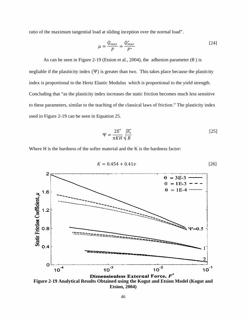
46

ratio of the maximum tangential load at sliding inception over the normal load”.

𝜇𝜇 =𝑄𝑄𝑚𝑚𝑚𝑚𝑚𝑚𝑃𝑃

=𝑄𝑄𝑚𝑚𝑚𝑚𝑚𝑚∗

𝑃𝑃∗

[24]

As can be seen in Figure 2-19 (Etsion et al., 2004), the adhesion parameter (θ ) is

negliable if the plasiticity index (Ψ) is greater than two. This takes place because the plasticity

index is proportional to the Hertz Elastic Modulus which is proportional to the yield strength.

Concluding that “as the plasticity index increases the static friction becomes much less sensitive

to these parameters, similar to the teaching of the classical laws of friction.” The plasticity index

used in Figure 2-19 can be seen in Equation 25.

Ψ =2𝐸𝐸′𝜋𝜋𝜋𝜋𝜋𝜋

�𝜎𝜎𝑠𝑠𝑅𝑅

[25]

Where H is the hardness of the softer material and the K is the hardness factor:

𝜋𝜋 = 0.454 + 0.41𝑣𝑣 [26]

Figure 2-19 Analytical Results Obtained using the Kogut and Etsion Model (Kogut and

Etsion, 2004)

47

2.3.4) Methodology of Analytical Method

To obtain any of the values needed to obtain the plasticity index and adhesion parameter,

the raw surface heights need to be gathered using a profilometer as shown in Figure 2-20. Raw

surface heights were taken of twenty samples of tin plated copper; ten samples would be placed

under the weight set and the remaining ten samples would be placed on the inclining plane.

After the raw surface heights are collected from the profilometer the program Dektak v.9 was

used to perform a first order leveling6

.

Figure 2-20 Profilometer Used to Obtain Raw Surface Data 6 Fit a function to the surface heights (in this case a linear function); use that equation to obtain calculated values. Then subtract the calculated values from the measured value. This procedure will then “flatten” the data along the x-axis. In short, to remove any slope of the sample

48

The next figure is an example of one of the first order leveling of the raw surface heights.

It can be seen that the raw surface heights are still not leveled due to the “arc” that can be seen in

Figure 2-21. Because of the “arc”, an additional second order leveling was performed; using the

best fit function, which in this case is a parabolic function7

Figure 2-21 First Order Leveling of Raw Surface Heights of Sample

. Figure 2-22 shows the second order

leveling of the same sample discussed (the other second order leveling will be displayed in

Appendix D). Figure 2-23 is the average leveled data of the ten samples that was attached under

the weight set, and Figure 2-24 is the average leveled data of the ten samples was attached to the

inclined plane.

7 The samples were cut out of a roll. So the samples were bent, despite the fact that they were cut out.

0 200 400 600 800 1000 1200 1400 1600 1800 2000-4000

-2000

0

2000

4000

6000

8000

10000

12000

Lateral distance,µm

Leve

led

Dat

a,A

m

y = 0.0024*x2 - 4*x + 8.4e+002

surface heightsparabolic

49

Figure 2-22 Second Order Leveling of Raw Surface Heights of Sample

Figure 2-23 Second Order Leveling of Raw Surface Heights of Samples that was Placed

Under the Weight Set

0 200 400 600 800 1000 1200 1400 1600 1800 2000-4000

-2000

0

2000

4000

6000

8000

10000


Leve

led D

ata,A

m

0 200 400 600 800 1000 1200 1400 1600 1800 2000-1000

-800

-600

-400

-200

0

200

400

600

800

1000


Leve

led

Dat

a,A

m

50

Figure 2-24 Second Order Leveling of Raw Surface Heights of Samples that was Placed on

the Inclined Plane

With the leveled data above, the spectral moments outlined by McCool can be found.

Spectral moments m0, m2, and m4 are the variance of heights, mean square slope, and the mean

square curvature respectively.

𝑚𝑚0 =1𝑠𝑠�𝑧𝑧2(𝑚𝑚)∞

𝑖𝑖=1

[27]

𝑚𝑚2 =1𝑠𝑠��

𝑑𝑑𝑧𝑧(𝑚𝑚)𝑑𝑑𝑚𝑚

�2∞

𝑖𝑖=1

[28]

𝑚𝑚4 =1𝑠𝑠��

𝑑𝑑2𝑧𝑧(𝑚𝑚)𝑑𝑑𝑚𝑚2 �

2∞

𝑖𝑖=1

[29]

0 200 400 600 800 1000 1200 1400 1600 1800 2000-1000

-800

-600

-400

-200

0

200

400

600

800


Levele

d D

ata

,Am

51

Spectral moments m2 and m4 can be calculated using the forward, central and backward

difference methods. From the above spectral moments, the following equations for the

asperity radius of curvature, and the asperity height standard deviation can be derived:

𝑅𝑅 = 0.375 � 𝜋𝜋𝑚𝑚4�

1 2⁄

[30]

𝜎𝜎𝑠𝑠 = �1 − 0.8968𝛼𝛼

�1 2⁄

𝑚𝑚01 2⁄ [31]

Where α is the bandwidth parameter:

𝛼𝛼 =(𝑚𝑚0𝑚𝑚4)𝑚𝑚2

2 [32]

The values obtained from Equations 27-31 and material properties obtained from other sources

were used to calculate the plasticity index and the adhesion parameter. Table 2-9 lists the

spectral moments, the asperity radius curvature, the summit height standard deviation, the

surface standard deviation, the plasticity index, and the adhesion parameter. Appendix E is the

Matlab code that is used to calculate the values shown in Table 2-9.

52

Table 2-9 Numerical Values of Parameters Parameter Units Value

𝑚𝑚0 m2 1.0721E-15

𝑚𝑚2 n/a 1.1537E-5

𝑚𝑚4 m-2 1.045E7

R m 2.0561E-4

Y N/m2 9E6

𝜎𝜎𝑠𝑠 m 3.2568E-8

C n/a 1.6485

𝐸𝐸′ Pa 2.4857E10

𝑣𝑣 n/a 0.33

Ψ n/a 15

53

CHAPTER 3- A STUDY OF VIBRATION AND THERMAL INDUCED FRETTING CORROSION

3.1 Similarities between Vibration and Thermal Cycling Models

Recently finite element models have proven to be extremely efficient and reliable. Both

2-D models were constructed in ABAQUSTM and modeled to simulate a single blade/receptacle

connector (Figure 3-1 and Figure 3-2). The geometric models for the crimp, receptacle, spring,

and supplementary mass are identical in both (vibration and thermal cycling) models. There are

differences in the other components of the models and they will be discussed further in this

chapter.

Figure 3-1 Blade/receptacle Connector Apart (Chen, 2009b)

Figure 3-2 Blade/receptacle Connector in Contact (Chen, 2009b)

Determining when fretting corrosion induces (in both models) takes place when the

horizontal distance (slip) between two specific nodes (points of contact) on the blade and

receptacle (see Figure 3-3) reaches a specified amount. “Almost any slip (>1 μm) resulted in an

54

increased contact resistance in the performed experiments” (Hammam et al., 2005). The

specified horizontal distance that was used for both of these models was 1.5μm, because that

value was used in “A Study of the Prediction of Vibration-Induced Fretting Corrosion in

Electrical Contacts” (Chen, 2009b) and “A Study of Vibration-Induced Fretting Corrosion for

Electrical Connectors” (Xie, 2006).

Figure 3-3 Displays the Output and Input Nodes as well as the Points of Contact on the Receptacle and Blade Respectively

The purpose of each finite element model is different. The vibration model, will

determine how the onset of fretting corrosion caused by vibration cycling varies under constant

temperature. The thermal cycling model, will determine how the onset of fretting corrosion is

caused by thermal cycling alone. These two models will be discussed in sections 3.2 and 3.3

respectively.

Output Node Input Node

Points of Contact

55

3.2 Vibration Model

3.2.1 Geometric Model

Figure 3-4 shows the overall view of the model and Figure 3-5 is a closer view of the

blade, crimp, receptacle, spring, and supplementary mass. The construction of this model was

based on the model that was previously constructed in ANSYSTM that was used in Chen, 2009b

and Xie, 2006. Table 3-1 displays the dimensions and density of the components in the model.

Figure 3-4 2-D ABAQUSTM Model of the Blade/Receptacle Connector

Figure 3-5 Close Up of Spring, and Receptacle of the 2-D ABAQUSTM Model of the

Blade/Receptacle Connector

Cable

Supplementary Mass

Blade

Spring

Receptacle

Crimp U-bend

56

Table 3-1 The Thickness and Density of the Components Used in the Model (Chen et al., 2009b)

Components Thickness (mm) Density (kg/m3)

Blade 1.50 8910

U-bend portion of the cantilever beam 1.90 8910

Cantilever beam spring in the receptacle 1.50 8910

Receptacle (excluding spring member) and part of

cable under the crimp

2.55 8910

Cable portion outside the crimp 1.12 4564

Supplementary mass (balls) 2.55 12876

The real thickness of the cable is not 1.12mm. Because the cable’s cross section was

modeled as a square instead of a circle an equivalent thickness was utilized. Because of the

geometric change Equation 33 (Xie, 2006) was used to come up with an equivalent thickness.

𝐼𝐼𝑒𝑒𝑞𝑞𝑒𝑒𝑖𝑖𝑣𝑣𝑚𝑚𝑙𝑙𝑒𝑒𝑠𝑠𝑖𝑖 ∗ 𝐸𝐸𝑒𝑒𝑞𝑞𝑒𝑒𝑖𝑖𝑣𝑣𝑚𝑚𝑙𝑙𝑒𝑒𝑠𝑠𝑖𝑖 = 𝐼𝐼𝑟𝑟𝑒𝑒𝑚𝑚𝑙𝑙 ∗ 𝐸𝐸𝑟𝑟𝑒𝑒𝑚𝑚𝑙𝑙 [33]

Where 𝐸𝐸 is the Young’s Modulus and I is the second moment of area. It should be noted

that the Young’s modulus for the outer structure of the receptacle (excluding the annulus

and spring inside the receptacle) was set to a very large value. The reason for that is

because the receptacle was modeled without two sides of the “hollow” box (which is

necessary so that the mechanics the spring and blade is visible). Due to the fact that the

two sides of a box was removed Young’s Modulus of the receptacle needs to be

significantly larger. With the larger Young’s Modulus, the structure would not deform as

the blade was being inserted into the receptacle. The Young’s Modulus was set to be

1000 times larger than the original value of the material used to construct the receptacle.

57

This form of tin plated copper will be entitled: rigid tin plated copper.

To ensure the geometry of the ABAQUSTM and ANSYSTM models are compatible the

transfer functions (Figure 3-6) and between frequency and the vertical amplitude (threshold

displacement at the shaker head) (Figure 3-7) both were compared and deemed compatible. For

this particular model, the transfer function is the ratio of the output node’s displacement and the

input node’s displacement. Because (both experimentally and computationally) the blade is

fixed to the shaker, the input displacement is the same as the shaker head. The transfer function

can be mathematically expressed as:

𝑇𝑇𝑟𝑟𝑚𝑚𝑠𝑠𝑠𝑠𝑓𝑓𝑒𝑒𝑟𝑟 𝐹𝐹𝑒𝑒𝑠𝑠𝜋𝜋𝑖𝑖𝑖𝑖𝐹𝐹𝑠𝑠 = 𝑀𝑀 cos𝜙𝜙 + 𝑖𝑖 𝑀𝑀 sin𝜙𝜙 [34]

Where 𝜙𝜙 is the phase angle and 𝑀𝑀 is the magnitude. Based on the transfer function the

relative motion (𝑍𝑍𝑓𝑓) can be mathematically expressed as:

𝑍𝑍𝑓𝑓 = �(1 −𝑀𝑀 cos𝜙𝜙)2 + (𝑀𝑀 sin𝜙𝜙)2 [35]

Figure 3-6 Comparison of the Transfer Functions to Show Compatibility

20 30 40 50 60 70 800.85

0.9

0.95

1

1.05

1.1

1.15

1.2

Tran

sfer

Fun

ctio

n

Frequency, Hz

ABAQUSExperimental

58

Figure 3-7 Graph to Display that the Current ABAQUSTM Model is Compatible with the Previous ANSYSTM Model and Experiment

3.2.2 Meshing and Element Type

ABAQUSTM does not consider temperature, even though the purpose of the simulation is

to determine how temperature affects fretting corrosion during vibration cycling. The element

type that is being used is the plane stress element (CPS4R) which according to ABAQUSTM is

defined as: “A 4-node bilinear plane stress quadrilateral, reduced integration, hourglass control”.

Figure 3-8 displays the mesh of the system. It can be seen that the bend of the spring has the

finest mesh, while less detailed parts of the model (such as the cable) have a coarser mesh (see

Figure 3-9); which is necessary because there is more interest in the mechanism taking place in

the connector, not the cable.

30 32 34 36 38 40 42 44 46 48 500.5

1

1.5

2

2.5

3

Thre

shol

d D

ispl

acem

ent a

t the

Sha

ker H

ead,

mm

Frequency, Hz

2-D ABAQUS2-D ANSYSExperiment

59

Figure 3-8 Displaying How ABAQUSTM Meshes the Vibration Model

Figure 3-9 How ABAQUSTM Meshes the Blade, Spring, Crimp and Receptacle

3.2.3 Material Properties

In section 3.2.3, one of the initial conditions states that the vibration cycling took place at

a specific temperature. Because of this, the Young’s Modulus of the cable8 and the friction

coefficient between the blade and the receptacle will be different at each temperature tested. The

temperature dependent Young’s Modulus for tin plated copper and a rigid tin plated copper, was

found in the ASTM Special Technical Publication No. 181 (Upthegrove et al., 1956) and for the

Silicone Rubber (which was used to calculate the Young’s Modulus of the cable9) was found in

Tran et al. 2001 (Tables 3-2, 3-3, and 3-4). The static friction coefficient was determined

experimentally (section 2.2). The constant temperatures at which vibration cycling will take

place are: 50 °C, 75 °C, and 110 °C10

8 With the information given by Upthegrove et al., 1956, the Young’s Modulus of tin plated copper and rigid tin plated copper stays the same during those temperatures

.

9 Using a form of equation 31, the combined Young’s Modulus was determined. 10 These temperatures were selected based on the availability of the needed material properties.

60

Table 3-2 List of Materials Used in Model and Corresponding Young’s Modulus and the Static Friction Coefficient at 50 °C (Upthegrove et al., 1956, Olin Brass®, and Tran et al.

2001) Material Young’s Modulus (N/m2) Static Friction Coefficient

Tin Plated Copper 129742E6 (See Table 2-5)

Rigid Tin Plated Copper 129742E9 ~

Cable 1673.95E6 ~

Table 3-3 List of Materials Used in Model and Corresponding Young’s Modulus and the

Static Friction Coefficient at 75 °C (Upthegrove et al., 1956, Olin Brass®, and Tran et al. 2001)

Material Young’s Modulus (N/m2) Static Friction Coefficient



Cable 1721.50E6 ~

Table 3-4 List of Materials Used in Model and Corresponding Young’s Modulus and the Static Friction Coefficient at 110 °C (Upthegrove et al., 1956, Olin Brass®, and Tran et al.

2001) Material Young’s Modulus (N/m2) Static Friction Coefficient



Cable 1543.73E6 ~

61

3.2.4 Boundary Conditions

The boundary conditions listed below was setup to simulate the blade/receptacle

connector undergoing vibration cycling while the surrounding temperature is set to a specific

temperature. This model undergoes three steps, which are described below.

1. Initial Conditions: Cable end is fixed. Select temperature and change material properties

accordingly (see Figure 3-10 below).

2. Step 1 (0.1 sec): Cable and receptacle are fixed; in addition to the initial conditions, a

concentrated load (see Figure 3-11) was added. The reason for the concentrated load is to

simulate contact normal force, between blade and spring (see Figure 3-11 below).

3. Step 2 (0.5 sec): Cable is still fixed; receptacle is no longer fixed. Vertical displacement

amplitudes and frequencies on blade are specified ahead of time (see Figure 3-12 below).

Figure 3-10 Visually Describing the Initial Conditions of the Model

Figure 3-11 Visually Describing the First Step of the Model

Concentrated Load

62

Figure 3-12 Visually Describing the Final Step of the Model

3.2.5 Results and Process

The change in distance between the two points of contact is caused by the vertical

displacement taking place at the outer end of the blade: because temperature is constant therefore

differential thermal expansion does not play a part. Figure 3-13 shows that in this model,

temperature does not play that large of a role. To ensure that it was not a programming error, the

Transfer Functions of the model for each temperature are shown in Figure 3-14.

Figure 3-13 Graphically Displaying How Constant Temperature Plays Apart During Vibration Cycling in this Model

30 32 34 36 38 40 42 44 46 48 500.4

0.6

0.8

1

1.2

1.4

1.6

1.8

2

Frequency, Hz

Thre

shold

Disp

lacem

ent a

t the

Sha

ker H

ead,

mm

75 C50 C110 C

63

Figure 3-14 Transfer Functions11

There are two reasons to expect these results. Because of the limited temperature range

there was not a large difference in the Young’s Modulus for each cable. Also due to the limited

temperature range, the Young’s Modulus of tin plated copper and rigid tin plated copper did not

change at all; causing even less change from temperature to temperature.

of the Connector Model at 50 °C, 75 °C, and 110 °C

11 Use equations 34 and 35

20 30 40 50 60 70 800.92

0.94

0.96

0.98

1

1.02

1.04

1.06

1.08

1.1

1.12T

rans

fer

Fun

ctio

n

Frequency, Hz

50 C75 C110 C

64

3.3 Thermal Cycling Model

3.3.1 Geometric Model

The same spring, receptacle, and crimp that were used in the model described in the

vibration model (section 3.2) was used in the thermal cycling model (see Figure 3-15 for an

overall view). The cable in the thermal cycling model does have a modification, which can be

seen in Figure 3-16. The blade also underwent some modifications as well. The reason for these

modifications will be discussed further in the following sections (3.3.2.1 and 3.3.2.2).

Figure 3-15 2-D ABAQUSTM Model Used to Simulate Thermal Cycling

Figure 3-16 Close-Up of Model Used to Simulate Thermal Cycling

Silicone Rubber Copper

65

3.3.2 Meshing and Element Type

The meshing of the thermal cycling model is very similar to that of the vibration model.

Like the vibration model, the bend of the spring has the finest mesh, while less detailed parts of

the model (such as the cable) have a coarser mesh (See Figures 3-17 and 3-18). It should be

noted that the mesh of the blade is finer in the thermal cycling model than in the vibration model.

Because differential thermal expansion is driving the motion of the model due to change of

temperature a different element type is being used. The element type that is being used for this

model is coupled temperature-displacement (CPE4RT). According the ABAQUSTM, the

definition of this type of element is: “A 4-node plane strain thermally coupled quadrilateral,

bilinear displacement and temperature, reduced integration, hourglass control.”

Figure 3-17 Displaying How ABAQUSTM Meshes the Thermal Cycling Model

Figure 3-18 How ABAQUSTM Meshes the Blade, Spring, Crimp and Receptacle

66

3.3.3 Material Properties

As was discussed in Section 3.2.2, material properties do change as a function of

temperature. All of these have either been experimentally determined and/or have been

published in tables in either handbooks or textbooks. The upcoming sections will be discussing

the following temperature dependent properties: heat transfer coefficient, thermal conductivity,

thermal expansion, Young’s Modulus, and static friction coefficient.

3.3.3.1 Heat Transfer Coefficient

According to thermophysical property tables in the back of any heat transfer textbook

various properties of gases that affect the heat transfer coefficient such as kinematic viscosity,

conductivity, and Prandtl Number, are tabulated as a function of temperature. Using the values

found in the appendix (A.4) of “Fundamentals of Heat and Mass Transfer” by Incropera et al.,

the following equation (derived by Churchill and Bernstein) could be used for the blade,

receptacle, and the cable:

𝜇𝜇𝑒𝑒𝐷𝐷�� =ℎ�𝐷𝐷𝜋𝜋

= 0.3 +0.62𝑅𝑅𝑒𝑒𝐷𝐷

1 2⁄ 𝑃𝑃𝑟𝑟1 3⁄

[1 + (0.4 𝑃𝑃𝑟𝑟⁄ )2 3⁄ ]1 4⁄ �1 + �𝑅𝑅𝑒𝑒𝐷𝐷

282,000�5 8⁄

�4 5⁄

[36]

It should be noted that the cable is not modeled as a cylinder, but as a rectangular cube (Section

3.2.1). Therefore the equation used to find the heat transfer coefficient would be the same as the

one used for the other rectangles in the model. In order to use equation 36 to find ℎ�, some key

assumptions were made :

1. The velocity of the air (𝑈𝑈∞) as it passes over the connector is 0.76 m/s, which is the

velocity of the air inside a temperature chamber.

2. Convection is only being applied in one direction (see Figure 3-19)

67

3. The type of convection being used is forced convection. This is the only type of

convection that can be used in ABAQUSTM (Analysis User Manuel Volume V).

4. The temperature used to determine the properties, which would determine the heat

transfer coefficient, is the surrounding temperature. There are two reasons to use the

surrounding temperature instead of the film temperature (average of the surface and the

surroundings):

• Initial temperatures of both the surroundings and the surfaces are the same (room

temperature).

• Convection alone is heating the model (there is no electrical current going through

the model).

The validity of assumption number four comes from what happens physically to the model

(which is discussed in the two bullets above). The difference between the film temperature, the

temperatures of the surroundings and the surface temperature would be negligible. Figure 3-19

displays how each part of the connector was modeled, displaying the characteristic length used to

calculate the Reynolds Number. Tables 3-5, 3-6, and 3-7 display the Heat Transfer coefficient

values calculated by equation 36 and entered into ABAQUSTM. Also in Figure 3-20 shows how

the blade was modified to ensure that convection would not be taking place inside of the

receptacle.

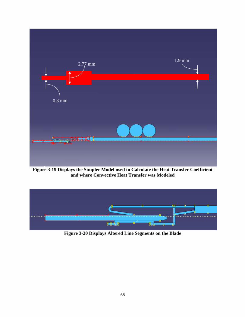
68

Figure 3-19 Displays the Simpler Model used to Calculate the Heat Transfer Coefficient

and where Convective Heat Transfer was Modeled

Figure 3-20 Displays Altered Line Segments on the Blade

2.77 mm

0.8 mm

1.9 mm

69

Table 3-5 Temperature Dependent Heat Transfer Coefficient for the Receptacle Temperature (°C) Heat Transfer Coefficient (W/m2-°C)

-173.15 1.07

-123.15 1.55

-73.15 2.01

26.85 2.90

76.85 3.30

126.85 3.71

226.85 4.46

326.85 5.13

476.85 6.00

826.85 7.79

926.85 8.31

1226.85 10.88

1826.85 15.98

2226.85 24.11

2726.85 52.76

70

Table 3-6 Temperature Dependent Heat Transfer Coefficient for the Blade Temperature (°C) Heat Transfer Coefficient (W/m2-°C)

-173.15 3.61

-123.15 5.28

-73.15 6.89

26.85 9.96

76.85 11.35

126.85 12.77

226.85 15.36

326.85 17.68

476.85 20.68

826.85 26.90

926.85 28.70

1226.85 37.60

1826.85 55.22

2226.85 83.38

2726.85 182.47

71

Table 3-7 Temperature Dependent Heat Transfer Coefficient for the Cable Temperature (°C) Heat Transfer Coefficient (W/m2-°C)

-173.15 1.54

-123.15 2.24

-73.15 2.92

26.85 4.22

76.85 4.80

126.85 5.40

226.85 6.49

326.85 7.47

476.85 9.11

826.85 11.35

926.85 12.11

1226.85 15.85

1826.85 23.28

2226.85 35.14

2726.85 76.88

72

3.3.3.2 Thermal Conductivity and Thermal Expansion

In order to obtain an accurate response from the cable during thermal cycling, two

sections had to be added to the cable (see Figure 3-16). As can be seen from Tables F-3 and F-4,

the difference between the thermal expansions of both copper and silicone rubber is extremely

large. Also combining the two of them together would be inaccurate, because area for the

copper and silicone rubber are not equal to each other. Because of that reason, picking either one

of the material’s thermal expansions is not an option. In order to obtain an accurate temperature

distribution using separate thermal conductivities was necessary. It can be seen on Table F-1 and

F-2 that the thermal conductivities of both materials are very different:

3.3.3.3 Young’s Modulus

In Section 3.3.1, it is stated that the Young’s Modulus of the outer structure (rigid tin

plated copper) of the receptacle is set to a very large value (numerical values used in the program

can be seen in Table F-8). To determine how Young’s Modulus varies with temperature, the

values determined for tin plated copper was scaled12

3.3.3.4 Static Friction Coefficient

for rigid tin plated copper. The Young’s

Modulus for the components of the cable (silicone rubber and copper) are also listed in Tables F-

9 and F-10.

The static friction coefficient for tin on tin was experimentally found using methods

discussed in Chapter 2. Tables 2-6, 2-7, and 2-8 display the numerical values that were

graphically displayed in Chapter 2 (see Figures 2-11 to 2-16). Because the pressure between the

spring and the blade was extremely high (due to a small contact area), the static friction

12 1000x greater

73

coefficient was determined at several pressures. ABAQUSTM will be able to determine a

function, thus determining the static friction coefficient at the specified temperature and pressure.

3.3.4 Boundary Conditions

The boundary conditions listed were setup to simulate the blade/receptacle connector

undergoing thermal cycling. This model undergoes three steps which are described in the steps

below.

1. Initial Conditions: Receptacle, blade, and cable are all fixed. Room temperature (20 °C)

is the initial temperature (see Figure 3-21).

2. Step 1 (0.1 sec): Same as initial conditions; in addition to the initial conditions a

concentrated load was added. The concentrated load simulates contact normal force,

between blade and spring (see Figure 3-22).

3. Step 2: Blade and cable are still fixed, receptacle is no longer fixed. Temperature

amplitudes and frequencies are specified (See Figure 3-19).

Figure 3-21 Visually Describing the Initial Conditions of the Model

Figure 3-22 Visually Describing the First Step of the Model

Concentrated Load

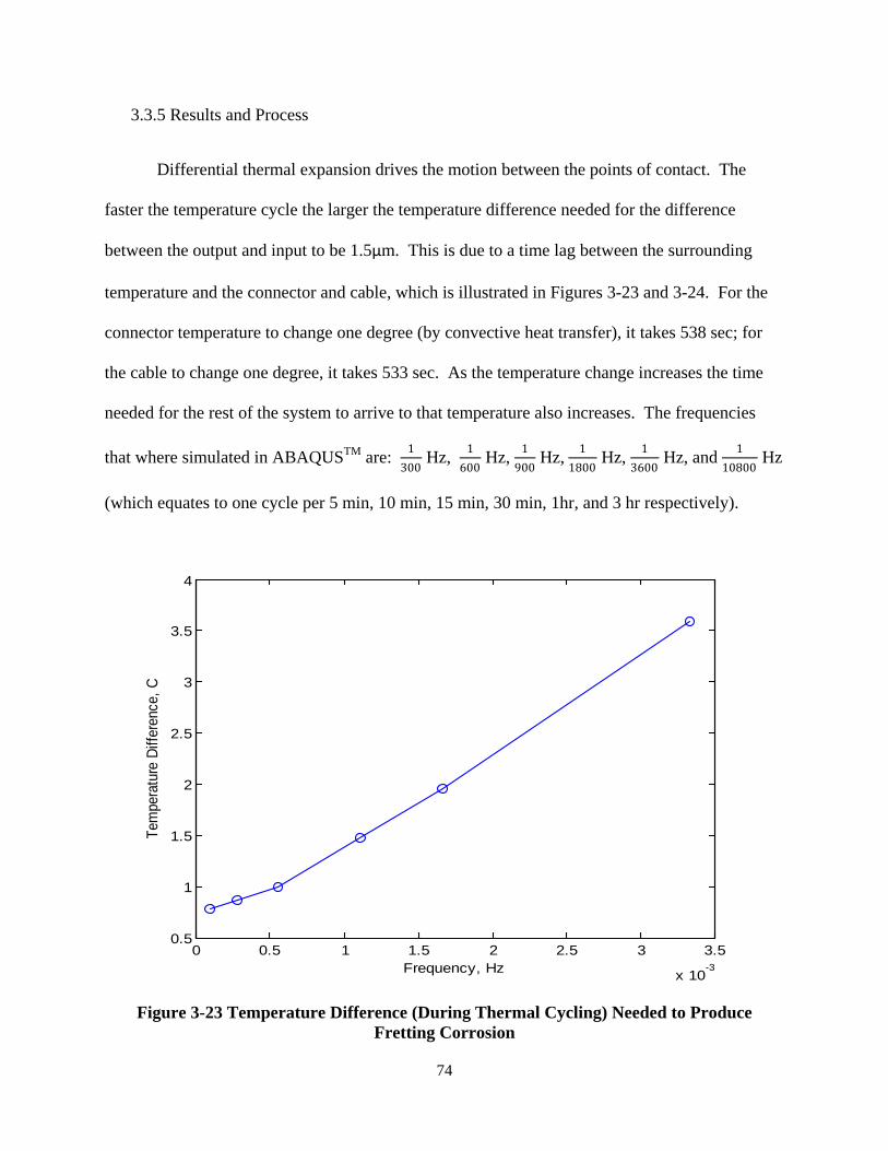
74

3.3.5 Results and Process

Differential thermal expansion drives the motion between the points of contact. The

faster the temperature cycle the larger the temperature difference needed for the difference

between the output and input to be 1.5μm. This is due to a time lag between the surrounding

temperature and the connector and cable, which is illustrated in Figures 3-23 and 3-24. For the

connector temperature to change one degree (by convective heat transfer), it takes 538 sec; for

the cable to change one degree, it takes 533 sec. As the temperature change increases the time

needed for the rest of the system to arrive to that temperature also increases. The frequencies

that where simulated in ABAQUSTM are: 1300

Hz, 1600

Hz, 1900

Hz, 11800

Hz, 13600

Hz, and 110800

Hz

(which equates to one cycle per 5 min, 10 min, 15 min, 30 min, 1hr, and 3 hr respectively).

Figure 3-23 Temperature Difference (During Thermal Cycling) Needed to Produce Fretting Corrosion

0 0.5 1 1.5 2 2.5 3 3.5

x 10-3

0.5

1

1.5

2

2.5

3

3.5

4

Frequency, Hz

Tem

pera

ture

Diff

eren

ce, C

75

Figure 3-24 Time Lag Between Cable Temperature and Surrounding Temperature at

Various Temperature Differences

Figure 3-25 Time Lag Between Connector Temperature and Surrounding Temperature at

Various Temperature Differences

0 200 400 600 800 1000 1200 1400 1600 1800 2000

-25

-20

-15

-10

-5

0

5

10

15

20

25

Time, sec

Temp

eratur

e Diffe

rence

, C

Surrounding Temp. Diff., +/- 1 CCable Temp. Diff, +/- 1 CSurrounding Temp. Diff, +/- 10 CCable Temp. Diff, +/- 10 CSurrounding Temp. Diff, +/- 25 CCable Temp. Diff, +/- 25 C

0 200 400 600 800 1000 1200 1400 1600 1800 2000

-25

-20

-15

-10

-5

0

5

10

15

20

25

Time, sec

Temp

eratur

e Diffe

rence

, C

Surrounding Temp. Diff., +/- 1 CConnector Temp. Diff., +/- 1 CSurrounding Temp. Diff., +/- 10 CConnector Temp. Diff., +/- 10 CSurrounding Temp. Diff., +/- 25 CConnector Temp. Diff., +/- 25 C

76

CHAPTER 4- CONCLUSION AND FUTURE WORK

Two experiments and two computational models have been presented in this thesis. Both

experiments examined how pressure and temperature affect the static friction coefficient. It was

found that as the pressure increased the static friction coefficient decreased. This held true to the

previously published data (Cohen et al. 2008). Because trend of the analytical and the

experimental data coincided, data produced from that apparatus could be trusted. That same

apparatus was then used in a temperature chamber to see how temperature affected the static

friction coefficient. It was found that as temperature increased the static friction coefficient

decreased. This was expected, so the results obtained from that experiment were then entered

into the finite element models.

With the data from the experiments conducted in the previous paragraph and other

experiments done in the past, both finite element models were constructed and produced results.

In the vibration model, because the material properties varied very little it was hardly any

change, but it can be seen that the same overall trend (as the frequency increases, the threshold

displacement at the shaker head, decreases) obtained from that program matches the trend from

Chen, 2009b. The second model showed how thermal cycling affects fretting corrosion. The

results obtained from that model show that as the frequency of the temperature increases the

higher the temperature amplitude (difference) needed for fretting corrosion to start. The reason

for this is due to the time lag between the surrounding temperature and the temperature of the

connector and the cable.

77

Progress has been made in the field of fretting corrosion, but more can be done. The

following are some suggestions for future research in this area:

• Create a finite element model that not only includes vibration and thermal cycling, but

also include electrical current. Electrical current would be a practical and interesting

parameter.

• Create a 3-D model to simulate how thermal cycling affects fretting corrosion.

• Design an experiment that can either confirm or reject the 2-D and 3-D finite element

models.

• Expand the temperature range in which the temperature dependent materials are tested.

Many of the properties are tested at room temperature and above; material properties that

were tested at temperatures below room temperature are few and far between.

• Retesting the temperature dependent material properties that would be entered in a finite

element model. The vast majority of the temperature dependent properties, for materials

used in connectors, were tested in 1950-1970’s. Experimental measurements have since

greatly improved.

78

References

[1] S.V. Angadi, W.E. Wilson, R.L. Jackson, G.T. Flowers, and B.I. Rickett, "A multi-physics

finite element model of an electrical connector considering rough surface contact," IEEE

Trans. CHMT, 2008, pp. 168-177.

[2] M. Antler, "Survey of Contact Fretting in Electrical Connectors," IEEE Trans. CHMT, vol. 8,

1985, pp. 87-104.

[3] P.J. Arrazola and T. Ozel, "Investigations on the effects of friction modeling in finite element

simulation of machining," International Journal of Mechanical Sciences, vol. 52, 2010, pp.

31-42.

[4] M. Attia, Standardization of Fretting Fatigue Test Methods and Equipment, Philadelphia,

PA: ASTM Publication Code, 1992.

[5] E.M. Bock and J.H. Whitley, "Fretting corrosion in electric contacts," IEEE Holm Conf,

1974, pp. 128-138.

[6] J.C. Bowling, 2007 Baccalaurate Sermon, Bourbonnais: 2007.

[7] W. Chang, I. Etsion, and D. Bogy, "Static Friction Coefficient Model for Metallic Rough

Surfaces," ASME Journal of Tribology, vol. 110, 1988, pp. 57-63.

[8] C. Chen, "A Study of the Prediction of Vibration-Induced Fretting Corrosion in Electrical

Contacts," 2009.

[9] D. Cohen, Y. Kligerman, and I. Etsion, "A Model for Contact and Static Friction of

Nominally Flat Rough Surfaces Under Full Stick Contact Condition," ASME Journal of

Tribology, vol. 130, 2008, pp. 1-9.

[10] J. Davis, Metals Handbook, Materials Park, OH: ASM International, 1998.

79

[11] J. Dunkin and D. Kim, "Measurement of Static Friction Coefficient Between Flat Surfaces,"

Wear, vol. 193, 1996, pp. 186-192.

[12] I. Etsion, "A Model for Static Sealing Performance of End Face Seals," STLE Tribology

Transactions, vol. 37, 1994, pp. 111-119.

[13] I. Etsion and I. Front, "Model for Static Sealing Performance of End Face Seals," STLE

Tribology Transactions, vol. 37, 1994, pp. 111-119.

[14] G.T. Flowers, F. Xie, M.J. Bozack, X. Hai, B.I. Rickett, and R.D. Malucci, "A Study of the

Physical Characteristics of Vibration-Induced Fretting Corrosion," IEEE Trans. CHMT, vol.

29, 2006, pp. 318-325.

[15] G.T. Flowers, F. Xie, M.J. Bozack, and R.D. Malucci, "Vibration Thresholds for Fretting

Corrosion in Electrical Connectors," IEEE Trans. CHMT, vol. 27, 2004, pp. 65-71.

[16] M. Fontana, Corrosion Engineering, New York, New York: McGraw Hill, 1986.

[17] H. Gao and G.C. Barber, "Microcontact Model for Paper-Based Wet Friction Materials,"

ASME Journal of Tribology, vol. 124, 2002, pp. 414-419.

[18] J. Geringer, B. Forest, and P. Combrade, "Fretting-corrosion of materials used as

orthopaedic implants," Wear, vol. 259, 2005, pp. 943-951.

[19] J. Greenwood and J. Williamson, "Contact of Nominally Flat Surfaces," Royal Society of

London. Series A. Mathematical and Physical Sciences, 1966, pp. 300-319.

[20] Incropera, DeWitt, Bergman, and Lavine, Fundamentals of Heat and Mass Transfer,

Hoboken, NJ: Wiley and Sons, .

[21] M. Karamis and B. Selcuk, "Analysis of the Friction Behavior of Bolted Joints," Wear, vol.

166, 1993, pp. 73-83.

80

[22] L. Kogut and I. Etsion, "A Static Friction Model for Elastic- Plastic Contacting Rough

Surfaces," ASME Journal of Tribology, vol. 126, 2004, pp. 34-40.

[23] H. Kongsjorden, J. Kulset, and J. Sletbak, "Degradation of Electrical Contacts Caused by

Oscillatory Micromotion Between the Contact Members," IEEE Trans. CHMT, vol. 2, 1979,

pp. 32-36.

[24] A. Lee and M.S. Mamrick, "Fretting Corrosion of Tin-Plated Copper Alloy," IEEE Trans.

CHMT, 1987, pp. 63-67.

[25] A. Lee and M.S. Mamrick, "Fretting corrosion of tin at elevated temperatures," IEEE Trans.

CHMT, 1988, pp. 87-91.

[26] G.H. Majzoobi, J. Nemati, A.J. Rooz, and G.H. Farrahi, "Modification of fretting fatigue

behavior of AL7075–T6 alloy by the application of titanium coating using IBED technique

and shot peening," Tribology International, vol. 42, 2009, pp. 121- 129.

[27] R.D. Malucci, "Accelerated Testing of Tin-Plated Copper Alloy Contacts," IEEE Trans.

CHMT, vol. 22, 1999, pp. 53-60.

[28] R.D. Malucci, "Impact of fretting parameters on contact degradation," IEEE Trans. CHMT,

1996, pp. 395-403.

[29] J.W. McBride, "Developments in fretting studies applied to electrical contacts," Institute of

Electrical and Electronics Engineering, 2006, pp. 170-180.

[30] J. McCool, "Relating Profile Instrument Measurements to the Functional Performance of

Rough Surfaces," ASME Journal of Tribology, vol. 109, 1987, pp. 264-270.

[31] A. Monnier, B. Froidurot, C. Jarrige, and R. Meyer, "A Mechanical, Electrical, Thermal

Coupled-Field Simulation of a Sphere-Plane Electrical Contact," IEEE Trans. CHMT, vol.

30, 2007, pp. 787-795.

81

[32] A. Moufki, A. Devillez, D. Dudzinski, and A. Molinari, "Thermomechanical modelling of

oblique cutting and experimental validation," International Journal, vol. 44, 2004, pp. 971-

989.

[33] A. Moufki, A. Molinari, and D. Dudzinski, "Modelling of orthogonal cutting with a

temperature dependent friction law," Journal of the Mechanics and Physics of Solids, vol.

46, 1998, pp. 2103-2138.

[34] A. Nayebi, G. Mauvoisin, and H. Vaghefpour, "Modeling of twist drills wear by a

temperature-dependent friction law," Journal of Materials Processing Technology, vol. 7,

2007, pp. 98-106.

[35] T. Ozel, "The influence of friction models on finite element simulations of machining ¨,"

International Journal of Machine Tools and Manufacture, vol. 46, 2006, pp. 518-530.

[36] Y.W. Park, T.S. Narayanan, and K.Y. Lee, "Effect of temperature on the fretting corrosion

of tin plated copper alloy contacts," Wear, vol. 262, 2007, pp. 320-330.

[37] Y.W. Park, T.S. Narayanan, and K.Y. Lee, "Fretting corrosion of tin-plated contacts,"

Tribology International, vol. 41, 2008, pp. 616-628.

[38] C. Richard, "On the Identification and Haptic Display of Friction," 2000.

[39] Y. Sang, M. Dube, and M. Grant, "Dependence of friction on roughness, velocity, and

temperature 1," Physical Review E, vol. 77, 2008, pp. 1-11.

[40] R. Serway and J. Jewett, Physics for Scientists and Engineers with Modern Physics,

Belmont, CA: Thomson, Brooks, and Cole, 2004.

[41] D. Tabor, "Friction- The Present State of Our Understanding," ASME Journal of Tribology,

vol. 103, 1981, pp. 169-179.

82

[42] D. Thuresson, "Stability of sliding contact—Comparison of a pin and a finite element

model," Wear, vol. 261, 2006, pp. 896-904.

[43] Y.S. Touloukian, Thermophysical properties of matter, New York: IFI/Plenum, 1970.

[44] D. Tran, M. Cooke, and P. Newsome, "Laboratory evaluation of mouthguard material,"

Dental Traumatology, vol. 17, 2001, pp. 260-265.

[45] C. Upthegrove and H. Burghoff, Elevated-temperature properties of coppers and

copperbase alloys. Data compiled by and issued under the auspices of the Data and

Publications Panel of the ASTM-ASME Joint Committee on Effect of Temperature on the

Properties of Metals, Philadelphia, PA: ASTM, 1956.

[46] J. Vance, Rotordynamics of turbomachinery, New York, New York: Wiley and Sons, 1988.

[47] G. Villeneuve, D. Kulkarni, P. Bastnagel, D. Berry, and W. Lafayette, "Dynamic finite

element analysis simulation of the terminal crimping process," IEEE Holm Conf, 1996, pp.

156-172.

[48] R. Waterhouse, Fretting Corrosion, New York, New York: Pergamon Press, 1972.

[49] J. Williams, Engineering Tribology, New York, New York: Cambridge University Press,

2005.

[50] F. Xie, "A study of vibration-induced fretting corrosion for electrical connectors,"

Computer, 2006.

[51] F. Xie, G.T. Flowers, C. Chen, M. Bozack, J. Suhling, B.I. Rickett, R.D. Malucci, and C.

Manlapaz, "Analysis and Prediction of Vibration-Induced Fretting Motion in a

Blade/Receptacle Connector Pair," IEEE Trans. CHMT, vol. 32, 2009, pp. 583-590.

83

[52] W. Xie, DeMeter, and M. Tretheway, "An Experimental Evaluation of Coefficients of Static

Friction of Common Workpiece-Fixture," International Journal of Machine Tools and

Manufacture, 2000, pp. 467-488.

[53] "OC Oerlikon Corporation AG, Pfäffikon - Oerlikon Solar, Oerlikon Coating, Oerlikon

Vacuum, Oerlikon Textile, Oerlikon Drive Systems, Oerlikon Components."

[54] "KSC Corrosion Technology Laboratory Home."

[55] "Bible," Psalms 3:3.

[56] "Operating Manual Digital Thermometer," 2009.

[57] "Weights of Classes E1 E2, F1, F2, M1, M1-2, M2, M2-3, Part 1: Metrological and

Technical Requirements," 2004, p. 12.

84

Appendix A- Mechanical Drawings

Figure A-1 Motorized Incline Plane

Figure A-2 Holder

Figure A-3 Leg

Figure A-4 Incline Plane

Figure A-5 Plate

Figure A-6 Rod

Figure A-7 Sensor Holder

Figure A-8 O-ring

93

Appendix B- Electrical Drawing:

Figure B-1 Electrical Drawing of Motorized Inclined Plane

94

Appendix C- Uncertainty of Experiment

The instrument uncertainties of the experiments discussed in Chapter 2 are associated

with the angle meter, the weight set, and the thermometer which will be discussed for each one

below.

The angle meter has an uncertainty of ±0.05°, which is the smallest fraction it indicates.

The additional uncertainty is caused by the position of the angle meter (Figure C-1). The angle

meter was equipped with a level (Figure C-2), which was used to make sure that one of the arms

is parallel with the base. Using the geometric theorem that states: if two parallel lines are cut by

a transverse line the alternate interior angles (caused by that line) are equal (Figure C-3); where

the angle meter (the arm with the level) and the base are parallel lines, and the inclined plane and

the other arm of the angle meter are intersecting those lines. Because the “bubble” in the level

could not be perfectly centered; in fact there are two bounds, one lower bound (Figure C-4) and

one upper bound (Figure C-5). The additional uncertainty caused by the position of the angle

meter was found to be ±0.5°. Therefore the total uncertainty of the angle meter is ±0.55°.

Taking that value (±0.55°) and entering it into equation 12 the uncertainty of the static friction

coefficient is ±0.0096.

95

Figure C-1 Measuring theta

Figure C-2 Upper View of Level

96

Figure C-3 Visual Display of Geometric Theorem Stating

Figure C-4 Lower Bound of the Level

Figure C-5 High Bound of the Level

The specifications of the weight set state that the standard used was the International

Organization of Legal Metrology M2 tolerance. According to those standards (Weights of

Classes E1 E2, F1, F2, M1, M1-2, M2, M2-3, and M3, 2004), the uncertainty for 10 g, 20 g, and 50 g

are ±6 mg, ±8 mg, and ±10 mg respectively. The masses listed in Table C-1 (which also display

Inclined Plane

Base

Angle Meter

θ

θ

97

the uncertainty) were compiled using various combinations of the masses listed in the previous

sentence.

Table C-1 Uncertainty at Each Mass Tested Mass (g) Uncertainty (±mg)

70 18

100 32

130 42

160 56

190 66

220 80

According to the operating manual of the thermometer (which also came with a K-type

thermocouple) the accuracy of the meter is ± (0.3% of the reading+2 °C). Because the

temperature chamber door, had to be opened in order for the weight set (with sample adhered to

it) to be placed on the inclined plane, the temperature changed. The temperature difference for

each temperature is in Table C-2. The upper and lower bounds can be found and is listed in

Table C-3.

98

Table C-2 Temperature Drop as Door Opens at each Temperature Desired Temperature (°C) Temperature Drop (°C)

-10 +3

10 +2

25 0

50 -2

75 -5

110 -10

Table C-3 Upper and Lower Bounds of the Temperature (including Temperature Drop) Desired Temperature (°C) Upper Bound (°C) Lower Bound (°C)

-10 -5 -9

10 14 10

25 27 23

50 50 46

75 72 68

110 102 98

99

Appendix D- Second Order Normalization of all of the Samples

D-1 Second Order Normalization of Small Sample 1

0 200 400 600 800 1000 1200 1400 1600 1800 2000-4000

-2000

0

2000

4000

6000

8000

10000

Lateral Distance (µm)

Leve

led

Dat

a (A

m)

100



0 200 400 600 800 1000 1200 1400 1600 1800 2000-3000

-2000

-1000

0

1000

2000

3000


Leve

led

Dat

a (A

m)

0 200 400 600 800 1000 1200 1400 1600 1800 2000-3000

-2000

-1000

0

1000

2000

3000


Leve

led

Dat

a (A

m)

101



0 200 400 600 800 1000 1200 1400 1600 1800 2000-6000

-4000

-2000

0

2000

4000

6000


Leve

led

Dat

a (A

m)

0 200 400 600 800 1000 1200 1400 1600 1800 2000-2000

-1500

-1000

-500

0

500

1000

1500

2000

2500


Leve

led

Dat

a (A

m)

102



0 200 400 600 800 1000 1200 1400 1600 1800 2000-5000

-4000

-3000

-2000

-1000

0

1000

2000

3000


Leve

led

Dat

a (A

m)

0 200 400 600 800 1000 1200 1400 1600 1800 2000-4000

-3000

-2000

-1000

0

1000

2000

3000


Leve

led

Dat

a (A

m)

103



0 200 400 600 800 1000 1200 1400 1600 1800 2000-1500

-1000

-500

0

500

1000

1500

2000

2500


Leve

led

Dat

a (A

m)

0 200 400 600 800 1000 1200 1400 1600 1800 2000-5000

-4000

-3000

-2000

-1000

0

1000

2000


Leve

led

Dat

a (A

m)

104


D-11 Second Order Normalization of Large Sample 1

0 200 400 600 800 1000 1200 1400 1600 1800 2000-1500

-1000

-500

0

500

1000

1500

2000

2500

3000


Leve

led

Dat

a (A

m)

0 200 400 600 800 1000 1200 1400 1600 1800 2000-2000

-1000

0

1000

2000

3000

4000


Leve

led

Dat

a (A

m)

105



0 200 400 600 800 1000 1200 1400 1600 1800 2000-5000

-4000

-3000

-2000

-1000

0

1000

2000


Leve

led

Dat

a (A

m)

0 200 400 600 800 1000 1200 1400 1600 1800 2000-4000

-3000

-2000

-1000

0

1000

2000

3000


Leve

led

Dat

a (A

m)

106



0 200 400 600 800 1000 1200 1400 1600 1800 2000-1500

-1000

-500

0

500

1000

1500


Leve

led

Dat

a (A

m)

0 200 400 600 800 1000 1200 1400 1600 1800 2000-6000

-5000

-4000

-3000

-2000

-1000

0

1000

2000

3000

4000


Leve

led

Dat

a (A

m)

107



0 200 400 600 800 1000 1200 1400 1600 1800 2000-4000

-3000

-2000

-1000

0

1000

2000


Leve

led

Dat

a (A

m)

0 200 400 600 800 1000 1200 1400 1600 1800 2000-5000

-4000

-3000

-2000

-1000

0

1000

2000

3000

4000

5000


Leve

led

Dat

a (A

m)

108



0 200 400 600 800 1000 1200 1400 1600 1800 2000-4000

-3000

-2000

-1000

0

1000

2000

3000

4000

5000


Leve

led

Dat

a (A

m)

0 200 400 600 800 1000 1200 1400 1600 1800 2000-3000

-2000

-1000

0

1000

2000

3000


Leve

led

Dat

a (A

m)

109


0 200 400 600 800 1000 1200 1400 1600 1800 2000-5000

-4000

-3000

-2000

-1000

0

1000

2000


Leve

led

Dat

a (A

m)

110

Appendix E- Matlab Code Used to Find Plasticity Index

%zl= Profile Heights of the Average of all ten % Large Samples %zu= Profile Heights of the Average of all ten % Small Samples %Spectral Moment m_0-lower for i=1:1:n fl(i)=(zl(i)^2); end m_0l=sum(fl)/n; %Spectral Moment m_0-upper for i=1:1:n fu(i)=(zu(i)^2); end m_0u=sum(fu)/n; m_0=(m_0l)+(m_0u); %Spectral Moment m_2-lower for i=1:1:n if i==1 %Using forward difference approximation for the first data point sl(i)=((zl(i+1)-zl(i))./(x(i+1)-x(i))).^2; elseif i==3900 %Using backward difference approximation for the last data point sl(i)=((zl(i)-zl(i-1))./(x(i)-x(i-1))).^2; else %Using centered difference approximation for the rest of the data %points sl(i)=((zl(i+1)-zl(i-1))./(x(i+1)-x(i-1))).^2; end end m_2l=sum(sl)/n; %Spectral Moment m_2-upper for i=1:1:n if i==1 %Using forward difference approximation for the first data point su(i)=((zu(i+1)-zu(i))./(x(i+1)-x(i))).^2; elseif i==3900

111

%Using backward difference approximation for the last data point su(i)=((zu(i)-zu(i-1))./(x(i)-x(i-1))).^2; else %Using centered difference approximation for the rest of the data %points su(i)=((zu(i+1)-zu(i-1))./(x(i+1)-x(i-1))).^2; end end m_2u=sum(su)/n; m_2=(m_2u)+(m_2l); %Spectral Moment m_4-lower for i=1:1:n if i==1 %Using forward difference approximation for the first data point hl(i)=((zl(i+2)-(zl(i+1).*2)+zl(i))./((x(i+2)-x(i+1))*(x(i+1)-x(i)))).^2; elseif i==3900 %Using backward difference approximation for the first data point hl(i)=((zl(i)-(zl(i-1).*2)+zl(i-2))./((x(i-1)-x(i-2))*(x(i)-x(i-1)))).^2; else %Using centered difference approximation for the rest of the data %points hl(i)=((zl(i+1)-(zl(i).*2)+zl(i-1))./((x(i)-x(i-1))*(x(i+1)-x(i)))).^2; end end m_4l=sum(hl)/n; %Spectral Moment m_4-upper for i=1:1:n if i==1 %Using forward difference approximation for the first data point hu(i)=((zu(i+2)-(zu(i+1).*2)+zu(i))./((x(i+2)-x(i+1))*(x(i+1)-x(i)))).^2; elseif i==3900 %Using backward difference approximation for the first data point

112

hu(i)=((zu(i)-(zu(i-1).*2)+zu(i-2))./((x(i-1)-x(i-2))*(x(i)-x(i-1)))).^2; else %Using centered difference approximation for the rest of the data %points hu(i)=((zu(i+1)-(zu(i).*2)+zu(i-1))./((x(i)-x(i-1))*(x(i+1)-x(i)))).^2; end end m_4u=sum(hu)/n; m_4=(m_4u)+(m_4l); %Radius of Curvature R=0.375*sqrt(pi/m_4) %Bandwidth Paramenter alpha=(m_0*m_4)/((m_2)^2); %Asperity height standard deviation sigma=sqrt(1-(0.8968/alpha))*sqrt(m_0) %Material properties of tin(Metals Handbook edited by J.R Davis) Y=9*(10^6); %Yield Strength (N/m^2) v=0.33; %Poisson's Ratio E=44.3*(10^9); % Young's Modulus (N/m^2) %Hertz Modulus of Elasicity bE1=(2*(1-(v.^2)))/E; bE=1/bE1 %Function of Poission's Ratio C=1.234+(1.256*v); %Contact area: A=(17*(10^-3))^2; % (m^2) %Plasticity index Pl=sqrt(sigma/R)*((2*bE)/(C*(1-(v^2))*pi*Y))

113

Appendix F- Temperature Dependent Material Properties Table F-1 Temperature Dependent Thermal Conductivity of Tin Plated Copper and Rigid

Tin Plated Copper (Touloukian et. al, 1970 and www.matweb.com) Temperature (°C) Thermal Conductivity (W/m-°C)

20 160

56.2 164

119 181

201.2 203

316.2 223

422.2 277

500.7 256

Table F-2 Temperature Dependent Thermal Expansion of Tin Plated Copper and Rigid

Tin Plated Copper (Touloukian et. al, 1970 and www.matweb.com) Temperature (°C) Thermal Expansion (1/°C)

20 1.63E-5

127 1.67E-5

227 1.78E-5

327 1.87E-5

427 1.95E-5

527 2.09E-5

627 2.13E-5

727 2.16E-5

http://www.matweb.com/�


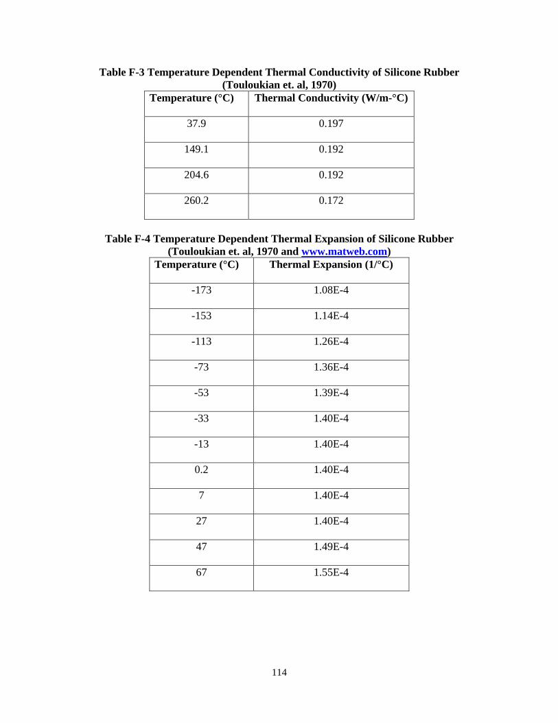
114

Table F-3 Temperature Dependent Thermal Conductivity of Silicone Rubber (Touloukian et. al, 1970)

Temperature (°C) Thermal Conductivity (W/m-°C)

37.9 0.197

149.1 0.192

204.6 0.192

260.2 0.172

Table F-4 Temperature Dependent Thermal Expansion of Silicone Rubber

(Touloukian et. al, 1970 and www.matweb.com) Temperature (°C) Thermal Expansion (1/°C)

-173 1.08E-4

-153 1.14E-4

-113 1.26E-4

-73 1.36E-4

-53 1.39E-4

-33 1.40E-4

-13 1.40E-4

0.2 1.40E-4

7 1.40E-4

27 1.40E-4

47 1.49E-4

67 1.55E-4


115

Table F-5 Temperature Dependent Thermal Conductivity of Copper (Touloukian et. al, 1970 and www.matweb.com)

Temperature (°C) Thermal Conductivity (W/m-°C)

-173 483

0 401

20 385

27 398

Table F-6 Temperature Dependent Thermal Expansion of Copper

(Touloukian et. al, 1970 and www.matweb.com) Temperature (°C) Thermal Expansion (1/°C)

20 1.64E-5

100 1.64E-5

250 1.85E-5

500 2.02E-5

925 2.48E-5

Table F-7 Temperature Dependent Young’s Modulus of Tin Plated Copper

(Upthegrove et al., 1956 and Olin Brass®) Temperature (°C) Young’s Modulus (N/m2)

20 1.297E11

23.89 1.180E11

148.89 1.180E11

204.44 1.042E11

260 1.042E11



116

Table F-8 Temperature Dependent Young’s Modulus of Rigid Tin Plated Copper (Upthegrove et al., 1956 and Olin Brass®)

Temperature (°C) Young’s Modulus (N/m2)

20 1.297E13

23.89 1.273E13

148.89 1.273E13

204.44 1.272E13

260 1.272E13

Table F-9 Temperature Dependent Young’s Modulus of Silicone Rubber

(Tran et al. 2001) Temperature (°C) Young’s Modulus (N/m2)

20 7.00E5

50 6.70E5

60 6.80E5

71 6.30E5

81 6.70E5

96 6.20E5

120 4.30E5

150 1.10E5

117

Table F-10 Temperature Dependent Young’s Modulus of Copper (Upthegrove et al., 1956 and www.matweb.com)

Temperature (°C) Young’s Modulus (N/m2)

-196.11 1.238E11

-67.78 1.272E11

-40 1.155E11

20 1.2E11

23.89 6.792E10

100 6.792E10

204.44 1.038E11


118

Appendix G- Input File for Vibration Model

** ** PARTS ** *Part, name=Ball_2D *Element, type=CPS4R ** Section: Ball_2D *Solid Section, elset=_PickedSet6, material=Ball 2.55, *End Part ** *Part, name=Blade_2D *Element, type=CPS4R ** Section: Blade_2D *Solid Section, elset=_PickedSet6, material=Star 1.5 *End Part ** *Part, name=Receptacle_part_2D *Element, type=CPS4R ** Section: Receptacle_nonrigid *Solid Section, elset=_PickedSet45, material=Star 2.55, ** Section: Receptacle_rigid *Solid Section, elset=_PickedSet44, material=Star_rigid 2.55, *End Part ** *Part, name=Spring_new *Element, type=CPS4R ** Section: Spring_2D *Solid Section, elset=_PickedSet14, material=Star 1.5, ** Section: Annulus *Solid Section, elset=_PickedSet13, material=Star 1.9, *End Part ** *Element, type=CPS4R ** Section: Wire *Solid Section, elset=_PickedSet10, material=Cable 1.12, *End Part ** ** ** ASSEMBLY

119

** *Assembly, name=Assembly ** *Instance, name=Blade_2D-1, part=Blade_2D *End Instance ** *Instance, name=Receptacle_part_2D-1, part=Receptacle_part_2D *End Instance ** *Instance, name=Ball_2D-1, part=Ball_2D *End Instance ** *Instance, name=Ball_2D-2, part=Ball_2D *End Instance ** *Instance, name=Ball_2D-3, part=Ball_2D *End Instance ** *Instance, name=Wire_2D-1, part=Wire_2D *End Instance ** *Instance, name=Spring_new-1, part=Spring_new *End Instance ** *Surface, type=ELEMENT, name=_PickedSurf63, internal *Surface, type=ELEMENT, name=_PickedSurf69, internal *Surface, type=ELEMENT, name=_PickedSurf70, internal *Surface, type=ELEMENT, name=_PickedSurf75, internal *Surface, type=ELEMENT, name=_PickedSurf102, internal *Surface, type=ELEMENT, name=_PickedSurf103, internal *Surface, type=ELEMENT, name=_PickedSurf104, internal *Surface, type=ELEMENT, name=_PickedSurf105, internal *Surface, type=ELEMENT, name=_PickedSurf106, internal *Surface, type=ELEMENT, name=_PickedSurf107, internal ** Constraint: Spring_rec *Tie, name=Spring_rec, adjust=yes _PickedSurf107, _PickedSurf106 ** Constraint: ball-wire *Tie, name=ball-wire, adjust=yes _PickedSurf75, _PickedSurf63 ** Constraint: rect-wire *Tie, name=rect-wire, adjust=yes _PickedSurf70, _PickedSurf69 *End Assembly *Amplitude, name=Smooth_step, definition=SMOOTH STEP 0., 0., 0.1, 1.

120

*Amplitude, name=V25Hz, definition=PERIODIC 1, 157., 0.0001, 0. 0., 1. *Amplitude, name=V30Hz, definition=PERIODIC 1, 188.4, 0.0001, 0. 0., 1. *Amplitude, name=V35Hz, definition=PERIODIC 1, 219.8, 0.0001, 0. 0., 1. *Amplitude, name=V40Hz, definition=PERIODIC 1, 251.2, 0.0001, 0. 0., 1. *Amplitude, name=V45Hz, definition=PERIODIC 1, 282.6, 0.0001, 0. 0., 1. *Amplitude, name=V50Hz, definition=PERIODIC 1, 314., 0.0001, 0. 0., 1. *Amplitude, name=V55Hz, definition=PERIODIC 1, 345.4, 0.0001, 0. 0., 1. ** ** MATERIALS ** *Material, name=Ball

*Density 1.2876e-08, *Elastic 195000., 0.3

*Material, name=Cable *Damping, alpha=8., beta=0.00125 *Density 4.564e-09, *Elastic 1673.95, 0.3

*Material, name=Star *Density 8.91e-09, *Elastic 129742., 0.3

*Material, name=Star_rigid *Density 8.91e-09, *Elastic 1.2742e+07, 0.3

**

121

** INTERACTION PROPERTIES ** *Surface Interaction, name=Star_star_contact 1.,

*Friction, slip tolerance=0.005 0.163, , 0.001355 0.156, , 0.001936 0.142, , 0.002517 0.149, , 0.003098 0.125, , 0.003678 0.142, , 0.004259 *Surface Behavior, no separation, pressure-overclosure=HARD

*Film Property, name="heat transfer coeff" 0.1 ** ** BOUNDARY CONDITIONS ** ** Name: Wire_end_fixed_first Type: Symmetry/Antisymmetry/Encastre *Boundary _PickedSet56, ZASYMM ** ** INTERACTIONS ** ** Interaction: Blade_receptacle *Contact Pair, interaction=Star_star_contact _PickedSurf103, _PickedSurf102 ** Interaction: Spring_rece *Contact Pair, interaction=Star_star_contact _PickedSurf105, _PickedSurf104 ** ---------------------------------------------------------------- ** ** STEP: Load ** *Step, name=Load, nlgeom=YES, inc=100000 *Dynamic,alpha=-0.05,haftol=0.5 1e-05,0.1,1e-15,0.1 ** ** BOUNDARY CONDITIONS ** ** Name: fixed_rec Type: Symmetry/Antisymmetry/Encastre *Boundary _PickedSet108, ENCASTRE ** ** LOADS ** ** Name: Pre_load Type: Concentrated force

122

*Cload, amplitude=Smooth_step _PickedSet101, 2, -4.3 ** ** OUTPUT REQUESTS ** *Restart, write, frequency=0 ** ** FIELD OUTPUT: F-Output-1 ** *Output, field, variable=PRESELECT ** ** HISTORY OUTPUT: H-Output-1 ** *Output, history, variable=PRESELECT *End Step ** ---------------------------------------------------------------- ** ** STEP: Implicit ** *Step, name=Implicit, nlgeom=YES, inc=1000000 *Dynamic,alpha=-0.05,haftol=3. 1e-10,0.5,1e-15,0.5 ** ** BOUNDARY CONDITIONS ** ** Name: Motion Type: Displacement/Rotation *Boundary, op=NEW, amplitude=V30Hz _PickedSet100, 1, 1 _PickedSet100, 2, 2, 1.2 ** Name: Wire_end_fixed_first Type: Symmetry/Antisymmetry/Encastre *Boundary, op=NEW _PickedSet56, ZASYMM ** Name: fixed_rec Type: Symmetry/Antisymmetry/Encastre *Boundary, op=NEW ** ** OUTPUT REQUESTS ** *Restart, write, frequency=0 ** ** FIELD OUTPUT: F-Output-1 ** *Output, field, variable=PRESELECT ** ** HISTORY OUTPUT: H-Output-1 ** *Output, history, variable=PRESELECT

123

*End Step

124

Appendix H- Input File for Thermal Cycling Model

** ** PARTS ** *Part, name=Ball_2D *Element, type=CPS4R ** Section: Ball_2D *Solid Section, elset=_PickedSet6, material=Ball 2.55, *End Part ** *Part, name=Blade_new *Element, type=CPE4RT *Element, type=CPE3T ** Section: Blade_new *Solid Section, elset=_PickedSet10, material=Star 1., *End Part ** *Element, type=CPE4RT ** Section: Receptacle_nonrigid *Solid Section, elset=_PickedSet45, material=Star 2.55, ** Section: Receptacle_rigid *Solid Section, elset=_PickedSet44, material=Star_rigid 2.55, *End Part ** *Part, name=Spring_new *Element, type=CPE4RT ** Section: Spring_2D *Solid Section, elset=_PickedSet14, material=Star 1.5, ** Section: Annulus *Solid Section, elset=_PickedSet13, material=Star 1.9, *End Part ** *Part, name=Wire_2D *Element, type=CPE4RT

125

** Section: rubber *Solid Section, elset=_PickedSet44, material=Rubber 1., ** Section: Copper *Solid Section, elset=_PickedSet45, material=copper 1., *End Part ** ** ** ASSEMBLY ** *Assembly, name=Assembly ** *Instance, name=Receptacle_part_2D-1, part=Receptacle_part_2D *End Instance ** *Instance, name=Ball_2D-1, part=Ball_2D *End Instance ** *Instance, name=Ball_2D-2, part=Ball_2D *End Instance ** *Instance, name=Ball_2D-3, part=Ball_2D *End Instance ** *Instance, name=Wire_2D-1, part=Wire_2D *End Instance ** *Instance, name=Spring_new-1, part=Spring_new *End Instance ** *Instance, name=Blade_new-1, part=Blade_new *End Instance ** *Surface, type=ELEMENT, name=_PickedSurf103, internal *Surface, type=ELEMENT, name=_PickedSurf105, internal *Surface, type=ELEMENT, name=_PickedSurf106, internal *Surface, type=ELEMENT, name=_PickedSurf107, internal *Surface, type=ELEMENT, name=_PickedSurf119, internal *Surface, type=ELEMENT, name=_PickedSurf120, internal

126

*Surface, type=ELEMENT, name=_PickedSurf127, internal *Surface, type=ELEMENT, name=_PickedSurf144, internal *Surface, type=ELEMENT, name=_PickedSurf147, internal *Surface, type=ELEMENT, name=_PickedSurf149, internal *Surface, type=ELEMENT, name=_PickedSurf155, internal *Surface, type=ELEMENT, name=_PickedSurf156, internal *Surface, type=ELEMENT, name=_PickedSurf157, internal *Surface, type=ELEMENT, name=_PickedSurf158, internal *Surface, type=ELEMENT, name=_PickedSurf164, internal ** Constraint: Spring_rec *Tie, name=Spring_rec, adjust=yes _PickedSurf107, _PickedSurf106 ** Constraint: ball-wire *Tie, name=ball-wire, adjust=yes _PickedSurf158, _PickedSurf157 ** Constraint: rect-wire *Tie, name=rect-wire, adjust=yes _PickedSurf156, _PickedSurf155 *End Assembly *Amplitude, name=Smooth_step, definition=SMOOTH STEP 0., 0., 0.1, 1. *Amplitude, name=hr_1, definition=PERIODIC 1, 0.00174533, 0.0001, 0. 0., 1. *Amplitude, name=hr_3, definition=PERIODIC 1, 0.000581776, 0.0001, 0. 0., 1. *Amplitude, name=min_1, definition=PERIODIC 1, 0.10472, 0.001, 0. 0., 1. *Amplitude, name=min_5, definition=PERIODIC 1, 0.020944, 0.0001, 0. 0., 1. *Amplitude, name=min_10, definition=PERIODIC 1, 0.010472, 0.0001, 0. 0., 1. *Amplitude, name=min_30, definition=PERIODIC 1, 0.00349066, 0.001, 0. 0., 1. **

127

** MATERIALS ** *Material, name=Ball *Density 1.2876e-08, *Elastic 195000., 0.3 *Material, name=Cable *Conductivity 0.197, 37.9 0.192, 149.1 0.192, 204.6 0.172, 260.2 *Damping, alpha=8., beta=0.00125 *Density 4.564e-09, *Elastic 1996.03, 0.3, -196.11 2056.52, 0.3, -67.78 1850.87, 0.3, -40. 1930., 0.3, 20. 1016.16, 0.3, 23.89 1645.21, 0.3, 100. 1487.95, 0.3, 204.44 *Expansion -0.000108,-173. -0.000114,-153. -0.000126,-113. -0.000136, -73. -0.000139, -53. -0.00014, -33. -0.00014, -13. -0.00014, 0.2 -0.00014, 7. 0.00014, 27. 0.000149, 47. 0.000155, 67. *Specific Heat 8.52e+08, *Material, name=Rubber *Conductivity 0.197, 17.9 0.192, 129.1

128

0.192, 184.6 0.172, 240.2 *Damping, alpha=0.001, beta=0.01 *Density 1.4e-09, *Elastic 0.7, 0.5, 0. 0.67, 0.5, 30. 0.68, 0.5, 40. 0.63, 0.5, 51. 0.67, 0.5, 61. 0.62, 0.5, 76. 0.43, 0.5,100. 0.11, 0.5,130. *Expansion -0.000108, -193. -0.000114, -173. -0.000126, -133. -0.000136, -93. -0.000139, -73. -0.00014, -53. -0.00014, -33. -0.00014, -19.8 -0.00014, -13. 0.00014, 7. 0.000149, 27. 0.000155, 47. *Specific Heat 6.92e+08, 0. 1.24526e+09, 17.9 5.18499e+09, 129.1 1.67656e+09, 184.6 1.83973e+09, 240.2 *Material, name=Star *Conductivity 160., 0. 164., 36.2 181., 99. 203., 181.2 223., 296.2 277., 402.2 256., 480.7 *Density

129

8.91e-09, *Elastic 129742., 0.33, 0. 117953., 0.33, 3.89 117953., 0.33, 128.89 104163., 0.33, 184.44 104163., 0.33, 240. *Expansion 1.63e-05, 0. 1.67e-07,107. 1 .78e-05,207. 1.87e-05,307. 1.95e-05,407. 2.09e-05,507. 2.13e-05,607. 2.16e-05,707. *Specific Heat 1.8342e+08, -120. 2.53404e+08, -70. 3.23799e+08, -30. 3.43399e+08, -20. 3.85e+08, 0. 5.82301e+08, 79.6 6.45776e+08, 101.6 7.96709e+08, 149.3 8.563e+08, 166.7 *Material, name=Star_rigid *Conductivity 160., 0. 164., 36.2 181., 99. 203., 181.2 223., 296.2 227., 402.2 256., 480.7 *Density 8.91e-09, *Elastic 1.2742e+07, 0.33, 0. 1.27302e+07, 0.33, 3.89 1.27302e+07, 0.33, 128.89 1.27164e+07, 0.33, 184.44

130

1.27164e+07, 0.33, 240. *Expansion 1.63e-05, 0. 1.67e-05,107. 1.78e-05,207. 1.87e-05,307. 1.95e-05,407. 2.09e-05,507. 2.13e-05,607. 2.16e-05,707. *Specific Heat 1.8342e+08, -120. 2.53404e+08, -70. 3.23799e+08, -30. 3.43399e+08, -20. 3.85e+08, 0. 5.82301e+08, 79.6 6.45776e+08, 101.6 7.96709e+08, 149.3 8.563e+08, 166.7 *Material, name=copper *Conductivity 483.,-193. 401., -20. 385., 0. 398., 7. 357., 707. *Damping, alpha=0.01, beta=0.0025 *Density 8.93e-09 *Elastic 123764., 0.3, -216.11 127211., 0.3, -87.78 115490., 0.3, -60. 120000., 0.3, 0. 67916., 0.3, 3.89 103769., 0.3, 80. 94805.5, 0.3, 184.44 *Expansion 1.64e-05, 0. 1.64e-05, 80.

131

1.85e-05,230. 2.02e-05,480. 2.48e-05,905. *Specific Heat 349.96, -143.2 375.31, -93.2 381.29, -43.2 377.35, -20. 380.57, 6.8 481.8, 56.8 588.49, 106.8 ** ** INTERACTION PROPERTIES ** *Surface Interaction, name=Star_star_contact 1.,

*Friction, slip tolerance=0.005 0.235, , 0.001355, -30. 0.256, , 0.001936, -30. 0.255, , 0.002517, -30. 0.254, , 0.003098, -30. 0.227, , 0.003678, -30. 0.191, , 0.004259, -30. 0.222, , 0.001355, -10. 0.209, , 0.001936, -10. 0.187, , 0.002517, -10. 0.167, , 0.003098, -10. 0.177, , 0.003678, -10. 0.174, , 0.004259, -10. 0.21, , 0.001355, 5. 0.192, , 0.001936, 5. 0.19, , 0.002517, 5. 0.189, , 0.003098, 5. 0.181, , 0.003678, 5. 0.162, , 0.004259, 5. 0.163, , 0.001355, 30. 0.156, , 0.001936, 30. 0.142, , 0.002517, 30. 0.149, , 0.003098, 30. 0.125, , 0.003678, 30. 0.142, , 0.004259, 30.

132

0.155, , 0.001355, 55. 0.167, , 0.001936, 55. 0.151, , 0.002517, 55. 0.145, , 0.003098, 55. 0.156, , 0.003678, 55. 0.139, , 0.004259, 55. 0.136, , 0.001355, 90. 0.118, , 0.001936, 90. 0.155, , 0.002517, 90. 0.149, , 0.003098, 90. 0.116, , 0.003678, 90. 0.139, , 0.004259, 90. *Surface Behavior, no separation, pressure-overclosure=HARD

*Gap Conductance 1e+09, 0. 0., 1e-05 *Gap Heat Generation 1., 0.5 *Film Property, name=blade_conv 3.61e-06, -193.15 5.28e-06, -143.15 6.89e-06, -93.15 9.96e-06, 6.85 1.13e-05, 56.85 1.28e-05, 106.85 1.54e-05, 206.85 1.77e-05, 306.85 2.07e-05, 456.85 2.69e-05, 806.85 2.87e-05, 906.85 3.76e-05, 1206.85 5.52e-05, 1806.85 8.34e-05, 2206.85 0.000182, 2706.85 *Film Property, name=rec_conv 1.0669e-06, -193.15 1.5488e-06, -143.15 2.0139e-06, -93.15 2.9014e-06, 6.85 3.3016e-06, 56.85 3.713e-06, 106.85

133

4.4597e-06, 206.85 5.1307e-06, 306.85 5.9962e-06, 456.85 7.7925e-06, 806.85 8.3121e-06, 906.85 1.0882e-05, 1206.85 1.5976e-05, 1806.85 2.4113e-05, 2206.85 5.2756e-05, 2706.85 *Film Property, name=wire_conv 1.54e-06, -193.15 2.24e-06, -143.15 2.92e-06, -93.15 4.22e-06, 6.85 4.8e-06, 56.85 5.4e-06, 106.85 6.49e-06, 206.85 7.47e-06, 306.85 9.11e-06, 456.85 1.13e-05, 806.85 1.21e-05, 906.85 1.59e-05, 1206.85 2.33e-05, 1806.85 3.51e-05, 2206.85 7.69e-05, 2706.85 ** ** BOUNDARY CONDITIONS ** ** Name: Wire_end_fixed_first Type: Symmetry/Antisymmetry/Encastre *Boundary _PickedSet154, ZASYMM ** Name: blade_fixed Type: Displacement/Rotation *Boundary _PickedSet152, 1, 1 _PickedSet152, 2, 2 ** Name: fix_recp Type: Symmetry/Antisymmetry/Encastre *Boundary _PickedSet110, ENCASTRE ** ** INTERACTIONS

134

** ** Interaction: Blade_Rec *Contact Pair, interaction=Star_star_contact _PickedSurf119, _PickedSurf127 ** Interaction: Blade_spring *Contact Pair, interaction=Star_star_contact, type=SURFACE TO SURFACE _PickedSurf164, _PickedSurf120 ** ---------------------------------------------------------------- ** ** STEP: Load ** *Step, name=Load, nlgeom=YES, inc=1000000 *Coupled Temperature-Displacement, creep=none, steady state 1e-06, 0.1, 1e-20, 0.1 ** ** LOADS ** ** Name: Load-1 Type: Concentrated force *Cload, amplitude=Smooth_step _PickedSet166, 2, -4.3 ** ** OUTPUT REQUESTS ** *Restart, write, frequency=0 ** ** FIELD OUTPUT: F-Output-1 ** *Output, field *Node Output NT, U *Element Output, directions=YES S, ** ** HISTORY OUTPUT: H-Output-1 ** *Output, history *Contact Output CSTRESS, *End Step ** ----------------------------------------------------------------

135

** ** STEP: temp ** *Step, name=temp, nlgeom=YES, inc=10000000 *Coupled Temperature-Displacement, creep=explicit, deltmx=100., cetol=1. 1e-08, 60., 1e-20, 0.01 ** ** BOUNDARY CONDITIONS ** ** Name: Wire_end_fixed_first Type: Symmetry/Antisymmetry/Encastre *Boundary, op=NEW _PickedSet154, ZASYMM ** Name: blade_fixed Type: Displacement/Rotation *Boundary, op=NEW _PickedSet152, 1, 1 _PickedSet152, 2, 2 ** Name: fix_recp Type: Symmetry/Antisymmetry/Encastre *Boundary, op=NEW ** Name: fix_recp2 Type: Symmetry/Antisymmetry/Encastre *Boundary, op=NEW _PickedSet168, YSYMM ** ** INTERACTIONS ** ** Interaction: blade_conv *Sfilm, amplitude=sec_10 _PickedSurf144, F, 2., blade_conv ** Interaction: rec_conv *Sfilm, amplitude=sec_10 _PickedSurf149, F, 2., rec_conv ** Interaction: wire_conv *Sfilm, amplitude=sec_10 _PickedSurf147, F, 2., wire_conv ** ** OUTPUT REQUESTS ** *Restart, write, frequency=0 ** ** FIELD OUTPUT: F-Output-1 **

136

*Output, field *Node Output NT, U *Element Output, directions=YES S, ** ** FIELD OUTPUT: F-Output-2 ** *Contact Output, master=_PickedSurf120, slave=_PickedSurf164 CSTRESS, ** ** HISTORY OUTPUT: H-Output-1 ** *Output, history *Contact Output CSTRESS, ** ** HISTORY OUTPUT: H-Output-2 ** *Contact Output, master=_PickedSurf120, slave=_PickedSurf164 CSTRESS, *End Step

Modeling, Analysis, and Validation of Temperature ...

Documents

Transcript of Modeling, Analysis, and Validation of Temperature ...