modeling, analysis, and design of subcarrier - Virginia Tech
201
MODELING, ANALYSIS, AND DESIGN OF SUBCARRIER MULTIPLEXING ON MULTIMODE FIBER Surachet Kanprachar Dissertation submitted to the Faculty of the Virginia Polytechnic Instituted and State University in partial fulfillment of the requirements for the degree of DOCTOR OF PHILOSOPHY in Electrical Engineering Ira Jacobs, Chairman Timothy T. Pratt John K. Shaw Rogers H. Stolen Anbo Wang March, 2003 Blacksburg, Virginia Keywords: Subcarrier Multiplexing (SCM), Diversity coding, Training process, Multimode fibers, Optical fiber transmission Copyright 2003, Surachet Kanprachar
Transcript of modeling, analysis, and design of subcarrier - Virginia Tech
MODELING, ANALYSIS, AND DESIGN OF SUBCARRIER
MULTIPLEXING ON MULTIMODE FIBER
Surachet Kanprachar
Dissertation submitted to the Faculty of the
Virginia Polytechnic Instituted and State University
in partial fulfillment of the requirements for the degree of
DOCTOR OF PHILOSOPHY
in
Electrical Engineering
Ira Jacobs, Chairman
Timothy T. Pratt
John K. Shaw
Rogers H. Stolen
Anbo Wang
March, 2003
Blacksburg, Virginia
Keywords: Subcarrier Multiplexing (SCM), Diversity coding, Training process, Multimode fibers, Optical fiber transmission
Copyright 2003, Surachet Kanprachar
MODELING, ANALYSIS, AND DESIGN OF SUBCARRIER
MULTIPLEXING ON MULTIMODE FIBER
by
Surachet Kanprachar
Ira Jacobs, Chairman
Electrical Engineering
(ABSTRACT)
This dissertation focuses on the use of subcarrier multiplexing (SCM) in multimode
fibers, utilizing carrier frequencies above what is generally utilized for multimode fiber
transmission, to achieve high bit rates. In the high frequency region (i.e., frequencies
larger than the intermodal bandwidth), the magnitude response of multimode fiber does
not decrease monotonically as a function of the frequency but is shown to become
relatively flat (but with several deep nulls) with an amplitude below that at DC. The
statistical properties of this frequency response at high frequencies are analyzed. The
probability density function of the magnitude response at high frequencies is found to be
a Rayleigh density function. The average amplitude in this high frequency region does
not depend on the frequency but depends on the number of modes supported by the fiber.
To transmit a high bit rate signal over the multimode fiber, subcarrier multiplexing is
adopted. The performance of the SCM multimode fiber system is presented. The
performance of the SCM system is significantly degraded if there are some subcarriers
located at the deep nulls of the fiber. Equalization and spread spectrum techniques are

investigated but are shown to be not effective in combating the effects of these nulls. To
cancel the effects of these deep nulls, training process and diversity coding are
considered. The basic theory of diversity coding is given. It is found that the
performances of the system with training process and the system with diversity coding
are almost identical. However, diversity coding is more appropriate since it requires less
system complexity. Finally, the practical limits and capacity of the SCM multimode fiber
system are investigated. It is shown that a signal with a bit rate of 1.45 Gbps can be
transmitted over a distance up to 5 km.
iii

ACKNOWLEDGMENTS
I would like to express my deeply felt gratitude to Dr. Ira Jacobs, my advisor and
mentor, who provided generous advice and subject area expertise throughout this entire
process. I am also especially thankful for his continual support, understanding, and
encouragement throughout my education at Virginia Tech. I dedicate this dissertation to
him with great affection and respect.
My heartfelt appreciation is also extended to all members of my advisory
committee, Dr. Timothy T. Pratt, Dr. John K. Shaw, Dr. Rogers Stolen and Dr. Anbo
Wang, for their valuable comments and suggestions, especially during the final stage of
the dissertation process.
My sincere gratitude goes to Dr. Sujin Jinayon, Dr. Karnjana Ngoarangsri, and
Dr. Visharn Poopath for giving me an opportunity to further my study in the United
States. I also wish to thank the Royal Thai Government in particular for financial support
they provided during my study at Virginia Tech.
Special thanks are due to my friends at Virginia Tech, especially Dr. Virach
Wongpaibool for brilliant perspectives on issues relating to fiber optic communications,
Songwut Hengprathanee for his delicious Thai food, Amnart Kanarat and Siriroj
Sirisukprasert for being supportive during the dissertation process.
Finally, I would like to thank my family for their unceasing love, understanding,
and encouragement throughout my life. Last but not least, my deepest, warmest thank
belongs to my love, Dr. Narat Sakontawut, for her immeasurable support and
encouragement throughout my graduate studies.
iv

v
TABLE OF CONTENTS ABSTRACT……………………………………………………….………………... ii ACKNOWLEDGEMENT………………………………………………………… iv TABLE OF CONTENTS…………………………………………………………... v LIST OF FIGURES…………………………………………………………….... viii LIST OF TABLES………………………………………………………………... xii CHAPTER 1. INTRODUCTION………………………………………………… 1
1.1 Multimode fiber in high bit-rate transmission……………………………… 2 1.2 Bandpass transmission on multimode fiber………………………………… 5 1.3 System modifications for improving the system performance……………... 8 1.4 Objectives and organization of dissertation……………………………….. 11
CHAPTER 2. ANALYSIS OF THE PASSBAND REGION OF
MULTIMODE FIBER……………………………………………14
2.1 Introduction…………………………………………………………………14 2.2 Model of the multimode fiber……………………………………………... 15 2.3 Statistical properties of the multimode fiber at high frequency…………….19
2.3.1 Probability density function of the magnitude response……………..19 2.3.2 Correlation function of the frequency response……………………...23 2.3.3 Correlation function of the magnitude response……………………..25
2.4 Conclusions………………………………………………………………...31 CHAPTER 3. ELECTRICAL EQUALIZATION AT THE RECEIVER……..33
3.1 Introduction…………………………………………………………………33 3.2 Signal-to-noise ratio and eye-diagram of the received signals:
without and with ideal electrical……………………………………………34 3.3 Signal-to-noise ratio and eye-diagram of the received signals:
with limited-gain electrical equalization……………………………………44 3.4 Comparisons of Signal-to-noise ratio and eye-diagram from
different cases……………………………………………………………… 49 3.5 Conclusions…………………………………………………………………50

vi
CHAPTER 4. SPREAD SPECTRUM WITH MULTIMODE FIBER
SYSTEM…………………………………………………………...52
4.1 Introduction………………………………………………………………… 52 4.2 Signal-to-noise ratio and eye-diagram………………………………………53 4.3 Probability density function of signal-to-noise ratio………………………..59 4.4 Conclusions………………………………………………………………….64
CHAPTER 5. SUBCARRIER MULTIPLEXING (SCM) WITH
MULTIMODE FIBER SYSTEM………………………………..66
5.1 Introduction…………………………………………………………………66 5.2 Bit-error-rate of the received signal for a 20-subcarrier SCM
multimode fiber system……………………………………………………..68 5.3 Effects of the number of subcarriers on bit-error-rate in SCM
multimode fiber system……………………………………………………..78 5.4 Conclusions…………………………………………………………………81
CHAPTER 6. TRAINING PROCESS WITH SUBCARRIER
MULTIPLEXED MULTIMODE FIBER SYSTEM……………83
6.1 Introduction…………………………………………………………………83 6.2 Bit-error-rate of the received signal with 2 channels dropped……………...84 6.3 Effects of the number of channels dropped on the achieved
bit-error-rate: for 10-subcarrier system……………………………………..88 6.4 Conclusions…………………………………………………………………90
CHAPTER 7. DIVERSITY CODING WITH SUBCARRIER
MULTIPLEXED MULTIMODE FIBER SYSTEM……………91
7.1 Introduction…………………………………………………………………91 7.2 Diversity Coding Theory…………………………………………………...93 7.3 Application of diversity coding to SCM multimode fiber system………….96 7.4 Analysis and simulation of bit-error-rate of SCM multimode fiber
system with diversity coding………………………………………………109 7.5 Conclusions………………………………………………………………..122

vii
CHAPTER 8. PRACTICAL PERFORMANCE LIMITS AND SYSTEM CAPACITY………………………………………………………124
8.1 Introduction………………………………………………………………..124 8.2 Effect of chromatic dispersion on the available bandpass bandwidth
of multimode fiber…………………………………………………………127 8.3 Analysis of the number of subcarriers located at the nulls………………...134 8.3.1 Probability of having k subcarriers (from an N-subcarrier system)
located at the nulls…………………………………………………...134 8.3.2 Number of subcarriers located at deep nulls…………………….......140 8.3.3 Number of subcarriers located at deep nulls from Poisson
distribution………….……………………………………………….146 8.4 System Capacity…………………………………………………………...151 8.5 Conclusions………………………………………………………………..167
CHAPTER 9. SUMMARY AND CONCLUSIONS……………………………170
9.1 Summary of Contributions………………………………………………...173 9.2 Suggestions for Future Research…………………………………………. 173
APPENDIX A. Effect of the Bandwidth of Bandpass Filter (or Electrical Equalizer) on the Received SNR……………………………….175 APPENDIX B. Effect of ∆G on the Received SNR of the System with Limited-Gain Equalization……………………………………..180 LIST OF ACRONYMS…………………………………………………………..183 REFERENCES……………………………………………………………………185 VITA……………………………………..………………………………………...189

viii
LIST OF FIGURES
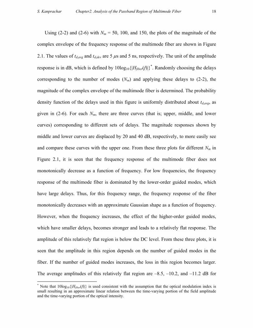
2.1 Magnitude response of the complex envelope of the multimode fiber modeled by (2-2): td,avg = 5 µs and td,dev = 5 ns. For each Nm, there are three curves (i.e.; upper, middle, and lower curves) corresponding to different sets of delays. The magnitude responses for middle and lower curves are displaced by 20 and 40 dB, respectively��������...... 17
2.2 Plots of normalized ( )fiberHR ν and ( ) ( ) 2
fiber fiberH f H f ν+ for Nm =
100 modes, td,avg = 5 µs and td,dev = 5 ns�������������� 30
2.3 Plots of normalized ( )fiberHR ν and ( ) ( ) 2
fiber fiberH f H f ν+ for Nm =
150 modes, td,avg = 5 µs and td,dev = 5 ns�������������� 31
3.1 Diagram of the transmission system using three subcarriers on multimode fiber.���������������������������.. 35
3.2 Magnitude responses of multimode fiber and subcarrier signals located at 0.5, 1.0, and 1.5 GHz..��������������������... 39
3.3 Eye-diagrams of received subcarrier signals: without electrical equalization and BWBP = 4Rb..�����������������... 40
3.4 Eye-diagrams of received subcarrier signals: with electrical equalization and BWEq = 4Rb����������������������..... 41
3.5 Eye-diagrams of the combined signal from three received subcarrier signals: without and with electrical equalization and BWBP = BWEq = 4Rb�������������.�������������........ 41
3.6 Illustration of the magnitude response of the ideal and limited-gain equalizers�������������.������������.. 45
3.7 Eye-diagrams of received subcarrier signals: with limited-gain electrical equalization (∆G = 0 dB) and BWEq = 4Rb������������� 46
ix
3.8 Eye-diagrams of combined signal from three received subcarrier signals: for different cases, BWBP = BWEq = 4Rb�������������� 46
4.1 Diagram of the transmission system using subcarrier frequency and direct sequence spread spectrum with the passband region of the multimode fiber�������������.��������������.. 54
4.2 Magnitude responses of the multimode fiber, the input signal, and the input spread spectrum (code length = 7) signal: First simulation����. 55
4.3 Eye-diagrams of the received signal in the first simulation: without and with spread spectrum (code length = 7) �������������... 55
4.4 Magnitude responses of the multimode fiber, the input signal, and the input spread spectrum (code length = 7) signal: Second simulation���. 56
4.5 Eye-diagrams of the received signal in the second simulation: without and with spread spectrum (code length = 7) �������������... 56
4.6 Histogram of the signal-to-noise ratio from 300 simulations: without and with spread spectrum (code length of 7 and 15) ����������.. 60
4.7 Histogram of the signal-to-noise ratio from 300 simulations: without and with spread spectrum (code length of 7 and 15) ����������.. 63
5.1 Diagram of the multimode fiber transmission using subcarrier multiplexing (SCM) �������������.�������� 68
5.2 Magnitude responses of 5 different sets ((a) to (e)) of frequency responses of multimode fiber; transmission bandwidth (Tx BW) is from 4.25 GHz to 7.5 GHz�������������.������������� 72
5.3 Bit-error-rate (BER) as a function of input optical power to the photodetector for fives fibers [(a) to (e)] for the number of subcarriers = 20�������������.��������������.�. 76
5.4 Bit-error-rate (BER) as a function of input optical power to the photodetector for fiber (a) to (e): for number of subcarriers = 10, 20, 30, 40, and 50�������������.������������.
79
x
6.1 Bit-error-rate (BER) as a function of input optical power to the photodetector for fiber(a) to fiber(e): without and with training sequence (2 channels dropped), and number of subcarriers = 10 and 40�����. 87
6.2 Bit-error-rate (BER) as a function of input optical power to the photodetector of 10-subcarrier SCM multimode fiber system for 5 different sets of multimode fiber: without and with training sequence (dropping 1, 2, and 3 channels) �������������.���... 89
7.1 Diagram of subcarrier multiplexed multimode fiber system with diversity coding�������������.�������������... 118
7.2 Comparison of performance of (1) no training sequence or diversity coding (No TS, No DC), (2) training sequence with two dropped channels, and (3) diversity coding with 2 parity channels. The five plots (a)-(e) correspond to the five different sets of multimode fiber from Figure 5.2�������������.������������. 120
7.3 Performance of the three system configurations indicating sensitivity to fiber frequency response�������������.������.. 121
8.1 Illustration of frequency response of multimode fiber due to modal and material dispersion�������������.��������... 132
8.2 Probability of having k subcarriers (from an N-subcarrier system) located at the nulls: for different values of N and �����������... 138
8.3 Probability of having k subcarriers (from an N-subcarrier system) located at the deep nulls (at least 10 dB below the average amplitude)����� 142
8.4 The number (k) of subcarriers located at deep nulls as a function of the total number (N) subcarriers: for different values of probabilities���� 143
8.5 Probability of having k subcarriers (from an N-subcarrier system) located at the deep nulls (at least 10 dB below the average amplitude) determined from Poisson distribution in (8-19).�������������.��. 148
8.6 The number (k) of subcarriers located at deep nulls as a function of the total number (N) subcarriers: from Binomial and Poisson distributions, p = 10-3�������������.�������������� 149

xi
8.7 The ratio between the number (k) of subcarriers located at deep nulls and the total number (N) of subcarriers as a function of the total number subcarriers: from Binomial and Poisson distributions, p = 10-3����� 150
8.8 Total received optical power, received optical DC power, and received optical AC power as a function of the fiber length���������... 159
8.9 The signal-to-noise ratio of the received subcarrier signal as a function of the fiber length�������������.����������. 160
8.10 The number of subcarriers as a function of the fiber length������. 161
8.11 The total bit rate as a function of the fiber length.���������� 163
A.1 Signal-to-noise ratio as a function of the bandwidth of bandpass filter: for different subcarriers�������������.��������.. 175
A.2 Signal-to-noise ratio as a function of the bandwidth of bandpass filter (or
the bandwidth of electrical equalizer): without and with electrical equalization�������������.�����������.. 176
B.1 Output signal-to-noise ratio as a function of ∆G: for limited-gain
equalization with BWEq = 4Rb�������������.����.. 180
B.2 Output signal-to-noise ratio (in dB) as a function of ∆G: for different subcarriers, BWEq = 4Rb�������������.������� 181

xii
LIST OF TABLES
7.1 All possible cosets related to 4( ) 1p x x x= + + �����������. 97
7.2 Exponential, polynomial, and vector-space representations of GF(24)�..... 102
7.3 List of symbols at transmitter, receiver, and output of the decoder for example 1: one failure data channel��������������...... 105
7.4 List of symbols at transmitter, receiver, and output of the decoder for example 2: two failure data channels��������������� 108
8.1 List of the maximum fiber length, the maximum bit rate, and the number
of subcarriers for different values of transmit optical power������ 169

S. Kanprachar Chapter 1. Introduction
1
Chapter 1
Introduction
The data rate required for local area networks has increased dramatically to over 1
Gbps. The only medium which can support such high data rate with small attenuation is
the optical fiber. However, optical fibers that are available in many buildings or LAN
links are multimode fibers, which normally have a baseband bandwidth-distance product
less than 500 MHz-km. If the data rate is 2.5 Gbps, the data can only be transmitted over
fiber lengths less than 200 m, which is too short for many applications. The bandwidth-
distance product has to be increased. Increasing this by replacing the multimode fiber
with a single mode fiber is generally too expensive. Moreover, the available multimode
fibers will then be wasted. Hence, how to achieve a high data rate (in Gbps) transmission
for a short distance (e.g., less than 10 km) on multimode fibers is a topic of considerable
interest. This dissertation focuses on the use of subcarrier multiplexing, utilizing carrier
frequencies above what is generally utilized for multimode fiber transmission, to achieve
high bit rates.
In this Chapter, a brief review of multimode fibers and previous research on
multimode fiber in high bit-rate transmission are given. This is followed by a discussion
of subcarrier multiplexing (SCM) and types of system modifications for improving the

S. Kanprachar Chapter 1. Introduction
2
performance of high bit-rate transmission on multimode fiber. Finally, the dissertation
objectives and organization of the dissertation are given.
1.1 Multimode Fiber in High Bit-Rate Transmission
Optical fibers can be categorized by the number of guided modes supported by the
fiber. There are two types of optical fibers; that is, single-mode fiber and multimode
fiber. For single-mode fibers, there is only one guided mode* supported by the fiber;
whereas for multimode fibers, more than one mode is supported by the fiber. The number
of guided modes in multimode fiber can be up to many hundreds of modes [1] and
depends on many factors, including operating frequency, the core diameter, type of
refractive index of the core (graded or step), and so on. The optical power from an optical
pulse launched into a multimode fiber is generally distributed over all of the guided
modes. These modes then propagate along the fiber to the receiving end, and in practical
systems there is often interchange of power between the modes (mode coupling). The
problem with multimode fiber is that the propagation velocity of each of the guided
modes is different. This means that at the receiving end, the received optical pulse is
spread out in time resulting in pulse dispersion. The pulse spread becomes larger if the
fiber length increases. This type of dispersion is called intermodal dispersion. This
dispersion is the main limitation of data transmission on multimode fiber. If the bit rate of
the transmit signal is high, the bit period is small. When a received pulse is spread out in
* Note that there are actually two modes corresponding to two orthogonal polarizations. If the group velocities for these two modes are different, a potential source of pulse broadening called the polarization-mode dispersion (PMD) can become a problem. Although PMD is of concern in high bit rate long distance systems, it is negligible for the systems considered in this dissertation.
S. Kanprachar Chapter 1. Introduction
3
time caused by intermodal dispersion, the neighboring pulses may overlap. This may lead
to a wrong decision in the decision circuit in the receiver; thus, a high bit-error-rate
(BER). This effect becomes more significant both as the bit rate and distance increase. In
practice, the intermodal bandwidth-distance product of a multimode fiber is specified.
The unit of this parameter is normally in MHz-km. The intermodal bandwidth
(BWintermodal) of a multimode fiber can be estimated from the full width at half maximum
of the received pulse (στ) [41] when the transmitted pulse is very narrow; that
is, intermodal 0.44BW τσ= .The typical value of the intermodal bandwidth-distance product
for a multimode fiber is between 300 to 500 MHz-km. For binary transmission the
maximum bit rate is of the order of the bandwidth, so that only about a 500-Mbps signal
can be sent over a transmission distance of 1 km. To achieve a higher bit rate, the
transmission distance has to be decreased. This is not a satisfactory situation since a high
bit rate signal can only be transmitted for a short distance.
To increase the bandwidth-distance product of multimode fibers, many approaches
have been suggested; for example, using an offset launch condition instead of over-filled
launch [2-9], using multi-level coding [7, 8], and using parallel optics with multimode
ribbon cable [8]. The offset launch is done by offsetting the launching spot from the core
center of the fiber. By doing this, the number of guided modes excited by the launch is
reduced and becomes smaller than the number of guided modes excited by the over-filled
launch. Hence, the pulse spreading from an offset launch is smaller and the bandwidth of
the fiber is increased. For multi-level coding, an m-ary modulation scheme with m>2 is
adopted. The bit rate of the signal to be sent over the fiber is increased since one

S. Kanprachar Chapter 1. Introduction
4
transmitted symbol contains more than 2 bits. For the technique using parallel optics with
multimode ribbon cable, a high bit rate signal is divided into many low bit rate signals
and these signals are transmitted simultaneously over the multimode ribbon cable.
However, in all of these three techniques, only the frequencies below the modal
bandwidth of the fiber are used. The frequencies higher than the modal bandwidth of the
fiber are not exploited. It has been shown in many papers [10-17] that the frequency
response of the multimode fiber does not monotonically decrease as the frequency
increases. The frequency response of the multimode fiber at low frequencies decreases
monotonically with frequency and can be modeled as a Gaussian shape. However, in the
high frequency range, the frequency response does not fall off but becomes relatively flat
with an amplitude of 6 to 10 dB below the amplitude at zero frequency. One interesting
approach to utilize this high frequency region is to use subcarrier multiplexing with the
multimode fiber. It has been shown that using subcarrier multiplexing within this high
frequency region, a high data rate can be successfully transmitted over a fiber length
larger than 400 meters. For example, in [7], a 1.25-Gbps signal is divided into two 625-
Mbps signals. One of these two signals is modulated onto a subcarrier frequency of 1
GHz and the other is modulated onto a subcarrier frequency of 3 GHz. These two
subcarrier signals are combined and sent to a laser to convert the subcarrier electrical
signal into an output optical signal. This optical signal is then transmitted over the high
frequency region of the multimode fiber. It has been shown that the total 1.25 Gbps
signal can be successfully transmitted over a fiber length of 500 m. The origin of the
passband region of the multimode fiber has been explained roughly as resulting from an
impulse response that is a series of delta functions with different delays corresponding to
S. Kanprachar Chapter 1. Introduction
5
different guided modes in the fiber when the mode coupling and chromatic dispersion are
ignored [11, 13]. The detailed explanation and analysis of this passband region is treated
in Chapter 2, and was reported in [18].
1.2 Subcarrier multiplexing (SCM) transmission on multimode fiber
Although the bandpass region of the multimode fiber is relatively flat with amplitude
of 6 to 10 dB below the amplitude at zero frequency, it may not be possible to use this
passband region to transmit a signal with bit rate large compared to 3-dB modal
bandwidth. The deep nulls and variation of the amplitude of the frequency response of
the multimode fiber within the transmission frequency can significantly degrade the
output signal of the multimode fiber; thus, leading to high BER at the receiver. It is seen
from [18] that the probability density function of the amplitude response of the
multimode fiber in the high frequency range is Rayleigh distributed and does not depend
on the frequency. This property of the bandpass region of the multimode fiber is similar
to the property of the channel in a wireless communications system; that is, the fiber is a
wideband frequency-selective channel. The effect of having a wideband frequency-
selective channel for data transmission can be overcome by using orthogonal frequency
division multiplexing (OFDM). This technique has been proposed and analyzed by many
groups of researchers [19-25]. In OFDM, the high data rate signal is divided into many
small data rate signals. These small data rate signals are then transmitted via different

S. Kanprachar Chapter 1. Introduction
6
subcarrier frequencies. By doing this the wideband frequency-selective channel is
separated into a series of many narrowband frequency-nonselective channels. The main
requirement of doing OFDM is the orthogonality between all OFDM signals in the
frequency domain. That is, the spectrum of each OFDM signal should not interfere with
the spectra of neighboring OFDM signals. To have completely non-overlapping spectra,
the required bandwidth of the system will then be large; that is, less spectral efficiency.
To increase the spectral efficiency of the system, the signal spectra must be packed
tightly. By doing this, very sharp filtering (which is very difficult to implement) is
needed; thus, more system complexity is required [19]. It is seen that using sharp filtering
is not a good way to increase the spectral efficiency of an OFDM system. Other
approaches are given in [19] to [25]. In [19], it is shown that using Staggered Quadrature
Amplitude Modulation (SQAM) can increase the spectral efficiency of the OFDM
system. The subcarriers are located exactly at the nulls of the immediate neighboring
spectra. Each spectrum overlaps only its immediate neighbors. Orthogonality of spectra is
achieved by staggering the data on alternate in-phase and quadrature channels. However,
the amount of the filtering used in this technique is still considerable so it is not widely
used. Another technique is to make the individual spectra to be sinc functions. The
subcarriers are put at the nulls of the neighboring spectra. It is seen that the OFDM
spectra are not bandlimited but they can be separated by the baseband processing using
discrete-Fourier transform (DFT) techniques [19-23]. The detailed analysis of using DFT
for OFDM system is given in [22] and [23]. The applications of using OFDM with fiber-
optic transmission have been shown in [24] and [25]. OFDM was used in the subcarrier
multiplexed fiber-optic video transmission as a digital transmission scheme of the hybrid

S. Kanprachar Chapter 1. Introduction
7
AM/OFDM system [24]. The performance of the OFDM system was given and compared
to the performance of a conventional QAM system. It has been shown that the OFDM
technique provides much better performance. This is because the period of an OFDM
symbol is much longer than the period of a QAM symbol. The clipping impulse noise
only affects a small fraction of an OFDM symbol. Another example of using OFDM with
a fiber-optic system is shown in [25]. The multimode fiber is used as an inexpensive cell
feed in broad-band 60-GHz indoor picocellular systems. To overcome the effect of
multipath fading in a wireless environment, OFDM is chosen to be the modulation
scheme for the wireless transmission. However, to reduce the complexity required by the
remote site, the signal modulation should be done at the central office and sent from the
central office to the remote site via an optical fiber system. Using multimode fiber as the
medium instead of singlemode fiber can reduce the cost of implementing the optical fiber
system. However, the problem of using multimode fiber as the medium is the effect of
the dispersion in multimode fiber. Since the multipath problems in wireless system can be
overcome by the use of OFDM, OFDM might also be able to reduce the effect of
frequency selectivity in the dispersive multimode fiber. It was shown in [25] that OFDM
can offer good protection against the frequency selectivity of the dispersive multimode
fiber. Thus, the seamless transition between the fiber and radio parts of the system with
an inexpensive cost for the fiber part is possible.
It is seen that the key point for combating a wideband frequency-selective channel,
such as occurs for high frequencies in multimode fiber, is to divide a high bit rate signal

S. Kanprachar Chapter 1. Introduction
8
into many small bit rate signals and transmit these signals with different subcarriers. By
doing this, the wideband frequency-selective channel is transformed into a series of
narrowband non-selective channels. Applying this idea to the multimode fiber
transmission in the high frequency region, OFDM is a good approach. However, since the
available bandpass bandwidth of multimode fiber is very large, the orthogonality between
subcarriers is easily achieved by increasing the frequency separation between two
consecutive subcarriers. There is no need to tightly put subcarriers in a specific
bandwidth. The sharp filtering is then not required. Consequently, it is seen that it may be
possible to use subcarrier multiplexing (SCM) to transmit a high bit rate signal over the
high frequency region of multimode fiber, but there are many open questions concerning
the design of such systems, e.g., the frequency response at frequencies above the
intermodal bandwidth limit, the total available bandwidth, the bit rate that may be
transmitted on each subcarrier, the number of subcarriers that may be used, the coding
across multiple subcarriers to improve performance, and the total bit rates and distances
that may be achieved. This dissertation will be devoted mainly to answering these
questions.
1.3 System modifications for improving the system performance
Even though using OFDM and/or SCM, the wideband frequency-selective channel
can be transformed into a series of narrowband frequency-nonselective channels, this
does not guarantee that the subcarriers will not be placed at the nulls of the frequency

S. Kanprachar Chapter 1. Introduction
9
response. If this happens, the signal performance at the receiver end will be degraded
significantly. There are many techniques to improve the signal performance. A good
approach is using channel encoding. With this approach, errors in the received signal can
be corrected at the receiver. Many types of channel encodings have been applied to
OFDM systems; for example, block code [26], convolutional code [27, 28], Trellis-code
modulation [29], Reed-Solomon code with Trellis-code modulation [30]. The received
signal is surely improved since there is some redundancy systematically added to the
signal. However, with these coding techniques, the effect of having subcarriers located
near the deep nulls of the frequency response of the multimode fiber may not be totally
canceled.
Another approach might be using electrical equalization at the receiving end. With
this approach, the property of each subcarrier channel has to be determined so that an
electrical equalizer for each such channel can be constructed. The equalizer will undo
what the channel has done to the signal. The attenuated pulse can be retrieved completely
even if the subcarrier is at a deep null. However, noise can become a main problem since
the gain of the equalizer will be very high, if the subcarrier is located at a deep null. The
effects of adding electrical equalization at the receiver are studied in Chapter 3.
Spreading the spectrum of the transmitted signal by using direct sequence spread
spectrum might be a good technique to improve the system performance since there will
be more passband regions covered by the signal spectrum; that is, obtaining the effect of
frequency diversity. The amplitude of each frequency component is small and if there is a

S. Kanprachar Chapter 1. Introduction
10
frequency component located at a null, the degradation from such null to the overall
received signal should be small. The effects of using direct sequence spread spectrum
with multimode fiber system are studied in Chapter 4.
It is shown in Chapters 3 and 4 that adding electrical equalization to the receiver
and/or using the direct sequence spread spectrum do not really eliminate the effect of
having some subcarriers located at deep nulls. A better way to completely remove the
effects of these nulls might be the use of a training sequence to determine the properties
of subcarrier channels. With the training sequence, the subcarrier channels to be used for
signal transmission will be determined during the training process. With this technique,
any bad channels (which are normally located near the deep nulls) will not be used for
transmission; thus, the effect of the nulls is completely removed. However, using training
sequence requires more system complexity. It requires more channels during the training
process since some of channels will be dropped out after the training process. And, if the
channels are time-varying, the training process must be done frequently to update the
channels’ properties. This is not good for real-time communications. Also, the transmitter
must be able to re-locate the subcarriers for data transmission if the channels are time-
varying.
To reduce the system complexity and eliminate the effect of the nulls in the frequency
response of the multimode fiber, another technique has to be used. It is shown in [31] that
diversity coding is very useful for self-healing communication networks. This technique
is accomplished by adding parity symbols and parity channels; that is, more channels are

S. Kanprachar Chapter 1. Introduction
11
needed. The parity symbols are generated from the data symbols from all data channels.
By doing this, at the receiver, the data received from the poorest channels (decided by the
signal-to-noise ratios of all received subcarrier signals) will be totally disregarded. The
lost data from these poorest channels will be recovered by the data received from other
good channels at the decoder. Applying this technique to the SCM multimode fiber
system, it is seen that if there are some channels located near the nulls of the multimode
fiber, the data received from those channels will not be taken into account as a part of the
received signal. Thus, the effect of the deep nulls in the multimode fiber is totally
removed. Using this diversity coding, there is no need to update the channels’ properties
and there is no need to have the ability to re-locate the subcarriers for data transmission
since any lost data can be recovered instantaneously at the receiver; that is, less system
complexity compared to that required by using training sequence with SCM multimode
fiber system.
1.4 Objectives and Organization of Dissertation
From the previous discussion, it is seen that the frequency response of multimode
fiber, which seems to decrease as the frequency increases, becomes relatively flat as the
frequency increases beyond the intermodal bandwidth. It is important then to study
analytically the frequency response of multimode fiber at high frequencies and determine
how a high bit rate signal can be transmitted efficiently using this frequency region.
Another important topic is the limitations on the performance that may be achieved with

S. Kanprachar Chapter 1. Introduction
12
bandpass transmission on multimode fiber. Based on this discussion, the following major
research objectives are established.
(1) Study of the statistical properties of frequency response of multimode fiber at
high frequencies,
(2) Study of different transmission approaches for transmitting a signal using the
bandpass region of multimode fiber,
(3) Study of the system modifications for improving the performance of subcarrier
multiplexed system on multimode fiber, and
(4) Study of the practical performance limits and system capacity of subcarrier
multiplexed system on multimode fiber.
The organization of the dissertation is as follows. In Chapter 1, a brief review of
multimode fiber and the recent research on how to transmit the high bit rate signal are
given. Also, the discussion about possible types of transmission and system modifications
are given. In Chapter 2, the frequency response of multimode fiber at high frequencies is
analyzed and modeled. The statistical properties of multimode fiber in the high frequency
region are given. Chapter 3 presents the simulation results of having electrical
equalization added to the receiver for a three-subcarrier system. The simulation results
for the multimode fiber using spread spectrum are given in Chapter 4. It is found that
using electrical equalization or using spread spectrum with bandpass transmission on

S. Kanprachar Chapter 1. Introduction
13
multimode fiber does not give good system performance. The main focus of the
dissertation is in Chapters 5 to 8. In Chapter 5, the subcarrier multiplexing (SCM) is
applied to the multimode fiber system. The simulation results of bit-error-rate (BER) for
different numbers of subcarriers are shown. The improvements of using training sequence
and diversity coding with SCM multimode fiber system are presented in Chapters 6 and
7, respectively. The practical performance limits and system capacity of SCM multimode
fiber system is discussed in Chapter 8. And, finally, the summary and conclusions of the
dissertation are given in Chapter 9.

S. Kanprachar Chapter2. Analysis of the Passband Region of Multimode Fiber
14
Chapter 2
Analysis of the Passband Region of Multimode Fiber
2.1 Introduction
It has been shown in many papers [10-17] that the frequency response of the
multimode fiber does not monotonically decrease as the frequency increases. At high
frequency region, the frequency response of multimode fiber is relatively flat with an
amplitude 6 to 10 dB below the amplitude at zero frequency. There are many passbands
available at high frequencies. These passbands can be used as transmission channels for
sending the data. To make use of these passbands effectively, it is useful to understand
the characteristics of these passbands. The origin of these passbands has been explained
roughly as resulting from a series of delta functions with different delays corresponding
to different guided modes in the fiber when the mode coupling and chromatic dispersion
are ignored [11, 13]. However, this does not give any insight into the detail about these
passbands. To understand clearly about such passbands, a detailed analysis of the
frequency response of multimode fiber at high frequencies has to be done. In the
following sections in this chapter, the frequency response of multimode fiber at high
frequencies is modeled and analyzed [18]. Statistical properties of the bandpass regions
are also determined.

S. Kanprachar Chapter2. Analysis of the Passband Region of Multimode Fiber
15
2.2 Model of the Multimode Fiber
Using the suggestion in [11] and [13], the impulse response of the complex
envelope of the multimode fiber with Nm guided modes is just the combination of the
delta functions corresponding to different delays; that is,
( ) ( ),1
mN
fiber d nn
h t t tδ=
= −∑ (2-1)
Taking the Fourier transform of the impulse response in (2-1), the frequency response of
the complex envelope of the multimode fiber with Nm guided modes is given by
,2
1( )
md n
Nj f t
fibern
H f e π− ⋅
=
= ∑ (2-2)
To find the delay for a particular guided mode, the normalized propagation constant
(b) or the propagation constant (β) or the modal index ( )n for that mode have to be
determined by solving the eigenvalue equation for that mode. The time delay is given by
( )/d
Ltc n
= (2-3)
and 0 2 2
1 2 1 2
/ k n n nbn n n n
β − −= =
− − (2-4)
where L is the fiber length
c is the speed of light in free-space
k0 is the free-space wave number defined as 02k πλ
= (2-5)

S. Kanprachar Chapter2. Analysis of the Passband Region of Multimode Fiber
16
From (2-2), it is seen that to get the frequency response of the multimode fiber, the
delays for all Nm guided modes have to be found; that is, the modal index of each guided
mode has to be found. However, for practical multimode fibers the number of guided
modes has to be large to avoid modal noise; thus, many time delays have to be
determined in order to construct the frequency response. In the following analysis, the
time delays are modeled to be independent realizations of a random variable, which is
uniformly distributed about td,avg with the maximum deviation of td,dev; the probability
density function of td,n is given by
( ),
, , , , ,,,
1 ; for 2
0 ; elsewhere d n
d avg d dev d n d avg d devd devt d n
t t t t ttf t
− ≤ ≤ +=
(2-6)
Note that td,avg and td,dev depend on the fiber length, the number of guided modes, and the
refractive index profile of the fiber.

S. Kanprachar Chapter2. Analysis of the Passband Region of Multimode Fiber
17
0 0.5 1 1.5 2 2.5 3−60
−50
−40
−30
−20
−10
0N
m = 50 modes
frequency (GHz)
|Hfi
ber(f
)| (i
n dB
)
0 0.5 1 1.5 2 2.5 3−60
−50
−40
−30
−20
−10
0N
m = 100 modes
frequency (GHz)
|Hfi
ber(f
)| (i
n dB
)
0 0.5 1 1.5 2 2.5 3−60
−50
−40
−30
−20
−10
0N
m = 150 modes
frequency (GHz)
|Hfi
ber(f
)| (i
n dB
)
Figure 2.1 Magnitude response of the complex envelope of the multimode fiber modeled by (2-2): td,avg = 5 µs and td,dev = 5 ns. For each Nm, there are three curves (i.e.; upper, middle, and lower curves) corresponding to different sets of delays. The magnitude responses for middle and lower curves are displaced by 20 and 40 dB, respectively.
S. Kanprachar Chapter2. Analysis of the Passband Region of Multimode Fiber
18
Using (2-2) and (2-6) with Nm = 50, 100, and 150, the plots of the magnitude of the
complex envelope of the frequency response of the multimode fiber are shown in Figure
2.1. The values of td,avg and td,dev are 5 µs and 5 ns, respectively. The unit of the amplitude
response is in dB, which is defined by 10log10{|Hfiber(f)|}*. Randomly choosing the delays
corresponding to the number of modes (Nm) and applying these delays to (2-2), the
magnitude of the complex envelope of the multimode fiber is determined. The probability
density function of the delays used in this figure is uniformly distributed about td,avg, as
given in (2-6). For each Nm, there are three curves (that is; upper, middle, and lower
curves) corresponding to different sets of delays. The magnitude responses shown by
middle and lower curves are displaced by 20 and 40 dB, respectively, to more easily see
and compare these curves with the upper one. From these three plots for different Nm in
Figure 2.1, it is seen that the frequency response of the multimode fiber does not
monotonically decrease as a function of frequency. For low frequencies, the frequency
response of the multimode fiber is dominated by the lower-order guided modes, which
have large delays. Thus, for this frequency range, the frequency response of the fiber
monotonically decreases with an approximate Gaussian shape as a function of frequency.
However, when the frequency increases, the effect of the higher-order guided modes,
which have smaller delays, becomes stronger and leads to a relatively flat response. The
amplitude of this relatively flat region is below the DC level. From these three plots, it is
seen that the amplitude in this region depends on the number of guided modes in the
fiber. If the number of guided modes increases, the loss in this region becomes larger.
The average amplitudes of this relatively flat region are –8.5, –10.2, and –11.2 dB for * Note that 10log10{|Hfiber(f)|} is used consistent with the assumption that the optical modulation index is small resulting in an approximate linear relation between the time-varying portion of the field amplitude and the time-varying portion of the optical intensity.

S. Kanprachar Chapter2. Analysis of the Passband Region of Multimode Fiber
19
Nm = 50, 100, and 150, respectively. Considering the passband bandwidth in each case, it
is seen that there are many bandpass regions that have in total a much larger bandwidth
than the 3-dB baseband bandwidth. For example, for Nm = 50 (upper curve), the bandpass
regions, which have large passband, are at 0.24, 0.5, 0.8, 1.25, 1.5, 1.7, 2.3, and 2.8 GHz.
The bandwidth from these passbands is approximately 1.5 GHz (estimated from the
regions where the response is greater than –10 dB). It is seen that just from these eight
passbands, the available bandwidth is much larger than the baseband bandwidth, which is
approximately 100 MHz. Thus, the data rate can be increased significantly if these
passband regions of the multimode fiber are used. It should be noted that comparing the
magnitude responses from different sets of delays for each Nm, it is seen that the shapes of
the responses at low frequencies (baseband region) are almost identical. At high
frequencies, although the locations of the passband regions are not identical for these
three sets of delays, the structure of these passband regions are the same; that is, they are
relatively flat with the same average value.
2.3 Analysis of statistical properties of the multimode fiber at high frequency
2.3.1 Probability density function of the magnitude response of the multimode fiber
From (2-2), we get
( ) ( ) ( )2 2 2 2
, ,1 1 1 1cos 2 sin 2
m m m mN N N N
fiber d n d n n nn n n n
H f ft ft x yπ π= = = =
= + = +
∑ ∑ ∑ ∑ (2-7)
where ( ) ( ), ,cos 2 and sin 2n d n n d nx ft y ftπ π= =

S. Kanprachar Chapter2. Analysis of the Passband Region of Multimode Fiber
20
Letting ,2 d nftϕ π= , it follows that
( )( ) ( ), , , ,
,
1 ; for 2 24
0 ; elsewhere
d avg d dev d avg d devd dev
f t t f t tftfϕ
π ϕ ππϕ
− ≤ ≤ +=
(2-8)
Thus, we get ( ) ( )cos nx gϕ ϕ= = ; ,min ,max1 1n n nx x x− ≤ ≤ ≤ ≤ (2-9)
where xn,min and xn,max depend on 2πftd,avg and 2πf(2td,dev). If 2πf(2td,dev) ≥ 2π, 1 1nx− ≤ ≤ .
Considering n = 1, we get
( ) ( ) 21' sin 1g xϕ ϕ= − = − − (2-10)
and, ( )11cos ; 1,2,3,...,m sx m Mϕ −= = (2-11)
where Ms is the total number of ϕm satisfying (2-11).
Note that Ms depends on the value of x1 and 2πf(2td,dev); that is,
0 < 2πf(2td,dev) ≤ π or 0 < f ≤ ,
14 d devt
⇒ Ms = 1 or 2 (depending on f and x1)
π < 2πf(2td,dev) ≤ 2π or ,
14 d devt
< f ≤ ,
12 d devt
⇒ Ms = 2 or 3 (depending on f and x1)
2π < 2πf(2td,dev) ≤ 3π or,
12 d devt
< f ≤ ,
1
d devt ⇒ Ms = 3 or 4 (depending on f and x1)
and so on.
Given td,avg and td,dev, it is seen that Ms depends on x1 and f. The probability density
function of x1 is given by
( ) ( )( )1 1
1 '
sMm
xm m
ff x
gϕ ϕ
ϕ=
= ∑ (2-12)

S. Kanprachar Chapter2. Analysis of the Passband Region of Multimode Fiber
21
Using (2-8) and (2-10) with (2-12), we get
( )1 1 2
,1
141
sx
d dev
Mf xftx π
= ⋅−
(2-13)
Considering the case where the frequency is very large (passband region); i.e.,
,
12 d dev
ft
>> ; we get that
, ,2 2 4s d dev d devM f t ft ≅ ⋅ = (2-14)
Substituting (2-14) into (2-13), the probability density function of x1 at high frequency is
given by
( )1 1 12
1
1 ; 1 11
xf x xxπ
= − ≤ ≤−
(2-15)
The mean and variance of x1, obtained from the probability density function given in
(2-15) are 0 and 0.5, respectively.
Note that the probability density function of each xn is also given by (2-15).
Let 1
mN
nn
X x=
= ∑ (2-16)
With large Nm, the probability density function of X can be determined by using the
central limit theorem; that is, we get
( )( )2
2212
X
X
X m
XX
f X e σ
σ π
− −
≅ (2-17)
where 1 1
0 0m m
n
N N
X xn n
m m= =
= = =∑ ∑ . (2-18)
and, 2 2
1 10.5
2
m m
n
N Nm
X xn n
Nσ σ= =
= = =∑ ∑ (2-19)

S. Kanprachar Chapter2. Analysis of the Passband Region of Multimode Fiber
22
Similarly, for the sine terms in (2-7) or yn, we get that for a high frequency, the
probability density function of yn is approximated by
( )2
1 ; 1 11ny n n
n
f y yyπ
= − ≤ ≤−
(2-20)
The mean and variance of yn given in (2-20) are 0 and 0.5, respectively.
Let 1
mN
nn
Y y=
= ∑ (2-21)
With large Nm, the probability density function of Y can similarly be determined by using
the central limit theorem; that is, we get
( )( )2
2212
Y
Y
Y m
YY
f Y e σ
σ π
− −
≅ (2-22)
where 1 1
0 0m m
n
N N
Y yn n
m m= =
= = =∑ ∑ . (2-23)
and, 2 2
1 10.5
2
m m
n
N Nm
Y yn n
Nσ σ= =
= = =∑ ∑ (2-24)
From (2-17) to (2-24), the probability density functions of X and Y are normal
distributions with zero mean and variance of Nm/2. Also, X and Y are independent since X
is from the cosine terms of td,n and Y is from the sine terms of td,n. Thus, using these
properties with (2-7), the probability density function of ( )fiberH f at the high frequency
range is given by
( ) ( )( ) ( ) ( )( )( )
2
2 2exp2fiber
fiber fiberfiber fiberH f
X X
H f H ff H f U H f
σ σ
− =
( ) ( )( )( )
22
expfiber fiberfiber
m m
H f H fU H f
N N
− =
(2-25)

S. Kanprachar Chapter2. Analysis of the Passband Region of Multimode Fiber
23
where U is the unit step function.
Note that the density function given in (2-25) is the Rayleigh density function.
From (2-25), the mean and the variance of ( )fiberH f are given by
( ) 2 2 2 4fiber
m mXH f
N Nm π π πσ= = = (2-26)
( )
2 22 2 12 2 2 4H ffiber
mX m
N Nπ π πσ σ = − = − = − (2-27)
Using (2-26), the mean value of ( )fiberH f compared to the maximum value of
( )fiberH f at f = 0 is given by
( ) ( ) ( )10 10 10
1in dB 10log 10log 10log4 4
fiber
fiber
H f mH f
m m m
m NmN N N
π π = = =
(2-28)
which indicates that the mean value decreases as Nm increases, consistent with Figure 2.1.
For example, (2-28) indicates that for Nm = 100, the mean value of ( )fiberH f is –10.5
dB and for Nm = 150, the mean value of ( )fiberH f is –11.4 dB.
2.3.2 Correlation function of the frequency response
Another important statistical parameter is the correlation function since this
influences the bandwidth at high frequency. In this section, the correlation function of the
frequency response of the multimode fiber ( ( )fiberHR ν ) is determined.

S. Kanprachar Chapter2. Analysis of the Passband Region of Multimode Fiber
24
From (2-7), we get
( ) ( ) ( ) ( ) ( ), ,1 1cos 2 sin 2
m mN N
fiber d n d nn n
H f ft j ft X f jY fπ π= =
= + = +∑ ∑ (2-29)
And, ( ) ( ) ( )νν += fHfHR fiberfiberH fiber
* { }{ })()()()( νν +−++= fjYfXfjYfX
[ ])()()()()()()()( νννν +−+++++= fYfXfXfYjfYfYfXfX (2-30)
From (2-30), we get that 0)()()()( =+=+ νν fYfXfXfY since the averages of X
and Y are zero and they are uncorrelated to one another. And,
( ) ( ), ,1 1
( ) ( ) cos 2 cos 2 ( )m mN N
d n d mn m
X f X f ft f tν π π ν= =
+ = +
∑ ∑
( )( ) ( )( ), , , , , ,1 1
1 cos 2 cos 22
m mN N
d n d m d m d n d m d mn m
f t t t f t t tπ ν π ν= =
= + + + − − ∑∑
Since we are interested in the properties of the multimode fiber at high frequency, it is
reasonable to assume that devdt
f,2
1>> (see the discussion in (2-10) to (2-14)). However,
if ν is very large (i.e., ν is also much greater thandevdt ,2
1 ), the frequency response at
frequency f + ν will be independent of the frequency response at frequency f.
Consequently, we are concerned with devdt ,2
1<ν . Using these two inequalities, we get
that
( )( ), , ,1 1
1( ) ( ) cos 22
m mN N
d n d m d mn m
X f X f f t t tν π ν= =
+ = − − ∑∑ (2-31)
Considering (2-31), it is seen that if m ≠ n, [ ]( )( ) 02cos ,,, =−− mdmdnd tttf νπ ; thus,

S. Kanprachar Chapter2. Analysis of the Passband Region of Multimode Fiber
25
( ) ( ) ( ) ( ), ,1 1
1 1cos 2 cos 22 2
m mN N
d n d nn n
X f X f t tν πν πν= =
+ = =∑ ∑ (2-32)
Similarly, for the term )()( ν+fYfY , we get that
( ) ( ), ,1 1
( ) ( ) sin 2 sin 2 ( )m mN N
d n d mn m
Y f Y f ft f tν π π ν= =
+ = +
∑ ∑
( )( ) ( )( ), , , , , ,1 1
1 cos 2 cos 22
m mN N
d n d m d m d n d m d mn m
f t t t f t t tπ ν π ν= =
= − − − + + ∑∑
Assumingdevdt
f,2
1>> , and
devdt ,21
<ν , we get that
( )( ) ( ), , , ,1 1 1
1 1( ) ( ) cos 2 cos 22 2
m m mN N N
d n d m d m d nn m n
Y f Y f f t t t tν π ν πν= = =
+ = − − = ∑∑ ∑ (2-33)
Therefore,
( ) ( ) ( ) ( )*,
1cos 2
m
fiber
N
H fiber fiber d nn
R H f H f tν ν πν=
= + = ∑ (2-34)
2.3.3 Correlation function of the magnitude response
Although the correlation function of the frequency response is of interest, the
correlation function of the magnitude of the frequency response is of greater interest.
Using a similar approach to that in the previous section, we get that
( ) ( ) ( ) ( ) ( ) ( )2 * *fiber fiber fiber fiber fiber fiberH f H f H f H f H f H fν ν ν+ = + +
[ ][ ][ ][ ]1 1 1 1 2 2 2 2 X jY X jY X jY X jY= + − + −
( ) ( ) 2 2 2 2 2 2 2 2 21 2 1 2 1 2 2 1fiber fiberH f H f X X Y Y X Y X Yν+ = + + + (2-35)

S. Kanprachar Chapter2. Analysis of the Passband Region of Multimode Fiber
26
where ( ) ( )1 , 1 ,1 1cos 2 ; sin 2
m mN N
d n d nn n
X ft Y ftπ π= =
= =∑ ∑ (2-36)
and ( )( ) ( )( )2 , 2 ,1 1cos 2 ; sin 2
m mN N
d n d nn n
X f t Y f tπ ν π ν= =
= + = +∑ ∑ (2-37)
Considering each term in (2-35), we get that
-For 2 21 2X X ;
( ) ( )( )2 2
2 21 2 , ,
1 1cos 2 cos 2
m mN N
d n d mn m
X X ft f tπ π ν= =
= +
∑ ∑
( ) ( )( )2
, ,1 1
cos 2 cos 2m mN N
d n d mn m
ft f tπ π ν= =
= +
∑∑
( ) ( )( ) ( ) ( )( ), , , ,1 1 1 1
cos 2 cos 2 cos 2 cos 2m m m mN N N N
d n d m d q d rn m q r
ft f t ft f tπ π ν π π ν= = = =
= + +
∑∑ ∑∑
( )( ) ( )( )
( )( ) ( )( )
2 21 2 , , , , , ,
1 1
, , , , , ,1 1
1 cos 2 cos 24
cos 2 cos 2
m m
m m
N N
d n d m d m d n d m d mn m
N N
d q d r d r d q d r d rq r
X X f t t t f t t t
f t t t f t t t
π ν π ν
π ν π ν
= =
= =
= + + + − −
× + + + − −
∑∑
∑∑(2-38)
There are four terms in (2-38); that is,
( )( ) ( )( )( ) ( )( )
( ) ( )( )
, , , , , ,, , , 1
, , , , , ,
, , , 1, , , , , ,
cos 2 cos 2
cos 21 2 cos 2
m
m
N
d n d m d m d q d r d rm n q r
N d n d m d q d r d m d r
m n q rd n d m d q d r d m d r
f t t t f t t t
f t t t t t t
f t t t t t t
π ν π ν
π ν
π ν
=
=
⇒ + + + +
+ + + + + =
+ + − − + −
∑
∑
Assuming devdt
f,2
1>> , and
devdt ,21
<ν ; we get that

S. Kanprachar Chapter2. Analysis of the Passband Region of Multimode Fiber
27
( )( ) ( )( )
( ) ( )( )
, , , , , ,, , , 1
, , , , , ,, , , 1
cos 2 cos 2
1 cos 22
m
m
N
d n d m d m d q d r d rm n q r
N
d n d m d q d r d m d rm n q r
f t t t f t t t
f t t t t t t
π ν π ν
π ν
=
=
+ + + +
= + − − + −
∑
∑
( )( )2, ,
1 1
1 cos 22
m mN N
m d m d rm r
N t tπν= =
= + −
∑∑ (2-39)
( )( ) ( )( )( ) ( )( )
( ) ( )( )
, , , , , ,, , , 1
, , , , , ,
, , , 1, , , , , ,
cos 2 cos 2
cos 21 2 cos 2
m
m
N
d n d m d m d q d r d rm n q r
N d n d m d q d r d m d r
m n q rd n d m d q d r d m d r
f t t t f t t t
f t t t t t t
f t t t t t t
π ν π ν
π ν
π ν
=
=
⇒ + + − −
+ + − + − =
+ + − + + +
∑
∑
Assumingdevdt
f,2
1>> , and
devdt ,21
<ν ; we get that
( )( ) ( )( ), , , , , ,, , , 1
cos 2 cos 2 0mN
d n d m d m d q d r d rm n q r
f t t t f t t tπ ν π ν=
+ + − − = ∑ (2-40)
( )( ) ( )( )( ) ( )( )
( ) ( )( )
, , , , , ,, , , 1
, , , , , ,
, , , 1, , , , , ,
cos 2 cos 2
cos 21 2 cos 2
m
m
N
d n d m d m d q d r d rm n q r
N d n d m d q d r d m d r
m n q rd n d m d q d r d m d r
f t t t f t t t
f t t t t t t
f t t t t t t
π ν π ν
π ν
π ν
=
=
⇒ − − + +
− + + − − =
+ − − − − +
∑
∑
Assumingdevdt
f,2
1>> , and
devdt ,21
<ν ; we get that
( )( ) ( )( ), , , , , ,, , , 1
cos 2 cos 2 0mN
d n d m d m d q d r d rm n q r
f t t t f t t tπ ν π ν=
− − + + = ∑ (2-41)

S. Kanprachar Chapter2. Analysis of the Passband Region of Multimode Fiber
28
( )( ) ( )( )( ) ( )( )
( ) ( )( )
, , , , , ,, , , 1
, , , , , ,
, , , 1, , , , , ,
cos 2 cos 2
cos 21 2 cos 2
m
m
N
d n d m d m d q d r d rm n q r
N d n d m d q d r d m d r
m n q rd n d m d q d r d m d r
f t t t f t t t
f t t t t t t
f t t t t t t
π ν π ν
π ν
π ν
=
=
⇒ − − − −
− + − − + =
+ − − + − −
∑
∑
Assumingdevdt
f,2
1>> , and
devdt ,21
<ν ; we get that
( )( ) ( )( )
( )( ) ( )( )
, , , , , ,, , , 1
2, , , ,
1 1 1 1
cos 2 cos 2
1 2 cos 2 cos 22
m
m m m m
N
d n d m d m d q d r d rm n q r
N N N N
d m d r m d m d rm r m r
f t t t f t t t
t t N t t
π ν π ν
πν πν
=
= = = =
− − − −
= + + + −
∑
∑∑ ∑∑
(2-42)
Substituting (2-39) to (2-42) into (2-38), we get
( )( ) ( )( )22 21 2 , , , ,
1 1 1 1
1 cos 2 cos 24
m m m mN N N N
d m d r m d m d rm r m r
X X t t N t tπν πν= = = =
= + + + −
∑∑ ∑∑
(2-43)
-For 2 21 2Y Y ; using the same approach as we did for 2 2
1 2X X , we get
( )( ) ( )( )22 21 2 , , , ,
1 1 1 1
1 cos 2 cos 24
m m m mN N N N
d m d r m d m d rm r m r
Y Y t t N t tπν πν= = = =
= + + + −
∑∑ ∑∑
(2-44)
-For 2 21 2X Y and 2 2
2 1X Y ; since X and Y are independent to one another, we get
2 2 2 2 2 2 2 21 2 1 2 2 1 2 1 and X Y X Y X Y X Y= = (2-45)

S. Kanprachar Chapter2. Analysis of the Passband Region of Multimode Fiber
29
Using the results from (2-19) and (2-24); that is, 2 2
2mNX Y= = ; we get that
2
2 2 2 21 2 2 1 2 2 4
m m mN N NX Y X Y= = ⋅ = (2-46)
Substituting (2-43), (2-44), and (2-46) into (2-35), we get
( ) ( ) ( )( ) ( )( )2 2, , , ,
1 1
1 cos 2 cos 22
m mN N
fiber fiber m d m d r d m d rm r
H f H f N t t t tν πν πν= =
+ = + + + −∑∑
(2-47)
Using the results from (2-34) and (2-47) with td,avg = 5 µs, td,dev = 5 ns, the plots of
( )fiberHR ν and ( ) ( ) 2
fiber fiberH f H f ν+ as a function of frequency ν for the number of
guided modes (Nm), and normalized by Nm and 2Nm2, respectively, are shown in Figure
2.2 and 2.3. From the plots, the shapes of ( )fiberHR ν and ( ) ( ) 2
fiber fiberH f H f ν+ for
different number of guided modes (Nm) are almost identical. As the frequency (ν)
increases, the values of normalized ( )fiberHR ν and ( ) ( ) 2
fiber fiberH f H f ν+ approach 0
and 0.5, respectively. Considering the plot of ( ) ( ) 2
fiber fiberH f H f ν+ , the available
bandwidth is approximately 100 MHz (two times the width of the autocorrelation
function), which is comparable to the 3-dB modal bandwidth found from Figure 2.1. Note
that from (2-34) and (2-47) it is seen that to get larger bandwidth, the maximum delay
deviation (td,dev) should be reduced. The value of the maximum delay deviation used in
this chapter is for illustrative purposes only; actual values will depend on the fiber type
and length.

S. Kanprachar Chapter2. Analysis of the Passband Region of Multimode Fiber
30
From the results found in (2-25), (2-28), (2-34), and (2-47), it is seen that to get a
high average value of ( )fiberH f at high frequency and large available passband
bandwidth, the number of guided modes and the maximum delay deviation should be
decreased. However, if the number of guided modes is too small, another impairment
namely modal noise becomes stronger and can degrade the system performance. In
practice, the effective number of modes will be less than the actual number of modes
since all modes are not equally excited, and modes near cut-off will have higher
attenuation. In the model considered here, all modes are assumed to have equal
amplitude. The effective number of modes in multimode fiber used for communications
is of the order of 100.
0 50 100 150 200 250 300 350 400
−0.2
0
0.2
0.4
0.6
0.8
ν (MHz)
RH
fibe
r(ν)
0 50 100 150 200 250 300 350 4000.4
0.5
0.6
0.7
0.8
0.9
1
ν (MHz)
<|H
(f)H
(f+ν
)|2 >
Figure 2.2 Plots of normalized ( )
fiberHR ν and ( ) ( ) 2
fiber fiberH f H f ν+ for Nm =
100 modes, td,avg = 5 µs and td,dev = 5 ns.

S. Kanprachar Chapter2. Analysis of the Passband Region of Multimode Fiber
31
0 50 100 150 200 250 300 350 400
−0.2
0
0.2
0.4
0.6
0.8
1
ν (MHz)
RH
fibe
r(ν)
0 50 100 150 200 250 300 350 4000.4
0.5
0.6
0.7
0.8
0.9
1
ν (MHz)
<|H
(f)H
(f+ν
)|2 >
Figure 2.3 Plots of normalized ( )
fiberHR ν and ( ) ( ) 2
fiber fiberH f H f ν+ for Nm = 150
modes, td,avg = 5 µs and td,dev = 5 ns. 2.4 Conclusions
Assuming that the delay td,n is a random variable, which is uniformly distributed
about td,avg with the maximum deviation of td,dev, the probability density function of the
amplitude of the transfer function ( ( )fiberH f ) of the multimode fiber at high frequency
range has been analyzed. The probability density function of ( )fiberH f is a Rayleigh
density function. The average value of ( )fiberH f and the average value of ( )fiberH f
compared to the maximum (at f = 0) are given. It has been shown that the probability
density function and the average value of ( )fiberH f do not depend on frequency but

S. Kanprachar Chapter2. Analysis of the Passband Region of Multimode Fiber
32
depend on the number of guided modes supported by the fiber. This analysis agrees with
the experiments found by many groups of researchers; that is, at the high frequency, the
amplitude response of the multimode fiber does not fall off as a function of frequency but
becomes relatively flat at a particular level below the maximum. For example, it is shown
in [13] that the response of a multimode fiber at high frequencies is relatively flat with an
attenuation level of approximately 10 dB relative to the zero frequency level. Moreover,
the correlation function ( ( )fiberHR ν ) of the frequency response of the multimode fiber and
the correlation function ( ( ) ( ) 2
fiber fiberH f H f ν+ ) of the amplitude response of the
multimode fiber has been studied. It has been shown that the available bandwidth for one
frequency band at the high frequency region determined from these correlation functions
mainly depends on the delay spread introduced by the fiber and is approximately
comparable to the 3-dB modal bandwidth. Using this high frequency region with
subcarrier multiplexing, many high data rate signals can be simultaneously transmitted
through the multimode fiber; thus, the total data rate can be increased significantly. The
subcarrier frequencies should be at the peak of passband regions so that the maximum
data rate can be obtained. However, the available passband regions vary from fiber to
fiber as seen from Figure 2.1. Also, for a given fiber, these passband regions may also
vary due to many factors; for example, temperature change, mechanical stress, and so on.
Thus, appropriate transmission system and system modification are required in order to
transmit signals over the bandpass region effectively. The system performance from
different types of transmission systems and system modifications are presented in
Chapters 3 to 8.

S. Kanprachar Chapter 3. Electrical Equalization at the Receiver
33
Chapter 3
Electrical Equalization at the Receiver
3.1 Introduction
It has been shown in Chapter 2 that there are many passbands available in the
frequency response of multimode fiber at high frequencies. If these passbands are used as
transmission channels, the total data rate will increase significantly. However, there are
many nulls in this high frequency range. These nulls can degrade the system performance
considerably and lead to unsuccessful bandpass transmission if the main frequency
component of the signal is located at the null. To improve the quality of the received
signal, an electrical equalizer may be added to the receiving end in order to compensate
for the frequency variation of the channel response.
The effect of adding electrical equalization to subcarrier transmission on multimode
fiber is studied in this chapter. To show the achieved performance from different
amplitude variations caused by the multimode fiber at high frequencies, the same data is
sent through three different subcarriers. At the receiver, two types of electrical
equalization are used; that is, ideal electrical equalization and limited-gain equalization.
The signal-to-noise ratio and eye-diagram of the received signals from different cases are

S. Kanprachar Chapter 3. Electrical Equalization at the Receiver
34
presented. The results of using these two types of equalization are discussed and
compared to the case of not having equalization. Also, to study the effect of using
frequency diversity, these three received signals are combined. The signal-to-noise ratios
and the eye-diagrams from the combined signal for the cases of without and with
electrical equalization are presented.
3.2 Signal-to-noise ratio and eye-diagram of the received signals: without and with
ideal electrical equalization
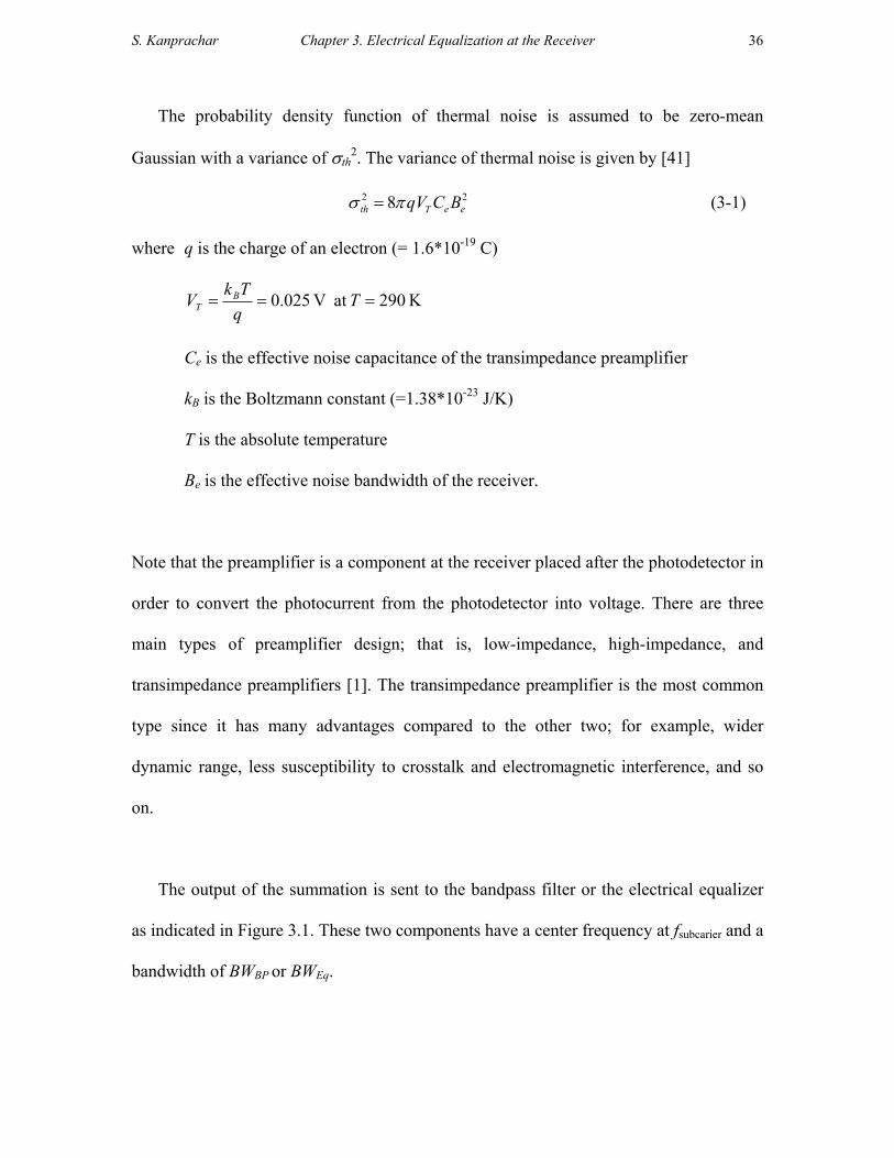
The block diagram for digital transmission with three subcarriers in the passband
region of the multimode fiber is shown in Figure 3.1. The input bit sequence from the bit
generator is sent through the pulse generator to generate the input pulses. The input pulse
is assumed to be a Gaussian shape with T0 = 0.25Tb, where T0 is the half-width at 1/e –
intensity point and Tb is the bit period. The spectrum of the input pulses is shifted to be
centered at the different subcarriers (fsubcarier). This signal is then passed through the laser
to convert the electrical signal into an optical signal. The spectrum of the complex
envelope of the optical signal contains the spectrum of the input pulses centered at fsubcarier
and an impulse with an amplitude of 1 located at f = 0 (this impulse is for the carrier
component of the light source). Passing this optical signal through the multimode fiber
(whose magnitude response is relatively flat at high frequencies), the spectrum of the
signal at high frequencies is attenuated. To limit the input optical power to a required
level, a variable attenuator (loss) is placed in front of the square-law detector. The optical
signal at the output of this attenuator is converted back to an electrical signal at the

S. Kanprachar Chapter 3. Electrical Equalization at the Receiver
35
square-law detector. The electrical output signal of the detector is combined with thermal
noise generated by the receiver (assuming that a PIN detector and transimpedance
amplifier receiver are used).
f
0 dB|HFiber(f)|
Multimode Fiber
LaserPulseGen
BitGen
fsub,1
Received signal at fsub,1
Atten-uator
Square-lawDetector
2
N thermal~ N (0,σth
2)
fsub,2
fsub,3
Demux forfsub,1
Demux forfsub,2
Demux forfsub,3
Received signalat fsub,2
Received signalat fsub,3
Combinedreceived signal
Bandpass filter
fGB P
BWBP
fsub,i
Lowpass filter
fG LP
BWLP
fsub, i
ElectricalEqualizer
f
BWE q
fsub,i
Demux for fsub, i
Figure 3.1 Diagram of the transmission system using three subcarriers on multimode fiber.
S. Kanprachar Chapter 3. Electrical Equalization at the Receiver
36
The probability density function of thermal noise is assumed to be zero-mean
Gaussian with a variance of σth2. The variance of thermal noise is given by [41]
2 28th T e eqV C Bσ π= (3-1)
where q is the charge of an electron (= 1.6*10-19 C)
K 290at V 025.0 === TqTkV B
T
Ce is the effective noise capacitance of the transimpedance preamplifier
kB is the Boltzmann constant (=1.38*10-23 J/K)
T is the absolute temperature
Be is the effective noise bandwidth of the receiver.
Note that the preamplifier is a component at the receiver placed after the photodetector in
order to convert the photocurrent from the photodetector into voltage. There are three
main types of preamplifier design; that is, low-impedance, high-impedance, and
transimpedance preamplifiers [1]. The transimpedance preamplifier is the most common
type since it has many advantages compared to the other two; for example, wider
dynamic range, less susceptibility to crosstalk and electromagnetic interference, and so
on.
The output of the summation is sent to the bandpass filter or the electrical equalizer
as indicated in Figure 3.1. These two components have a center frequency at fsubcarier and a
bandwidth of BWBP or BWEq.

S. Kanprachar Chapter 3. Electrical Equalization at the Receiver
37
Since the frequency response of the fiber is not known beforehand, it is necessary to
measure this response to adjust the equalizer. The response of the electrical equalizer for
each subcarrier channel is determined by sending narrowband noise as an input to the
multimode fiber at each subcarrier channel. At the receiver, this narrowband noise is
attenuated and shaped by the multimode fiber. To restore the narrowband noise to its
spectral shape at the input, the frequency response of the electrical equalizer must be the
inverse of the spectrum of the received narrowband noise. Hence, the frequency response
of the electrical equalizer can be determined from the received narrowband noise
spectrum. This process is done prior to transmitting the communication signal. The
output of the bandpass filter (or the electrical equalizer) is then passed through a mixer
and a lowpass filter. The output of the lowpass filter is the received signal, which is at
baseband. At the end of the diagram in Figure 3.1, it is seen that all received signals are
combined. This combination of the signals is done in order to study whether signal
quality can be improved if frequency diversity is used.
The plots of frequency responses of the multimode fiber and the input optical signals
at different fsubcarier, are shown in Figure 3.2. The frequency response of multimode fiber
is generated by taking the Fourier transform of the complex envelope of the impulse
response of multimode fiber, which is the combination of the delta functions
corresponding to different delays (see equation (2-1)). Each delay corresponds to a
particular guided mode supported by the multimode fiber. For this simulation, the
number of modes supported by the multimode fiber is 100 modes and the total delay
spread of the multimode fiber is 10 ns. Similarly, the frequency responses of three

S. Kanprachar Chapter 3. Electrical Equalization at the Receiver
38
subcarrier signals are generated by taking Fourier transform of the time responses of
three subcarrier signals. A bit rate (Rb) of each subcarrier signal is 50 Mbps. The bit rate
of 50 Mbps is used since it was found in Chapter 2 that the available bandwidth of each
passband of multimode fiber is approximately comparable to the intermodal bandwidth.
With a total delay spread of 10 ns, the intermodal bandwidth of the multimode fiber is
100 MHz. Consequently, the maximum bit rate for each subcarrier signal is then one-half
of that number; that is, 50 Mbps, since amplitude modulation of the subcarrier results in a
double sideband signal. The three subcarriers are taken to be at 0.5, 1.0, and 1.5 GHz to
illustrate different aspects of the effect of the fiber frequency response (see figure 3.2).
The gains of the bandpass and lowpass filters are assumed to be unity. The noise
equivalent bandwidth (prior to filtering) is assumed to be approximately equal to the
maximum subcarrier frequency plus Rb. Also, if the maximum subcarrier frequency is
very large compared to the bit rate (Rb), the noise equivalent bandwidth is then
approximated by the maximum subcarrier frequency. The effective noise capacitance (Ce)
of the receiver is taken to be 0.1 pF. Practical subcarrier receivers may have larger values
of Ce (see Chapter 8), but we are concerned in this chapter with relative rather than
absolute performance.

S. Kanprachar Chapter 3. Electrical Equalization at the Receiver
39
0 0.2 0.4 0.6 0.8 1 1.2 1.4 1.6 1.8 20
0.1
0.2
0.3
0.4
0.5
0.6
0.7
0.8
0.9
1
frequency (GHz)
Figure 3.2 Magnitude responses of multimode fiber and subcarrier signals located at 0.5, 1.0, and 1.5 GHz.
Considering the magnitude responses of the multimode fiber and the signals at
different subcarrier frequencies shown in Figure 3.2, it is seen that for the signal with
fsubcarier = 0.5 GHz, the magnitude response of the multimode fiber is very small (or a
null) at frequencies near 0.5 GHz. Hence, the subcarrier signal at this fsubcarier is strongly
attenuated. The equalizer then needs to provide high gain at this subcarrier frequency.
For the signals with fsubcarier = 1.0 and 1.5 GHz, there are no deep nulls located near the
main components (i.e., at fsubcarier and subcarrier bf R± ) of these subcarrier signals. The shapes
of the magnitude response of the multimode fiber from these two subcarriers are almost

S. Kanprachar Chapter 3. Electrical Equalization at the Receiver
40
identical except the amplitude. The amplitude of the multimode fiber at fsubcarier = 1.5
GHz is larger than at the amplitude of the multimode fiber at fsubcarier = 1.0 GHz.
The plots of eye-diagrams for different subcarrier frequencies are shown in Figure 3.3
to Figure 3.5. Also, the signal-to-noise ratios for the different cases are indicated on the
figures. The signal-to-noise ratio is determined by the ratio between the received signal
power and the noise power at the output of the lowpass filter. To get good performance,
the signal-to-noise ratio needs to be high since with this high signal-to-noise ratio, the
effect of noise on the decision between bit “0” and bit “1” is negligible; thus, a low bit-
error-rate is achieved. For a digital system, the signal-to-noise ratio is generally required
to be greater than 15 dB. The bandwidth of the bandpass filter (or the bandwidth of the
equalizer) is 4Rb. To show the improvement of frequency diversity, the eye-diagram of
the combined version of three received signals is given in Figure 3.5.
0 0.5 1 1.5 2 2.5 30
2
4
6x 10
−7
fsub = 0.5 GHzSNR
out =
16.21 dB
0 0.5 1 1.5 2 2.5 30
2
4
6
8x 10
−7
fsub = 1 GHzSNR
out =
16.36 dB
0 0.5 1 1.5 2 2.5 30
2
4
6
8x 10
−7
fsub = 1.5 GHzSNR
out =
20.25 dB
Time/Tb
Figure 3.3 Eye-diagrams of received subcarrier signals: without electrical equalization and BWBP = 4Rb.
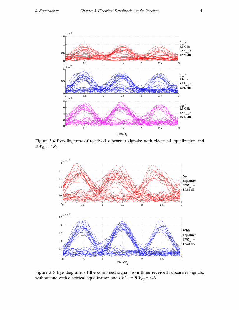
S. Kanprachar Chapter 3. Electrical Equalization at the Receiver
41
0 0.5 1 1.5 2 2.5 30
0.5
1
1.5x 10
−5
fsub = 0.5 GHzSNR
out =
12.26 dB
0 0.5 1 1.5 2 2.5 30
0.5
1x 10
−5
fsub = 1 GHzSNR
out =
13.67 dB
0 0.5 1 1.5 2 2.5 30
2
4
6
8x 10
−6
fsub = 1.5 GHzSNR
out =
15.12 dB
Time/Tb Figure 3.4 Eye-diagrams of received subcarrier signals: with electrical equalization and BWEq = 4Rb.
0 0.5 1 1.5 2 2.5 30
0.2
0.4
0.6
0.8
1x 10
−6
No Equalizer SNR
out =
15.61 dB
0 0.5 1 1.5 2 2.5 30
0.5
1
1.5
2
2.5x 10
−5
With Equalizer SNR
out =
17.78 dB
Time/Tb
Figure 3.5 Eye-diagrams of the combined signal from three received subcarrier signals: without and with electrical equalization and BWBP = BWEq = 4Rb.

S. Kanprachar Chapter 3. Electrical Equalization at the Receiver
42
From Figure 3.3 to Figure 3.5, it is seen that the output signal-to-noise ratio (SNRout)
depends mainly on the subcarrier frequency (i.e., the frequency response of the
multimode fiber at the particular subcarrier) and the type of modification used at the
receiver (i.e., without or with electrical equalization, frequency diversity).
Considering the effect of the subcarrier frequency, SNRout at fsubcarrier of 1.5 GHz is
higher than SNRout at fsubcarrier of 0.5 GHz. For example, from Figure 3.3, the values of
SNRout at fsubcarrier = 0.5, 1.0, and 1.5 GHz are 16.21, 16.36, and 20.25 dB, respectively.
This is explained by considering the magnitude response of the multimode fiber; that is,
the magnitude response of the multimode fiber in the vicinity of 0.5 GHz has a deep null
at 0.52 GHz and this null strongly attenuates the signal power at fsubcarrier = 0.5 GHz. On
the other hand, the magnitude response of the multimode fiber in vicinity of 1.5 GHz has
a good response and there is no deep null in this region. Thus, the output signal at this
subcarrier frequency has a good signal strength and hence large SNRout. Note that for the
subcarrier signal at fsubcarrier = 1.0 GHz even though there is no deep null at the frequency
component at 1.0 GHz, the attenuation from the multimode fiber at the component at
fsubcarrier ≤ Rb is larger than the attenuation from multimode fiber at the component at
fsubcarrier ≤ Rb for the subcarrier signal at fsubcarrier = 0.5 GHz. Hence, the SNRout of the
signal at fsubcarrier of 1.0 GHz is slightly larger than the SNRout of the signal at fsubcarrier 0.5
GHz.
The main difference between the cases of with and without equalization is the
response of the bandpass filter (used in the case of without equalization), which is flat,

S. Kanprachar Chapter 3. Electrical Equalization at the Receiver
43
and the response of the electrical equalizer, which depends on the frequency response of
the multimode fiber at a particular subcarrier frequency. This then results in a difference
between the signal-to-noise ratios from these two cases. It is seen from Figure 3.3 and 3.4
that the signal-to-noise ratio (SNRout,Eq) from the system with equalization is smaller than
the signal-to-noise ration (SNRout) from the system without equalization. Since the gain
profile of the electrical equalizer is not totally flat, the thermal noise at the frequency
which has a large gain can also be strongly enhanced. This then results in a larger thermal
noise power; thus, a small SNRout,Eq compared to SNRout. Hence, from this point, it is seen
that using an electrical equalizer does not significantly improve the system performance.
Combining three output signals from different subcarrier frequencies, that is, using
frequency diversity, might be a good way to reduce the receiver complexity since with
this diversity, the receiver does not need the ability to choose the best signal among
different subcarrier signals. For the case of without equalization, from Figures 3.3 and
3.5, it is seen that SNRout from the combined signal (i.e., 15.61 dB) is worse than SNRout
from the individual subcarrier frequency (i.e., 16.21, 16.36, and 20.25 dB from fsub = 0.5,
1.0, and 1.5 GHz, respectively). Thus, for the case of without equalization, combining the
output signals is not a good approach.
Considering the combined signal for the system with electrical equalization, a better
SNRout,Eq (compared to SNRout,Eq from the individual subcarrier frequency) can be
achieved. As given in Figure 3.4, SNRout,Eq from fsubcarrier of 0.5, 1.0, and 1.5 GHz are
12.26, 13.67, and 15.12 dB, respectively, while SNRout,Eq from the combined version
S. Kanprachar Chapter 3. Electrical Equalization at the Receiver
44
(from Figure 3.5) of these three signals is 17.78 dB. Comparing the combined signal for
the case of without equalization to the combined signal for the case of using equalization,
it is seen that SNRout for the case of without equalization is smaller. The reason for this is
explained in Appendix A. Note that the effect of the bandwidth of the bandpass filter (or
the bandwidth of the electrical equalizer) on the signal-to-noise ratio of the received
signal is also presented in Appendix A.
3.3 Signal-to-noise ratio and eye-diagram of the received signals: with limited-gain
electrical equalization
From the previous section, it is seen that using electrical equalization with three-
subcarrier system is not a good way to improve the signal quality since the signal-to-
noise ratio from such a system is small. This is the result of having large gain profile in
the response of the electrical equalizer; thus, noise is strongly amplified. To reduce the
noise amplification, the peak gain of the electrical equalizer has to be decreased. By
doing this, the amplitude of each subcarrier signal is not completely equalized but it is
interesting to determine whether the signal-to-noise ratio can be improved by limiting the
peak gain of the electrical equalizer.
In this section, the electrical equalizer is modified. As discussed, because of the
narrow-band high gain profile of the ideal electrical equalizer, noise is amplified

S. Kanprachar Chapter 3. Electrical Equalization at the Receiver
45
considerably. To limit this noise amplification, the gain of the electrical equalizer should
be limited. The illustration of the magnitude response of the ideal and limiter-gain
electrical equalizers is shown in Figure 3.6.
|HIdeal Eq ( f )|
Gmin
Gmax
0 f
|HLimited-gain Eq ( f )|
Gmin
0 f
∆G
Figure 3.6 Illustration of the magnitude response of the ideal and limited-gain equalizers
From the sketch, it is seen that for the ideal equalizer, there are two peaks. These two
peaks have large gain compared to the minimum gain of the ideal equalizer. Noise can be
enhanced significantly if it is passed through these regions. Thus, to limit the amount of
the noise amplification, the gain from these two peaks should be reduced. The maximum
difference between the minimum and maximum gains is needed and is abbreviated by
∆G. Applying ∆G to the ideal equalizer, the limited-gain equalizer is achieved and is also
shown in Figure 3.6. Note that the phase responses of these two equalizers are the same.
Using this limited-gain equalizer with the received signal, the eye diagrams and output
SNRs are shown in Figure 3.7 and 3.8.

S. Kanprachar Chapter 3. Electrical Equalization at the Receiver
46
0 0.5 1 1.5 2 2.5
1
2
3
4x 10
−6
fsub = 0.5 GHzSNR
out =
17.22 dB
0 0.5 1 1.5 2 2.5
2
4
6x 10
−6
fsub = 1 GHzSNR
out =
16.93 dB
0 0.5 1 1.5 2 2.5
2
4
6
x 10−6
Time/Tb
fsub = 1.5 GHzSNR
out =
21.27 dB
Figure 3.7 Eye-diagrams of received subcarrier signals: with limited-gain electrical equalization (∆G = 0 dB) and BWEq = 4Rb.
0 0.5 1 1.5 2 2.5
2
4
6
8
x 10−7
No Equalizer SNR
out =
16.63 dB
0 0.5 1 1.5 2 2.5
0.5
1
1.5
2
x 10−5
With Equalizer SNR
out =
18.24 dB
0 0.5 1 1.5 2 2.5
2468
101214
x 10−6
Time/Tb
With Equalizer(∆G =0 dB)SNR
out =
22.64 dB
Figure 3.8 Eye-diagrams of combined signal from three received subcarrier signals: for different cases, BWBP = BWEq = 4Rb.

S. Kanprachar Chapter 3. Electrical Equalization at the Receiver
47
Eye diagrams of the received signal with BWEq of 4Rb are shown in Figure 3.7. The
bandwidth of 4Rb is used since, as indicated in Appendix A, it results in less signal
distortion, although the signal-to-noise ratio from this large bandwidth is less than that
for smaller bandwidth. ∆G for the limited-gain equalizer used in Figure 3.7 and 3.8 is 0
dB; that is, the gain profile of the limited-gain equalizer is flat, only phase equalization is
performed. Considering the eye diagrams of individual subcarrier signals between the
limited-gain equalization in Figure 3.7 and ideal equalization in Figure 3.4, it is seen that
the eye opening of the limited-gain equalized signal is larger than the eye opening of the
ideal equalized signal. Also, the output SNR from the limited-gain equalized signal is
larger than the output SNR of the ideal equalized signal. This is the result of the gain
limiting in the limited-gain equalizer.
Combining the received signals, the eye diagrams of different cases are shown in
Figure 3.8. It is seen that the maximum eye opening and output SNR between three
combined signals are from the case of using limited-gain equalizer. This can be explained
as follows.
The reason of getting larger output SNR from the case of using ideal equalization
compared to the case of without equalization was discussed in the previous section. Here,
the reason of getting better output SNR from the case of using limited-gain equalization
compared to the case of using ideal equalization will be discussed. Since there is a
limitation on the gain profile of the limited-gain equalizer, noise from the case of using

S. Kanprachar Chapter 3. Electrical Equalization at the Receiver
48
limited-gain equalizer is then smaller than noise from the case of using ideal equalizer.
However, the phase response of the limited-gain equalizer is the same as the phase
response of the ideal gain equalizer. It means that the phases of the received subcarrier
signals for the case of using limited-gain equalizer are almost the same. Thus, combining
these signals will give an increase in signal power by approximately 9 dB, which is the
same as the increase achieved from the case of using the ideal equalizer. The total noise
power is just the linear summation of noises from different equalized signals. It is seen
that the increase of the output SNR of the combined signal for the case of using limited-
gain equalization is the same as that for the case of using ideal equalization. However,
since the output SNR from individual limited-gain equalized signal is better than the
output SNR from individual equalized signal, the output SNR of the combined signal from
the case of using limited-gain equalizer is then larger than that from the case of using
ideal equalizer as seen from Figure 3.8.
From this section, it is seen that limiting the maximum gain of the equalizer will
improve the output SNR of individual subcarrier signal since thermal noise is not strongly
amplified. Moreover, it is shown from Appendix B that the best output SNR is achieved
from using phase equalization (∆G = 0 dB). Combining the equalized signals can
increase the output SNR. The achieved output SNR depends on many factors; that is, the
magnitude response of the multimode fiber at particular subcarrier frequency, the
bandwidth of the equalizer, the maximum difference between the minimum and
maximum gains (∆G), and the type of the signal (individual or combined).

S. Kanprachar Chapter 3. Electrical Equalization at the Receiver
49
3.4 Comparisons of Signal-to-noise ratio and eye-diagram from different cases
The simulation results of sending a signal using three subcarriers on multimode fiber
have been presented. It has been seen that the quality of received subcarrier signal
depends on many factors; the frequency response of the multimode fiber at a particular
subcarrier channel, the bandwidth of the bandpass filter (or the bandwidth of the
electrical equalizer), and type of equalization used in the system.
If the subcarrier is located at or near a deep null of the magnitude response of the
multimode fiber, the received signal from that subcarrier will be significantly attenuated.
Hence, the signal-to-noise ratio of the received signal will be very low. The bandwidth of
the bandpass filter (or the bandwidth of the electrical equalizer) is also another factor
determining the quality of the received signal. If this bandwidth is too small, the high
frequency components of the signal are rejected and not included in the received signal.
This then results in degradation on the shape and power of the received signal. However,
with large bandwidth, more noise is included in the signal; thus, a lower signal-to-noise
ratio is achieved.
Adding ideal electrical equalization to the receiver helps improve the shape of the
received signal as seen from Figure 3.3 and 3.4. However, since it is not just the signal
that passes through the ideal electrical equalizer, noise also passes through this
component; the gain profile (which is not flat) of the equalizer can intensify the noise
power significantly. This leads to strong noise at the output of the equalizer; thus, low

S. Kanprachar Chapter 3. Electrical Equalization at the Receiver
50
signal-to-noise ratio. If the maximum gain of the equalizer is limited, the noise
intensification can be reduced. It is shown that using limited-gain electrical equalizer can
increase the signal-to-noise ratio of the received signal, and the best result is obtained by
using a phase equalizer.
Applying frequency diversity to the system by combining all three received signals
might be a good way to reduce the system complexity at the receiver since there is no
need to have a circuit to choose the best received signal. It is shown that for the case of
combined signals without equalization the signal-to-noise ratio is actually lower than that
of the individual received signals. On the other hand, the quality of the combined signal
for the case with electrical equalization (both ideal and limited-gain equalization) is
improved; especially, for the case with limited-gain equalization, the signal-to-noise ratio
of the combined signal is at least 2 dB higher than the highest signal-to-noise ratio among
the three received signals (see Appendix B).
3.5 Conclusions
It is shown that transmitting a signal using high frequency region of multimode fiber
is possible. The quality of the received signal depends mainly on the magnitude response
of the multimode fiber at the particular subcarrier channel. Using just ideal electrical
equalization does not improve anything. It, moreover, can degrade the received signal by
enhancing the noise power; thus, lowering the signal-to-noise ratio. On the other hand,

S. Kanprachar Chapter 3. Electrical Equalization at the Receiver
51
using a phase equalizer can improve the received signal quality since it does not increase
the noise power. And, the received signal can be further improved if all received signals
are combined.
The problem of using equalization is that the system needs to know the properties of
all subcarrier channels in advance so that the frequency response of the equalizer can be
constructed. These properties may need to be updated frequently if the properties of these
subcarrier channels are time-varying. And, if, for higher bit rate transmission, the number
of transmitted signals increases, the number of equalizers has to be increased; thus, more
system complexity is added. Also, it is shown that the signal-to-noise ratio of the
received signal from the system with phase equalization is not much different from the
signal-to-noise ratio from the received signal from the system without equalization.
Although combining the received signals with phase equalization will help improve the
signal quality it is not bandwidth-efficient and cost-efficient since three bandpass regions
and three subcarrier systems are used for transmitting just one signal. Therefore, adding
electrical equalization to the receiving end is not a suitable choice for improving the
signal transmission using the bandpass region of multimode fiber.

S. Kanprachar Chapter 4. Spread Spectrum with Multimode Fiber System
52
Chapter 4
Spread Spectrum with Multimode Fiber System
4.1 Introduction
Adding electrical equalization to the receiving end of bandpass transmission on a
multimode fiber does not improve the received signal quality, as shown in Chapter 3. The
signal-to-noise ratio of the received signal is degraded since the noise is significantly
amplified by the equalizer. However, it was shown that combining all phase-equalized
signals can improve the quality of the received signal. This means that to transmit a
narrowband signal, frequency diversity and phase equalization are needed. Using
equalization with a multimode fiber system may not be practical since if the channels are
time-varying, the equalizers may need to be updated frequently to correctly equalize the
received signals. This then adds more complexity to the system. However, it might be
possible to improve performance by spreading the spectrum of the signal over a
bandwidth larger than the correlation bandwidth of the channel thereby obtaining the
effect of frequency diversity. Even if there is a frequency component located at a null, the
degradation from such null to the overall received signal should be small.
S. Kanprachar Chapter 4. Spread Spectrum with Multimode Fiber System
53
In this chapter, we consider the case where the spectrum of the transmitted signal is
spread out. This spread spectrum signal modulates a subcarrier and is then sent through
the multimode fiber. The eye-diagram and signal-to-noise ratio of the received signal are
determined and compared to the case of not using spread spectrum. The simulation of the
probability density function and cumulative distribution of the signal-to-noise ratio of the
received signal from the system without and with spread spectrum are presented.
4.2 Signal-to-noise ratio and eye-diagram
The block diagram of a transmission system using spread spectrum with a subcarrier
signal is shown Figure 4.1. The spectrum of the input signal is spread by using the direct
sequence (DS) technique. The input signal is multiplied by a code sequence, c(t). The
code sequence, c(t), is generated by using pseudo-noise sequence generation. The code
generator contains an N-stage shift register and mod-2 addition. The code length depends
on the number (N) of stages in the shift register; that is, code length = 2N –1. The pulse
width (Tc) of the code sequence is much smaller than the bit period (Tb) of the input
signal and the ratio between the bit period of the input signal and the pulse width of the
code sequence equals the code length (or 2N –1). Thus, multiplying the input signal with
this code sequence, the bandwidth of the spread spectrum signal is equal to (2N –1)×Rb.
Detailed information about spread spectrum systems can be found in [37 – 39].
After multiplying the input signal with the code sequence, the center of the spread
spectrum signal is shifted to a high frequency; that is, to the subcarrier frequency
(fsubcarrier). This subcarrier spread spectrum signal is converted to an optical format by the

S. Kanprachar Chapter 4. Spread Spectrum with Multimode Fiber System
54
laser, and is transmitted through the bandpass region of the multimode fiber system. At
the receiver, the received optical signal is detected and converted back to an electrical
signal. Thermal noise is added to the signal at this point. The assumption for thermal
noise is the same as used in Chapter 2. The signal is passed through a bandpass filter to
filter out both the DC and high frequency components. The center frequency of this
bandpass spread spectrum signal is shifted to zero frequency by multiplying with the
subcarrier frequency. After that, the spread spectrum signal is decoded by multiplying
with c(t) and passed through a lowpass filter to filter out the unwanted high frequency
components, thereby recovering the received baseband signal.
f
0 dB|HFiber(f)|
Multimode Fiber
LaserPulseGen
BitGen
fsubcarrier
ReceivedSignal
Bandpass filter
fGBP
BWBP
fsub
Square-lawDetector
2
Lowpass filter
fGLP
BWLP
fsubcarrierNthermal ~ N (0,σth2)
Atten-uator
(L)
c(t)
c(t)
Figure 4.1 Diagram of the transmission system using subcarrier frequency and direct sequence spread spectrum within the passband region of the multimode fiber.

S. Kanprachar Chapter 4. Spread Spectrum with Multimode Fiber System
55
0 0.2 0.4 0.6 0.8 1 1.2 1.4 1.6 1.80
0.2
0.4
0.6
0.8
1
frequency (GHz)
Input signalMultimode fiber
0 0.2 0.4 0.6 0.8 1 1.2 1.4 1.6 1.80
0.2
0.4
0.6
0.8
1
frequency (GHz)
Coded input signalMultimode fiber
Figure 4.2 Magnitude responses of the multimode fiber, the input signal, and the input spread spectrum (code length = 7) signal: First simulation.
0 0.5 1 1.5 2 2.5 30
0.5
1
1.5
2
2.5x 10
−6
No SSSNR = 21.4 dB
Time/Tb
0 0.5 1 1.5 2 2.5 30
0.5
1
1.5
2
2.5x 10
−6
With SS G
coding =7
SNR = 19.6 dB
Time/Tb
Figure 4.3 Eye-diagrams of the received signal in the first simulation: without and with spread spectrum (code length = 7).

S. Kanprachar Chapter 4. Spread Spectrum with Multimode Fiber System
56
0 0.2 0.4 0.6 0.8 1 1.2 1.4 1.6 1.80
0.2
0.4
0.6
0.8
1
frequency (GHz)
Input signalMultimode fiber
0 0.2 0.4 0.6 0.8 1 1.2 1.4 1.6 1.80
0.2
0.4
0.6
0.8
1
frequency (GHz)
Coded input signalMultimode fiber
Figure 4.4 Magnitude responses of the multimode fiber, the input signal, and the input spread spectrum (code length = 7) signal: Second simulation.
0 0.5 1 1.5 2 2.5 30
1
2
3
4
5
6x 10
−7
No SSSNR = 9.6 dB
Time/Tb
0 0.5 1 1.5 2 2.5 30
0.2
0.4
0.6
0.8
1
1.2x 10
−6
With SS G
coding =7
SNR = 14.9 dB
Time/Tb
Figure 4.5 Eye-diagrams of the received signal in the second simulation: without and with spread spectrum (code length = 7).

S. Kanprachar Chapter 4. Spread Spectrum with Multimode Fiber System
57
Using the diagram shown in Figure 4.1, the simulation is done for two trials (i.e., two
sets of multimode fiber) with the code length of 7. This code length is from a code
generator containing 3 shift-registers. With an input bit rate (Rb) of 50 Mbps, the total
bandwidth of the spread spectrum signal equals 7×2×Rb = 700 MHz. The total delay
spread from different guided modes in the multimode fiber considered here is 10 ns;
hence, the correlation bandwidth of the fiber is approximately 100 MHz. It is seen that
the total bandwidth of the spread spectrum signal is 7 times larger than this correlation
bandwidth. Other important parameters used in the simulation are given as follows: BWBP
= 4Rb, BWLP = 2Rb, fsub = 1.5 GHz. The magnitude response of the multimode fiber, the
input signal, and the spread-spectrum signal are presented in Figures 4.2 and 4.4. Also,
the eye-diagram of the received signal and the achieved signal-to-noise ratio are shown in
Figures 4.3 and 4.5.
From Figure 4.2 to 4.5, it is seen that the performance of the received signal depends
mainly on the magnitude response of the multimode fiber and the type of the signal (with
or without spread spectrum). That is, if the subcarrier signal is located at the middle of
the passband region, the achieved SNR will be large (as seen from the first simulation).
However, if the subcarrier signal is at the null region of the response of the multimode
fiber (not at the middle of the passband), the achieved SNR then becomes small (as seen
from the second simulation). In the first simulation, the output SNR in the case of spread
spectrum (SNRout,ss) is slightly smaller than the corresponding quantity in the absence of
spread spectrum (SNRout) since the high frequency signal of the spread spectrum signal is
attenuated by the multimode fiber response (~ 1.7 GHz). However, from the second

S. Kanprachar Chapter 4. Spread Spectrum with Multimode Fiber System
58
simulation, it is seen that SNRout is smaller than SNRout,ss since the magnitude response of
multimode fiber at the frequency of 1.5 GHz is very poor. Spreading the spectrum of the
input signal can lessen the effect of the poor response at the frequency of 1.5 GHz.
Comparing the two simulations, it is seen that as the magnitude response of the
multimode fiber varies, the variation of achieved SNR for the case of using spread
spectrum with the transmit signal is smaller than the variation of the SNR for the case of
not using spread spectrum; that is, ∆SNRout,ss = 4.7 dB < 11.8 dB = ∆SNRout.
Considering the eye diagram from the first simulation in Figure 4.3, it is seen that the
shape of the eye diagram for the case of not using spread spectrum is better than that
when spread spectrum is used. This may be explained as follows. For the case when
spread spectrum is used, the amplitude of the high frequency component (greater than Rb)
of the received signal may be large (depending on the magnitude response of the fiber).
And, if the bandwidth of the lowpass filter covers this high frequency range, the received
signal amplitude spectrum is distorted which results in a distortion of the pulse shape. In
this simulation the bandwidth of the lowpass filter equals 2Rb. If the bandwidth of the
lowpass filter is decreased to 1.5Rb, the shape of the achieved eye diagram should be
improved since the frequency component at 2Rb, which can be large, is not included. For
the second simulation in Figure 4.5, the same explanation can be used. However, since
the magnitude response of the multimode fiber in this simulation is very poor in the
vicinity of the frequency of 1.5 GHz, the eye-diagram of the received signal from the
system without spread spectrum is degraded significantly as seen from the figure.

S. Kanprachar Chapter 4. Spread Spectrum with Multimode Fiber System
59
4.3 Probability density function of signal-to-noise ratio
The previous simulations suggest that the variation of SNR from the system with
spread spectrum is smaller than the variation of SNR from the system without spread
spectrum. However, this conjecture is only from two simulations. More simulations are
required to understand this variation.
In this section, the probability density function of the received SNR is studied using
computer simulation. Two types of systems are studied; that is, without and with spread
spectrum. The received SNR of each system is collected. There are 300 simulations for
each system. The histograms of the received SNR from both systems are shown. The
average SNR, the standard deviation, and the difference between maximum and minimum
SNR are determined. There are two cases for the system using spread spectrum; that is,
with code lengths of 7 and 15. The bandwidths of the spread spectrum signal from these
two cases are equal to 7BWcorr and 15BWcorr, where BWcorr is the correlation bandwidth of
multimode fiber at high frequencies. Other parameters used in Figure 3.2 to Figure 3.5
are also used in this section.

S. Kanprachar Chapter 4. Spread Spectrum with Multimode Fiber System
60
0 5 10 15 20 25 300
20
40
60No spread spectrum SNR
max−SNR
min = 22.3 dB
<SNR> = 17 dBσ
SNR = 4.1 dB
0 5 10 15 20 25 300
10
20
30
40
50With spread spectrumG
coding = 7
SNRmax
−SNRmin
= 19.6 dB<SNR> = 14 dBσ
SNR = 3.1 dB
0 5 10 15 20 25 300
20
40
60With spread spectrumG
coding = 15
SNRmax
−SNRmin
= 14.5 dB<SNR> = 11.3 dBσ
SNR = 2.4 dB
SNRoutput (in dB)
Figure 4.6 Histogram of the signal-to-noise ratio from 300 simulations: without and with spread spectrum (code length of 7 and 15).
In Figure 4.6, the histograms of the received SNRs from the case of not using spread
spectrum and from the case of using spread spectrum with code length of 7 and 15 are
shown. Considering these histograms, it is seen that the shapes of the histograms are
similar to a Gaussian shape, especially for the cases using spread spectrum. The shape of
the histogram of the system without spread spectrum is asymmetric with a long tail at low
SNR. Considering the data given in these plots, it is seen that the difference between the
maximum and the minimum SNRs for the case of using spread spectrum (i.e., 19.6 dB
and 14.5 dB for the code length of 7 and 15, respectively) is smaller than that from the
case of not using spread spectrum (i.e., 22.3 dB). The standard deviations of the case with
spread spectrum with code length of 7 and 15 are 3.1 dB and 2.4 dB, respectively. These

S. Kanprachar Chapter 4. Spread Spectrum with Multimode Fiber System
61
standard deviations are smaller than the standard deviation of the case without spread
spectrum, which is 4.1 dB. It is seen that the achieved SNR from the system with spread
spectrum has a smaller variation. The reason for getting smaller variation of SNR from
the system with spread spectrum may be explained as follows. Multiplying the
transmitted signal with a pseudo-random sequence with a pulse width much smaller than
the bit period, the spectrum of the transmitted signal is spread out and covers more
passband regions of the multimode fiber. It has been shown that for this high frequency
range, the average of the magnitude response of the multimode fiber depends mainly on
the number of guided modes. However, if a narrowband signal is sent through this
passband region, there is no guarantee that it will always be located at the middle of the
passband region; thus, large variance of the achieved SNR results. To lower the risk of
putting the signal spectrum at any possible null of the fiber magnitude response, the
signal spectrum should be large enough to cover many passband regions. Although more
nulls are included, on the average, there is less variation of the magnitude response, and
consequently less variation of the achieved SNR. However, it is seen that the average SNR
from the case with spread spectrum is smaller than the average SNR from the case
without spread spectrum; for example, <SNRavg,SS,CL=7> = 14 dB < 17 dB = <SNRavg,No
SS>. This can be explained by considering the receiving end of the system. It is seen that
at the receiver, the received optical signal is converted to an electrical signal by a square-
law detector, as seen in Figure 4.1. The phase information of the received optical signal is
not included in the electrical signal. Hence, when this spread spectrum electrical signal is
decoded by multiplying with the code sequence, c(t); the spectra of this signal from
different frequencies are combined. However, since the phase information of the received

S. Kanprachar Chapter 4. Spread Spectrum with Multimode Fiber System
62
optical signal is not included, there is no guarantee that these spectra are in-phase. That
is, combining these spectra does not necessarily increase, but may decrease, the power of
the decoded signal. And, when these spectra are combined, the noise components from
these spectra are also combined. The output noise power is just the linear sum of the
noise powers from different spectra. And, if the number of spectra increases (i.e., the
code length increases), the output noise power becomes larger. It is seen that the power of
the decoded signal does not increase while the output noise power increases linearly as a
function code length; hence, the average SNR of the received signal from the spread
spectrum system decreases as the code length increases. Consequently, the average SNR
of the received signal from the system with spread spectrum is smaller than the average
SNR of the received signal from the system without spread spectrum.
Considering the histograms from the system with spread spectrum with code length of
7 and 15, it is seen that the received SNR from the case of code length of 15 is better that
the received SNR from the case of code length of 7 in terms of the difference between the
maximum and the minimum SNR and the standard deviation of the received SNR.
However, there is a disadvantage of using large code length. That is, with the larger code
length, the average SNR is smaller. Also, with larger code length, the spectrum of the
spread spectrum signal is larger; that is, more bandpass bandwidth is needed.
From the histograms shown in Figure 4.6, it is interesting to determine the cumulative
distribution of the SNR for different cases. Using the cumulative distribution, the
probability that the received signal is higher than a particular required SNR, can be

S. Kanprachar Chapter 4. Spread Spectrum with Multimode Fiber System
63
determined. The data used in Figure 4.6 is used to generate three plots of the cumulative
distribution for the case of without and with spread spectrum (code length of 7 and 15),
as presented in Figure 4.7.
0 5 10 15 20 25 300
0.2
0.4
0.6
0.8
1
FS
NR(S
NR) No spread spectrum
SNRmax
−SNRmin
= 22.3 dB<SNR> = 17 dBσ
SNR = 4.1 dB
0 5 10 15 20 25 300
0.2
0.4
0.6
0.8
1
FS
NR(S
NR)
With spread spectrumG
coding = 7
SNRmax
−SNRmin
= 19.6 dB<SNR> = 14 dBσ
SNR = 3.1 dB
0 5 10 15 20 25 300
0.2
0.4
0.6
0.8
1
SNRoutput (in dB)
FS
NR(S
NR)
With spread spectrumG
coding = 15
SNRmax
−SNRmin
= 14.5 dB<SNR> = 11.3 dBσ
SNR = 2.4 dB
Figure 4.7 Cumulative distribution of signal-to-noise ratio from 300 simulations: without and with spread spectrum (code length of 7 and 15).
From Figure 4.7, it is clearly seen that the cumulative distribution function of the case
without spread spectrum is better than that from the case of with spread spectrum. And,
the cumulative distribution function from the spread spectrum system with small code
length is better that from the spread spectrum system with large code length. For
example, if the required SNR is 15 dB, it can be approximated from Figure 4.7 that

S. Kanprachar Chapter 4. Spread Spectrum with Multimode Fiber System
64
P{SNRNo SS ≤ 15 dB} = 0.25
P{SNRSS, code length = 7 ≤ 15 dB} = 0.62
P{SNR SS, code length = 15 ≤ 15 dB}= 0.95.
From these probabilities, it is seen that spread spectrum is not a good way to transmit
a signal using the bandpass region of multimode fiber since the probability of having the
achieved SNR less than a required SNR from the system with spread spectrum is larger
than the probability from the system without spread spectrum. And, this probability
increases as the code length increases.
4.4 Conclusions
The signal transmission using spread spectrum with multimode fiber system has been
simulated, and the eye-diagrams and the SNR from the system without and with spread
spectrum have been presented. It is seen that the received signal quality depends mainly
on the magnitude response of the multimode fiber. Using direct sequence spread
spectrum can improve the quality of the received signal if the subcarrier is located in
vicinity of a null, as seen from Figure 4.5. However, if the subcarrier is not located in
vicinity of a null, applying spread spectrum technique to the system may degrade the
quality of the received signal since the spread spectrum signal will cover a larger
bandwidth including more variation in the frequency response. The probability density
function and the cumulative distribution of the received SNR for the systems without and

S. Kanprachar Chapter 4. Spread Spectrum with Multimode Fiber System
65
with spread spectrum are also determined numerically from 300 simulations. The SNR of
the spread spectrum system is better than the SNR of the system without spread spectrum
in terms of the variation in the SNR and the difference between the maximum and
minimum SNR. However, the average SNR from the case with spread spectrum is smaller
than the average SNR from the case without spread spectrum. For the system with spread
spectrum, a larger code length system results in a smaller variation of the SNR and a
smaller difference between the maximum and minimum SNR. But, with a large code
length, the average SNR becomes smaller. This is because the square-law detector does
not provide coherent addition of the different frequency components of the signal. Using
the plots of cumulative distribution in Figure 4.7, it is clearly seen that spread spectrum is
not a good approach to transmit the signal using the bandpass region of multimode fiber
since the probability of having the received SNR less than a required SNR from the
system with spread spectrum is much larger than that from the system without spread
spectrum. In conclusion, direct sequence spread spectrum is not a good technique to
improve the performance of the bandpass transmission on multimode fiber.

S. Kanprachar Chapter 5. Subcarrier Multiplexing with Multimode Fiber System
66
Chapter 5
Subcarrier Multiplexing with Multimode Fiber System
5.1 Introduction
The effects of using electrical equalization and spread spectrum with bandpass
transmission on multimode fiber have been considered in Chapters 3 and 4, respectively.
Adding electrical equalization to the receiving end does not improve the system
performance since noise amplification is very strong and it results in a small signal-to-
noise ratio (SNR). For the spread spectrum system, the variation of the received SNR has
been shown to be smaller than that for a system without spread spectrum. However,
spread spectrum reduces the average received SNR and the reduction is larger as the
spread factor increases. Therefore, neither electrical equalization at the receiver nor direct
sequence spread spectrum improves the performance of bandpass transmission on
multimode fiber. Hence, another approach must be considered.
To transmit a high bit rate signal over the high frequency region of multimode fiber,
where the magnitude response is relatively flat (as analyzed in Chapter 2), dividing the

S. Kanprachar Chapter 5. Subcarrier Multiplexing with Multimode Fiber System
67
high bit rate signal into many low bit rate signals and modulating these low bit rate
signals onto different subcarriers might be a good technique. As discussed in Chapter 1,
instead of sending a high bit rate signal through one subcarrier, transmitting many low
data rate signals through different subcarriers, the wideband frequency-selective channel
can be changed into a series of narrowband frequency-nonselective channels. Hence, the
amplitude variation of each subcarrier channel is much less than the amplitude variation
from one wideband subcarrier channel. This technique is similar to the Orthogonal
Frequency Division Multiplexing (OFDM), which is now being widely considered in
wireless communications systems in order to overcome the effects of having a wideband
frequency-selective channel. However, in OFDM, all subcarriers are stacked tightly
because of bandwidth limitations. This is of smaller concern in bandpass transmission on
multimode fiber since the bandpass bandwidth of multimode fiber is very large; hence,
there is no need to stack all subcarriers tightly as done in OFDM.
In this chapter, consideration is given to the transmission of a high bit rate signal
through a multimode fiber system using subcarrier multiplexing (SCM). This high bit rate
signal is divided into Ncarrier small bit rate signals, where Ncarrier is the number of
subcarriers used in the SCM system. The bit-error-rate (BER) of the SCM system for
different numbers of subcarriers and different sets of multimode fiber is determined, and
the effect of the number of subcarriers on the achieved BER is discussed.

S. Kanprachar Chapter 5. Subcarrier Multiplexing with Multimode Fiber System
68
5.2 Bit-error-rate of the received signal for a 20-subcarrier SCM multimode fiber
system
fsub,1
BitGen S/P
PulseGen
PulseGen
PulseGen
fsub,2
fsub,Ncarrier
Laser
f
0 dB|HFiber(f)|Multimode Fiber
Atten-uator
(L)
Rb
Rb,SCM=RbNcarrier
ReceivedSignal
Nthermal~ N(0,σth
2)
fGBP
BWBP
fsub,2
Bandpass filter
fGBP
BWBP
fsub,1
fGBP
BWBP
fsub,Ncarrier
fsub,1
fsub,2
fsub,Ncarrier
Lowpass filter
fGLP
BWLP
fGLP
BWLP
fGLP
BWLP
SCMsignal
at fsub,1
SCMsignalat fsub,2
SCMsignal
at fsub,Ncarrier
P/S
Rb
Rb,SCM=RbNcarrier
DecisionCircuit
DecisionCircuit
DecisionCircuitSquare-law
Detector2
Figure 5.1 Diagram of the multimode fiber transmission using subcarrier multiplexing (SCM).
A block diagram of the system considered is given in Figure 5.1. The input bits from
a high bit rate signal are divided into Ncarrier blocks at the serial-to-parallel block, where
Ncarrier is the number of subcarriers in the system. The total bit rate is Rb and the bit rate
of each subcarrier signal is Rb,SCM (=Rb/Ncarrier). Each SCM bit stream is passed through a
pulse shaping block and then passed through a frequency mixer to modulate the signal
with the desired subcarrier frequency. The subcarrier signals are combined and sent to the
laser transmitter. The composite signal current, which intensity modulates the laser, is
given by [34]
S. Kanprachar Chapter 5. Subcarrier Multiplexing with Multimode Fiber System
69
( ) ( )1
1 coscarrierN
bias i ii
I t I m tω=
= +
∑ (5-1)
where Ibias is the bias current, which must be larger than the threshold current (Ith)
of the laser in order to operate the laser in the stimulated emission region;
mi is the modulation index corresponding to the ith subcarrier signal and is
defined by the ratio of the amplitude of the ith subcarrier signal to the
difference between the bias current and the threshold current [1]; that is,
ii
bias th
ImI I∆
=−
(5-2)
ωi is the angular subcarrier frequency corresponding to the ith subcarrier
signal
The output optical power of the laser is given by
( ) ( ),1
1 coscarrierN
T Optical o i ii
P t P m tω=
= +
∑ (5-3)
where Po is the optical output power when there is no signal.
From (5-3), the average and variance of the output optical power are given by
( ),T Optical oP t P= (5-4)
and, 2
2 2
12
carrierNo
Optical ii
P mσ=
= ∑ (5-5)
If the modulation index of each subcarrier signal is assumed to be the same; that is, mi =
m, the variance of the output optical power is then given by

S. Kanprachar Chapter 5. Subcarrier Multiplexing with Multimode Fiber System
70
2 2
2
2o carrier
OpticalP m Nσ = (5-6)
From (5-4) and (5-6), the total rms modulation index, µ, of the optical signal is
defined by
2
2 2Optical carrier
o
NmP
σµ = = (5-7)
The total rms modulation index is the parameter that determines the nonlinear
distortion. If the total rms modulation index is too large, there will be a significant
probability that the drive current to the laser will fall below threshold which will result in
clipping of the negative peaks of the input SCM signal. This, in turn, will lead to
nonlinear distortion. As shown in [34 - 36], if the total rms modulation index is not
greater than 0.5 then the carrier to nonlinear distortion ratio is greater than 25 dB which is
sufficient for a digital system. Hence, in the simulation, µ = 0.5 is used. A Gaussian pulse
shape is used in the simulation with an rms width T0 = 0.25Tb,SCM. The subcarrier signals
are combined and sent to the laser transmitter. The optical signal is passed through a
multimode fiber and an attenuation block that controls the input optical power (Pr,opt) to
the square-law photodetector having a responsivity of 0.9 mA/mW. Noise is added to the
signal at the output of the photodetector, the power (i.e., the variance, 2thσ ) of which is
proportional to the noise equivalent bandwidth of the receiver. For all simulations in this
chapter and following chapters, the noise equivalent bandwidth is 8 GHz and the rms
thermal noise current (referred to the output of the photodtector) is 0.8 µA, which is
determined from (3-1) in Chapter 3 with Ce = 0.1 pF. It should be noted that the noise
equivalent bandwidth is not critical since the receiver noise is limited by the electrical

S. Kanprachar Chapter 5. Subcarrier Multiplexing with Multimode Fiber System
71
filtering. The output of the square-law photodetector including noise is divided into
Ncarrier paths. The signal in the ith path is sent to a bandpass filter, whose center frequency
is located at the ith subcarrier frequency (where i = 1, 2, …, Ncarrier) to filter out all other
subcarrier signals. The filtered subcarrier signal is passed through a frequency mixer and
a lowpass filter to demodulate the signal to baseband and to further reject out of band
noise. Each subcarrier baseband signal is sent to a decision circuit to recover the output
subcarrier bit stream. Then, all subcarrier bit streams are combined to obtain the received
serial bit stream.
Simulations are done for 5 different sets of multimode fiber with 100 guided modes,
whose magnitude responses are shown in Figure 5.2. The delay spread and average delay
are 10 ns and 5 µs, respectively. The transmission bandwidth used in the simulation is
from 4.25 GHz to 7.5 GHz.
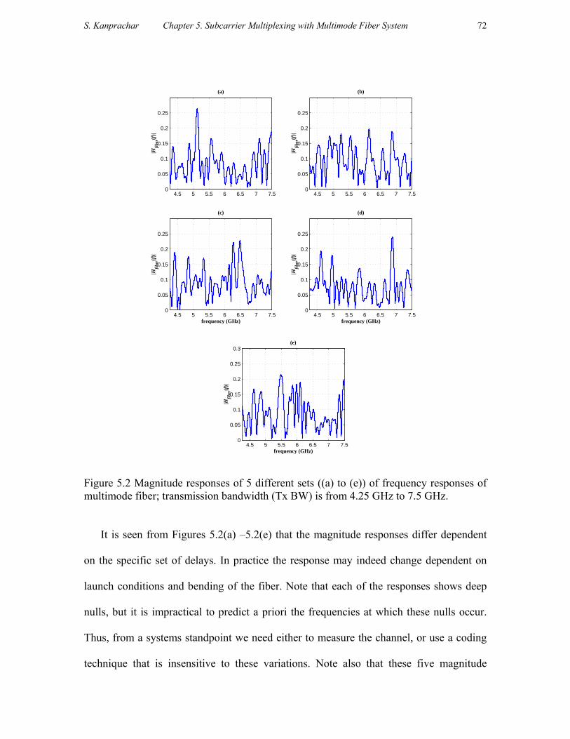
S. Kanprachar Chapter 5. Subcarrier Multiplexing with Multimode Fiber System
72
4.5 5 5.5 6 6.5 7 7.50
0.05
0.1
0.15
0.2
0.25
|Hfi
ber(f
)|
(a)
4.5 5 5.5 6 6.5 7 7.50
0.05
0.1
0.15
0.2
0.25
|Hfi
ber(f
)|
(b)
4.5 5 5.5 6 6.5 7 7.50
0.05
0.1
0.15
0.2
0.25
|Hfi
ber(f
)|
frequency (GHz)
(c)
4.5 5 5.5 6 6.5 7 7.50
0.05
0.1
0.15
0.2
0.25
|Hfi
ber(f
)|
frequency (GHz)
(d)
4.5 5 5.5 6 6.5 7 7.50
0.05
0.1
0.15
0.2
0.25
0.3
|Hfi
ber(f
)|
frequency (GHz)
(e)
Figure 5.2 Magnitude responses of 5 different sets ((a) to (e)) of frequency responses of multimode fiber; transmission bandwidth (Tx BW) is from 4.25 GHz to 7.5 GHz.
It is seen from Figures 5.2(a) –5.2(e) that the magnitude responses differ dependent
on the specific set of delays. In practice the response may indeed change dependent on
launch conditions and bending of the fiber. Note that each of the responses shows deep
nulls, but it is impractical to predict a priori the frequencies at which these nulls occur.
Thus, from a systems standpoint we need either to measure the channel, or use a coding
technique that is insensitive to these variations. Note also that these five magnitude

S. Kanprachar Chapter 5. Subcarrier Multiplexing with Multimode Fiber System
73
responses are chosen such that poor responses are included. The intent here is to consider
“near worst case” conditions. The extent to which this is so will be analyzed in
subsequent chapters
-BER calculation
In principle, the BER of each subcarrier signal could be determined by Monte Carlo
simulation with random noise. However, for very low BER, this would take too much
time since we have to generate many bits in order to get just one bit error. And, if more
BER precision is required, only one bit error is not enough. Thus, a semi-analytic
approach is adopted where the signal-to-noise ratio and a quantity called the Q-parameter
are determined by simulation, and then analytic formulas relating the Q-parameter to
error probability are used. This, in effect, assumes that the noise at the decision circuit is
Gaussian distributed, which is a good assumption for the PIN receiver model considered
here. The Q-parameter is calculated as follows [33].
The BER of each subcarrier signal is given by
[1] [0 |1] [0] [1| 0]SCMBER P P P P= + (5-8)
where P[1] = probability of sending bit 1
P[0] = probability of sending bit 0
P[0|1] = probability of deciding bit 0 when bit 1 is sent
P[1|0] = probability of deciding bit 1 when bit 0 is sent.

S. Kanprachar Chapter 5. Subcarrier Multiplexing with Multimode Fiber System
74
Assuming that bit 1 and bit 0 are equally likely to be sent, P[1] = P[0] = 1/2 and
BERSCM is given by
[ ]1 [0 |1] [1| 0]2SCMBER P P= + (5-9)
P[0|1] and P[1|0] depend on the probability density functions of bit 1 and bit 0 at the
input of the decision circuit, respectively. It is assumed that thermal noise is described by
Gaussian statistics with zero mean and variance ( 2thσ ). Therefore, the probability density
functions of bit 1 and bit 0 are also described by Gaussian statistics. And, P[0|1] and
P[1|0] are given by
( )21
212 1
11
1[0 |1]2
threshold
II thresholdIP e dI K
µσ µ
σσ π
− −
−∞
−= =
∫ (5-10)
and ( )20
202 0
00
1[1| 0]2threshold
I
thresholdI
IP e dI Kµσ µ
σσ π
− −∞ −
= =
∫ (5-11)
where ( )2
212
u
xK x e du
π
−∞= ∫ (5-12)
µ1 = average value for bit 1
µ0 = average value for bit 0
σ1 = standard deviation for bit 1
σ0 = standard deviation for bit 0
Ithreshold = threshold level for the decision circuit.
From (5-9), (5-10), and (5-11), we get that
1 0
1 0
12
threshold thresholdSCM
I IBER K Kµ µσ σ
− −= +
(5-13)

S. Kanprachar Chapter 5. Subcarrier Multiplexing with Multimode Fiber System
75
From (5-13), BERSCM depends on Ithreshold. The minimum BERSCM is achieved when
Ithreshold is optimized. Choosing 1 0
1 0
threshold thresholdI IK Kµ µσ σ
− −=
or
1 0
1 0
threshold thresholdI Iµ µσ σ
− −= , BERSCM is approximately minimized and the optimum
threshold level is given by
0 1 1 0
0 1thresholdI σ µ σ µ
σ σ+
=+
(5-14)
and, the minimum BERSCM is given by
( )1 0
1 0SCM SCMBER K K Qµ µ
σ σ −
= = + (5-15)
where 1 0
1 0SCMQ µ µ
σ σ−
=+
(5-16)
From (5-15) and (5-16), it is seen that to evaluate BERSCM, only four parameters (i.e.,
µ1, µ0, σ1, and σ0) have to be determined from the simulation. The advantage of using the
Q-parameter to find BER is that the simulation time is considerably decreased.
The average BER of the received signal (from all subcarrier signals) is given by
( ), ,1 1
1 1carrier carrierN N
SCM i SCM ii icarrier carrier
BER BER K QN N= =
= =∑ ∑ (5-17)
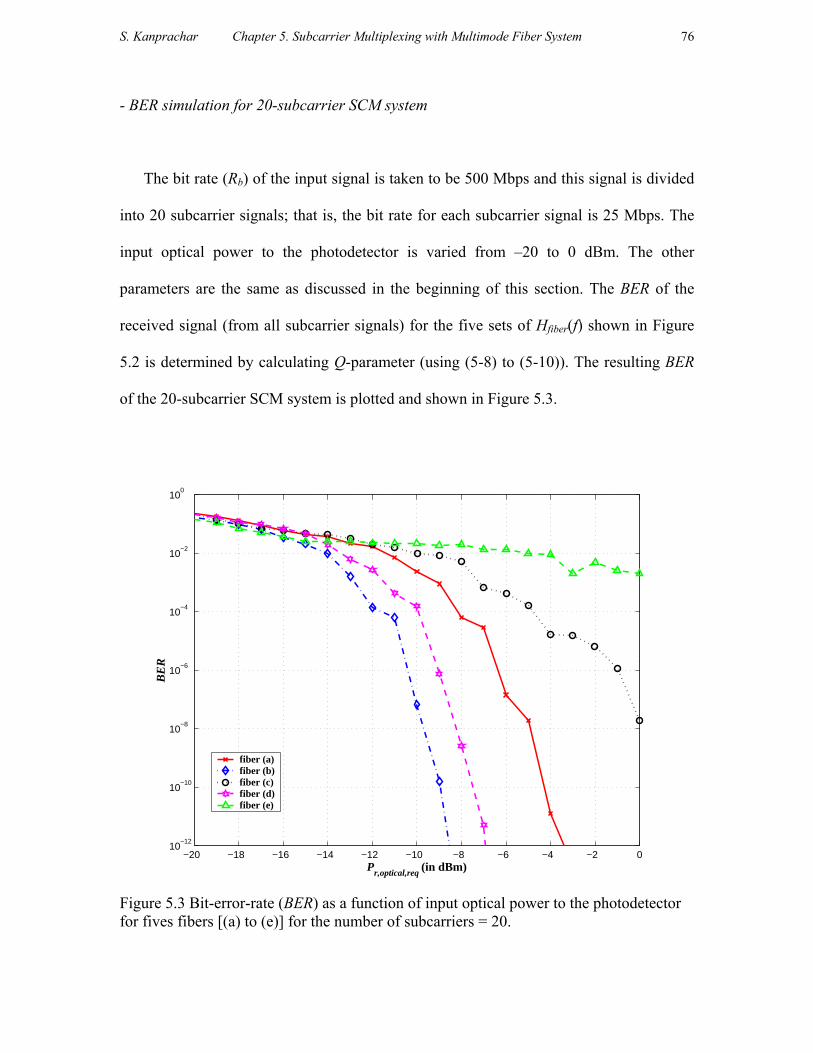
S. Kanprachar Chapter 5. Subcarrier Multiplexing with Multimode Fiber System
76
- BER simulation for 20-subcarrier SCM system
The bit rate (Rb) of the input signal is taken to be 500 Mbps and this signal is divided
into 20 subcarrier signals; that is, the bit rate for each subcarrier signal is 25 Mbps. The
input optical power to the photodetector is varied from –20 to 0 dBm. The other
parameters are the same as discussed in the beginning of this section. The BER of the
received signal (from all subcarrier signals) for the five sets of Hfiber(f) shown in Figure
5.2 is determined by calculating Q-parameter (using (5-8) to (5-10)). The resulting BER
of the 20-subcarrier SCM system is plotted and shown in Figure 5.3.
−20 −18 −16 −14 −12 −10 −8 −6 −4 −2 010
−12
10−10
10−8
10−6
10−4
10−2
100
Pr,optical,req (in dBm)
BE
R
fiber (a)fiber (b)fiber (c)fiber (d)fiber (e)
Figure 5.3 Bit-error-rate (BER) as a function of input optical power to the photodetector for fives fibers [(a) to (e)] for the number of subcarriers = 20.
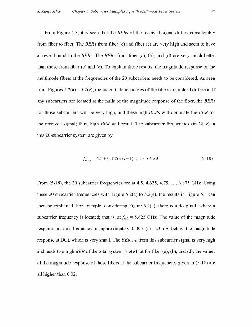
S. Kanprachar Chapter 5. Subcarrier Multiplexing with Multimode Fiber System
77
From Figure 5.3, it is seen that the BERs of the received signal differs considerably
from fiber to fiber. The BERs from fiber (c) and fiber (e) are very high and seem to have
a lower bound to the BER. The BERs from fiber (a), (b), and (d) are very much better
than those from fiber (c) and (e). To explain these results, the magnitude response of the
multimode fibers at the frequencies of the 20 subcarriers needs to be considered. As seen
from Figures 5.2(a) – 5.2(e), the magnitude responses of the fibers are indeed different. If
any subcarriers are located at the nulls of the magnitude response of the fiber, the BERs
for those subcarriers will be very high, and these high BERs will dominate the BER for
the received signal; thus, high BER will result. The subcarrier frequencies (in GHz) in
this 20-subcarrier system are given by
, 4.5 0.125 ( 1) ; 1 20sub if i i= + × − ≤ ≤ (5-18)
From (5-18), the 20 subcarrier frequencies are at 4.5, 4.625, 4.75, …, 6.875 GHz. Using
these 20 subcarrier frequencies with Figure 5.2(a) to 5.2(e), the results in Figure 5.3 can
then be explained. For example, considering Figure 5.2(e), there is a deep null where a
subcarrier frequency is located; that is, at fsub = 5.625 GHz. The value of the magnitude
response at this frequency is approximately 0.005 (or -23 dB below the magnitude
response at DC), which is very small. The BERSCM from this subcarrier signal is very high
and leads to a high BER of the total system. Note that for fiber (a), (b), and (d), the values
of the magnitude response of these fibers at the subcarrier frequencies given in (5-18) are
all higher than 0.02.

S. Kanprachar Chapter 5. Subcarrier Multiplexing with Multimode Fiber System
78
5.3 Effects of the number of subcarriers on bit-error-rate in SCM multimode fiber
system
It is shown in the previous section that the achieved BER of the SCM multimode fiber
system depends on the locations of the subcarrier frequencies relative to the deep nulls of
the magnitude response of the multimode fiber. However, the simulation done previously
is only for a 20-subcarrier system. It is interesting to study whether the BER can be
improved if the number of subcarriers is changed. In this section, the simulation similar
to the previous simulation is done for 10, 20, 30, 40, and 50 subcarriers for the same five
multimode fibers whose magnitude frequency response is shown in Figure 5.2. For all
cases, the total bandpass bandwidths in all cases are the same; that is, 3.25 GHz. As the
number of subcarriers increases, the bit rate per subcarrier (in Gbps) decreases and is
given by
,0.5
b subcarrier
RN
= (5-19)
And, the subcarrier frequencies (in GHz) for each case are defined by
,2.54.5 ( 1) ; 1sub i carriercarrier
f i i NN
= + × − ≤ ≤ (5-20)
The simulation results are presented in Figure 5.4. There are five curves in each
simulation plot corresponding to the five choices of Ncarrier, and there are five plots (a-e)
corresponding to the five fiber frequency responses from Figure 5.2.
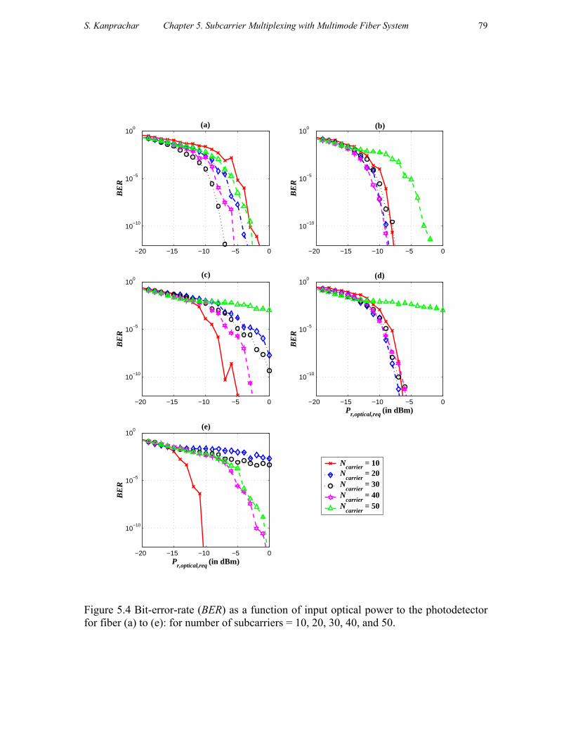
S. Kanprachar Chapter 5. Subcarrier Multiplexing with Multimode Fiber System
79
−20 −15 −10 −5 0
10−10
10−5
100 (a)
BE
R
−20 −15 −10 −5 0
10−10
10−5
100 (b)
BE
R
−20 −15 −10 −5 0
10−10
10−5
100
(c)
BE
R
−20 −15 −10 −5 0
10−10
10−5
100 (d)
Pr,optical,req (in dBm)
BE
R
−20 −15 −10 −5 0
10−10
10−5
100 (e)
Pr,optical,req (in dBm)
BE
R
Ncarrier = 10N
carrier = 20
Ncarrier
= 30N
carrier = 40
Ncarrier
= 50
Figure 5.4 Bit-error-rate (BER) as a function of input optical power to the photodetector for fiber (a) to (e): for number of subcarriers = 10, 20, 30, 40, and 50.
S. Kanprachar Chapter 5. Subcarrier Multiplexing with Multimode Fiber System
80
Considering the BER from different sets of Hfiber(f), it is seen that a good BER is
obtained for fibers (a) and (b); and, poor BER for fibers (c) and (e). These results are
consistent with the location of the nulls of the fiber frequency responses relative to the
subcarrier frequencies. Note that there are approximately 10 nulls in each of magnitude
responses shown in Figure 5.2, but the locations of these nulls are different.
Considering the number of subcarriers, it is seen from (5-19) that as Ncarrier is
increased, the individual subchannel bandwidths are decreased, which results in less
amplitude variation across a subchannel, and hence less intersymbol interference. This is
the big advantage of using subcarrier multiplexing with a wideband frequency-selective
channel. The BER of the system might then be expected to decrease as the number of
subcarriers increase. However, this is not totally true since there are other factors
affecting the achieved BER; that is, the relative locations of the subcarrier and null
frequencies. The larger the number of subcarriers, the larger is the possibility that some
of subcarriers are located at the nulls. For example, it is seen that from the simulation
results in Figure 5.4 Ncarrier = 50 never results in the best performance; indeed, in some
simulations, it is the poorest. This is the result of having many subcarriers located at the
nulls of the magnitude responses of the multimode fiber. To get small BER, the
subcarriers should not be located near any nulls of the fiber frequency response.
However, owing to changing environmental conditions this response may be time-
varying, and it cannot be guaranteed that the same set of subcarriers will be good for
sending the SCM signals all the time. Note that the probability of having k subcarriers
(from N-subcarrier system) located at the nulls will be analyzed in Chapter 8.

S. Kanprachar Chapter 5. Subcarrier Multiplexing with Multimode Fiber System
81
5.4 Conclusions
The bit-error-rate (BER) from the transmission system using subcarrier multiplexing
(SCM) on multimode fiber has been presented. The BER is determined using computer
simulation for 5 different sets of multimode fiber. The numbers of subcarriers used in the
simulation are 10, 20, 30, 40, and 50. It is shown that to get a good system performance
(i.e., low BER), the locations of subcarriers used in the system are very important. If there
are one or two subcarriers located at the deep nulls of the magnitude response, the BER
from those subcarrier signals will be very high. And, these high-BER subcarrier signals
will considerably degrade the total BER of the system; that is, a high BER results. The
effect of the number of subcarriers on the system performance has been shown. It is seen
that even though using a large number of subcarriers can reduce the amplitude variation
cause by the magnitude response of the multimode fiber since the bit rate per subcarrier
signal is small, the BER from the system with large number of subcarriers is not better
than the BER from the system with small number of subcarriers. Furthermore, in some
cases (for example, for Ncarrier = 50 in Figure 5.4(c)), the BER from the system with large
number of subcarrier is much higher than the BER from the system with small number of
subcarriers. The reason for this degradation, as noted previously, is the possibility of
having some subcarriers located at the deep nulls of the fiber response increases if the
number of subcarriers increases. The analysis of this probability will be given in Chapter
8. It is seen that even though the problem of having a wideband frequency-selective
channel is overcome by dividing the high bit rate signal into many small bit rate signals
and transmitting these signals via different subcarrier frequencies; the system

S. Kanprachar Chapter 5. Subcarrier Multiplexing with Multimode Fiber System
82
performance can still be degraded significantly if some subcarriers are at the deep nulls.
Therefore, to improve the system performance, some technique is needed to prevent or
cancel the effect of having some subcarriers located at deep nulls. In Chapters 6 and 7,
two techniques for doing this (that is, training process and diversity coding, respectively)
are studied.

S. Kanprachar Chapter 6. Training Process with Subcarrier Multiplexed Multimode Fiber System
83
Chapter 6
Training Process with Subcarrier Multiplexed
Multimode Fiber System
6.1 Introduction
The bit-error-rate (BER) of the received signal for the multimode fiber system using
subcarrier multiplexing (SCM) has been simulated, analyzed, and discussed in Chapter 5.
It was seen that the BER of the received signal depends mainly on the locations of the
subcarriers used in the system. If there are some subcarriers located at the deep nulls of
the magnitude response of the multimode fiber, the BER of the received signal is
degraded significantly; that is, BER is high. The effects of the number of subcarriers have
also been studied in Chapter 5. It was seen that using a large number of subcarriers does
not always give better system performance. The BER of the system with a large number
of subcarriers can be higher than the BER of the system with a small number of
subcarriers. This is explained by considering the likelihood of having subcarriers located
at the deep nulls which increases as the number of subcarriers increases. Hence, using a
smaller number of subcarriers is suggested. However, as the number of subcarriers is

S. Kanprachar Chapter 6. Training Process with Subcarrier Multiplexed Multimode Fiber System
84
reduced the achievable bit rate becomes smaller since the the bit rate per subcarrier signal
(Rb,SCM) should not be larger than one-half of the intermodal fiber bandwidth as shown in
Chapter 2.
The main problem with subcarrier multiplexing on multimode fiber is the deep nulls
in the frequency response of the fiber. To avoid the effect of having subcarriers located at
deep nulls, in this chapter, training sequences are used to determine the properties of all
subcarrier channels before transmitting the signal. All bad subcarrier channels are
dropped; and, only the good subcarriers channels are used in the signal transmission. It is
of interest to see how much this technique can improve the system performance relative
to that of the previous chapter. In the following sections, the BER of the received signal
from the subcarrier multiplexed multimode fiber system with training sequence is
presented. The effect on the BER of the number of channels dropped is studied.
6.2 Bit-error-rate of the received signal with 2 channels dropped
In this section, we consider the use of a training sequence to determine each channel’s
performance. This information is sent back to the transmitter so that only good channels
are used to transmit the data. Again, the same five multimode fibers, the magnitude
responses of which are shown in Figure 5.2, are used in the simulation. Only two values
(10 and 40) of the number of subcarriers are used in these simulations since these values
generally correspond to the best BERs in Chapter 5. Furthermore, it is assumed that

S. Kanprachar Chapter 6. Training Process with Subcarrier Multiplexed Multimode Fiber System
85
(Ncarrier + 2) training sequences are first sent through the system via different subcarriers
and the signal-to-noise ratios of these training signals are determined at the receiver. This
information is sent back to the transmitter, and the two poorest channels (in terms of
SNR) are dropped. Note that the effect of the number of channels dropped will be studied
in the next section. Then, only Ncarrier subcarriers are used for signal transmission. The
achieved BERs from the systems with and without training sequence for Ncarrier of 10 and
40 are shown in Figure 6.1. Other parameters are the same as used in Chapter 5. Note
that, for these 2 systems, the total bit rate is fixed at 500 Mbps. Therefore, the bit rates
per subcarrier are 50 and 12.5 Mbps, for the 10-subcarrier and 40-subcarrier systems,
respectively.
It is seen from Figure 6.1 that, as expected, the use of training improves performance.
For example, from Figure 6.1(a), at BER of 10-9, the required input optical power to the
photodetector for Ncarrier of 10 is decreased from -3 to -11 dBm, an 8 dB improvement.
Similarly, for Ncarrier of 40, the required input optical power to the photodetector is
decreased from -6 to -8.5 dBm, a 2.5 dB improvement. In general, it is seen that with the
use of training sequences the performance of the 10-subcarrier case is better than that of
the 40-subcarrier case. This can be explained by considering the number of subcarriers
possibly located at the deep nulls from these two subcarrier multiplexing systems and the
number of channels dropped out after the training. As discussed in Chapter 5, the number
of subcarriers located at the deep nulls for the 40-subcarrier case should be larger than
that for the 10-subcarrier case. In this section, for both cases, only the 2 poorest channels
are dropped after the training. For the 40-subcarrier case this number of channels dropped

S. Kanprachar Chapter 6. Training Process with Subcarrier Multiplexed Multimode Fiber System
86
may not be high enough to assure that no subcarriers will be located at the deep nulls. In
other words, the number of subcarriers located at the deep nulls from the 40-subcarrier
case may be larger than 2. Dropping only the 2 poorest channels still leaves some
subcarriers located at deep nulls, and these poor subcarrier channels can degrade the
performance of the system. However, as will be shown later in Section 6.3 for the 10-
subcarrier case it is highly unlikely that there are more than two subcarriers located at a
deep null.
It is seen in this section that the system performance is improved if the training is
used. The performance of the 10-subcarrier system is better than the performance of the
40-subcarrier system when 2 channels are dropped. Therefore with use of a training
sequence, it is unnecessary to use a large number of subcarriers. That is, for this study, a
10-subcarrier system with training sequence can offer good system performance.
However, in this section, only the 2 poorest channels are dropped after the training. It is
of interest to determine the system performance when the number of channels dropped is
varied. In the following section, the effect of the number of channels dropped on the 10-
subcarrier system is studied. The 10-subcarrier system is chosen since from this section
the performance of this system is better than the performance of the 40-subcarrier system;
thus, there is no need to consider a more complex system when we can get a better
performance from a system with less complexity.

S. Kanprachar Chapter 6. Training Process with Subcarrier Multiplexed Multimode Fiber System
87
−20 −15 −10 −5 0
10−10
10−5
100 (a)
BE
R
−20 −15 −10 −5 0
10−10
10−5
100
(b)
BE
R
−20 −15 −10 −5 0
10−10
10−5
100 (c)
BE
R
−20 −15 −10 −5 0
10−10
10−5
100 (d)
Pr,optical,req (in dBm)
BE
R
−20 −15 −10 −5 0
10−10
10−5
100 (e)
Pr,optical,req (in dBm)
BE
R
Ncarrier
= 10N
carrier = 10 with TS
Ncarrier
= 40N
carrier = 40 with TS
Figure 6.1 Bit-error-rate (BER) as a function of input optical power to the photodetector for fiber(a) to fiber(e): without and with training sequence (2 channels dropped), and number of subcarriers = 10 and 40.

S. Kanprachar Chapter 6. Training Process with Subcarrier Multiplexed Multimode Fiber System
88
6.3 Effects of the number of channels dropped on the achieved bit-error-rate: for
10-subcarrier system
From the results of the previous section it is seen that good system performance is
achieved with Ncarrier = 10 and with two channels dropped (i.e., initially doing
measurements on 12 channels.) Now we consider varying the number of channels that
are dropped. The frequency gap (∆fsub) between two consecutive subcarrier frequencies is
set to be five times the bit rate per subcarrier; that is, 5×50 = 250 MHz. During the
training process, (10 + Ndrop) training sequences are sent through the system via different
subcarriers to determine the SNR of each channel, and the Ndrop poorest channels (in
terms of SNR) are dropped out. In all cases 10 subcarrier frequencies are used for signal
transmission. The achieved BERs from the systems with Ndrop = 1, 2, 3 are shown in
Figure 6.2. Also, the achieved BER of the 10-subcarrier system without training is given
as a reference.
As expected, as Ndrop is increased performance is improved. The difference between
the required received optical power (Pr,optical,req) at BER of 10-9 from Ndrop of 1 and 2, and
from Ndrop of 2 and 3 is generally not significant; that is, approximately 1-dB difference
in most simulations. This may then suggest that using only 1 channel dropped is
sufficient. However, if there is more than 1 subcarrier located at the nulls, the difference
between the required received optical power (Pr,optical,req) at BER of 10-9 from Ndrop of 1
and 2 is quite large; approximately 5 dB as seen from the third simulation (Figure 6.2(c)),
but the additional improvement in going to Ndrop of 3 is insignificant; less than 0.5 dB.
This then suggests that for the 10-subcarrier SCM multimode fiber system in this study,
using training sequence with 2 channels dropped is the most suitable.

S. Kanprachar Chapter 6. Training Process with Subcarrier Multiplexed Multimode Fiber System
89
−20 −15 −10 −5 0
10−10
10−5
100
(a)
BE
R
−20 −15 −10 −5 0
10−10
10−5
100 (b)
BE
R
−20 −15 −10 −5 0
10−10
10−5
100 (c)
BE
R
−20 −15 −10 −5 0
10−10
10−5
100
Pr,optical,req
(in dBm)
(d)
BE
R
−20 −15 −10 −5 0
10−10
10−5
100
Pr,optical,req
(in dBm)
(e)
BE
R
No TSTS, dropping 1 channelsTS, dropping 2 channelsTS, dropping 3 channels
Figure 6.2: Bit-error-rate (BER) as a function of input optical power to the photodetector of 10-subcarrier SCM multimode fiber system for 5 different sets of multimode fiber: without and with training sequence (dropping 1, 2, and 3 channels).

S. Kanprachar Chapter 6. Training Process with Subcarrier Multiplexed Multimode Fiber System
90
6.4 Conclusions
The performance of subcarrier multiplexed multimode fiber system with training
process has been presented. The bit-error-rate (BER) has been determined for 10-
subcarrier and 40-subcarrier systems. It is seen that dropping only the 2 poorest channels
after the training can significantly improve the system performance in terms of BER,
especially for the 10-subcarrier system. And, the performance of the 10-subcarrier system
with training (dropping 2 channels) is better than the performance of the 40-subcarrier
system with training (dropping 2 channels). Hence, it is concluded that using a small
number of subcarriers system is preferred since it requires less system complexity and
gives better performance. Note that the number of subcarriers located at deep nulls for
different total number of subcarriers will be discussed in Chapter 8. The effect of number
of channels dropped after the training is also studied. It is shown that for the 10-
subcarrier system, 2 channels dropped after the training is the most suitable. Increasing
the number of channels dropped to 3, the additional improvement is insignificant.

S. Kanprachar Chapter 7. Diversity Coding with Subcarrier Multiplexed Multimode Fiber System
91
Chapter 7
Diversity Coding with Subcarrier Multiplexed
Multimode Fiber System
7.1 Introduction
Using training sequences with subcarrier multiplexed multimode fiber system, the
effect of having some subcarriers located at the deep nulls of the magnitude response of
the fiber is partially canceled since the properties of all subcarrier channels are
determined and only good channels are assigned to be the medium for signal
transmission.
Although the use of training sequences results in improved performance, it has
several disadvantages. The information at the receiver during the training process has to
be sent back to the transmitter for deciding which of the channels will be dropped. Also,
in the training process, Ncarrier+Ndrop subcarriers have to be used. This means that a
feedback circuit and extra subcarriers are needed. Also, the transmitter has to have the
ability to re-locate the data into the good subcarriers by using the information fed back

S. Kanprachar Chapter 7. Diversity Coding with Subcarrier Multiplexed Multimode Fiber System
92
from the receiver. There is also the further question of how rapidly the channels will
change, and consequently how frequently the training sequences will need to be sent.
To reduce this added complexity, instead of using training sequences, one may turn to
channel coding techniques; for example, convolutional codes and block codes [26- 30].
However, if coding is simply applied to each channel individually, the coding gain may
be insufficient for those channels located in a deep null of the frequency response. In this
chapter, we consider another technique called diversity coding, which is normally used in
network and data storage applications [31]. In this technique, some additional parity
subcarriers are added to the system. If there are any subcarriers located in deep nulls, the
data received from these subcarriers (called bad subcarriers) will be disregarded. The data
from these bad subcarriers will be recovered by the data received from good subcarriers.
This technique is very powerful since it can recover the lost data in bad subcarriers
almost instantaneously and there is no need to do the training process before
transmission.
In this chapter, the theory of diversity coding is first given [31]. The application of
diversity coding to the subcarrier multiplexed multimode fiber system is then studied.
Finally, the system performance in terms of bit-error-rate (BER) is analyzed and
simulated. It is shown that diversity coding results in performance comparable to that
achieved with training sequences, with however, considerably less complexity.
S. Kanprachar Chapter 7. Diversity Coding with Subcarrier Multiplexed Multimode Fiber System
93
7.2 Diversity coding theory [31]
The case in which there are N data channels and M parity channels is considered, and
the objective is to be able to recover the data in the presence of the loss of any M
channels. The input serial bits are divided into N data channels; thus, the data is sent in
parallel. In each symbol period (depending on the number of bits per symbol in the
diversity coding), the data symbols in all data channels are multiplied by the parity
generator matrix (P) to generate the parity symbols, which will be transmitted via parity
channels. The parity generator matrix P is given by
2 ( 1)
( 1)( 1) 2 4 2( 1)
( 1) 2( 1) ( 1)( 1)
1 1 1 11
[ ] [ ] 1
1
M
i j Mij N M N M
N N N M
Pα α α
β α α α α
α α α
−
− − −× ×
− − − −
= = =
(7-1)
The parity symbols (c) are given by
1 2 1 2[ , ,..., ] [ , ,..., ]M Nc c c c d d d P= = (7-2)
or 1
, 1 .N
j ij ii
c d j Mβ=
= ≤ ≤∑ (7-3)
where α is a primitive element in GF(2m)
cj is the data symbol in the jth parity channel; 1≤ j ≤ M
di is the data symbol in the ith data channel; 1≤ i ≤ N.
To recover any M failure channels from N+M channels, M parity channels are
required. The total number of channels transmitted is N+M channels. The number of bits
per data (and/or parity) symbol is given by 2log 1m N= + for M ≤ 3 (as will be
discussed later).

S. Kanprachar Chapter 7. Diversity Coding with Subcarrier Multiplexed Multimode Fiber System
94
At the receiver, assume that Nfailure channels from N+M channels are failure channels,
where 1≤ Nfailure ≤ M, and assume that n channels out of Nfailure failure channels are data
channels, and Nfailure-n out of Nfailure failure channels are parity channels. Since there are
Nfailure-n parity channels and Nfailure ≤ M, there are at least n good parity channels. To
recover n data failure channels, only n good parity channels are needed. Assume that,
1 2, , ,
nl l lc c c… where 1≤ l1 ≤ l2 ≤ …≤ ln ≤ M are available. The modified parity symbol jc
are generated by
1 2
1, , ,
; 1j j
n
N
j l il ii
i k k k
c c d j nβ=
≠
= + ≤ ≤∑…
(7-4)
Since [βij] or P are known at the transmitter and receiver, jc can be evaluated. To be able
to recover all lost data symbols (1 2, ,...,
nk k kd d d ) from 1 2, ,..., nc c c , the parameter jilβ has to
be chosen such that the following relationship can be inverted.
1 2, ,...,, 1 .
j
n
N
j il ii k k k
c d j nβ=
= ≤ ≤∑ (7-5)
It follows then that to recover1 2, ,...,
nk k kd d d , the matrix B, which is given by
1 1 1 2 1
2 1 2 2 2
1 2
n
n
j
n n n n
k l k l k l
k l k l k lil n n
k l k l k l
B
β β ββ β β
β
β β β×
= =
, (7-6)
has to have an inverse.

S. Kanprachar Chapter 7. Diversity Coding with Subcarrier Multiplexed Multimode Fiber System
95
Applying ( )( )1 1j
j
i lilβ α − −= to (7-6), we get that
11 1 1 2
22 1 2 2
1 2
( 1)( 1)( 1)( 1) ( 1)( 1)
( 1)( 1)( 1)( 1) ( 1)( 1)
( 1)( 1) ( 1)( 1) ( 1)( 1)
n
n
n n n n
k lk l k l
k lk l k l
k l k l k l
B
α α αα α α
α α α
− −− − − −
− −− − − −
− − − − − −
=
(7-7)
Even though α is a primitive element in GF(2m), it does not follow in general that B is
nonsingular and has an inverse. However, it has been shown in [31] that if the field
GF(2m) is chosen to be large enough, this matrix will be nonsingular. For M ≤ 3, the
minimum required m is given by 2log 1m N= + . If m satisfies this requirement, the
matrix B will have an inverse, and the failure data symbols 1 2, ,...,
nk k kd d d can be
recovered by
( ) ( )1 2
11 2, ,..., , ,...,
nk k k nd d d c c c B−= (7-8)

S. Kanprachar Chapter 7. Diversity Coding with Subcarrier Multiplexed Multimode Fiber System
96
7.3 Application of diversity coding to subcarrier multiplexed multimode fiber
system
Based on the results from Chapter 6, it is seen that good system performance can be
achieved from a 10-subcarrier system using a training sequence with 2 channels dropped.
Hence, in this chapter, diversity coding is applied to a 10-subcarrier SCM system with N
= 8 and M =2. To recover 2 failure channels, the parameter “m” has to be 4
(i.e., 2log 1m N= + , with N = 8). Thus, GF(24) is used in the coding process. A
primitive element, α, in GF(24) has to be used to construct the parity generator matrix, P.
To find a primitive element in GF(24), a 4th-degree primitive polynomial in GF(2) is
needed. Using this 4th-degree primitive polynomial to construct a table of cosets, the roots
of the 4th-degree primitive polynomial in GF(24) can be found. Since the roots of an mth-
degree primitive polynomial in GF(q)[x] are primitive elements in GF(qm), a primitive
element in GF(24) is also found.
From [32], a 4th-degree primitive polynomial in GF(2) is given by
4( ) 1p x x x= + + . Using this polynomial, a table for all possible cosets related to this
polynomial is shown below. Note that there are 16 elements in GF(24), and 15 of these
are non-zero elements.

S. Kanprachar Chapter 7. Diversity Coding with Subcarrier Multiplexed Multimode Fiber System
97
Table 7.1 All possible cosets related to 4( ) 1p x x x= + +
0×
p(x)
1×p(x) x×p(x) (x+1)
×p(x)
x2×
p(x)
(x2+1)
×p(x)
(x2+x)
×p(x)
…
0 0 x4+x+1 x5+x2+x x5+x4+
x2+1
x6+x3+
x2
x6+x4+
x3+x2+x+1
x6+x5+ x3+
x
…
1 1 x4+x x5+x2+x+
1
x5+x4+
x2
x6+x3+
x2+1
x6+x4+
x3+x2+x
x6+x5+ x3+
x+1
…
S x x4+1 x5+x2 x5+x4+
x2+x+1
x6+x3+
x2+x
x6+x4+
x3+x2+1
x6+x5+ x3 …
S+1 x+1 x4 x5+x2+1 x5+x4+
x2+x
x6+x3+
x2+x+1
x6+x4+
x3+x2
x6+x5+
x3+1
…
S2 x2 x4+x2+
x+1
x5+x x5+x4+1 x6+x3 x6+x4+ x3
+x+1
x6+x5+
x3+x2+x
…
S2+1 x2+1 x4+x2+
x
x5+x+1 x5+x4 x6+x3+
1
x6+x4+ x3
+x
x6+x5+
x3+x2+x+1
…
S2+S x2+x x4+x2+
1
x5 x5+x4+x+
1
x6+x3+
x
x6+x4+ x3+
1
x6+x5+ x3+
x2
…
S2+S
+1
x2+x
+1
x4+x2 x5+1 x5+x4+x x6+x3+
x+1
x6+x4+ x3 x6+x5+
x3+x2+1
…
S3 x3 x4+x3+
x+1
x5+x3+
x2+x
x5+x4+
x3+x2+1
x6+x2 x6+x4+
x2+x+1
x6+x5+x …
S3+1 x3+1 x4+x3+
x
x5+x3+
x2+x+1
x5+x4+
x3+x2
x6+x2+
1
x6+x4+ x2+x x6+x5+x+1 …
S3+S x3+x x4+x3+
1
x5+x3+
x2
x5+x4+
x3+x2+x+
1
x6+x2+
x+1
x6+x4+ x2+1 x6+x5 …
S3+S
+1
x3+x
+1
x4+x3 x5+x3+
x2+1
x5+x4+
x3+x2+x
x6+x2+
x+1
x6+x4+ x2 x6+x5+1 …
S3+S2 x3+
x2
x4+x3+
x2+x+1
x5+x3+x x5+x4+
x3+1
x6 x6+x4+ x+1 x6+x5+ x2+
x
…

S. Kanprachar Chapter 7. Diversity Coding with Subcarrier Multiplexed Multimode Fiber System
98
S3+S2
+1
x3+
x2+1
x4+x3+
x2+x
x5+x3+x+
1
x5+x4+
x3
x6 +1 x6+x4+x x6+x5+ x2+
x+1
…
S3+S2
+S
x3+
x2+x
x4+x3+
x2+ 1
x5+x3 x5+x4+
x3+x+1
x6+ x x6+x4+1 x6+x5+ x2 …
S3+S2
+S+1
x3+
x2+x
+1
x4+x3+
x2
x5+x3+1 x5+x4+
x3+x
x6+
x+1
x6+x4 x6+x5+
x2+1
…
Using Table 7.1, the roots of p(x) in GF(24) can be found as follows. There should be
4 roots for p(x) since the degree of p(x) is 4. Substituting all non-zero elements of GF(24)
into p(x), we obtain
For x=1, p(1) = 14 + 1 + 1 = 1. (≠ 0) (7-9)
For x=S, p(S) = S4 + S + 1 = (S+1) + S + 1 = 0. (7-10)
For x=S+1, p(S+1) = (S+1)4 + (S+1) + 1
= S4 +1 + (S+1) + 1
= (S+1) + 1 + (S+1) + 1 {from Table 7.1, S4 = S + 1}
= 0. (7-11)
For x=S2, p(S2) = (S2)4 + S2 + 1
= (S4)2 + S2 + 1
= (S+1)2 + S2 + 1 {from Table 7.1, S4 = S + 1}
= S2 + 1 + S2 + 1 = 0. (7-12)
For x=S2+1, p(S2+1)= (S2+1)4 + (S2+1) + 1
= (S4+1)2 + (S2+1) + 1
= ((S+1)+1)2 + (S2+1) + 1 {from Table 7.1, S4 = S + 1}
= S2 + (S2+1) + 1 = 0. (7-13)

S. Kanprachar Chapter 7. Diversity Coding with Subcarrier Multiplexed Multimode Fiber System
99
For x=S2+S, p(S2+S)= (S2+S)4 + (S2+S) + 1
= (S4+S2)2 + (S2+S) + 1
= ((S+1)+ S2)2 + (S2+S) + 1 {from Table 7.1, S4 = S + 1}
= (S4+S2 +1) + (S2+S) + 1
= ((S+1) + S2 +1) + (S2+S) + 1 = 1. (≠ 0) (7-14)
For x=S2+S+1, p(S2+S+1) = (S2+S+1)4 + (S2+S+1) + 1
= (S4+S2+1)2 + (S2+S+1) + 1
= (S2+S)2 + (S2+S+1) + 1 {from Table 7.1, S4 = S + 1}
= (S4+S2) + (S2+S+1) + 1
= ((S+1) + S2) + (S2+S+1) + 1 = 1. (≠ 0) (7-15)
For x=S3, p(S3) = (S3)4 + S3 + 1
= (S4)3 + S3 + 1
= (S+1)3 + S3 + 1 {from Table 7.1, S4 = S + 1}
= S3 + S2 + S + 1 + S3 + 1 = S2 + S. (≠ 0) (7-16)
For x=S3+1, p(S3+1)= (S3+1)4 + (S3+1) + 1
= (S6+1)2 + (S3+1) + 1
= ((S3+S2)+1)2 + (S3+1) + 1 {from Table 7.1, S6 = S3+ S2}
= (S6+S4+1) + (S3+1) + 1
= ((S3+S2) + (S+1)+1) + (S3+1) + 1
= S2 + S. (≠ 0) (7-17)

S. Kanprachar Chapter 7. Diversity Coding with Subcarrier Multiplexed Multimode Fiber System
100
For x=S3+S, p(S3+S)= (S3+S)4 + (S3+S) + 1
= (S6+S2)2 + (S3+S) + 1
= ((S3+S2)+ S2)2 + (S3+S) + 1 {from Table 7.1, S6 =S3+ S2}
= S6 + (S3+S) + 1
= (S3+S2)+ (S3+S) + 1
= S2+S+1. (≠ 0) (7-18)
For x=S3+S+1, p(S3+S+1) = (S3+S+1)4 + (S3+S+1) + 1
= (S6+S2+1)2 + (S3+S+1) + 1
= ((S3+S2) + S2 + 1)2 + (S3+S+1) + 1
= (S3+1)2 + (S3+S+1) + 1
= (S6+1) + (S3+S+1) + 1
= ((S3+S2) + 1) + (S3+S+1) + 1
= S2+S+1. (≠ 0) (7-19)
For x=S3+S2, p(S3+S2)= (S3+S2)4 + (S3+S2) + 1
= (S6+S4)2 + (S3+S2) + 1
= ((S3+S2) + (S+1))2 + (S3+S2) + 1
= (S6+S4+S2+1) + (S3+S2) + 1
= ((S3+S2) + (S+1) +S2+1) + (S3+S2) + 1
= S2+S+1. (≠ 0) (7-20)

S. Kanprachar Chapter 7. Diversity Coding with Subcarrier Multiplexed Multimode Fiber System
101
For x=S3+S2+1, p(S3+S2+1) = (S3+S2+1)4 + (S3+S2+1) + 1
= (S6+S4+1)2 + (S3+S2+1) + 1
= ((S3+S2) + (S+1) + 1)2 + (S3+S2+1) + 1
= (S3+S2+S)2 + (S3+S2+1) + 1
= (S6+S4+S2) + (S3+S2+1) + 1
= ((S3+S2) + (S+1) + S2) + (S3+S2+1) + 1
= S2+S+1. (≠ 0) (7-21)
For x=S3+S2+S, p(S3+S2+S) = (S3+S2+S)4 + (S3+S2+S) + 1
= (S6+S4+S2)2 + (S3+S2+S) + 1
= ((S3+S2) + (S+1) + S2)2 + (S3+S2+S) + 1
= (S3+S+1)2 + (S3+S2+S) + 1
= (S6+S2+1) + (S3+S2+S) + 1
= ((S3+S2) + S2 +1) + (S3+S2+S) + 1
= S2+S. (≠ 0) (7-22)
For x=S3+S2+S+1, p(S3+S2+S+1) = (S3+S2+S+1)4 + (S3+S2+S+1) + 1
= (S6+S4+S2+1)2 + (S3+S2+S)
= ((S3+S2) + (S+1) + S2 +1)2 + (S3+S2+S)
= (S3+S)2 + (S3+S2+S)
= (S6+S2) + (S3+S2+S)
= ((S3+S2) + S2) + (S3+S2+S)
= S2+S. (≠ 0) (7-23)

S. Kanprachar Chapter 7. Diversity Coding with Subcarrier Multiplexed Multimode Fiber System
102
From (7-9) to (7-23), it is seen that there are four roots of p(x) in GF(24); that is, S,
S+1, S2, and S2+1. Since the roots of an mth-degree primitive polynomial in GF(q)[x] are
primitive elements in GF(qm), then S, S+1, S2, and S2+1 are primitive elements in GF(24).
Let S be the chosen primitive element in GF(24); thus, α = S and α0, α1, α2, …,α14
will generate all non-zero elements in GF(24). Using this property with the table of all
cosets, the exponential, polynomial, and vector-space representations of GF(24) are
shown in Table 7.2.
Table 7.2 Exponential, polynomial, and vector-space representations of GF(24).
Exponential representation Polynomial representation Vector-space representation
0 0 [0 0 0 0]
α0 1 [1 0 0 0]
α1 α [0 1 0 0]
α2 α2 [0 0 1 0]
α3 α3 [0 0 0 1]
α4 1+α [1 1 0 0]
α5 α+α2 [0 1 1 0]
α6 α2+α3 [0 0 1 1]
α7 1+α+α3 [1 1 0 1]
α8 1+α2 [1 0 1 0]
α9 α+α3 [0 1 0 1]
α10 1+α+α2 [1 1 1 0]
α11 α+α2+α3 [0 1 1 1]
α12 1+α+α2+α3 [1 1 1 1]
α13 1+α2+α3 [1 0 1 1]
α14 1+α3 [1 0 0 1]

S. Kanprachar Chapter 7. Diversity Coding with Subcarrier Multiplexed Multimode Fiber System
103
From Table 7.2, it is seen that 4 input data bits in each data line (or subcarrier) can be
grouped to form a data symbol, which can be represented by the exponential format of
the primitive element α. Also, the parity generator matrix, P, and the parity symbols (i.e.,
c1 and c2) can then be constructed. The parity generator matrix, P, for this case (M = 2, N
= 8) is given by
1
2
7
1 111
1
Pαα
α
=
(7-24)
Using the above information, the data symbols from any two failure data channels can
be recovered at the receiver. To understand more clearly how the symbols from the
failure data channels can be recovered by using diversity coding, two examples are given
next. The first example is for the case that there is only one failure data channel and the
second example is for the case that there are two failure data channels in the system.
Example 1: one failure data channel.
The input serial bits to the SCM modulator are generated randomly and are given by
bit_in = [1 0 1 0 1 1 0 0
1 0 1 1 1 1 0 0
1 1 0 1 0 0 1 0
0 0 0 1 0 0 0 1] (7-25)
There are a total of 32 bits. These input bits are divided into 8 groups; thus, there are
4 bits in each group. The data bits in each group are sent to a particular data channel.

S. Kanprachar Chapter 7. Diversity Coding with Subcarrier Multiplexed Multimode Fiber System
104
Since there are 4 data bits in each data channel, these 4 bits can be represented by the
exponential representation as shown in Table 7.2; that is, we get
For data channel#1, bit_SCM= [ 1 1 1 0] d1 = α10
For data channel #2, bit_SCM= [ 0 0 1 0] d2 = α2
For data channel #3, bit_SCM= [ 1 1 0 0] d3 = α4
For data channel #4, bit_SCM= [ 0 1 1 1] d4 = α11
For data channel #5, bit_SCM= [ 1 1 0 0] d5 = α4
For data channel #6, bit_SCM= [ 1 1 0 0] d6 = α4
For data channel #7, bit_SCM= [ 0 0 1 0] d7 = α2
For data channel #8, bit_SCM= [ 0 0 0 1] d8 = α3
Thus, (d1, d2, d3, d4, d5, d6, d7, d8) = (α10, α2, α4, α11, α4, α4, α2, α3) (7-26)
Substituting (7-24) and (7-26) into (7-2), the parity symbols for the two parity channels,
channel#9 and channel#10, are given by
1 2 1 2 8
1
10 2 4 11 4 4 2 3 2
7
[ , ] [ , ,..., ]1 11
[ ] 1
1
c c c d d d P
αα α α α α α α α α
α
= =
=
= [α1, α10] (7-27)
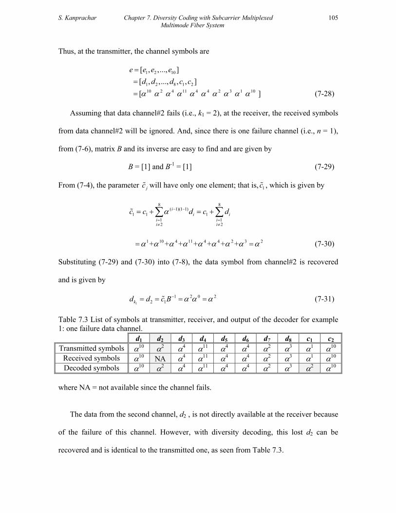
S. Kanprachar Chapter 7. Diversity Coding with Subcarrier Multiplexed Multimode Fiber System
105
Thus, at the transmitter, the channel symbols are
1 2 10
1 2 8 1 2
[ , ,..., ] [ , ,..., , , ]e e e e
d d d c c==
10 2 4 11 4 4 2 3 1 10 [ ]α α α α α α α α α α= (7-28)
Assuming that data channel#2 fails (i.e., k1 = 2), at the receiver, the received symbols
from data channel#2 will be ignored. And, since there is one failure channel (i.e., n = 1),
from (7-6), matrix B and its inverse are easy to find and are given by
B = [1] and B-1 = [1] (7-29)
From (7-4), the parameter jc will have only one element; that is, 1c , which is given by
8 8
( 1)(1 1)1 1 1
1 12 2
ii i
i ii i
c c d c dα − −
= =≠ ≠
= + = +∑ ∑
1 10 4 11 4 4 2 3 2 + + + + + + +α α α α α α α α α= = (7-30)
Substituting (7-29) and (7-30) into (7-8), the data symbol from channel#2 is recovered
and is given by
1
1 2 0 22 1kd d c B α α α−= = = = (7-31)
Table 7.3 List of symbols at transmitter, receiver, and output of the decoder for example 1: one failure data channel.
d1 d2 d3 d4 d5 d6 d7 d8 c1 c2 Transmitted symbols α10 α2 α4 α11 α4 α4 α2 α3 α1 α10
Received symbols α10 ΝΑ α4 α11 α4 α4 α2 α3 α1 α10 Decoded symbols α10 α2 α4 α11 α4 α4 α2 α3 α2 α10
where NA = not available since the channel fails.
The data from the second channel, d2 , is not directly available at the receiver because
of the failure of this channel. However, with diversity decoding, this lost d2 can be
recovered and is identical to the transmitted one, as seen from Table 7.3.

S. Kanprachar Chapter 7. Diversity Coding with Subcarrier Multiplexed Multimode Fiber System
106
Example 2: two failure data channels.
The input serial bits to the SCM modulator are again generated randomly and are now
given by
bit_in = [0 1 0 0 1 1 0 1
1 0 1 0 1 1 1 0
0 0 0 1 0 1 0 1
0 1 1 1 0 1 1 1] (7-32)
Similar to the first example, there are a total of 32 bits. As before, these input bits are
divided into 8 groups; thus, there are 4 bits in each group. The data bits in each group are
sent to a particular data channel. Since there are 4 data bits in each data channel, these 4
bits can be represented by the exponential representation as shown in Table 7.2; that is,
For data channel#1, bit_SCM= [0 1 0 0] d1 = α1
For data channel #2, bit_SCM= [1 0 0 1] d2 = α14
For data channel #3, bit_SCM= [0 1 0 1] d3 = α9
For data channel #4, bit_SCM= [0 0 1 1] d4 = α6
For data channel #5, bit_SCM= [1 1 0 0] d5 = α4
For data channel #6, bit_SCM= [1 1 1 1] d6 = α12
For data channel #7, bit_SCM= [0 1 0 1] d7 = α9
For data channel #8, bit_SCM= [1 0 1 1] d8 = α13
Thus, (d1, d2, d3, d4, d5, d6, d7, d8) = (α1, α14, α9, α6, α4, α12, α9, α13) (7-33)
S. Kanprachar Chapter 7. Diversity Coding with Subcarrier Multiplexed Multimode Fiber System
107
Substituting (7-24) and (7-33) into (7-2), the parity symbols for channel#9 and
channel#10 are now given by
1 2 1 2 8
1
1 14 9 6 4 12 9 13 2
7
[ , ] [ , ,..., ]1 11
[ ] 1
1
c c c d d d P
αα α α α α α α α α
α
= =
=
= [α5, α0] (7-34)
Thus, at the transmitter, the channel symbols are
1 2 10
1 2 8 1 2
[ , ,..., ] [ , ,..., , , ]e e e e
d d d c c==
= [α1 α14 α9 α6 α4 α12 α9 α13 α5 α0] (7-35)
Assuming that data channel#3 and channel #7 fail (i.e., k1 = 3 and k2 = 7), at the
receiver, the received symbols from these two data channels will be ignored. And, since
there are two failure channels (i.e., n = 2), from (7-6), matrix B is given by
1 1
2 2
( 1)(1 1) ( 1)(2 1) 2
2 2 ( 1)(1 1) ( 1)(2 1) 6
1[ ]
1
k k
ij k kBαα α
βαα α
− − − −
× − − − −
= = =
(7-36)
And, the inverse of matrix B is given by
6 2 6 2 6 2
16 2 32
6
1 1 11 1 1 1 1 11
det1
Bα α α α α α
α α ααα
− = = = −
3 14
12 12 α αα α
=
(7-37)

S. Kanprachar Chapter 7. Diversity Coding with Subcarrier Multiplexed Multimode Fiber System
108
From (7-4), the parameter jc will have two elements; that is, 1c and 2c , which are given
by
8 8
( 1)(1 1)1 1 1
1 13,7 3,7
ii i
i ii i
c c d c dα − −
= =≠ ≠
= + = +∑ ∑
5 1 14 6 4 12 13 + + + + + + 0α α α α α α α= = (7-38)
and 8 8
( 1)(2 1) ( 1)2 2 2
1 13,7 3,7
i ii i
i ii i
c c d c dα α− − −
= =≠ ≠
= + = +∑ ∑
0 1 0 9 8 2 5 12 + + + + + +α α α α α α α α= = (7-39)
Substituting (7-37) to (7-39) into (7-8), the data symbols from channel#3 and channel #7
are recovered and are given by
( ) ( ) ( )1 2
3 141 12 9 9
3 7 1 2 12 12, , , 0k kd d d d c c Bα α
α α αα α
− = = = =
(7-40)
Table 7.4 List of symbols at transmitter, receiver, and output of the decoder for example 2: two failure data channels.
d1 d2 d3 d4 d5 d6 d7 d8 c1 c2 Transmitted symbols α1 α14 α9 α6 α4 α12 α9 α13 α5 α0
Received symbols α1 α14 ΝΑ α6 α4 α12 ΝΑ α13 α5 α0 Decoded symbols α1 α14 α9 α6 α4 α12 α9 α13 0 α12
where NA = not available since the channel fails.
Now d3 and d7 at the receiver are ignored because of the line failures. However, with
diversity decoding, these lost d3 and d7 can be recovered and are identical to the
transmitted d3 and d7, as seen from Table 7.4.

S. Kanprachar Chapter 7. Diversity Coding with Subcarrier Multiplexed Multimode Fiber System
109
So far in this chapter the application of diversity coding to a 10-subcarrier SCM
multimode fiber system has been discussed. Some examples on how the data from the
failure data channels can be recovered using diversity coding have also been given.
Attention has been restricted to the case of 10 subcarriers, where 8 are for data channels
and 2 are for parity channels. It is seen from these examples that the data from failure
data channels can be recovered completely. Note that if the two failure channels are
parity channels, there is no need to do the decoding since all data from the data channels
are received correctly. Since the received data from the poorest and next poorest channels
are disregarded, it seems plausible that this is similar to the case of using training
sequences (with 12 subcarriers) and dropping the 2 poorest subcarriers. However, it is
necessary to verify that this is indeed the case. It should be noted that since 10 subcarriers
are needed during the actual transmission; for the system with training sequences, 12
subcarriers are used during the training and the 2 poorest subcarriers are dropped.
7.4 Analysis and simulation of bit-error-rate of subcarrier multiplexed multimode
fiber system with diversity coding
It is shown in the previous section that using diversity coding with a SCM multimode
fiber system, the data symbols from failure data channels can be recovered
instantaneously if the number of good parity channels is greater than or equal to the
number of failure data channels. There is no need of a training process to determine the

S. Kanprachar Chapter 7. Diversity Coding with Subcarrier Multiplexed Multimode Fiber System
110
channel’s properties; thus, the system is less complex. However, even though the data
from failure channels can be recovered, it does not mean that there is no error in the
recovered data. This error can happen since the lost data is recovered from the data from
good channels. But the word “good” does not mean that those data are completely error
free. The error from the data received from good channels will certainly affect the
recovered data; thus, increase the total bit-error-rate (BER) of the system. In the
remainder of this chapter a combined analysis and simulation of the BER is provided.
- BER analysis for the SCM multimode fiber system with diversity coding
Consider the general case of diversity coding in which there are N data channels, and
M parity channels, and the symbols consist of m bits. It is assumed that there are Nfailure
failure channels. Note that the maximum number of failure channels for which the data in
these failure channels can be recovered by using M for N diversity coding is M. Among
these Nfailure channels, assume as before that n channels are data channels and Nfailure – n
are parity channels. At the receiver, N+M-Nfailure channels are good channels and N
channels (N-n data channels and n parity channels) are used for the decoding process.
Note that if there are more than n good parity channels, the best n parity channels will be
used for decoding. Within these N channels, there certainly is a poorest channel, which is
taken to be the channel having the lowest signal-to-noise ratio (SNR). The recovered data
will be strongly affected by this poorest channel; that is, if the BER from this channel is
high, the probability that the recovered data will be wrong is also high; thus, the total
system BER will be high. It will be assumed that the BER from the worst subcarrier

S. Kanprachar Chapter 7. Diversity Coding with Subcarrier Multiplexed Multimode Fiber System
111
(among the N good channels) dominate the BER calculation of the recovered data. To
calculate the BER of the recovered data, the symbol-error-rate of this worst channel has
to be evaluated since now the data is represented in symbols (i.e., m bits per symbol).
Let BERSCM,worst be the BER of the worst channel (among N-n good data channels and
n good parity channels); that is,
{ }]
, , 1 2
1 2
min for 1 , , ,..., ;
for 1 , , ,...,
SCM worst SCM i n
n
BER BER SNR i N i k k k
N i N M i N l N l N l
= ≤ ≤ ≠+ ≤ ≤ + = + + +
(7-41)
where k1, k2,…, kn are the indices of the failure data channels, and
l1, l2,…, ln are the indices of the good parity channels.
To determine the probability of symbol error for this worst channel, the probabilities
of 1-bit error, 2-bit errors, …, m-bit errors in an m-bit symbol have to be determined. The
summation of these probabilities is the symbol-error-rate of the worst channel; that is,
, ,1Pr [ -bit error]
m
SCM worst SCM worstj
SER j=
= ∑ (7-42)
where PrSCM,worst[j-bit error] is the probability of j-bit error in m-bit symbol; 1 ≤ j ≤ m.
Assuming that the error bits are independent of one another, the probability of j-bit
error in m-bit symbol is given by
( ), , ,Pr [ -bit error]= 1m jj
SCM worst SCM worst SCM worst
mj BER BER
j−
−
(7-43)
Applying (7-43) to (7-42) the SER of the worst channel can be found. As assumed
previously the worst channel dominates the BER of the recovered data; thus, if the

S. Kanprachar Chapter 7. Diversity Coding with Subcarrier Multiplexed Multimode Fiber System
112
received symbol from the worst channel is wrong, the recovered symbol is also wrong.
That is, the SER of the recovered data is identical to the SER of the received data from the
worst channel and is given by
, cov ,
,1
Pr [ -bit error]
SCM re ered SCM worst
m
SCM worstj
SER SER
j=
=
= ∑
( ), ,1
1m m jj
SCM worst SCM worstj
mBER BER
j−
=
= −
∑ (7-44)
Note that the SER of the recovered data in (7-44) is an upper bound to SER since it is
determined from the SER of the received data from the worst channel.
From (7-42) to (7-44), with different values of BERSCM,worst, it is seen that if
BERSCM,worst, is very large (> 0.5), SERSCM,worst will also be very large (close to unity).
However, this is not an interesting region since we will not send the signal in this high
BER region. As BER SCM,worst becomes smaller, the probability of 1-bit error will become
large compared to the probabilities of 2-bit error, 3-bit error, and so on. Also, in this case,
the probability of 1-bit error is close to m×BERSCM,worst. Thus, with a small BERSCM,worst,
SERSCM,worst and SERSCM,recovered can be approximated by m×BERSCM,worst.
Using the SERSCM,recovered found previously, the bit-error-rate of the recovered data has
to be determined. Assuming that all possible recovered symbols (except the correct
symbol since now we are talking about the wrong symbol) are equally likely, then the
probability of each wrong recovered symbol is 12 1m −
since there are 2m–1 possible

S. Kanprachar Chapter 7. Diversity Coding with Subcarrier Multiplexed Multimode Fiber System
113
wrong symbols in GF(2m). Considering the vector-space presentation in GF(2m), for any
correct symbol, the number of possible wrong symbols that lead to i-bit error is given by
( )-bit error in -bit symbolm
K i mi
=
(7-45)
Using this information, it is found that
[ ], cov covPr -bit error in -bit symbol|2 1SCM re ered re ered correct m
mi
i m d d
≠ =
− (7-46)
where drecovered is the recovered symbol for the failure channel
dcorrect is the correct symbol for the failure channel.
And, the bit-error-rate of the recovered data (BERSCM,recovered) is given by
[ ], cov , cov cov1
Pr -bit error in -bit symbol|m
SCM re ered SCM re ered re ered correcti
BER SER i i m d d=
= × ≠∑
( ), ,1 1
12 1
m mm jjSCM worst SCM worst m
j i
mm i
BER BER ij
−
= =
= − × × −
∑ ∑ (7-47)
Note also that BERSCM,recovered in (7-47) is an upper bound BER since it is determined
from an upper bound SERSCM,recovered.
If BERSCM,worst is small (<10-2), the bit-error-rate of the recovered data (BERSCM,recovered)
can be approximated by

S. Kanprachar Chapter 7. Diversity Coding with Subcarrier Multiplexed Multimode Fiber System
114
, cov ,1 2 1
m
SCM re ered SCM worst mi
mi
BER m BER i=
≅ × × × −
∑ (7-48)
The BERs of all recovered carriers are assumed to be identical and given by (7-47). Note
that from (7-47) and (7-48), BERSCM,recovered will be larger than BERSCM,worst. Using (7-47)
and (7-48), the total BER of the system using M for N diversity coding with n failure data
channels is given by
1 2
, cov ,1
, ,...,
1
n
N
SCM re ered SCM ii
i k k k
BER n BER BERN =
≠
= × +
∑ (7-49)
where BERSCM,i is the bit-error-rate from ith-channel, which can be determined
from the Q-parameter (as defined in Chapter 5) corresponding to the ith-channel.
BERSCM,recovered is the bit-error-rate of the recovered channel, which can be
determined from (7-47).
From (7-49), it is seen that if all data channels are good (i.e., n = 0), there is no need
to do the decoding. Thus, in this case, BERSCM,recovered is not included in the calculation of
the total BER of the system.
Applying the results of this analysis to a 10-subcarrier system as discussed in the
previous section, the BER of that system can be determined. The number of total
subcarriers is 10; 8 of these are for data channels and 2 of these are for parity channels
(i.e., N = 8 and M = 2). 2 parity channels are for recovering 2 data failure channels. The
number of bits per symbol in each channel is 4; thus, m = 4. Since there are 2 parity

S. Kanprachar Chapter 7. Diversity Coding with Subcarrier Multiplexed Multimode Fiber System
115
channels, the maximum number of failure channels (Nfailure) is 2. Also, the maximum
number of failure data channels (n) is 2. That is, if n = 2, Nfailure is also 2 and all parity
channels (2 parity channels) must be good in order to recover two failure data channels.
Applying these parameters to the results of the BER analysis (i.e., (7-41) to (7-49)), the
total BER of the 10-subcarrier SCM system is given by
8
, cov ,1
;1
18
l
SCM re ered SCM ii
i k l n
BER n BER BER=
≠ ≤ ≤
= × +
∑ (7-50)
[ ]4
, cov , cov cov1
Pr -bit error|SCM re ered SCM re ered re ered correctj
BER SER j j d d=
= × ≠∑
, cov4 6 4 11 2 3 4
15 15 15 15SCM re eredSER = × × + × + × + ×
, cov3215 SCM re eredSER= (7-51)
( )4 4
, cov , ,1
41
jjSCM re ered SCM worst SCM worst
jSER BER BER
j−
=
= −
∑ (7-52)
{ }, ,min for 1 8, , 1 ;
for 9 10, 8 , 1
SCM worst SCM i j
j
BER BER SNR i i k j n
i i l j n
= ≤ ≤ ≠ ≤ ≤≤ ≤ = + ≤ ≤
(7-53)
where SNRSCM,i is the signal-to-noise ratio from the ith-channel
BERSCM,i is the bit-error-rate from the ith-channel, which can be determined from
the Q-parameter corresponding to ith-channel, which is obtained from system simulations
as discussed in the following section.

S. Kanprachar Chapter 7. Diversity Coding with Subcarrier Multiplexed Multimode Fiber System
116
- BER simulation for the SCM multimode fiber system with diversity coding
The block diagram of the SCM multimode fiber system with diversity coding is
shown Figure 7.1. The total number of subcarriers is N+M (N subcarriers for data
symbols and M subcarriers for parity symbols). The number of bits per symbol is m. The
input bit rate is Rb. Since there are N data carriers, the bit rate for each subcarrier will be
Rb,SCM = Rb/N. The data symbols from these N subcarriers are sent into the diversity
encoder to generate M parity symbols for M parity subcarriers. The parity symbols are
generated according to the procedure outlined in the previous section (Section 7.2). The
data from these N+M subcarriers is summed forming a bandpass electrical signal. This
signal is converted into an optical signal at the laser. This optical signal is then
transmitted through a multimode fiber. At the photodetector, the optical signal is detected
and converted back to an electrical signal. Thermal noise is added to this electrical signal.
The received electrical signal is sent to N+M different paths corresponding to N+M
different subcarriers. Each path contains a bandpass filter, a frequency-down converter
and a lowpass filter. The output signal of each path is the received signal for a particular
subcarrier. The signal-to-noise ratio (SNR) of the output signals of these N+M paths is
determined by simulation.
These SNRs are compared to one another. The signals of the M poorest subcarries (in
terms of SNRs) is disregarded; that is, Nfailure = M. If these M poorest subcarriers are
parity subcarriers, there is no need to do the decoding at the receiver, the received data
from all data subcarriers can be sent to the parallel-to-serial block immediately. And, the

S. Kanprachar Chapter 7. Diversity Coding with Subcarrier Multiplexed Multimode Fiber System
117
total BER of the system is just the average BER of the BERs of these data subcarriers,
which can be determined by their Q-parameters. However, if at least one of these M
poorest subcarriers is a data subcarrier, the signals from other good subcarriers (i.e., N
subcarriers) will be used in the diversity decoder to generate the signals for these M
poorest subcarriers.
The Q-parameter of each subcarrier signal can be determined by evaluating 4
parameters; that is, the averages and standard deviations of bits 0 and 1, as seen in (7-55).
These four parameters are determined at the receiver by simulation. Then, the BER
corresponding to each subcarrier signal can be determined using the Q-parameter; that is,
( )1 0, ,
1 0SCM i SCM iBER K K Qµ µ
σ σ −
= = + (7-54)
where QSCM,i is the Q-parameter corresponding to the ith-channel and is given by
1 0,
1 0SCM iQ µ µ
σ σ−
=+
(7-55)
( )2
212
u
xK x e du
π
−∞= ∫ (7-56)
µ1 = average value for bit 1
µ0 = average value for bit 0
σ1 = standard deviation for bit 1
σ0 = standard deviation for bit 0.

S. Kanprachar Chapter 7. Diversity Coding with Subcarrier Multiplexed Multimode Fiber System
118
BitGen S/P
Rb
Rb,SCM=RbN
f
0 dB|HFiber(f)|Multimode Fiberfsub,1
PulseGen
PulseGen
PulseGen
En-coder
fsub,2
fsub,N
PulseGen
PulseGen
fsub,N+1
fsub,N+M
Laser
N datalines
M paritylines
d1
d2
dN
c1
cM
Nthermal~ N(0,σth
2)
fGBP
BWBP
fsub,2
Bandpass filter
fGBP
BWBP
fsub,1
fGBP
BWBP
fsub,N+M
fsub,1
fsub,2
fsub,N+M
Lowpass filter
fGLP
BWLP
fGLP
BWLP
fGLP
BWLP
OFDMsignal
at fsub,1
OFDMsignalat fsub,2
OFDMsignal
at fsub,N+M
Rb,SCM=RbN
DecisionCircuit
DecisionCircuit
DecisionCircuitSquare-law
Detector2Atten-
uator(L)
d1
d2
cM
d1
d2
cM
dN
c1
FailureDetector P/S Received
Signal
Rb
d1
d2
dN
Decoder
N-n datalines
dk1
dkn
n recoveredlines
1cl
ncl
k1, k2, ..., kn and l1, l2, ..., ln
n parity lines
Figure 7.1 Diagram of subcarrier multiplexed multimode fiber system with diversity coding.
As indicated previously the simulation is conducted for a 10-subcarrier system in
which eight subcarriers are used for data symbols and two subcarriers are for parity
symbols. The total bit rate is 500 Mbps. Since there are 8 data subcarriers, the bit rate for
each subcarrier will be 500/8 = 62.5 Mbps. The number of bits per symbol is 4. Other

S. Kanprachar Chapter 7. Diversity Coding with Subcarrier Multiplexed Multimode Fiber System
119
parameters are the same as used in Chapter 5. The SNR of the output signals of the 10
subcarriers is determined, and the two poorest are discarded; that is, Nfailure = 2. If these
two poorest subcarriers are parity subcarriers, there is no need to do the decoding at the
receiver, and the total BER of the system is just the average BER of these data
subcarriers, which can be determined by their Q-parameters. However, if at least one of
these two poorest subcarriers is a data subcarrier, the signals from the other good
subcarriers are used in the diversity decoder to generate the signals for these two poorest
subcarriers. Using the information from the simulation, the Q-parameters of these 8 good
subcarriers can be determined; thus, the BERs for all 8 good subcarriers can be evaluated.
The worst BER among these 8 BERs will be used as BERSCM,worst (see (7-53)). With this
BERSCM,worst and the result from the analysis from the previous section, the total BER of
the system can then be determined.
The BER simulations for different sets of multimode fiber and different system
modifications are given in Figures 7.2 and 7.3. There are five plots in Figure 7.2
corresponding to the five different sets of multimode fiber as shown in Figure 5.2. In
each of these five plots, there are three BER curves corresponding to the following three
cases: (1) no training and no diversity coding, (2) training with dropping 2 channels, and
(3) diversity coding with 2 parity channels

S. Kanprachar Chapter 7. Diversity Coding with Subcarrier Multiplexed Multimode Fiber System
120
−20 −15 −10 −5 0
10−10
10−5
100 (a)
BE
R
−20 −15 −10 −5 0
10−10
10−5
100 (b)
BE
R
−20 −15 −10 −5 0
10−10
10−5
100 (c)
BE
R
−20 −15 −10 −5 0
10−10
10−5
100
Pr,optical,req (in dBm)
(d)
BE
R
−20 −15 −10 −5 0
10−10
10−5
100
Pr,optical,req (in dBm)
(e)
BE
R
No TS, No DCTS, dropping 2 channelsDC, 2 parity channels
Figure 7.2 Comparison of performance of (1) no training sequence or diversity coding (No TS, No DC), (2) training sequence with two dropped channels, and (3) diversity coding with 2 parity channels. The five plots (a)-(e) correspond to the five different sets of multimode fiber from Figure 5.2
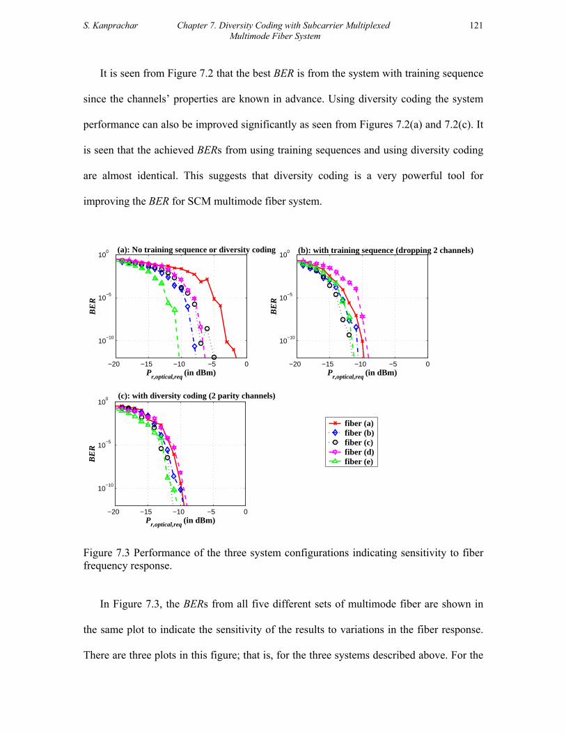
S. Kanprachar Chapter 7. Diversity Coding with Subcarrier Multiplexed Multimode Fiber System
121
It is seen from Figure 7.2 that the best BER is from the system with training sequence
since the channels’ properties are known in advance. Using diversity coding the system
performance can also be improved significantly as seen from Figures 7.2(a) and 7.2(c). It
is seen that the achieved BERs from using training sequences and using diversity coding
are almost identical. This suggests that diversity coding is a very powerful tool for
improving the BER for SCM multimode fiber system.
−20 −15 −10 −5 0
10−10
10−5
100 (a): No training sequence or diversity coding
Pr,optical,req (in dBm)
BE
R
−20 −15 −10 −5 0
10−10
10−5
100 (b): with training sequence (dropping 2 channels)
Pr,optical,req (in dBm)
BE
R
−20 −15 −10 −5 0
10−10
10−5
100 (c): with diversity coding (2 parity channels)
Pr,optical,req (in dBm)
BE
R
fiber (a)fiber (b)fiber (c)fiber (d)fiber (e)
Figure 7.3 Performance of the three system configurations indicating sensitivity to fiber frequency response.
In Figure 7.3, the BERs from all five different sets of multimode fiber are shown in
the same plot to indicate the sensitivity of the results to variations in the fiber response.
There are three plots in this figure; that is, for the three systems described above. For the

S. Kanprachar Chapter 7. Diversity Coding with Subcarrier Multiplexed Multimode Fiber System
122
case of no training sequence or diversity coding (Figure 7.3(a)), the variation of
Pr,optical,req is approximately 8 dB at BER of 10-9. From Figures 7.3(b) and 7.3(c) this
variation is only 2.5 dB when either training sequences or diversity coding is used. Note
also that the training sequence and diversity coding cases have essentially the same
average Pr,optical,req (-11 dBm at BER of 10-9 ).
7.5 Conclusions
The theory of diversity coding, which is normally used in network and data storage
applications, is given. In diversity coding, at the transmitter, the symbols from all data
channels are used to generate the parity symbols, which are transmitted via parity
channels. At the receiver, if there are some failure channels, the received data from those
failure channels are discarded. The data from those failure channels can be recovered by
the received data from all other good channels. The application of this diversity coding to
the SCM multimode fiber system in order to cancel the effects of having some subcarriers
located at the deep nulls of multimode fiber has been studied. The BER analysis for the
SCM multimode fiber system with diversity coding is given. The results from the BER
simulation for a 10-subcarrier SCM multimode fiber system with diversity coding (2
parity channels) are presented. It is seen that the performance of the system with diversity
coding is much better than the performance of the system without coding or training.
Comparing the performance between the system with a training sequence (2 channels
dropped) and the system with diversity coding (2 parity channels), the performance of

S. Kanprachar Chapter 7. Diversity Coding with Subcarrier Multiplexed Multimode Fiber System
123
these two systems is almost identical. However, with diversity coding, a training is not
required; thus, there is less system complexity. Moreover, if the frequency response of
the multimode fiber is slowly time-varying, the system with a training process is required
to send the training sequence to update the channel property more frequently. In the
system with diversity coding, there is no need to update the channel property since the
data from the failure data channels can be recovered at the receiver. This then suggests
that diversity coding is a very powerful technique for canceling the effects of having
some subcarriers located at the deep nulls of the multimode fiber magnitude response.

S. Kanprachar Chapter 8. Practical Performance Limits and System Capacity
124
Chapter 8
Practical Performance Limits and System Capacity
8.1 Introduction
The performance of the subcarrier multiplexed multimode fiber system with different
system modifications has been presented in Chapters 5-7. In the examples considered the
bit rate of the transmitted signal is 500 Mbps, which is five times larger than the
intermodal bandwidth supported by the multimode fiber. The achieved BER at this bit
rate depends on many factors; that is, the bandwidth of each subcarrier, the number of
subcarriers, and the locations of the subcarriers in the frequency domain relative to the
nulls in the frequency response of the multimode fiber. From the results given in Chapter
5, it is seen that using a larger number of subcarriers does not always give a small BER.
On the other hand, if the number of subcarriers is small, the bandwidth of each subcarrier
needs to be large to achieve the given bit rate. These larger bandwidth subcarriers will
then be significantly affected by the amplitude variation of the frequency response of the
multimode fiber. Thus, the resulting BER from a small number of subcarriers can become
large, as well. The above considerations apply to the case of a fixed total bit rate. Also,
since the results are for a fixed fiber bandwidth, they apply for a fixed transmission

S. Kanprachar Chapter 8. Practical Performance Limits and System Capacity
125
distance. In this chapter we consider the factors affecting the total bit rate, transmission
distance and BER of a subcarrier multiplexed (SCM) system in multimode fibers.
Assuming that no modifications are made to the system (that is, no training process
and no diversity coding), there are two main factors affecting the total BER of the SCM
multimode fiber system; that is, the total bandpass bandwidth and the number of
subcarriers.
1) The total bandpass bandwidth of the fiber
In the model considered in Chapter 2, the results appear to indicate that there is no
limit to the bandpass bandwidth of the multimode fiber. However, in Chapter 2, only the
effect of modal dispersion was considered. If the transmission bandwidth becomes very
large, another type of dispersion, called chromatic dispersion should be taken into
account, as well. By considering the effect of chromatic dispersion, the upper limit of the
bandpass bandwidth of multimode fiber can be determined. It is of interest to determine
how large the bandpass bandwidth of the multimode fiber can be if the chromatic
dispersion is considered.
2) The number of subcarriers (Ncarrier) of the SCM multimode fiber system.
From the analysis in Chapter 2, it is seen that the available bandwidth for one
frequency band in the high frequency region is comparable to the intermodal bandwidth
(BWintermodal) of the multimode fiber. This means that if all subcarriers in the SCM
multimode fiber system are located at the middle of each passband region, the bandwidth
of each subcarrier signal should be less than the intermodal bandwidth so that the major

S. Kanprachar Chapter 8. Practical Performance Limits and System Capacity
126
portion of frequency response of all subcarrier signals will not be located at the nulls of
the fiber frequency response. This will increase the signal power and signal quality at the
receiving end, and certainly decrease the system BER. Since both side-bands of each
subcarrier signal are included in the transmission, the maximum bit rate of each
subcarrier signal should be less than one-half of the intermodal bandwidth. From this
point of view, it is seen that if the total bit rate is fixed, the number of subcarriers should
be large enough to make the bit rate of each subcarrier signal less than one-half of the
intermodal bandwidth.
However, as the number of subcarriers increases, it is shown in Chapter 5 that the
system performance is not always improved since the effect of deep nulls in the bandpass
region of the fiber becomes a major degradation to the system. The possibility that some
of subcarriers are located at the deep nulls becomes larger as the number of subcarriers
increases. This means that there will be more subcarriers located at the deep nulls. Hence,
the performance of the system with a large number of subcarriers can be degraded
significantly.
From this discussion, it is seen that the number of subcarriers is an important
parameter. For a fixed total bit rate, if the number of subcarriers is too small, the
bandwidth of each subcarrier signal may be larger than one-half of the intermodal
bandwidth of the fiber; thus, the amplitude variation within the bandpass region can
degrade the system performance. On the other hand, if the number of subcarriers is large,
there will be more subcarriers located at the deep nulls; thus, the achieved bit-error-rate
S. Kanprachar Chapter 8. Practical Performance Limits and System Capacity
127
(BER) becomes high. The available bandwidth of each possible passband region has been
analyzed in Chapter 2. Hence, the lower limit of the number of subcarriers can be
determined by using the intermodal bandwidth of multimode fiber if the total
transmission bit rate is fixed. However, the number of subcarriers located at the nulls of
the fiber in the high frequency range has not been considered. It is important then to
determine the number of subcarriers located at the nulls as a function of the number of
subcarriers used in the SCM system.
In the following sections, the effect of chromatic dispersion on the bandpass
bandwidth of multimode fiber is discussed. The number of subcarriers located at the nulls
of multimode fiber at high frequencies is then analyzed. Finally, the bit rate and distance
limitations of the SCM multimode fiber system are presented.
8.2 Effect of chromatic dispersion on the available bandpass bandwidth of
multimode fiber
It appears from the analysis in Chapter 2 that the bandpass bandwidth of the
multimode fiber is unlimited. However, in multimode fibers, another type of dispersion,
namely chromatic dispersion, becomes a limiting factor at high frequency. In this section,
the effect of chromatic dispersion on the bandpass bandwidth of multimode fibers is
discussed.

S. Kanprachar Chapter 8. Practical Performance Limits and System Capacity
128
Chromatic dispersion can be divided into two types; that is, waveguide dispersion and
material dispersion. Waveguide dispersion is very important in singlemode fibers since
the optical signal launched into the fiber travels to the end of the fiber via core and
cladding. The major portion of the signal travels within the core, and the rest within the
cladding. Because of the difference between the refractive indexes in the core and
cladding, the optical signal travels through the core and cladding with different velocities,
resulting in the pulse spreading at the receiving end. This type of chromatic dispersion is
negligible in multimode fiber transmission since the size of the core in multimode fibers
is very large; thus, most of the optical signal is confined in the core. On the other hand,
material dispersion, which is caused by the wavelength dependence of the refractive
index of the fiber core, can become a limiting factor in the multimode fiber transmission
if the operating wavelength is far from the zero-dispersion wavelength and/or the spectral
width of the optical source is large. The pulse spreading per unit length caused by
material dispersion is given by
( )material materialDτ λ λ∆ = × ∆ (8-1)
where Dmaterial(λ) is the material dispersion parameter depending on operating
wavelength, λ.
∆λ is the spectral width of the optical source.
From (8-1), the approximate bandwidth-distance product due to material dispersion is
given by [39]

S. Kanprachar Chapter 8. Practical Performance Limits and System Capacity
129
14material
material
BLτ
=∆
(8-2)
To consider the material dispersion parameter, the operating wavelength, λ, has to be
considered. There are three important operating wavelength regions in fiber optic
transmission; that is, at 850, 1300, and 1550 nm. The 850-nm operating wavelength was
the first wavelength used in practical fiber optic transmission in the 1970s. Even though
this wavelength does not offer either the lowest material dispersion or fiber attenuation,
in the 1970s, good sources and detectors were only available at this wavelength. The next
operating wavelength is located at 1300 nm. At this wavelength, the fiber attenuation is
very small compared to the fiber attenuation at the wavelength of 850 nm. However, the
most attractive property of the wavelength at 1300 nm is that at this wavelength, the
material dispersion is very small, close to zero-dispersion for silica based fibers. For the
wavelength of 1550 nm, the material dispersion is larger than the material dispersion at
1300 nm. However, what makes this wavelength interesting is that the fiber attenuation at
1550 nm is even lower; it can be as low as 0.2 dB/km [1]. So from this discussion, it is
seen that the smallest material dispersion is achieved at the 1300-nm operation
wavelength. However, it is of interest to consider some numerical examples of this
material dispersion parameter so that we can compare the bandwidth-distance product
limited by the material dispersion.

S. Kanprachar Chapter 8. Practical Performance Limits and System Capacity
130
Using the three-term Sellmeier equation, the material dispersion parameter is
approximated by [1]
( )4
0 014materialSD λ λλ
λ = −
(8-3)
where S0 is the zero-dispersion slope and λ0 is the zero-dispersion wavelength.
From [40], for 50/125 graded-index multimode fibers, λ0 is 1305 nm and S0 is 0.096
ps/(nm2⋅km). Applying these parameters to (8-3) for different operating wavelengths, we
get that
- for λ = 850 nm, Dmaterial(λ) = −92.94 ps/(nm⋅km) (8-4)
- for λ = 1300 nm, Dmaterial(λ) = −0.48 ps/(nm⋅km) (8-5)
- for λ = 1550 nm, Dmaterial(λ) = 18.50 ps/(nm⋅km) (8-6)
From (8-4) to (8-6), it is seen that the smallest material dispersion parameter is from
the operating wavelength of 1300 nm. However, to determine the bandwidth-distance
product due to the material dispersion, the spectral width of the optical source has to be
considered. Because of the low power coupled into a fiber, the small modulation
bandwidth, and very large spectral width offered by LEDs, LEDs are not suitable for high
bit-rate transmission using subcarrier multiplexing on multimode fibers. An alternative
choice is vertical cavity surface-emitting lasers (VCSELs), which have been used in
many research experiments for data transmission using subcarrier multiplexing on
multimode fibers. Thus, in this discussion, it is assumed that the VCSEL is used as the

S. Kanprachar Chapter 8. Practical Performance Limits and System Capacity
131
optical source in the transmitter. The spectral width of a VCSEL is very small. A spectral
width of 0.5 nm is available in commercial devices [40]. Assuming ∆λ = 0.5 nm; using
(8-1), (8-2) and (8-4) to (8-6), the bandwidth-distance products due to the material
dispersion for different operating wavelengths are given as follows
- for λ = 850 nm, BLmaterial(λ) = 2.7 GHz⋅km (8-7)
- for λ = 1300 nm, BLmaterial(λ) = 517.8 GHz⋅km (8-8)
- for λ = 1550 nm, BLmaterial(λ) = 13.5 GHz⋅km (8-9)
From (8-7) to (8-9), it is seen that if the data is transmitted within the intermodal
bandwidth of the multimode fiber, the effect of material dispersion can be neglected since
the bandwidth-distance product (approximately 400 MHz⋅km) of the intermodal
bandwidth from modal dispersion is much less than the bandwidth-distance product due
to the material dispersion. However, in data transmission using the passband region of the
multimode fiber, the effect of material dispersion can become a limiting factor if the
subcarrier frequencies are larger than the material dispersion bandwidth. This can also be
explained graphically by using Figure 8.1.

S. Kanprachar Chapter 8. Practical Performance Limits and System Capacity
132
|HFiber(f)|
f
0 dB
from modal dispersionfrom material dispersion
f1fintermodal f3-dB,mat
Figure 8.1 Illustration of frequency response of multimode fiber due to modal and material dispersion.
An illustration of the frequency response of the multimode fiber resulting from modal
dispersion and material dispersion is shown in Figure 8.1. It is seen that if the
transmission bandwidth is very small; that is, within the intermodal bandwidth, the effect
of material dispersion is negligible. For transmission using subcarrier multiplexing on
multimode fibers, the bandpass region of multimode fibers has to be used. If the modal
dispersion is the only dispersion taken into account, it is seen that the available bandpass
bandwidth is unlimited. However, this is not true since at this high frequency region, the
effect of material dispersion is significant and limits the available bandpass bandwidth to
be less than the frequency f1, as shown in Figure 8.1.
Applying the effect of material dispersion to the transmission bandwidth used in the
simulations of subcarrier multiplexing on multimode fibers in Chapter 5 to 7, it is seen
that since the maximum transmission frequency is approximately 8 GHz, the operating
wavelengths suitable for this transmission are at 1300 nm and 1550 nm. However, to

S. Kanprachar Chapter 8. Practical Performance Limits and System Capacity
133
guarantee that there will be no limitation on the bandpass bandwidth (at least up to 500
GHz), the operating wavelength at 1300 nm is chosen.
From the discussion in this section, it is seen that the material dispersion is very
important for bandpass transmission using multimode fibers. This dispersion can limit the
available bandpass bandwidth, which seems to be unlimited if only modal dispersion is
considered. The maximum bandpass bandwidth due to material dispersion depends on
two parameters; that is, the operating wavelength and the spectral width of the optical
source. The appropriate operating wavelength is at 1300 nm since at this wavelength the
material dispersion parameter is nearly minimized. For subcarrier multiplexing on
multimode fibers, a vertical cavity surface-emitting laser (VCSEL) is used as an optical
source in the transmitter. The spectral width of a VCSEL is very small; that is,
approximately 0.5 nm can be achieved. Using the 1300-nm operating wavelength with a
VCSEL with a spectral width of 0.5 nm, the maximum bandpass bandwidth-distance
product can be up to 500 GHz⋅km, which is very large compared to the transmission
bandwidth required by the simulations in Chapter 5 to 7. Operating at a wavelength of
1300 nm, the maximum bandwidth will be limited by practical microwave circuit
considerations rather than by material dispersion.
S. Kanprachar Chapter 8. Practical Performance Limits and System Capacity
134
8.3 Number of subcarriers located at deep nulls
8.3.1 Probability of having k subcarriers (from an N-subcarrier system) located at the nulls
From the simulation results in Chapter 5, it is seen that using a large number of
subcarriers does not guarantee that the achieved bit-error-rate (BER) will always be low,
though the bit rate per subcarrier is low. On the other hand, the achieved BER of the
system using a small number of high bit rate subcarriers is generally not high. Moreover,
in some cases, the BER from the system with a small number of subcarriers is lower than
that from the system with a large number of subcarriers. The reason for this, as discussed
qualitatively in Chapter 5, is mainly from the locations of the subcarriers relative to the
nulls in the transmission bandwidth. If there are many subcarriers located at the nulls of
the magnitude response of the multimode fiber, the BER for those subcarrier signals will
then be high; thus, resulting in a high system BER. The possibility of having some
subcarriers located at the nulls depends on the number of subcarriers in the system. In this
section, the probability of having k subcarriers (from an N-subcarrier system) located at
the nulls of multimode fibers is studied. The results from the analysis in Chapter 2 are
used.
Assumptions:
- The maximum subcarrier frequency is less than the passband bandwidth limited by
chromatic dispersion. The passband bandwidth limited by chromatic dispersion is very
large. If the operating wavelength is at 1300 nm, the maximum bandwidth-distance
product is 500 GHz ⋅km. It is assumed that 10% of this bandwidth-distance product is

S. Kanprachar Chapter 8. Practical Performance Limits and System Capacity
135
used; that is, the maximum bandwidth-distance product limited by chromatic dispersion
is 50 GHz ⋅km.
- The frequency spacing between two adjacent subcarriers is greater than the intermodal
bandwidth of the multimode fiber. With this assumption, the amplitudes of the magnitude
response of the multimode fiber from two subcarriers are essentially independent of one
another. This was shown in Chapter 2 by the correlation function of the frequency
response of the multimode fiber in the high frequency region. This correlation function is
approximately zero if the separation between two subcarriers is greater than the
intermodal bandwidth.
- The amplitude (Anull) of a null is defined by a ratio (ε) compared to the average
amplitude ( ( )fiberH fm ) of the magnitude response of the multimode fiber; that is,
( )fibernull H fA mε= (8-10)
Note: ε should be much smaller than unity for the signal to be considered to be at a null.
The amplitude of the null is said to be 1010log ε dB below the average amplitude.
From the above assumptions, the probability of having k subcarriers (from an N-
subcarrier system) located at nulls (with at least 1010log ε dB below the average
amplitude) has a Binomial distribution and is given by

S. Kanprachar Chapter 8. Practical Performance Limits and System Capacity
136
( ) ( )( ) ( )( ), , 1fiber fiber
N kk
H f H f
NP k N F m F m
kε ε ε
− = ⋅ − (8-11)
where ( )
!! !
N Nk k N k
= −
( )( )fiberH fF mε is the probability that the amplitude of the frequency response in
the passband region is less than Anull (or ( )fiberH fmε ).
It is seen that to determine the probability in (8-11), ( )( )fiberH fF mε has to be
determined. It is found from Chapter 2 that the magnitude response of multimode fibers
at high frequencies is Rayleigh distributed. Letting ( )fiberX H f= , the probability density
function (fX(x)) of X and its expected value (mX) are given by
( ) ( )2
222
x
Xxf x e U xσ
σ
−= (8-12)
( ) 2fiberX H fm m π σ= = (8-13)
where U(x) is the unit-step function.
From (8-12), the probability that the amplitude of the frequency response of
multimode fibers in the passband region is less than x is given by
( ) ( )2 2
2 22 22
0 0
1u xx x
XuF x f u du e du eσ σ
σ
− −
= = = −∫ ∫ (8-14)
S. Kanprachar Chapter 8. Practical Performance Limits and System Capacity
137
Substituting ( )fiberH fmε for x into (8-14), we get
( )( ) ( )2 2
221X
fiber
m
XH fF m F m eε
σε ε−
= = − (8-15)
Substituting mX from (8-13) into (8-15), we get
( )( ) ( )2
41fiber
XH fF m F m eπ ε
ε ε−
= = − (8-16)
From (8-11) and (8-16), the probability of having k subcarriers (from an N-subcarrier
system) located at nulls (with at least 1010log ε dB below the average amplitude) is
given by
( )2 2
4 4, , 1k N k
NP k N e e
k
π πε εε
−− − = − ⋅
(8-17)
Applying different values of k, N and ε to (8-17), the probability of having k
subcarriers (from an N-subcarrier system) located at the nulls is plotted and shown in
Figure 8.2 for four values of N; that is, 10, 20, 30, and 40. Three values of ε are used; that
is, 0.5, 0.316, and 0.1 corresponding to -3, -5, and -10 dB below the average amplitude,
respectively. The probability is shown as a function of k, for k ranging from 1 to 10.

S. Kanprachar Chapter 8. Practical Performance Limits and System Capacity
138
1 2 3 4 5 6 7 8 9 100
0.1
0.2
0.3
0.4
P(k
,N,ε
)
(a) ε = −3 dB
1 2 3 4 5 6 7 8 9 100
0.1
0.2
0.3
0.4
P(k
,N,ε
)
(b) ε = −5 dB
1 2 3 4 5 6 7 8 9 100
0.1
0.2
0.3
P(k
,N,ε
)
k
(c) ε = −10 dB
N = 10N = 20N = 30N = 40
Figure 8.2 Probability of having k subcarriers (from an N-subcarrier system) located at nulls: for different values of N and ε.
From Figure 8.2(a), with ε = -3 dB, the amplitude of the null is not very small
compared to the average amplitude; that is, ( )12 fiber
null H fA m= . If a subcarrier is located at
this null, the signal of such subcarrier will be attenuated by one-half. This might not lead
to a large total BER if there are just one or two subcarriers located at these nulls.
However if the number of subcarriers located at these nulls increases, the total BER can
then become larger. It is seen that for N = 10, the probability of having 1 or 2 nulls is
largest; that is, approximately 0.3. And, the probability decreases as k increases.
However, as N increases, the maximum probability is shifted to higher k; for example, for
N = 10, 20, and 30, the maximum probabilities are at k = 1, 3, and 5, respectively. That is,

S. Kanprachar Chapter 8. Practical Performance Limits and System Capacity
139
for large N, it is more likely to have large number of subcarriers located at the nulls; thus,
resulting in a large total BER. For Figure 8.2(b), ε = -5 dB or the amplitude of the null is
approximately ( )0.316fiberH fm . The probability for different values of k and N can also be
explained in the same fashion as explained for Figure 8.2(a). It is seen that from these
two figures, the amplitude of the null is just 3 or 5 dB below the average amplitude.
These nulls may not degrade the system performance significantly if there are one or two
subcarriers located at these nulls.
In Figure 8.2(c), the amplitude of the null is very small; that is, one tenth of the
average amplitude. If there are just a few subcarriers located at these deep nulls, the
system performance can be degraded considerably. It is seen that in this case the
probability of having k subcarriers located at the nulls decreases as k increases. And, for
any k, the minimum and maximum probabilities are from the system with N = 10 and 40,
respectively. This may not be easily seen when k is large; for example, at k ≥3. From the
calculation, the probabilities of having 3 subcarriers located at the nulls from the systems
with N = 20, 30, and 40 are approximately 9, 29, and 65 times larger than the probability
of having 3 subcarriers located at the nulls from a 10-subcarrier system. And, these ratios
become larger as k increases. Since from the simulation results in Chapter 6 and 7, only 2
bad subcarriers are discarded by using a training process or diversity coding, if there are
more than 2 subcarriers located at deep nulls, the signal performance at the receiving end
will be degraded by the bad subcarriers (which are not ignored); thus, a high total BER
results. Using this point of view with the result shown in Figure 8.2(c), it is seen that
using a larger number of subcarriers is not a good choice to transmit the signal using the

S. Kanprachar Chapter 8. Practical Performance Limits and System Capacity
140
bandpass region of multimode fibers since the probability of having k subcarriers located
at deep nulls increases as N increases.
From this section, for both shallow (ε = -3 or -5 dB) and deep (ε = -10 dB) nulls, it is
shown from the analysis that using a large number of subcarriers will increase the
probability of having a large number of subcarriers located at nulls. This is not good for
the system since it will degrade the signal at the receiving end causing a large total BER.
Using a small number of subcarriers is preferable. This analysis can be used to explain
the previous simulation results; that is, why the system with larger number of subcarriers,
which has a small bit rate per subcarrier, does not always give the best BER.
8.3.2 Number of subcarriers located at deep nulls
In the previous section, the probability of having k subcarriers (from an N-subcarrier
system) located at the nulls has been discussed. Three levels of nulls have been used; that
is, 3, 5, and 10 dB below the average amplitude. Since the first two levels are not very
small compared to the average amplitude, they might not affect the system performance
significantly. For the deep nulls (10 dB below the average amplitude), the signal
performance can be degraded significantly if some subcarriers are located at these nulls.
However, in the previous section, the plot of the probability of having k subcarriers
located at the deep nulls did not clearly show the probability for k larger than 2 since it

S. Kanprachar Chapter 8. Practical Performance Limits and System Capacity
141
was plotted on a linear scale. In this section, this probability is presented on a logarithmic
scale so that the probability for large k can be easily seen. Also, setting the probability to
a fixed value, the number (k) of subcarriers located at the deep nulls for different N is
shown and studied. Note that the assumptions used in the previous section are also used
in this section.
From (8-17), the probability of having k subcarriers (from an N-subcarrier system)
located at the deep nulls (at least 10 dB below the average amplitude or ε = 0.1) is given
by
( )2 2
4 4, , 0.1 1k N k
NP k N e e
k
π πε εε
−− − = = − ⋅
0.01 0.014 4 1
k N kN
e ek
π π −− − = − ⋅
0.0078 0.9922k N kNk
− =
(8-18)
From (8-18), the probability of having k subcarriers located at the deep nulls can be
determined. The plot of this probability is shown in Figure 8.3 on a logarithmic scale as a
function of k. The total number of subcarriers is varied from 10 to 100.

S. Kanprachar Chapter 8. Practical Performance Limits and System Capacity
142
1 2 3 4 5 6 7 8 9 1010
−6
10−5
10−4
10−3
10−2
10−1
100
P(k
,N,ε
= −
10 d
B)
k
N = 10N = 20N = 30N = 40N = 50N = 60N = 70N = 80N = 90N = 100
Figure 8.3 Probability of having k subcarriers (from an N-subcarrier system) located at deep nulls (at least 10 dB below the average amplitude).
From Figure 8.3, it is seen that for a fixed N, the probability of having k deep nulls
decreases as k increases. This means that it is more likely to have a small number of deep
nulls than to have a large number of deep nulls. Considering the probability of having a
fixed k for different values of N, it is seen that as N increases, the probability of having k
subcarriers located at deep nulls increases. For example, at k = 3, the probabilities of
having 3 subcarriers located at the deep nulls for N = 10, 20, 30, and 40 are 5.4×10⁻⁵,
4.8×10⁻⁴, 1.6×10⁻³, and 3.5×10⁻³, respectively. This result shows that using larger number
of subcarriers will increase the probability of having k subcarriers located at deep nulls.
From this figure, it is interesting to see the relationship between the number of deep nulls
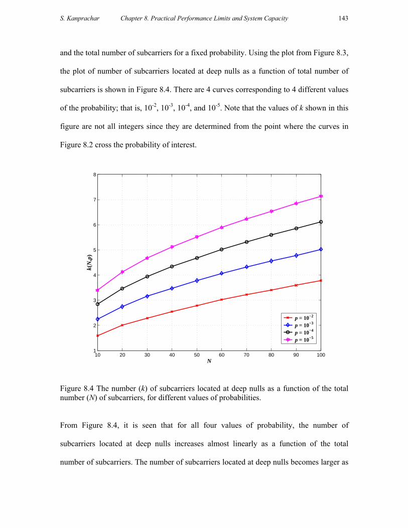
S. Kanprachar Chapter 8. Practical Performance Limits and System Capacity
143
and the total number of subcarriers for a fixed probability. Using the plot from Figure 8.3,
the plot of number of subcarriers located at deep nulls as a function of total number of
subcarriers is shown in Figure 8.4. There are 4 curves corresponding to 4 different values
of the probability; that is, 10-2, 10-3, 10-4, and 10-5. Note that the values of k shown in this
figure are not all integers since they are determined from the point where the curves in
Figure 8.2 cross the probability of interest.
10 20 30 40 50 60 70 80 90 1001
2
3
4
5
6
7
8
N
k(N
,p)
p = 10−2
p = 10−3
p = 10−4
p = 10−5
Figure 8.4 The number (k) of subcarriers located at deep nulls as a function of the total number (N) of subcarriers, for different values of probabilities.
From Figure 8.4, it is seen that for all four values of probability, the number of
subcarriers located at deep nulls increases almost linearly as a function of the total
number of subcarriers. The number of subcarriers located at deep nulls becomes larger as

S. Kanprachar Chapter 8. Practical Performance Limits and System Capacity
144
the probability of interest decreases. It should be noted that the probabilities used in this
figure are chosen arbitrarily so some probabilities may not be useful for system design. It
is of interest to determine which of these probabilities is really useful.
From the simulation results in Chapter 6, it is seen that the system performance (in
terms of bit-error-rate (BER)) for a 10-subcarrier system using a training process
(dropping 2 channels) is good for all five sets of multimode fiber. This implies that for a
10-subcarrier system the maximum number of subcarriers located at deep nulls is not
greater than 2. And, the BERs for the system with a larger number of subcarriers using a
training process (dropping 2 channels) are not low for all five sets of multimode fiber.
This means that with a larger number of subcarriers, the number of subcarriers located at
deep nulls can be larger than 2 subcarriers. Using this information with the curves shown
in Figure 8.4, it is seen that the curves from using probabilities of 10-4 and 10-5 are
pessimistic since the number of subcarriers located at deep nulls from these two curves
for N = 10 are 2.8 and 3.4, which is larger than 2. And, the curve from the probability of
10-2 is slightly optimistic since for N = 20 and 30, the numbers of subcarriers located at
deep nulls are 2 and 2.3, which are close to 2. Considering the curve from the probability
of 10-3, it is seen that for N = 10, the number of subcarriers located at deep nulls is 2.2,
and for N = 20, 30, and 40, the numbers of subcarriers located at deep nulls are 2.8, 3.2,
and 3.5. The information from the curve with a probability of 10-3 agrees with the
simulation results. Note that the simulation results were done with 5 different fiber
responses, which were chosen to have generally poor response. This means that even
though only 5 fiber responses were studied, the curve from the probability of 10-3 can be

S. Kanprachar Chapter 8. Practical Performance Limits and System Capacity
145
reasonably used for approximating the number of subcarriers that are located at deep
nulls for a given N.
Another important conclusion that can be drawn from this figure is the total bit rate
that can be used in the system. It is seen that if the system complexity and the bandwidth
limited by chromatic dispersion are not taken into account, the total bit rate can be as
high as we want just by increasing the number of subcarriers since it is assumed that each
subcarrier signal carries a fixed bit rate; that is, one-half of the intermodal bandwidth.
However, a high bit rate may not be feasible since when the number of subcarriers
increases, the number of subcarriers located at deep nulls also increases. To get good
system performance with a large number of subcarriers located at deep nulls, system
complexity becomes an important factor since the system will certainly need more
channels to be dropped for a training process or more complex diversity coding in order
to recover the data from all good channels. Moreover, with a larger number of
subcarriers, the bandwidth required for transmitting the signal becomes larger. This large
bandwidth may exceed the bandwidth limited by chromatic dispersion, or it may be larger
than that achievable with practical electronics. Therefore, it is seen that the total bit rate is
not unlimited. It is limited by the system complexity and the available bandwidth limited
by chromatic dispersion and practical circuit considerations. For example, if it is assumed
that the bandwidth required by the total bit rate does not exceed the bandwidth limited by
chromatic dispersion, and the system can recover the data if up to 5 subcarriers are
located at deep nulls (this is determined from the curve with the probability of 10-3 in

S. Kanprachar Chapter 8. Practical Performance Limits and System Capacity
146
Figure 8.4), then the total number of subcarriers can be up to 100, resulting in a total bit
rate of 5 Gbps (i.e., 100×0.5×BWintermodal = 100×0.5×100 MHz = 5 Gbps).
In summary, the probability of having k subcarriers (from an N-subcarrier system)
located at deep nulls has been discussed in this section. The probability has been shown
for different numbers of k and N. It has been seen that for a fixed N, the probability
decreases as k increases. And, for a fixed k, the probability increases as N increases. Plots
relating the number of deep nulls and the total number of subcarriers for different values
of probabilities have also been shown. It is found that the relationship between k and N
using a fixed probability of 10-3 is suitable for system consideration since the information
from this curve agrees with the simulation results done previously. The total bit rate of
the system can also be determined from this curve if other factors (i.e., system
complexity and bandwidth limitation from chromatic dispersion) are not considered.
8.3.3 Number of subcarriers located at the deep nulls from Poisson distribution
The probability of having k subcarriers (from an N-subcarrier system) located at deep
nulls (10 dB below the average amplitude) has been discussed in the previous section.
The number of subcarriers located at deep nulls for different values of probability has
been shown. It was shown that the curve between k and N with the probability of 10-3
agrees with the simulation results in Chapter 5 to 7. Also, using the probability of 10-3 is
reasonable since it can then be interpreted that only 0.1% of multimode fibers might be

S. Kanprachar Chapter 8. Practical Performance Limits and System Capacity
147
expected to give unsatisfactory performance. The data used in Figure 8.4 is from the
numerical calculation using the binomial distribution. It is seen that for large N the
number k is very small compared to the value of N. And, the probability that the
amplitude of the response of the multimode fiber at a particular frequency is less than 10
dB below the average amplitude is very small (i.e., 0.0078) as N gets larger. Hence, the
probability of having k subcarriers (from an N-subcarrier system) located at deep nulls
can then be approximated by the Poisson distribution. In this section, the analytic result
for the probability of having k subcarriers (from an N-subcarrier system) located at deep
nulls using the Poisson distribution is studied.
From (8-18), it is seen that as N gets larger, the probability of having k subcarriers
(from an N-subcarrier system) located at deep nulls, which is a Binomial distribution, can
be approximated by a Poisson distribution. For a particular N, the probability of having k
subcarriers (from an N-subcarrier system) located at deep nulls is then given by
( )!
k
P k ek
λ λ−= (8-19)
where λ = ( )( )fiberH fF m Nε × = 0.0078×N.
Using (8-19) with different values of k and N, the probability of having k subcarriers
(from an N-subcarrier system) located at deep nulls can be determined. The plot of this
probability is shown in Figure 8.5 on a logarithmic scale as a function of k. The total
number of subcarriers is varied from 10 to 100.

S. Kanprachar Chapter 8. Practical Performance Limits and System Capacity
148
1 2 3 4 5 6 7 8 9 1010
−6
10−5
10−4
10−3
10−2
10−1
100
P(k
)
k
N = 10N = 20N = 30N = 40N = 50N = 60N = 70N = 80N = 90N = 100
Figure 8.5 Probability of having k subcarriers (from an N-subcarrier system) located at deep nulls (at least 10 dB below the average amplitude) determined from Poisson distribution in (8-19).
Comparing the curves in Figure 8.5 to the curves shown in Figure 8.3 (which is from
the Binomial distribution), it is seen that these curves are almost identical. The difference
becomes smaller as N gets larger. From Figure 8.5, the relationship between the number
of deep nulls and the total number of subcarriers for a fixed probability can be
determined. Setting the probability of interest to be 10-3, the number of subcarriers
located at deep nulls can be plotted as a function of N, as shown in Figure 8.6.

S. Kanprachar Chapter 8. Practical Performance Limits and System Capacity
149
10 20 30 40 50 60 70 80 90 1002
2.5
3
3.5
4
4.5
5
5.5
N
k(N
,p)
Binomial Dist., p = 10−3
Poisson Dist., p = 10−3
Figure 8.6 The number (k) of subcarriers located at deep nulls as a function of the total number (N) subcarriers: from Binomial and Poisson distributions, p = 10-3.
From Figure 8.6, it is seen that there are two curves corresponding to Binomial
distribution and Poisson distribution. The number of subcarriers located at deep nulls
increases as the number of total subcarriers increases. For a large N, the number of
subcarriers located at deep nulls increases almost linearly as a function of the total
number of subcarriers. Comparing these two curves, it is clearly seen that they are almost
identical. The gap between these two curves is very small, approximately 0.05. This then
shows that instead of using a Binomial distribution, the probability of having k
subcarriers (from an N-subcarrier system) located at deep nulls can also be determined by
using the Poisson distribution, which requires less calculation.

S. Kanprachar Chapter 8. Practical Performance Limits and System Capacity
150
To show how the number of subcarriers located at deep nulls increases as a function
of N, the ratio between k and N has to be determined. This ratio, as determined from the
results in Figure 8.6, is plotted as a function of N in Figure 8.7.
10 20 30 40 50 60 70 80 90 1000.04
0.06
0.08
0.1
0.12
0.14
0.16
0.18
0.2
0.22
0.24
N
k(N
,p)
/ N
Binomial Dist., p = 10−3
Poisson Dist., p = 10−3
Figure 8.7 The ratio between the number (k) of subcarriers located at deep nulls and the total number (N) of subcarriers as a function of the total number subcarriers: from Binomial and Poisson distributions, p = 10-3.
Two curves are shown in Figure 8.7. These two curves are for the Binomial
distribution and Poisson distribution and they are almost the same. It is seen that for small
N, the parameter k/N is high. And, when N increases, k/N becomes smaller and reaches
0.05 at N = 100. This means that as N increases, the number of subcarriers located at deep
nulls increases almost linearly as a function of N since k/N approaches a constant. Hence,

S. Kanprachar Chapter 8. Practical Performance Limits and System Capacity
151
the number of subcarriers located at deep nulls can be estimated easily if the total number
of subcarriers is known.
An analytic result, approximating the probability of having k subcarriers (from an N-
subcarrier system) located at deep nulls, using a Poisson distribution has been given in
this section. Plots of k and k/N as a function of N have been shown. It has been seen that
as N gets larger, k increases almost linearly as a function of N. This is very useful since
the number of subcarriers located at deep nulls can then be easily approximated if the
total number of subcarriers is known.
8.4 System Capacity
The available bandpass bandwidth limited by chromatic dispersion and the
probability of having k subcarriers (from an N-subcarrier system) located at deep nulls
(which have an amplitude less than 10 dB below the average amplitude of the frequency
response of multimode fiber) has been analyzed. The result of this analysis shows that the
bandpass bandwidth, which seems to be unlimited if only modal dispersion is taken into
account, is limited by chromatic dispersion. From the analysis of the probability of
having k subcarriers (from an N-subcarrier system) located at deep nulls, it is seen that
the number of subcarriers located at deep nulls increases as the total number of
subcarriers increases. Also, the probability of having k subcarriers (from an N-subcarrier

S. Kanprachar Chapter 8. Practical Performance Limits and System Capacity
152
system) located at deep nulls can be determined approximately by the Poisson
distribution. However, a major system question still remains. What is the total bit rate
that may be achieved, and how does this depend on transmitter power and fiber length?
In this section, these questions are considered, and a plot relating total bit rate and fiber
length will be obtained, making use of the results from previous sections of this chapter.
For optical fiber transmission, the electrical transmitted signal must be converted into
an optical format using an optical source. As has been discussed in the previous section,
vertical cavity surface-emitting lasers (VCSELs) are suitable for SCM multimode fiber
systems. To operate the laser in the stimulated emission region, the laser must be driven
by a bias current (IB), which must be higher than the threshold current (Ith). This bias
current results in a DC component at the output optical signal of the laser. The fluctuation
(∆I) in the drive current about the bias point is caused by the transmitted signal. This
fluctuation in the drive current then results in an AC component of the output optical
signal of the laser. For an N-subcarrier system, the transmit optical power in the DC and
AC components are given by
,, ,
12
T OpticalT Optical DC
carrier
PP
Nm=
+ (8-20)
and, ,
, ,2
12
carrierT Optical
T Optical ACcarrier
NP mP
Nm=
+ (8-21)
where PT,Optical is the total transmit optical power.
PT,Optical,DC is transmit optical power in DC component

S. Kanprachar Chapter 8. Practical Performance Limits and System Capacity
153
PT,Optical,AC is transmit optical power in AC component (i.e., all subcarrier signals)
Ncarrier is the total number of subcarriers
m is the modulation index for each subcarrier signal, which is assumed to be
identical for all subcarriers. Note that the definition of the modulation index was given in
Chapter 5. From [34], m is given by
2
carrier
mN
µ= (8-22)
µ is the total rms modulation index.
From (8-22), the maximum subcarrier modulation index (m) depends on the allowable
µ and the number of subcarriers Ncarrier. If µ is fixed as a constant, m will depend only on
Ncarrier. Ncarrier depends on many parameters; that is, the available bandpass bandwidth
(BBP), the bit rate per subcarrier (Rb,sub), and the spacing between two successive
subcarriers (∆fsub). Ncarrier is given by
,
BPcarrier
sub b sub
BNf R
=∆
(8-23)
It was shown in Chapter 2 that the bit rate for each subcarrier should be less than one-
half of the 3-dB modal bandwidth (B3-dB,modal) of the multimode fiber in order to reduce
the effect of signal variation caused by the frequency response of the multimode fiber in
the bandpass region. Hence, in this section, the bit rate per subcarrier will be assumed to
be equal to one-half of B3-dB,modal; that is,
3 ,mod, 2
dB alb sub
BR −= (8-24)

S. Kanprachar Chapter 8. Practical Performance Limits and System Capacity
154
where 3 ,modFiber
dB alBWLB
L− = (8-25)
BWLFiber is the 3-dB modal bandwidth–distance product of the multimode fiber
L is the fiber length.
Note that in (8-25), it is assumed that bandwidth scales inversely with length; i.e., there is
no mode mixing.
From (8-23) and (8-24), the total bit rate (Rb) is given by
Rb = Rb,subNcarrier (8-26)
Passing this subcarrier multiplexed signal through the multimode fiber, the signal
power in the DC and AC components will be attenuated by the fiber attenuation and
attenuation from the passband region of the multimode fiber. The received optical power
at the end of the multimode fiber is then given by
,, ,
12
T OpticalR Optical DC Fiber
carrier
PP Loss
Nm= ×
+ (8-27)
,
, ,2
12
carrierT Optical
R Optical AC Fiber BPcarrier
NP mP Loss Loss
Nm= × ×
+ (8-28)
Fiber FiberLoss Lα= × (8-29)
mod4BP
e
LossNπ
= (8-30)
where PR,Optical,DC is received optical power in the DC component
PR,Optical,AC is received optical power in the AC component (i.e., all subcarrier
signals)

S. Kanprachar Chapter 8. Practical Performance Limits and System Capacity
155
LossFiber is the attenuation of the multimode fiber
LossBP is the attenuation from transmitting signal in bandpass region
αFiber is the multimode fiber attenuation coefficient
Nmode is the number of guided modes supported by the multimode fiber.
From (8-27) and (8-28), it is seen that the power of the DC component is only
affected by the attenuation from the multimode fiber while the power of AC component
is affected by the attenuations from the multimode fiber and the bandpass region since the
AC component is transmitted over the bandpass region of the fiber. Hence, the AC
component is attenuated significantly. Note that LossBP given in (8-30) is the average
attenuation caused by the high frequency region of the fiber. Hence, the power of the AC
component shown in (8-28) is the average power. The received optical signal is sent to
the photodetector, in which the received optical signal will be converted to an electrical
signal as a photocurrent. The photocurrent for DC and AC components (i.e., IR,DC and
IR,AC) are given by
, , ,R DC R Optical DCI P= R (8-31)
and , , ,R AC R Optical ACI P= R (8-32)
where R is the responsitivity of the photodetector.
From (8-32), it is seen that the average electrical power of all received subcarrier
signals (PR,Elec,AC) and the average electrical power of each received subcarrier signal
(PR,Elec,sub) are given by
( )22, , , , ,R Elec AC R AC R Optical ACP I P= = R (8-33)

S. Kanprachar Chapter 8. Practical Performance Limits and System Capacity
156
( )2
, ,, ,, ,
R Optical ACR Elec ACR Elec sub
carrier carrier
PPP
N N= =
R (8-34)
To calculate the signal-to-noise ratio of the received subcarrier signal, the noise
power has to be determined. It is assumed that thermal noise is dominant and the
receiver’s optical front end is transimpedance design with an effective noise capacitance
of Ce [41]. The total noise power (PNoise), the noise power in AC portion (PNoise,AC), and
the noise power per subcarrier (PNoise,sub) are given by
28Noise T e eP qV C Bπ= (8-35)
2, 8 BP
Noise AC T e ee
BP qV C BB
π= × (8-36)
2,
18 BPNoise sub T e e
e carrier
BP qV C BB N
π= × × (8-37)
where q is the electron charge (= 1.6 × 10⁻¹⁹ C), BT
k TVq
= = 0.025 V at T = 290 K, kB is
the Boltzmann constant (= 1.38 × 10⁻²³ J/K), T is the absolute temperature, and Be is the
effective noise bandwidth of the receiver.
From (8-34) and (8-37), the signal-to-noise ratio for each subcarrier is given by
( )2
, ,, ,
, 8R Optical ACR Elec sub
Noise sub T e e BP
PPSNR
P qV C B Bπ= =
R (8-38)
For digital signal transmission, the minimum signal-to-noise ratio of the received
signal should be greater than 15 dB in order to get good performance. If the signal-to-

S. Kanprachar Chapter 8. Practical Performance Limits and System Capacity
157
noise ratio in (8-38) is less than SNRreq = 15 dB, the quality of the received signal is not
acceptable and some system parameters have to be modified. If the number of subcarriers
decreases, the power in each subcarrier signal will increase. Consequently, the achieved
SNR will increase. Note that the bit rate per subcarrier is still the same since the fiber
length does not change. Thus, the total bit rate will decrease if the number of subcarriers
decreases.
Another important factor affecting the total bit rate is the number of subcarriers
located at deep nulls. Using the probability of 10-3, the number of subcarriers (from an N-
subcarrier system) located at deep nulls can be determined by solving the following
equation, which was found previously in (8-19); that is,
( )!
k
P k ek
λ λ−= (8-39)
where P(k) is the probability of having k subcarriers located at deep nulls in Ncarrier
subcarriers and λ = 0.0078×Ncarrier for deep nulls.
The number of subcarriers that can successfully transmit the signal to the receiver is
determined by subtracting the number of subcarriers located at deep nulls (determined
from (8-39)) from the total number of subcarriers. Hence, the total bit rate that can be
transmitted to the receiver successfully can be determined.

S. Kanprachar Chapter 8. Practical Performance Limits and System Capacity
158
Next, the results from the discussion above will be used to determine the signal-to-
noise ratio, the number of subcarriers and the total bit rate for given system parameters.
The following system parameters are assumed. The transmit optical power (PT,Optical) is 1
mW. The number of guided modes (Nmode) supported by the multimode fiber is 100
modes. The maximum available bandpass bandwidth (BBP) is 4 GHz. The 3-dB modal
bandwidth–distance product (BWLFiber) of the multimode fiber is 500 MHz-km. The total
rms modulation index (µ) is 0.5. The value of µ seems to be large; however, it was shown
in [34 - 36], using µ = 0.5 is sufficient for a digital system since the carrier to nonlinear
distortion ratio from this µ is greater than 25 dB. The spacing between two successive
subcarriers (∆fsub) is 2.5 times the bit rate per subcarrier (Rb,sub). The fiber attenuation
coefficient (αFiber) is 1 dB/km. The responsitivity (R) of the photodetector is 0.9 A/W.
The effective noise capacitance (Ce) is 1 pF. The rms thermal noise current (referred to
the output of the photodtector) is 2.5 µA. And, the minimum required signal-to-noise
ratio (SNRreq) for each received subcarrier signal is 15 dB. The fiber length (L) is varied
from 0.4 to 6 km. Note that as the fiber length changes, the intermodal bandwidth of the
fiber and hence the bit rate per subcarrier also changes. The plots of received optical
powers, received signal-to-noise ratio as a function of the fiber length will be shown.
Also, the plots of total number of subcarriers and total bit rate as a function of the fiber
length will be given.
From (8-20) to (8-22) the transmit DC and AC powers are given by
,, , 1
T OpticalT Optical DC
PP
µ=
+ (8-40)
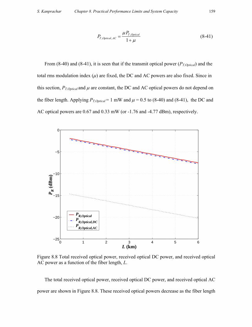
S. Kanprachar Chapter 8. Practical Performance Limits and System Capacity
159
,, , 1
T OpticalT Optical AC
PP
µµ
=+
(8-41)
From (8-40) and (8-41), it is seen that if the transmit optical power (PT,Optical) and the
total rms modulation index (µ) are fixed, the DC and AC powers are also fixed. Since in
this section, PT,Optical and µ are constant, the DC and AC optical powers do not depend on
the fiber length. Applying PT,Optical = 1 mW and µ = 0.5 to (8-40) and (8-41), the DC and
AC optical powers are 0.67 and 0.33 mW (or -1.76 and -4.77 dBm), respectively.
0 1 2 3 4 5 6−25
−20
−15
−10
−5
0
L (km)
PR (
dBm
)
PR,OpticalP
R,Optical,DCP
R,Optical,AC
Figure 8.8 Total received optical power, received optical DC power, and received optical AC power as a function of the fiber length, L.
The total received optical power, received optical DC power, and received optical AC
power are shown in Figure 8.8. These received optical powers decrease as the fiber length

S. Kanprachar Chapter 8. Practical Performance Limits and System Capacity
160
increases since the fiber attenuation increases. From the figure, it is seen that the received
optical DC power is always larger than the received optical AC power. At the receiver,
the difference between the DC and AC powers is approximately 12 dB while at the
transmitter this difference is just 3 dB. The additional decrease in the optical AC power at
the receiver is caused by the attenuation in the bandpass region of the multimode fiber.
This attenuation will affect only the AC portion of the transmit signal; hence, the
received optical AC power becomes much less than the received optical DC power. Note
that from the given system parameters, the number of guided modes supported by the
multimode fiber is 100 modes; thus, the attenuation from sending a signal in the passband
region is 9.5 dB independent of the fiber length.
0 1 2 3 4 5 614
16
18
20
22
24
26
L (km)
SNR
(dB
)
Figure 8.9 The signal-to-noise ratio of the received subcarrier signal as a function of the fiber length, L.

S. Kanprachar Chapter 8. Practical Performance Limits and System Capacity
161
In Figure 8.9, the signal-to-noise ratio of the received subcarrier signal is plotted as a
function of the fiber length. It is seen that for the fiber length less than 5.2 km, the signal-
to-noise ratio decreases as the fiber length increases. This is the effect of the fiber
attenuation, which increases as a function of the fiber length. However, for the fiber
length greater than 5.2 km, the number of subcarriers has to be decreased in order to keep
the signal-to-noise ratio above the minimum required signal-to-noise ratio, which is 15
dB. Therefore, for the fiber length greater than 5.2 km, the signal-to-noise ratio is slightly
above 15 dB. The effect of keeping signal-to-noise ratio above 15 dB will be shown by
the number of subcarriers and the total bit rate shown in Figure 8.10 and 8.11.
0 1 2 3 4 5 60
5
10
15
20
25
30
35
L (km)
Nca
rrie
r
Including possible deep nullsNot including possible deep nulls
Figure 8.10 The number of subcarriers as a function of the fiber length.

S. Kanprachar Chapter 8. Practical Performance Limits and System Capacity
162
The number of subcarriers for different fiber lengths is shown in Figure 8.10. There
are two curves in this figure; that is, the number of subcarriers calculated from (8-23) and
the number of subcarriers calculated from (8-23) subtracted by the number of possible
deep nulls. For the fiber length below 5.2 km, the number of subcarriers from these two
curves increases as the fiber length increases. This is because as distance increases, fiber
bandwidth decreases, and the bit rate per subcarrier decreases. The difference of number
of subcarriers between these two curves increases as the fiber length increases since the
number of possible subcarriers located at deep nulls increases as the total number of
subcarriers increases. For a fiber length greater than 5.2 km, the number of subcarriers
from these two curves decreases. This is the effect from keeping the signal-to-noise ratio
of the received subcarrier signal above the minimum required signal-to-noise ratio by
decreasing the number of subcarriers. The decrease of the number of subcarriers will
certainly affect the total bit rate. This is shown in Figure 8.11.

S. Kanprachar Chapter 8. Practical Performance Limits and System Capacity
163
0 1 2 3 4 5 6600
700
800
900
1000
1100
1200
1300
1400
1500
L (km)
Rb
(Mbp
s)
Figure 8.11 The total bit rate as a function of the fiber length.
The total bit rate as a function of the fiber length is shown in Figure 8.11. The curve
shown in Figure 8.11 corresponds to the total bit rate from subcarriers that are not located
at deep nulls. That is, it is assumed that the effects of having some subcarriers located at
the deep nulls are overcome by some system modifications; for example, training process
or diversity coding. Note that the reasons for the fluctuation of this curve will be
discussed later. It is seen that for the fiber length below 5.2 km, the total bit rate increases
as the fiber length increases. At a fiber length less than 2.2 km, the total bit rate strongly
increases as a function of the fiber length. This can be explained as follows. For a short
fiber length, the bit rate per subcarrier is large because the intermodal bandwidth is large,
and the total number of subcarriers (Ncarrier) is then small. Discarding only one or two

S. Kanprachar Chapter 8. Practical Performance Limits and System Capacity
164
subcarriers located at deep nulls will significantly decrease the total bit rate. And, as the
fiber length increases; the bit rate per subcarrier decreases, Ncarrier increases, and the
number (k) of subcarriers located at deep nulls increases. However, the increase of k is
much less than the increase of Ncarrier. For example, for Ncarrier = 10, k = 2 while for
Ncarrier = 20, k = 3. And, since the bit rate per subcarrier is small, discarding a small
number of subcarriers (which are located at deep nulls) from a large Ncarrier will not
significantly decrease the total bit rate of the system. Hence, as the fiber length increases,
the total bit rate increases.
It is seen that for a fiber length below 2 km the total bit rate is low compared to the
total bit rate at longer distances. Generally, it is expected that the total bit rate should be
high at a short distance. It is not true in this system as seen from Figure 8.11. This is
because the total number of subcarriers is determined by the bit rate per subcarrier, which
is assumed to be one-half of the 3-dB modal bandwidth (B3-dB,modal) for a particular fiber
length (see (8-23) and (8-24)). For a short fiber length, the 3-dB modal bandwidth is large
(e.g., at L = 1.0 km, B3-dB,modal = 500 MHz), the bit rate per subcarrier is then high; hence,
the total number of subcarriers is small. This small number of subcarriers is the minimum
number of subcarriers to be used so that each subcarrier signal will not experience large
amplitude variation from the frequency response of the fiber. However, with a small
number of subcarriers, the total bit rate is then considerably reduced if only one or two
subcarriers are ignored. To increase the total bit rate for the system at such short distance,
it is possible to decrease the bit rate per subcarrier; that is, there will be many subcarriers
in one passband region. Hence, the total number of subcarriers used in the system will

S. Kanprachar Chapter 8. Practical Performance Limits and System Capacity
165
increase. This will then lessen the effect of discarding some subcarriers located at deep
nulls. From Chapters 5-7, it is seen that a 10-subcarrier system gives good system
performance. Also, the number of subcarriers in a 10-subcarrier system is not too large;
that is, the system complexity is not a problem. Therefore, if the minimum number of
subcarriers of the system is set to be 10, the total bit rate at short distances should
increase. For example, at L = 0.9 km, with Ncarrier = 10, the total bit rate is 1,280 Mbps.
Note that, with Ncarrier = 10, the bit rate per subcarriers is 160 Mbps and the number of
subcarriers located at deep nulls is 2. Comparing this total bit rate to the total bit rate
(which is 830 Mbps) at L = 0.9 km shown in Figure 8.11, it is seen that limiting the total
number of subcarriers to be at least 10 subcarriers can increase the total bit rate.
From Figure 8.11 there are some fluctuations in the total bit rate as the fiber length
increases. This can be explained as follows. In Figure 8.10, it is seen that the number of
subcarriers does not always increase as the fiber length increases. There is a situation
where the numbers of subcarriers from two fiber lengths are identical. To determine the
total bit rate, this number of subcarriers has to be multiplied by the bit rate per subcarrier.
Since the bit rate per subcarrier from the longer fiber is less than the bit rate per
subcarrier from the shorter fiber, the total bit rate from the longer fiber is then less than
the total bit rate from the shorter fiber. Considering the total bit rate curve in Figure 8.11,
there are two points where the decrease of total bit rate is significant; that is, at L = 0.9
and 2.4 km. At these two fiber lengths, the number of subcarriers located at deep nulls
increases from 1 to 2 and from 2 to 3, respectively. This results in a smaller number of
subcarriers that are not located at deep nulls; thus, the lower total bit rate. For the fiber
S. Kanprachar Chapter 8. Practical Performance Limits and System Capacity
166
length greater than 5.2 km, the total bit rate decreases rapidly as the fiber length
increases. The reason for this was explained previously as a consequence of keeping the
signal-to-noise ratio of the subcarrier signal above the minimum required signal-to-noise
ratio. Note that the maximum total bit rate is approximately 1,450 Mbps, which is at L =
5.2 km. This bit rate is approximately 15 times larger than the bit rate of the signal
transmitted over the 3-dB modal bandwidth of the same fiber length. From this figure, it
is seen that the system is not bandwidth-limited but noise-limited. If the transmit optical
power increases, the higher total bit rate can then be achieved.
In this section, the relationships between many system parameters (e.g., signal-to-
noise ratio, number of subcarriers, total bit rate, and fiber length) are discussed. The DC
and AC optical powers at the transmitter are assumed constant since the transmitter
power and the total rms modulation index are fixed. The DC and AC optical powers at
the receiver decreases as the fiber length increases. This is the effect of the fiber
attenuation. As the fiber length increases, the 3-dB modal bandwidth of the fiber
decreases and the bit rate per subcarrier decreases. This then leads to an increase in the
total number of subcarriers since the maximum available bandpass bandwidth of the fiber
is fixed. As the total number of subcarriers increases, the signal power per sucarrier
decreases; hence, the signal-to-noise ratio of the received subcarrier signal decreases.
That is, the signal-to-noise ratio of the received subcarrier signal decreases as the fiber
length increases. However, the signal-to-noise ratio should not be below the minimum
required signal-to-noise ratio since if it is below the minimum required signal-to-noise
ratio, the received signal performance will be poor; thus, large bit-error rate will be

S. Kanprachar Chapter 8. Practical Performance Limits and System Capacity
167
achieved. To keep the signal-to-noise ratio above the minimum level, the number of
subcarriers must decrease. This then increases the power in each subcarrier signal.
However, the total bit rate will decrease because the number of subcarriers decreases.
There is a maximum fiber length that can give a high total bit rate. If the fiber length is
longer than this maximum length, the total bit rate will not further increase but decrease
rapidly. It is seen that the multimode fiber system using subcarrier multiplexing is not
bandwidth-limited but noise-limited. A higher bit rate can be achieved if the transmit
optical power increases.
8.5 Conclusions
The performance limits and system capacity of the SCM multimode fiber system have
been analyzed in this chapter. The effect of the chromatic dispersion on the available
bandpass bandwidth has been discussed. It is seen that the available bandpass bandwidth
of a multimode fiber is limited by the chromatic dispersion. It is shown that the maximum
bandpass bandwidth-distance product up to 500 GHz⋅km can be achieved if the 1300-nm
operating wavelength and a VCSEL with a spectral width of 0.5 nm are used. The effects
of having some subcarriers located at the nulls of multimode fiber were also analyzed. It
was found that as the total number of subcarriers increases, the number of subcarriers
located at the nulls of multimode fiber increases. Three levels of nulls were considered;
that is, 3, 5, and 10 dB below the average amplitude of the magnitude response of the
multimode fiber at high frequencies. Having some subcarriers located at the shallow

S. Kanprachar Chapter 8. Practical Performance Limits and System Capacity
168
nulls, which are 3 or 5 dB below the average amplitude, does not significantly degrade
the received signal quality since the received signal is not strongly attenuated by the
nulls. Hence, the effect of these nulls on the received signal should be small. On the other
hand, for the case of deep nulls (whose amplitude is lower than 10 dB below the average
amplitude), having some subcarriers located at these nulls will certainly degrade the
quality of the received signal. It has been shown that the probability of having some
subcarriers located at the nulls of multimode fiber can be described by the Binomial
distribution, as shown in (8-17). And, for the case of deep nulls, this probability can also
be approximated by the Poisson distribution, as shown in (8-19). Curves relating the
number of subcarriers located at deep nulls, and the total number of subcarriers for
different values of probability, have been presented. Comparing these curves to the
results found in Chapter 6 and 7, it is seen that the curve with a probability of 10-3 is the
most suitable for predicting the relationship between the number of subcarriers located at
deep nulls and the total number of subcarriers in the system. Using the information from
this curve, the system capacity of the SCM multimode fiber system has been discussed.
The total bit rate up to 1.45 Gbps can be achieved for the fiber length of 5.2 km. The high
total bit rate cannot be achieved at shorter distances (with the assumptions made in the
analysis) since the bit rate per subcarrier is large and the total number of subcarriers is
small. To increase the total bit rate at the fiber length below 2 km, a minimum total
number of subcarriers should be set. That is, if the total number of subcarriers determined
from (8-23) is smaller than the minimum, it will be set to be identical to the minimum
and the bit rate per subcarrier will be decreased. It has been shown that the total bit rate at
short distances increases if the minimum total number of subcarriers is set to be 10. For

S. Kanprachar Chapter 8. Practical Performance Limits and System Capacity
169
the fiber length greater than 5.2 km, the total bit rate decreases rapidly. This is the
consequence of having the achieved SNR below the minimum required SNR. It is seen
that the system is not bandwidth-limited but noise-limited. If the transmit optical power
increases, the higher total bit rate can then be achieved. The maximum fiber length, the
maximum bit rate, and the number of subcarriers for different transmit optical powers are
shown in Table 8.1.
Table 8.1 List of the maximum fiber length, the maximum bit rate, and the number of
subcarriers for different values of transmit optical power
PT (mW) Lmax (km) Rb,max (Gbps) Ncarrier 0.5 2.2 1.36 14 1 5.2 1.45 33 2 8.3 1.47 52 5 12.1 1.5 78 10 15.2 1.52 97
From Table 8.1, it is seen that the maximum bit rate increases only slightly as the
transmit optical power increases, but the maximum distance increases significantly. One
disadvantage of the system with higher power and longer distance is that the number of
subcarriers is very large as seen from the table. Since the higher maximum bit rate is
achieved from the system with a longer fiber length, the bit rate per subcarrier of such
system is very small. Hence, more subcarriers are needed in order to cover all available
passband bandwidth. This then means that to get longer distance and higher maximum bit
rate, more system complexity is needed.

S. Kanprachar Chapter 9. Summary and Conclusions 170
Chapter 9
Summary and Conclusions
In this dissertation, the frequency response of multimode fiber at high frequencies is
analyzed. Different transmission approaches for sending the signal via this high
frequency region and the resulting system performance are studied. To improve the
performance of the SCM multimode fiber system, two types of system modifications are
studied; that is, a training process and diversity coding. The practical limits and capacity
of the SCM multimode fiber system are presented.
From the analysis of the passband region of multimode fiber, the impulse response of
the complex envelope of the fiber is modeled as the combination of delta functions
corresponding to different delays. With this model, the probability density function of the
magnitude response of the fiber at high frequencies is a Rayleigh density function. The
magnitude response of the fiber at high frequencies does not fall off monotonically as the
frequency increases, but becomes relatively flat with many nulls. The average amplitude
of this flat region does not depend on the frequency but depends on the number of guided
modes supported by the fiber. Also, the available bandwidth of each passband region is
comparable to the intermodal bandwidth of the fiber.

S. Kanprachar Chapter 9. Summary and Conclusions 171
To transmit a signal over the high frequency region of multimode fiber, many
transmission approaches are studied in this dissertation. It has been shown that adding an
electrical equalizer at the receiver in order to compensate the attenuation caused by the
amplitude variation in the passband region of the fiber is not a good approach since the
noise can be significantly amplified. The effect of using direct sequence spread spectrum
is also studied. It has been shown that the standard deviation of the signal-to-noise ratio
of the received signal decreases as the code length increases. However, the average
signal-to-noise ratio of the received signal also decreases as the code length increases.
This is because the phase information of the received optical signal is totally discarded by
the non-coherent receiver. As a result, the power of the received decoded signal is not
improved. However, as the code length increases, the required bandpass bandwidth
increases, and consequently the noise power increases. Therefore, using direct sequence
spread spectrum with passband transmission on multimode fiber is not a good choice.
The system performance of the multimode fiber system using subcarrier multiplexing
has been studied. A high bit rate signal is divided into many low bit rate signals. These
low bit rate signals are then modulated onto different subcarrier frequencies. With this
approach, the frequency response of multimode fiber, which is a wideband frequency-
selective channel, is transformed into a series of many narrowband frequency-
nonselective channels. It has been shown that a 500-Mbps signal can be transmitted over
the passband region of multimode fiber. The effect of the number of subcarriers has also
been studied. For a fixed total bit rate, with a large number of subcarriers, the bit rate per
subcarrier becomes small resulting in less signal variation caused by the fiber. However,

S. Kanprachar Chapter 9. Summary and Conclusions 172
with this large number of subcarriers, the probability that some subcarriers are located at
deep nulls of the fiber becomes high. And, these subcarriers located at deep nulls can
significantly degrade the system performance.
To improve the system performance of the SCM multimode fiber system; that is, to
cancel the effect of having some subcarriers located at deep nulls, a training process and
diversity coding are studied. It has been shown that both techniques can improve the
system performance. However, diversity coding requires less system complexity since the
extra circuit for sending information about the channels’ property back to the transmitter
and extra subcarriers are not needed. Hence, diversity coding is a very powerful
technique for canceling the effects of having some subcarriers located at the deep nulls of
the magnitude response of multimode fiber.
The practical limits and capacity of the SCM multimode fiber system are studied. For
the available passband bandwidth of the fiber, it has been shown that the passband
bandwidth is limited by chromatic dispersion. The probability of having some subcarriers
located at deep nulls of the fiber is studied. This probability is a Binomial distribution
and, for the case of deep nulls, can be approximated by the Poisson distribution. It has
been shown analytically for a given probability the number of subcarriers located at deep
nulls for the case of a large number of subcarriers is large. Making reasonable
assumptions, it has been shown that a 1.45-Gbps signal can be transmitted over a 5-km
multimode fiber. It is found that the SCM multimode fiber system is not bandwidth-
limited but noise-limited.
S. Kanprachar Chapter 9. Summary and Conclusions 173
9.1 Summary of Contributions
The following contributions to the field of multimode fiber transmission systems have
been made as an outcome of the research in this dissertation: (1) the statistical properties
of the frequency response of multimode fiber at high frequencies are analyzed [18, 42],
(2) the performance of the SCM multimode fiber system for different number of
subcarriers is presented [42], (3) the system performance of the SCM multimode fiber
system with a training process, which is used for canceling the effect of having some
subcarriers located at deep nulls, is studied [42, 43], (4) diversity coding, which requires
less system complexity than the training process, is proposed and shown to be a powerful
technique for canceling the effect of the deep nulls in SCM multimode fiber system [42,
43], and (5) the practical limits and system capacity of the SCM multimode fiber system
are analyzed [43].
9.2 Suggestions for Future Research
In this dissertation, it is assumed that the optical carrier is a perfect sinusoid.
However, practical sources have finite linewidth (phase noise) and the effect of this noise
on the response of the fiber should be investigated. This type of noise can also degrade
the system performance. It should be useful to understand the effect of the laser phase
noise on the SCM multimode fiber system. Hence, the study about the laser phase noise
on the SCM multimode fiber could be an interesting future research topic. Another

S. Kanprachar Chapter 9. Summary and Conclusions 174
interesting topic is to include the modal effects and chromatic dispersion to the response
of the fiber. That is, a more precise model of the multimode fiber should be studied.
Measurement of frequency response of the fiber is another topic that can be done. The
analytical model can be compared to the results from the measurement and determine
how well it agrees with the measurement.

S. Kanprachar Appendix A. Effect of the bandwidth of bandpass filter (or the bandwidth of electrical equalizer) on the received SNR
175
Appendix A
Effect of bandwidth of bandpass filter (or the bandwidth of
electrical equalizer) on the received signal-to-noise ratio
The effect of the bandwidth of bandpass filter (or the bandwidth of electrical
equalizer) on the signal-to-noise ratio of the received signal studied in Chapter 3 is
presented here. Varying the bandwidth of the bandpass filter and/or the bandwidth of the
electrical equalizer from 1.5Rb to 4Rb, SNRout and SNRout,Eq at different fsubcarrier are
determined. The plots of SNRout and SNRout,Eq are given in Figure A.1 and A.2.
1.5 2 2.5 3 3.5 410
15
20
25
fsub = 0.5 GHzSN
Rou
t
No EqualizationWith Equalization
1.5 2 2.5 3 3.5 410
15
20
25
fsub = 1 GHzSN
Rou
t
No EqualizationWith Equalization
1.5 2 2.5 3 3.5 415
20
25
30
fsub = 1.5 GHzSN
Rou
t
No EqualizationWith Equalization
1.5 2 2.5 3 3.5 415
20
25
CombinedversionSN
Rou
t
Bandwidth of Bandpass Filter /Rb
No EqualizationWith Equalization
Figure A.1 Signal-to-noise ratio as a function of the bandwidth of bandpass filter: for different subcarriers.

S. Kanprachar Appendix A. Effect of the bandwidth of bandpass filter (or the bandwidth of electrical equalizer) on the received SNR
176
1.5 2 2.5 3 3.5 415
20
25
30
Bandwidth of Bandpass Filter /Rb
SNR
out (
in d
B)
fsub
=0.5 GHzfsub
=1.0GHzfsub
=1.5 GHz
Combined version
1.5 2 2.5 3 3.5 410
15
20
25
30
Bandwidth of Electrical Equalizer /Rb
SNR
out,
Eq (
in d
B)
fsub
=0.5 GHzfsub
=1.0GHzfsub
=1.5 GHz
Combined version
Figure A.2 Signal-to-noise ratio as a function of the bandwidth of bandpass filter (or the bandwidth of electrical equalizer): without and with electrical equalization.
In Figure A.1, the plots of SNRout and SNRout,Eq for different subcarriers are presented.
For each subcarrier signal, it is seen that equalization results in a reduction in the output
signal-to-noise ratio. This reduction depends on the subcarrier frequency (i.e., the
frequency response of the multimode fiber) and the bandwidth of the equalizer. For
example, at fsubcarrier = 0.5 GHz, a large SNR reduction is from the case of small BWBP
(e.g., 1.5Rb) while a smaller SNR reduction is from the case of large BWBP (e.g., 4Rb).
This can be explained by using the plot of the magnitude response of the multimode fiber.
It is seen from Figure 3.2 that there is a large attenuation at the frequency at 0.52 GHz.
And, at this frequency the signal power is not large compared to those at fsubcarrier and
fsubcarrier ± Rb. It means that there will be a large gain from the electrical equalizer at this

S. Kanprachar Appendix A. Effect of the bandwidth of bandpass filter (or the bandwidth of electrical equalizer) on the received SNR
177
frequency. With a small BWBP (e.g., at 1.5Rb), the large signal components at fsubcarrier ±
Rb will be rejected while the thermal noise at the frequency of 0.52 GHz will be strongly
amplified. This then results in a small SNRout,Eq. On the other hand, if the bandwidth of
the equalizer increases (e.g., at 4Rb), the large signal components at fsubcarrier ± Rb will be
included and these two large signal components will increase the signal power; thus, a
larger SNRout,Eq. Note that the larger bandwidth of the electrical equalizer, the more
thermal noise introduced to the output signal. However, for the case of combined version,
SNRout,Eq is better than SNRout as seen from the plot.
In Figure A.2, the signal-to-noise ratios are also plotted as a function of the
bandwidth of the bandpass filter (or the bandwidth of the equalizer). The signal-to-noise
ratio from the system without equalization is shown in the upper plot and the signal-to-
noise ratio from the system with equalization is shown in the lower plot. It is seen that for
the system without equalization, SNRout of the combined signal is less than SNRout from
individual subcarrier signal. While, for the system with equalization, SNRout,Eq of the
combined signal is greater than SNRout,Eq from individual subcarrier signal. The
improvement of the combined signal for the system with equalization and the degradation
of the combined signal for the system without equalization can be explained as follows.
For the case of using equalization, considering only the signal component (not
considering the noise), the signal at each fsubcarrier is equalized and has a shape that is
close to the shape of the input signal. Also, the equalized signals are almost in-phase to
one another; thus, when these three signals are combined, the signal strength of the
combined signal can be three times larger than the signal strength from one subcarrier

S. Kanprachar Appendix A. Effect of the bandwidth of bandpass filter (or the bandwidth of electrical equalizer) on the received SNR
178
signal. And, the total power of the combined signal is approximately increased by 9.5 dB
maximum (from 10log10[32]); however, this maximum increase rarely happens since the
equalized signals are not totally in-phase. Considering the noise component of each
equalized signal, it is seen that thermal noise in this case is strongly amplified since the
frequency response of the equalizer is not flat. When the noise from three subcarrier
signals is combined, the total noise power is just the linear sum of the noise powers from
three signals. Comparing the total signal power to the total noise power for the case of
using equalization, it is clearly seen that SNRout,Eq of the combined signal can be larger
than SNRout,Eq of the individual subcarrier signal as seen from the lower plot of SNRout,Eq
for different cases in Figure A.2.
For the case of without equalization, considering only the signal component (not
considering the noise), depending of the frequency response of the multimode fiber, the
shape of the individual subcarrier signal can be almost like the shape of input signal.
However, since the signal at each fsubcarrier is not equalized, the phases of these subcarrier
signals are not in-phase. When three different subcarrier signals are combined, there is no
guarantee that these signals will increase the signal strength of the combined signal. They
may also cancel one another and lead to a small increase in signal strength or smaller
signal strength. As a result, the power of the combined signal cannot be dramatically
increased as discussed for the case of using equalization. Considering the noise
component of each subcarrier signal, it is seen that thermal noise powers from these
signals are the same since there is no equalization in the system. When the noise from
three subcarrier signals is combined, the total noise power is just the linear sum of the

S. Kanprachar Appendix A. Effect of the bandwidth of bandpass filter (or the bandwidth of electrical equalizer) on the received SNR
179
noise powers from three signals; thus, the total noise power is three times larger than the
noise power from individual subcarrier signal. Comparing the total signal power to the
total noise power for the case of without equalization, it is clearly seen that SNRout of the
combined signal cannot be larger than SNRout of the individual subcarrier signal as seen
in Figure A.2. Therefore, from the above explanation, it is seen that SNRout of the
combined equalized signal can be larger than SNRout of the combined signal without
equalization.

S. Kanprachar Appendix B. Effect of ∆G on the received SNR of the system with limited-gain equalization
180
Appendix B
Effect of ∆G on the received signal-to-noise ratio of the system
with limited-gain equalization
In this section the signal-to-noise ratio of the system with limited-gain electrical
equalization as a function of ∆G studied in Chapter 3 is presented. Also, the signal-to-
noise ratios from two types of electrical equalization; that is, ideal and limited-gain
electrical equalizations, are compared. The plots of output SNRs as a function of ∆G are
presented in Figure B.1 and B.2.
0 2 4 6 8 10 1210
12
14
16
18
20
22
24
∆G (in dB)
SNR
out (
in d
B)
fsub
=0.5 GHzfsub
=1.0GHzfsub
=1.5 GHz
Combined Version
Figure B.1 Output signal-to-noise ratio as a function of ∆G: for limited-gain equalization with BWEq = 4Rb.

S. Kanprachar Appendix B. Effect of ∆G on the received SNR of the system with limited-gain equalization
181
Figure B.1 shows the output SNR as a function of ∆G for the limited-gain
equalization. It is seen that as ∆G increases the achieved output SNR decreases and
becomes nearly constant as ∆G further increases. As ∆G becomes larger than 0 dB, more
thermal noise is introduced to the signal; thus, a smaller output SNR. As ∆G further
increases and becomes larger than the gain difference between the minimum and
maximum gains of the ideal equalizer, the magnitude responses of the limited-gain and
ideal equalizers are identical; thus, the output SNR becomes constant; that is, not a
function of ∆G. It should be pointed out that the improvement of combining all three
subcarrier signals in terms of signal-to-noise ratio is approximately 3 dB for all values of
∆G.
0 2 4 6 8 10 1210
15
20
fsub = 0.5 GHzSN
Rou
t
EqualizationLimited−Gain Equalization
0 2 4 6 8 10 1212
14
16
18
20
fsub = 1 GHzSN
Rou
t
EqualizationLimited−Gain Equalization
0 2 4 6 8 10 12
15
20
25
fsub = 1.5 GHzSN
Rou
t
EqualizationLimited−Gain Equalization
0 2 4 6 8 10 1215
20
25
Combined versionSN
Rou
t
∆G (in dB)
EqualizationLimited−Gain Equalization
Figure B.2 Output signal-to-noise ratio (in dB) as a function of ∆G: for different subcarriers, BWEq = 4Rb.

S. Kanprachar Appendix B. Effect of ∆G on the received SNR of the system with limited-gain equalization
182
In Figure B.2, the output SNR from different subcarrier frequencies and the combined
signal is shown. The output SNR from the case of using ideal equalizer does not depend
on ∆G; however, it is given for comparison purposes. It is seen that as the output SNR for
the case of using limited-gain equalization is better that the output SNR for the case of
using ideal equalization. However, as ∆G increases, the difference between these two
output SNRs becomes smaller and smaller; and, finally these two output SNRs becomes
identical. The reason for this behavior was given previously. That is, as ∆G increases and
becomes larger than the gain difference between the minimum and maximum gains of the
ideal equalizer, the magnitude responses of the limited-gain and ideal equalizers are
identical; thus, the output SNRs for these two cases becomes identical.

S. Kanprachar List of Acronyms
183
LIST OF ACRONYMS
AC Alternating Current BER Bit Error Rate bps bits per second CDF Cumulative Distribution Function DC Diversity Coding or Direct Current DEMUX De-multiplexer DFT Discrete-Fourier Transform DS Direct Sequence GF Galois Field IM/DD Intensity Modulation with Direct Detection LAN Local Area Network LED Light-Emitting Diode MUX Multiplexer OFDM Orthogonal Frequency Division Multiplexing pdf probability density function PMD Polarization-mode Dispersion P/S Parallel-to-Serial rms root mean square Rx Receiver SCM Subcarrier Multiplexing SER Symbol Error Rate

S. Kanprachar List of Acronyms
184
SNR Signal-to-Noise Ratio S/P Serial-to-Parallel SQAM Staggered Quadrature Amplitude Modulation SS Spread Spectrum TS Training Sequence Tx Transmitter VCSEL Vertical-Cavity Surface-Emitting Laser

S. Kanprachar References
185
REFERENCES [1] G. Keiser, Optical fiber communications, 2nd ed., McGraw-Hill, Inc., 1991. [2] L. Raddatz, I. H. White, D. G. Cunningham, and M. C. Nowell, �Influence of
restricted mode excitation on bandwidth of multimode fiber links,� IEEE Photonics Technology Letters, vol. 10, no. 4, pp. 534-536, April 1998.
[3] L. J. Sargent, M. Webster, I. H. White, P. J. Heard, R. V. Penty, M. R. Tan, and
D. G. Cunningham, �High performance multimode fibre link using ring-lasing vertical cavity surface emitting lasers,� 24th European Conference on Optical Communication, 1998, vol. 1, pp. 20-24, September 1998.
[4] M. Webster et al, �Mode-Controlled Vertical Cavity Surface Emitting Lasers for
Bandwidth Enhancement of Multimode Fibre Links,� Conference on Laser and Electro-Optics, 1998, pp. 33.
[5] L.J. Sargent et al, �Spatial Emission Control of Vertical Cavity Surface Emitting
Lasers to Provide Bandwidth Gain in Multimode Fibre Links Using a Simple Alignment Technique,� Semiconductor Laser Conference 1998, pp. 241-242.
[6] M. Webster, L. Raddatz, I. H. White, and D. G. Cunningham, �A statistical
analysis of conditioned launch for Gigabit Ethernet links using multimode fiber,� Journal of Lightwave Technology, vol. 17, no. 9, pp. 1532-1541, September 1999.
[7] I. H. White, M. Webster, and R. V. Penty, �High bandwidth optical links over
multimode fibre,� IEEE Lasers and Electro-Optics Society, 12th Annual Meeting, Vol. 2, page 695-96, November 1999.
[8] R. V. Penty, M. Webster, A. B. Massara, and I. H. White, �Physical layer
strategies for 10 Gigabit Ethernet,� in Electronic Components and Technology Conference 2000, pp. 487-490.
[9] G. Giaretta, R. Michalzik, and A. J. Ritger, �Long distance (2.8 km), short
wavelength (0.85 mm) data transmission at 10 Gb/sec over new generation high bandwidth multimode fiber,� in Conference on Lasers and Electro-Optics 2000 (CLE0 2000), pp. 683-684.
[10] M. Webster, E. J. Tyler, I. H. White, R.V. Penty, �A multi-level subcarrier
modulation technique for 10 Gb/s installed base multimode fibre links,� Conference on Lasers and Electro-Optics 2001 (CLE0 2001), pp. 416-417.

S. Kanprachar References
186
[11] L. Raddatz and et al., �High bandwidth multimode fiber links using subcarrier multiplexing in vertical-cavity surface-emitting lasers,� in Optical Fiber Communication Conference and Exhibit, 1998 (OFC�98), pp 358-9.
[12] C. C. Lee and S. Chi, �Three-wavelength-division-multiplexed multichannel
subcarrier-multiplexing transmission over multimode fiber with potential capacity of 12 Gb/s,� IEEE Photonics Technology Letters, vol. 11, no. 8, pp. 1066-1068, August 1999.
[13] L. Raddatz and I. H. White, �Overcoming the modal bandwidth limitation of
multimode fiber by using passband modulation,� IEEE Photonics Technology Letters, vol. 11, no. 2, pp. 266-268, February 1999.
[14] T. K. Woodward, S. Hunsche, A. J. Riger, and J. B. Stark, �1-Gb/s BPSK
Transmission at 850 nm Over 1 km of 62.5-µm-Core Multimode Fiber Using a Single 2.5-GHz Subcarrier,� IEEE Photonics Technology Letters, vol. 11, no. 3, pp. 382-384, March 1999.
[15] T. K. Woodward, S. Hunsche, A. J. Riger, and J. B. Stark, �1.6 Gb/s transmission
over 1 km of 62.5 micron-core multimode fiber by subcarrier modulation of 850 nm VCSELs,� Optical Fiber Communication Conference, 1999, pp. 80-82.
[16] E. J. Tyler, M. Webster, A. Wonfor, R. V. Penty, and I. H. White, �Transmission
of a single 2.5 Gb/s subcarrier modulated channel over 300m of 62.5µm multimode fibre,� IEEE Lasers and Electro-Optics Society, 13th Annual Meeting, vol. 2, pp. 354-5, November 2000.
[17] E. J. Tyler, M. Webster, R. V. Penty, and I. H. White, �Penalty Free Subcarrier
Modulated Multimode Fiber Links for Datacomm Applications Beyond the Bandwidth Limit,� IEEE Photonics Technology Letters, vol. 14, no. 1, pp. 110-112, January 2002.
[18] Surachet Kanprachar and Ira Jacobs, �Bandpass Transmission Characteristics of
Multimode Fiber,� presented at Optics in the Southeast Meeting 2001, Clemson University, South Carolina, October 2001.
[19] John A. C. Bingham, �Multicarrier Modulation for Data Transmission: An Idea
Whose Time Has Come,� IEEE Communications Magazine, vol. 28, pp 5-14, May 1990.
[20] William Y. Zou and Yiyan Wu, �COFDM: An Overview,� IEEE Transactions on
Broadcasting, vol. 41, no. 1, pp. 1-8, March 1995. [21] William Y. Zou and Yiyan Wu, �Orthogonal Frequency Division multiplexing: A
Multi-Carrier Modulation Scheme,� IEEE Transactions on Consumer Electronics, vol. 41, no. 3, pp. 392-399, August 1995.

S. Kanprachar References
187
[22] S. B. Weinstein and Paul M. Ebert, �Data Transmission by Frequency-division
Multiplexing Using the Discrete Fourier Transform,� IEEE Transactions on Communication Technology, vol. COM-19, no. 5, pp. 628-634, October 1971.
[23] Botaro Hirosaki, �An Orthogonally Multiplexed QAM System Using the Discrete
Fourier Transform,� IEEE Transactions on Communications, vol. COM-29, no. 7, pp. 982-989, July 1981.
[24] Qun Shi, �Error Performance of OFDM-QAM in Subcarrier Multiplexed Fiber-
Optic Transmission,� IEEE Photonics Technology Letters, vol. 9, no. 6, pp. 845-847, June 1997.
[25] Bryn J. Dixon, Roger D. Pollard, and Stavros Iezekiel, �Orthogonal Frequency-
Division Multiplexing in Wireless Communication Systems with Multimode Fiber Feeds,� IEEE Transactions on Microwave Theory and Techniques, vol. 49, no. 8, pp 1404-1409, August 2001.
[26] Hideki Ochiai and Hideki Imai, �Block Codes for Frequency Diversity and Peak
Power Reduction in Multicarrier Systems,� Information Theory, 1998, pp. 192, August 1998.
[27] Mohammad G. Rahman, R. M. Rajatheva, and Kazi M. Ahmed, �Performance of
Serial Concatenated Convolutional Code in Rayleigh Multipath Fading Channel,� in Vehicular Technology Conference 1999, vol. 5, pp. 2510-2514.
[28] Klaus Witrisal, Yong-Ho Kim, and Ramjee Prasad, �A Novel Approach for
Performance Evaluation of OFDM with Error Correction Coding and Interleaving,� in Vehicular Technology Conference 1999, pp. 294-299.
[29] J. F. Helard and B. Le Floch, �Trellis Coded Orthogonal Frequency Division
Multiplexing for Digital Video Transmission,� in Global Telecommunications Conference 1991, pp. 785-791.
[30] A. D. Jayalath, R. M. Rajatheva, and K. M. Ahmed, �Coded Orthogonal
Frequency Division Multiplexing for Wireless ATM,� in Vehicular Technology Conference 1999, pp. 2049-2053.
[31] Ender Ayanoglu, Chih-Lin I., R. D. Gitlin, and J. E. Mazo, �Diversity Coding for
Transparent Self-Healing and Fault-Tolerant Communication Networks,� IEEE Transactions on Communications, vol. 41, no. 11, pp. 1677-1685, November 1993.
[32] Stephen B. Wicker, Error Control Systems for Digital Communication and
Storage, Prentice Hall, Upper Saddle River, New Jersey 1995.

S. Kanprachar References
188
[33] Govind P. Agrawal, Fiber-Optic Communication Systems, 2nd ed., John Wiley & Sons, Inc., 1997.
[34] Chul-Jong Chung and Ira Jacobs, �Practical TV Channel Capacity of Lightwave
Multichannel AM SCM Systems Limited by the Threshold Nonlinearity of Laser Diodes,� IEEE Photonics Technology Letters, vol. 4, no. 3, pp. 289-292, March 1992.
[35] A.A.M. Saleh, �Fundamental limit on number of channels in SCM lightwave
CATV system�, Electronics Letters, vol. 25, pp. 776-777, 1989. [36] K. Alameh and R.A. Minasian, �Ultimate limits of subcarrier multiplexed
lightwave transmission,� Electronics Letters, vol. 27, pp. 1260-1262, 1991. [37] Leon W. Couch, Digital and Analog Communication Systems, 5th ed., Prentice-
Hall, Inc., 1993. [38] Theodore S. Rappaport, Wireless Communications: Principles and Practice,
Prentice-Hall, Inc., 1996. [39] John G. Proakis, Digital Communications, 3rd ed., McGraw Hill, Inc., 1995. [40] D. K. Mynbaev and L. L. Scheiner, Fiber-Optic Communications Technology,
Prentice Hall, 2001. [41] Ira Jacobs, Handbook of Optics: Fiber Optics and Non-linear Optics, Chapter 2,
Volume IV, 2nd Edition, Mc-Graw Hill, Inc., 2000. [42] Surachet Kanprachar and Ira Jacobs, �Diversity coding for subcarrier
multiplexing on multimode fibers,� submitted to IEEE Transactions on Communications.
[43] Surachet Kanprachar and Ira Jacobs, �Bit-rate and distance limitations of
subcarrier multiplexing on multimode fiber,� submitted to Conference of Lasers and Electro Optics 2003 (CLEO 2003).

189
VITA
Surachet Kanprachar was born on May 9, 1974, in Hadyai, Thailand. He attended
Chulalongkorn University in Bangkok (1992-1996) and received a B.Eng. degree (1st
class honors) in Electrical Engineering. In 1996, he spent one year as a lecturer at the
Faculty of Engineering, Naresuan University in Phitsanuloke; then was awarded a
scholarship from the Royal Thai Government (1997) to further his studies in Electrical
Engineering. Surachet attended the Bradley Department of Electrical and Computer
Engineering, Virginia Tech in 1997 and received his M.Sc. in Electrical Engineering in
1999. He is currently a Ph.D. student at Virginia Tech, working toward his Ph.D. degree
in the area of fiber optic communications. During 1998 to 2003, he served the Bradley
Department of Electrical and Computer Engineering at Virginia Tech as a graduate
teaching assistant for many classes in the communications area.