Modeling adoptions and the stages of the diffusion of innovations

Modeling adoptions and the stagesof the diffusion of innovations
Yasir MehmoodPompeu Fabra University, Spain
Nicola BarbieriYahoo Labs, Barcelona, Spain
Francesco BonchiYahoo Labs, Barcelona, Spain
Abstract—We study the data mining problem of modelingadoptions and the stages of the diffusion of an innovation. Forour aim we propose a stochastic model which decomposes adiffusion trace (sequence of adoptions) in an ordered sequenceof stages, where each stage is intuitively built around twodimensions: users and relative speed at which adoptions happen.Each stage is characterized by a specific rate of adoption and itinvolves different users to different extent, while the sequentialityin the diffusion is guaranteed by constraining the transitionprobabilities among stages.
An empirical evaluation on synthetic and real-world adoptionlogs shows the effectiveness of the proposed framework insummarizing the adoption process, enabling several analysis taskssuch as the identification of adopter categories, clustering andcharacterization of diffusion traces, and prediction of which userswill adopt an item in the next future.
I. INTRODUCTION
The spread of new ideas or technology in a society is acomplex process that starting from a small fraction of thepopulation, propagates over time through a diverse set ofcommunication channels, potentially reaching a critical mass.Understanding the dynamics of such complex process is animportant task with implications for sociology and economics,as well as important applications, especially in marketing.
The most popular model in this area was proposed by Ev-erett Rogers in his seminal work “Diffusion of Innovations”,first published in 1962 [11]. Rogers’ theory models the processof diffusion of innovation using four main elements: theinnovation, the communication channels, time, and a society.Those elements work in synergy to produce a diffusion: aninnovation is communicated through a variety of channels,over time, among the members of a social system. While theterm “diffusion” refers to the overall process at the level of thesocial system, the term “adoption” refers to the sub-processthat brings the single individual to the decision of adoptingthe innovation. Rogers’ theory provides a categorization ofindividuals, based on their propensity to innovate, in fiveclasses. The individuals who tend to be the first in adoptinginnovations are labeled as innovators. The early adopterstend to adopt ideas after innovators and hold leadership rolesin the social system. Those are responsible for bringing theinnovation to the attention of the mass market. Early majorityis made of individuals that waits until most of their peers adoptthe innovation. Late majority, is the part of the populationwho tend to adopt an innovation after the average member
of the society does. Finally laggards are the last to adopt aninnovation.
In this paper we study the data mining problem of modelingadoptions and the stages of the diffusion of an innovation. Ourunique input is a database of adoptions D, which is a relation(User,Item,Time) where a tuple 〈u, i, t〉 ∈ D indicatesthat the user u adopted the item i at time t.
While a unifying one-model-fits-all theory (as the one byRogers) is appealing, when it comes to modeling real-worlddata, more flexibility is needed. In fact, real-world itemsexhibit consistent differences in the way they diffuse. This isparticularly true if we consider the speed with which nowadaysideas, news, opinions or rumors can propagate through avariety of new communication channels, such as on-line socialnetworks, microblogs, instant messenger systems, and so on.
Firstly, as users are typically interested in a limited numberof topics, the diffusion of different items may interest differentsegments of the market, e.g. news about finance are unlikelyto interest teenagers. Secondly, some items may be widelyadopted, whereas others could be adopted by a limited numberof individuals. In other terms, the diffusion of a item canachieve different level of success. Finally, different items mayexhibit different temporal patterns of diffusion. For instance,the diffusion of news or tweets happens rapidly and fades outin few days, whereas the diffusion of books or movies maylast for years after their release.
These considerations motivate the need for a more finegrained analysis of the diffusion process, aimed at detectingdifferent groups of items which share similar diffusion pat-terns, and for each detected group, capture the main diffusioncharacteristics (e.g., the stages of diffusions, their temporallength and adoption rate) in a simple and useful abstraction.
A. Contributions and roadmap
The main contribution of this paper is MASD, a stochasticframework for modeling adoptions and the stages of diffusions,which realizes a good compromise between descriptive ca-pabilities and simplicity. At the high level, the process ofdiffusion is decomposed in a finite and ordered sequenceof stages of adoptions, where early stages correspond tothe introduction in the market of a item, while latter onescorrespond to the maturity phase of its life cycle.
The key idea of our framework, is to enforce a 1-to-1association between the stages of adoptions, and the states

of a Markov model. In particular, in order to capture thenatural sequentiality of the stages of diffusion, we use aspecial type of hidden Markov model, known as left-to-right,where the diffusion of an item starts from the first state ofthe model, progresses through later states, never backtrackingto previous states. The number of states is automaticallydetected by relying on the Bayesian Information Criterion(BIC). Each state involves some users more than others, and itis characterized by a specific rate of adoption, which controlsthe elapsed time between consecutive adoptions.
In order to better explain the diffusion mechanisms, wedevise a learning framework that alternates two phases (i)clustering the diffusions in different groups, and (ii) for eachgroup fits the parameter of the MASD model by means of anExpectation Maximization process.
We present a thorough empirical evaluation using bothsynthetic and real-world data. Experiments on synthetic datawith planted clustering structure confirm the accuracy of thelearning framework, which is also shown to scale linearly withthe size of data and the number of models. Experiments onreal-world diffusion data show interesting patterns of adoption,with large diversity among the clusters produced, in terms ofdiffusion size and speed. Experiments also shows that a useris, in most of the cases, bound to one or two states maximum.
Having learned a stochastic model allows us to use it forpredictive purposes. In our experiments, we show how wecan use it to accurately predict, for an on-going diffusion,which are the users that more likely will adopt the item in afuture time window (e.g., next week). This capability enablesdynamic marketing strategies, in which we focus on targetingspecific segments of users, that are likely to adopt the productin the near future.
The rest of the paper is organized as follows. In the nextsection we provide a brief overview of related literature. InSection III we introduce our MASD model, while in SectionIV we present the learning framework. Section V contains ourthorough experimentation, and Section VI concludes the paper.
II. RELATED WORK
The problem of understanding the dynamics (how, why andat which rate) that characterize the process of diffusion ofinnovations has received a considerably amount of attentionby different research communities (anthropology, geography,economy and sociology, just to name a few). Rogers’ seminalwork [11] provides a unified tool for modeling diffusionprocesses and it has inspired, among others, several studies thatfocus on how information spread on the Web and on onlinesocial networks. In fact, the Web provides a very effectivecommunication channel for the diffusion of topics, news andrumors. Leskovec et al. [8] propose a framework for trackingshort phrases (“memes”) across mainstream media sites, andto study the diffusion dynamics of the news cycle. Similartechniques enable the tracking of emerging trends on socialand mainstream media [6], [9] and the study of the dynamicsof diffusion process across different kinds of topics [12].
A complementary perspective focuses the role of peoplein the diffusion of information. Rogers’ theory identifies fivecategories of people by considering the adoption time of eachperson with respect to the rest of the population. Given a logthat records browsing behavior, Mele et al. [10] tackle theproblem of identifying users who discover interesting Webpages before others (early adopters), and such information isexploited for recommendation purposes. Saez et al. [13] extendRogers’ categorization of users, by introducing the concept oftrendsetters, i.e. people that adopt and effectively boost thespread of new ideas before these ideas become popular. Beingan early adopter does not imply being a trendsetter, as thelatter requires the ability of propagating information to theirsocial peers through word-of-mouth phenomena.
Social networks enable individuals to share information withtheir social peers; in this context, few, high influential, userscan trigger large cascade of adoptions. Bakshy et al. [2] studyhow the social network affects online information diffusion.Their findings confirm that users exposed to the diffusion ofan item are significantly more likely to adopt it than thosewho are not exposed. However, the dynamics of diffusion ofinformation in social networks cannot be exclusively describedby local models, in which the likelihood of adoption for oneuser depends only on the adoptions by his peers. BorrowingRogers’ categories, Budak et al. [4] confirm that the likelihoodof adoption depends also on the behavior of the considereduser with respect to the entire population.
The research contributions summarized above attempt atmodeling diffusions as either global or local processes, butthey overlook the modeling of the different stages of diffu-sions, that entails different dynamics and different intensitywith which information is adopted. Another main distinction,is that the bulk of this literature focuses on analyzing propaga-tions through a social network, i.e., when the social structureof the population is an input to the problem. In our workinstead, we model diffusion in a general population, when nosocial network is given (D is the only input to our problem).
A setting closer to ours is that of finding bursts in informa-tion streams. In [7] Kleinberg models the burst of activity in adata stream as a probabilistic automaton, where each state isassociated with a different level of burstiness. The evolutionof the inter-arrival times between observations in the streamis captured by state transitions in a specified a hierarchicalstructure, where each state has a level of burstiness higherthan the previous one. Finally, the analysis temporal patternsin the adoption of online content can be cast as time seriesclustering problem [15], where each cluster is characterizedby a distinct shape of popularity across time.
III. MODELING THE STAGES OF DIFFUSION
We are given an adoption log D, which is a relation(User,Item,Time) where a tuple 〈u, i, t〉 ∈ D indicatesthat the user u adopted the item i at time t. This data is theunique input to our problem.
Let U = {u1, · · · , uM} and I = {i1, · · · , iN} denote theuser-set and items-set, respectively. Each diffusion trace Di is

TABLE I: Main notation used.
Symbol Description Symbol Description
D adoption log |D| total number of adoptionsU user-set M number of usersI item-set N number of itemsDi adoption trace for item i |Di| number of adoptions in Di
ui,n n-th user adopting i ti,n time of the n-th adoption of isj j-th state K number of statesφu,j P (u|φj) λj adoption rate in the state sjaj,k transition probability qi,n 〈ui,n, ti,n〉
from state j to state k
a record of individuals and their corresponding adoption timesof the item i, such that Di = {〈u, t〉 | 〈u, i, t〉 ∈ D}. We alsodenote qi,n = 〈ui,n, ti,n〉 the n-th adoption of item i.
Our goal is to decompose the process of diffusion of itemsas a finite and ordered sequence of stages, such that given asequence of past adoptions the current stage is univocally iden-tified. In continuity with Rogers’ theory, users have differentlikelihood of being involved in each stage. Each stage is furthercharacterized by a rate which describes the relative speedof adoption. These concepts can be formalized by properlyinstantiating the density function for observing a specificadoption given all the previous ones and the current statusof the process (i.e., the current stage sj).
We formulate such density function as:
f(〈ui,n, ti,n〉 | 〈ui,n−1, ti,n−1〉 , · · · , 〈ui,1, ti,1〉 , sj ; Θ) =
P (ui,n|Θj) · f(ti,n|ti,n−1,Θj) =
φui,n,j · f(ti,n|ti,n−1, λj). (1)
In Equation 1, Θ = (Φ,Λ) represents the set of parametersof the model: (i) Φ is a M ×K matrix, where φj is a multi-nomial distribution over users for the stage j and φu,j is theprobability that the individual u will adopt the innovation inthe stage j; (ii) Λ is a K-vectors that specifies stages-specificadoption rates λj ; (iii) Θj represents the set of parametersgoverning the j-th stage. Equation 1 entails two assumptions.First, the density function for an adoption 〈ui,n, ti,n〉 in thestage sj is defined as the product of observing the adopter ui,nand the probability density function of observing the adoptionoccurring at time ti,n. Second, the probability of observingthe adopter ui,n only depends on her propensity φui,n,j ofadoption in the given stage sj , independently of other usersthat have adopted i so far.
One of the most natural ways of modeling temporal dy-namics is to assume that observations occur continuously andindependently at a constant rate. In our model the adoptiontime only depends on the time of the previous adoption and thestage-specific adoption rate λj . This memoryless process canbe described by employing an exponential distribution: duringeach stage sj , temporal gaps between consecutive adoptionsare independent and identically distributed according the fol-lowing density function:
f(ti,n|ti,n−1, λj) = λj exp{−λj · δi,n},where δi,n = ti,n−ti,n−1 is the temporal gap between the n-thadoption and the previous one. The choice of the exponential
distribution implies that the expected elapsed time betweentwo consecutive adoptions during stage si is 1
λj.
We are now ready to introduce our MASD model. The keyidea is to consider a 1-to-1 association between the stages ofadoptions, and the states of a Markov model.1 Given K statesS = {s1, · · · , sK} (with K ≥ 2), a Markov model is definedby a transition probability matrix A, where ai,j encodes theprobability of transition si → sj , i.e., the probability that thenext state will be sj given that the current state is si. For allsi ∈ S, we have
∑sj∈S ai,j = 1.
Let S(qi,n)→ [1, · · · ,K] associate a stage to each observedadoption. In order to enforce a clear sequentiality in theevolution of the stages of adoption we introduce the followingconstraints:
S(qi,1) = s1,
S(qi,n) ≤ S(qi,n+1). (2)
That is to say that the diffusion of each item i starts from thefirst state, and after each adoption it can only stay in the currentstate, or progress through later states, never backtracking toa state that has been left. These structural constraints canbe accommodated in a special type of hidden Markov model(HMM), known as left-to-right, or Bakis, model [1].
A HMM is a Markov model, which at each state outputsobservations x. These observation are considered as, eithercontinuous or discrete, observed random variables, while thestates are hidden. The emission of observed variables is gov-erned by state-specific distributions P (xn|zn,Φ), where xn isthe n-th observation, zn encodes the status of correspondinglatent variable, and Φ is a set of parameters governing suchdistributions. The starting state is defined by a distributionΠ = {πi, · · · , πK},
∑Kj=1 πj = 1.
In our setting, the emission probability density for eachobservation 〈ui,n, ti,n〉 at the state sj is given in Equation1. The main notation we will use in the rest of the paper isbriefly summarized in Table I.
In a left-to-right HMM the state sequence is such that, astime increases, the state index can only increase, or stay thesame. An example of such a model is given in Figure 1: statesproceed from left to right (hence the name) and this behavioris achieved by imposing constraints on the values of transitionmatrix A (aj,k = 0, if k > j) and by constraining eachsequence to start in the first state (the initial state probabilityπj is set to 1 if j = 1, zero otherwise).
3
TABLE I. MAIN NOTATION USED IN THIS PAPER.
Symbol Description Symbol Description
D adoption log nD number of adoptionsU user-set M number of usersI item-set N number of itemsDi adoption trace for item i ni number of adoptions in Di
ui,n n-th user adopting i ti,n time for the n-th adoption in Di
sj j-th stage K number of stages�u,j P (u|sj) �j adoption rate in the stage sj
�i,n delay (ti,n � ti,n�1)
Di = {hu, ti | hu, i, ti 2 D}. Let ni be the number of adoptionfor the item i; we introduce the notation ui,n to denote the usercorresponding to the n-th adoption, and ti,n to denote the n-thadoption time for i. Let ai,n = hui,n, ti,ni the n-th adoptionin Di. These notations are briefly summarized in Tab. I
Our goal is to decompose the process of diffusion of items asa finite sequence of adoption stages, such that given a sequenceof past adoptions the current stage is univocally identified. Incontinuity with Rogers’ theory, users have different likelihoodof being involved in each stage. Moreover, each stage is furthercharacterized by a rate which describes the relative speedof adoption. These concepts can be formalized by properlyinstantiating the stage-specific emission distribution, whichspecifies the probability of observing a specific adoption givenall the previous ones and the current status of the processidentified by the considered stage sj :
P (ai,n|ai,n�1, · · · , ai,1, sj ;⇥),
where ⇥ is the set of parameters governing such distribu-tion. We simplify the modeling by interdicting three basicassumptions. First, we express the probability of observingan adoption in a given stage as the product of selecting theadopter and the probability that the adoption happens withthe observed time. Then we further assume that given theknowledge of the current stage the probability of observingthe adoption by a considered user is conditionally independentgiven all the previous one; finally we the probability that theadoption happens at an observed time depends exclusively onthe temporal gap with the previous one.
Z NOTE: Discussion about effects of those as-sumptions
This leads to the following formulation:
P (ai,n|ai,n�1, · · · ,ai,1, sj ;⇥) =
P (ui,n|sj ;�) · P (ti,n|ti,n�1, sj ;⇤),
where � is a M ⇥K matrix, �u,j represents the multinomialprobability that the individual u will adopt the innovation inthe stage j, and ⇤ is a K-vectors that specifies stages-specificrates �j . One of the most natural way of modeling time-dynamics is to assume that observations occur continuouslyand independently at a constant, stage-specific, average rate.This memoryless process1 can be described by employingan exponential distribution: during each stage sj gaps be-tween consecutive adoptions are independent and identically
1P (X > a + b|X > a) = P (X > b) 8 a, b � 0.
distributed according the following density function:
P (ti,n|ti,n�1, sj ,⇤) = �j exp{��j · �i,n},
where �i,n = ti,n�ti,n�1 is the temporal gap between the n-thadoption and the previous one. The choice of the exponentialdistribution implies that the expected value of the temporalbetween two consecutive adoptions during stage si is 1
�j.
To complete the definition of the model, we need to specifyhow the adoption process evolves. We model the processof adoption as a finite state automaton which identifies Kstages {s1, · · · , sK} (with K � 2). Transition among stagesare governed by a transition probability matrix A, whereAj,k encodes the probability of transition sj ! sk. LetDi,n represent the n-th adoption on the trace for item i;the stage evolution process is encoded in a mapping functionS(Di,n)! [1, · · · , K] that associates a stage to each observedadoption. To enforce a clear sequentiality in the evolution ofstages we introduce the following constraints:
S(Di,1) = s1,
S(Di,n) S(Di,n+1), 8 n = {1, · · · ni � 1}.
The diffusion of each item begins in the stage s1 and followsa clear direction, from early to later stages. The choice ofmodeling emission by employing a stage specific multinomialdistribution introduces some bias, as it is possible to generatemore times the adoption of the same user; a more correctformulation would rely on multivariate hypergeometric dis-tribution, which simulates the sampling from a finite set ofelement without replacing. However, the multinomial distribu-tion converges to the latter for a large size of the samplingpopulation, and hence in this context can be considered as asuitable choice. Finally, note that each individual is not tied toone unique stage; this allows a more robust modeling of real-world adoption processes, yet enabling the identification ofadopter categories. Individuals who are strictly tied only withearly stages can be considered innovators, whereas laggardscan be detected as those individuals who are tied exclusivelywith later stages in the adoption model.
IV. PARAMETER ESTIMATION
The model described above, can be
4
Q(⇥,⇥old) =NX
i=1
0@
niX
l=2
KX
j=1
KX
k=1
✏(zi,l�1,j , zi,l,k) log Aj,k+
niX
l=1
KX
k=1
�(zi,l,k) (log P (ui,l|�k) + log P (�i,l|�k))
!(1)
zi,1 zi,2 ... zi,ni
ui,1 �i,1 ui,2 �i,2 ... ui,ni �i,ni
A
� �
K � K
K K
N
Fig. 1. Graphical representation of conditional dependences among observedand latent variables (and their respective states) in SAM.
(1) (2) (3) (4)
A =
264
a1,1 a1,2 a1,3 a1,4
0 a2,2 a2,3 a2,4
0 0 a3,3 a3,4
0 0 0 a4,4
375
(a) A 4-states left-right HMM (b) transition matrixDetermining the number of hidden states.
b TO-DO: Here goes the BIC formulation
Given a model m we want to find the one that minimizes:
bic = �2Lm(D) + |km|log(|D|) (2)
where Lm(D) =Q
i2I P (Di|⇥m) and km is is the number ofindependent parameters to be estimated in the model m.
Clustering. We cannot adopt [?].
Z NOTE: Specify the clustering procedure.
V. CLUSTERING
It is usually difficult to cluster adoption sequences usinga typical clustering method because most of the distancemetrics assume data points of same dimensions. A model-driven approach outlined in Alg. 1 is rather able to deal withsuch a situation. The basic assumption behind this algorithm isthat the sequences belonging to the same cluster are accuratelydescribed by the relevant SAM model. Thus, the goal here isto find disjoint clusters of adoption traces that are yeilded fromdifferent SAM models.
Algorithm 1: L2R ClusteringInput : A database D of items I,
An initial partition Po = {Co1 , · · · , Co
k} of itemsI in k clusters.
Output: Final partition of I in a set of k clustersP = {C1, · · · , Ck},A corresponding set of SAM modelsM = {m1, · · · , mk}.
Mo ;foreach Co
i 2 P o domo
i = learnSAM(Coi )
Mo Mo [moi
endP Po, M Mo
while !converged doforeach t 2 I do
logLikelihood = arg maxm2M L(t|⇥m)if membershipChanges(t) then
reassignItem(t)updateClusters(P)updateModels(M)
endendif membershipChanges 0.01⇥ |I| then
converged = trueend
end
The process begins by creating an initial partitioning of theentire set of adoption traces D in k clusters. We call thispartitioning as Po. Before the clustering procedure begins, arespective SAM model mo
i is learnt for each cluster Coi 2 Po.
We call the set of these initial models as mathcalMo. In theactual clustering process, each adoption trace t in the databaseis evaluated against every model m 2 mathcalM given themodel parameter ⇥m. If the trace is better represented by an-other model, different from its current model, its membershipis changed. This requires updating both the clusters, i.e., theprevious and the current. The parameters of both the relevantmodels are also updated. The process continues till it naturallyconverges and the movements of traces among clusters finallycomes to a hault.
A =
264
a1,1 a1,2 a1,3 a1,4
0 a2,2 a2,3 a2,4
0 0 a3,3 a3,4
0 0 0 a4,4
375
Fig. 1. A 4-states left-right HMM and its transition matrix
P (D|⇥) =Y
i
P (Di|⇥)
P (Di|⇥) =X
Zi
P (Di, Zi|⇥)
Fig. 1: A 4-states left-right HMM and its transition matrix.
1All over the paper we use the term “stage” when referring to thephenomenon we want to model (e.g., “stage of diffusion”), while we use“state” when referring to the concrete model (e.g., “the state of the HMM).

The choice of modeling the likelihood of user’s adoption byemploying a stage specific multinomial distribution, makes itpossible, in principle, to generate multiple times the adoptionof the same item by the same user. If we want to avoid this, wecan adopt a multivariate hypergeometric distribution, whichsimulates the sampling from a finite set of element withoutreplacing. However, the multinomial distribution converges tothe multivariate hypergeometric distribution for a large size ofthe sampling population, as it is in our context where U issupposedly large.
Finally, note that each individual u ∈ U is not bound toa unique state, but instead it a distribution of probability ofadoption over the set of states. Nevertheless our model allowsthe identification of the different roles played by users in thediffusion of innovations. If our user u has larger φu,j forsmaller j, then she can considered an innovator, whereas ucan be considered a laggard if φu,j is large for large j (i.e.,u has more probability of adoptions in the later stages of adiffusion).
In the next section we present an Expectation Maximization(EM) process to learn the parameters of our MASD modelfrom a diffusion log D. As previously discussed in Section I,we do not attempt to model all the diffusions in D with aunique single MASD model. On the contrary, we propose alearning framework that while fitting the parameters of themodel, divide the diffusions in different groups, and producesa MASD model for each group.
IV. LEARNING
Following the standard EM notation, Θ̂ will represent thecurrent estimate of the set of parameters Θ = (A,Φ,Λ).Assuming that each diffusion trace is independent from others,the likelihood of the data given the model parameters Θ, canbe expressed as:
L(Θ;D) =∑
i∈IlogL(Θ;Di). (3)
Let zi,n,j be a binary latent variable which is 1 if then-th adoption in the trace Di is associated to the state j,zero otherwise. By assuming that each diffusion trace isindependent from others, we can formalize the Complete-DataExpectation Likelihood [5] of the generative process, givengraphically in Figure 2, as follows:
Q(Θ, Θ̂) =∑
i∈I
|Di|∑
n=2
K∑
j=1
K∑
k≥jε(zi,n−1,j , zi,n,k) log aj,k+
|Di|∑
n=1
K∑
j=1
γ(zi,n,j) logP (ui,n|φj)+
|Di|∑
n=2
K∑
j=1
γ(zi,n,j) log f(ti,n|ti,n−1, λj)
,
where:• ε(zi,n−1,j , zi,n,k) = P (zi,n−1,j , zi,n,k|Di, Θ̂),
• γ(zi,n,j) = P (zi,n,j = 1|Di, Θ̂), i.e., the conditionalprobability of observing state j for the n-th adoption inthe diffusion trace Di.
zi,1 zi,2 ... zi,|Di|
ui,1 ti,1 ui,2 ti,2...
ui,|Di| ti,|Di|
A
� ⇤
K ⇥ K
K K
N
2.5K 5K 10K 15K 20K 25K
0.0
0.2
0.4
0.6
0.8
1.0
#Clusters=4
Number of traces
F-Index
2.5K 5K 10K 15K 20K 25K
0.0
0.2
0.4
0.6
0.8
1.0
#Clusters:8
Number of traces
F-Index
2.5K 5K 10K 15K 20K 25K
0.0
0.2
0.4
0.6
0.8
1.0
#Clusters:16
Number of traces
F-Index
2.5K 5K 10K 15K 20K 25K
0.0
0.2
0.4
0.6
0.8
1.0
#Clusters:32
Number of traces
F-Index
(a)
2 4 6 8 10
3025
2015
105
0
#Clusters:4
Iterations
% o
f sw
aps
2 4 6 8 10 12
3020
100
#Clusters:8
Iterations
% o
f sw
aps
2 4 6 8 10 12
4030
2010
0
#Clusters:16
Iterations
% o
f sw
aps
5 10 15 20
4030
2010
0
#Clusters:32
Iterations
% o
f sw
aps
(b)Fig. 3. Results on synthetic data: (a) accuracy of clustering and learning procedure measured by F-measure; (b) convergence rate, measured as the percentageof swaps observed at each iteration.
relies on two datasets, namely Movielens3 and Yahoo! Meme.The first dataset collects users’ explicit ratings on movies:we consider movies as the information being diffused andeach adoption correspond to a user rating a particular movie.The second dataset is a sample of temporal snapshot (from1 Jan. till 31 Dec. 2010) extracted from Yahoo! Meme, amicroblogging service4, in which users can share differentkinds of information called “memes”. Here an adoption trace
3Publicly available at http://grouplens.org/datasets/hetrec-2011/4Discontinued in May 25, 2012
is defined by the set of users who have shared the same memeand their corresponding timestamps of repost.
As we are interested in detecting the main patterns ofadoptions, we performed a basic preprocessing of the inputdata. That is, we disregard traces whose length differs fromthe average more than two times the standard deviation. Abrief summary of the main properties of both datasets is givenin Tab. II. The main difference between these two sources ofdata relies clearly on the different rate of adoptions, that isconsistently higher on Meme than on Movielens.
For presentation purposes, we choose 5 as the number of
Fig. 2: Graphical representation of conditional dependencies amongobserved and latent variables (and their respective states) in MASD.
Given an initial setting of the parameters Θ = (A,Φ,Λ)and we iteratively alternate between the expectation and themaximization learning steps until we meet a chosen conver-gence criterion (see [3, Chapter 13] for further details).
During the expectation step we compute:
γ(zi,n,j) =α(zi,n,j)β(zi,n,j)∑Kk=1 α(zi,n,k)β(zi,n,k)
ε(zi,n−1,j , zi,n,k) =α(zi,n−1,j)aj,kβ(zi,n,k)f(qi,n|ti,n−1,Θj)
α(zi,n−1,j)β(zi,n,j),
where the variables α(zi,n,j) = f(qi,1, · · · , qi,n, zi,n,j) andβ(zi,n,j) = f(qi,n+1, · · · , qi,|Di||zi,n,j) can be computed effi-ciently by adopting the Forward-backward algorithm [3, pages618–622], with the emission probability density instantiated asin Equation 1.
In the maximization step we update the parameters of theMASD model as follows:
aj,k =
∑Ni=1
∑ni
n=2 ε(zi,n−1,j , zi,n,k)∑Ni=1
∑ni
n=2
∑Kk′=1 ε(zi,n−1,j , zi,n,k′)
φu,j ∝N∑
i=1
|Di|∑
n=1ui,n=u
γ(zi,n,j) (∑
u
φu,j = 1, 1 ≤ j ≤ K)
λj =
∑Ni=1
∑|Di|n=2 γ(zi,n,j)∑N
i=1
∑|Di|n=2 γ(zi,n,j) δi,n
.
The MASD model that maximizes the likelihood over the

adoption log D, describes in a compact way the diffusionpatterns in the underlying data. However, as we expect in thedata to coexist very diverse types of diffusions (e.g., large vs.small, fast vs. slow) we focus on detecting more local patterns,i.e. set of diffusion traces whose dynamics can be accuratelyand compactly described by the same MASD model. This canbe accomplished by grouping traces into a set of H clusters,where each cluster Ch can be accurately described by a MASDmodel governed by parameters Θh. Assuming that the numberof clusters H is known, we can apply this simple procedurethat alternates clustering of traces and parameter estimation.
1) Initialization: produce a random partition of traces inD in H clusters {C1, · · · , CH} and determine the pa-rameters Θh of the MASD model that maximize thelikelihood over traces in Ch.
2) Update clusters: At each iteration t, compute
h(t)i = arg max
h={1,··· ,H}logP (Di|Θh),
for each trace Di. If h(t)i 6= h
(t−1)i then swap Di from
Ch(t−1)i
to Ch(t)i
.3) Update models: For each 1 ≤ h ≤ H , compute
Θh = arg maxΘ
∏
Di∈Ch
P (Di|Θ),
by applying the EM algorithm.4) Convergence: If the percentage of swaps observed in the
current iteration is below a threshold ϕ, than output thecurrent partiton {C1, · · · , CH}, otherwise go to step (2).
This is an instance of prototype-based clustering, wherewe employ the likelihood P (Di|Θh) to measure how-wellthe set of parameters Θh represents the dynamics observedin each considered trace Di. We shall evaluate empiricallythe effectiveness of such procedure and its scalability inSection V-B.
The clustering procedure may detect groups of diffusiontraces whose dynamics exhibit different levels of complexitywhich, in the HMM framework, translates naturally into thenumber of hidden states. To automatically tune the number ofstates that are best suited to describe the underlying patternsin each cluster Ch we need a criterion that realizes a trade-off between quality of fit and complexity of model. For thispurpose, we resort to the Bayesian Information Criterion(BIC) [14]. Given a cluster Ch and a set of candidate modelshaving different degree of complexity, i.e. number of states,we select Θ∗h as:
Θ∗h = arg minΘ
−2 L(Ch|Θ) + kΘ · log(∑
Di∈Ch
|Di|)
where:• L(Ch|Θ) =
∏Di∈Ch
P (Di|Θh),• kΘ is the number of independent parameters to be esti-
mated, i.e., the number of state transition probabilitiesin left-to-right schema, plus the number of emission
probabilities in all the K states, plus one λ in each state,kΘ =
∑Kk=1 k+K(M − 1) +K = K(K+ 1)/2 +KM .
V. EXPERIMENTAL EVALUATION
In this section, we assess our proposed MASD model bymean of various experimental analyses on both synthetic andreal-world adoption logs. More in details, our analysis willcover the following aspects:
1) In synthetic data with planted clustering structure, weassess the quality and accuracy of the learning frame-work in “reconstructing” the known clustering.
2) We also assess convergence and stability of the learningframework, as well as its efficiency on synthetics data.
3) On real-world traces we investigate whether the frame-work is able to detect clearly distinguishable clusters,w.r.t. complexity of the models, size and speed of thediffusions, as well as the population of users involved.
4) We also study the propensity of users in adopting anitem in a state (on real-world data).
5) Finally, we measure the accuracy of MASD model intwo different predictive tasks.
Implementation details. The learning procedure for MASDhas been developed in Java by extending the Jahmm libraries2.The learning procedure stops when we observe less that 1%improvement on log-likelihood. All experiments are run on aIntel Xeon 2.2 Ghz with 6 cores and 16 GB memory.
A. Synthetic data generation
We generate synthetic data with planted clustering structurein two steps. First, we generate a set of MASD modelsas the seeds of the clusters to be generated. In this step,fixing the number of hidden states, we draw model parametersfrom a fully random process: the upper triangular transitionprobability matrix is generated randomly, the user emissionprobabilities φu,j are generated uniformly at random and thennormalized, and finally the rates of adoption λj are sampledfrom a Gamma distribution (shape=2, scale=0.3).
In the second step actual traces are generated using thefollowing protocol: (i) sample the trace length from a Poissondistribution with mean 50, (ii) sample uniformly at randoma model for the generative process, and finally, (iii) generateadoptions by using the selected MASD model as a generativemodel.
B. Evaluation on synthetic data
Given the procedure to generate synthetic data with knownclustering structure, we apply our learning framework to thesynthetic data to see to which extent it accurately “recon-structs” the known clusters. To exhaustively evaluate thisclustering and fitting procedure we vary both the number ofdata partitions ({4, 8, 16, 32}) as well as the size of trainingdata (between 2.5k to 25k). Each experiment is run 10 times.
In Figure 3 we report the results of the evaluation of this“clustering reconstruction” task in terms of Rand index.3
2code.google.com/p/jahmm/3http://en.wikipedia.org/wiki/Rand index

2.5k 5k 10k 15k 20k 25k
0.0
0.2
0.4
0.6
0.8
1.0
#Clusters:4
Number of traces
Rand-index
2.5k 5k 10k 15k 20k 25k
0.0
0.2
0.4
0.6
0.8
1.0
#Clusters:8
Number of traces
Rand-index
2.5k 5k 10k 15k 20k 25k
0.0
0.2
0.4
0.6
0.8
1.0
#Clusters:16
Number of traces
Rand-index
2.5k 5k 10k 15k 20k 25k
0.0
0.2
0.4
0.6
0.8
1.0
#Clusters:32
Number of traces
Rand-index
Fig. 3: Accuracy in the “clustering reconstruction” task on synthetic data with planted clusters, measured in terms of Rand index.
2 4 6 8 10
3025
2015
105
0
#Clusters:4
Iterations
% o
f sw
aps
2 4 6 8 10 12
3020
100
#Clusters:8
Iterations
% o
f sw
aps
2 4 6 8 10 12
4030
2010
0
#Clusters:16
Iterations%
of s
wap
s
5 10 15 20
4030
2010
0
#Clusters:32
Iterations
% o
f sw
aps
Fig. 4: Convergence rate of the clustering/learning process, measured as the percentage of swaps observed at each iteration.
We can see that the values are generally very high. Asexpected the Rand index grows for larger number of clustersand with the size of observed data. The former is due to theRand index definition, while the latter is due to the learningprocedure, which provides better estimate of parameters as itobserves more data.
The convergence rate and the stability of the clusteringprocedure can be assessed by considering the number ofswaps, i.e. the total number of changes in trace-to-modelassignments recorded in consecutive iterations. In Figure 4we report the percentage of swaps at each iteration recordedon the dataset with 10k traces. Overall, these empirical resultsconfirm both the effectiveness and stability of the clusteringand learning procedure.
# clusters# traces 4 8 16 32
2.5k 109± 22 304± 50 674± 90 1.5k ± 1255k 247± 54 829± 250 2.1k ± 449 4.6k ± 1.5k
10k 577± 60 1.2k ± 279 3.6k ± 501 9.8k ± 1.2k15k 1085± 245 1.8k ± 547 4.9k ± 544 11k ± 2.9k20k 1.2k ± 417 3.7k ± 931 7.2k ± 1k 19k ± 5k25k 2.2k ± 659 4k ± 1.5k 9.7k ± 1.2k 35k ± 2.5k
TABLE II: Learning time (in secs) on synthetic data.
Finally, in Table II, we summarize the running times (inseconds) of the overall learning phase. The procedure scaleslinearly with the size of data and the number of modelsand takes less than 10 hours to run in the worst among theconsidered settings.
C. Evaluation on real data.
We next evaluate our model in detecting and characterizingdifferent patterns of adoption on real data. For this purpose, we
consider two datasets, namely MovieLens4 and Yahoo Meme.The first dataset collects explicit user ratings on movies: forus, each movie is a certain item diffused over the networkand each adoption corresponds to a user rating a particularmovie. The second dataset is a sample of temporal snapshot(from 1 Jan. till 31 Dec. 2010) extracted from Yahoo Meme,a microblogging service5, in which users can share differentkinds of information called “memes”. Here a diffusion traceis defined by the set of users who have shared the same memeand their corresponding timestamp of the sharing.
Before studying their diffusion dynamics, we perform somebasic preprocessing of the input datasets, disregarding thosetraces whose length differs from the mean more than twotimes the standard deviation. A brief summary of the mainproperties of both the datasets is given in Table III. The maindifference between the two datasets is the rate of adoptions,which is clearly higher for Yahoo Meme than MovieLens, asexpected given the different nature of the two datasets (memesvs. movies). For the sake of presentation, we choose 5 as thenumber of clusters to be identified. As explained in Section IVwe employ BIC to select the number of states in the prefixedrange [2, 12].
Table IV summarizes the main properties of the clustersfound by our model. Here, the size of each cluster is thenumber of traces that are associated to it, and we can observea mix of small and large size clusters on both datasets. Asexpected, each cluster reflects the patterns of diffusion with adifferent level of complexity, which is indicated by the varyingnumber of adoption stages. The length of a trace representsthe number of adoptions: while on Yahoo Meme we cannot
4Publicly available at http://grouplens.org/datasets/hetrec-2011/5Discontinued in May 25, 2012
s122.7%100%
s212.3%64%
s315.3%53%
s48%45.5%
s57.6%53%
s80.37%4.1%
s613.3%79.6%
s78.5%48.8%
s96.7%42.5%
s105.2%40.4%
s136.8%100%
s228%76.3%
s323.2%70.5%
s412%25.3%
s125%100% s2
20.2%60.9% s3
16.5%64.1%
s49.7%47.7%
s51.5%13.7%
s615.3%45.6%
s76.6%26.4% s8
5.2%15.5% s1
48%100%
s219.8%61.8%
s33.9%60%
s413.4%60.1%
s514.9%38.1%
C1#C2#
C3#
C4#
C5#
s129.5%100%
s227%77.8%
s320.2%66.5%
s414.1%44%
s59.3%33%
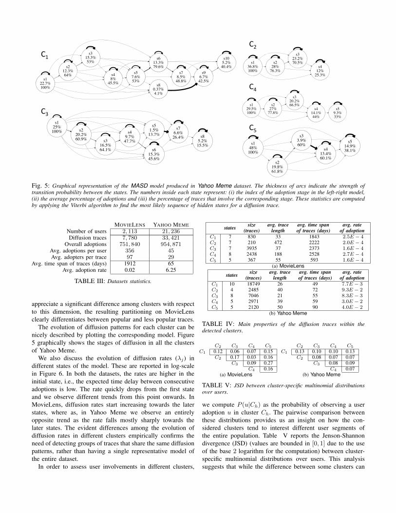
Fig. 5: Graphical representation of the MASD model produced in Yahoo Meme dataset. The thickness of arcs indicate the strength oftransition probability between the states. The numbers inside each state represent: (i) the index of the adoption stage in the left-right model,(ii) the average percentage of adoptions and (iii) the percentage of traces that involve the corresponding stage. These statistics are computedby applying the Viterbi algorithm to find the most likely sequence of hidden states for a diffusion trace.
MOVIELENS YAHOO MEMENumber of users 2, 113 21, 236Diffusion traces 7, 780 33, 421
Overall adoptions 751, 840 954, 871Avg. adoptions per user 356 45Avg. adopters per trace 97 29
Avg. time span of traces (days) 1912 65Avg. adoption rate 0.02 6.25
TABLE III: Datasets statistics.
appreciate a significant difference among clusters with respectto this dimension, the resulting partitioning on MovieLensclearly differentiates between popular and less popular traces.
The evolution of diffusion patterns for each cluster can benicely described by plotting the corresponding model. Figure5 graphically shows the stages of diffusion in all the clustersof Yahoo Meme.
We also discuss the evolution of diffusion rates (λj) indifferent states of the model. These are reported in log-scalein Figure 6. In both the datasets, the rates are higher in theinitial state, i.e., the expected time delay between consecutiveadoptions is low. The rate quickly drops from the first stateand we observe different trends from this point onwards. InMovieLens, diffusion rates start increasing towards the laterstates, where as, in Yahoo Meme we observe an entirelyopposite trend as the rate falls mostly sharply towards thelater states. The evident differences among the evolution ofdiffusion rates in different clusters empirically confirms theneed of detecting groups of traces that share the same diffusionpatterns, rather than having a single representative model ofthe entire dataset.
In order to assess user involvements in different clusters,
states size(traces)
avg. tracelength
avg. time spanof traces (days)
avg. rateof adoption
C1 7 830 33 1843 2.5E − 4C2 7 210 472 2222 2.0E − 4C3 7 3935 37 2373 1.6E − 4C4 8 2438 188 2528 2.7E − 4C5 5 367 55 593 1.6E − 4
(a) MovieLens
states size(traces)
avg. tracelength
avg. time spanof traces (days)
avg. rateof adoption
C1 10 18749 26 49 7.7E − 3C2 4 2485 40 72 9.3E − 2C3 8 7046 21 55 8.3E − 3C4 5 2971 39 59 3.0E − 2C5 5 2120 50 90 4.0E − 2
(b) Yahoo Meme
TABLE IV: Main properties of the diffusion traces within thedetected clusters.
C2 C3 C4 C5
C1 0.12 0.06 0.07 0.15C2 0.17 0.03 0.16
C3 0.09 0.27C4 0.16
C2 C3 C4 C5
C1 0.13 0.10 0.10 0.13C2 0.08 0.07 0.07
C3 0.08 0.09C4 0.07
(a) MovieLens (b) Yahoo Meme
TABLE V: JSD between cluster-specific multinomial distributionsover users.
we compute P (u|Ch) as the probability of observing a useradoption u in cluster Ch. The pairwise comparison betweenthese distributions provides us an insight on how the con-sidered clusters tend to interest different user segments ofthe entire population. Table V reports the Jenson-Shannondivergence (JSD) (values are bounded in [0, 1] due to the useof the base 2 logarithm for the computation) between cluster-specific multinomial distributions over users. This analysissuggests that while the difference between some clusters can

1 2 3 4 5 6 7
1e-02
1e+00
1e+02
State
Rat
e of
ado
ptio
n
1 2 3 4 5 6 7
0.01
0.05
0.50
5.00
State
Rat
e of
ado
ptio
n
1 2 3 4 5 6 7
1e-02
1e+00
1e+02
State
Rat
e of
ado
ptio
n
2 4 6 80.01
0.05
0.20
1.00
State
Rat
e of
ado
ptio
n
1 2 3 4 5
0.01
0.05
0.20
0.50
State
Rat
e of
ado
ptio
n
2 4 6 8 10
0.001
0.005
0.050
0.500
State
Rat
e of
ado
ptio
n
1 2 3 4
0.001
0.005
0.0200.050
State
Rat
e of
ado
ptio
n
1 2 3 4 5 6 7 80.001
0.010
0.100
1.000
State
Rat
e of
ado
ptio
n
1 2 3 4 5
0.001
0.005
0.020
0.100
State
Rat
e of
ado
ptio
n
1 2 3 4 5
0.001
0.005
0.020
State
Rat
e of
ado
ptio
n
Fig. 6: Different diffusion rates (log-scale) in the five clusters in MovieLens (top) and Yahoo Meme (bottom).
0 500 1000 1500 2000
0.2
0.4
0.6
0.8
1.0
Time (in days)
Frac
tion
of a
dopt
ions
The Adventures of Huck FinnL'homme qui aimait les femmesKiller MovieTuristasBrain Damage
0 200 400 600 800 1000
0.0
0.2
0.4
0.6
0.8
1.0
Time (in days)
Frac
tion
of a
dopt
ions
Se, jieInto the WildCarsThe Da Vinci CodeLast King of Scotland
0 500 1500 25000.0
0.2
0.4
0.6
0.8
1.0
Time (in days)
Frac
tion
of a
dopt
ions
The Cowboy WayThe portrait of a LadyFairy Tale: A true storyLove is the DevilEarth: Final Conflict
0 1000 2000 3000 40000.0
0.2
0.4
0.6
0.8
1.0
Time (in days)Fr
actio
n of
ado
ptio
ns
Basic InstinctCon AirFlubberChicken RunHarvey Girls
0 200 400 6000.0
0.2
0.4
0.6
0.8
1.0
Time (in days)
Frac
tion
of a
dopt
ions
Away from HerCharlie BartlettWristcuttersSon of RambowThe TV Set
1 10 100 1000 10000
0.2
0.4
0.6
0.8
1.0
Time (in minutes)
Frac
tion
of a
dopt
ions
12345
1 100 10000
0.2
0.4
0.6
0.8
1.0
Time (in minutes)
Frac
tion
of a
dopt
ions
12345
1 10 100 1000 10000
0.2
0.4
0.6
0.8
1.0
Time (in minutes)
Frac
tion
of a
dopt
ions
12345
1 10 100 1000 10000
0.2
0.4
0.6
0.8
1.0
Time (in minutes)
Frac
tion
of a
dopt
ions
12345
1 100 100000.0
0.2
0.4
0.6
0.8
1.0
Time (in minutes)Fr
actio
n of
ado
ptio
ns
12345
Fig. 7: Adoption patterns, in the 5 clusters, MovieLens (top) and Yahoo Meme (bottom).
be explained at user level, other clusters tend to involve thesame users but with different temporal dynamics.
We also look at the differences among the diffusion patternsof different clusters at the level of individual traces. For this,first, we select a few representative traces in each cluster.These traces are the top-5 w.r.t. minimizing the perplexity forthe considered model. Formally:
perplexity(Di|Θh) = exp
{− logP (Di|Θh)
|Di|
}, (4)
where, the numerator is the log likelihood of the adoptiontrace given the model and denominator is the length of thetrace (number of adoptions). Then, for each cluster we plot inFigure 7 the fraction of adoptions with respect to time for thetop-5 representative traces. These plots show homogeneouspatterns of diffusions for the traces belonging to the samecluster; for instance, the second cluster in MovieLens contains
movies that are diffused slowly in the beginning, however,their popularity increases sharply after a certain point.
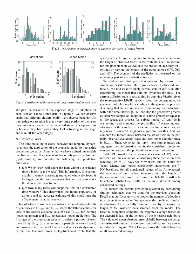
Finally, we study to how many stages a user is associ-ated. We compute user-specific distributions in each stageby exploiting the output of the Viterbi algorithm. We defineP (S(u) = j) as the probability that for a given user, anadoption happens in the j-th stage of the diffusion process, andwe associate the user to a stage only if P (S(u) = j) ≥ 0.1. InFigure 9 we plot the distribution of the number of stages thateach user is associated to. On both the datasets, the figuressuggest that the majority of the users are associated to 1, ormaximum 2, stages of diffusion.
Furthermore, we compute for each user u the expected stagein which we observe his adoption, as:
E [S(u)] =
K∑
j=1
j · P (S(u) = j).
Expected State
Den
sity
of u
sers
in a
sta
te
2 4 6 8 10
0.0
0.1
0.2
0.3
0.4
Expected State
Den
sity
of u
sers
in a
sta
te
1.0 1.5 2.0 2.5 3.0 3.5 4.0
0.0
0.5
1.0
1.5
Expected State
Den
sity
of u
sers
in a
sta
te
1 2 3 4 5 6 7 8
0.00
0.10
0.20
0.30
Expected State
Den
sity
of u
sers
in a
sta
te
1 2 3 4 5
0.0
0.1
0.2
0.3
0.4
0.5
0.6
Expected State
Den
sity
of u
sers
in a
sta
te
1 2 3 4 5
0.0
0.2
0.4
0.6
Fig. 8: Distribution of expected stage of adoption for users in Yahoo Meme.
MovieLens Yahoo Meme
1 2 3 4# of states
% o
f use
rs0
2040
6080 C1
C2C3C4C5
1 2 3 4 5# of states
% o
f use
rs0
1020
3040
50 C1C2C3C4C5
Fig. 9: Distribution of the number of stages associated to each user.
We plot the densities of the expected stage of adoption foreach user on Yahoo Meme data in Figure 8. We can observeagain that different clusters exhibit very diverse behavior. Aninteresting observation is that a very large portion of the usershave an integer value for the expected stage of adoption: thisis because they have probability 1 of activating in one stageand 0 in all the other stages.
D. Predictive tasks
The joint modeling of users’ behavior and temporal dynam-ics allows the application of the proposed model to interestingprediction scenarios. Assume that we have trained our modelson observed data. For a new item that is only partially observed(up-to time t), we consider the following two predictionquestions:• Q1: Which users will adopt the item within a considered
time window (e.g 1 week)? This information, if accurate,enables dynamic marketing strategies where the focus isto target specific user segments that are likely to adoptthe item in the near future.
• Q2: How many users will adopt the item in a consideredtime window? This determines the future popularity ofan item and an accurate estimate of this could tune theeffectiveness of advertisement.
In order to perform these evaluations we randomly split dif-fusion traces in Dtrain and Dtest, where the latter accounts for20% of the overall available data. We use Dtrain for learningmodel parameters and Dtest to evaluate model predictions. Thefirst step of the prediction tasks is to select a portion of eachtrace Di ∈ Dtest (that represents a partially observed trace)and associate it to a model that better describes its dynamics,or, the one that maximizes its log-likelihood. Note that the
quality of the fitting is expected to change when we increasethe length of observed traces in the evaluation set. To accountfor this phenomenon we evaluate the prediction accuracy on 3settings by varying the lengths of the traces among 60%, 50%and 40%. The accuracy of the prediction is measured on theremaining part of the evaluation traces.
We address our first prediction question by means of asimulation-based method. Here, given a trace Di observed untiltime ta, we find its most likely current state of diffusion afterdetermining the model that suits its dynamics the most. Thecurrent diffusion state is easy to find by applying Viterbi (giventhe representative MASD model). From the current state, wegenerate multiple samples according to the generative process.Assuming that we are interested in predicting user adoptionswithin the time interval [ta, tb], we stop the generative processas soon we sample an adoption at a time greater or equal totb. We repeat this process for a fixed number of runs (1k inour setting) and compute the probability of observing useradoptions in the simulated traces. As baseline competitor, werely upon a k-nearest neighbors algorithm. For this, first, wecompute the Jaccard index between the set of users in the par-tially observed evaluation trace and each other adoption tracein Dtrain. Then, we select the top-k most similar traces andaggregate their information within the considered predictionwindow to compute the probabilities of users’ adoptions.
Table VI provides the area-under-the-curve (AUC) valuesrecorded on this evaluation, considering three prediction timewindows, up to 30 days for MovieLens and 24 hours forYahoo Meme. Our model consistently outperforms the k-NN baselines, for all considered values of k. As expected,the accuracy of our method increases with the length ofthe evaluation trace used for fitting, but MASD is still ableto achieve satisfactory results on the most difficult amongconsidered settings.
We address the second prediction question by consideringsimilar techniques that we used for the previous question.Recall that our focus now is to predict the number of adoptionsin a given time window. We generate the predicted numberof adoptions for a partially observed trace by averaging thelength of the synthetic data sampled from the model. Thebaseline competitor computes the weighted average (based onthe Jaccard index) of the lengths of the k-nearest neighbors.The values of mean absolute error (MAE) between the actualand estimated number of adoptions on both dataset are shownin Table VII. Again, MASD outperforms the k-NN baselinein all considered settings.

60% partial observation 50% partial observation 40% partial observationTime Window MASD k-NN (60, 80, 100) MASD k-NN (60, 80, 100) MASD k-NN (60, 80, 100)
30 days 0.70 0.54 0.55 0.55 0.69 0.55 0.55 0.55 0.69 0.54 0.54 0.5521 days 0.69 0.55 0.55 0.55 0.69 0.54 0.54 0.55 0.68 0.54 0.54 0.5414 days 0.69 0.54 0.54 0.54 0.69 0.54 0.54 0.55 0.69 0.53 0.54 0.54
(a) Movielens60% partial observation 50% partial observation 40% partial observation
Time Window MASD k-NN (60, 80, 100) MASD k-NN (60, 80, 100) MASD k-NN (60, 80, 100)60 min. 0.83 0.73 0.74 0.75 0.82 0.72 0.73 0.74 0.82 0.72 0.74 0.7430 min. 0.82 0.72 0.73 0.74 0.81 0.71 0.72 0.72 0.81 0.71 0.72 0.7315 min. 0.81 0.68 0.70 0.70 0.80 0.69 0.70 0.71 0.81 0.66 0.68 0.69
(b) Yahoo Meme
TABLE VI: Area under the curve (AUC) for predicting single user activations in different time windows. The baseline procedure is evaluatedfor three selections of k and three different splits of propagations.
60% partial observation 50% partial observation 40% partial observationTime Window MASD k-NN (60, 80, 100) MASD k-NN (60, 80, 100) MASD k-NN (60, 80, 100)
30 days 3.42 3.90 3.90 3.92 3.71 3.90 3.91 3.92 4.61 5.14 5.17 5.1721 days 2.61 3.02 3.02 3.03 2.88 3.02 3.03 3.03 3.61 3.96 3.97 3.9814 days 1.93 2.22 2.23 2.23 2.16 2.23 2.23 2.23 2.69 2.90 2.91 2.91
(a) Movielens60% partial observation 50% partial observation 40% partial observation
Time Window MASD k-NN (60, 80, 100) MASD k-NN (60, 80, 100) MASD k-NN (60, 80, 100)60 min. 3.57 5.56 5.61 5.63 5.32 7.20 7.24 7.25 7.46 9.01 9.08 9.0930 min. 3.01 4.65 4.69 4.71 4.66 6.13 6.17 6.15 6.69 7.82 7.89 7.9315 min. 2.49 3.23 3.25 3.26 4.53 5.89 5.92 5.93 5.50 5.63 5.66 5.68
(b) Yahoo Meme
TABLE VII: Mean absolute error (MAE) for predicting aggregate user activations in different time windows. The baseline procedure isevaluated for three selections of k and three different splits of propagations.
VI. CONCLUSIONS
In this paper we introduce MASD, a stochastic frameworkfor modeling users’ adoptions and the different stages ofdiffusion of innovations. In continuity with Roger’s theory, ourmodel focuses on the two main dimensions that can explainthe spread of new items through a population, namely the usersand their propensity to adopt a new item in a specific stageof diffusion, and the speed at which adoptions happen in thevarious stages. To capture the evolution dynamics betweenstages of adoptions MASD relies on a left-to-right hiddenMarkov model. The proposed learning procedure allows us todetect fine-grained patterns in the underlying diffusion process.The experimental evaluation over real-world data confirms theaccuracy of the learning framework and its ability to detectdistinct, and interesting, patterns of adoption.
For future work, we plan to investigate an extension ofthe proposed model to account for social influence dynamics.In this scenario, the likelihood of adoption for each user isnaturally expected to increase as more of his social peers adoptthe item. Moreover, each stage of adoption could be furthercharacterized in terms of virality, hence enabling the detection,characterization and prediction of stages in which the adoptionof a product will become viral.
Repeatability. All software (sources and executables) and thesample from Movielens used in our experiments are availableat https://github.com/yasirm/ICDM2014.
Acknowledgments. This work was partially supported byMULTISENSOR project, funded by the European Commis-sion, under the contract number FP7-610411.
REFERENCES
[1] R. Bakis. Continuous speech recognition via centisecond acoustic states.Acoustical Society of America Journal, 59:97, 1976.
[2] E. Bakshy, I. Rosenn, C. Marlow, and L. Adamic. The role of socialnetworks in information diffusion. In WWW, 2012.
[3] C. M. Bishop et al. Pattern recognition and machine learning, volume 1.springer New York, 2006.
[4] C. Budak, D. Agrawal, and A. El Abbadi. Diffusion of information insocial networks: Is it all local? In ICDM, 2012.
[5] A. P. Dempster, N. M. Laird, and D. B. Rubin. Maximum Likelihoodfrom Incomplete Data via the EM Algorithm. Journal of the RoyalStatistical Society. Series B (Methodological), 39:1–38, 1977.
[6] S. Goorha and L. Ungar. Discovery of significant emerging trends. InKDD, 2010.
[7] J. Kleinberg. Bursty and hierarchical structure in streams. Data Miningand Knowledge Discovery, 7(4):373–397, 2003.
[8] J. Leskovec, L. Backstrom, and J. Kleinberg. Meme-tracking and thedynamics of the news cycle. In KDD, 2009.
[9] M. Mathioudakis and N. Koudas. Twittermonitor: trend detection overthe twitter stream. In SIGMOD, 2010.
[10] I. Mele, F. Bonchi, and A. Gionis. The early-adopter graph and itsapplication to web-page recommendation. In CIKM, 2012.
[11] E. M. Rogers. Diffusion of innovations. Free Press, 5th edition, 2003.[12] D. M. Romero, B. Meeder, and J. Kleinberg. Differences in the mechan-
ics of information diffusion across topics: idioms, political hashtags, andcomplex contagion on twitter. In WWW, 2011.
[13] D. Saez-Trumper, G. Comarela, V. Almeida, R. Baeza-Yates, andF. Benevenuto. Finding trendsetters in information networks. In KDD,2012.
[14] G. Schwarz. Estimating the dimension of a model. The Annals ofStatistics, 6:461–464, 1978.
[15] J. Yang and J. Leskovec. Patterns of temporal variation in online media.In WSDM, 2011.