MODELING A REGIONAL ECONOMY II Introduction to SIMLAB An

This document is made available electronically by the Minnesota Legislative Reference Library as part of an ongoing digital archiving project. http://www.leg.state.mn.us/lrl/lrl.asp

MODELING A REGIONAL ECONOMY

An Introduction to SIMLAB II

December, 1977

MODELING A REGIONAL ECONOMY--_•.._----------~._--~,_ .._--~--

An Introduction to SI~rrAB II

By

Donald Newell

Socioeconomic Report DElMinnesota Environmental Quality Board

Regional Copper-Nickel Project

December, 1977

TABLE OF CONTENTS

1. INTRODUCTI ON

A. Purpose of ReportB. The Role of SIMLAB II in Impact AnalysisC. Report Outline

II. REGIONAL FORECASTING

A. Geographic AreasB. Reasons for Regional Socioeconomic ForecastingC. Economic Development Tradeoffs

III. SIMULATION

A. OverviewB. Simulation in Economic Analysis

IV. SIMLAB I I

A. Modular ApproachB. Regional Input-Output Transaction Table DevelopmentC. Introduction to SIMLAB II Modules

1. Production moduleI '2. Market modul e

3. Demand module4. Investment module5. Population module6. Labor force module7. Employment module8. Value added module9. Household module

V. LOADING SIMLAB II

A. Data Base RequirementsB. Basel ine ForecastsC. Val i dation of Basel ine ForecastsD. Alternative Futures Forecasts

VI. SUMMARY AND CONCLUSIONS

MODELING A REGIONAL ECONOMY

INTRODUCTION

Purpose of Report

This report introduces the forecasting techniques used by the Minnesota

Environmental Quality Board's Regional Copper-Nickel Study to explore the

economic and demographic impacts of alternative futures reflecting varying

degrees of copper-nickel mining development in northeastern Minnesota.

The forecasting model used was developed by Dr. Wilbur Maki, Professor,

Department of Agricultural and Applied Economics, University of Minnesota,

and is called SIMLAB II (Simulation Laboratory II). SIMLAB II is presently

operational for two multicounty regions plus the state as a whole. Future

development plans include the modeling of each of Minnesota's thirteen

development regions (Figure 1). Once modeled, the system will be made

available to state planning agencies and the respective regional development

commissions.

The Role of SIMLAB II in Impact Ana~

The role of SIMLAB II in the Regional Copper-Nickel Study is somewhat

mechanical. The outcome of a particular forecast depends on the assumptions

used in making that forecast. For example, the "baseline" forecast,

against which we measure impacts, rests on the assumption that the historical

relationship between the regional economy and the national economy continues.

(For example, the relationship between a regional sector's gross output and

the national sectors· gross output.) It is the task of the study team to

develop realistic and/or potential changes in this relationship which would

I,

(As of Sept. 30, 1974).

Winona

REGIONAL DEVELOPMENTCOMMISSION NAME

1 Northwest2 Headwaters3 Arrowhead4 West Central5 Region Five6E Six East

·6W Si x West7E East Central7W Central Minnesota8 Southwest9 Region Nine10 Southeastern11 Metropolitan Council

7E'

Mower

Pine

Kanabec

Crow 'YJ,ng

5

Itasca

Morrison

Meaker

G'E

'Todd

,,"Va dena

,

-----r~Slearn. 7

ls

1

ChIPP~-

L l"coln Lyo.,

Cia)' Becker

Norma,..

Figure 1.

II

Page 2

alter the baseline conditions. This is referred to as developing alternative

futures for the region. One could hypothesize the eventual decline in

regional taconite mining and see how this would effect the region's economy.

In addition, the study team must develop alternative copper-nickel mining

scenarios to assess the impacts of such development. From a policy-making

standpoint the important consideration is the ability to overlay these

scenarios on the different alternative future forecasts to assess the

impacts of copper-nickel mining under varying economic conditions. For

example, a staged copper-nickel mining development of a particular scale

would help offset the decline in employment resulting from taconite mining

curtailment, resulting in a more stable employed work force. It is the

study team's task to develop the assumptions and alternatives; SIMLAB II's

role is to process them. One of the final reports generated by the study

will develop this impact analysis.

Report Outline

Section one identifies the Regional Copper-Nickel Study area and the potential

uses of regional forecasts. Section two will focus attention on the concepts

and uses of simulation techniques in general, and its applicability to

socioeconomic systems in particular. Section three discusses the modular

approach to simulation model design, and an introduction to each SIMLAB II

module. Section four identifies SIMLAB II data requirements, potential data

sources, and explains procedures used in forecasting alternative development

scenarios. Section five contains a summary and discusses future research

potentials.

Ii

Page 3

REGIONAL FORECASTING

Geographic Areas

In the past state agencies have often been accused of allowing local or

regional socioeconomic impacts to be overshadowed by the larger state-wide

impacts when considering policy alternatives. From the agency point of

view this is understandable, and in many instances justifiable. This is

not the case in the present study. The Copper-Nickel Study has the task

of developing a regional socioeconomic impact analysis capability to

assess the potential impacts associated with proposed copper-nickel mining

activity in northeastern Minnesota.

Two geographic areas have been identified for detailed analysis (Figure 2).

The pr-imary impact area, called "The Regional Copper-Nickel Study Area"

(RCNSA), covers 2000 square miles and includes the following eight commu-

nities as areas of major emphasis:

1) Aurora2) Babbitt3) Biwabik4) Ely5) Eve1eth6) Gi 1bert7) Hoyt La kes8) Virginia

Reasons for Regional Socioeconomic Forecasting

The primary rationale for selecting this area was the fact that Virginia

and Ely are the two major East Range marketing areas, and the expectation

that most settlement by construction employees and operations workers would

occur in this area. Thus, the study area is bounded by the two communities.

E

\

:"-.··_···,..·· .....~~JD

. ARTAGE5J,KooC

~©~~\>

~1!},~~

./... ""':/ ..( L.., CA ADA.// l \....__........c. ... - .. '- .._ ...-"'-.

I N

iiil---.---------IIII _._ .. _

~.-.---L-----l WISCONSIN

i p II 'I i COUGLAS, '

• I I'I' :__._. .J 1---" -"---"-"-"

T A 13 C A

r ,--..._, Figure 2 , 1

I! l_.i -_._.-..._\ :~i~·;~·~~~f-;f.1.~~/)4, :) FALLS -"-"j ' ..._ ...-""-'" I' "I :- ..

I' _ ...· ,I ~· I I! i:I '\.i ! \ .! I<OOCHICHING I .>I , ...., II .· II '· \J II '! ~: I~------~---_._- --------_._-------~ .;

! I!!ii~' . ~-........I - '/

The secondary impact area is composed of Minnesota Economic Development

Region III (Arrowhead) plus Douglas County in Wisconsin. This delineation

was selected because the Copper-Nickel Study area falls within Region III,

and Duluth, Minnesota is the major service center of the Arrowhead Region.

Douglas County, Wisconsin, was included because of the importance of

Superior, Wisconsin's port facilities and the possibility of siting a

copper-nickel smelter in Douglas County.

Development of Minnesota's copper-nickel are resources may significantly

alter the economics of several northeastern communities. The massive

influx of capital would create hundreds of new jobs. Initially, construction

activity would attract many temporary migrants which could create a potential

housing shortage. Eventually, these temporary workers would be replaced by

permanent mining employees who have different housing needs and preferences

as indicated by a study 0 f coal mining development in North Dakota

(Wiel~nd, 1977). Construction and mining development payrolls would

increase demand for locally produced goods and services. Such increases

would provide additional business and employment opportunities. Concomitant

demand for increased public services could severely strain existing facilities

and capacities. Clearly, a systematic assessment of these and other socio

economic impacts is prudent and necessary.

Economic Development Tradeoffs

When state agencies are considering questions concerning economic growth

and development, the tradeoffs associated with different development

strategies should be a parameter examined prior to making decisions

significantly affecting such growth and development. Faced with limited

I,

Page 5

capital budgets, some desirable projects must be delayed or rejected.

Thus, the impacts associated with a particular project should be compared

to the impacts generated by other projects. Projections of project

benefits like employment or regional income should be made to ensure that

the agency is getting a "maximum" return on its spending. If, for example,

the state was dedicated to increasing the well-being of a particular region,

and had the option of promoting either a new forest products industry or

building a new state park, the effects of each decision could be measured

·and compared. SIMLAB II was developed for this purpose. Namely, to

assist decision-makers in their policy deliberations.

SIMLAB II has been selected by the Copper-Nickel Study group as the ana

lytical tool needed to make such assessments. In order to isolate the

various effects mining development would have on the impacted study area,

IIbaseline ll forecasts of relevant socioeconomic indicators must be made.

Baseline forecasts are merely projections produced by the model in the

absence of copper-nickel mining development. Phased construction and

mining development scenarios are then introduced and the results are

compared with the baseline forecasts to calculate the resultant impacts.

Thus, the user can postulate an almost unlimited number of changes and

isolate their impacts.

SIMULATION

Overview

Simulation makes possible predictions of how a system may behave in cases

where experimentation on the system under study would be impossible. For

example, the consequences of proposed economic development on a regional

.'

Page 6

economy. Thus, to simulate is to dup"licate the essence of the system or

activity without actually attaining reality. Simulation itself is an

approximat-ion of reality, and the intent of simulation research is to

reveal something about that reality. In the present case, what is needed

is a systematic approach to identify and analyze those demographic and

economic characteristics relevant to the study of a regional economy. A

simulation consists of writing down, or otherwise agreeing upon, a set of

realistic assertions. The realism of these assertions is established

outside the simulating system itself (e.g. by actual observation or

experience). The investigator then constructs a system which describes

the simulation in mathematical terms (e.g. a mathematical model or computer

program), and tests whether or not the system can predict the realistic

assertions within the required degree of accuracy.

The term "simulation" is commonly used in business, econom-jcs, and other• • I' .,

soci~l sciences to refer to the operation of a numerical model that

represents the structure of a dynamic process. Given initial values for

the model parameters (variables which are specified in the model), a

simulation is run to represent the behavior of the system over time. Thus,

a simulation run is considered to be an experiment on the model, with the

initial set of variables describing the state of the system at the

beginning point in time. The results of the simulation are the values of

the variables at the end of the time interval. The time period simulated

can vary from one to several time periods (e.g. from one to twenty years)

with the model using the results of preceding time periods as input values

for successive time periods. This process is sometimes referred to as

"recursive iteration," or "recurrence modeling."

There has been an increasing awareness that business and economic problems

must be looked at in terms of the total economy with all the attendant

interactions between the parts, and simulation offers an excellent tool

for analytical purposes. Decisions and policies must be evaluated on the

basis of their impact on the immediate behavior of the economy and their

long run consequences on more remote parts of the economy. Thus, it is

necessary to consider not only the actions in one part of the economic

system, but also reactions of other components in the system.

Simulation in Economic Analysis

Economists have long sought ways of modeling the dynamic behavior of

economic systems over time. Simulation is an ideal tool for long-range

economic analysis. It not only allows the analyst the ability to determine

the long-run state of the system, but also to analyze the time path through

which the system travels to reach the final state. Economists have found

it useful to distinguish between macro models (which deal with whole systems)

and micro models (which deal with the behavior of individual units).

Typical macro models include those which employ large econometric models

of the U.S. economy, usually designed to forecase aggregate, or total

Gross National Product (GNP). Alternatively, micro models attempt to

forecast the gross output of various industrial sectors and then aggregate

them to derive total GNP. This approach has been justified by the following:

Predictions about aggregates are needed, but they should beobtained by aggregating behavior of elemental units ratherthan by attempting to aggregate behavioral relationships ofthese elemental units. That is, aggregates should be obtainedfrom a simulation of the real system in a fashion analogousto the way a census or survey obtains aggregates relating toreal socioeconomic systems. Given a satisfactory simulation

of the socioeconomic system developed in terms of the elemental decision-making units, aggregation of relationshipsVJould become more nearly feasib"le. Such aggregat"ion would beinteresting and useful, but it would no longer be a necessity(Oncutt, 1961).

This process, of course, is the expressed fort~ of SIMLAB II.

SIMLAB II has been referred to as a simulation model. A model is simply

a constructed expression of a theory or hypothesis. By constructed we

mean they do not appear naturally, rather, they are the creation of man.

For example, the model airplane 'Iflown ll in a wind tunnel is an expression

of the theory of flight. A model of the behavior of a firm is, likewise,

an expression of the economic theory of the firm. Simulation models are

just a special subset of models. They exhibit certain properties in

addition to all the characteristics of general models. A simulation model

has the following properties:

1) rf is intended to represent all or part of a system.

2) It can be executed or manipulated.

3) Time or a count of repetitions is one of the variables (i.e. thesystem is simulated over time).

4) Its purpose is to aid understanding of the system being simulatedwhich means one or more of the following:

a) it is a description of the systemb) its use attempts to explain past behavior of the systemc) its use attempts to predict future behavior of the systemd) its use attempts to teach the existing theory by which the

system can be understood.

As stated earlier, the purpose of economic simulation models is to aid in

our understanding of the economy in which we are interested. Understanding

means we can identify the important inter-relationships within the economy,

and determine how variables in the economy react to changes. The ultimate

test of understanding is our ability to predict future behav'ior of the

system. If we can accurately predict its behavior, we may then be in a

position to control or influence the economy to meet some predetermined

set of goals. Thus, the purpose of using a simulation model such as

SIMLAB II for socioeconomic forecasting of a regional economy is to aid in

our understanding of the region and to aid in the development of regional

policies.

There are several terms which are used by analysts w~o build and use

simulation models. First, we define a II run ll of the simulation as cycling

through the operations of the model for a measureable'amount of time.

Next we define a IIparameterll of the model as a number or symbol that

remains constant during a run of the simulation (e.g. the fertility rate

by age). Parameters are often called "variable constants,1I since they can

be changed from run to run. Parameters are normally input constants.

That'is, they are specified by the user at the beginning of the simulation

run.

Finally, we define a II var iable ll as an entity which can take on different

values during a single simulation run. Two types of variables are used in

simulation models. Input variables (which are often called exogeneous

variables) are external to the model (e.g. the regional market share of an

industry). That is, they must be changed by the user. Generated variables

(endogeneous), on the other hand, take on values which arise as a conse

quence of the operations of the model (e.g. total population). These

generated variables are usually the most interesting to analysts or users.

Once the operations, parameters, and input variables are specified,

experimentations with the model can take place. This usually consists of

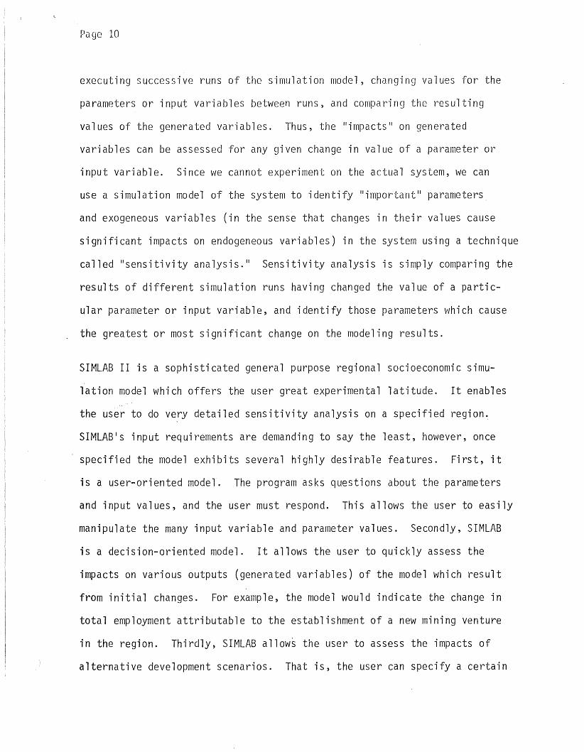
executing successive runs of the simulation model, changing values for the

parameters or input variables between runs, and comparing the resulting

values of the generated variables. Thus, the "impacts" on generated

variables can be assessed for any given change in value of a parameter or

input variable. Since we cannot experiment on the actual system, we can

use a simulation model of the system to identify "important" parameters

and exogeneous variables (in the sense that changes in their values cause

significant impacts on endogeneous variables) in the system using a technique

called "sensitivity analysis. 11 Sensitivity analysis is simply comparing the

results of different simulation runs having changed the value of a partic

ular parameter or input variable, and identify those parameters which cause

the greatest or most significant change on the modeling results.

SIMLAB II is a sophisticated general purpose regional socioeconomic simu

lation model which offers the user great experimental latitude. It enables

the USer to do very detailed sensitivity analysis on a specified region~

SIMLAB's input requirements are demanding to say the least, however, once

specified the model exhibits several highly desirable features. First, it

is a user-oriented model. The program asks questions about the parameters

and input values, and the user must respond. This allows the user to easily

manipulate the many input variable and parameter values. Secondly, SIMLAB

is a decision-oriented model. It allows the user to quickly assess the

impacts on various outputs (generated variables) of the model which result

from initial changes. For example, the model would indicate the change in

total employment attributable to the establishment of a new mining venture

in the region. Thirdly, SIMLAB allow~ the user to assess the impacts of

alternative development scenarios. That is, the user can specify a certain

development scenario (e.g. phased construction and operation of the new

mining venture), then manipulate the timing or intensity of the development

and compare the total impacts. Clearly, SIMLAB II is a very flexible,

versatile tool for socioeconomic impact forecasting.

SIMLAB II

Modular Approach

An essential ingredient of a practical and successful simulation model is

a clear and precise focus on purpose. Since SIMLAB II is a general purpose

simulation model it must be adapted or modified in such a way as to make

it issue specific. In the present case the express purpose of the study is

to identify and analyze the economic and demographic impacts of alternative

copper-nickel development strategies in northeastern Minnesota. This

purpose is noted here because much of the following discussion will relate

or refer directly to this research effort. Any decision, when implemented,

impinges upon and changes the future state of reality from what it would

be if alternative actions had taken place. Truth, in decision making, lies

in the future and is beyond the grasp of present perception. Thus, the

perceived outcome of present actions is a function of the confidence one

has in the simulation model employed in predicting future behavior of the

system. For many systems confidence is high, while in others confidence is

lower. This is directly related to our understanding of the system under

consideration. When systems are complex, which is the case in a study of

regional socioeconomic activity, it is often more prudent to subdivide the

system into several inter-related components. This, in effect, simplifies

the modeling procedure by enabling the analyst to isolate sections of the

system and building separate models for each section. To complete the

model the analyst must then specify how the subsections "fit" together

and develop a control module to manipulate the model as a whole. In

essence, the control module "directs" the flow of information within the

mo del . That is, i t 1inks th e different sec to rs toeachother when the

output or result from one sector is an input or requirement of another

sector. For example, the labor force module in SIMLAB II requires as an

input the age/sex population distribution from the population module.

Similarly, the employment module requires information from both the

production module and the labor force module. While each module stands

alone in the sense that it is internally consistent with existing theory,

the modules are linked together to form a broader dynamic socioeconomic

model.

SIMLAB II utilizes the control module to execute the simulation model

computer program. As noted above, the control module directs the flow of

information through the simulation. The modular approach was selected

for two reasons: 1) because it facilitates understanding of the model

itself (i.e. it attempts to simplify the total model); and 2) it enables

future development to be easily adopted. For example, a tax module which

analyzes the financing and delivery of local government service could be

readily incorporated into the existing model framework. The remainder of

this section will focus on a discussion of each of the nine modules,

identifying their major data input requirements, how they are linked to

other modules and their relative importance to the total model, and finally

the major assumptions underlying the theory each module attempts to model.

Economic activity is defined as the process of producing and consuming

goods and services. In the absence of human wants (or needs) the concept

of economic activity would be irrelevant. It is precisely this demand by

people which calls forth the production of consumer goods and services.

As will be seen shortly, the production module Iidrives" the socioeconomic

system we are seeking to model, and herein lies the heart of SIMLAB II.

Regional economists have long recognized the role exports play in supporting

the economic activity within a region (Tiebout, 1956). Exports of goods

and services represent sales to consumers outside the region (or tourists

visiting the region). The revenue generated by this export production

enables workers residing in the region to purchase locally produced goods

and services. These purchases in turn provide employment opportunities and

further spending within the region. Thus, the first task is to identify

these various transactions. This is accomplished by utilizing an accounting

framework called Input-Output Analysis (1-0). Development of the framework

is attributed to Nobel Prize Winner, Wassily Leontief (1951). Basically,

Input-Output Analysis (hereafter referred to as Interindustry Transactions)

identifies the purchases and sales of homogeneous sectors within the economy.

These purchases (and hence sales) represent the input structure of the

producing sectors. Economists generally refer to these purchasing patterns

as "production functions. II Production functions represent the input

requirements for an industry enabling that industry to produce its output

products. For example, one important input to the automobile industry is

sheet metal. In the interindustry transaction table (a table that records

purchases and sales between all sectors), this would be represented by a

purchase by the automobile industry from (and hence a sale by) the fabricated

metals industry. Once we have identified all these interindustry purchases

we can b~gin to analyze the impacts on all industries which result from

the expansion of output from any given industry. These impacts are divided

into primary and secondary 'impacts. Primary or direct 'impacts represent

the direct purchases of the producing industry. Secondary or indirect

impacts refer to the increase in output required from industries who supply

inputs to those sectors directly supplying the producing industry. In the

case of an expansion in the automobile industry, increased demand for sheet

metal would represent a direct impact, while increased demand for iron ore

mining (an input for sheet metal producers) represents an indirect impact.

The total impact of increased production is derived by utilizing a

mathematical technique called the "Leontiff Inverse" and is often referred

to as the industry "multiplier. II This multiplier measures the total impact

of expanding the output of any given industry to meet the increased demand

of final users.

Thus, the initial task is to produce, for the region, an interindustry

transaction table which represents the transactions which take place

between firms ~ith1.n the reg-ion. This point -is important since it is only

purchases and sales among firms within the region which give rise to

multiplier effects. Purchases made from outside the region (imports)

represent "leakages" within the economy. That is, it is money which

escapes the local economy.

Regional Input-Output Transaction Table Development

Regional interindustry transaction tables can be constructed from either

primary or secondary data sources. Primary data collection t"epresents a

considerable expenditure of time and money. After identify'ing the sector

classification system to be used (i.e. assigning regional firrns to producing

sectors) a sample of firms from each sector must be contacted. Purchases

and sales data must be collected and analyzed and a sector production

function developed. Because of the sizable costs 'involved in primary

collection, techniques which utilize secondary (or limited primary) data

have been developed which utilize published U.s. transactions data to

derive a regional transaction table (Hwang, 1976). Two critical assumptions

must be adopted when using these techniques. First, we assume that the

purchasing pattern of sector firms within the region are the same as

sector firms in the U.S. as a whole (i.e. their production function is the

same). Secondly, we assume that if an input requirement is produced locally

it will be purchased locally. This assumption rests on the proposition

that the producing industry will buy from the least cost seller, and since

local"producers would have a comparative price advantage (lower transpor

tation costs), the buyer would purchase the input locally.

In addition to the U.S. transaction table we need estimates of total

regional gross output by sector and estimates of final demand (that portion

of output purchased by final users, i.e. households and government). Once

we know the amount of output produced we can derive the level of inputs

necessary to produce that output (from the first assumption above). If

input requirements can be met from local sources they will be satisfied

locally (second assumption). If the gross output of a firm exceeds the

amount required locally the residual is assumed to be exported out of the

region. This distribution of gross output results in the derivation of a

regional interindustry transactions table, which is, of course, the heart

of the production module.

Introduction to SIMLAB II Modules

SIMLAB II, as presently constructed, consists of the following nine

modules:

1) Production2) Market3) Demand4) Investment5) Population6) Labor Force7) Employment8) Value Added9) Household

In addition, the model has the control module discussed above. While each

module can stand apart, it is the interaction between the modules which

produces our regional socioeconomic forecasts. Each of the specified

modules and how they interact will be discussed below.

Production Module--The derived interindustry transact"ion table identifies

the economic linkages which exist between firms within the region. These

linkages, or endogeneous transactions, are assumed to hold over time and

level of output. That is, the purchasing pattern of a given sector remains

constant, and an increase (or decrease) in output production results in a

corresponding proportional increase (or decrease) in purchases from all

other sectors (referred to as a "linear" production). While this "static"

nature of the economic system has been criticized it remains tenable at

least in the short run. The user, however, does have an option. In

light of superior information, he can adjust the production function in the

original transaction table and produce a new set of relationships. This

is representative of the strength of SIMLAB II. That is, the ability to

,quicklY and easily modify the program parameters or variables.

Once these technical relationships have been specified the production

module is linked to national markets via the market module (see following

discussion) which calculates the "reg ional market share" of each sector,

which represents the sectors' share of U.S. production. In addition, a

percentage change in regional market share is calculated using historical

time series data and trend analysis. Together, these translate into

future regional industry exports when linked to independent projections

of U.S. gross output by sector. Thus, there is a critical link established

between the regional economy and the national economy as a whole. The

remaining components of final demand (see following discussion) or demand

for locally produced outputs are internally derived and taken as a whole,

"drive"the production module.

There are, however, constraints within the model which could prevent the

attainment of demanded gross output. First, there is an output-increasing

capacity limit. If gross output demanded exceeds the region's ability to

produce because of insufficient plant and equipment investment in new

capital must be undertaken. The production module, however, recognizes

that there is a limit on the amount of new plant capacity which can be

installed in a given time period. In addition, environmental constraints

require some industries to include investment in pollution abatement

equipment which also limits the amount of new output-capacity expansion

which can be undertaken. The third and final production constraint

recognizes the potential absence of skilled labor inputs. If the resident

labor force is insufficient to meet industry labor requirements, and this

deficiency cannot be overcome through in-commuting, gross output demanded

will not be realized. The relevant output of the production module is,

therefore, realized gross output by industrial sector.

Market t19-iJQJ~--In an open economy (where trade is an important proportion

of total economic activity) the viability of a region is heavily dependent

upon its export base. Regions, however delineated, inside the u.s. are

considered open economies and must, therefore, engage in trade in order to

survive. The money generated by regional export sales goes to pay for

imports of raw materials or semifinished goods. Wages paid to employees

in the export industries enable local households to purchase goods and

services produced locally (as well as imports of finished goods). The

market module is used to link the reg-jonal economy to the national economy

by comparing regional production by industrial sector to national production

by that sector. This comparison yields a "reg -jonal market share" for each

regional industry. Together with an estimate of how that market share

changes over time (i.e. annual percentage change in regional market share),

and independent projections of U.S. gross output by sector, demand (by the

rest ~f the nation) for regional production can be derived. This derived

demand by sector represents the projected export column in the table of final

demands. This table is the subject of the next module.

Demand Mo~ule--Producers of goods and services in a competitive free

market economy respond to the desires of final consumers. Without demand

for its output the firm or industry will not survive.

The demand module provides the entries necessary to complete the final

demand table referred to in the production module. In addition to pro

ducing goods and services for export markets, regional production also

satisfies intra-regional demands of final consumers. Final consumers are

defined here as the final user of the product or service. That is, the

final consumer does not purchase the product for further processing, but

rather represents the end use of a product. Final users are generally

classified as household consumer (or personal consumption expenditures,

PCE), state and local governments, federal government, and business

(private fixed capital formation, PFCF). The business sector contributes

to final demand in two ways. First, a column representing net inventory

change which represents business investment in inventory. These are goods

produced but not yet delivered to one of the other final users. It is the

difference between current production (gross output) and net deliveries

(net sales) for each producing sector. The second business final demand

column represents business investment in new or replacement plant and

equipment, commonly called private capital formation. These entries are

derived in a separate investment module (see following discussion).

Personal consumption expenditures represent purchases by households for

current use. The level of household expenditures depends on a lagged

relationship between consumption in the previous period and personal income

in the present period. The distribution of.purchases to producing indus

tries is accomplished using information on consumer purchases published by

the U.S. Department of Labor and the U.S. Census Bureau. State and local

government expenditures are similarly derived utilizing nationally prepared

distributions of purchase to producing sectors. The level of expenditures

is also based on a lagged relationship between historic per capita expen

ditures and current government revenue (which is based on personal and

business taxes and payments). Another component of final demand is federal

government expenditures. Federal expenditures are considered independent

(or exogeneous) to the regional economy, and the level of regional expendi

tures is based on an estimate of previous per capita federal government

expenditures and annual rates of chanqe in per capita expenditures. Again,

the distribution of purchases to producing industries is based on published

federal sources (i.e. Bureau of Economic Analysis). A much more compre

hensive fiscal (government) module is presently being developed and will

be incorporated into SIMLAB II.

The last component of final demand is the business investment referred to

above. The next section will cover the derivation of this column in more

detail. The result of the foregoing analysis is f-inal demand table. It

represents the sales made by each producing sector to each final user.

This final demand table (or matrix as it is often called) is used in the

production module to determine the gross output demanded from each producing

sector in the regional economy (and coincidentally regional exports and

imports). The reader is reminded here that output demanded need not be

output realized. Constraints within the production module (referred to

elsewhere) are applied to determine the actual (realized) gross output

produced." We now turn our attention to the investment module.

Investment Module--In order for a firm to maintain its productive capacity

it must continually replace worn-out plant and equipment. To increase its

capacity the firm must usually add to existing plant and equipment. This

"investment" in capital (producing) goods is accounted for in the

investment module. As noted above, investment is a component of final

demand and is a column'of transactions which represen sales of capital

goods to business users. There are four types of investment in the

investment module. The first type is replacement capital, and the assumption

a~opted is that firms will purchase enough capital goods to maintain present

capacity. That is, purchases will at least equal current depreciation.

P-aqe 21

In addition, if demand for its output increases firms will attempt to

purchase new plant and equipment for expansion of capacity, which is the

second type of investment. Investment -in pollution abatement capital is

isolated in SIMLAB II and constitutes the third and fourth types of

investment. Again, investm~nt in pollution abatement equipment will be at

least sufficient to maintain present output capacity. If output increasing

capital is purchased a corresponding amount of investment in new pollution

abatement capital is necessary. Capital producing sectors are identified

according to the classification system adopted, and total investment is

allocated to the relevant sectors using a capital requirements matrix and,

as indicated above, represent sales by capital--producing sectors to final

demand.

Population Module--The dynamics of regional population change requires

considerable interaction with the production module. This interaction is

necessary to calculate the migration component of the population module.

Initially, the standard cohort survival technique is employed to calculate

the natural increase in regional population. Thus, population at the

beginning of the time period depends on the previous initial population,

plus births during the interval minus deaths during the interval. Births

are calculated by applying fertility rates developed by the State Demographer.

Deaths are calculated by applying standard actuarial tables to each cohort

(age/sex group). The migration component of the population module is perhaps

the most difficult to forecast. There are many reasons why people move

which cannot effectively be modeled (e.g. to be closer to relatives). Thus,

the assumptions which underlie the migration component are the most tenable.

SIMLAB II assumes that migration is associated with employment opportunities.

If unemployment in the reg-jon exceeds a specified level out~migration wil"1

occur. Alternatively, if unemployment is low, representing a deficiency

in the supply of labor, in-migration will occur.

The upper anel lower unemployment bounds which "trigger" this migration are

subjective and depend on the region under study as well as the national

rate of unemployment. The model user is asked to specify these bounds

prior to the simulation run. This demand for labor services (employment)

is directly tied to demand foY' regional production. Final demand determines

the output level required by each sector. This output level requires labor

inputs which are specified by the industries' occupational profile and

output per worker ratios. These labor requirements, by occupation, are

used by the labor force module which in turn determines the level of

employment (and unemployment). The population module then uses this infor

mation to calculate the migration component of population change. Thus, it

can be seen that considerable interaction between several modules must

occur before population change can be determined.

Labor Force Module--The primary function of the labor force module is to

calculate the available supply of regional labor by occupation class. The

production module can then draw on this labor pool to satisfy its demand

for labor. The initial labor force and occupational structure are iden

tified using existing secondary data (census of population) supplemented

by primary data sources where available. In the Copper-Nickel Study a

comprehensive household survey was conducted. Labor force par·ticipation

rates are calculated for each age/sex cohort. The number of individuals

in the residential labor force are then derived by applying these rates to

the residential population. Since labor force participation rates are

sometimes highly volatile, the model allows easy access to the labor force

module to change these rates when supplemental information suggests

adjustments are necessary. Estimates of out-commuting workers reduce the

available local labor supply while in-commuters add to the pool. Once the

available labor force is identified (by occupation class), it is matched

with the labor demand schedule generated by the production module. If the

supply of a particular occupation class is greater than the demand for that

class, the excess is assigned to an unemployment submodule. If the supply

of an occupation class is insufficient the deficiency is assigned to the

unemployment submodule as a negative entry. This unemployment submodule

is then used to select the occupation of migrants. For example, if the

unemployment rate for a given occupation exceeds a specified level some

members of that occupation class will migrate out of the region. Alterna

tively, if there is an insufficient number of workers in the available

lab~r force (negative entries) this demand will be met during succeeding

time periods through additional in-com~uting and in-migration. Thus, the

overall model allows for adjustments in the occupational profile of the

residential labor force toward some equilibrium (i.e. trigger rates

selected by the user). These values are then utilized by the population

module to determine future population changes.

Employment Module--The employment module links the production module with

the labor force module via an estimate of output per worker for each

producing sector. In addition, an industry profile matrix is used to

estimate the required number of workers by broad occupational categories

for each sector. The occupational requirements of each sector are then

summed and compared with the residential labor pool. If, after allowing

for commuting and limited migrat-ion, the necessary workers are not

available, gross output is constrained (this is the labor constraint

alluded to in the production module). The employment module allows for

reduced labor requirements over time by applying Bureau of Labor Statistics

increases in labor productivity. The occupational profile for each

industry, however, remains constant. Earnings per worker are also calcu

lated by applying the productivity increases to the industry wage bill.

This assumes that wage increases parallel productivity gains. The earnings

per worker calculations are used in the value added module which is used to

distribute business income.

Value Added Module--Value added refers to that portion of the value of a

product which is attributed to the producing (selling) industry. For

example, a bakery will purchase flour and other ingredients to produce

bread, which it then sells to final consumers. The difference between

what'the bakery paid for the necessary inputs and the selling price is

referred to as the II va l ue added. II Raw materials may pass through several

stages of production with each successive stage contributing some value

added. Ultimately, the cost of production inputs (materials) plus the

value added must equal the selling price, which final users must pay. This

value added must then be allocated to various categories which is the

function of the value added module.

The value added module calculates employee compensation (wages, salaries,

and fringe benefits) plus proprietory income (earning of self-employed

persons). Indirect taxes are related to gross output and historical trends

in tax rates. Depreciation of capital, both production and pollution

abatement, is calculated (and used as an input to the investment module).

Business profit is the residual of gross output nlinus employee compensation

minus indirect taxes minus depreciation and minus imports (which are calcu

lated in the production module). Imports being production input requirements

which are not locally available. Total personal income is then adjusted

for governmental transfer payments and income derived from other sources

(e.g. stock dividends) to equal published Bureau of Economic Analysis Regional

Economic Information System Control totals. This total income figure is

then distributed to households in the ninth and final module.

Household Module--Personal consumption expenditures are derived on a house

hold basis, which means it is necessary to allocate regional population to

household formations. Based on census data and primary data sources

(i.e. the Copper-Nickel Study household survey), the number of consumer

units (people) per household are derived by occupation and income class

(which is based on occupation). Personal consumption expenditures are

derived for each household income class and is used in the demand module

as a component of future final demand. Income taxes and indirect taxes

(i.e. sales tax) are also derived with personal savings being the residual.

These outputs will be used in the fiscal module currently being developed.

LOADING SIMLAB II

Data Base Requirements

In order to produce baseline forecasts for a region SIMLAB II must be

IIl oaded" with certain data elements which are specified by the model.

While some SIMLAB parameters are already specified based on national or

state data (e.g. industry capital/output ratios, or age cohort fertility

rates) these may be readily modified by the user where regional conditions

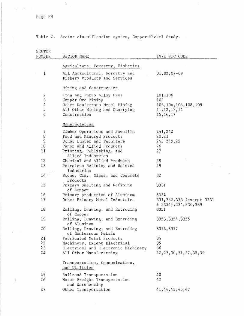
suggest these values are significantly different. Table 1 lists the input

data requirements, and Table 2 lists the Copper-Nickel Study Industrial

Classification System. Once specified, baseline forecasts are made for

the following indicators (by year).

1) Population by age/sex cohort (14 cohorts).2) Residential labor force by age/sex cohort (6 cohorts).3) Employment by industrial sector and occupation.4) Personal income per capita.5) Gross output by industrial sector.6) Value of exports by industrial sector.7) Value added by industr-ial sector.

Table 1. SIMLAB data base.

1) Population, by age (1 to 65 and over) and sex.

2) Migration probability, by age and sex.

3) Death rate, by age and sex.

4) Fertility rate, per 1000 females.

5) Labor force participation rate, by sex and age group.

6) Total unemployment data, by occupation.

7) Total employment, by industry.

8) Total gross output, by industry.

9) Total output per worker, by industry.

10) Rate of change in output per worker, by industry.

11) Total (U.S.) gross output, by industry.

12) Regional market share, by industry.

13) Rate of change in regional market share, by industry.

14) Total (U.S.) growth rate, by industry.

15) Total regional final demand, by industry.

15.1 personal consumption expenditure15.2 gross private capital formation15.3 business inventory change15.4 export (to rest of nation)15.5 state and local government expenditure15.6 federal government expenditure

16) Earnings per worker, by industry.

Table 1. (contd.)

17) Rate of change in earnings per worker, by industry.

18) Income elasticity of demand, by industry.

19) Own-price elasticity of demand, by industry.

20) Output producing capital, by industry.

21) Output-increasing capital-output ratio, by industry.

22) Expansion investment, output-increasing, by industry.

23) Replacement investment, output-producing, by industry.

24) Rate of change in output-increasing capital-output ratio, by industry.

25) Depreciation rate, output-producing capital, by industry.

26) Pollution Abatement capital, by industry.

27) Pollution abatement capital-output ratio, by industry.

28) Expansion investment, pollution abatement, by industry.

29) Replacement investment, pollution abatement, by industry.

30) Rate of change in pollution abatement capital-output ratio, by industry.

31) Depreciation rate, pollution abatement capital, by industry.

32) Total primary input, by industry.

32.1 employee compensation,,32.2 imports32.3 other value added

33) Employee compensation-output ratio, by industry.

34) Rate of change in employee compensation-output ratio, by industry.

35) Regional import-output ratio, by industry.

36) Business income, by industry.

37) Indirect tax-output ratio, by industry.

38) Rate of change in indirect tax-output ratio, by industry.

39) Inverse matrix.

40) Miscellaneous data.

Table 2. Sector classification system, Copper-Nickel Study.

SECTORNUMBER

1

23456

789

1011

1213

15

1617

18

19

20

21222324

2526

27

SECTOR NAJvrE

~~iculture, Forestry, Fisheries

All Agricultural, Forestry andFishery Products and Services

Mining and Construction

Iron and Ferro Alloy OresCopper Ore MiningOther Nonferrous Metal MiningAll Other Mining and QuarryingConstruction

Manufacturing

Timber Operations and SawmillsFood and Kindred ProductsOther Lumber and FurniturePaper and Allied ProductsPrinting, Publishing, and

Allied IndustriesChemical and Allied ProductsPetroleum Refining and Related

IndustriesStone, Clay, Glass, and Concrete

ProductsPrimary Smelting and Refining

of CopperPrimary production of AluminumOther Primary Metal Industries

Rolling, Drawing, and Extrudingof Copper

Rolling, Drawing, and Extrudingof Aluminum

Rolling, Drawing, and Extrudingof Nonferrous Metals

Fabricated Metal ProductsMachinery, Except ElectricalElectrical and Electronic MachineryAll Other Manufacturing

Transportation, Communication,and Utilities

Railroad TransportationMotor Freight Transportation

and WarehousingOther Transportation

1972 SIC CODE

01,02,07-09

101,106102103,104,105,108,10911,12,13,1415,16, 17

241,24.220,212L~3-249,25

2627

2829

32

3331

3334331,332,333 (except 3331& 3334),334,336,3393351

3353,3354,3355

3356,3357

34353622,23,30,31,37,38,39

40L~2

41, L~4 , 45 , 46 , 47

Pa~e 29

Table 2. (contd.)

SECTORNUMBER

28293031

3233343536373839

404142

434445

SECTOR NAJvIE

Transportation, Communicatio~_

and Utilities (contd.)

CommunicationElectric UtilitiesGas UtilitiesOther Utilities

Trade, Finance, and Services

Wholesale TradeAutomotive Dealers and Service StationsEating and Drinking PlacesAll Other Retail TradeFinance, Insurance, and Real EstateHotels, Motels, and Lodging PlacesPersonal and Repair ServicesBusiness and Miscellaneous

Professional ServicesAutomotive Repair Services and GaragesAmusements and Recreational ServicesMedical, Educational Services, and

Nonprofit OrganizationsState and Local Government Enterprisea

Federal Government Enterprisea

Dummy Industry

1972 SIC CODE

LI-8

L1-91,4931492, L~932497

50,51555852,53,54,56,57,5960-677072,7673,81,89 (except 982)

7578,7980,82-86,892

SOURCE: Standard Industrial Classification Manual, 1972,Executive Office of the President: Office of Management and Budget.

aFederal, state, and local government enterprise are listed asseparate sectors under the 1967 SIC classification system; however, in1972 the output of these enterprises is transferred to their respectiveprivate sector counterpart. When the SIMLAB base is updated to 1972these two sectors (43,44) will be eliminated.

, J

Page 30

Baseline Forecasts

If we are going to be successful "in ident-ifying sign-ificant impacts of

alternative development strategies which could be adopted for the region

it is essential that we produce an accurate forecast of the region's

. economy without proposed development. The ultimate value of SIMLAB II

forecasts is directly dependent on the' confidence the user has in those

forecasts. It is, therefore, essential that the most up-to-date information

available be used when making the baseline forecasts. The significance,

for example, of an increase of 1000 new workers added to an employed work

force of 5000 is considerably greater than when added to an employed work

force of 5,000,000, and to address this question of significance some kind

of validation of our baseline conditions must be made. Considerable time

and energy has been expended by the Copper-Nickel staff to collect the

necessary input data. Primary data surveys of both households and indus-

tries will supplement the data derived secondary sources (e.g. published

reports and records of state and federal agencies). Independent projections

of input variables used in the regional forecasting model are the best

currently available. In addition, SIMLAB II allows easy updating as new

information becomes available (e.g. the national data base will be updated

as soon as the 1972 U.S. input-output tables are published). Admittedly,

however, we do not possess perfect knowledge or a crystal ball with which

we could look into the future. No matter how good our initial data is, we

can never be positively sure our projections are absolutely accurate. The

farther into the future we forecast, the less confident we can be. This is

so because we cannot foresee all the contingencies which will surely take

place. However, if our baseline forecast can be validated by a process

I'

Page 31

cal'led "backcasting" we can feel confident that our estimates of the

-impacts resulting from ~othesized changes will be reasonable.

Validation of Baseline Forecasts

Backcasting is a technique employed to check or validate the coefficients

used in SIMLAB to make the baseline forecast. It consists of comparing

the forecast data (either forward or backward in time) to some indepen

dently derived data (usually employment or income). Major deviations in

the estimates would suggest the model coefficients need to be calibrated,

which is accomplished by adjusting the annual rate of change in area

market share coefficients to force the baseline forecast to fit the

existing data. This procedure assumes that the independently derived

estimates are sufficiently accurate. In addition, the baseline forecasts

wi 11 be compa red wi th those pub1is hed by the Bureau of Economi c Ana 'Iys is

(BEA) for its multicounty economic areas. Such comparisons should lend

credibility to subarea projections from SIMLAB II if the two are in sub

stantial agreement. Once validated, the baseline is projected into the

future and stored for comparison (impact analysis) with development

forecasts.

Alternative Futures Forecasts

The principal value of simulation is that it allows the user to postulate

certain changes and then assess the impacts caused by these changes. In

the present case different assumptions about the type and magnitude of

copper-nickel mining activities can be studied. For example, the staged

development of one or more open pit mining operations can be simulated

as well as compared to underground operations (or some combination of the

l' '

Page 32

two). In addition, the impacts of locating forvJarcl (or backward) 'linked

industries in the study area can be assessed. For example, locat-ing a

smelting and refining facility in the reg'ion. Each development scenario

will have different direct and indirect impacts on the region, and these

impacts can be used for public policy purposes. Thus, the tradeoffs

between the economic benefits of locating, for example, a smelter in the

region, and the environmental effects of that location can be made by the

Regional Copper-Nickel Study. The outputs of SIMLAB II can be used as

inputs into the decision-making process of many public agencies. Forecasts

of future population trends are crucial in determining the need for public

infrastructure (roads, schools, hospitals, etc.). Increased economic

activity will have a significant impact on the public budgets of many

local communities, and these impacts can be assessed by simulating

possible development.

SUMMARY AND CONCLUSIONS

The advent of high-speed digital computers has greatly enhanced the use of

simulation in the area of socioeconomic forecasting. Once developed, a

simulation program allows considerable operation on the simulated system

at relatively low cost (a typical SIMLAB run costs less than $2). Because

of its low cost and versatility, the Regional Copper-Nickel Study staff

has adopted SIMLAB II, a socioeconomic forecasting simulation model, for

use in assessing the potential impacts of copper-nickel mining and

related activities in northeastern Minnesota. Impacts on Minnesota

Economic Development Region III (plus Douglas County in Wisconsin) as

well as the subcounty Copper--Nickel Study area will be addressed. Forecasts

of selected socioeconomic indicators will be made and potential uses and

users of such forecasts will be identified in their final reports.

, <

Page 33

REFERENCES CITED

Bargur, Jona S. 1970. Computational aspects of input-output analysisapplied to resource management. SERL Report No. 70-7. Univ. ofCalifornia, Berkeley.

Barton, R.F. 1970. A primer on simulation and gaming. Prent'jce-Hal'l, Inc.Englewood Cliffs, NJ.

Churchman, C.vJ. 1963. An analysis of the concept of simulation.Symposium on simulation models: Methodology and application to thebehavioral sciences. South-Western Publishing Co., Cincinnati, OH.

Gordon, G. 1969. System simulation. Prentice-Hal "I , Inc., EnglewoodCliffs, NJ.

Hwang, H.H. and W.R. Maki. 1976. A guide to the Minnesota input-outputmodel. Res~arch Bulletin (in progress), Department of Agriculturaland Applied Economics and Agricultural Experimental Station, Univ.of Minnesota, St. Paul, MN.

Leontief, W. 1951. The structure of the American economy 1919-1939.Oxford University Press, New York, NY.

Maki, W.R., L.A. Laulainen, and M. Chen. 1977. User's guide to SIMLAB.REIFS Report No.4. Department of Agric. and Applied Economics.Univ. of Minnesota, St. Paul, MN.

Meier, R.C., W.T. Newell, and Harold L. Pazer. 1969. Simulation inbusiness and economics. Prentice-Hall, Inc., Englewood Cliffs, NJ.

Miernyk, W.H., et ale 1969. Simulating regional economic development.D.C. Lexington and Co., Lexington, MA.

Oncutt, G.H., et ale 1961. Micro-analysis of socioeconomic systems:A simulation study. Harper and Row, New York, NY.

North Dakota Regional Environmental Assessment Program. 1976. TheREAP economic-demographic model-l User Manual. Bismark, NO.

Tiebout, C.M. 1956. Exports and regional economic growth. Journalof Political Economy, Vol. 64.

Venegas, E.C., W.R. Maki, and J.E. Carter. 1975. A 1972 structural modelof the Minnesota economy--toward a policy-oriented tool. ResearchDivision, Minnesota Energy Agency, St. Paul, MN.

Wieland, J.S., F.L. Leistritz, and S.H. Murdock. 1977. Characteristicsand settlement patterns of energy-related operating workers in thenorthern great plains. Agric. Econ. Report No. 123, North DakotaState University, Fargo, ND.

Wieland, J.S. and F.L. Leistritz. Profile of the Coal Creek projectconstruction work force. Supplement paper to Agric. Econ. StatisticalSeries. Issue No. 22.

December 21, 1977

Enclosed is a draft copy of the Regional Copper-Nickel Studyreport on SI}~AB II. The purpose of this report is to providethe interested "informed layman" with a document explaining theuse of simulation and SIMLAB II in the studies' socioeconomicimpact analysis. I would appreciate your critical review andcomments concerning its theoretical content and readability byJanuary 9, 1978.

Sincerely,

&;~Royden E. TullPlanning Manager

RET/SM

Ene.

l L/~)

~13 \ Bd~'A_(fJ

\,/~/U27£;{4-'/1

MODELING A REGIONAL ECONOMY II Introduction to SIMLAB An

Documents

Transcript of MODELING A REGIONAL ECONOMY II Introduction to SIMLAB An