
MODELACION NUMERICA DEL TRANSPORTE DE SEDIMENTOS ...
103
Director for Research and Education, CREAR Dept. of Civil and Environmental Engineering (CEE) Dept. of Geology and Planetary Science (GPS) University of Pittsburgh, USA Jorge D. Abad 1 & Alejandro Mendoza 1 Assistant Professor Center for Research and Education of the Amazonian Rainforest www.crearamazonia.org MODELACION NUMERICA DEL TRANSPORTE DE SEDIMENTOS MORFOLOGIA http://www.pitt.edu/~jabad/ Collaborators: @ University of Pittsburgh: - Center for Latin American Studies (CLAS) - Alejandro Mendoza (Postdoc) - Christian Frias, Ronald Gutierrez, Kristin Dauer (G) - Adrian Garcia, Brian Hone, Collin Ortals (UG) Programa Seminario Internacional de Potamología “JOSÉ ANTONIO MAZA ÁLVAREZ” IV
Transcript of MODELACION NUMERICA DEL TRANSPORTE DE SEDIMENTOS ...

��
�Director for Research and Education, CREAR �
Dept. of Civil and Environmental Engineering (CEE)�Dept. of Geology and Planetary Science (GPS)�
University of Pittsburgh, USA " �
Jorge D. Abad1 & Alejandro Mendoza�1Assistant Professor�
Center for Research and Education of the Amazonian Rainforest www.crearamazonia.org �
MODELACION NUMERICA DEL TRANSPORTE DE SEDIMENTOS à MORFOLOGIA�
http://www.pitt.edu/~jabad/ �
Collaborators: �@ University of Pittsburgh: �- Center for Latin American Studies (CLAS)�- Alejandro Mendoza (Postdoc)�- Christian Frias, Ronald Gutierrez, Kristin Dauer (G) �- Adrian Garcia, Brian Hone, Collin Ortals (UG) �
Programa GeneralCurso básico dehidráulica !uvial
Jiutepec, Morelos, México. 22 y 23 de octubre, 2013.
Seminario Internacional de Potamología“JOSÉ ANTONIO MAZA ÁLVAREZ”IV
TARIFAS, INSCRIPCIÓN Y FORMA DE PAGO(LOS COSTOS INCLUYEN IVA)
SeminarioProfesionales: $5,000.00Estudiantes: entrada libre a las sesiones técnicas previa inscripción al evento y presentación de credencial de estudiante vigente
Curso básico de Hidráulica FluvialProfesionales: $2,500.00 Estudiantes: $1,000.00 (previa inscripción al curso y presentación de credencial de estudiante vigente)
Para asistir al Seminario y al curso básico es requisito llenar la hoja de inscripción y cubrir la cuota correspondiente mediante depósito bancario o transferencia a favor del IMTA, a la cuenta IMTA Ingresos Propios No. 07501436317 del banco SCOTIABANK INVERLAT S.A., Número de sucursal 01 JIUTEPEC MORELOS, Plaza 075, Matriz y/o Sucursal 1717 JIUTEPEC, o bien mediante transferencia electrónica a la CLABE 044543075014363171, Dígito Referenciado 14084. El registro al seminario deberá realizarse por internet desde el micrositio del evento anunciado en la página web del IMTA: http://www.imta.gob.mx (Sección TEMAS DE INTERÉS - Foros, seminarios y eventos)
COMITÉ ORGANIZADOR
PresidenteM. I. Víctor Javier Bourguett Ortíz Tel: 777 [email protected]
Coordinador CientíficoM. A. José Raúl Saavedra Horita Tel: 777 3293600 Ext. 887, [email protected]
Comité TécnicoDr. Pedro Antonio Guido Aldana Tel: 777 3293600 Ext. [email protected]
M. en C. Alberto Güitrón de los Reyes Tel: 777 [email protected]
Lugar: Centro de Capacitación - IMTA.
Foto
: Jav
ier
de la
Maz
aRí
o U
sum
acin
ta, E
do. d
e C
hiap
as.

Σ ([1] + [2] + [3] +[4]+…) = RIVER DYNAMICS
[4]FLUID MOTION
[3]SEDIMENT TRANSPORT
[2]BED MORPHOLOGY
[1]PLANFORM DYNAMICS
RIVERS | PLANFORM| BED MORPHOLOGY AND SED. TRANSPORT| HYDRODYNAMICS| GENERALITITES
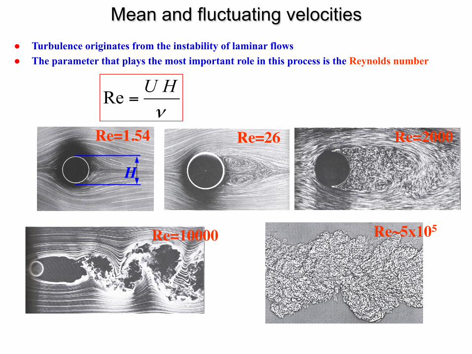
Mean and fluctuating velocities ● Turbulence originates from the instability of laminar flows ● The parameter that plays the most important role in this process is the Reynolds number
νHU
=Re
Re=26 Re=2000
Re=10000 Re~5x10⁵
Wake far behind the obstacle
Re=1.54
H U

Turbulence modeling ● We can think of turbulence as a
Ø Collection of eddies flowing Ø Largest eddies of size L and smallest eddies of size h Ø Eddies interact in a very complex manner Ø This interaction happens in a self-similar way
u Turbulent flow

Measuring mean and turbulent flow
'iii uuu +=
x z y
Free surface
ui = (u,v,w)

Measuring mean and turbulent flow
x z y
Free surface
ui = (u,v,w)
Instantaneous flow equations

Different Approaches to Modeling Turbulent Flows
Eddy size
Ener
gy d
ensi
ty
in
RANS
LES
DNS
out transfer
● DNS: direct numerical simulation (resolves all scales)
● LES: Large Eddy Simulation (resolves large and intermediate scales and models small scales)
● RANS: Reynolds Averaged Navier-Stokes (resolves large scales and models intermediate and small scales)

resolved modeled RANS
modeled resolved LES
resolved DNS C
ompu
tatio
nal c
ost i
ncre
ases
Scal
e of
sim
ulat
ion
incr
ease
s
Empi
rical
mod
elin
g in
crea
ses
Comparison of Modeling Approaches
Eddy size
Eddy
ene
rgy
in
out
RANS
LES DNS

LES (Large Eddy Simulation)

15 16
WSE WSE
Abad et al. (2013), ESPL
RANS modeling: KINOSHITA CHANNEL

Modeling in river-type systems
Eddy size
Mor
phod
ynam
ic
RANS
LES
DNS
1D, 2D and 3D flow models

3D flow equations
x z y
Free surface
Channel bottom
u,v,w
h
u(x,y,z),v(x,y,z),w(x,y,z) h(x,y,z)
[1] Mass conservation
[2] x-momentum
[3] y-momentum
[4] z-momentum

x z y
U,V Free surface
Channel bottom
h
U(x,y),V(x,y) h(x,y)
2D flow equations
[1] Mass conservation
[2] x-momentum
[3] y-momentum

x z y
U Free surface
Channel bottom
h
U(x) h(x)
1D flow equations 1.2. FLUID GOVERNING EQUATIONS 9
(Cf = 9.81n2h�1/3). Figure 1.7 shows an example where the depth-averagedform of the governing equations were used to simulate the fluid motion arounda bend (Abad et al., 2008a). Notice only horizontal velocities are computed.
1.2.3 One-dimensional (1D) form
Similarly, by integrating the 3D governing equation in a cross section, the 1Dcross-averaged governing equations are derived as:
@A
@t+
@Q
@x= 0 (1.9)
Figure 1.8: Example of simulation using 1D governing equations. Simulationperformed using HEC-RAS model
@Q
@t+
@
@x(�U2A) + gA
@h
@x= gA(So � Sf ) (1.10)
Where Q is the water discharge or flow rate, A is the cross-section area, � isthe momentum coe�cient, So and Sf are the bed and friction slopes respectively.Figure 1.8 shows an example where the 1D form of the governing equationswere used to simulate the hydrodynamics for the Matanza-Riachuelo creek inArgentina.
1.2. FLUID GOVERNING EQUATIONS 9
(Cf = 9.81n2h�1/3). Figure 1.7 shows an example where the depth-averagedform of the governing equations were used to simulate the fluid motion arounda bend (Abad et al., 2008a). Notice only horizontal velocities are computed.
1.2.3 One-dimensional (1D) form
Similarly, by integrating the 3D governing equation in a cross section, the 1Dcross-averaged governing equations are derived as:
@A
@t+
@Q
@x= 0 (1.9)
Figure 1.8: Example of simulation using 1D governing equations. Simulationperformed using HEC-RAS model
@Q
@t+
@
@x(�U2A) + gA
@h
@x= gA(So � Sf ) (1.10)
Where Q is the water discharge or flow rate, A is the cross-section area, � isthe momentum coe�cient, So and Sf are the bed and friction slopes respectively.Figure 1.8 shows an example where the 1D form of the governing equationswere used to simulate the hydrodynamics for the Matanza-Riachuelo creek inArgentina.
[1] Mass conservation
[2] x-momentum
Sediment Transport Processes And Sediment Conservation Equation (Exner)

Bed load and suspended load
suspended/wash load
bedload
Schmeeckle
( )Ecvqt
)1( bsbp −+⋅∇=∂
η∂λ−
-
ybyxbxb eqeqq +=
xy
z sediment bed

( ) 0455.0~037.0,7.5q c5.1
cb =ττ−τ= ∗∗∗∗
( )( ) 05.0,17q cccb =ττ−ττ−τ= ∗∗∗∗∗∗
( )( ) 05.0,7.074.18q cccb =ττ−ττ−τ= ∗∗∗∗∗∗
∗
∗−τ+
−τ−
−
+=
π− ∫
∗
∗
b
b2)/143.0(
2)/143.0(
t
q5.431q5.43dte11
2
( ) 03.0,12.11q c
5.4
c5.1b =τ⎟
⎟⎠
⎞⎜⎜⎝
⎛
τ
τ−τ= ∗
∗
∗∗∗
Fernandez Luque & van Beek (1976)
Ashida & Michiue (1972)
Engelund & Fredsoe (1976)
Einstein (1950)
Parker (1979) fit to Einstein (1950)
A BEDLOAD TRANSPORT RELATIONS FOR UNIFORM SEDIMENT (Parker’s e-book)
)(qqor)(qq cbbbb∗∗∗∗∗∗∗ τ−τ=τ=

19
1.E-09
1.E-08
1.E-07
1.E-06
1.E-05
1.E-04
1.E-03
1.E-02
1.E-01
1.E+00
1.E+01
1.E+02
0.01 0.1 1τ*
q b*
EAMEFFLBSandP approx EFLBGrav
PLOTS OF BEDLOAD TRANSPORT RELATIONS (Parker’s e-book)
E = Einstein AM = Ashida-Michiue EF = Engelund-Fredsoe P approx E = Parker approx of Einstein FLBSand = Fernandez Luque-van
Beek, τc* = 0.038 FLBGrav = Fernandez Luque-van
Beek, τc* = 0.0455

3D simulation - Hydrodynamic

1) EXISTING CONDITION: Lidar (2011)+MBES (2012)"
DATA"- Water slope and bed elevation calculation""
A slope of 1E-4 from gaging stations Mt. Carmel and New Harmony was calculated. Using that slope and the elevation of Mt. Carmel on February 2, 2012 a water surface was created for Maier Bend. Using the water surface and the MBES data the bed elevation surface was obtained.

FIELD MEASUREMENTS – WHAT DO WE NEED TO MEASURE?"

3D MODELING – MAIER BEND"
1) Existing condition – Lidar (2011)

3D MODELING – MAIER BEND"1) Existing condition - MBES (2012)

1) EXISTING CONDITION: Lidar (2011)+MBES (2012)"
DATA"- Water slope and bed elevation calculation""

1) EXISTING CONDITION: Lidar (2011)+MBES (2012)"
DATA"- MBES + Lidar + point bar (GPS)""

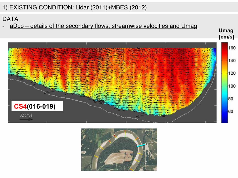
1) EXISTING CONDITION: Lidar (2011)+MBES (2012)"
DATA"- aDcp – details of the secondary flows, streamwise velocities and Umag""
CS3(011-014)
CS4(016-019)
CS5(021-024)
CS6(026-029)
CS10(044-045)
1) EXISTING CONDITION: Lidar (2011)+MBES (2012)"
DATA"- aDcp – details of the secondary flows, streamwise velocities and Umag""
CS4(016-019)
Umag [cm/s]

1) EXISTING CONDITION: Lidar (2011)+MBES (2012)"
DATA"- aDcp – details of the secondary flows, streamwise velocities and Umag"" Umag
[cm/s]
CS5(021-024)

1) EXISTING CONDITION: Lidar (2011)+MBES (2012)"
DATA"- aDcp – details of the secondary flows, streamwise velocities and Umag"" Umag
[cm/s]
CS6(026-029)

1) EXISTING CONDITION: Lidar (2011)+MBES (2012)"
DATA"- aDcp – details of the secondary flows, streamwise velocities and Umag"" Umag
[cm/s]
CS7(031-034)
1) EXISTING CONDITION: Lidar (2011)+MBES (2012)"
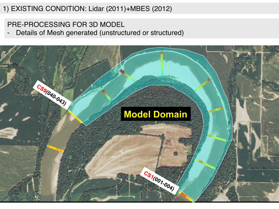
PRE-PROCESSING FOR 3D MODEL"- Details of Mesh generated (unstructured or structured)"
Model Domain

1) EXISTING CONDITION: Lidar (2011)+MBES (2012)"
PRE-PROCESSING FOR 3D MODEL"- Details of Mesh generated (unstructured or structured)"
Background Mesh Δs=2m Δn=2m Δz=0.5m
z s
n
Mesh was generated with OpenFOAM tool snappyHexMesh. It uses a background Hexahedral mesh and an STL surface to create the final mesh.
STL surface

1) EXISTING CONDITION: Lidar (2011)+MBES (2012)"
PRE-PROCESSING FOR 3D MODEL"- Details of Mesh generated (unstructured or structured)"
Mesh of hexahedral , polyhedra and pyramids elements
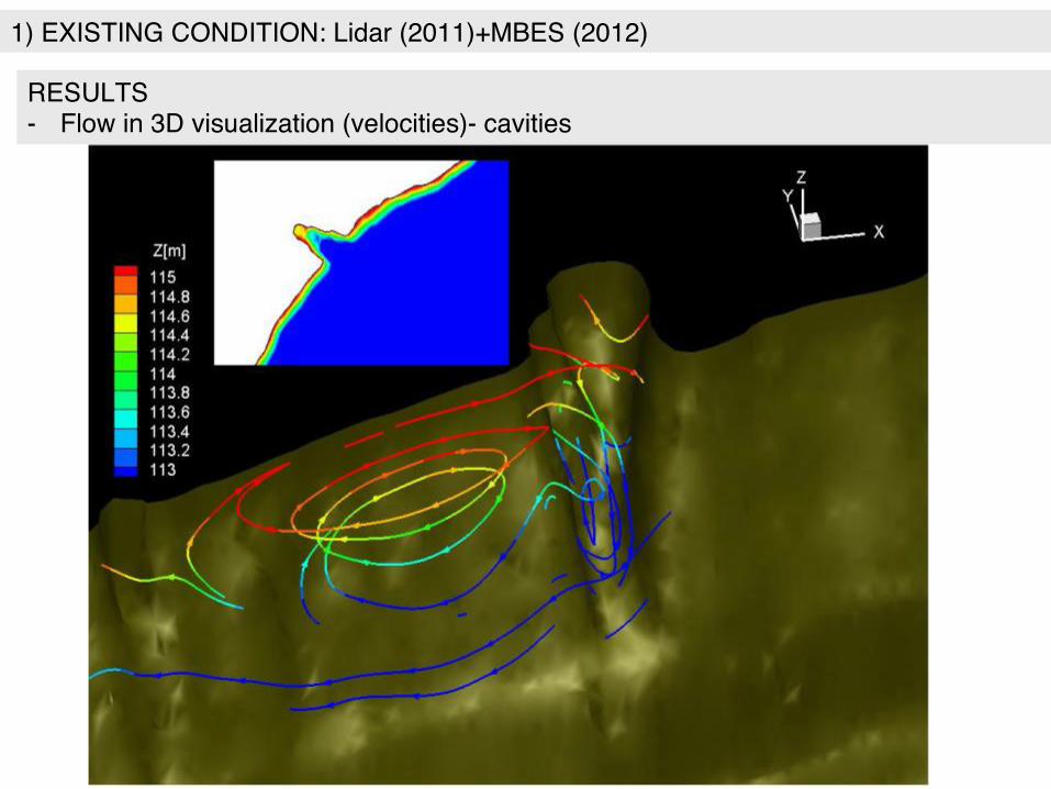
1) EXISTING CONDITION: Lidar (2011)+MBES (2012)"
RESULTS"- Flow in 3D visualization (velocities)- cavities "

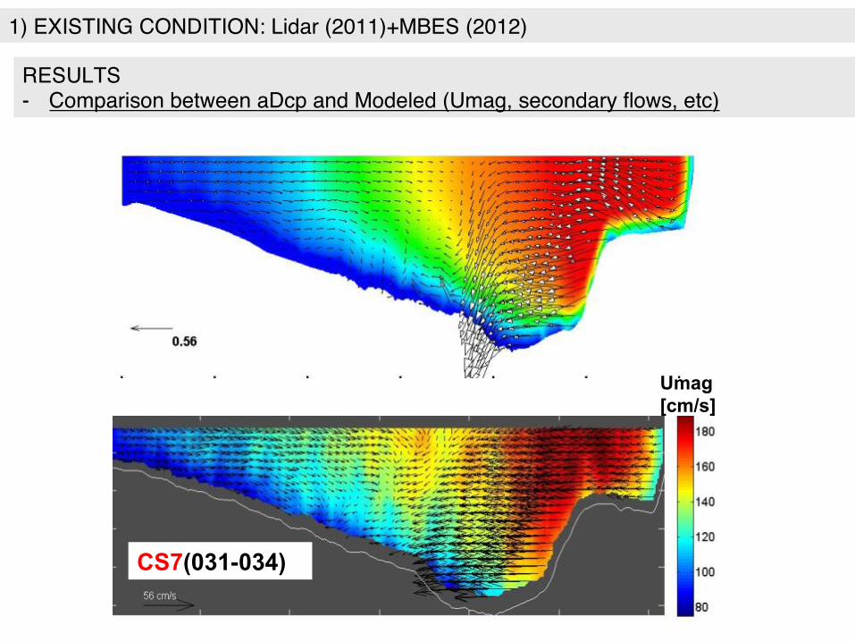
1) EXISTING CONDITION: Lidar (2011)+MBES (2012)"
RESULTS"- Comparison between aDcp and Modeled (Umag, secondary flows, etc)"
CS6(026-029)
Umag [cm/s]
1) EXISTING CONDITION: Lidar (2011)+MBES (2012)"
RESULTS"- Comparison between aDcp and Modeled (Umag, secondary flows, etc)"
CS7(031-034)
Umag [cm/s]

1) EXISTING CONDITION: Lidar (2011)+MBES (2012)"
RESULTS"- Comparison between aDcp and Modeled (Umag, secondary flows, etc)"
Umag [cm/s]
CS8(036-039)
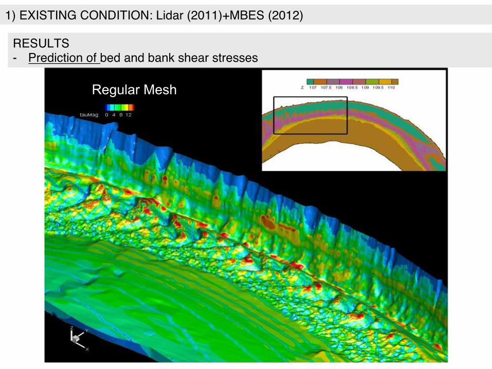
1) EXISTING CONDITION: Lidar (2011)+MBES (2012)"
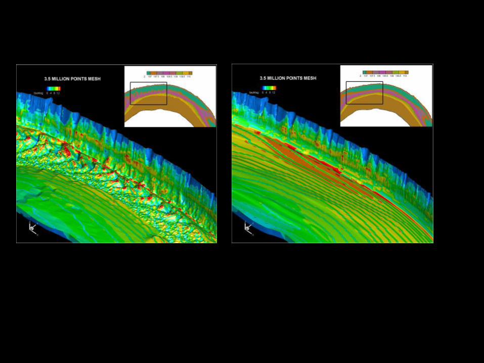
RESULTS"- Prediction of bed and bank shear stresses"
Regular Mesh

1) EXISTING CONDITION: Lidar (2011)+MBES (2012)"
RESULTS"- Prediction of bed and bank shear stresses"
Fine Mesh
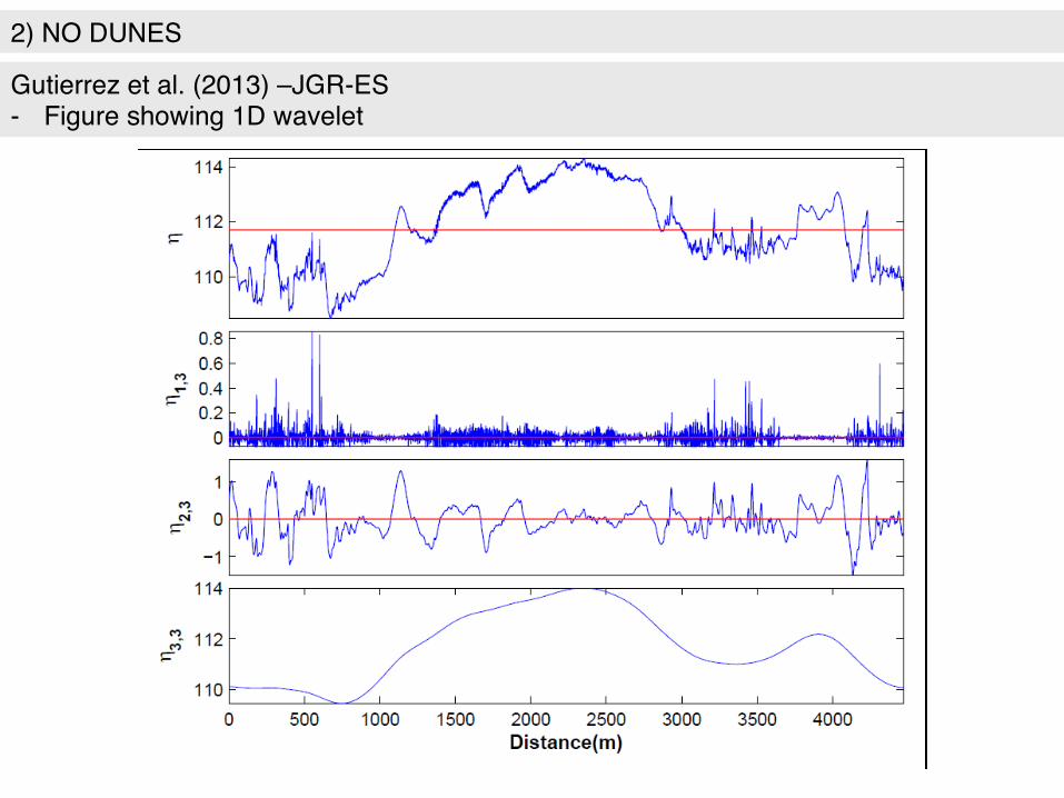
2) NO DUNES"
Gutierrez et al. (2013) –JGR-ES"- Figure showing 1D wavelet"

2) NO DUNES"
Gutierrez et al. (2013) –JGR-ES"- Figure showing 3D bed – not working"

2) NO DUNES"
Gutierrez et al. (2013) –JGR-ES"- Figure showing smoothed bed condition"

2) NO DUNES"
Gutierrez et al. (2013) –JGR-ES"- Figure showing the mesh"


Steady + unsteady bed morphology

η(t) = <η> + η’(t) <η>
η’(t)
Dunes

η(t) = <η> + η’(t)
<η>
η’(t) Bed profiles at centerline
<qb> ~ 9.68E-07 m2/s
<qb> qb’
Bed load fluxes
qb(t) = <qb> + qb’(t)

Steady (Point bars) + perturbed components (bars)

1D SEDIMENT TRANSPORT MORPHODYNAMICS with applications to
RIVERS AND TURBIDITY CURRENTS © Gary Parker November, 2004
51
TOUR OF BEDFORMS IN RIVERS: ALTERNATE BARS
Alternate bars in the Naka River, an artificially straightened river in Japan. Image courtesy S. Ikeda.
Alternate bars occur in rivers with sufficiently large (> ~ 12), but not too large width-depth ratio B/H. Alternate bars migrate downstream, and often have relatively sharp fronts. They are often precursors to meandering. Alternate bars may coexist with dunes and/or antidunes.

1D SEDIMENT TRANSPORT MORPHODYNAMICS with applications to
RIVERS AND TURBIDITY CURRENTS © Gary Parker November, 2004
52
BEDFORMS IN THE LABORATORY AND FIELD: ALTERNATE BARS Alternate bars in a flume in Tsukuba University, Japan: flow turned low.
Image courtesy H. Ikeda.
Alternate bars in the Rhine River between Switzerland and Lichtenstein.
Image courtesy M. Jaeggi.

1D SEDIMENT TRANSPORT MORPHODYNAMICS with applications to
RIVERS AND TURBIDITY CURRENTS © Gary Parker November, 2004
53
BEDFORMS IN THE LABORATORY AND FIELD: MULTIPLE-ROW (LINGUOID) BARS
Linguoid bars in a flume in Tsukuba University, Japan: flow turned off.
Image courtesy H. Ikeda. Linguoid bars in the Fuefuki River, Japan. Image courtesy S. Ikeda.

ρs=2566.5 Kg/m3
Grain Size Distribution
0
10
20
30
40
50
60
70
80
90
100
0.1 1 10Grain size (mm)
Perc
ent f
iner
D50=0.832 mm
Dg=0.828 mmσ
g=1.234<1.60 (well sorted)
λp=0.4 ( ) encsq *** ττφα −=
Designing the experiments: Obtaining βC and βR à Sediment transport
β
λπ 02 hk =cc k,βRR k,β

Lisle et al. (1997)
Free bars in straight channels
λ
B2
Free bars regime
Pool
Pool
Pool
Pool Free bars in HAMC
Whiting and Dietrich (1993)


Modeling of forced and free bars Alejandro Mendoza (Postdoc)
Point bars Free bars

Tools 2D 3D
• Telemac-‐Mascaret http://www.opentelemac.org/
• Mike 21C http://mikebydhi.com/Products/WaterResources/MIKE21C.aspx
• Delft 3d http://www.deltaressystems.com/hydro/product/621497/delft3d-‐suite

Bed Morphology
• Telemac-‐2D – Solves St. Venant equations – Utilizes FEM in irregular grids
• Sisyphe – Computes sediment transport with empirical formulas
– Applies corrections for bed/bedforms effects and secondary flows when using Telemac-‐2D

FORCED BARS Hooke experiments

Hooke experiments
After Hooke (1975) (Journal of Geology)

Experiments
• Q = [10-‐50.5] l/s • Recirculated sediment • diameter = 0.30 mm • Density = 2700 kg/m3

Mesh and Boundary Conditions
HQL
QS
Inlet Outlet
Friction coefficient
Sediment roughness

Sediment transport
• qs = 2E-‐6 m2/s (from experiments)
• Calibration using different equations
• Roughness of sediment particles
• Use of corrections for bed slope and particle trajectory
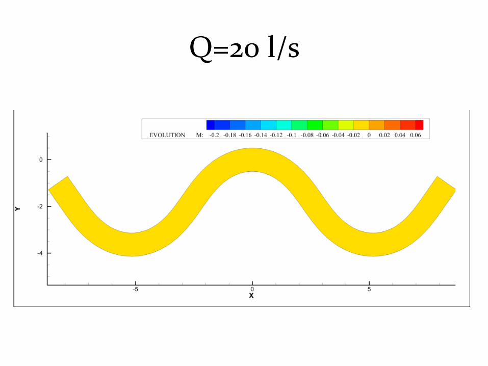
Q=20 l/s

Q=50.5 l/s

Results for Q=20 l/s
Hooke (1975) (Journal of Geology)

FREE BARS Lanzoni Experiments

Lanzoni (2000a) WRR • Development of alternate bars in ripple and/or covered beds
• Flume 55 m long 1.5 m wide • Sediment recirculation, • Qs = 1.05E-‐5 m2/s (converted from Qs = 94.5 l/h pores included)
• Sediment characteristics – d = 0.48 mm – ρ = 2650 kg/m3 – Q = [25-‐47] l/s

More experiments for free bars
• Modeling is done with Telemac-‐2D and Sisyphe • Equation selected was Meyer-‐Peter and Mueller. Since Telemac computes µ = c’f/cf with c’f from skin friction calculated with Nikuradse, the sediment transport in Sisyphe was calibrated with ks = 3.6D50

Sediment recirculation
Q= 30 l/s Initial perturbation: Bump in the inlet

Bed evolution
Lanzoni [2000a] (Table 2, run 1505) Wavelength = 10.0m Bar height = 7.7 cm celerity = 2.8 m/h

72 HRS SIMULATION
Since bars are advected together with the bump, a permanent perturbation is needed

Results
• Evolution of the bed, right bank • Profiles every 60 min. • Wavelength 10 m aprox. (Lanzoni
measured 10m) • Celerity 2.2 m/h (Lanzoni
measured 2.8 m/h) • Bar height 8 cm (7.7 from
Lanzoni)

Important aspects for bed morphology modeling
• Measurements of sediment transport from field
• Calibrate the sediment equation in order to reproduce measurements

RVR Meander (www.rvrmeander.org)
Jorge D. Abad1, Davide Mo:a2, Eddy J. Langendoen3, Roberto Fernandez2, Nils O. Oberg2, Marcelo H. Garcia2
4River Centerline
Valley Centerline
RVR Meander User Interface
0
5
10
15
20
25
30
35
MigratedCenterlines (yrs)
2D Output
1.1 - 1.5
0.8 - 1.1
0.5 - 0.8
1.1 - 1.3
0.8 - 1.1
0.5 - 0.8Velo
city
Mag
nitu
de (m
/s)
After 5 years After 35 years
2.1 - 3.5
0.6 - 2.1
-0.9 - 0.6
1.9 - 3.2
0.6 - 1.9
-0.8 - 0.6
Wat
er D
epth
(m)
11.9 - 16.6
7.1 - 11.9
2.3 - 7.1
9.7 - 13.4
5.9 - 9.7
2.2 - 5.9
Shea
r Str
ess
Mag
nitu
de (P
a)
1D Output
Floodplain HeterogeneityBasic Input
1 Dept. of Civil and Environmental Engineering, University of Pittsburgh 2 Ven Te Chow Hydrosystems Laboratory, Dept. of Civil and Environmental Engineering, University of Illinois at Urbana-Champaign 3 USDA-ARS National Sedimentation Laboratory, Oxford, Mississippi

Meandering scales Somewhere near Detroit
Pictures courtesy Eddy Langendoen
λv Α

Meandering scales (λ) With the ongoing effort in both the United States and Europe to re-‐naturalize highly modified streams à more development of GIS Engineering Tools are needed
Proposed alignments for re-‐meandering of Trout Creek, Lake Tahoe, California.
US reach - Predesign
US reach - Design
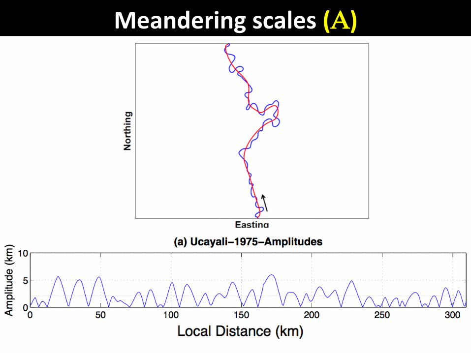
Meandering scales (Α)

Meandering scales – free? Near Fargo, ND (Red River)

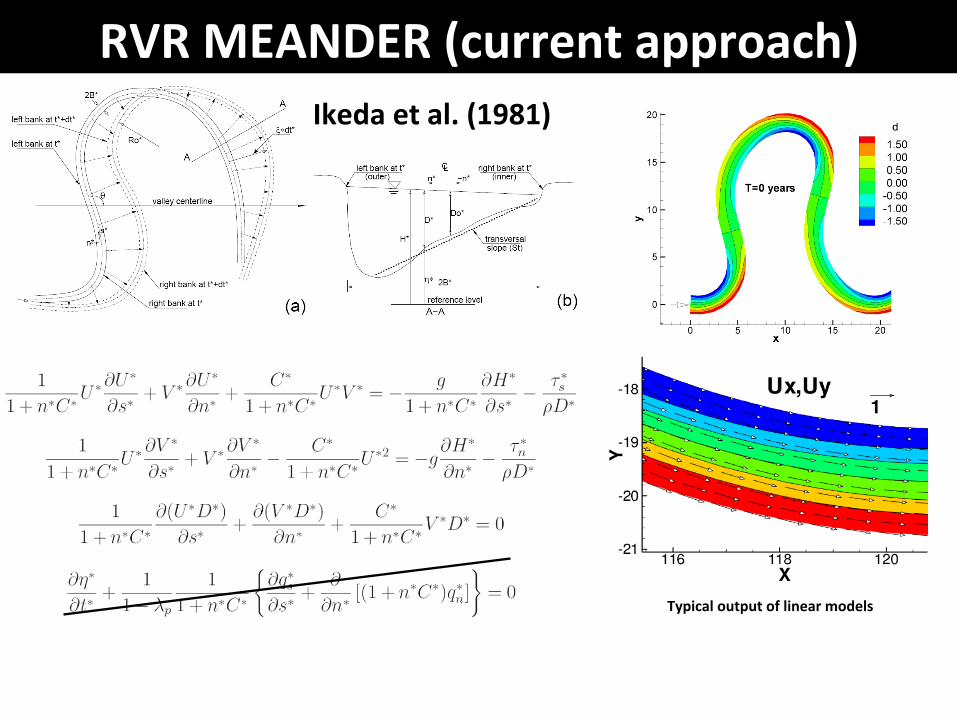
RVR MEANDER (classical approach)
Typical output of linear models
Ikeda et al. (1981)

RVR MEANDER (the classical approach) Classic migraZon-‐coefficient method for migraZon (Ikeda et al. 1981)
The coefficient E0 is usually obtained via calibraSon against historic channel centerlines.
LimitaZons of classic approach based on calibrated migraZon coefficient: q it predicts a smooth and “conSnuous” migraSon pa:ern; q linearity of the expression: it does not explicitly account for local, episodic mass failure mechanisms; q the formulaSon does not account for an erosion threshold; q it does not consider the effect of the bank geometry either; q it does not consider the impact of the verScal heterogeneity of the bank materials, horizontal could be incorporated changing Eo

Hickin, E. J. (1974). The development of meanders in natural river channels: American Journal of Science, 274, 414-442
Complex planform pa_erns

RVR Meander: simplified two-‐dimensional (2D) hydrodynamic and migraSon model (Abad and Garcia, 2006), based on migraSon coefficient approach
RVR MEANDER (current approach) The RVR Meander pla_orm merges the funcSonaliSes of the first version of MEANDER (Garcia, Bi:ner, and Nino, 1994) and RVR Meander (Abad and Garcia, 2006) with CONCEPTS (Langendoen and Simon, 2008).
CONCEPTS (CONservaSonal Channel EvoluSon and Pollutant Transport System): one-‐dimensional (1D) hydrodynamic and morphodynamic model (Langendoen and Alonso, 2008; Langendoen and Simon, 2008; Langendoen et al., 2009)
The new plaborm q is wri:en in C++ language; q is composed of different libraries (preprocessing, hydrodynamics, bank erosion, migraSon, filtering, plofng, and I/O); q stand-‐alone for Windows and Linux operaSng systems and interface in ArcGIS-‐ArcMap.
RVR MEANDER (current approach)
Typical output of linear models
Ikeda et al. (1981)
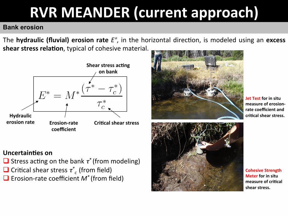
The hydraulic (fluvial) erosion rate E∗, in the horizontal direcSon, is modeled using an excess shear stress relaZon, typical of cohesive material.
Bank erosion
Jet Test for in situ measure of erosion-‐rate coefficient and criZcal shear stress.
Cohesive Strength Meter for in situ measure of criZcal shear stress.
Erosion-‐rate coefficient
CriZcal shear stress
RVR MEANDER (current approach)
UncertainZes on q Stress acSng on the bank τ* (from modeling) q CriScal shear stress τ*c (from field) q Erosion-‐rate coefficient M* (from field)
Hydraulic erosion rate
Shear stress acZng on bank

Bank materials composed of fine-‐grained cohesive sediments. Bank erosion: combinaSon of fluvial shear erosion and gravitaZonal mass failure processes. Depending on shape of bank profile and physical properSes of the bank materials, any one of the following mass failure mechanisms might be observed
q planar q rotaSonal q canSlever q piping or sapping
Planar failure Planar failure
RotaZonal failure
CanZlever failure Piping
RVR MEANDER (current approach)
Pictures courtesy Eddy Langendoen

Mo:a, D., Abad, J.D, Langendoen, E.J., Garcia, M.H., 2011. A simplified 2D model for meander migra:on with physically-‐based bank evolu:on. Geomorphology
[1] RVR MEANDER: MC vs PB
Aerial pictures of the Mackinaw River in the years 1951 and 1988.
Reach of the Mackinaw River in Illinois located in Tazewell County about 15 kilometers upstream of the juncSon of the Mackinaw River with the Illinois River.
Mackinaw River study reach.
flow
flow

The proposed approach showed significant improvements over the classic approach in predicSng the observed migraSon in the period 1951-‐1988, both in terms of
q shapes q predicZon error
q Compound loops are captured by PB
Test for natural river
Mackinaw River study reach: historic and predicted centerlines in 1988. Flow is from right to lei (Mo_a et al., 2011).
flow
flow
flow
MC2
MC1
PB
[1] RVR MEANDER: MC vs PB

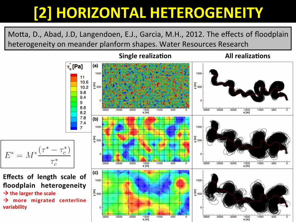
Mo:a, D., Abad, J.D, Langendoen, E.J., Garcia, M.H., 2012. The effects of floodplain heterogeneity on meander planform shapes. Water Resources Research
[2] HORIZONTAL HETEROGENEITY
Single realizaZon All realizaZons
Mo:a, D., Abad, J.D, Langendoen, E.J., Garcia, M.H., 2012. The effects of floodplain heterogeneity on meander planform shapes. Water Resources Research
[2] HORIZONTAL HETEROGENEITY
Single realizaZon All realizaZons
Effects of length scale of floodplain heterogeneity à the larger the scale à more migrated centerline variability

Mo:a, D., Abad, J.D, Langendoen, E.J., Garcia, M.H., 2012. The effects of floodplain heterogeneity on meander planform shapes. Water Resources Research
[2] HORIZONTAL HETEROGENEITY
High-‐frequency meander bends are starZng to appear
Single realizaZon Single realizaZon

Vertically homogeneous
Tblock = 50 daysVertically heterogeneous
Station [m]
Elevation[m]
-17 -16 -15 -14 -13
-3
-2
-1
0
1
2
2 layers with different erodibility
Layer 1
Layer 2
Station [m]
Elevation[m]
-17 -16 -15 -14 -13
-3
-2
-1
0
1
2
2 layers with same erodibility
Layer 2
Layer 1
VerZcal heterogeneity affects canZlever failure volumes and therefore migraZon Homogeneous migrates at higher rates
Area of vertical heterogeneity for erodibility
[3] VERTICAL HETEROGENEITY
wse
wse
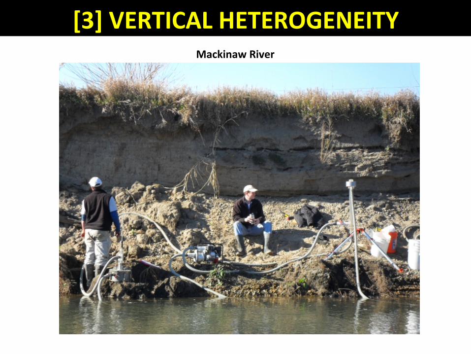
[3] VERTICAL HETEROGENEITY Mackinaw River

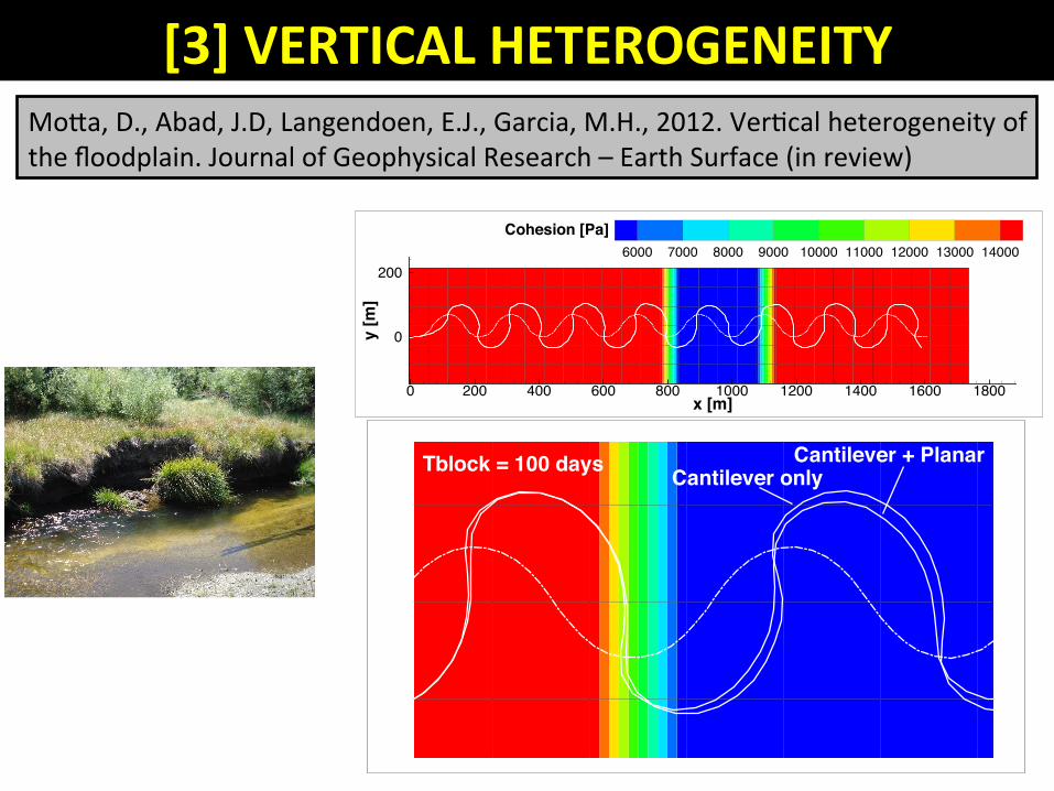
Mo:a, D., Abad, J.D, Langendoen, E.J., Garcia, M.H., 2012. VerScal heterogeneity of the floodplain. Journal of Geophysical Research – Earth Surface (in review)
[3] VERTICAL HETEROGENEITY
X - 20MOTTA ET AL.: MEANDER MIGRATION IN HORIZONTALLY AND VERTICALLY HETEROGENEOUS FLOODPLAINS
Figure 1. Examples of slump blocks in rivers characterized by di!erent spatial scales.
(a) Small scale: Trout Creek (California, USA), with small blocks but long residence
time; (b) Intermediate scale: Mackinaw River (Illinois, USA), with larger but less present
blocks; c Large scale: Pilcomayo River (Argentina), blocks are substantially absent.
D R A F T January 22, 2012, 5:31pm D R A F T
X - 24MOTTA ET AL.: MEANDER MIGRATION IN HORIZONTALLY AND VERTICALLY HETEROGENEOUS FLOODPLAINS
x [m]
y [m
]
0 200 400 600 800 1000 1200 1400 1600 1800
0
2006000 7000 8000 9000 10000 11000 12000 13000 14000
Cohesion [Pa]
Tblock
500100
Figure 6. Impact of slump block existence period on meander migration. Comparison
between Tblock = 100 and 500 days.
D R A F T January 22, 2012, 5:31pm D R A F T
[3] VERTICAL HETEROGENEITY
MOTTA ET AL.: MEANDER MIGRATION IN HORIZONTALLY AND VERTICALLY HETEROGENEOUS FLOODPLAINSX - 25
x [m]
y [m
]0 200 400 600 800 1000 1200 1400 1600 1800
0
2006000 7000 8000 9000 10000 11000 12000 13000 14000
Cohesion [Pa]
Cantilever + PlanarTblock = 100 days Cantilever only
Figure 7. Relative importance of cantilever and planar failure.
D R A F T January 22, 2012, 5:31pm D R A F T
X - 20MOTTA ET AL.: MEANDER MIGRATION IN HORIZONTALLY AND VERTICALLY HETEROGENEOUS FLOODPLAINS
Figure 1. Examples of slump blocks in rivers characterized by di!erent spatial scales.
(a) Small scale: Trout Creek (California, USA), with small blocks but long residence
time; (b) Intermediate scale: Mackinaw River (Illinois, USA), with larger but less present
blocks; c Large scale: Pilcomayo River (Argentina), blocks are substantially absent.
D R A F T January 22, 2012, 5:31pm D R A F T
Mo:a, D., Abad, J.D, Langendoen, E.J., Garcia, M.H., 2012. VerScal heterogeneity of the floodplain. Journal of Geophysical Research – Earth Surface (in review)

www.rvrmeander.org
SHORT COURSES q R i v e r C o a s t a l a n d E s t u a r i n e
Morphodynamics, RCEM 2009, Santa Fe, ARGENTINA
q NaSonal University of Engineering, NaSonal Congress 2010, Lima, Cusco, PERU
q R i v e r C o a s t a l a n d E s t u a r i n e Morphodynamics, RCEM 2011, Tsinghua University, Beijing, CHINA
q USDA-‐FOREST – LAKE TAHOE, Dec 2011, Nevada.
q UNAM-‐Mexico, January 2013

www.rvrmeander.org
THANKS

LinearizaZon
Dimensionless perturbaZons of velocity in the streamwise and transverse direcZon and water depth
Important parameters:
q Sinuosity q Half width-‐to-‐depth raSo q Froude number q FricSon coefficient
Hydrodynamics and bed morphodynamics (contd.)
Dimensionless transverse velocity perturbaZon
Dimensionless depth perturbaZon
Dimensionless streamwise velocity perturbaZon
Reach-‐averaged values PerturbaZons
RVR MEANDER

The canZlever failure is associated to overhanging slumps of mass generated by preferenSal retreat of highly erodible layers or simply by the erosion of the bank below the water level with respect to its dry porSon. The occurrence of canSlever failure is determined from geometrical consideraSons, once an undercut threshold is exceeded.
Layer i
Layer i+1
Failure surface
Time
Hydraulic erosion
Bank erosion (contd.)
Sketch of canZlever failure.
RVR MEANDER
RVR Meander
GIS interface
Interface overview
Live demonstraSon
Future work
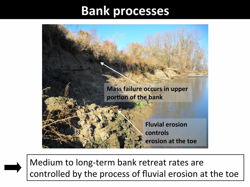
Fluvial erosion controls erosion at the toe
Mass failure occurs in upper porZon of the bank
Bank processes
Medium to long-‐term bank retreat rates are controlled by the process of fluvial erosion at the toe

Bank armoring
Increasing river scale
Bank processes
Mass failure mechanisms may impact migraSon rates and shapes through bank toe protecSon
Trout Creek, USA Mackinaw River, USA Pilcomayo, ArgenZna
River scale may affect residence Sme of slump blocks

Layering impacts mass failure volumes
Impacts bank protecSon
Impacts migraSon rates and shapes
Bank processes Bank layering
VerScal heterogeneity in the floodplain may impact migraSon rates and shapes