MODEL VERIFICATION OF THREE-DIMENSIONAL · PDF fileDepartment of Mechanical Engineering ......
102
(NASA —CR-165623 — Vol-4) THERMAL POLLUTION N81-23557 MATHEMATICAL MODEL. VOLUME 4. VERIFICATION OF THREE — DIMENSIONAL RIGID — LID MODEL AT LAKE KEOWEE Final Report (Miami Univ.) 102 p Unclas HC A06/MF A01 CSCL 13B G3/43 23982 Final Report THERMAL POLLUTION MATHEMATICAL MODEL (Volume Four of Seven Volumes) VERIFICATION OF THREE-DIMENSIONAL RIGID-LID MODEL AT LAKE KEOWEE Volume IV RECEIVED NASA STl FACIUTy ACCESS DEPT. by Samuel S. Lee, Subrata Sengupta, Emmanuel V. Nwadike and Sumon K. Sinhe Department of Mechanical Engineering University of Miami Coral Gables, Florida 33124 Prepared for National Aeronautics and Space Administration and Environmental Protection Agency (NASA Contract NAS 10-9410) August 1980 _. https://ntrs.nasa.gov/search.jsp?R=19810015023 2018-05-19T06:29:01+00:00Z
Transcript of MODEL VERIFICATION OF THREE-DIMENSIONAL · PDF fileDepartment of Mechanical Engineering ......

(NASA—CR-165623—Vol-4) THERMAL POLLUTION N81-23557MATHEMATICAL MODEL. VOLUME 4. VERIFICATIONOF THREE— DIMENSIONAL RIGID—LID MODEL AT LAKEKEOWEE Final Report (Miami Univ.) 102 p UnclasHC A06/MF A01 CSCL 13B G3/43 23982
Final Report
THERMAL POLLUTION MATHEMATICALMODEL
(Volume Four of Seven Volumes)
VERIFICATION OF THREE-DIMENSIONALRIGID-LID MODEL AT LAKE KEOWEE
Volume IV
RECEIVEDNASA STl FACIUTy
ACCESS DEPT.
by
Samuel S. Lee, Subrata Sengupta,Emmanuel V. Nwadike and Sumon K. Sinhe
Department of Mechanical EngineeringUniversity of Miami
Coral Gables, Florida 33124
Prepared for
National Aeronautics and Space Administrationand
Environmental Protection Agency(NASA Contract NAS 10-9410)
August 1980
- -- _. -
https://ntrs.nasa.gov/search.jsp?R=19810015023 2018-05-19T06:29:01+00:00Z

Kec room to-VaNs ^Rtv 7-7e1
STANDARD TITLE PAGE
1. Report No. 2. Government Accession Me. 3. Recipient's Catalog No
CR-1656234. Title and Subtitle 3. Report Date
Thermal Pollution Math Model Volume IV,Verification of Three-Dimensional Rigid-Lid 6. Performing Organization Code
Model at Lake Keowee TR 43-47. Author(s) Drs. Samuel Lee and Subrata engupta; S. Performing Organisation Report No.
Emmanuel V. Nwadike and Sumon K. Sinha9. Performing Organisation Name end Address 10. Work Unit No.
John F. Kennedy Space Center 11. Contract er Grant No.Kennedy Space Center, Florida 32899Project Manager: Roy A. Bland Code PT-FAP NAS10••9410
13. Type of Report and Period Covered
12. Sponsoring Agency Name and Address
National Aeronautics and Space Administration Finaland Environmental Protection AgencyResearch Triangle Park, N.C.
14. Sponsoring Agency Cod•
15. AbstractThe Rigid Lid was developed by the University of Miami, Thermal Pollution
Group, to predict three-dimensional temperature and velocity distributions
in lakes. This model was verified at various sites (Lake Belews, Biscayne Bay,etc.) and the verification at Lake Keowee was the last of these series ofveri fication runs.
The verification at Lake Keowee included the following phases of work.
1. Selecting the domain of interest, grid systems and comparing thepreliminary results with archival data.
2. Obtaining actual ground truth and infrared scanner data both for summerand winter.
3. Using the model to predict the measured data for the above periods and
comparing the predicted results with the actual data.
The model results have compared well with measured data. Thus, the model can
be used as an effective predictive tool for future sites.
16, Key WordsThermal Pollution Waste Heat
Math ModelsNuclear or Fossil Fuel Power Plants
17. Bibliographic Control 10. Distribution
Announce in Star Unlimited
Category 43
19. secunty Class.f.iol th-s roport) i 20. secv nty closs.l.kof tn,s page) 21. No. of Pages 22. Pnce
None None

PREFACE
The Thermal Pollution Group at the University of Miami has beendeveloping three-dimensional mathematical models for predicting thehydrothermal behaviors of bodies of water subjected to a heated effluent.Generally speaking, these models can be classified in two categories,namely, the free surface models which take into account the variationIn water surface elevations and rigid-lid models which treat the watersurface as flat.
To enable the prospective user to use these models as accuratepredictive tools, particularly to assess the environmental impact in thecase of cooling lakes, they have to be calibrated and verified at a num-ber of sites. The present volume describes the application of the rigid-lid model developed by this group to a rather complicated site, namely,Lake Keowee in South Carolina. Lake Keowee is rather unique sinceit is used by a Nuclear Power Plant as a cooling lake as well as twoother hydroelectric stations which use it as lower and upper ponds.
This is the final verification of these models concluding a series ofsuch verifications made possible by funding and technical assistanceprovided by the National Aeronautics and Space Administration (NASA)and the Environmental Protection Agency (EPA) .
This model will eventually be made available to all prospectiveusers by NASA and EPA. The present volume together with the"Three Dimensional Rigid-Lid Model User's Manual" is intended forassisting such future users.
ABSTRACT
The Rigid Lid was developed by the University of Miami, ThermalPollution Group, to predict three-dimensional temperature and velocitydistributions in lakes. This model was verified at various sites (LakeBelews, Biscayne Bay, etc.) and the verification at Lake Keowee wasthe last of these series of verification runs.
The verification at Lake Keowee included the following phases ofwork.
1. Selecting the domain of interest, grid systems and comparingthe preliminary results with archival data.
2. Obtaining actual ground truth and infrared scanner data both forsummer and winter.
3. Using the model to predict the measured data for the above periodsand comparing the predicted results with the actual data.
The model results have compared well with measured data. Thus,the model can be used as an effective predictive tool for future sites.
iii
CONTENTS
Preface ......................................................... IfAbstract ........................................................ iii
Figures ......................................................... v
Tables .......................................................... viii
Symbols ........................................................ ix
Acknowledgments ................................................ x
I. Introduction ........................................... 1
Background....................................... 1Objectives of present work ...................... 1Description of Lake Keowee site 2
2. Conclusions ............................................ 33. Recommendations ............. 44. Mathematical Formulation and Model Description ......... 5
Choiceof model ................................ 5Description model .............................. 5Governingequations .............................. 6
Initial and boundary conditions .................... 9Spatial difference schemes ......................... 11Stability ........................................ 12
Markermatrices ................................... 125. Application to Lake Keowee ........................... 14
Introduction........................... 14Choice of domain and grid system ................. 14Summaryof data .................................. 15Calculation of input ............................... 18
6. Results and Discussions ................................ 23
References...................................................... 29
IV
FIGURES
N umber
1 Lake Keowee ............................................
2 Grid system for the rigid-lid model .....................
3 MAR markers matrix (main grid points) ..................
4 MRH marker matrix (half grid points) ...................
5 Map of area of interest .................................
6 Measured isotherms (archival 9/10/75) ...................
7 August ground truth data (measuring stations) ..........
8 Flight plans for IR data (August and February missions) .
9 Keowee hydro discharge data (August 24, 1978) .........
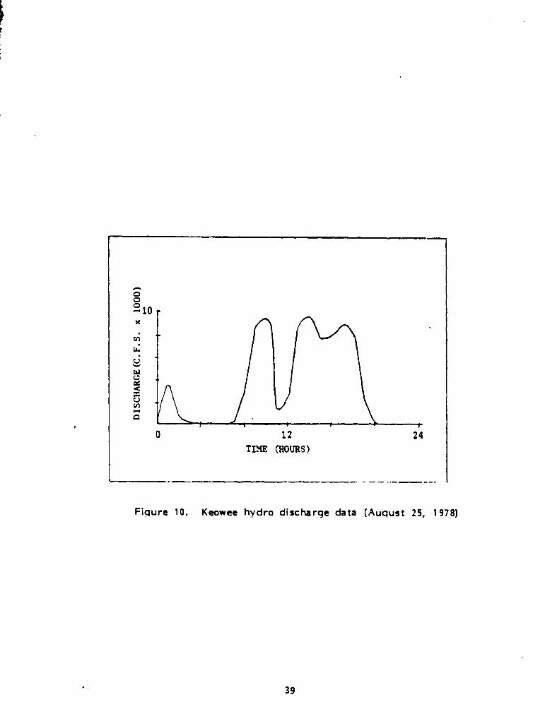
10 Keowee hydro discharge data (August 25, 1978) .........
11 Jocassee-pumped storage station discharge data(August 24, 1978) ................................ .....
12 Jocassee-pumped storage station discharge data(August 25, 1978) ......................................
13 Keowee February 1979 showin g stations .................
14 Jocassee-pumped storage station discharge data(February 27, 1979) .....................................
15 Jocassee-pumped storage station discharge data(February 28, 1979) .....................................
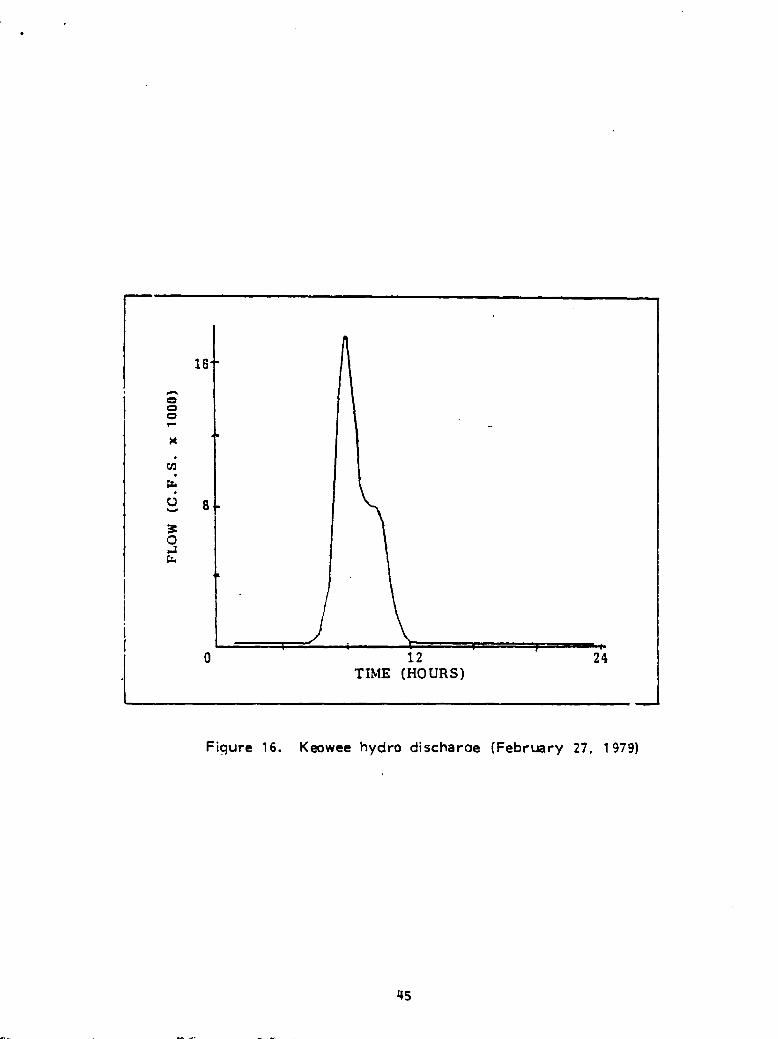
16 Keowee hydro discharge (February 27, 1979) ............
17 Keowee hydro discharge (February 28, 1979) ............
18 Velocities at K = 1 after 8.64 hrs. (1-001) ...............
v
Page
30
31
32
33
34
35
36
37
38
39
40
41
42
43
44
45
46
47

FIGURES
Number Page
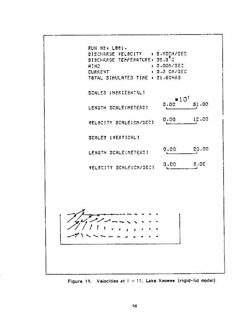
19 Velocities at I = 11 after 21.6 hrs. (1-001) ............... 48
20 Isotherms measured and predicted after 8.64 hrs. (1-001) . 49
21 Velocities at K = 1 after 8.64 hrs. (1-002) ............... 50
22 Velocities at 1 = 11 after 8.64 hrs. (1-002) ....... ....... 51
23 Isotherms measured and predicted after 8.64 hrs. (1-002) . 52
24 Velocities at K = 1 after 8.00 hrs. (LO03) ............... 53
25 Velocities at J = 7 after 4.32 hrs. (LO03) ............... 54
26 Isotherms measured and predicted after 8.64 hrs. (LO03) . 55
27 Isotherms measured and predicted (LO04) ................ 56
28 Velocities at K = 1 after 4. 32 hrs. (LOOS) ................ 57
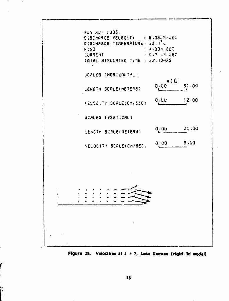
29 Velocities at J = 7 after 32.4 hrs. (LOOS) ................ 58
30 Isotherms measured and predicted after 32.40 hrs. (LOOS) 59
31 Vertical temperature profiles (LOOS) ..................... 60
32 Comparison of surface velocities (I = 11, J = 7, K = 1) .. 61
33 Comparison of surface velocities (I = 11, J = 2, K = 1) .. 62
34 I R Data corresponding to 1002 hrs., August 24, 1978 ... 63
35 Surface isotherms 1002 hrs. , August 24, 1978(30.5, 30.0, 29.5°C) .................................... 64
36 Surface isotherms 1002 hrs., Auaust 24, 1978(29.5, 29.3, 29.1°C) .................................... 65
37 IR data corresponding) to 0903-0953 hrs., Auaust 25, 1978. 66
38 Surface isotherms 1 3. 23 hrs. , Auaust 25, 1978(30.0, 29.5°C) .......................................... 67
39 Surface isotherms 33.2 hrs. , August 25, 1973(29.90, 29.70, 29.60°C) ................................. 68
vi

F
FIGURES
Number Pacae
40 Velocities at K = 1, 10. 07 hrs. , Aucaust 25, 1978........... 69
41 Velocities at K = 1, 34. 24 hrs. , Aug ust 25, 1978 ...... 70
42 IR data corresponding to 1648-1651 hrs.,February 27, 1979 ...................................... 71
43 Surface isotherms 17.12 hrs., February 27, 197?(1 3.0, 12.75, 12. 5,1 2.0, 1 1. 5, 11.0°C) ..................... 72
44 Surface isotherms 17.12 hrs. , February 27, 1979(13.75, 13.0, 12.5, 12.0°C) ........... ................. 73
45 IR data corresponding to 0948-0957 hrs.,February 28, 1979 . .................. .................. 74
46 Surface isotherms 34.2 hrs., February 28, 1979(13.0, 12.5°C) .......................................... 75
47 Velocities at K = 1, 17.12 hrs., February 27, 1979 ...... 76
48 Velocities at K = 1, 34. 24 hrs. , February 28, 1979 ...... 77
vii
S y

TABLES
Number
Pag^
1 Monthly Gross Thermal Capacity Factors ofOconee Nuclear Station .... 78
2 Operating Conditions of Oconee Nuclear
Power Plant (September 10, 1975) ....................... 79
3 Input Data for 3-D Model (Lake Keowee) ................. 80
4 Volume and Area Data for Lake Keowee ................. 81
5 Inflows and Outflows to Lake Keowee, August 24, 1978 .. 82
6 Inflows and Outflows to Lake Koewee, August 25, 1978 .. 83
7 Meteorological Data for Lake Keowee, August 24, 1978 ... 84
8 Meteorological Data for Lake Keowee, August 25, 1978 ... 85
9 Inflows and Outflows to Lake Keowee, February 27, 1979 . 86
10 Inflows and Outflows to Lake Keowee, February 28, 1979.
87
11 Meteorological Data for Lake Keowee, February 27, 1979 .. 88
12 Meteorological Data for Lake Keowee, February 28, 1979 .. 89
13 Summary of Runs for Lake Keowee ...................... 90
14 Root Mean Square Difference Between IR and Predicted
Temperatures ........................................... 91
viii
SYMBOLS
A Horizontal kinematic eddy t Time"Iscosity t of Reference time
AV Vertical kinematic eddy Velocity in x-directionviscosity v Velocity in y-direction
Aref Reference kinematic eddy w Velocity in z-directionviscosity x Horizontal coordinate
AV A /A y Horizontal coordinateB H HYrizWal eddy thermal z Vertical coordinate
diffusivityBV Vertical eddy thermal diffu-
sivityB ref Reference eddy thermal Greek Letters
diffusivityB* B /B
SXeciMf heat at constanta Horizontal coordinate in
=Cp stretched system, xpressure B Horizontal coordinate in
Eu Euler number stretched system, = yf Coriolis parameter y Vertical coordinate ing Acceleration due to gravity stretched systemh Depth relative to the mean a Constant in vertical diffL-
water level sivity equation, or verticalH Reference depth coordinate in stretchedI Grid index in x-direction or system, = Z /H
a direction R Transformed vertical velocityJ Grid index in y-direction or a Density
3 direction tTx Surface shear stress inK Grid index in z-direction or x-direction
y direction r Surface shear stress inK Surface heat transfer coefficient y z y-directionLS Horizontal length scaleP PressureP Surface pressurePly Turbulent Prandtl number,
Pe Arref^/BPecret ;tmberQ Heat sources or sinksRe Reynolds number (turbulent)RI Richardson numberT TemperatureT Reference temperatureTref Equilibrium temperatureTs Surface temperature
ix

ACKNOWLEDGMENTS
This work was supported by a contract from the National Aeronauticsand Space Administration (NASA-KSC) and the Environmental ProtectionAgency (EPA-RTP) .
The authors axpress their sincere gratitude for the technical andmanagerial support of Mr. Roy A. Bland, the NASA-KSC project managerof this contract, and the NASA-KSC remote sensing group. Special thanksare also due to Dr. Theodore G. Brna, the EPA-RTP project manager, forhis guidance and support of the experiments, and to Mr. S. B. Hager,Chief Engineer, Civil-Environmental Division, and Mr. William J. McCabe,Assistant Design Engineer, both from the Duke Power Company, Charlotte,North Carolina, and their data collection group for data acquisition. Thesupport of Mr. Charles H. Kaplan of EPA was extremely helpful in theplanning and reviewing of this project.
x

SECTION 1
INTRODUCTION
BACKGROUND
Understanding the environmental impact of hot water discharge fromthe condenser of a steam power plant is of considerable importance inhelping to preserve aquatic life and also the overall efficiency of thepower plant. In recent years, with the improvement of computing facili-ties, a number of different types of mathematical models have been de-veloped to predict such effects. These mo&ls, if properly calibrated,are extremely useful in determining the complete environmental impactarising d^_:e to normal as well as abnormal operatin g conditions, whichmay be difficult to realise experimentally. This is particularly importantwith respect to estimating these adverse effects during the planningstages, thus, helping to minimize them in the final construction.
The mathematical models solve the basic fluid now and energytransfer equations subject to certain simpiifications and assumptions.These may be used to determine the long term heat budget for the cool-ing lake as well as determine the detailed velocity and temperature dis-tributions within it. The accuracy of predictions using these models isextremely important and the only way to verify this is to apply these modelsto certain known sites and compare the predicted values with actualmeasured quantities. Measurements may be obtained by measuring thewater velocities and temperatures with anemometers and thermometersas well as by infrared remote sensinq phot"raphy. Each of thesetechniques has its own advantages and disadvantages. To get a properrepresentative data base, all of these have to be used simultaneously.Other factors which affect the water conditions are the meteorologicalconditions, viz. wind speed, solar radiation, air temperature and humidity.
OBJECTIVES OF PRESENT WORK
For the past several years the thermal pollution group at the Univer-sity of Miami has developed a number of mathematical models for both longand short term simulation. The model considered here is a three-dimen-sional rigid-lid model designed for short time prediction of detailed three-dimensional velocity and temperature -,--ofiles in the region of the thermalplume. This model has been applied : -= the past years to several sites,namely, Lake Belews (Lee, Sengupta, Mathavan, 1977) . The predictions of themodel at the above sites compared reasonably well with measured data.The results of these runs have been pub'ished by. the University of Miami in
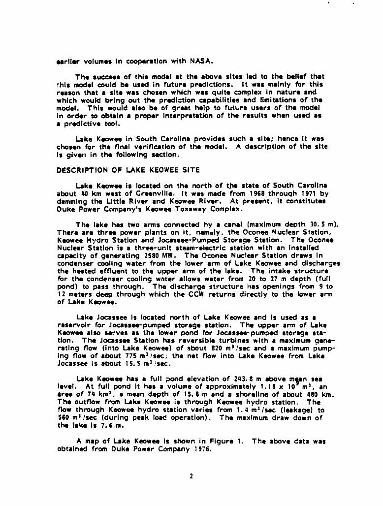
earlier volumes in cooperation with NASA.
The success of this model at the above sites led to the belief thatthis model could be used in future predictions. It was mainly for thisreason that a site was chosen which was quite complex in nature andwhich would bring out the prediction capabilities and limitations of themodel. This would also be of great help to future users of the modelIn order to obtain a proper interpretation of the results when used asa predictive tool.
Lake Keowee in South Carolina provides such a site; hence it waschosen for the final verification of the model. A description of the siteIs given In the following section.
DESCRIPTION OF LAKE KEOWEE SITE
Lake Keowee is located on the north of the state of South Carolinaabout 40 km west of Greenville. it was made from 1%8 throuqh 1971 bydamming the Little River and Keowee River. At present, it constitutesDuke Power Company's Keowee Toxaway Complex.
The lake has two arms connected by a canal (maximum depth 30.5 m).There are three power plants on it, namely, the Oconee Nuclear Station,Keowee Hydro Station and Jocassee-Pumped Storage Station. The OconeeNuclear Station is a three-unit steam-eiectric station with an installedcapacity of generating 2580 MW. The Oconee Nuclear Station draws incondenser cooling water from the lower arm of Lake Keowee and dischargesthe heated effluent to the upper arm of the lake. The intake structurefor the condenser cooling water allows water from 20 to 27 m depth (fullpond) to pass through. The discharge structure has openings from 9 to12 meters deep through which the CCW returns directly to the lower armof Lake Keowee.
Lake Jocassee is located north of Lake Keowee and Is used as areservoir for Jocassee-pumped storage station. The upper arm of LakeKeowee also serves as the lower pond for Jocassee-pumped storage sta-tion. The Jocassee Station has reversible turbines with a maximum gene-rating flow (into Lake Keowee) of about 820 m 3 /sec and a maximum pump-ing flow of about 775 m 3 /sec; the net flow into Lake Keowee from LakeJocassee is about 15. 5 m 3 /sec.
Lake Keowee has a Ball pond elevation of 243.8 m above m1an sealevel. At full pond it has a volume of approximately 1.18 x 10 m 3 , anarea of 74 km 2 , a mean depth of 1S.8 m and a shoreline of about 480 km.The outflow from Lake Keowee Is through Keowee hydro station. Theflow through Keowee hydro station varies from 1. 4 m 3 /sec (leakage) to560 m 3 /sec (during peak load operation) . The maximum draw down ofthe lake is 7.6 m.
A map of Lake Keowee is shown in Figure 1. The above data wasobtained from Duke Power Company 1976.
2
SECTION 2
CONCLUSIONS
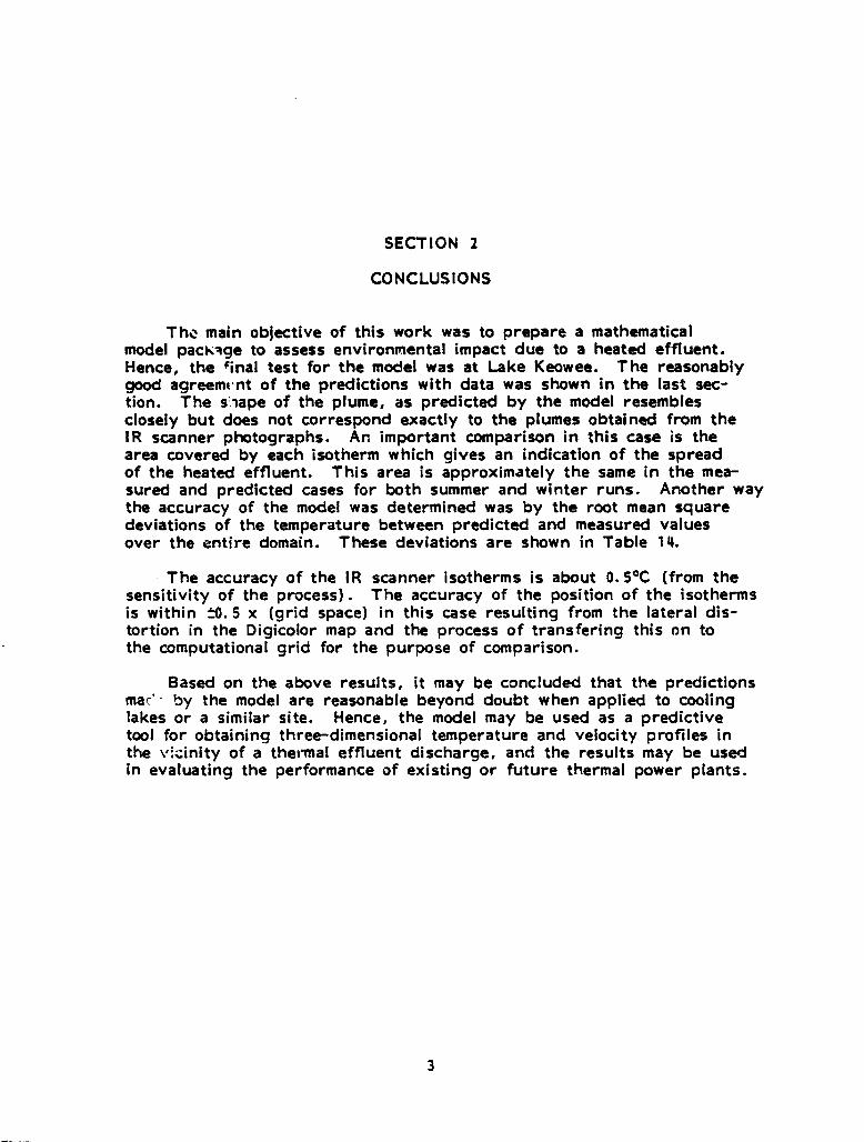
The main objective of this work was to prepare a mathematicalmodel pace:-ige to assess environmental impact due to a heated effluent.Hence, the final test for the model was at Lake Keowee. The reasonablygood agreement of the predictions with data was shown in the last sec-tion. The slape of the plume, as predicted by the model resemblesclosely but does not correspond exactly to the plumes obtained from theIR scanner photographs. An important comparison in this case is thearea covered by each isotherm which gives an indication of the spreadof the heated effluent. This area is approximately the same in the mea-sured and predicted cases for both summer and winter runs. Another waythe accuracy of the model was determined was by the root mean squaredeviations of the temperature between predicted and measured valuesover the entire domain. These deviations are shown in Table 14.
The accuracy of the IR scanner isotherms is about 0.5°C (from thesensitivity of the process) . The accuracy of the position of the isothermsis within ±0.5 x (grid space) in this case resulting from the lateral dis-tortion in the Digicolor map and the process of transfering this on tothe computational grid for the purpose of comparison.
Based on the above results, it may be concluded that the predictionsmac'- by the model are reasonable beyond doubt when applied to coolinglakes or a similar site. Hence, the model may be used as a predictivetool for obtaining three-dimensional temperature and velocity profiles inthe v :.cinity of a thermal effluent discharge, and the results may be usedin evaluating the performance of existing or future thermal power plants.

SECTION 3
RECOMMENDATIONS
Various numerical models have been developed to study the effectsof heated discharge and meteorological conditions on bodies of water.Most of these models are one or two dimensional. These models have ahigh computational speed but only give horizontally or vertically averagedvalues of temperatures.
Three-dimensional models, however, have a much finer resolutionbut they consume larger computer time. The three-dimensional rigid-lid model can be used to obtain detailed temperature and velocity distri-butions in a domain where surface gravity waves are small compared tothe depth of the domain. This model, as compared to free-surface mo-dels, runs faster since surface gravity waves are eliminated by thisrigid-lid assumption.
A proper method of using this model would be to run a one-dimen-sional model initially to obtain a rough picture of the temperatures andthen using this model to obtain a better resolution, the 1-1) results beingused as ambient conditions.
The following improvements have been suggested for the model.
1. Since all natural flows are turbulent, proper turbulent closures areneeded to make the model meaningful. At present, the simplestpossible closures, namely constant eddy viscosities an= .-ddy diffu-sivities, have been used. However, better results may be obtainedby using a higher order closure.
2. At present, the model uses uniform horizontal grids and stretchedvertical grids. Nonuniform horizontal grids could be introduced forbetter resolution near the boundaries.
3. The program has been written to be run as a batch-job on the com-puter. It could be made interactive so as to enable the user to runit on a terminal. However, this would require some modifications inorder to reduce the storage space.
4

SECTION 4
MATHEMATICAL FORMULATION AND MODEL DESCRIPTION
CHOICE OF MODEL
Two three-dimensional models have been developed by the thermalpollution group at the University of Miami. The first one is a free-sur-face model, which takes into account the variation in surface heights ofa basin. The second one is the rigid-lid model which assumes the verti-cal velocities on the water surface as zero. These models have been de-scribed in previous publications of this group. The choice of a particularmodel for simulating flows depends on the nature of the site.
Lake Keowee is a relatively small, closed basin with maximum depthof 30 m. The small horizontal numerical grid dimensions demand extremelysmall integration time steps to satisfy the Cou rant- Lew y-Fredrichs condi-tions inherent in free-surface formulations. Since the surface waves aresmall compared to the depth, i.e. h/H«1, a rigid-lid formulation is suit-able: This rigid-lid model allows acceptable accuracy with acceptabletime step size since the C.L.F. criterion is eliminated. This makes therigid-lid model a rather obvious choice.
The rigid-lid model has been applied previously to Biscayne Bay andLake Belews sites with reasonable accuracy, as mentioned in the previoussection. This led to the belief that it would be ideally suited for theKeowee site.
DESCRIPTION OF THE MODEL
(Portions of the following section have been published earlier bythis group.)
The rigid-lid model has the following capabilities:
1. Predict the wind-driven circulation.
2. Predict the circulation caused by inflows and outflows to the domain.
3. Predict the thermal effects in the domain.
4. Combine the aforementioned processes.
The model solves equations for fluid flow (momentum and continuity)
5
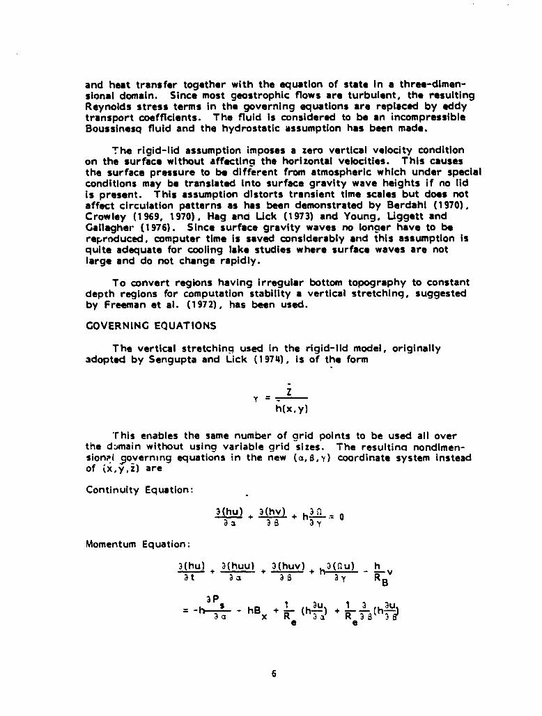
and heat transfer together with the equation of state in a three-dimen-sional domain. Since most geostrophic flows are turbulent, the resultingReynolds stress terms in the governing equations are replaced by eddytransport coefficients. The fluid is considered to be an incompressibleBoussinesq fluid and the hydrostatic assumption has been made.
The rigid-lid assumption imposes a zero vertical velocity conditionon the surface without affecting the horizontal velocities. This causesthe surface pressure to be different from atmospheric which under specialconditions may be translated into surface gravity wave heights if no lidis present. This assumption distorts transient time scales but does notaffect circulation patterns as has been demonstrated by Berdahl (1970),Crowley (1969, 1970) , Hag and Uck (1973) and Young. Liggett andGallagher (1976). Since surface gravity waves no longer have to bereproduced, computer time is saved considerably and this assumption isquite adequate for cooling lake studies where surface waves are notlarge and do not change rapidly.
To convert regions having irregular bottom topography to constantdepth regions for computation stability a vertical stretching, suggestedby Freeman et al. (1972) , has been used.
GOVERNING EQUATIONS
The vertical stretching used in the rigid-lid model, originallyadopted by Sengupta and Lick (1974) , is of the form
Zy = -
h(x, y)
'p his enables the same number of arid points to be used all overthe d;,main without using variable grid sizes. The resultin g nondimen-sion:l governing equations in the new (a,B,y) coordinate system insteadof jx,y,z) are
Continuity Equation:
3(hu) + 3(hv) + h33 k' = 0as a 3y
Momentum Equation:
3(hu) + a(huu) + 3(huv) + h 3(nu) _ h vat as as 3y RB
-t1-3 - hBx + R ( u) + R 3 B(h3u^
e e
6
w here a^' = at
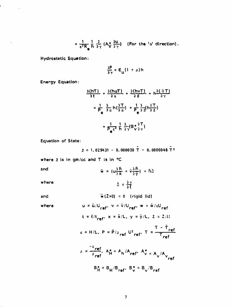
+ e^R h aaY (AV 3y ) (For the 'a' direction) .e
Hydrostatic Equation:
aP = E u (1 + p)h
Energy Equation:
a(hT) + a(huT) + a(hvT) + h a(s^T)at as as 3
_ 1 a aT + haT
Pe a`a h( aa) Pe aas a —a)
1 1 a * a + re E3 h 3y(Bvay)
Equation of State:
= 1. 029431 - 0. 000020 T - 0. 0000048 T 2
where 3 is in gm/cc and T is in °C
andw = (uT+v Y) +Fib
and 'w (2=0) = 0 (rigid lid)
w here u= u i U ref' v= v /U ref' w- w/ EU ref
t= t /tref' x= ill-, y = y /L, Z- Z it'
E= H/L, P= P/a U= T TTrefref ref' -
--y-r^
-pref
a - pref' A H - A h' ref' Av = Av/Avref
B H - BH /B ref' B - B By y ref
7
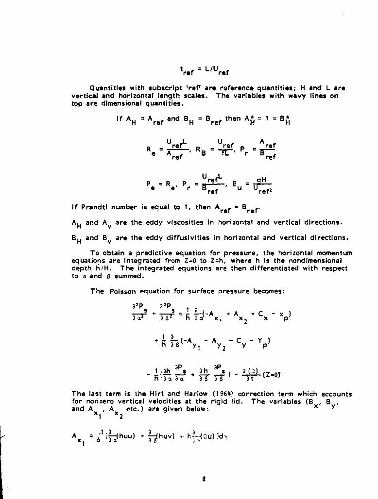
tref = LIU ref
Quantities with subscript 'ref are reference quantities; H and L arevertical and horizontal length scales. The variables with wavy lines ontop are dimensional quantities.
If AH = Aref and BH - Bref then AH = 1 = BH
R __ U refL R __ U ref P = Aref
e Aref B fl- r W—.
UrefL
=tfPe = Re, Pr = refEu _z
If Prandtl number Is equal to 1, then A ref = Bref'
A H and A are the eddy viscosities in horizontal and vertical directions.
B and By are the eddy diffusivities in horizontal and vertical directions.
To obtain a predictive equation for pressure, the horizontal momentumequations are integrated from Z =0 to Z=h, where h is the nondimensionaldepth h/H. The integrated equations are then differentiated with respectto a and 6 summed.
The Poisson equation for surface pressure becomes:
a^ + a ePID
= h 3-{-A X, + Ax + C - xp)2
+ h 3 g (-A y - A y + C y - Yp)
1 2
aP aPI 3h
- F { aa as + as a 8 } a3t) (Z=oi
The last term is the Hirt and Harlow (1964) correction term which accountsfor nonzero vertical velocities at the rigid lid. The variables (B X 0 By,and A , A etc.) are given below:
x 1 x2
Ax = 81 { 3,--athuu) + -:,Ihuv) • h.' {2u) )dYi
8

A = R 61 vdyx2 B
C _ 1 r1 { 3 (h au ) + 3 (h a uj + 1 1 3 tA* a u ) Yx Re O 3a as 38 3s ¢ aY v a y
Xp = E11 h{3h oYody + has oyp dy - Y 3a P}dY
Ay = 01 {a huv) + -as-a(huv + ah aYv))dY1
A = h I1 ud Yy2 RB o
1 1 3 a 3 au 1 1 3 ^3uCy = Re u { a ha- + a—{a h aB ) + T h 3Y (AvaY) }dY
Yp = E u f h {38 ryod-, + 0- pfypd - Y 38p )dy
Bx u= E h ^.Ypdy + EuhaB fY adY - EuY e0
The set of equations (24-30) together with appropriate boundaryconditions constitute the mathematical model. The model has been de-scribed in earlier publications by this qroup (Lee and Sengup ta, 1976).
INITIAL AND BOUNDARY CONDITIONS
The nature of the equations requires initial and boundary conditionsto be specified. As the ;nitial condition, the velocities, temperaturesand densities are specified throughout the domain. Boundary conditionsare specified at the air-water interface, geographical boundaries of thedomain, the bottom of the basin and the efflux points. At the air-waterinterface a wind stress and a heat transfer coefficient are specified.The conditions on the lateral wads are no-slip and no-normal velocityfor the momentum equations. These wails are assumed to be adiabatic.At the floor of the basin, the conditions of no-slip and no-normal velo-cities are applicable. The energy equation has a heat flux boundarycondition.
At points of efflux open-boundary conditions are specified. If theflows are known at the points of efflux, the flow velocities are specified.Usually, the temperature is known only at the point where the heateddischarge (from the power plant) enters the domain. At points wherethe temperatures are not explicitly known, open-boundary condition (i.e.zero gradient condition) is specified. The same holds true if the velo-cities are not explicitly known (e.g. the connecting canal between the
9
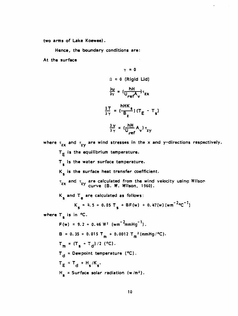
two arms of Lake Koewee) .
Hence, the boundary conditions are:
At the surface
Y = 0
R = 0 (Rigid Lid)
au hHay = (U re v Tzx
hHKaY = (-g-1 ) (T E - Ts)
z
av hHA )T
aYY - U ref v zy
where TzX and Tzy are wind stresses in the x and y-directions respectively.
T is the equilibrium temperature.
T s is the water surface temperature.
K is the surface heat transfer coefficient.s
TZx and zt are calculated from the wind velocity using Wiisor
y curve (B. W. Wilson, 1960).
K and T are calculated as follows:s e
K s = 4. 5 + 0.05 T s + BF(w) + 0.47(w) (wm-20C-1)
where T is in °C.s
F(w) = 9.2 + 0.46 W 2 (wm-2 mmHg- 1).
B = 0. 35 + 0.015 T + 0.0012 Tm2 (mmHg /°C).
T = (T s + Td ) /2 (°C) .
T d = Dewpoint temperature (°C
T = Td + H s /Ks.
H s = Surface solar radiation (w /m 2 ) .
10

At the bottom of the basin
1
On lateral walls
Y = I
n = 0
U = 0
V = 0
aT = 0ay
u - 0
v = 0
Sl = 0
aTax
aT _- as
Y ahh as
aT = 0ay
aTay =
aTas -
y ahFiaaay
aT = 0
SPATIAL DIFFERENCE SCHEMES
The numerical solution of the momentum and energy equations areexplicit. The values of velocities and temperatures at a future time aredetermined completely using the values at the present and previoustime steps. Finite difference forward time and central space differenceschemes are used. Diffusion terms are written using a Dufort-Frankelfinite difference scheme to relax the diffusive stability criterion. Theconvective stability criterion, however, is not affected.
A horizontal staggering is used in the computational grids. Hori-zontal velocities and temperatures are calculated at the main-grid pointswhile vertical velocities and pressures are calculated at half-grid points
The predictive Poisson equations for calculating rigid-lid pressuresis finite differenced using a five-point scheme. This is solved bysuccessive over relaxation (Liebmann Method) . Terms on the ri ght handside of the pressure equation are obtained b-., integrating terms in thehorizontal momentum equations over the depth using the trapezoidal rule.
At the boundaries, single-sided schemes are used since the boundarypoints do not have two adjacent points. A curve is fitted throu g h the
11
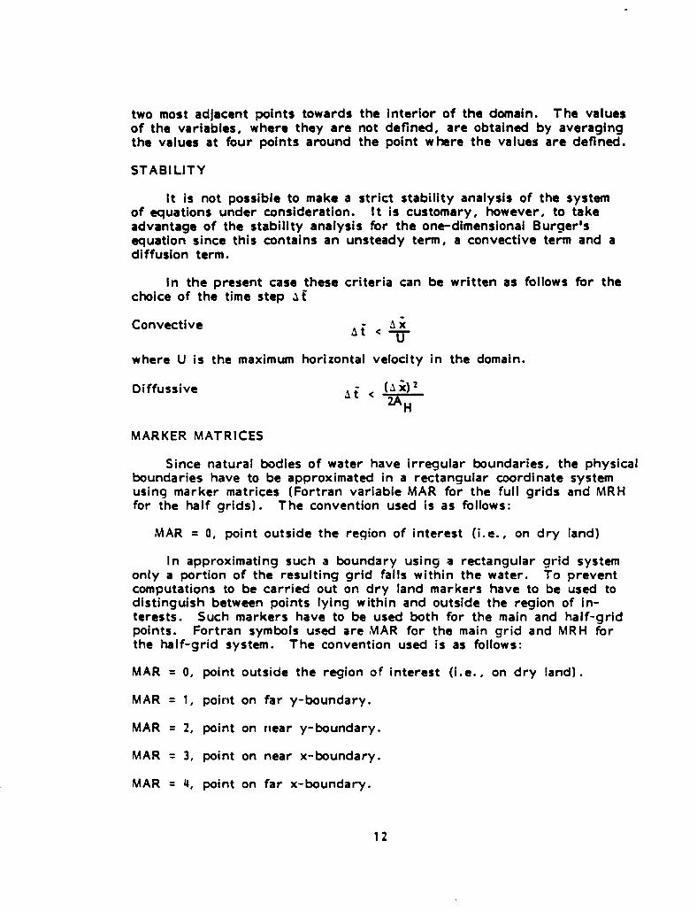
two most adjacent points towards the interior of the domain. The valuesof the variables, where they are not defined, are obtained by averagingthe values at four points around the point where the values are defined.
STABILITY
It is not possible to make a strict stability analysis of the systemof equations under consideration. It is customary, however, to takeadvantage of the stability analysis for the one-dimensional Burger'sequation since this contains an unsteady term, a convective term and adiffusion term.
In the present case these criteria can be written as follows for thechoice of the time step a i
Convective Ai < ^I xU
where U is the maximum horizontal velocity in the domain.
Diffussive L (^
H
MARKER MATRICES
Since natural bodies of water have irregular boundaries, the physicalboundaries have to be approximated in a rectangular coordinate systemusing marker matrices (Fortran variable MAR for the full grids and MRHfor the half grids) . The convention used is as follows:
MAR = 0, point outside the region of interest (i.e., on dry land)
In approximating such a boundary using a rectangular arid systemonly a portion of the resulting grid falls within the water. To preventcomputations to be carried out on dry land markers have to be used todistinguish between points lying within and outside the region of in-terests. Such markers have to be used both for the main and half-gridpoints. Fortran symbols used are MAR for the main grid and MRH forthe half-grid system. The convention used is as follows:
MAR = 0, point outside the region of interest (i.e., on dry land) .
MAR = 1, point on far y-boundary.
MAR = 2, point on near y-boundary.
MAR = 3, point on near x-boundary.
MAR = 4, point on far x-boundary.
12
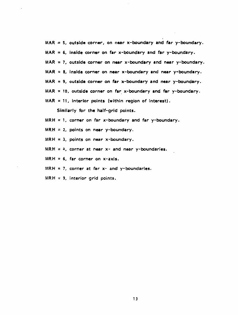
MAR = 5, outside corner, on near x-boundary and far y-boundary.
MAR = 6, inside corner on far x-boundary and far y-boundary.
MAR = 7, outside corner on near x-boundary and near y-boundary.
MAR = 8, inside corner on near x-boundary and near y-boundary.
MAR = 9, outside corner on far x-boundary and near y-boundary.
MAR = 10, outside corner on far x-boundary and far y-boundary.
MAR = 11, interior points (within region of interest.
Similarly for the half-grid points.
MRH = 1, corner on far x-boundary and far y-boundary.
MRH = 2, points on near y-boundary.
MRH = 3, points on near x-boundary.
MRH = u, corner at near x- and near y-boundaries.
MRH = 6, far corner on x-axis.
MRH = 7, corner at far x- and y-boundaries.
MRH = 9, interior grid points.
13
SECTION 5
APPLICATION TO LAKE KEOWEE
INTRODUCTION
The three-dimensional rigid-lid model described in Chapter II hasbeen applied to Lake Keowee, South Carolina, to predict the wind-drivencirculation, circulation caused by inflows and outflows, and the thermaldynamics of a region of this lake. This region includes the buoyantplume, the Keowee hydro dam, the connecting canal and an open-boun-dary where the effects cif inflow and outflow to Jocassee-pumped storagestation are felt.
Lake Keowee Is a warm monomictic lake having one circulation periodduring the year, beginning in fall, and is thermally stratified durinq thesummer. During the circulation period, the. water mass is verticallymixed. This type of lake can also be termed holomictic (Hutchinson,1957) . Lake Keowee could also be classified as a subtropical lake asit exhibits thermal stratification, a period of total circulation precededby the fall overturn, and surface temperatures above 4°C. The highestsurface temperatures typically occurred in July and August and rangedfrom approximately 27 to 29°C. During the periods from November t%,roughFebruary the lake was isothermal or nearly so. It can be concluded fromthe above that a series of meteorological events primarily govern LakeKeowee's thermal characteristic. However, as will be shown below, thenear field r gl'ao which makes up the region of interest in this presentstudy, is very strongly affected by the buoyant plume, inflow and out-flow and the Jocassee-pumped storage station.
CHOICE OF DOMAIN AND GRID SYSTEM
The region of interest has already been mentioned in the last sec-tion. Here, an attempt will be made to justify this choice and then adescription of the grid system will be given.
The study and prediction of the thermal impact on the hydro-dyna-mics of Lake Keowee has been done in two main sections:
1. Using a 1-D continuous temperature profile prediction model overthe period 1971-1979, the area of interest includes the two mainarms of Lake Keowee and the connecting canal. The application ofthis model has been published by the thermal pollution group of theUniversity of Miami (Sengupta et al 1980) .
14
2. Using the 3-D rigid-lid model, which is described In this report.
The division has been necessary since the 1-1) model predictstemperature profiles continuously over a period of time (several yearsIf required) ; it can be used to predict the initial conditions required torun the 3-D model. The 3-D model, on the other hand, has betterresolution and Is therefore used for predicting the near-field thermalImpact on the lake. This near-field area of interest is shown in FiqureS. In selecting this area some preliminary runs were made. These arer1o:scribed later.
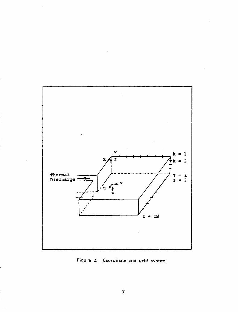
The region of interest is divided into a square grid as shown inFigure S. The I and J axes (corresponding to u and v-velocity axes)are numbered as shown In the above figure. For the top 'open boundary','J' increases from 7 to 20. The left side boundary shown 'I' increasingfrom 1 to 17; the right side boundary shows 'I' increasing from 1 to 16,and finally, the bottom boundary shows 'J' increasinq from 1 to 18. Theorientation of these boundaries with the north-south direction is alsoshown in this figure. The squares are (152.4 x 1S2.4) square meters.Arrows indicate directions of flow into or out of domain.
SUMMARY OF DATA
For the purposes of calibrating and verifying the model, an archivaldata base was established and two remote sensing and field data collectionmissions (summer and winter) were undertaken.
Archival Data Base
The archival data base are summarized in Figure 6 and Tables 1through 4. These figures were taken from Duke Power Company (1976).Figure 6 shows the measured surface isotherms for September 10, 1975.This figure constitutes the data base on which the comparisons for thepreliminary and archival runs are based. The runs are described below.Table 1 shows the monthly gross thermal capacity factors for OconeeNuclear Station (1973-1977). Table 2 is a summary of Oconee NuclearPower Plant fcr September 10, 1975. Table 3 shows the input dataused for the preliminary and archival runs. The data include the flow-rate, inlet temperature, discharge temperature and velocity, ambienttemperature, depth at discharge, discharge width, air temperature,wind speeds and the vertic it and horizontal eddy diffusivities. Table 4is a summary of the volu-ne and area data for Lake Keowee.
August 1978 Data
To obtain an understanding of seasonal behavior of Lake Keowee,data was gathered both in summer and winter. This datr, was used toverify temperatures predicted by the model. Two extreme weatherconditions were selected with the idea that if the model predictions wereaccurate for these conditions it would be so for other intermediate con-
15
ditions (viz., spring or fall) .
In spite of the fact that the model was used for predictions in thevicinity of the thermal plume, temperature and velocity readings weretaken for the entire lake. This was done in order to ensure complete-ness of the data and also to check the choice of the domain of interestwithin the lake.
Summer data missions were carried out during the period of August24 and 25, 1978. The data collection team consisted of representativesfrom NASA, EPA, University of Miami and Duke Power Company. Threeboats provided by Duke Power Company were used in the collection ofground truth data. The data collsction stations are shown in Figure 7.This included measurements of water temperatures at various depths(from the surface to about 30 m) using YSI type thermistors and velocitymeasurements using an Endeco Type 110 current meter. The thermistorswere calibrated before each set of readings using a mercury thermometer.At each measuring station the boat was anchored and the thermistorsand velocity meters were lowered by cables. The cables were markedthus indicating the depth below the water surface where readings weretaken. The current meter indicated both the magnitude and directionof the horizontal component of the water velocity. The main problemencountered here was that most of the velocities were very small andclose to the threshold of the instrument. Hence, drogues were used todetermine average surface velocities.
While the ground truth data was being collected, overflights weremade by NASA aircraft to obtain synoptic IR scanner data. The aircraft,a twin encined (Beechcraft) (NASA-6) , was specially equipped for thispurpose. Flights were made at altitudes of 1000, 2000 and 3000 ft. Adiagram of the flight plan is shown in Figure 8, The scanner photo-graphs were taken with window settings between 78 and 84°F. To cor-rect the IR scanner photographs with the ground truth data for eachset of flights, the water surface temperature was measured with theaircraft overhead for at least one station. This was to correct the scan-ner readings due to errors caused by water vapor attenuation.
The scanner used was a daedalus series DS-1250 and remote sensingof 8-14 ;,m radiation is achieved by a Hg: Cd: detector. The detectorhad a 0.015 inch square sensitive area, which was optimum for the reso-lution and temperature sensitivity requ;red- This detector was mountedIn an end-looking, metal cored cewar which had sufficient liquid nitrogencoolant capacity for approximately six hours of operation before refilling.Thi= :-ystem prciected through the floor of the airplane, NASA 6, andhad a «an angle of 120° centered above the vertical. A horizontally-mounted telescope with its axis along the direction of flight of the air-plane was contained within the scanner. A mirror rotating at 3600 RPMand mounted at 45 0 to the telescope directed heat radiation from theground into the system. A ore-third revolution of the mirror covered acomplete step perpendicular to the scanner axis. Optical resolution
16

obtained by this method was about 1.7 milliradians, so the ground areasdetected become a function of flight altitude; the data accuracy is 0. VC.
The video siqnal from the infrared detector was amplified and re-corded on magnetic tape in the aircraft. A method developed by Daedaluscalled Digicolor was used to convert this stored information directly intocolor coded strip imagery. This process limits the number of outputcolors to light (from white 'hottest' to black 'coldest') for any input con-dition. The six colors between white and black i..:iicate the six calibratedlevels of the set of interest. The scanner's thermal rzss-ante sourceswere present in flight to 66°F and 84°F respectively, and the settingswere recorded on the same track with the detector video to insure accu-rate voltage relationships irrespective of all amplifier gain adjustments.
The color bands in the final Digicolor map indicate zones of con-stant temperature within the accuracy of resolution of the scanner; hence,the line formed by the junction of two adjacent color bands indicate anisotherm. The actual temperature of the isotherm is obtained by addinga ground truth correction term to the temperature indicated in the map.
Altogether, three IR flights were made during the summer datacollection mission. Out of these, two runs were made on August 24.The first run was from 0853 hrs EST. On August 25, a single run wasmade from 0908 hrs to 0953 hrs EST.
The Digicolor maps were transfered on to enlarged maps of the regionof interest so as to obtain a map of surface isotherms which could be com-pared directly with the values predicted by the model. Out of the threeruns made, only two, namely August 24 morning and August 25 morning,were used for comparisons since the resolution of the colors in the re-maining Digicolor map was very poor.
The values of Oconee Nuclear Stations flows and temperatures everyhour are obtained from continuous water quality monitoring stations ofDuke Power Company. Flow through Jocassee-pumped storage stationand Keowee Hydro Station as well as meteorological conditions (viz., airtemperature, wind speed and direction, humidity and incident solar radi-ation; were also obtained from continuous monitoring stations. The flowsthrough Jocasse, Keowee and Oconee as well as the discharge temperaturesare shown in Tables 5 and 6. The meteorological data (obtained hourly)are shown in Tables 7 and 8. Figures 9 and 10 show the hourly variationof Keowee Hydro Station flowrate on these two days. Figures 11 and 12show the same for Jocassee-pumped storage station.
February 1979 Data
The winter data mission was carried out during February 27, 28,1979. The same equipment were used in this mission. Three boatswere used to measure water temperatures and velocities up to a depth of30 m. Two of the boats were equipped with thermistors only and were
17

used to measure temperatures in both branches of Lake Keowee. Thethird boat carried the current meter as well as a thermistor. The stationswhere readings were taken are indicated in Figure 13. Station #13 wasused for ground truth correction of the IR scanner data. This point waschosen since it is virtually unaffected by the discharge, and the tempera-tures here remained fairly constant.
Ground truth measurements were taken from 0950 hrs to 1353 hrsEST and 1600 hrs to 1833 hrs EST on February 27. Due to technicalproblems with the aircraft (NASA-6) the IR flights were delayed andwere only from 1549 hrs to 1711 hrs EST on this date. The flight planwas identical to that used in the August data. mission. Black body set-tings of 38°F and 74°F were used and the flight altitudes were 2000,3000 and 1000 feet.
On Feburary 28, 1979 ground truth measurements using three boatswere taken from 0851 hrs to 1201 hrs EST and 1420 hrs to 1830 hrs EST.IR flights were run from 0850 hrs to 1002 hrs at altitudes of 2000 and3000 ft. The black body settings used were established by NASA. IRisotherms were constructed for the domain of interest at the Universityof Miami. Thew maps were used for verifying the results predicted bythe computer.
For obtaining meteorological data and flows through Oconee NuclearStation, Jocassee-pumped storage station and Keowee Hydro Station,continuous monitoring stations of Duke Power Company, were used.Since the velocities in the lake were found to be extremely small, drogueswere also used. The flows through the three power stations are shownin Tables 9 and 10. The data obtained was hourly and the variation ofthe flows through Jocassee and Keowee are shown in Figures 14 and 15and Figures 16 and 17 respectively. The meteorological data collected onFebruary 27 and 28 are shown in Tables 11 and 12 respectively.
The ground truth data collected during the summer and wintermissions are presented by Duke Power Company (1978 and 1979) .
CALCULATION OF INPUT
The 3-D rigid-lid model as described in Section 4 solves the three-dimensional momentum, continuity and energy equations. As shown be-fore, these equations are a set of nonlinear, coupled partial differentialequations and require the following for complete solution.
1. Initial values of the velocities and temperatures must he specifiedat all points within the domain.
2. Boundary conditions for the above variables must be specified atall boundaries.
The choice of the domain of interest as well as the grid system has
18

been described in earlier sections. At all solid boundaries the velocitiesand temperature gradients are specified as zero. At the surface therigid-lid constrain. of zero vertical velocities is assumed. The initialconditions assumed for starting the runs are zero velocities and con-stant temperatures everywhere within the domain. For subsequent runsthe results of the previous run is used as the initial condition. Hence,the quantities yet to be specified are:
1. Temperatures and flow velocities at the Oconee Nuclear Station dis-charge.
2. Temperatures and velocities at the Keowee Hydro Station.
3. The same at the Jocassee boundary and at the canal. (items 1 and 2).
4. Surface horizontal velocities and temperatures.
The above quantities are termed as inputs to the model and theprocedure used for obtaining them are discussed briefly below for thesake of completeness. For further details regarding the actual runningof the prugrams, the reader is_ advised to refer to the 3-D riqid-lidUser's Manual (Sengupta et al, 1980) prepared for this purpose.The calculations shown below were for February 27, 1979 simulations.
Reference Quantities Used
Reference length = L = maximum length of the domain = 2895.6 m.
Reference horizontal eddy viscosity A ref = 0.002 L 4/3 = 38311.48 cm /sec.
(Note: The constant 1 0.002' changes with different sites. This particu-lar value was used in running the model at Lake Belews and at BiscayneBay. In this case the best value of the constant was found to be '.003'which yielded a value of Aref = 60,000 cm /sec.
Reference depth = H = max depth considered = 16 m
Reference vertical eddy viscosity A V = 0. 002 x H 413 = 37. 43 cm 2 /sec.
Reference velocity U ref = 30 cm /sec.
Reference time T ref = L/V ref = 9652 sec.
Oconee Nuclear Station Discharge Velocity
The discharge is considered to take place through a point at a depthof 12 m (k=3) . The discharge velocity is calculated as follows.
19

12 m .4rV
152. 4 m
The total discharge = (100 m x V( m ) x 152.4 x 12) = Qsec
(where Q = average discharge In m 3 /sec . )
. ' . V = 7. 4207 cm /sec
The average value of 'Q' over 24 hrs is taken since the variationis negligible.
Nondimensional discharge velocity= V-V = V = 0.24740.ref
Keowee Hydro Discharge Velocity
The outflow through the Keowee hydra station is through a channel(152.4 m) x (12 m).
The volume flowrate Q = 0 52. 4 x 12 x V) m ; /sec.
(where V = discharge velocity (m /sec. )
V = [Q / 0 52. 4 x 12)) m /sec = Q52. 4x 12x 100 cm /sec
Q is specified as a function of time with the help of polynomials andother functions. The curve is approximated and specified in subrou-tine INLETI; (refer to the user's manual (Sengupta et al, 1980).
Keowee hydro flow approximation: refer to the user's manual (Senoupta et al,1980) .
(February 27 Data)
SX = Conversion factor for converting discharge (incfs) to nondimensionalvelocity.
SV 1 = Nondimensional velocity.
The velocities are approximated as follows:
SV 1 = 0.048 0 < TSDT < 6
20
SV 1 = SX * (((17.54 - 0.048) J 2.) * (TSDT - 6.0) + 0.48)
6 < TSDT < 8
SV 1 = SC * (((.048 - 17.54) /4.) * (TSDT - 8.0) + 17.54)
8 < TSDT < 12
SV 1 = SX * (0.048) 12 < TSCT < 24
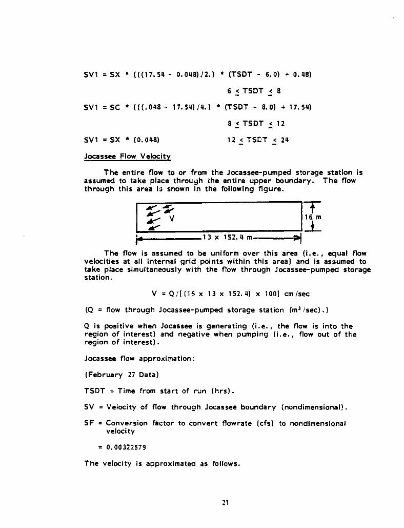
Jocassee Flow Velocity
The entire flow to or from the Jocassee-pumped storage station isassumed to take place through the entire upper boundary. The flowthrough this area is shown in the following figure.
.r
Il 16. m
.13 x 152. 4 m--_^
The flow is assumed to be uniform over this area (i.e., equal flowvelocities at all internal grid points within this area) and is assumed totake place simultaneously with the flow through Jocassee-pumped storagestation.
V = Q !( (15 x 13 x 152. 4) x 1001 cm /sec
(Q = flow through Jocassee-pumped storage station (m' /sec) . )
Q is positive when Jocassee is generating (i.e. , the flow is into theregion of interest) and negative when pumping (i.e., flow out of theregion of interest) .
Jocassee flow approximation:
(February 27 Data)
TSDT = Time from start of run (hrs) .
SV = Velocity of flow through Jocassee boundary (nondimensional) .
SF = Conversion factor to convert flowrate (cfs) to nondimensionalvelocity
= 0.00322579
The velocity is approximated as follows.
21
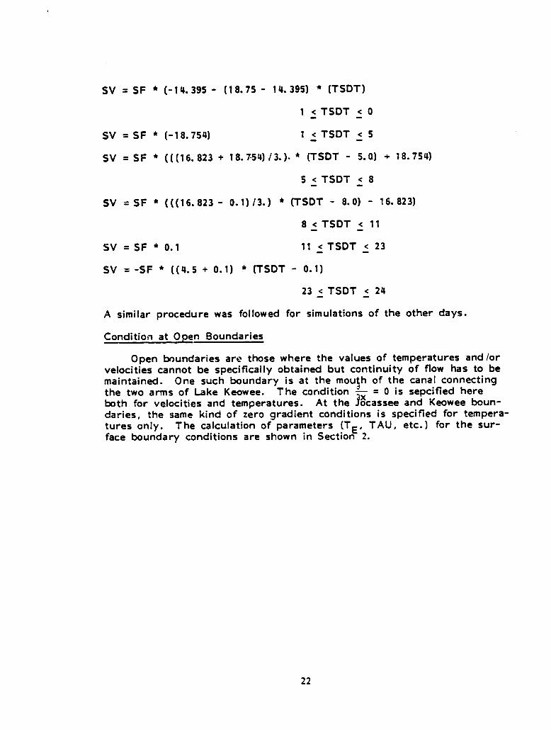
SV = SF * (-14.395 - (18.75 - 14.395) * (TSDT)
1 < TSDT < 0
SV = SF * (-18.754) 1 < TSDT < 5
SV = SF * M16.823 + 18.7-54)11).). * (TSDT - 5.0) + 18.754)
5 < TSDT < 8
SV = SF * (( ( 16.823 - 0.1) 13.) * (TSDT - 8.0) - 16.823)
8 < TSDT < 11
SV = SF * 0.1 11 < TSDT < 23
SV = -SF * ((4.5 + 0.1) * (TSDT - 0.1)
23 < TSDT < 24
A similar procedure was followed for simulations of the other days.
Condition at Open Boundaries
Open boundaries are those where the values of temperatures and/orvelocities cannot be specifically obtained but continuity of flow has to bemaintained. One such boundary is at the mouP of the canal connectingthe two arms of lake Keowee. The condition = 0 is sepcified hereboth for velocities and temperatures. At the Iocassee and Keowee boun-daries, the same kind of zero gradient conditions is specified for tempera-tures only. The calculation of parameters (T E , TAU, etc.) for the sur-face boundary conditions are shown in Section 2.
22
L
SECTION 6
RESULTS AND DISCUSSIONS
The results of simulation using the 3-D rigid model at Lake Belewsand Biscayne Bay are shown in previous publications by the Universityof Miami (Lee, Sengupta and Mathavan, 1977, end Lee and Sengupta,1976) . In the above two cases the predictions made by the model agreedclosely with IR scanner and ground truth data. The following sectiondiscusses the runs made for Lake Keowee.
Preliminary Runs and Results
These runs were primarily made for the selection of the boundar,conditions, initial conditions and to test the behavior of the model whenincomplete and/or arbitrary data are used. These runs are summarizedin Table 13.
1. Run Number L001
(The Number L001 is a sequence number and must only be interpretedas such.)
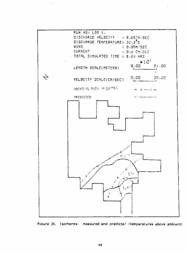
This run was essentially made for debugging the computer programmodifications. The features include a discharge velocity of 5.65 cm/sec, a discharge temperature of 32.3°C and a 16 meter constant depthregion of interest. The total simulated time was 20.6 hours. Theresults are summarized in Figures 18, 19 and 20. The surfacevelocities after 8.64 hours are shown in Figure 18, while Figure 19shows the velocities in a vertical plant (1=11) after 21.6 hours.Since the effects of wind were not included in this run and therewere no effects of Jocassee, the velocities are by the dischargevelocity and the buoyant plume. The isotherm comparison of thearchival run and this simulation run is shown in Figure 20. Theambient temperature is 29°C. The archival isotherms are higherthan the predicted isotherms. This is expected since this run(without wind) was not undertaken primarily for comparison pur-poses, and the simulation did not reach st;"&-dy state.
2. Run Number L002
This run is similar to 'L001' but with variable depth of the regionof interest. The simulation time was only 8.64 hrs. This time islong enough to determine how well the model hndles a variably:
23
depth domain. The surface velocities and vertical velocities (at1=11) are shown respectively in Fiqures 21 and 22. For complete-ness, the simulated surface isotherms are compared with the archivalIsotherms. This comparison is shown in Figures 23. For the same'reason described in the previous subsection, the comparison cannotbe expected to be more precise.
3. Run Number L003
Run L002 is now repeated with the effects of wind included. Thetotal time simulated was only 8.00 hrs. The reason far the shortsimulation time is as explained above . The surface andvertical velocities (J=7) are shown in Figures 24 and 25 respectively.A comparison of Figures 21 and 24 shows the small effects of wind onthe surface velocities after such a small simulation time. The windspeed is 4 m / sec. A comparison of the predicted and archival iso-therms is shown in Figure 26. Compared with the other isothermcomparisons, this figure appears to have improved the difference be-tween measured and predicted.
Archival Runs and Results
Two runs were made (L004 and L005) using the archival data basedescribed in the last section.
1. Boundary Conditions
The following specifications were used at the main input boundaries.
a. At 1=1, J=8 to 19 for all depths (K)
The water velocity at the Jocassee end is specified as 6. 9 cm /sec. Open boundary is specified for temperatures as this end.
b. At 1=11, J=1, K=3
This discharge velocity is specified as 5.65 cm /sec, and thedishharge temperature also specified as 32.4°C.
c. Finally, at 1=13, J=7, K=1 to 3
Keowee dam discharge velocity is specified as 10. 4 cm /sec.
2. Run Number L004
This k°,. the first archival run and was made with variable depthtopog , aphy for the near-field region of interest.
3. Run Plumber L005
24
I
Run L004 is repeated but for constant depth region of interest.The domain was cut off at 16 meters from the water surface. Thisis the depth of the thermocline for Lake Keowee.
4. Archival Results
Figure 27 shows the comparison between the measured (archival9/10/75) and calculated (LO04) isotherms. The ambient temperaturewas 29°C. This comparison can be seen to have improved whencompared to those of the preliminary runs already described. Thesurface velocities are similar !o 'LOOS' which are shown in Figure 28.Flow through the Keowee drat can be seen very clearly on the rightboundary of the figure. Figure 29 shaves the velocity field at J=7,which also shows the flow through the Keowee dam. The isothermcomparisons of measure.! (9/10/75) and predicted (LOOS) is shownin Figure 30. This is the best comparison of the runs described sofar. The agreement is particularly good for the 29.5 and 30*C iso-therms. The shapes of the measured and predicted 30.5°C isothermsare similar. However, the measured area under the isotherm appearsbigger. This discrepancy can be explained in terms of the nearnessof this isotherm to the discharge. The total time simulated was 32.4hrs, which is also the time when steady state was reached. Thetemperature profiles for locations 1=11, J=7, K=1 to 4 through thesimulated period are shown in Figure 31. The temperature profilesare vertical as expected since computations were carried out abovethe thermocline. A comparison of the surface velocities at this loca-tion is given in Figures 32. It can be seen from this figure that theu-component velocities predominate. It can also be seen from thisfigure that all the velocities stabilize after about 30 hours, showingsteady state conditions. A similar plot, Figure 33, for the samevariables but for location 1=11, J=2 and K =1 is shown. Similar con-clusions hold for this figure.
L001 through L005 were archi ral runs. The following section dis-cusses the results of simulations for the August data base (LO06)and February data base (LO07) . Both these runs were made instabs of 24 hrs of simulation at a time for a total period of 48 hoursof simulation in each case. Results were stored and printed at theend of every hour of real time. The results at the end of the first24 hrs simulation were used as initial conditions for the next 24 hrs.
Summer Runs
Simulation was started from 0000 hrs August 24. The model wasstarted 'cold' i.e., initial conditions used were zero velocities and con-stant temperature (29°C) throughout the domain. This conditions re-quired that the model had to be run for sometime before the effects ofthe cold start could be ignored.
The inputs used in running the model have been discussed in the
25
previous section. The wind speed driving the upper layer varied from0.76 to 3.09 m /sec. The current or the flow through the Jocasseeboundary varied from 0.61 to 1.12 cm /sec. The Oconee nuclear stationdischarge velocities and temperature were 7.42 cm /sec and 31.7°C re-spectively. (Average values were taken since the fluctuation was negli-gible.) All the above data were fed in every hour in running the model.
The surface isotherms and velocities at each horizontal section(K=1, 2, 3, 4 and 5) were plotted using a Calcomp plotter. Results atthe end of each hour were stored and plotted. The results used forcomparison were the surface isotherms plots. Measured surface isothermswere obtained from IR scanner digicolor maps. By drawing both thedata and the predicted values on the same grid system direct comparisoncould be made.
The first IR runs were made on August 24 from 0853 hrs EST to1002 hrs EST. The Isotherms drawn for this data are shown in Figure34. The isotherms shown are for 30.5°C, 30.0°C and 29. S°C. Only theabove three isotherms fell within the domain of interest and representthe water surface temperatures at 1002 hrs EST, August 24, 1978. Theresults produced by the model are shown in Figure 3S and 36. Figure 3Sshows the same isotherm i.e., 30.5°C, 30.0°C and 29.5°C correspondingto 1007 hrs real time. It is seen that the temperatures predicted by themodel are lower than the actual temperatures, showing that the plumespread was underpredicted. Figure 36 shows different predicted iso-therms corresponding to the same time. The temperatures of the iso-therms are 29.50C, 29.3°C and 29.1 °C. Comparing Figure 36 with 34it is seen that 29.5 0C in the IR data a grees very well with the 29.1 °Cisotherm predicted by the model. The measured 30.5°C and 30.0°C iso-therms compared with the predicted 29.5°C and 29. 3°C isotherms respec-tively. Hence, the errors in prediction in the three isotherms (30. 5°C ,30.0°C and 29.5°C measured) are approximately 1°C, 0.7°C and 0.4°Crespectively.
The IR digicolor map for the August 24 afternoon data could not beused to construct isotherms because of bad resolution between differentcolors. Hence, the next useful comparison was made for the August 25morning data (0903-9553 hrs EST). The IR isotherms are shown inFigure 37. The same three temperatures, namely 30.5°C, 30.0°C and29.5°C, are represented here since the other isotherms lie beyond thedomain of interest. Figure 38 shows the same isotherms as predicted bythe model. The spread of the 29.5°C isotherm is overpredicted whilethe 30.0°C isotherm is underpredicted. However, Figure 39 shows iso-therms for 29.90°C, 29.70°C and 29.6°C as predicted by the model.These isotherms compare very well with the IR isotherms in Figure 37.The errors in this case are .6°C for the 30.5°C isotherm, 0.3°C forthe 30.0°C isotherm and -.1 0C for the 29. 5°C isotherm. This shows aconsiderable improvement in the predictions as compared to August 24,showing the effects of cold start gradually vanishing.
26
Figure 40 shows the plot of the horizontal velocities of the surfaceas predicted by the model for 1007 hrs, August 24. During this time(1007 hrs EST), as can be seen from the Jocassee-pumped storage sta-tion flow and Keowee hydro station flow data, the flows through thesestations were negligible. This leads to zero velocities at Jocassee boun-dary and zero velocity through the Keowee hydro discharge point inFigure 40.
Figure 41 shows the surface horizontal velocities predicted by themodel for August 2S ( 33.2 hrs run time) . During this time (approxi-mately 1000 hrs, August 25) Jocassee-pumped storage station just startedgenerating and Keowee hydro was generating. This accounts for the flowsthrough the two boundaries.
The main driving forces responsible for determining the shape ofthe isotherms are the ambient temperature, discharge temperature andflows through the Jocassee boundary. The wind is seen to affect thevelocities in the upper layer only. This characteristic is displayedboth in the data and the simulation results, Figure 34 (August 24 IRdata) and Figure 37 (August 24 IR data) . Looking at the Jocassee andKeowee flows it is seen that the flow through Jocassee is negligible dur-ing both these periods. The flow through Keowee is negligible at 10.00a.m. on August 24 but is 9352 cfs on 10 a.m., August 25. The averagedischarge temperature is also lower on August 25 as compared to August24. This causes the area under the isotherms in Figure 37 to be lowerthan those in Figure 34. The same difference is seen between the cor-responding predicted isotherms, namely Figure 36 (August 24, 1978) andFigure 39 (August 25) .
Winter Runs
Simulation was started from (0000 hrs) February 24, 1979. Themodel was started using zero velocities and constant temperature (= 10°C)as initial conditions.
The inputs used for this run (1-007) have been discussed in detailIn previous sections. The Oconee discharge velocity (average value) was6.84 cm /sec and the discharge temperature (average value) was 18. 4°C.The wind speed varied from 1.61 to 4.52 m /sec and the Jocassee-pumpedstorage station boundary flow velocity ranged from 0.61 to 4.14 cm /sec.
Values of velocities and temperatures were printed at the end ofevery hour. Surface isotherm plots and velocity plots were generatedfrom these results. Figure 42 shows the IR scanner isotherms for 1648-1651 hrs, February 27. The temperatures are 13.0°C, 12.5°C, 12.0°C,11.5°C and 11.0°C. The same isotherms as predicted by the model areshown in Figure 43. Thr= p correspond to 17.12 hrs after the coldstart. Comparing these two figures it is seen that the isotherms pre-dicted by the model have a greater spread. Figure 44 shows predictedisotherms corresponding to 13.75°C, 13.0°C, 12.75°C, 12.5°C and 12.0°C.
27
This figure agrees better with Figure 42 showing an error of predictionof 0.75°C, 0. VC, 0.75°C and 1 °C respectively for each of the isotherms.
Figure 45 shows IR scanner isotherms for February 28, 1979 corre-sponding to 0948-0957 hrs EFT. The two Isotherms within the domainare for 13.0°C and 12. S°C. Figure 46 shows the same two isotherms aspredicted by the model. These correspond to 34.2 hrs of run time afterthe cold start at approximately 10 a.m., February 28. Figure 46 is inexcellent agreement with Figure 45. Isotherms for IR data correspondingto February 28 afternoon could not be drawn because of bad resolutionamong different colors In the digicolor map.
Figure 47 shows velocities at the surface as predicted by the modelfor February 27, 17.12 hrs after the cold start. The flows through theJocassee and Keowee hydro boundaries agree with the data obtained.Figure 48 shows the same for February 28, 34.2 hrs after cold start.Excellent agreement is obtained in this case between the velocities shownon the map and measured flows at Keowee hydro station and Jocassee-pumped storage station. As in one of the summer runs, the isothermsare affected by the Oconee discharge, Keowee hydro and J ocas see- pumpedstorage station. Figures 42 and 45 (isotherms for February 27 and 28respectively) show that the isotherms have spread out further on thesecond date. Keowee hydro and Jocassee-pumped storage station flowsare negligible on both the dates. The average Oconee discharge tempera-ture during 1600 hrs, February 27, was lower than that durinq 1000 hrs,February 28. This accounts for the greater spread of the isotherms.The same is depicted in the results produced by the model.
28

REFERENCES
Duke Power Company. Oconee Nuclear Station Thermal Plume Study.1978.
Duke Power Company. Oconee Nuclear Station Thermal Plume Study.1979.
Duke Power Company. Oconee Nuclear Station Environmental SummaryReport, 1971-1976. 1976.
Freeman, N. G., Hale, N. G. an-' M. B. Danard. A Modified SigmaEquations Approach to the Numerical Modelling of Great LakesHydrodynamics. J. Geo. Res., Vol. 77, No. 6. 1972.
Haq and W. Lick. The Time-Dependent Wind-Driven Flow in a ConstantDepth Lake. Presented at the 16th Conference on Great LakesResearch, Huron, Ohio. 1973.
Sengupta, S. and W. Lick. A Numerical Model for Wind-Driven Circu-lation and Temperature Fields in Lakes and Ponds. 1974.FT AS /TR-74-98.
Sen gupta, S. , Lee, S. S. and R. Bland. Numerical Modelling ofCirculation in Biscayne Bay. Presented at the 56th Annual Meetingof the American Geophysical Union, 1975. Appeared in Transactionsof the American Geophysical Union, June 1975.
Sengupta, S. , Lee S. and S. K. Mathavan. Three-Dimensional NumericalModel for Lake Belews. 1977. NASA Contract NAS 10- 9005.
Sengupta, S. , Lee, S. and E. V. Nwadike. Verification of OneDimensional Numerical Model at Lake Keowee. 1980. NASA ContractN AS 10- 9410.
Sengupta, S., Lee, S., Nwadike, E. V. and S. K. Sinha. Verificationof Three-Dimensional Rigid Model at Lake Keowee. 1980. NASAContract NAS 10-9410.
Wilson, B. W. Note on Surface Wind Stresses Over Water at Low andHigh Wind Speeds. Journal of Geophysical Research, Vol. 65, No.10. 1960.
Young, D., Liggett, J. A. and R. H. Gallagher. Unsteady StratifiedCirculation in a Cavity. J. of Engrg. Mechanics Div. ASCE. Decem-ber 1976.
29

LC
mm ^
ac ^
ma •,
0pcr m
w ► .
ca m
U 7O2G
^ m
Z
mp
Y
W
m ^ C
W
C^ O
O
m
^m
OU
E to
Z
Z^
m U
E>
aRp
s3YY
30
Yx z
IThermal -------^ _-Discharge n
7- - U w
i
I = IN
k = 1
k = 2
I = 1I = 2
Fiqure 2. Coordinate and grid system
31

03
I 't , ` C 0 0
0
U 0 _ _ '_ ^ :. .. .. I1 1: II 11 I. I: 1: :' 1: ^^
c 0
= 0 0 0 C C ^I ^ ^^^
c 0
Fiqure 3. MAR marker matrix (main grid points)
32
ko
3
3
13
13
Figure 4. MRH marker matrix (half grid points)
as^QEOLvVI
d3OC^ow3accdLCwOCOda^3dYr0Jvid1LC^
C m
ti
iI
I
a^
II
^
W
I 3
Ii
—w
h
^^-t
a
Lv;n
Q
34
Figure 6. Measured isotherms (Archival 9/10/7E)
;EFE ; e %:E 'r%— ClRA' Q .4A j 0 ` c a
I /
'W
11
Dp o o G^
,, t
V
f tir,
0
`.
N
- xC:
V r
35
Q " jw4.0
o SC ^^ bru90
j nort.^ C
5 r
i
- 'i. ^^ ^,.. _- ,.^ ' ^ ' • +cam \ ^i
Fiaure 7. August ground truth data (measuring stations)
36

37

24
vdm
s 12
wv
a
0 12 24
TIME (HOURS)
Figure 9. Keowee hydro discharge data (August 24, 1978)
38
0 12 24
00°10x
viwvmc:
5wUt!1r+Q
TIME (HOURS)
Fiqure 10. Keowee hydro discharge data (Auqust 25, 1978)
39

k
,. 12000 0x
E»
wzra
Vv
0 12 24
TIME (HOURS)
512 a
Figure 11. Jocassee-pumped stora ge station discharge data(Aug ust 24, 1978)
40

Figure 12. Jocassee-pumped storage station data(Auqust 25, 1978)
200z<Haw0^3
0
10v^
Uv
►r4.
41

r, r
QZ
/ ^l
a
^` yam` r1^ ' ('\ 11'^^
Figure 13. Keowee February 1979 mission showinq stations(GT = groundtruth, FU =flight NoFL3)
42
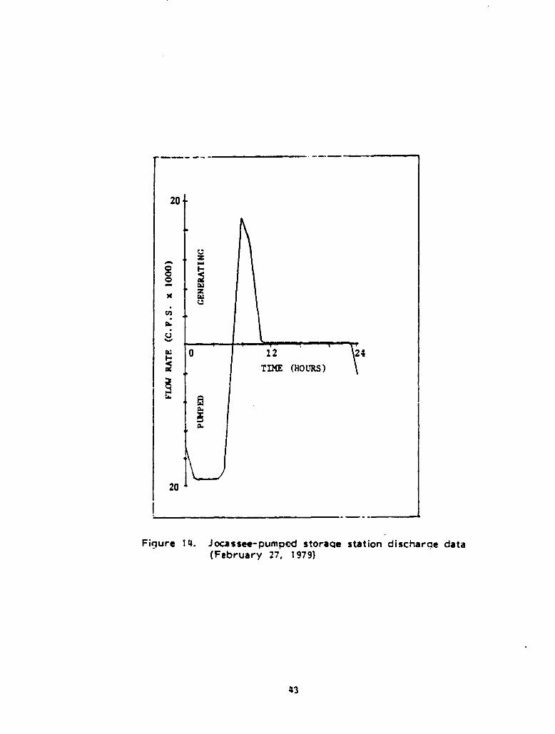
Figure 14. Jocassee-pumped stora ge station discharge data(February 27, 1979)
43

20 1
Figure 15. Jocassee-pumped stora ge station discharcte data(February 28, 1979)
44
16
000r•
x
G^
V gv3Oa
0 12 24TIME (HOURS)
Figure 16. Keowee hydro dischar ge (February 27, 1979)
45

0
x
vi 6
U
0 12 24
TIME (HOURS)
Figure 17. Keowee hydro discharge data (February 28, 1979)
46

VELOCITY SCALE(CM/SEC)0--n 0 30 .00L
RU N N3: LOt? I.
0 I CHSAIR0E "= • 3C I T ^.V 1 ^i L I r L V• V V L,,: v
01SCHARGE TEMPERA TUR 32 .3aCu1NO 0.0OniSECCURRENT 0.1 Ck-"SECTOTRL SI`ULRT=0 TIME 8 H=S
010`LENGTH SCRL = 0'00^(^I^TES) ^---
61 .00_1
• a qe_
Figure 18. Velocities at K = 1, Lake Keowee (rigid-lid model)
47
RUN ?42's L8 1,1 1 .011SIC i;R5E YEOCiTY i 5.4SCM,01SCH;FGE TEMPERATURE: 32.3^CWINu s 0.00rr/;CURAc' y T s 0.0 Ct1^ ^^^.T8TtiL S IMULRTEO TIME j 21 .SCHiiS
SCALES (H2_5I1?NT;L)
LENGTH SCALE(METERS)
VELaCITY SCALE(CM/SEC)
SCALES (VERTICAL)
LENGTH SCALE(M ETEFS)
VELBCITY SCALE(CM/SEA:)
x 10'0.00 51 .00
C . CC 12.CC
0.00 20.00
0 . 0 0 5.CC
Figure 19. Velocities at I = 11, Lake Keowee (rigid-lid model)
48
RUN N0: L00 1.DISCHARGE VELOCITY
DISCHARGE TEMPERATURE:
WINO
CURRENT
TOTRL SIMULATED TIME
LENGTH SCALE(METIERS)
VELOCITY SCRLE(CM/SEC)
5.65'M.'SEC32 .3aCO.00M/SEC0.0 C","SEc9 . 64 HRS
Vf 10`0.00 61 .00
0.0 0 30 •uCL J
ARCHTV A L DATA "IV - 5)
rREDiCTED - -•--•--
Figure 20. Isotherms: measured and predicted! (temperatures above ambient)
49

RUN NO % LOa 2.O ISCHRRJE YEL3C ITY 3 S .6SCI °EC
OISCHP.RGE TEMPERATURE, 32.310
WINO 0.00M/3EC
CURSENT 0.0 C't/ScCTOTAL SIMULRTED TIME 8.64 1RS
^' Qt
LENGTH SCRLE(METERS)0L00 611.00
VELOCITY SCALE(CM/SEC1(I 00 12.00
•I 1•
• . - • Ll • •
. . . . . . . . . .
Figure 21. Velocities at K = 1, Lake Keowee (ri g id-lid model)
50

RUN NO: L302.OISCHRRGE VELOCITY t S.SSC,.,/SECOISCHRRGE TEMAPERATURE s 32.3
13 C
WINO : 0 .00M/SECCURRENT 1 0 .0 Clti SECTOTAL SIMULATEO TIME : 8.S{ i:RS
SCALES (H:3R I T 'n NTnL IIt 0•
LENGTH SCALEcMETERS) C
t .00 61
^ .00
VELaCITY SCALE(CM/SEC) C . 00 12-00
Figure 22. Velocities at I = 11, Lake Keowee (rigid-lid model)
51

RUN tlfl 1 L 00 2. --
OISCHARGE VELOCITY 5.65CM/SEC IOISCHARGE TEMPERATURE% 32.390WINO 0 .001/ 3ECCURRENT 0.0 CrI/SECTOTAL SIMULATEO TIME 8.64 HRSviolLENGTH SCALE( M ETERS i
01.110 6I1 .00
VELOCITY SCALE(CM/SEC) 0 ,•00 12.00
aRCII IVAL D:^TA ("9,'10/75) .-9 :r---
PREDICTED — -• •—
Figure 23. Isotherms measured and predicted (temperatures above ambient)
52
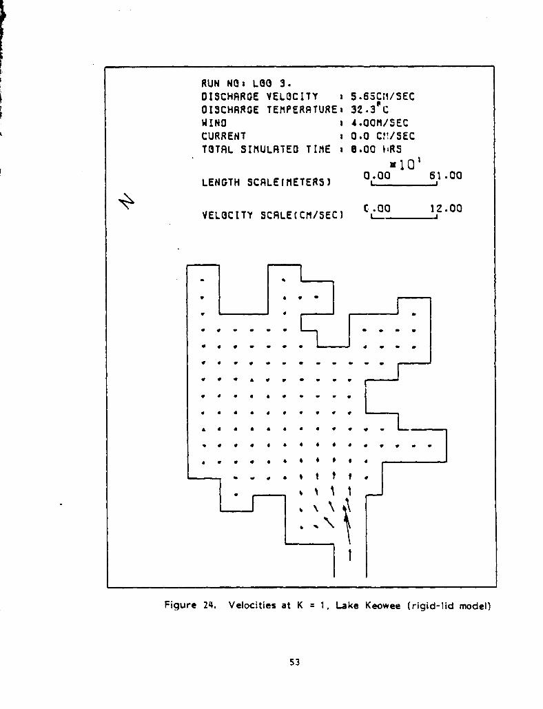
RUN N0: L00 3.OISCHARGE VELOCITY 5.65C(1/SEC
OISCHARGE TEMPERRTURE a 32.3 p
C
WINO 4•OOM/SEC
CURRENT i 0.0 Ct1/SECTOTAL SIMULATEO TIME 1 0.00 iiRS
a 10'LENGTH SCALE(METERS)
0 -- 61.00
VELOCITY SCALE(CM/SEC)G L0 0 12.00
. . . . . . . . . .
• . -
. . . . . . . . . .
. . . . . . . . . . .
t t t
4 1 1
Figure 24. Velocities at K = t , Lake Keowee (rigid-lid model)
53
^:.._.__ —_- - ._._ ___ _ - _ .. -
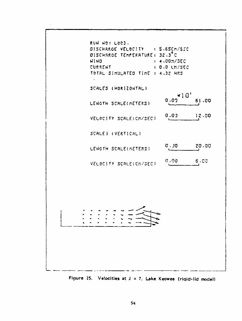
RUN 40 : L0C3 -01 SCHARCE VELOC! TY : 5.6SCM/S:COISCHSROE TEMPERATURE : 32.3@C
WINO
4.09M/SEC
CURZENT
0.0 LM/ SECTOTAL SIM ULATEO TI ME 4.32 HES
SCALES (HORIZONTAL)
LENGTH SCALE(nETERS)
VELOCITY SCALE(CM/SEC)
SCALES (VERTICAL)
LENGTH SCALE(METERS)
VELOC ITY SCALE(CM/SEC)
't 1 0'0 .01 61 .00
0.0^^ 12.00
o.jo zo.00
0 . QO 6 -Cct J
Figure 25. Velocities at J = 7, Lake Keowee (rigid-lid model)
54

VELOCITY SCALE(CM/SEC)0.00 12-00
RUN NO: Loa 3.OISCHARGE VELOCITY013CHARGE TEMPERATURE:WINO s
CURRENT s
TOTAL SIMULATEO TIME s
LENGTH SCALE(METERS)
5.65CM/SEC32 •34.ROM/SEC
0.0 VI/SEC8 .6t HRS
010'0.00 61 .00
1 f.C.111 'AL DATA ( 0!10/, ^ 1 x :r---
PREDICTED
Fig-ire 26. Isotherms: measured and predicted (temperatures above ambient)
55
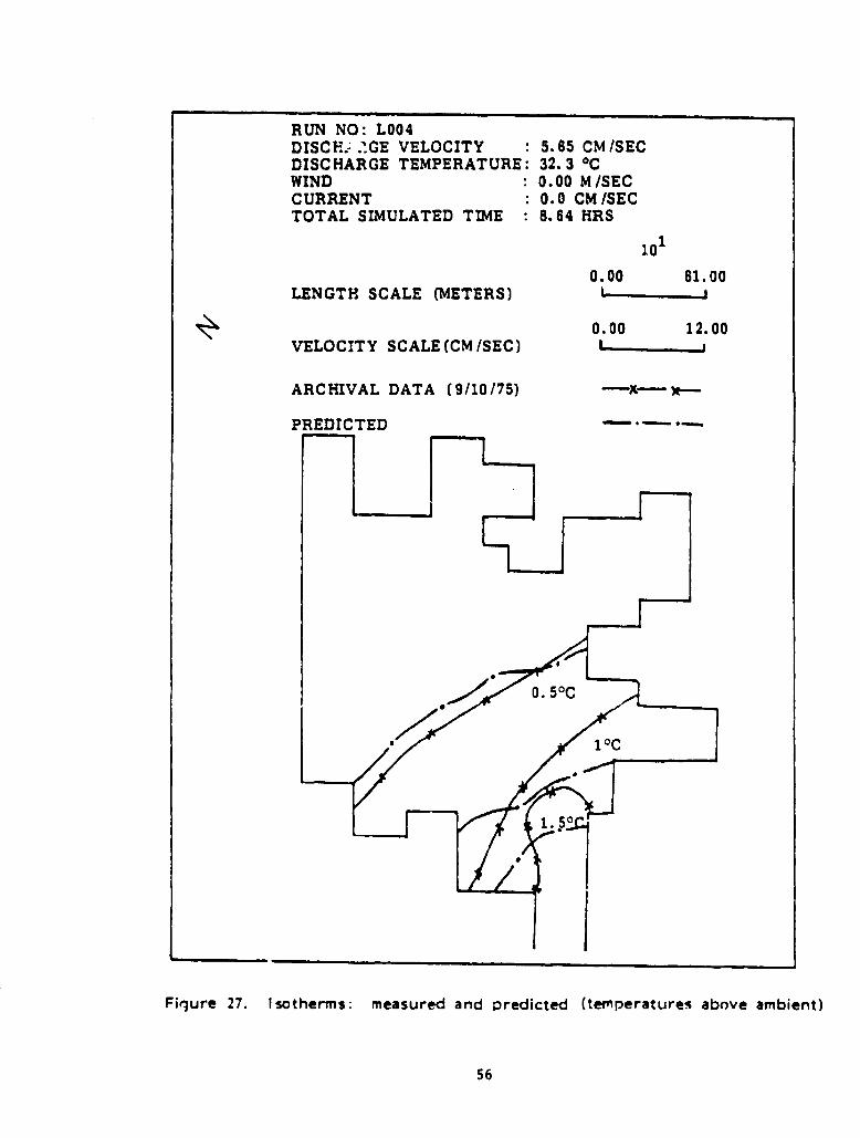
RUN NO: L004DISCFi:' ."GE VELOCITY 5.65 CM/SECDISCHARGE TEMPERATURE: 32.3 °CWIND 0.00 M /SECCURRENT 0.0 CM /SECTOTAL SIMULATED TIME 8.64 HRS
101
0.00 61.00LENGTH SCALE (METERS) ' j
0.00 12.00VELOCITY SCALE (CM /SEC) 1
ARCHIVAL DATA (9/10/75) x x
PREDICTED
Figure 27. Isotherms: measured and predicted (temperatures above ambient)
56
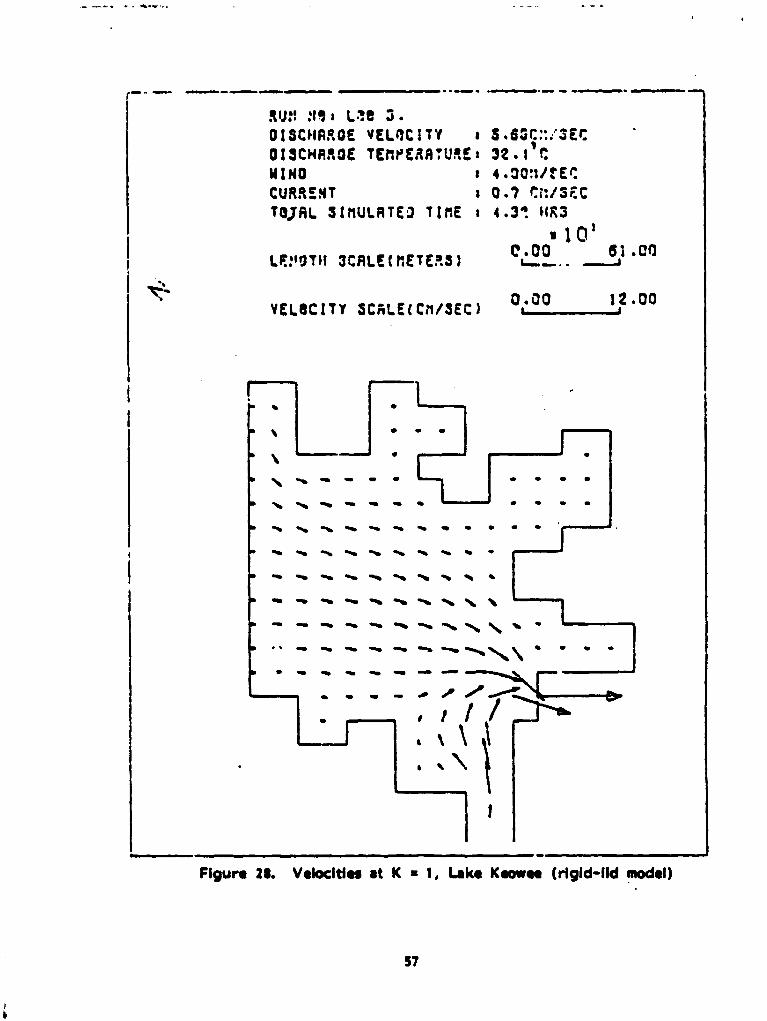
RU:! ;tI : t'6 a •DISCHARGE VEM I TY : S .Sat '.. M.01 3CHARCE TWERATURE: 32.1 1 r.NINO 4.00:1/4EcCURR;NT : 0.7 CIUS EC
TQJAI 3 I MULL TE J TI RE 1 4 . 31 HR3• 1 os
Lt;; 0 0T11 3CALE ( M ETER S) Ci__. .6j1 .QtI
YELeCITY SCAIECC A /SEC)01-00 1 2.00
d ^ Y
a •• + Li
I + ti ^ 1 1 ♦ 1♦ ♦ •
1
Figure 28. Velocities at K : 1, Lake Keowee (rigid-lid model)
r
57
UN V.i ' i 005 .CiSCNA4CEC iSCHA.ROE
N:NC:URREIN T
10)AL 3t'1
jCALE3 ! HOR:LON TAL )
LENGTH SCALE(METERS;
EL CC i T r SCPLE! Cili SEC
SCALES (VERTICAL)
ENCTM SCALE ( METERS)
ti ELOC t T ! SCALE (CI 3EC j
wiG'0 • Cie o ^ • 0^0
4 - UU '. 2 •00
u • Uu 20 . ^O
U • Uu G • U0
vELO^ I t r 5 .GS^'t, pctTEMPE,RP.TURE ^ S2 • 1^^
a .UO". ScC
ULATEC T iIE .:z • Ia'IR5
Figur* 29. Velocities at J a 7, Lake KeowN (rigid-Itd model)
58
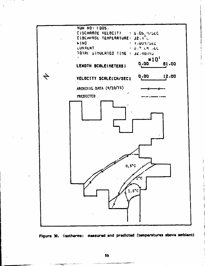
.RUN NQ, 1 00b.C I5CHARCE VELOCITY 5 -Gb, '1/:jLCCISCHHRGL TEMPERATURE . 32. 10+.
w 1 N 4 .UU1Ztir.lt.URAW u . 1 t.h ,EL101PI j IMULAIEG 1 1ME , ;e AUd,%4vio lLENGTH SCALEtMETERS)
a A 00^ 61.00
VELOCITY SCALE t CM/SEC 1 0_0^ 12.00
ARCHIVAL DATA (9/10/75)
PREDICTED f ...—
Figure 30. Isotherms: measured and predicted (temperatures above ambient)
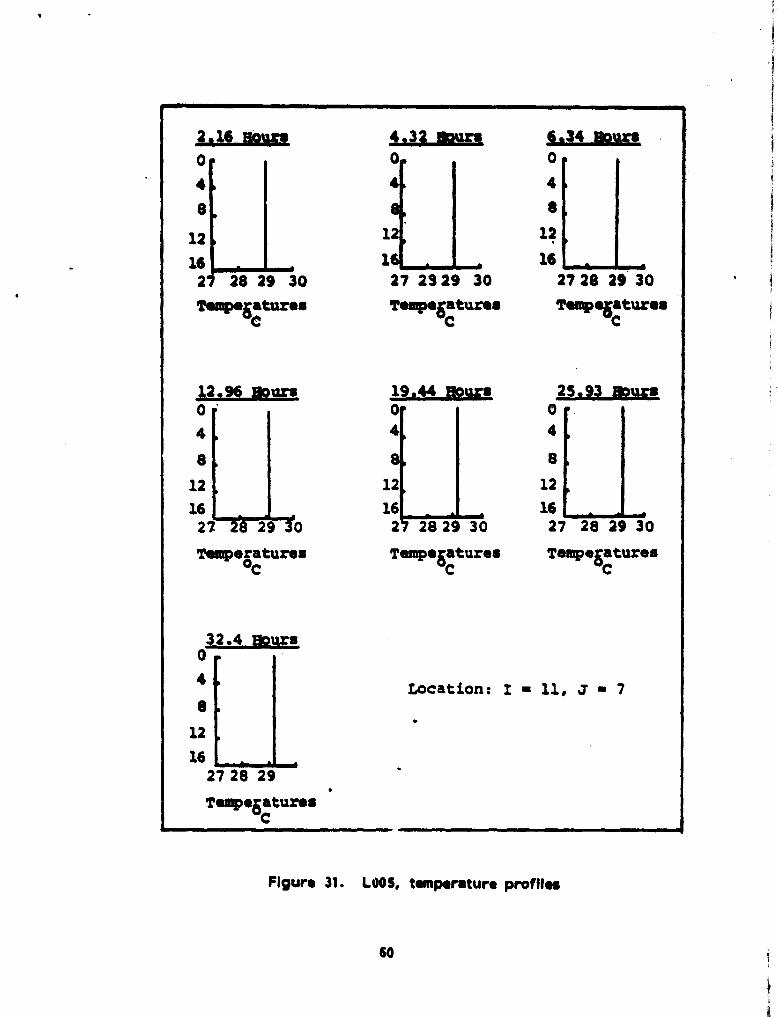
2.16
0
4
8
12
162f- 28 29 30
TanwsaturesC
4.32 Iffigan
27 2329 30
Tem"SaturesC
6.14 ggu—n0
4
8
12
16 Ld..L2728 29 30
ToVeg'aturesC
12.96 >gurs0'
4
8
12
1627 28 29 30
TeMorraturesC
1919="0
4
12
162 28 29 30
Ten"SaturesC
2
4
8
12
1627 28 29 30
TempegaturesC
3 2.4 Hours0
4
8
12
152728 29
TemperaturesC
Location: I = 11, J = 7
Figure 31. LOOS, temperature profiles
60

74-0 ^
u - velocity
3.0
umm
v2.0
"eV - veloci I
1.0
w - velocity
00 0
Time (lours)
Figure 32. L005, velocity vs. time, I = 11, J = 7, K = 1
61

9
V - velocity8
Ue7
vv>1 6
•r1
5
4
3
U - velocity2
w - velocity1
10 20 SOTime Sous
Figure 33. 100S, velocity vs. time, I = 11, J = 2, K = i
62

F
29.5
30.0
30.5
Ground Truth Correction 1.70C
Figure 38. IR data coreespondinq to 1002 hrs, Auqust 24, 1978, Lake Keowee
63

Figure 35. Isotherms at K = 1, Lake Keowee (rigid-lid model),simulations for Auqust 24, 1978
RUN N8+ L90 8-
OISCMAROE VELCICITY
013CHARGE TEMPERATURE#
WINO 3FEEO tMAX) i
CURRENT(JOCASEE FLOW)
TOTAL 31MULAYEO TIME I
LENGTH SCALE(METERS)
7.42CM/3EC32 .7eC3.Q2M/SEC1 -1 CM/SEC10.07HR3
• lot
0.00 61 .00
64
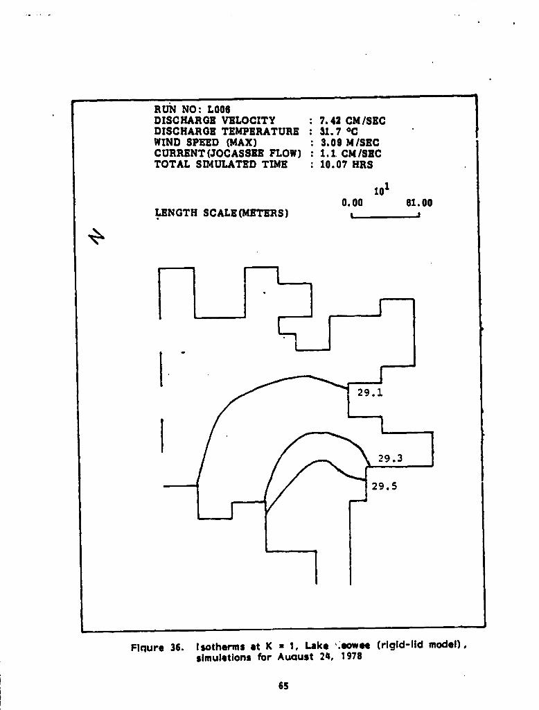
RUN NO: L008DISCHARGE VELOCITY : 7.42 CM/SECDISCHARGE TEMPERATURE : 91.7 °CWIND SPEED (MAX) : 3.09 N /SECCURRENT (JOCASSEE FLOW) : 1.1. CM /SECTOTAL SIMULATED TIME : 10.07 HRS
1010.00 61.00
LENGTH SCALE(METERS)
Fiqure 36. Isotherms at K = 1. Lake "eowee (rigid-lid model) ,simulations for Auqust 24, 1978
65

Temperature in 0C '
Ground Truth Correction +2.600
Fiqure 37. IR data corresponding to 0903-0953 hrs, Au gust 25, 1978 Lake Keowee
66
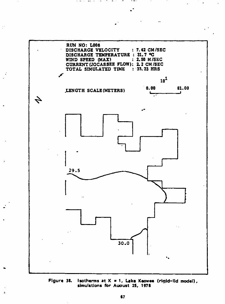
RUN NO: LOOS• DISCHARGE VELOCITY 7.42 CM /SEC
DISCHARGE TEMPERATURE 31.7 °CWIND SPEED (MAX) 2.50 M /SECCURRENT (JOCAS.SEE FLOW) : 2.2 CM /SECTOTAL SIMULATED TIME : '33. 23 HRS
101
,LENGTH SCALE(METERS) 0.00 61.00
Figure 38. Isotherms at K : 1, Lake Keowee (rigid-lid model),simulations for August 25, 1978
.
67

RUN NO: L008DISCHARGE VELOCITY 7.42 CM /SECDISCHARGE TEMPERATURE 31.7 °CWIND SPEED (MAX) 2.50 M /SECCURRENT (JOCAS.SEE FLOW) 1.1 CM /SECTOTAL SIMULATED TIME 33.2 HRS
101
LENGTH SCALE (METERS) 0.100 81.00
Figure 39. Isotherms at K a 1, Lake Keowee (rigld-lid model) ,simulations for Auqust 25, 1978
•
68
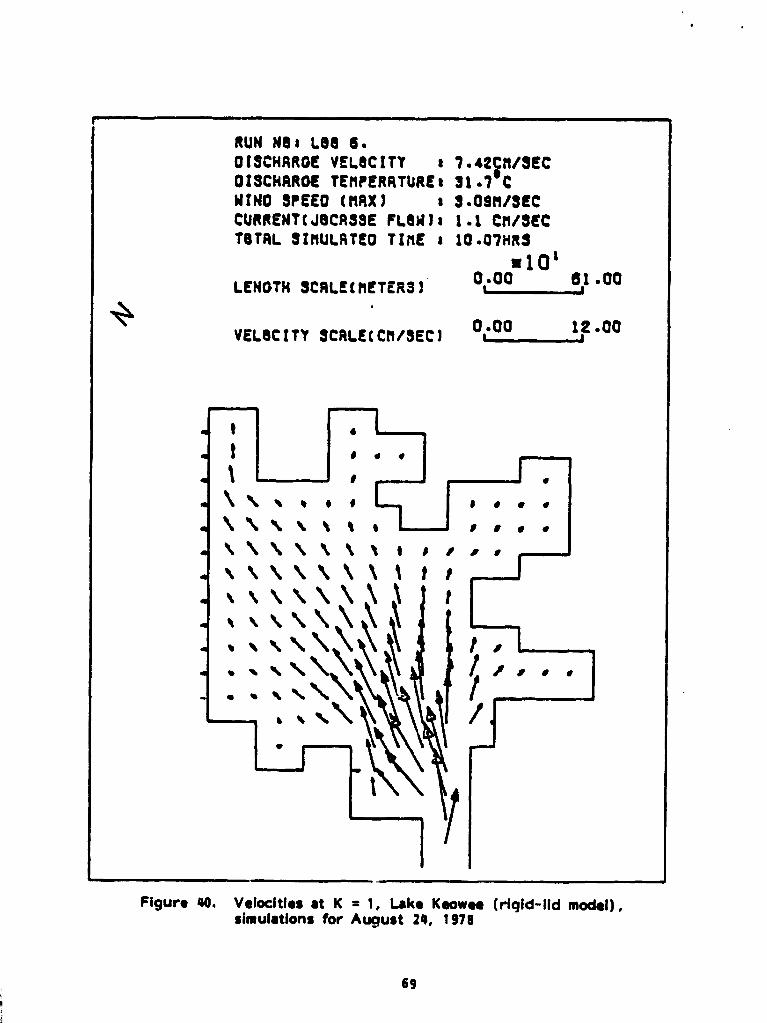
r
t
t
1
RUN NO$ LOO 0.DISCHARGE VELOCITY 7.t2f"/SECCtSCHRRGE TEMPERRTURII X1 .7 CWINO SPEED CMRX) 13-COM/3ECCURREWTCJOCA33E FLOW)$ 1.1 CM/3ECTOTRL SIMULRTEO TIME i 10.07MR3
=10'LENGTH 3CRLEtMETER3)
000 _ 61.00
VELOCITY SCRLEtCM/3EC)000 1 2.00
t L-,
^t
Fi t\\
Figure 40. Velocities at K = 1, Lake Keowee (rigid-lid model) ,simulations for August 24, 1978
69

RUN NO: LOO O•
DISCHARGE VELOCITY : 7.42CM/SEC013CHRROE TEMPERATURE= 31.7 1 C .WINO SPEED (MAX) : 3.09M/3ECCURRENT(JOCASSE FLOW)a 1.1 CM/SECTOTAL SIMULATED TIME i 34.24HR3
w1o,LENGTH SCALE(METERS)
0 00_ 61.00
VELOCITY SCALE(CM/SEC)000 12.00
t
•mot. ^ :
t ^, t ^^.NN
t
Figure 41. Velocities at K a 1, Lake Keowe♦ (rigid-lid model) ,simulations fnr August 25, 1978
70
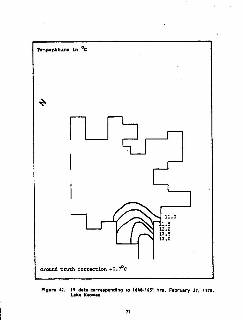
Temperature in °C
E-E
11.01.5
12.012.513.0
Ground Truth Correction +0.70C
Figure 42. IR data corresponding to 1648-1651 hrs, February 27, 1979,Lake Keowee
III
71

WWWW
RUN NO: L007DISCHARGEVELOCITY ' : 8.84 CM/SICDISCHARGE TRMPSRATURB : 18.4 °CNIHD SPEND MAY) : 2. 95 M /SICCURRENT (JOCA SNB FLOIr) ; 1.1 CM 18ECTOTAL SIMULATED TD4E 17.12 HRS
101
LENGTH SCALE (METERS) 0'` 61.00
0
Figure 43. Isotherms at K s 1, Lake Keowee (ricid-lid model),simulations for February 27, 1979
72
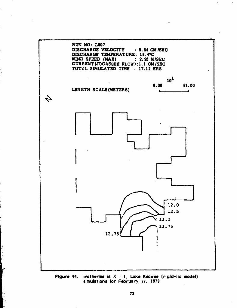
RUN NO: L007DISCHARGE VELOCITY 8.84 CM /SECDISCHARGE TEMPERATURE: 18.4°CWIND SPEED (MAX) : 2.95 M /SECCURRENT (JOCASSEE FLOW) :1.1 CM/SECTOTAL SIMULATED TIME : 17.12 HRS
101
0.00 81.00LENGTH SCALE (METERS) a
Figure 44. axotherms at K - 1. Lake Keowee (rigid-lid model)simulations for February 27, 1979
73
N\
;^ a

•
0
Temperaturt in 0C
Ground Truth Correction +1.30C
Figure 45. iR data corresponding to 0948-0957 hrs, February 28, 1979Lake Keowre
74
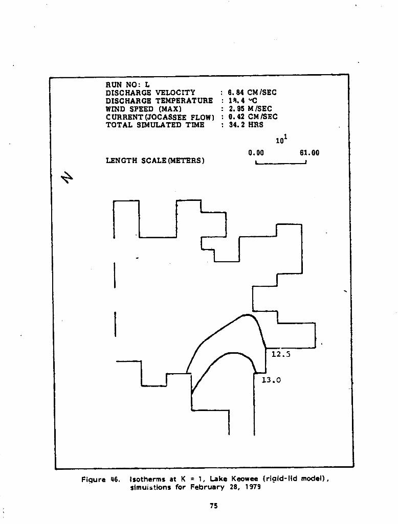
RUN NO: LDISCHARGE VELOCITY 6.84 CM/SECDISCHARGE TEMPERATURE 14.4 -CWIND SPEED (MAX) 2.95 M /SECCURRENT (JOCASSEE FLOW) 0.42 CM /SECTOTAL SIMULATED TIME 34.2 HRS
101
0.00 61.00LENGTH SCALE (METERS)
Fiqure 46, Isotherms at K = 1, Lake Keowee (ri g id-lid model) ,simuzitions for February 28, 1979
75
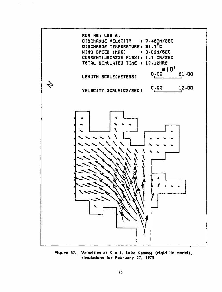
VELOCITY SCALE(CM/SEC)0.00 12.00
RUN NO s LOO 6 •
GISCHRRGE VELOCITY a 7.42CM/SECDISCHRRGE TEMPERRTURE s 31.7
4 C
WINO SPEED (MRX) s 3.09n/SEC
CURRENT(JOCRSSE FLOW), 1.1 Ch/SECTOTRL SI MU^RTED TIME s 17.12HRS
x1Q`LENGTH SCRLE(METERS)
0603 61.00
t t
i
Figure 47. Velocities at K = 1, Lake Keowee (ri g id-lid model),simulations for February 37, 1979
tt
1
76
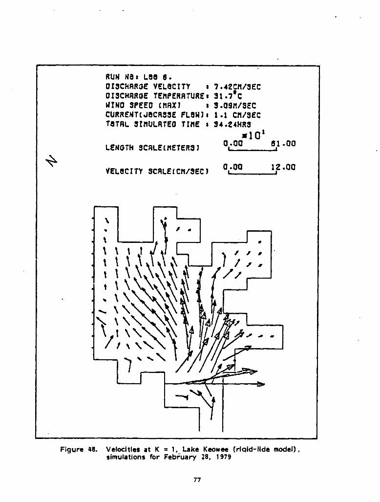
YELBCITY SCALE(CM/SEC)0.00 12.00
RUN Na s 1.88 6 •
OISCHAR3E YELBCITY s 7.42CH/3EC
DISCHARGE TEMPERATURE* 31.71CWINO SPEED (MAXI s 3.0911/SECCURRENT ( J8CA33E FL8W I s 1.1 CM /SECTBTAL 3iMULRTEG TIME s 34.24HRS
x10LENGTH SCALE(METER3 J 01-00 61-00
7^1
aw
Figure 48. Velocities at K = 1, Lake Keowee (rigid-fide model) ,simulations for February 28, 1979
77

Table 1. Monthly Gross Thermal Capacity Factors (Percent)for Oconee Nuclear Station .
MONTH 1973 1974 1975 1976 1977
Jan. 0 13 37 30 90
Feb. 0 28 22 49 77
Mar. 0 29 57 47 72
Apr. 0 26 61 27 92
May 4 5 76 33 76
Jun. 9 43 78 64 46
Jul. 15 38 80 59 44
Aug. 15 31 82 90 36
Sep. 16 46 76 77
Oct. 23 19 75 61
Nov. 23 31 92 52
Dec. 27 30 92 55
AnnualAverage 11 28 69 59
Data based on three-unit capability for entire period.
Gross Thermal Actual MWH (t) x 100Capacity Factor = 770 4 MW (t) x Hours in Perinfor ONS M
78

Table 2. Operating Conditions of Oconee Nuclear Power Plantat Lake Keowee (September 10. 1975)
Flow Rate : 7087 m /min
Inlet Temperature . 26.6 °C
Outlet Temperature . 32.4 °C
The hourly averages of wind. air temperature andrelative humidity:
Time WindS eed (MPH)
WindDirection (°N)
AirTemp.
RelativeHumidity
9: 00 7.7 15 69.0 100
10:00 6.8 65 74.0 70
11:00 8.3 80 77.0 60
12:00 7.2 95 77.0 63
13:00 9.7 115 78.0 66
14:00 11.3 205 79.0 84
15:00 - - 77.0 66
16:00 10.2 75 73.0 84
79
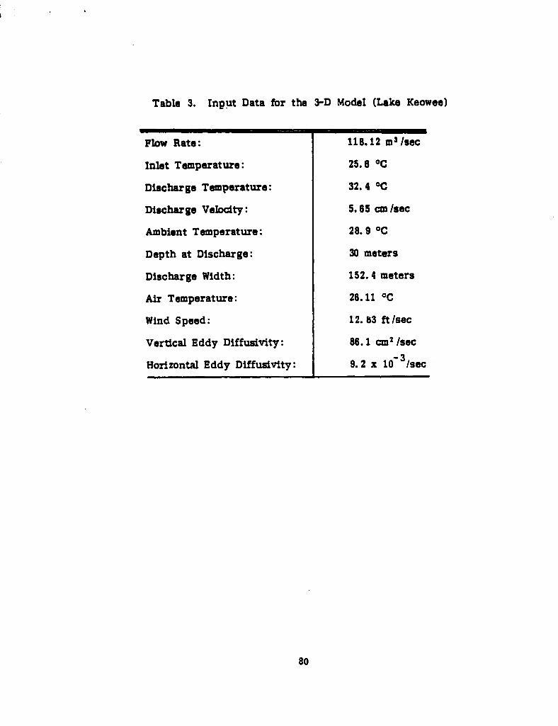
Table 3. Input Data for the 3-D Model (Lake Keowee)
Flow Rate: 118.12 m a /sec
Inlet Temperature: 25.6 °C
Discharge Temperature: 32.4 °C
Discharge Velocity: 5.65 cm /sec
Ambient Temperature: 28.9 °C
Depth at Discharge: 30 meters
Discharge Width: 152.4 meters
Air Temperature: 26.11 °C
Wind Speed: 12. 83 ft /sec
Vertical Eddy Diffusivity: 86.1 =2 /sec
Horizontal Eddy Diffusivity: 9.2 x 10 3 /sec
80

Table 4. Volume and Area Data for Lake Keowee
*M
WATER SURFACEELEVATION(m) (ft.)
SURFACE AREA(SQ. KM .)
STORAGE VOLUME
(109 m
246.9 810 83.3 1.42
245.4 805 78.8 1.30
' 243.8 800 74.4 1.18
242.3 795 70.1 1.07
240.8 790 65.8 0. 13
239.3 785 61.2 0.87
237.7 780 56.6 0.78
237.1 778 55.1 0.75
' 236.2 775 52.8 0.70
234.7 770 48.9 0.62
231.6 760 41.5 0.48
228.6 750 35.3 0.36
225.6 740 27.8 0.27
222.5 730 22.5 0.19
219.4 720 17.8 0.13
216.4 710 13.2 0.08
213.4 700 9.6 0.05
210.3 690 5.7 0.02
207.3 680 3.1 0.01
204.2 670 1.3 0.004
201.2 680 0.6 0.001
198.1 650 1 0.3 -----
* Full Pond
** Maximum Allowable Drawdow-r
8?

Table 5. Inflows and Outflows to Laker Y.eowee, August 24. 1978
TIME
Aug. 241978
OCONEEDISCHARGE
(m3 /min)
OCONEEDISCHARGE
TEMP.
°C
NET JOCASSEEFLOW
(CFS)
KEOWEEHYDRO FLOW
(CFS)
12.00 AM 8172.9 31.8 -2638 663601.00 8177.5 31.8 -6059 669602.00 8178.6 31.9 -7982 541603.00 8180.1 32.1 -12036 541604.00 8185.4 32.3 -12066 675805.00 8179.4 32.4 -11985 227606.00 8181.7 32.5 -10598 4807.00 8313. ^ 32.3 -5970 4808.00 8183.5 32.4 -995 4809.00 8176.4 32.5 100 4810.00 8183.9 32.5 100 4811.00 8177.1 32.5 100 4812.00 PM 8159.9 32.6 100 481.00 8155. 9 32.6 100 482.00 8247.2 32.7 100 483.00 8169.5 32.7 100 484.00 8438.7 32.4 100 485.00 7935.2 30.7 8726 142246.00 75' 31.0 10905 84327.00 8091.:, 30.3 9823 454.48.00 8119.6 30.2 4557 -189.00 8132.8 30.2 6482 4810.00 8141.9 30.2 4183 4811.00 8143.8 30.2 100 4812.00 AM 8151.8 30.3 100 48
82

Table 6. Inflows and Outflows to Lake Keowee, August 25, 1978
TIME
Aug. 251978
OCONEEDISCHARGE
(m3 /min)
OCONEEDISCHARGE
TEMP.
°C
NET JOvASSEEFLOW
(CFS)
KEOWEEHYDRO FLOW
(CFS)
12.00 AM 8151.8 30.3 100 48
1.00 7952.3 28.9 4938 3576
2.00 7097.2 2& 5 838 608
3.00 7398.4 29.1 100 48
4.00 7098.8 29.6 101t) 48
5.00 7103.7 30.0 100 48
6.00 7102.6 30.5 100 48
7.00 7104.4 30.7 100 48
8.00 7279.7 30.9 100 3484
9.00 8012.8 30.5 100 8624
10.00 7760.4 30.7 100 9352
11.00 7759.2 30.9 100 1392
12.00 PM 8059.8 30.7 1632 2564
1.00 8130.6 30.8 5442 8820
2.00 8112.8 30.9 11553 9500
3.OG 8141.9 31.1 19048 7624
4.00 8102.2 31.3 17180 7856
5.00 8108.6 31.3 10615 8852
6.00 8107.5 31.4 10158 8172
7.00 8110.1 31.5 10076 2660
8.00 8114.7 31.5 2185 48
9.00 8126.8 31.5 29.83 48
10.00 8148.3 31.5 3151 48
11.00 8141.9 30.4 2647 48
12.00 AM 8141. 9 30.3 100 48
83
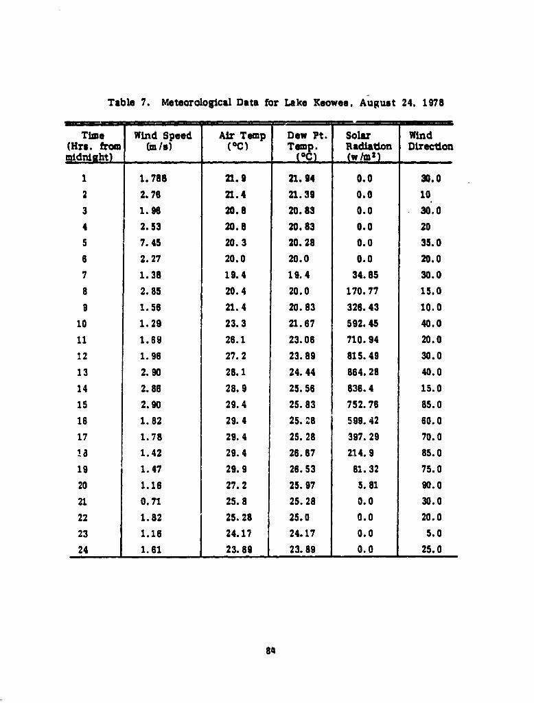
Table 7. Meteorological Data for Lake Keowee, August 24, 1978
TimeMrs. frommidni bt
Wind Speed(in /a)
Air Temp(°C)
Dew Pt.Temp.
°C
SolarRadiation
w /m =
WindDirection
1 1.788 21.9 21.94 0.0 30.0
2 2.76 21.4 21.39 0.0 10
3 1.96 20.8 20.83 0.0 30.0
4 2.53 20.8 20.83 0.0 20
5 7.45 20.3 20.28 0.0 35.0
6 2.27 20.0 20.0 0.0 20.0
7 1.38 19.4 19.4 34.85 30.0
8 2.85 20.4 20.0 170.77 15.0
9 1.56 21.4 20.83 326.43 10.0
10 1.29 23.3 21.67 592.45 40.0
it 1.69 26.1 23.06 710.94 20.0
12 1.96 27.2 23.89 815.49 30.0
13 2.90 28.1 24.44 864.28 40.0
14 2.86 28.9 25.56 836.4 15.0
15 2.90 29.4 25.83 752.76 85.0
16 1.82 29.4 25.28 599.42 60.0
17 1.78 29.4 25.28 397.29 70.0
d 1.42 29.4 26.67 214.9 85.0
19 1.47 29.9 26.53 81.32 75.0
20 1.16 27.2 25.97 5.81 90.0
21 0.71 25.8 25.28 0.0 30.0
22 1.82 25.28 25.0 0.0 20.0
23 1.16 24.17 24.17 0.0 5.0
24 1.61 23.89 23.89 0.0 25.0
84

Table S. Meteorological Data for Lake Keowee
Time(Hre . ft=midni ht
Wind Speed(m /4)
Air Temp(°C)
Dew Pt.Tamp.
°C
SolarRadiation
w /m
WindDirection
a ees
1 1.028 23.1 23.0 0.0 55.0
2 2.951 23.1 23.0 0.0 40.0
3 2.414 22.2 22.2 0.0 20.0
4 2.995 22.2 22.2 0.0 55.0
5 1.833 21.9 21.9 0.0 30.0
6 1.833 21.7 21.7 0.0 35.0
7 2.235 21.4 21.4 0.0 25.0
8 1.922 21.7 21.7 27.89 40.0
9 1.833 23.3 20.0 168.52 10.0
10 0.760 25.3 17.2 348.67 15.0
11 1.162 26.9 18.3 534.62 10.0
12 1.565 28.6 16.1 891.52 45.0
13 1.654 29.7 16.9 796.12 55.0
14 1.967 30.6 16.7 1041.35 55.0
15 2.503 30.8 16.1 807.74 70.0
18 2.012 30.8 18.1 708.96 45.0
17 2.056 30.8 16.7 575.30 55.0
18 1.743 30.0 20.0 284.74 90.0
19 1.967 29.4 22.7 185.96 80.0
20 1.854 28.3 21.1 58.11 ".0
21 2.414 27.2 25. " 0.0 65.0
22 1.341 25.8 25.6 0.0 90.0
23 1.073 25.6 2.3.6 0.0 10.0
24 3.085 25.6 25.6 0.0 40.0
85
3
-im-

i
0
Table 9. Inflows and Outflows to Lake Keowee. February 27, 1979
TIME
Feb. 27,1978
OCONEEDISCHARGE
(m3 /Min)
OCONEEDISCHARGE
TEMP.(°C)
NET JOCASSEEFLOW
(C.F.S.)
KEOWEE HYDRFLOW
(C.F.S.)
12.00 AM 7505.3 18.6 -14395 48
1.00 7498.1 18.5 -18754 48
2.00 7492.0 18.4 -18805 48
3.00 7492.0 18.5 -18713 484.00 7491.6 18.3 -18698 48
5.00 7494.3 18.3 -18688 48
8.00 7488.2 18.3 -15939 487.00 7481.8 18.2 3484 36688.00 7485.6 18.3 16823 175409.00 7488.2 18.2 13503 848810.00 7497.7 18.3 5470 +109611.00 7504.1 18.3 100 268012.00 PM 7503.4 18.4 100 481.00 7506.0 18.5 100 482.00 7506.4 18.5 100 48
3.00 7503.4 18.5 100 48
4.00 7501.9 18.4 100 485.00 7507.5 18.4 100 48
6.00 7511.0 18.4 100 48
7.00 7516.2 18.4 100 48
8.00 7518.9 18.3 100 1 A
9.00 7520.4 18.3 100 4810.00 7516.6 18.2 100 48
11.00 7509.4 18.2 100 48
12.00 AM 7507.2 18.2 -4382 48
86

Table 10. Inflows and Outflows to Lake Keowee, February 28. 1979
TIME
Feb. 28,1978
OCONEEDISCHARGE
(m'/min)
OCONEEDISCHARGE
TEMP.
(°C)
NET JOCASSEEFLOW
(C.F.S.)
KEOWEE HYDROFLOW
(C.F.S.)
12.00 AM 7507.2 18.2 -4382 48
1.00 7616.4 19.8 -18050 48
2.00 7655.5 19.5 -18621 48
3.00 7356.3 19.8 -18602 48
4.00 7233.4 20.1 -18692 48
5.60 7494.7 19.5 -18559 48
6.00 7605.3 19.1 -15139 48
7.00 7618.6 19.1 3045 48
8.00 7300.2 19.5 19245 5788
9.00 7239.8 19.5 8338 48
10.00 7241.9 19.4 100 48
11.00 7243.0 19.3 100 48
12.00 PM 7246.2 19.1 100 48
1.00 7239.0 19.0 100 48
2.00 7241.0 18.9 100 48
3.00 7235.3 18.9 100 48
4.00 7207.8 18.9 100 48
5.00 7196.3 18.7 100 48
6.00 7200.0 18.9 100 48
7.00 7211.5 19.2 100 48
8.00 7212. 19.0 100 48
9.00 6829.4 18.3 100 48
10.00 7189.1 '18.5 100 48
11.00 7287.8 18.1 -1544 48
12.00 AM 7036.7 15.8 -15141 48
_b 87
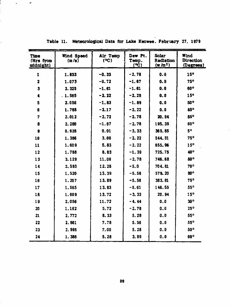
Table 11. Meteorological Data for Lake Keowee. February 27. 1979
TimeMrs frommidnight)
bind Speed(m /s)
Air Tamp(°C)
Dew Pt.Temp.
°C)
SolarRadiation
w /m 2 )
WindDirection
e s
1 1.833 -0.33 -2.78 0.0 1510
2 1.073 -0.72 -1.67 0.0 750
3 2.325 -1.61 -1.61 0.0 600
4 .1.565 -2.22 -2.28 0.0 150
5 2.056 -1.83 -1.89 0.0 50°
6 1.788 -2.17 -2.22 0.0 850
7 2.012 -2.72 -2.78 20.94 85°
8 2.280 -1.67 -2.78 195.39 600
9 0.626 0.01 -3.33 369.85 50
10 1.386 3.06 -2.22 544.31 750
11 1.609 5.83 -2.22 655.96 150
12 1.788 8.83 -1.39 725.75 400
13 3.129 11.06 -2.78 746.68 800
14 2.593 12.28 -5.0 704.81 700
15 1.520 13.39 -5.56 579.20 800
16 1.207 13.89 -5.56 383.81 750
17 1.565 13.83 -5.61 146.55 550
18 1.609 13.72 -3.33 20.94 150
19 2.056 11.72 -4.44 0.0 300
20 1.162 9.72 -2.78 0.0 250
21 2.772 8.33 5.28 0.0 550
22 2.861 7.018 5.58 0.0 550
23 2.995 7.00 5.28 0.0 50°
24 1.388 5.28 3.89 0.0 60°
88

Table 12. Meteorological Data for Lake Reowee, February 28. 1979
TimeMrs. frommid night)-
Blind Speed(m/8)
Air Tamp(°C)
Dew Pt.Temp.
°C
SolarRadiation
w /m z )
BlindDirection(Degrees)
1 2.280 4.94 4.17 0.0 55
2 2.101 4.00 4.17 0.0 55
3 1.967 3.00 2.22 0.0 60
4 2.414 2.28 1.67 0.0 505 2.593 f 2.61 2.22 0.0 80
6 4.068 4.11 3.06 0.0 75
7 3.398 3.83 0.28 20.94 60
8 3.934 4.22 -2.78 153.52 60
9 4.515 6.67 -3.89 279.13 85
10 4.381 7.78 -5.00 439.64 60
11 3.710 9.28 -5.00 676.90 70
12 2.235 10.78 -3.89 907.18 45
13 1.878 11.72 -3.89 537.33 60
14 1.609 12.28 -3.89 565.24 50
15 3.442 13.33 -3.33 6 90.85 45
16 2.950 13.61 -2.78 0.0 4517 2.325 13.33 -1.67 0.0 45
18 2.012 12.72 -0.56 0.0 5
19 2.235 11.39 1.39 0.0 65
20 2.950 10.39 2.28 0.0 55
21 2.772 10.61 2.22 0.0 85
22 2.638 10.44 2.22 0.0 50
23 2.191 10.00 2.22 0.0 65
24 2.369 9.83 2.22 0.0 70
89
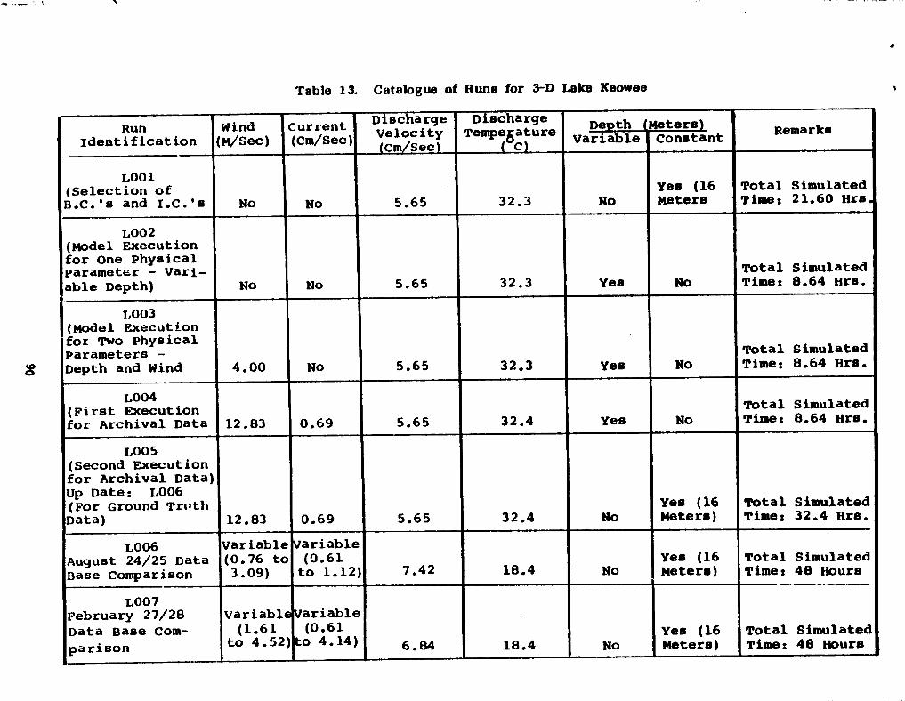
t
meoIDacaoWmwOWO
.^U.•+
1
,aj
cc
F
m M
^C 110^ tl 1
d M
^ tl I^ a D
41 O!41 L
ii^ T
•i^
1.141 N
iJ la
41 $1
41 L
I??
mr-4
54ro.r1o-4
-P4I•
.14•
•rl•
Yi N
"4C
D'•^
^^
to Nt11 to
to mN
mG
/1 e +1d1 d
'O
d'
IV
IM/
N♦to
ICIN
,^ m
/^I
••
ro ro
^ ••
ror4••
gom
P4•'
ro c^P4N
^o
E E
E-46 E
+E
EE
-4 E-4
E E
E-4 E-4
CtC
^ .^
^ y
^" yl^ f.i
v fl
v t,i
ZZ
Zm
^+
q ^
. ►m
++
4+
Om
mVp
w+
'+
ca $+ro
m^I.IO
,CN
NN
NN
mm
U a
l—e•1
e1tr1
e+1e•1
.••I.-1
m00E
m ^41 u
to t!1
%D
m ^
U
O
Os4
Nmro
^ •
,,4
;^
xz
zo
a 0
0$
40
c o
v --4) ^
NA
f-4 U
*t
^o
evim
(ncoA^^a
►ro
`0
'
ca^
xi nO
^''i^
C^
;per
;`m
ay
...
roC
m
Aro
p"4u
0 1
>a
.04 U to
oro
-,4 U
^aoro
•.+ a
•Aro
:141 a %
o $+o
o,
m^U
N U
>• I .-.
t•1 U
> 43
d' U
rotl1 y
ro ra ' C
t0 N L
it` r-
C ••+O
CIO
O G
I .0 ,C
O O
t toO
m>
O i4 >
CO
\ rtfO
N
0^
a°+
co°a^
au"Ia
ar^°'a", c°a
^c
aw
e ••c
aN
^'a>,°%
ro c
A,
41a y
al
o +
+ ro
U10 U
0 1
+o
$4m
0C
U aD
o-4
C G
I A•"I 3
CIAi w
C 1r 41 t7+J U
rom
4)-
OO
Em
EE
Aa0
40
4ro
.-.m
a
H^U
f-4 a
•^1a^^O
O^
a+^A
+J•N
^wa^
=-wao
^w^w
a^Aam
io.o
r.^06
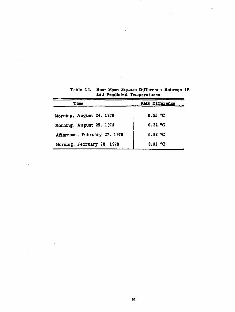
Table 14. Root Mean Square Difference Between IRand Predicted Temperatures
D
Morning, August 24, 1978 0. 55 °C
Morning, August 25, 1973 0. 34 °C
Afternoon, February 27, 1979 0.82 °C
Morning, February 28, 1979 0.01 °C
91