Model theory for extensions of modal logic -...

Model theory for extensions ofmodal logic

Balder ten Cate and David Gabelaia

ESSLLI 200820th European Summer School in Logic, Language and Information4–15 August 2008Freie und Hansestadt Hamburg, Germany

Programme Committee. Enrico Franconi (Bolzano, Italy), Petra Hendriks (Groningen, TheNetherlands), Michael Kaminski (Haifa, Israel), Benedikt Lowe (Amsterdam, The Netherlands& Hamburg, Germany) Massimo Poesio (Colchester, United Kingdom), Philippe Schlenker (LosAngeles CA, United States of America), Khalil Sima’an (Amsterdam, The Netherlands), RinekeVerbrugge (Chair, Groningen, The Netherlands).

Organizing Committee. Stefan Bold (Bonn, Germany), Hannah Konig (Hamburg, Germany),Benedikt Lowe (chair, Amsterdam, The Netherlands & Hamburg, Germany), Sanchit Saraf (Kan-pur, India), Sara Uckelman (Amsterdam, The Netherlands), Hans van Ditmarsch (chair, Otago,New Zealand & Toulouse, France), Peter van Ormondt (Amsterdam, The Netherlands).

http://www.illc.uva.nl/ESSLLI2008/

[email protected]

ESSLLI 2008 is organized by the Universitat Hamburg under the auspices of the Association for Logic, Language andInformation (FoLLI). The Institute for Logic, Language and Computation (ILLC) of the Universiteit van Amsterdam isproviding important infrastructural support. Within the Universitat Hamburg, ESSLLI 2008 is sponsored by the Depart-ments Informatik, Mathematik, Philosophie, and Sprache, Literatur, Medien I, the Fakultat fur Mathematik, Informatikund Naturwissenschaften, the Zentrum fur Sprachwissenschaft, and the Regionales Rechenzentrum. ESSLLI 2008 isan event of the Jahr der Mathematik 2008. Further sponsors include the Deutsche Forschungsgemeinschaft (DFG), theMarie Curie Research Training Site GLoRiClass, the European Chapter of the Association for Computational Linguistics,the Hamburgische Wissenschaftliche Stiftung, the Kurt Godel Society, Sun Microsystems, the Association for SymbolicLogic (ASL), and the European Association for Theoretical Computer Science (EATCS). The official airline of ESSLLI 2008is Lufthansa; the book prize of the student session is sponsored by Springer Verlag.


Model theory for extensions ofmodal logic

Course Material. 20th European Summer School in Logic, Lan-

guage and Information (ESSLLI 2008), Freie und Hansestadt Ham-

burg, Germany, 4–15 August 2008

The ESSLLI course material has been compiled by Balder ten Cate and David Gabelaia. Unless otherwise mentioned,the copyright lies with the individual authors of the material. Balder ten Cate and David Gabelaia declare that theyhave obtained all necessary permissions for the distribution of this material. ESSLLI 2008 and its organizers take no legalresponsibility for the contents of this booklet.

iii

Model theory for extensions of modal logic


ESSLLI 2008

Table of content

Part 1. Modal model theory . . . . . . . . . . . . . . . . . . . . . . . . . . . . . . . . . . . . . . . . . . . . . . . . 1

Part 2. Topological semantics for modal logic . . . . . . . . . . . . . . . . . . . . . . . . . . . . . .35

Part 3. Expressivity and definability for extended modal languages . . . . . . . . 69

About this reader

The main purpose of this reader is to provide a convenient source of referencefor some of the things that will be discussed in the course. We do not intend tocover all of this material in the course.

This reader has been compiled out of material from the following three sources:

• Balder ten Cate (2005). Model theory for extended modal languages.PhD thesis, University of Amsterdam. Available from http://staff.

science.uva.nl/∼bcate

• David Gabelaia (2001). Modal definability in topology. Master’s thesis,University of Amsterdam. Available from http://www.science.uva.nl/

pub/theory/illc/researchreports/MoL-2001-11.text.pdf

• Balder ten Cate, David Gabelaia, and Dmitry Sustretov (2006). Modallanguages for topology: expressivity and definability. Available fromhttp://arxiv.org/abs/math/0610357

Part I

Modal model theory

Chapter 1

Background

1.1 Basics of model theory

This section reviews a number of important results on the model theory of firstorder logic that are used in proofs throughout these course notes. For a more de-tailed treatment, cf. [17, 9]. We assume that the reader is familiar with the syntaxand semantics of first-order logic. We will only consider first-order languages withconstants and relation symbols and without function symbols of arity greater thanzero. We will denote first-order models (or, structures) as pairs M = (D, I) con-sisting of a domain D and an interpretation function I that assigns relations ofthe appropriate arity to the relation symbols and that assigns elements of D toconstants. Given such a structure M and a first-order formula ϕ(x1, . . . , xn), wewill write M |= ϕ [d1, . . . , dn] if d1, . . . , dn are elements of the domain of M, suchthat ϕ holds in M interpreting x1, . . . , xn as d1, . . . , dn.

The first three results are easily stated.

1.1.1. Theorem (Compactness). Let Σ be a set of first-order formulas. Ifevery finite subset of Σ has a model, then Σ has a model.

1.1.2. Theorem (Lowenheim-Skolem). Let Σ be a countable set of first-order formulas. If Σ has a model then Σ has a countable model.

1.1.3. Theorem (Craig Interpolation). Let ϕ, ψ be first-order formulas,such that |= ϕ→ ψ. Then there is a formula ϑ such that |= ϕ→ ϑ, |= ϑ→ ψ andall constants, relation symbols and function symbols occurring in ϑ occur both inϕ and in ψ.

For the remaining results we need to introduce some terminology. A model M

is a submodel of a model N if the domain of M is a subset of the domain of N

and the interpretations of every non-logical symbol in M is simply the restrictionof its interpretation in N with respect to the domain of M. It follows that if anelement of the domain of N is named by a constant, then it is also in the domain

3

4 Chapter 1. Background

of M. We say that M is an elementary submodel of N if it is a submodel, andfor all first-order formulas ϕ(x1, . . . , xn) and elements d1, . . . , dn of the domain ofM, M |= ϕ [d1, . . . , dn] iff N |= ϕ [d1, . . . , dn]. In this case, we also say that N isan elementary extension if M.

Given a set of models {Mi | i ∈ I} for a relational language (i.e., without con-stants or function symbols), the union N =

⋃

i∈I Mi is defined in the natural way:the domain of N is the union of the domains of Mi (i ∈ I), and the same holdsfor the interpretation of the relation symbols. In general, this notion can onlybe applied to models for relational languages. However, there are circumstancesin which it can also be applied to models for languages containing constants andfunction symbols. An example of this is the following situation.

1.1.4. Theorem (Unions of elementary chains). Let (Mk)k∈ω be a se-quence of models, such that Mk is an elementary submodel of Mk+1 for all k ∈ ω,and let Mω be the union

⋃

k∈ω Mk. Then for each k ∈ ω, Mk is an elementarysubmodel of Mω.

NB:⋃

i∈I Mi should not be confused with the disjoint union of the models Mi

(i ∈ I). In fact, for the above result crucially relies on the non-disjointness of themodels in question.

An ultrafilter over a set W is a set U ⊆ ℘(W ) satisfying three conditions:

1. W ∈ U

2. For all X ⊆ W , X ∈ U iff (W \X) 6∈ U

3. For all X ∈ U and Y ∈ U , X ∩ Y ∈ U

An ultrafilter is principal if has a singleton element.

1.1.5. Definition (Ultraproducts). Given a collection of models {Ma =(Da, Ia) | a ∈ A} and an ultrafilter U over the set A, the following defines theultraproduct ΠUMa = (D, I).

Let ∼ be the equivalence relation ∼ on the product Πa∈ADa given by

f ∼ g iff {a ∈ A | f(a) = g(a)} ∈ U

Let D be the quotient (Πa∈ADa)/ ∼. For each constant c, let

I(c) = [〈Ia(c)〉a∈A]∼

Finally, for each k-ary relation R and [f1], . . . , [fk] ∈ D, let

([f1], . . . , [fk]) ∈ I(R) iff {a ∈ A | (f1(a), . . . , fk(a)) ∈ Ia(R)} ∈ U

1.1. Basics of model theory 5

If all factor models Ma are the same, then ΠUMi is called an ultrapower. Everymodel M is isomorphic to a submodel of the ultrapower ΠUM, the isomorphismbeing the function that sends every element d to the equivalence class [〈d, d, . . .〉]∼.

1.1.6. Theorem ( Los). For all models M, ultrafilters U and first-order sen-tences ϕ, ΠUM |= ϕ iff M |= ϕ

Related to ultraproducts are the simpler notions of products and subdirect prod-ucts, which will also play a role in this thesis.

1.1.7. Definition (Products and subdirect products). The product ofa collection of models {Ma = (Da, Ia) | a ∈ A}, (also called cartesian prod-uct or direct product, notation: Πa∈AMa) is the model (D, I), where D is thecartesian product Πa∈ADa, and for each n-ary relation R,

I(R) = {〈d1, . . . , dn〉 ∈ Dn | 〈d1(a), . . . , dn(a)〉 ∈ Ia(R) for each a ∈ A}

A subdirect product of {Ma | a ∈ A} is any submodel N of the product Πa∈AMa

for which it holds that the natural projection functions from the domain of N tothe domains of the models Ma (a ∈ A) are surjective.

The next notion we introduce is that of ω-saturatedness. A 1-type is a set offormulas in one free variable. A 1-type Γ(x) is realized in a model M if there isan element d of the domain of M such that M |= Γ [x : d]. A model is said tobe 1-saturated if for all 1-types Γ(x), if every finite subset of Γ(x) is realized inM, then Γ(x) itself is realized in M. One can think of 1-saturatedness as a sortof compactness within a model.

Given a model M and a finite sequence d1, . . . , dn of elements of the domainof M, we use (M, d1, . . . , dn) to denote the expansion of M in which the ele-ments d1, . . . dn are named by additional constants c1, . . . , cn (each new constantck denotes the corresponding element dk in the expanded model). A model M isω-saturated if every such expansion (M, d1, . . . , dn) (with n ∈ ω) is 1-saturated.Note that we use ω and N interchangably to denote the set of non-negative inte-gers.

1.1.8. Theorem (ω-Saturation). Every model M has an ω-saturated elemen-tary extension M+. In fact, M+ can be constructed such that it is isomorphic toan ultrapower of M.

It should be noted that this result holds regardless of the cardinality of the lan-guage (i.e., the number of non-logical symbols) [8, Theorem 6.1.4 and 6.1.8].

We say that two models, M,N are elementarily equivalent (notation: M ≡FO

N) if they satisfy the same first-order sentences.


One, rather trivial, sufficient condition for elementary equivalence is the ex-istence of an isomorphism. An isomorphism between models M and N is a bi-jection f between the domains of M and N such that for all atomic formulasϕ(x1, . . . , xn) and elements d1, . . . , dn for the domain of M, M |= ϕ [d1, . . . , dn]iff N |= ϕ [f(d1), . . . , f(dn)]. If an isomorphism between M and N exists, thenwe say that M and N are isomorphic, and that N is an isomorphic copy of N.Clearly isomorphic models satisfy the same first-order formulas. A more interest-ing sufficient condition for elementary equivalence is the existence of a potentialisomorphism, a notion that will be defined next.

A finite partial isomorphism between models M,N is a finite relation{(a1, b1), . . . , (an, bn)} between the domains of M and N such that for all atomicformulas ϕ(x1, . . . , xn), M |= ϕ [a1, . . . , an] iff N |= ϕ [b1, . . . , bn]. Since equalitystatements are atomic formulas, every finite partial isomorphism is (the graph of)an injective partial function.

1.1.9. Definition (Potential isomorphisms). A potential isomorphism be-tween two models M and N is a non-empty collection F of finite partial isomor-phisms between M and N that satisfies the following conditions:

• For all finite partial isomorphisms Z ∈ F and for each w ∈ M, there is av ∈ N such that Z ∪ {(w, v)} ∈ F .

• For all finite partial isomorphisms Z ∈ F and for each v ∈ N, there is aw ∈ M such that Z ∪ {(w, v)} ∈ F .

We write M, w1, . . . , wn∼=p N, v1, . . . , vn to indicate the existence of a potential

isomorphism F between M and N such that {(w1, v1), . . . , (wn, vn)} ∈ F .

It is well known that first-order formulas are invariant under potential isomor-phisms. In other words, the existence of a potential isomorphism implies ele-mentary equivalence. The converse does not hold in general, but it holds forω-saturated models.

1.1.10. Theorem. If M ∼=p N then M ≡FO N. Conversely, if M ≡FO N andM and N are ω-saturated, then M ∼=p N.

An exact characterization of elementary equivalence can be given in terms ofEhrenfeucht-Fraısse games, which can be seen as finite approximations of poten-tial isomorphisms. The Ehrenfeucht-Fraısse game of length n on models M andN (notation: EF (M,N, n)) is as follows. There are two players, Spoiler andDuplicator. The game has n rounds, each of which consists of a move of Spoilerfollowed by a move of Duplicator. Spoiler’s moves consist of picking an elementfrom one of the two models, and Duplicators response consists of picking an ele-ment of the opposite model. In this way, Spoiler and Duplicator build up a (finite)

1.2. Basics of computability theory 7

binary relation between the domains of the two models: initially, the relation isempty; each round, it is extended with another pair. The winning conditions areas follows: if at some point of the game the constructed binary relation is nota finite partial isomorphism, then Spoiler wins immediately. If after each roundthe relation is a finite partial isomorphism, then the game is won by Duplicator.

1.1.11. Theorem (Ehrenfeucht-Fraısse). Assume a first-order languagewith only finitely many relation symbols and function symbols. M ≡FO N iffDuplicator has a winning strategy in the game EF (M,N, n) for each n ∈ ω.

Observe that, since these games are finite zero-sum perfect information gamesbetween two-players, by Zermelo’s theorem one of the two players always has awinning strategy.

In fact, Theorem 1.1.11 can be strengthened: equivalence with respect to first-order formulas of quantifier depth n corresponds to Duplicator having a winningstrategy in the game of n rounds. Moreover, a winning strategy for spoiler maybe constructed from the distinguishing formula, and vice versa [2].

1.2 Basics of computability theory

We briefly review some notions from complexity theory and recursion theory thatare used in this thesis. More information can be found in [7], [26] and [16].

A decision problem may be identified either with a set of strings over thealphabet {0, 1}, or with a set of natural numbers. In fact, these views can beidentified by considering natural numbers as written down in binary notation.Thus, while the length of a string s is simply the number of elements of the se-quence, the length of a natural number n will be the length of its binary encoding,which is approximately log n. We will use |s| to refer to the length of s, where sis either a bit-string or a natural number.

Given such a set L of bitstrings, or of natural numbers, the task is then todecide for a given string, or natural number, s whether s ∈ L. A problem Lis called decidable (or, recursive) if there is a deterministic Turing machine thatsolves this problem in finite amount of time (i.e., for each input s it terminatesafter finitely many steps and correctly answers the question whether s ∈ L). Aproblem L is called recursively enumerable (r.e.) if there is a (not necessarilyhalting) deterministic Turing machine that enumerates the elements of L. Aproblem is co-recursively enumerable if its complement is recursively enumerable.Any problem that is neither recursively enumerable nor co-recursively enumerableis called highly undecidable.

Complexity classes

Complexity theory classifies decision problems with respect to the amount of timeand space a Turing machine needs to solve them.


Table 1.1: Some important complexity classes

PTime =⋃

k∈N

dtime(nk)

NP =⋃

k∈N

ntime(nk)

PSpace =⋃

k∈N

space(nk)

ExpTime =⋃

k∈N

dtime(2nk

)

NExpTime =⋃

k∈N

ntime(2nk

)

ExpSpace =⋃

k∈N

space(2nk

)

2-ExpTime =⋃

k∈N

dtime(22nk

)

2-NExpTime =⋃

k∈N

ntime(22nk

)

2-ExpSpace =⋃

k∈N

space(22nk

)

...

Elementary =⋃

k∈N

k-ExpTime

Consider a function f : N → N. We say that a problem L in dtime(f) ifthere is a deterministic Turing machine M and natural numbers c, d such thaton any input s with |s| > d, M terminates after at most c · f(|s|) many stepsand correctly answers the question whether s ∈ L. ntime(f) is defined similarly,using non-deterministic Turing machines. A problem L in space(f) if there isa deterministic Turing machine M and natural numbers c, d such that, on anyinput s with |s| > d, M decides in finite amount of time whether s ∈ L, using atmost c · f(|s|) many cells of the tape.

These notions can be used to define a number of important classes of decisionproblems that play a role in this thesis, which are listed Table 1.1. Each of theseclasses is contained in the classes appearing below it in the list.


Reductions and completeness

A polynomial reduction from a problem L to a problem L′ (more precisely, apolynomial time many-one reduction) is a deterministic Turing machine that,given input s, terminates after at most f(|s|) many steps and produces outputt such that s ∈ L iff t ∈ L′, for some polynomial function f : N → N. Allcomplexity classes listed in Table 1.1 are closed under polynomial reductions.For C a class of decision problems and L a decision problem, L is said to be C-hard (more precisely, C-hard under polynomial reductions) if every problem in Ccan be polynomially reduced to L. A decision problem L is said to be C-completeif L ∈ C and L is C-hard.

We will also make use of other types of reductions in this thesis. A computablereduction from a problem L to a problem L′ is a deterministic Turing machinethat, given input s, terminates after finitely many steps and produces output tsuch that s ∈ L iff t ∈ L′. Clearly, the class of decidable decision problems isclosed under computable reductions. On the other hand, the classes listed inTable 1.1 are not closed under computable reductions.

Finally, a non-deterministic polynomial conjunctive reduction of a problem Lto a problem L′ is a polynomial time non-deterministic Turing machine that, giveninput s (non-deterministically) produces a sequence t1, . . . , tn of instances of L′,such that s ∈ L iff some run of the non-deterministic Turing machine with inputs produces a sequence t1, . . . , tn such that each ti is in L′ (i ≤ n). Clearly, non-deterministic polynomial conjunctive reduction generalize the usual polynomialtime many-one reductions. With the exception of PTime, all complexity classeslisted in Table 1.1 are closed under non-deterministic polynomial conjunctivereductions (the class PTime is not closed under such reductions, unless PTime =NP) [20].

Arithmetical and analytical hierarchy

While complexity theory provides the tools to classify the complexity of decidableproblems, recursion theory is the proper framework for the studying and classify-ing undecidable problems. Recursion theory studies decision problems from theperspective of definability in first-order or second-order arithmetic.

The language of first-order Peano arithmetic, L1PA, is the first-order language

over the vocabulary that consists of binary relation ≤, function symbols + and ×,and equality. Formulas of this language are interpreted over the natural numbers.A set L of natural numbers is called arithmetical if it is definable in first-orderPeano arithmetic, i.e., if there is a formula ϕ(x) of L1

PA such that for all n ∈ N,n ∈ L iff (N,≤,+,×) |= ϕ [n]. Arithmetical sets may be further classified interms of the quantifier patterns occuring in the formulas that define them. Morespecifically, a set of natural numbers is said to be in Σ0

k (with k ≥ 1) if it isdefined by a L1

PA-formula of the form Q1x1 · · ·Qnxn.ϕ, with Q1, . . . , Qn ∈ {∃,∀}and ϕ quantifier-free, such that Q1 = ∃ and the number of quantifier alternations


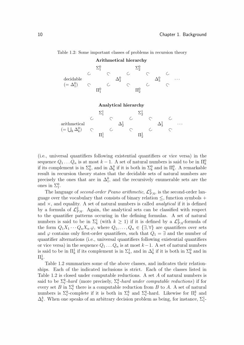
Table 1.2: Some important classes of problems in recursion theory

Arithmetical hierarchy

Σ01 Σ0

2

⊂ ⊂ ⊂ ⊂ ⊂decidable ∆0

2 ∆03 · · ·

(= ∆01)

⊂ ⊂ ⊂ ⊂ ⊂

Π01 Π0

2

Analytical hierarchy

Σ11 Σ1

2

⊂ ⊂ ⊂ ⊂ ⊂arithmetical ∆1

2 ∆13 · · ·

(=⋃

k ∆0k)

⊂ ⊂ ⊂ ⊂ ⊂

Π11 Π1

2

(i.e., universal quantifiers following existential quantifiers or vice versa) in thesequence Q1 . . . Qn is at most k− 1. A set of natural numbers is said to be in Π0

k

if its complement is in Σ0k, and in ∆0

k if it is both in Σ0k and in Π0

k. A remarkableresult in recursion theory states that the decidable sets of natural numbers areprecisely the ones that are in ∆0

1, and the recursively enumerable sets are theones in Σ0

1.

The language of second-order Peano arithmetic, L2PA, is the second-order lan-

guage over the vocabulary that consists of binary relation ≤, function symbols +and ×, and equality. A set of natural numbers is called analytical if it is definedby a formula of L2

PA. Again, the analytical sets can be classified with respectto the quantifier patterns occuring in the defining formulas. A set of naturalnumbers is said to be in Σ1

k (with k ≥ 1) if it is defined by a L2PA-formula of

the form Q1X1 · · ·QnXn.ϕ, where Q1, . . . , Qn ∈ {∃,∀} are quantifiers over setsand ϕ contains only first-order quantifiers, such that Q1 = ∃ and the number ofquantifier alternations (i.e., universal quantifiers following existential quantifiersor vice versa) in the sequence Q1 . . . Qn is at most k−1. A set of natural numbersis said to be in Π1

k if its complement is in Σ1k, and in ∆1

k if it is both in Σ0k and in

Π1k.

Table 1.2 summarizes some of the above classes, and indicates their relation-ships. Each of the indicated inclusions is strict. Each of the classes listed inTable 1.2 is closed under computable reductions. A set A of natural numbers issaid to be Σk

ℓ -hard (more precisely, Σkℓ -hard under computable reductions) if for

every set B in Σkℓ there is a computable reduction from B to A. A set of natural

numbers is Σkℓ -complete if it is both in Σk

ℓ and Σkℓ -hard. Likewise for Πk

ℓ and∆k

ℓ . When one speaks of an arbitrary decision problem as being, for instance, Σ11-


hard, then it is implicitly understood that the instances of the decision problemare coded into natural numbers (using a computable encoding).

The set of (codings of) true Σ11 sentences of arithmetic is itself a Σ1

1-completeset. In fact, this can be strengthened slightly, since the intended interpretationof + and × in (N,≤) can be defined using first-order sentences. In this way, weobtain the following.

1.2.1. Theorem. The existential second order theory of (N,≤) is Σ11-complete.

Another example of a Σ11-hard decision problem, due to Harel [16] is the

recurrent tiling problem, which can be defined as follows. A tile is a tuple t =〈tleft, tright, ttop, tbottom〉 of elements of some set C. A tiling of N × N using a setof tiles T is a function f : N × N → T such that for all n,m ∈ N, f(n,m)right =f(n + 1,m)bottom and f(n,m)top = f(n,m + 1)bottom. Now, the recurrent tilingproblem is the following problem:

given a finite set of tiles T and a designated tile t ∈ T , is there a tilingf of N × N using T such that f(n, 0) = t for infinitely many n ∈ N?

1.2.2. Theorem ([16]). The recurrent tiling problem is Σ11-complete.

Here is an example of a decision problem that is not analytical.

1.2.3. Theorem. Satisfiability of monadic second order formulas over the sig-nature consisting of a single binary relation is highly undecidable, and in fact notanalytical.

Proof: There is a computable satisfiability-preserving translation from arbitrarysecond-order formulas to monadic second order formulas in one binary relationsymbol [18]. By a standard recursion theoretic argument, using the fact that themodel (N,≤,+,×) is defined up to isomorphism by a second order formula, theclass of satisfiable second-order formulas is not analytical (cf. [10]). The resultfollows. 2

Chapter 2

Modal logic

This chapter serves two purposes. Firstly, it reviews the basic notions and resultsof modal logic, from a model theoretic perspective. Secondly, we prove the follow-ing new results: non-recursive enumerability of the first-order formulas preservedunder ultrafilter extensions, an improvement of a general interpolation result formodal logics, and some results concernings hallow modal formulas (i.e., modalformulas in which no occurence of a proposition letter is in the scope of morethan one modal operator).

2.1 Syntax and semantics

We will assume a countably infinite set of proposition letters prop and a finite setof (unary) modalities mod.1 A Kripke frame is a pair F = (W, (R3)3∈mod), whereW is a set, called the domain of F, and each R3 is a binary relation over W . Theelements of the domain of a frame are often called worlds, states, points, nodes,or simply elements. The relations R3 are often called accessibility relations. AKripke model is a pair (F, V ), where F is a Kripke frame, and V : prop → ℘(W )is a valuation for F, i.e., a function that assigns to each proposition letter a subsetof the domain of F. We will often drop the qualification “Kripke”, and simplytalk about frames and models.

The basic modal language M is a language that is used for describing modelsand frames. Its formulas are given by the following recursive definition.

ϕ ::= ⊤ | p | ¬ϕ | ϕ ∧ ψ | 3ϕ

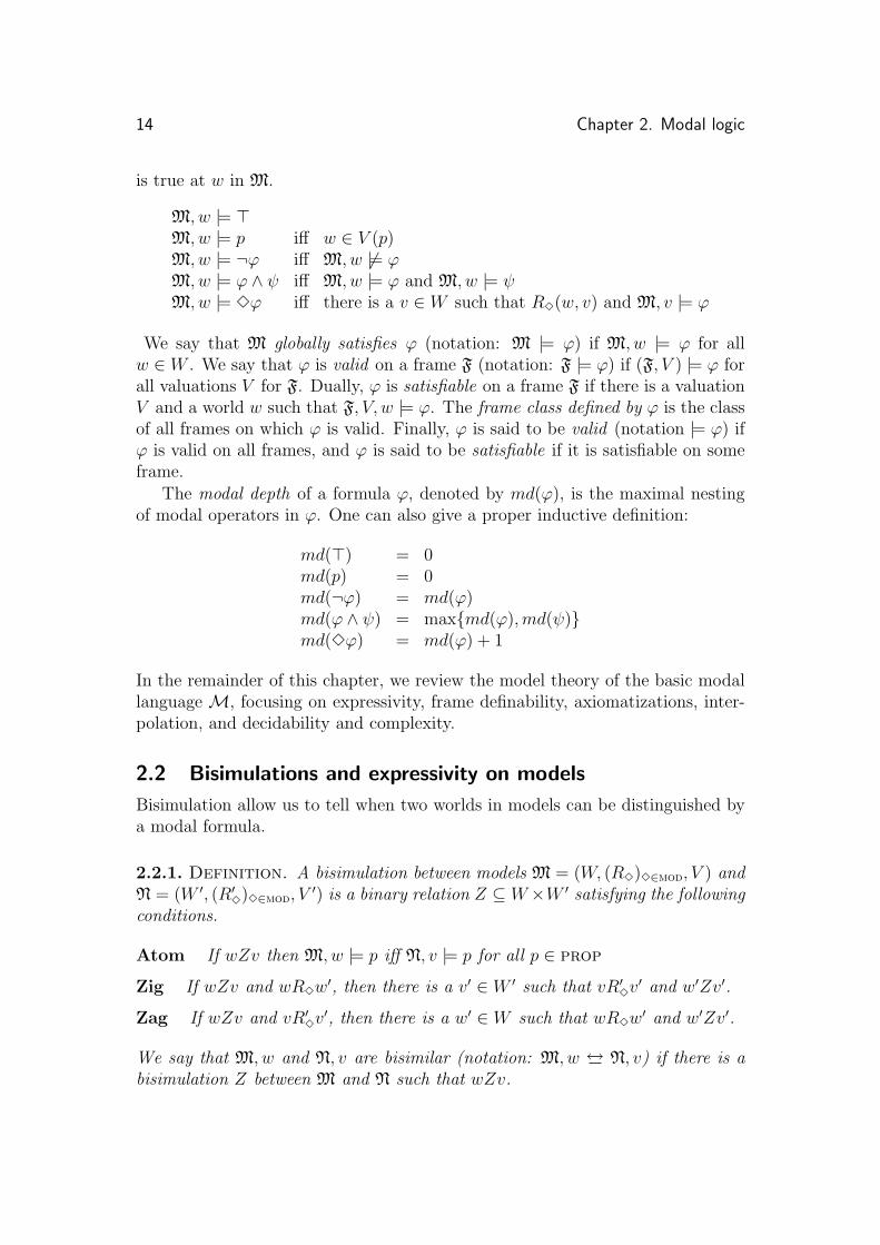
The other connectives, such as 2, will be considered shorthand notations. Givena model M = (W, (R3)3∈mod, V ), a world w ∈ W and a modal formula ϕ, truthor falsity of ϕ at w in M is defined as follows, where M, w |= ϕ expresses that ϕ

1In most parts of this thesis, we restrict attention to a finite set of unary modalities. This isonly for presentational reasons, and all results we present can be generalized to infinitely manymodalities and k-ary modalities (k ≥ 0).

13

14 Chapter 2. Modal logic

is true at w in M.

M, w |= ⊤M, w |= p iff w ∈ V (p)M, w |= ¬ϕ iff M, w 6|= ϕM, w |= ϕ ∧ ψ iff M, w |= ϕ and M, w |= ψM, w |= 3ϕ iff there is a v ∈ W such that R3(w, v) and M, v |= ϕ

We say that M globally satisfies ϕ (notation: M |= ϕ) if M, w |= ϕ for allw ∈ W . We say that ϕ is valid on a frame F (notation: F |= ϕ) if (F, V ) |= ϕ forall valuations V for F. Dually, ϕ is satisfiable on a frame F if there is a valuationV and a world w such that F, V, w |= ϕ. The frame class defined by ϕ is the classof all frames on which ϕ is valid. Finally, ϕ is said to be valid (notation |= ϕ) ifϕ is valid on all frames, and ϕ is said to be satisfiable if it is satisfiable on someframe.

The modal depth of a formula ϕ, denoted by md(ϕ), is the maximal nestingof modal operators in ϕ. One can also give a proper inductive definition:

md(⊤) = 0md(p) = 0md(¬ϕ) = md(ϕ)md(ϕ ∧ ψ) = max{md(ϕ),md(ψ)}md(3ϕ) = md(ϕ) + 1

In the remainder of this chapter, we review the model theory of the basic modallanguage M, focusing on expressivity, frame definability, axiomatizations, inter-polation, and decidability and complexity.

2.2 Bisimulations and expressivity on models

Bisimulation allow us to tell when two worlds in models can be distinguished bya modal formula.

2.2.1. Definition. A bisimulation between models M = (W, (R3)3∈mod, V ) andN = (W ′, (R′

3)3∈mod, V

′) is a binary relation Z ⊆ W×W ′ satisfying the followingconditions.

Atom If wZv then M, w |= p iff N, v |= p for all p ∈ prop

Zig If wZv and wR3w′, then there is a v′ ∈ W ′ such that vR′

3v′ and w′Zv′.

Zag If wZv and vR′3v′, then there is a w′ ∈ W such that wR3w

′ and w′Zv′.

We say that M, w and N, v are bisimilar (notation: M, w ↔ N, v) if there is abisimulation Z between M and N such that wZv.

2.2. Bisimulations and expressivity on models 15

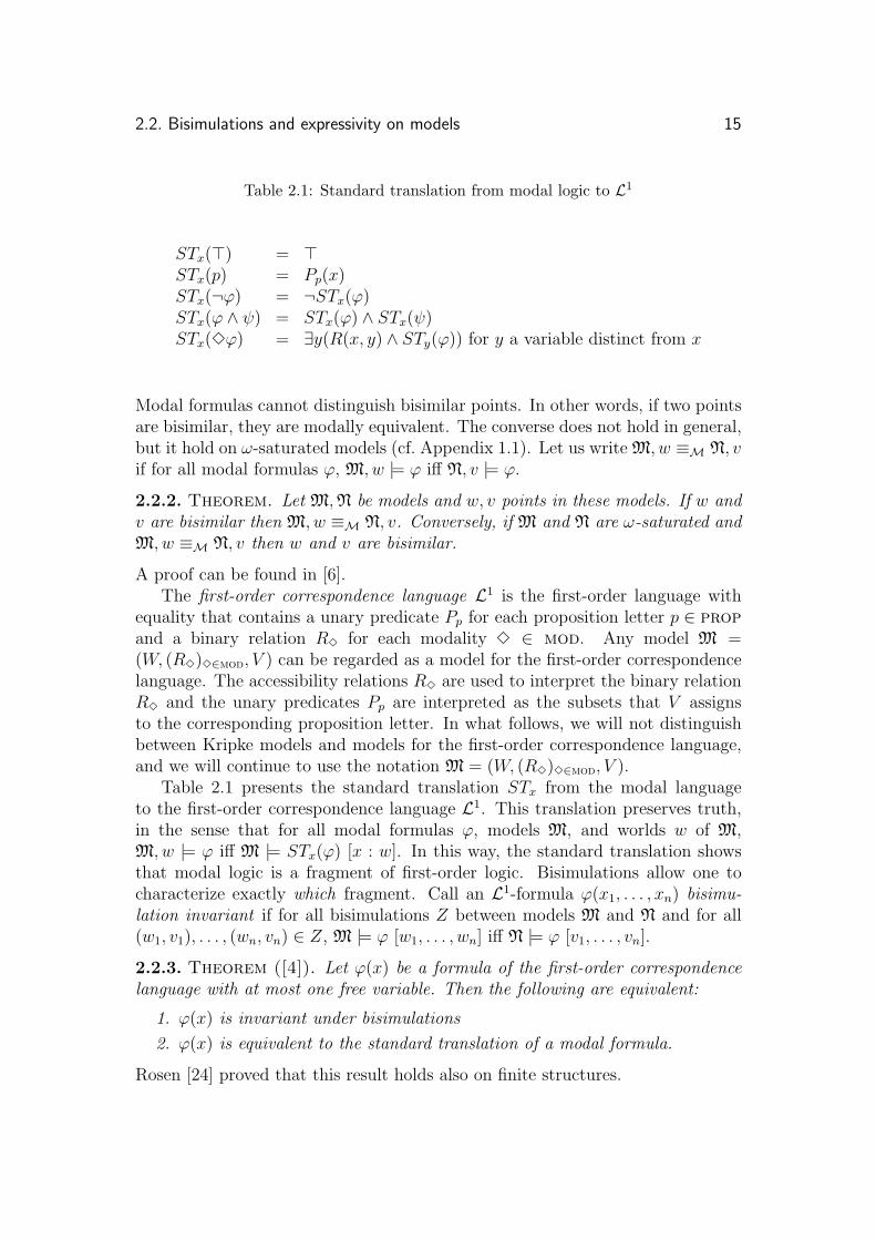
Table 2.1: Standard translation from modal logic to L1

STx(⊤) = ⊤STx(p) = Pp(x)STx(¬ϕ) = ¬STx(ϕ)STx(ϕ ∧ ψ) = STx(ϕ) ∧ STx(ψ)STx(3ϕ) = ∃y(R(x, y) ∧ STy(ϕ)) for y a variable distinct from x

Modal formulas cannot distinguish bisimilar points. In other words, if two pointsare bisimilar, they are modally equivalent. The converse does not hold in general,but it hold on ω-saturated models (cf. Appendix 1.1). Let us write M, w ≡M N, vif for all modal formulas ϕ, M, w |= ϕ iff N, v |= ϕ.

2.2.2. Theorem. Let M,N be models and w, v points in these models. If w andv are bisimilar then M, w ≡M N, v. Conversely, if M and N are ω-saturated andM, w ≡M N, v then w and v are bisimilar.

A proof can be found in [6].The first-order correspondence language L1 is the first-order language with

equality that contains a unary predicate Pp for each proposition letter p ∈ propand a binary relation R3 for each modality 3 ∈ mod. Any model M =(W, (R3)3∈mod, V ) can be regarded as a model for the first-order correspondencelanguage. The accessibility relations R3 are used to interpret the binary relationR3 and the unary predicates Pp are interpreted as the subsets that V assignsto the corresponding proposition letter. In what follows, we will not distinguishbetween Kripke models and models for the first-order correspondence language,and we will continue to use the notation M = (W, (R3)3∈mod, V ).

Table 2.1 presents the standard translation STx from the modal languageto the first-order correspondence language L1. This translation preserves truth,in the sense that for all modal formulas ϕ, models M, and worlds w of M,M, w |= ϕ iff M |= STx(ϕ) [x : w]. In this way, the standard translation showsthat modal logic is a fragment of first-order logic. Bisimulations allow one tocharacterize exactly which fragment. Call an L1-formula ϕ(x1, . . . , xn) bisimu-lation invariant if for all bisimulations Z between models M and N and for all(w1, v1), . . . , (wn, vn) ∈ Z, M |= ϕ [w1, . . . , wn] iff N |= ϕ [v1, . . . , vn].

2.2.3. Theorem ([4]). Let ϕ(x) be a formula of the first-order correspondencelanguage with at most one free variable. Then the following are equivalent:

1. ϕ(x) is invariant under bisimulations

2. ϕ(x) is equivalent to the standard translation of a modal formula.

Rosen [24] proved that this result holds also on finite structures.


2.3 Frame definability

When interpreted on frames, modal formulas express second order frame condi-tions. For instance, the modal formula p → 3p expresses the frame condition∀x.∀P.(Px → ∃y.(Rxy ∧ Py)). At it happens, this particular second order for-mula is equivalent to the first-order formula ∀x.Rxx. However, this is in generalnot the case. For instance, the modal formula 23p → 32p expresses a framecondition that is not definable by first-order formulas.

To be a little more precise, given a set of modal formulas Σ, the frame classdefined by Σ is the class of all frames on which each formula in Σ is valid. Aframe class is modally definable if there is a set of modal formulas that defines it.A frame class is elementary if it is defined by a sentence of the first order framecorrespondence language L1

fr, which is the first-order language with equality andbinary relation symbol for each modality.2

In this section, we discuss a number of result concerning the relationshipbetween modally definable frame classes and elementary frame classes. First,we will consider model theoretic characterizations. Then, we will review someattempts at syntactic characterizations.

Model theoretic characterizations

A famous result due to Goldblatt and Thomason characterizes the modally de-finable elementary frame classes in terms of four operations on frames.

2.3.1. Definition (Generated subframe). A frame F = (W, (R3)3∈mod) isa generated subframe of a frame G = (W ′, (R′

3)3∈mod) if W ⊆ W ′ and for all

(w, v) ∈ R′3

(3 ∈ mod), if w ∈ W then v ∈ W .

2.3.2. Definition (Disjoint union). Let Fi = (Wi, (Ri3)3∈mod) (i ∈ I) be a

set of frames with disjoint domains. The disjoint union of these frames, denotedby

⊎

i∈I Fi is the frame (⋃

i∈I Wi, (⋃

i∈I Ri3)3∈mod).

2.3.3. Definition (Bounded morphism). A bounded morphism from a frameF = (W, (R3)3∈mod) to a frame G = (W ′, (R′

3)3∈mod) is a function f : W → W ′

satisfying the following conditions.

forth for all w, v ∈ W and 3 ∈ mod, if R3(w, v) then R′3(f(w), f(v))

back for all w ∈ W , v ∈ W ′ and 3 ∈ mod, if R′3(f(w), v) then there is a u ∈ W

such that R3(w, u) and f(u) = v.

If there is a surjective bounded morphism from F to G, then we say that G is abounded morphic image of F.

2Note that, in the literature, a class is sometimes called elementary if it is defined by a setof first-order formulas. Here, we call a class elementary if it is defined by a single first-ordersentence.

2.3. Frame definability 17

In order to formulate the fourth operation on frames, we need to introduce a pieceof notation. Given a frame F = (W, (R3)3∈mod), X ⊆ W and 3 ∈ mod, we willwrite m3(X) for the set {w ∈ W | ∃v ∈ X.wR3v}. In other words, m3(X) is theset of 3-predecessors of elements of X.

2.3.4. Definition (Ultrafilter extension). Given a frame F =(W, (R3)3∈mod), the ultrafilter extension of F, denoted by ueF, is the frame(Uf(W ), (Rue

3)3∈mod), where Uf(W ) is the set of ultrafilters over W (cf. Appendix

1.1), and for u, v ∈ Uf(W ), Rue

3(u, v) iff for all X ∈ v, m3(X) ∈ u.

Every modally definable frame class is closed under disjoint unions, generatedsubframes and bounded morphic images. Furthermore, modally definable frameclasses reflect ultrafilter extensions, meaning that whenever the ultrafilter exten-sion of a frame is in the class, then the frame itself is in the class. Goldblattand Thomason proved that the converse holds with respect to elementary frameclasses.

2.3.5. Theorem (Goldblatt-Thomason[12]). An elementary frame class ismodally definable iff it is closed under generated subframes, disjoint unions andbounded morphic images, and reflects ultrafilter extensions.

This tells us which elementary frame classes are modally definable. The oppositequestion, i.e., which modally definable frame classes are elementary, was answeredby Van Benthem.

2.3.6. Theorem ([3]). Let K be any modally definable frame class. The follow-ing are equivalent:

1. K is elementary

2. K is defined by a set of first-order sentences

3. K is closed under elementary equivalence

4. K is closed under ultrapowers.

Syntactic characterizations

The above results do not tell us which modal formulas define an elementary frameclass, nor which first-order formulas define a modally definable frame class.

As we will soon see (cf. Theorem 2.6.5), the problem whether a given modalformula defines an elementary frame class is highly undecidable. This implies thata syntactic characterization of the form “a modal formula defines an elementaryclass iff it is equivalent to a formula of the form X ” with X a decidable class offormulas cannot be obtained. However, this still leaves open the question whethersuch a characterization exists if equivalent is replaced by frame-equivalent.

An important sufficient condition for elementarity was proved by Sahlqvist[25] and Van Benthem [4].


2.3.7. Definition (Sahlqvist formulas). A modal formula is positive(negative) if every occurrence of a proposition letter is under the scope of aneven (odd) number of negation signs.

A Sahlqvist antecedent is a formula built up from ⊤,⊥, boxed atoms of theform 21 · · ·2np (n ≥ 0), and negative formulas using conjunction, disjunctionand diamonds.

A Sahlqvist implication is a formula of the form ϕ→ ψ, where ϕ is a Sahlqvistantecedent and ψ is positive.

A Sahlqvist formula is a formula that is obtained from Sahlvist implicationsby applying boxes and conjunction, and by applying disjunctions between formulasthat do not share any proposition letters.

2.3.8. Theorem ([25, 4]). Every Sahlqvist formula defines an elementary classof frames.

Likewise, Van Benthem [4] has shown that every modal formula that has modaldepth at most one defines an elementary class of frames. Axioms of modal depthat most one were first considered by Lewis [21]. Van Benthem’s result may beimproved slightly, by considering the following class of formulas.

2.3.9. Definition (Shallow formulas). A modal formula is shallow if ev-ery occurrence of a proposition letter is in the scope of at most one modal operator.

2.3.10. Theorem. Every shallow formula defines an elementary class of frames.

Proof: The proof will be given in Section 2.4. 2

Typical examples of shallow modal formulas are p → 3p, 3p → 2p and 31p →32p. Furthermore, every closed formula (i.e., formula containing no propositionletters) is shallow. The formula 21(p∨ q) → 32(p∧ q) is an example of a shallowformula that is not a Sahlqvist formula.

Incidentally, correspondence results like these might also be obtained for lan-guages other than the first-order correspondence language. Recently, [5] and[14] have independently found a generalization of the class of Sahlqvist formulas,with the property that every generalized Sahlqvist formula has a correspondentin LFP(FO), which is the extension of first-order logic with least fixed point op-erators. By results of [1], there are modal formulas that have no correspondentin LFP(FO), not even with respect to finite frames.

Next, let us address the question which first-order formulas define modally defin-able frame conditions. Again, no complete syntactic characterization is known.

Let a p-formula be a first-order formula obtained from atomic formulas (in-cluding equality statements) using conjunction, disjunction, existential and uni-versal quantifiers, and bounded universal quantifiers of the form ∀x(Rtx→ ·). A

2.4. Completeness via general frames 19

p-sentence is a p-formula that is a sentence. An inductive argument shows thatp-sentences are preserved under taking images of bounded morphisms. In fact,the converse holds as well, modulo logical equivalence.

2.3.11. Theorem (Van Benthem [4]). A first-order sentence ϕ is preservedunder surjective bounded morphisms iff ϕ is equivalent to a p-sentence.

It follows that if a first-order sentence defines a modally definable frame class,then it is equivalent to a p-sentence. We can improve this a bit further. Let apositive restricted formula be a first-order formula built up from ⊥ and atomicformulas, using conjunction, disjunction, and restricted quantification of the from∃y.(Rxy ∧ ·) and ∀y.(Rxy → ·), where x and y are distinct variables.

2.3.12. Theorem (Van Benthem [4]). A first-order sentence ϕ is preservedunder surjective bounded morphisms, generated subframes and disjoint unions iffϕ is equivalent to ∀x.ψ(x), for some positive restricted formula ψ(x).

Again, it follows that if a first-order sentence defines a modally definable frameclass, it is equivalent to a sentence of the given form. What remains in orderto obtain a complete characterization is to characterize anti-preservation underultrafilter extensions. It is possible to give a preservation result similar to theabove, that characterizes the first-order sentences (anti-)preserved under ultrafil-ter extensions? The answer is No.

2.3.13. Theorem. Preservation of first-order formulas under ultrafilter exten-sions is Π1

1-hard.

In particular, it follows that the first-order sentences (anti-)preserved underultrafilter extensions are not recursively enumerable, and cannot be characterizedby means of a preservation theorem.

2.4 Completeness via general frames

Given a frame class K, one would like to describe the set of modal formulas valid onK (“the modal logic of K”). For the class of all frames, the axioms and inferencesrules given in Table 2.2 constitute a sound and complete axiomatization. We willrefer to this axiomatization as KM. We will write ⊢KM

ϕ if ϕ is derivable in KM.

2.4.1. Theorem (Basic Completeness). For all modal formulas ϕ, |= ϕ iff⊢KM

ϕ.

Thus, KM axiomatizes the set of modal formulas valid on the class of all frames.In order to axiomatize more restricted frame classes, extra axioms (or rules) mustbe added to KM. For any set Σ of modal formulas, we will use KMΣ to denotethe axiomatization obtained by adding all formulas in Σ as axioms to KM. One


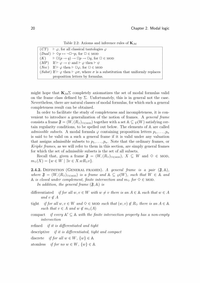
Table 2.2: Axioms and inference rules of KM

(CT ) ⊢ ϕ, for all classical tautologies ϕ(Dual ) ⊢ 3p↔ ¬2¬p, for 2 ∈ mod(K ) ⊢ 2(p→ q) → 2p→ 2q, for 2 ∈ mod(MP ) If ⊢ ϕ→ ψ and ⊢ ϕ then ⊢ ψ(Nec ) If ⊢ ϕ then ⊢ 2ϕ, for 2 ∈ mod(Subst ) If ⊢ ϕ then ⊢ ϕσ, where σ is a substitution that uniformly replaces

proposition letters by formulas.

might hope that KMΣ completely axiomatizes the set of modal formulas validon the frame class defined by Σ. Unfortunately, this is in general not the case.Nevertheless, there are natural classes of modal formulas, for which such a generalcompleteness result can be obtained.

In order to facilitate the study of completeness and incompleteness, it is con-venient to introduce a generalization of the notion of frames. A general frameconsists a frame F = (W, (R3)3∈mod) together with a set A ⊆ ℘(W ) satisfying cer-tain regularity conditions, to be spelled out below. The elements of A are calledadmissible subsets. A modal formula ϕ containing proposition letters p1, . . . , pn

is said to be valid on a such a general frame if it is valid under any valuationthat assigns admissible subsets to p1, . . . , pn. Note that the ordinary frames, orKripke frames, as we will refer to them in this section, are simply general framesfor which the set of admissible subsets is the set of all subsets.

Recall that, given a frame F = (W, (R3)3∈mod), X ⊆ W and 3 ∈ mod,m3(X) = {w ∈ W | ∃v ∈ X.wR3v}.

2.4.2. Definition (General frames). A general frame is a pair (F,A),where F = (W, (R3)3∈mod) is a frame and A ⊆ ℘(W ), such that W ∈ A andA is closed under complement, finite intersection and m3 for 3 ∈ mod.

In addition, the general frame (F,A) is

differentiated if for all w, v ∈ W with w 6= v there is an A ∈ A such that w ∈ Aand v 6∈ A

tight if for all w, v ∈ W and 3 ∈ mod such that (w, v) 6∈ R3 there is an A ∈ A

such that v ∈ A and w 6∈ m3(A)

compact if every A′ ⊆ A with the finite intersection property has a non-empty

intersection

refined if it is differentiated and tight

descriptive if it is differentiated, tight and compact

discrete if for all w ∈ W , {w} ∈ A

atomless if for no w ∈ W , {w} ∈ A

2.4. Completeness via general frames 21

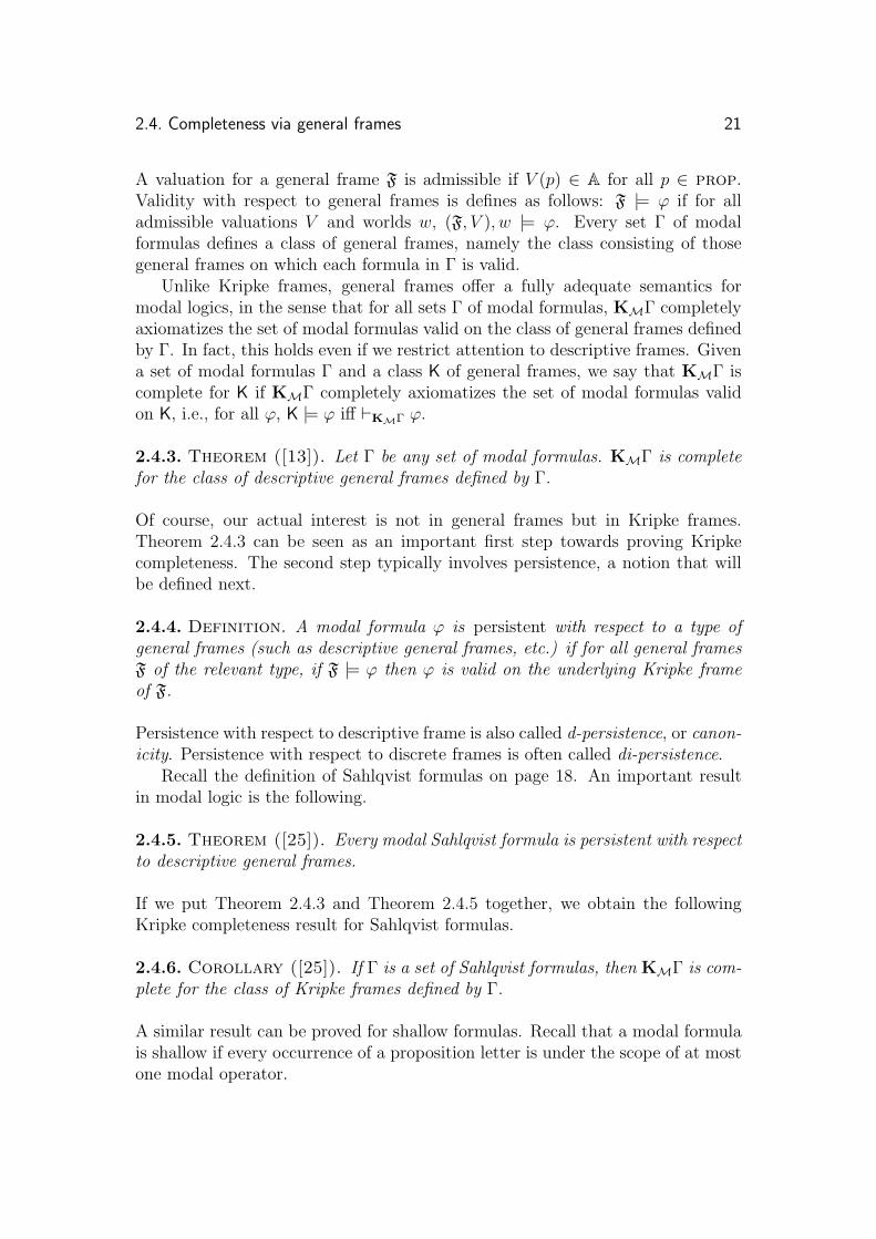
A valuation for a general frame F is admissible if V (p) ∈ A for all p ∈ prop.Validity with respect to general frames is defines as follows: F |= ϕ if for alladmissible valuations V and worlds w, (F, V ), w |= ϕ. Every set Γ of modalformulas defines a class of general frames, namely the class consisting of thosegeneral frames on which each formula in Γ is valid.

Unlike Kripke frames, general frames offer a fully adequate semantics formodal logics, in the sense that for all sets Γ of modal formulas, KMΓ completelyaxiomatizes the set of modal formulas valid on the class of general frames definedby Γ. In fact, this holds even if we restrict attention to descriptive frames. Givena set of modal formulas Γ and a class K of general frames, we say that KMΓ iscomplete for K if KMΓ completely axiomatizes the set of modal formulas validon K, i.e., for all ϕ, K |= ϕ iff ⊢KMΓ ϕ.

2.4.3. Theorem ([13]). Let Γ be any set of modal formulas. KMΓ is completefor the class of descriptive general frames defined by Γ.

Of course, our actual interest is not in general frames but in Kripke frames.Theorem 2.4.3 can be seen as an important first step towards proving Kripkecompleteness. The second step typically involves persistence, a notion that willbe defined next.

2.4.4. Definition. A modal formula ϕ is persistent with respect to a type ofgeneral frames (such as descriptive general frames, etc.) if for all general framesF of the relevant type, if F |= ϕ then ϕ is valid on the underlying Kripke frameof F.

Persistence with respect to descriptive frame is also called d-persistence, or canon-icity. Persistence with respect to discrete frames is often called di-persistence.

Recall the definition of Sahlqvist formulas on page 18. An important resultin modal logic is the following.

2.4.5. Theorem ([25]). Every modal Sahlqvist formula is persistent with respectto descriptive general frames.

If we put Theorem 2.4.3 and Theorem 2.4.5 together, we obtain the followingKripke completeness result for Sahlqvist formulas.

2.4.6. Corollary ([25]). If Γ is a set of Sahlqvist formulas, then KMΓ is com-plete for the class of Kripke frames defined by Γ.

A similar result can be proved for shallow formulas. Recall that a modal formulais shallow if every occurrence of a proposition letter is under the scope of at mostone modal operator.


2.4.7. Theorem. Every shallow formula is persistent with respect to refinedframes, and hence with respect to descriptive frames and with respect to discreteframes.

2.4.8. Corollary. If Γ is a set of shallow formulas, then KMΓ is complete forthe class of Kripke frames defined by Γ.

In fact, combining Theorem 2.4.3, 2.4.5 and 2.4.7, we obtain completeness ofKMΓ for all sets Γ consisting of shallow and/or Sahlqvist formulas.

Incidentally, every modal formula that is persistent with respect to refinedframes defines an elementary frame class [19]. Hence, this also proves Theo-rem 2.3.10.

To finish this section, we briefly consider discrete general frames. Venema [28]proved the following persistence result with respect to discrete general frames.

2.4.9. Definition (Very simple Sahlqvist formulas). A very simpleSahlqvist antecedent is a modal formula built up from ⊤,⊥ and propositionletters using conjunction and diamonds. A very simple Sahlqvist formula isan implication ϕ → ψ, where ϕ is a very simple Sahlqvist antecedent and ψ ispositive.

2.4.10. Theorem ([28]). Every very simple Sahlqvist formula is persistent withrespect to discrete frames.

This by itself does not imply completeness for logics axiomatized by very simpleSahlqvist formulas (even though this follows from Theorem 2.4.5). The reason isthat KMΓ might not be complete for the class of discrete general frames definedby Γ. In other words, there is no analogue of Theorem 2.4.3 for discrete generalframes. Indeed, Venema [28] proved the following strong incompleteness result.

2.4.11. Theorem ([28]). There is a modal formula ϕ such that KM{ϕ} is con-sistent and every general frame on which ϕ is valid is atomless.

It follows that for the relevant formula ϕ, KM{ϕ} is incomplete with respect tothe class of discrete frames defined by ϕ. Incidentally, the formula ϕ used by [28]contains more than one modality. This is necessarily so: an observation due toMakinson implies that, for all uni-modal formulas ϕ, if KM{ϕ} is consistent thenit has a general frame whose domain is a singleton set. Clearly every such generalframe is discrete.

2.5. Interpolation and Beth definability 23

2.5 Interpolation and Beth definability

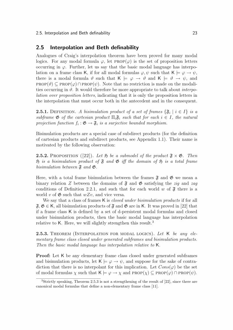
Analogues of Craig’s interpolation theorem have been proved for many modallogics. For any modal formula ϕ, let prop(ϕ) is the set of proposition lettersoccurring in ϕ. Further, let us say that the basic modal language has interpo-lation on a frame class K, if for all modal formulas ϕ, ψ such that K |= ϕ → ψ,there is a modal formula ϑ such that K |= ϕ → ϑ and K |= ϑ → ψ, andprop(ϑ) ⊆ prop(ϕ)∩ prop(ψ). Note that no restriction is made on the modali-ties occurring in ϑ. It would therefore be more appropriate to talk about interpo-lation over proposition letters, indicating that it is only the proposition letters inthe interpolation that must occur both in the antecedent and in the consequent.

2.5.1. Definition. A bisimulation product of a set of frames {Fi | i ∈ I} is asubframe G of the cartesian product ΠiFi such that for each i ∈ I, the naturalprojection function fi : G → Fi is a surjective bounded morphism.

Bisimulation products are a special case of subdirect products (for the definitionof cartesian products and subdirect products, see Appendix 1.1). Their name ismotivated by the following observation:

2.5.2. Proposition ([22]). Let H be a submodel of the product F × G. ThenH is a bisimulation product of F and G iff the domain of H is a total framebisimulation between F and G.

Here, with a total frame bisimulation between the frames F and G we mean abinary relation Z between the domains of F and G satisfying the zig and zagconditions of Definition 2.2.1, and such that for each world w of F there is aworld v of G such that wZv, and vice versa.

We say that a class of frames K is closed under bisimulation products if for allF,G ∈ K, all bisimulation products of F and G are in K. It was proved in [22] thatif a frame class K is defined by a set of d-persistent modal formulas and closedunder bisimulation products, then the basic modal language has interpolationrelative to K. Here, we will slightly strengthen this result.3

2.5.3. Theorem (Interpolation for modal logics). Let K be any ele-mentary frame class closed under generated subframes and bisimulation products.Then the basic modal language has interpolation relative to K.

Proof: Let K be any elementary frame class closed under generated subframesand bisimulation products, let K |= ϕ → ψ, and suppose for the sake of contra-diction that there is no interpolant for this implication. Let Cons(ϕ) be the setof modal formulas χ such that K |= ϕ→ χ and prop(χ) ⊆ prop(ϕ) ∩ prop(ψ).

3Strictly speaking, Theorem 2.5.3 is not a strengthening of the result of [22], since there arecanonical modal formulas that define a non-elementary frame class [11].


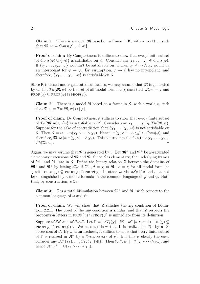
Claim 1: There is a model M based on a frame in K, with a world w, suchthat M, w |= Cons(ϕ) ∪ {¬ψ}.

Proof of claim: By Compactness, it suffices to show that every finite subsetof Cons(ϕ) ∪ {¬ψ} is satisfiable on K. Consider any χ1, . . . , χn ∈ Cons(ϕ).If {χ1, . . . , χn,¬ψ} wouldn’t be satisfiable on K, then χ1 ∧ · · · ∧ χn would bean interpolant for ϕ → ψ. By assumption, ϕ → ψ has no interpolant, andtherefore, {χ1, . . . , χn,¬ψ} is satisfiable on K. ⊣

Since K is closed under generated subframes, we may assume that M is generatedby w. Let Th(M, w) be the set of all modal formulas χ such that M, w |= χ andprop(χ) ⊆ prop(ϕ) ∩ prop(ψ).

Claim 2: There is a model N based on a frame in K, with a world v, suchthat N, v |= Th(M, w) ∪ {ϕ}.

Proof of claim: By Compactness, it suffices to show that every finite subsetof Th(M, w) ∪ {ϕ} is satisfiable on K. Consider any χ1, . . . , χn ∈ Th(M, w).Suppose for the sake of contradiction that {χ1, . . . , χn, ϕ} is not satisfiable onK. Then K |= ϕ → ¬(χ1 ∧ · · · ∧ χn). Hence, ¬(χ1 ∧ · · · ∧ χn) ∈ Cons(ϕ), andtherefore, M, w |= ¬(χ1∧· · ·∧χn). This contradicts the fact that χ1, . . . , χn ∈Th(M, w). ⊣

Again, we may assume that N is generated by v. Let M+ and N+ be ω-saturatedelementary extensions of M and N. Since K is elementary, the underlying framesof M+ and N+ are in K. Define the binary relation Z between the domains ofM+ and N+ by letting dZe if M+, d |= χ ⇔ N+, e |= χ for all modal formulasχ with prop(χ) ⊆ prop(ϕ) ∩ prop(ψ). In other words, dZe if d and e cannotbe distinguished by a modal formula in the common language of ϕ and ψ. Notethat, by construction, wZv.

Claim 3: Z is a total bisimulation between M+ and N+ with respect to thecommon language of ϕ and ψ.

Proof of claim: We will show that Z satisfies the zig condition of Defini-tion 2.2.1. The proof of the zag condition is similar, and that Z respects theproposition letters in prop(ϕ) ∩ prop(ψ) is immediate from its definition.

Suppose w′Zv′ and w′R3w′′. Let Γ = {STx(χ) | M+, w′′ |= χ and prop(χ) ⊆

prop(ϕ) ∩ prop(ψ)}. We need to show that Γ is realized in N+ by a 3-successors of v′. By ω-saturatedness, it suffices to show that every finite subsetof Γ is realized in N+ by a 3-successors of v′. But this is clearly the case:consider any STx(χ1), . . . , STx(χn) ∈ Γ. Then M+, w′ |= 3(χ1 ∧ · · · ∧χn), andhence N+, v′ |= 3(χ1 ∧ · · · ∧ χn).


Finally, it needs to be shown that Z is a total bisimulation. Let w′ ∈ M+. LetΓ = {STx(χ) | M+, w′ |= χ and prop(χ) ⊆ prop(ϕ) ∧ prop(ψ)}. We needto show that Γ is realized in N+. By ω-saturatedness, it suffices to show thatevery finite subset of Γ is realized in N+. Let STx(χ1), . . . , STx(χn) ∈ Γ. Then∃x.(STx(χ1)∧· · ·∧STx(χn)) is true in M+ and therefore also in M (recall thatM+ is an elementary extension of M). Since M is generated by w, there are31, . . . ,3m ∈ mod such that M, w |= 31 · · ·3m(χ1 ∧ · · · ∧ χn). Hence, sincewZv, we have that N, v |= 31 · · ·3m(χ1∧· · ·∧χn). Since N+ is an elementaryextension of N, it follows that N+, v |= 31 · · ·3m(χ1 ∧ · · · ∧ χn). We concludethat there is a point v′ such that N+, v′ |= χ1 ∧ · · · ∧ χn. ⊣

Let F and G be the underlying frames of M+ and N+. Then, in particular, Zis a total frame bisimulation between F and G. Hence, by Proposition 2.5.2,there is a bisimulation product H ∈ K of F and G of which the domain is Z.By the definition of bisimulation products, the natural projections f : H → F

and g : H → G are surjective bounded morphisms. For any proposition letterp ∈ prop(ϕ), let V (p) = {u | M+, f(u) |= p}, and for any proposition letterp ∈ prop(ψ), let V (p) = {u | N+, g(u) |= p}. The properties of Z guaranteethat this V is well-defined for p ∈ prop(ϕ) ∩ prop(ψ). Finally, by a standardargument, the graph of f is a bisimulation between (H, V ) and M+ with respectto prop(ϕ), and the graph of g is a bisimulation between (H, V ) and N+ withrespect to prop(ψ). It follows that (H, V ), 〈w, v〉 |= ϕ∧¬ψ. This contradicts ourinitial assumption that K |= ϕ→ ψ. 2

This result cannot easily be strengthened. An example of an elementary frameclass that is not closed under generated subframes but not under bisimulationproducts, on which the basic modal language lacks interpolation is the class de-fined by 32p→ 23p.4

An example of an elementary frame class closed under bisimulation productsbut not closed under generated subframes on which the basic modal language lacksinterpolation is the class defined by ∀x.(∀y∃z.R1yz → R1xx)∧∀x.(∃y∀z.(R1yz →⊥) → R2xx). It follows from Theorem 2.5.5 below that this first-order sentenceis preserved under taking bisimulation products. Again, an easy bisimulationargument shows that there is no interpolant for the valid implication p∧¬31p→(q → 32q). Note that this implication has an interpolant with global modality,

4To see that the basic modal language lacks interpolation on this frame class, consider thefollowing implication.

(

2(s→ 2(¬p→ r)) ∧ 2(t→ 2(¬p→ ¬r)))

→(

3(s ∧ 2(p→ q)) → 2(t→ 3(p ∧ q)))

This formula is valid on the given frame class, but a simple bisimulation argument shows thatthere is no interpolant. Note that, intuitively, an interpolant would have to express the factthat for every successor x satisfying s and for every successor y satisfying t, x and y have acommon successor satisfying p.


namely E21⊥. Indeed, a relatively straightforward adaptation of the proof ofTheorem 2.5.3 shows that the modal language with global modality, M(E), hasinterpolation on any elementary frame class closed under bisimulation products.

The Beth property

Let |=glo denote the global entailment relation on models, i.e., Σ |=glo ϕ meansthat for all models M, if M globally satisfies all formulas in Σ then M globallysatisfies ϕ. Global entailment relative to a class of frames, denoted by |=glo

K, is

defined similarly. For a set of formulas Σ(p) containing the proposition letter p(and possibly other proposition letters), we say that Σ(p) implicitly defines p,relative to a frame class K, if Σ(p) ∪ Σ(p′) |=glo

Kp ↔ p′. Here, p′ is a proposition

letter not occurring in Σ, and Σ(p′) is the result of replacing all occurrences ofp by p′ in Σ(p). The basic modal language M is said to have the Beth propertyrelative to a frame class K if whenever a set of modal formulas Σ(p) implicitlydefines a proposition letter p relative to K, then there is a modal formula ϑ inwhich p does not occur, such that Σ |=glo

Kp↔ ϑ. The relevant formula ϑ is called

an explicit definition of p, relative to Σ and K.The Beth property is an important property. Intuitively, if a logic has it, this

can be seen as evidence that its syntax and semantics match well. Tarski refersto the Beth property as completeness in the theory of definitions (as opposed tothe theory of deductions).

By a standard argument, we obtain as a corollary of the above interpolationresults the Beth property for the basic modal language, relative to every elemen-tary frame class closed under bisimulation products and generated subframes.

2.5.4. Theorem. If K is a elementary frame class closed under generated sub-frames and bisimulation products, then the basic modal language has the Bethproperty relative to K.

Proof: For ease of presentation we restrict attention to the uni-modal case. Theproof generalizes easily to languages containing more modalities.

Let Σ(p) be any set of modal formulas containing the proposition letter p (andpossibly other proposition letters and nominals), and suppose Σ(p) implicitlydefines the proposition letter p, relative to K. Let p′ be a new proposition letter,and let Σ(p′) be the result of replacing all occurrences of p in Σ by p′. Then,by the definition of implicit definability, Σ(p) ∪ Σ(p′) |=glo

Kp ↔ p′. Let Γ(p) =

{2nϕ | ϕ ∈ Σ(p), n ∈ ω}, and define Γ(p′) similarly.

Claim 1: Γ(p) ∪ Γ(p′) |=K p↔ p′.

Proof of claim: Suppose M, w |= Γ(p) ∪ Γ(p′) for some model M based ona frame in K. Let Mw be the submodel of M generated by w. By closureunder generated subframes, the underlying frame of Mw is also in K. By


construction, Mw globally satisfies Σ(p) and Σ(p′). It follows that Mw globallysatisfies p↔ p′, hence, Mw, w |= p↔ p′, hence M, w |= p↔ p′. ⊣

By compactness, there is a finite subset Γ0 ⊆ Γ such that Γ0(p)∪Γ0(p′) |=K p↔ p′.

It follows that |=K (p ∧∧

Γ0(p)) → (∧

Γ0(p′) → p′). Let ϑ be an interpolant for

this implication. Then the following facts hold.

1. The proposition letters p and p′ do not occur in ϑ.

2. |=K (p ∧∧

Γ0(p)) → ϑ.

3. |=K ϑ → (∧

Γ0(p′) → p′), and hence, by uniform substitution, |=K ϑ →

(∧

Γ0(p) → p).

We conclude that Γ0(p) |=K p↔ ϑ, and hence Σ(p) |=gloKp↔ ϑ. 2

Here is a simple example of an elementary frame class on which the basicmodal language lacks the Beth property. Let K be the class of frames satisfying∃x∀yz.(Ryz ↔ y = x), and let Σ = {p → 2q,¬p → 2¬q}. Clearly, in modelsthat are based on a frame in K and that globally satisfy Σ, q holds at a stateiff p holds at the root, and hence, Σ implicitly defines q in terms of p, relativeto K. However, a simple bisimulation argument shows that there is no explicitdefinition of q in terms of p, relative to Σ and K, in the basic modal language.

Preservation results for bisimulation products

One might ask for a syntactic characterization of the elementary frame proper-ties that are preserved under taking bisimulation products. Such a preservationtheorem can indeed be given. In what follows, we will characterize the first-order formulas that are preserved under bisimulation products, in the form of apreservation theorem. Recall the definition of p-formulas on page 18.

In the following proof we will refer to frames as models (models of the first-order frame correspondence language L1

fr, to be precise). This seems the morenatural choice in the present context, since the theorem concerns first-order for-mulas.

2.5.5. Theorem. A first-order sentence ϕ is preserved under bisimulation prod-ucts iff ϕ is equivalent to a conjunction of sentences of the form ∀~x(ψ → χ),where ψ is a p-formula and χ is either an atomic formula or ⊥.

A similar characterization can be given for the first-order sentences that arepreserved under bisimulation products and generated subframes. Call a strictp-sentence one that contains no unbounded universal quantifiers. In other words:bounded universal quantifiers, unbounded existential quantifiers, positive atoms.

2.5.6. Theorem. A first-order sentence is preserved under bisimulation productsand generated subframes iff it is equivalent to a conjunction of formulas of theform ∀~x(ϕ→ ψ) where ϕ is a strict p-formula and ψ is atomic or ⊥.


2.6 Decidability and complexity

Many decision problems can be formulated in the context of modal logic. Wewill mention a few. The model checking problem: given M, w and ϕ, check ifM, w |= ϕ.

2.6.1. Theorem ([15]). The model checking problem for modal formulas can besolved in polynomial time.

The frame checking problem: given F and ϕ, check if F |= ϕ.

2.6.2. Theorem. The frame checking problem for modal formulas is co-NP-complete.

The modal equivalence problem: given M, w and N, v, check if there is a modalformula that distinguishes w from v.

2.6.3. Theorem ([23]). The modal equivalence problem can be solved in poly-nomial time.

The frame satisfiability problem: given a formula ϕ, check if there is a frame onwhich ϕ is valid.

2.6.4. Theorem. The frame satisfiability problem for modal formulas is highlyundecidable, in fact not analytical.

Proof: By Theorem 1.2.3, the satisfiability problem for monadic second orderformulas in one binary relation is non-analytical. Thomason [27] reduced thisproblem to the following problem:

Given uni-modal formulas ϕ, ψ of the basic modal language, such thatψ is closed (i.e., contains no proposition letters). Does ϕ entail ψ onframes (i.e., is ψ valid on every frame on which ϕ is valid)?

This problem can again be reduced to the frame satisfiability problem: it sufficesto note that, for a modal operator 3 not occurring in ϕ and ψ, ϕ entails ψ onframes iff ϕ∧3¬ψ has no frame (here, we use the fact that ψ is a closed formula).

2

Incidentally, the frame satisfiability problem for uni-modal formulas is triviallydecidable in co-non-deterministic polynomial time, due to the fact that everyframe satisfiable uni-modal formula has a singleton frame.

The elementarity problem: given a formula ϕ, does ϕ define an elementaryframe class?

2.6.5. Theorem. The problem whether a given modal formula defines an ele-mentary frame class is highly undecidable, in fact not analytical.

2.6. Decidability and complexity 29

Proof: Let ϕ be a modal formula, and let 3 be a modal operator not occurringin ϕ. Then ϕ is frame satisfiable iff ϕ ∧ (23p → 32p) is not elementary. Itfollows by Theorem 2.6.4 that the elementarity problem is not analytical. 2

Finally, the decision problem that will receive most attention in this thesis is thesatisfiability problem. For a given frame class K, the problem is to test if a modalformula is satisfiable on K or not. For different classes K, and for different exten-sions of the basic modal language, we will address the question if this problem isdecidable, and if so, what is its complexity.

Let us say that a frame class K has the finite model property if whenevera modal formula is satisfiable on a frame in K, then it is satisfiable on a finiteframe in K. If K has the finite model property, and if membership of a frame withrespect to K can be tested effectively, then the modal formulas that are satisfiableon K can be enumerated: simply enumerate all triples (M, w, ϕ), where M is afinite model, w is a world of M and ϕ is a modal formula, and check for eachsuch triple if M, w |= ϕ and if the underlying frame of M is in K.

Dually, if KM{ϕ} is complete with respect to K, for some ϕ, then we can usethis in order to enumerate the formulas that are not satisfiable with respect toK: simply enumerate all negations of formulas derivable in KM{ϕ}.

If both the satisfiable and the non-satisfiable formulas can be enumerated, thenthe satisfiability problem is decidable: the decision procedure simply performsboth enumerations in parallel, and stops as soon as the input formula occurs inone of the two enumerations. Since every formula is either satisfiable or non-satisfiable, the algorithm will stop after a finite amount of time. Note that whiledecidability might be shown in this way, no concrete bounds on the amount oftime, or space, needed to solve the problem can be derived.

A useful method for proving the decidability and the finite model property isusing filtrations. Let M be a model based on a frame F = (W,R) and let Σ be aset of formulas closed under subformulas. Define an equivalence relation ∼Σ onW such that for every w, v ∈ W :

w ∼Σ v iff for every ψ ∈ Σ, M, w |= ψ iff M, v |= ψ

Denote by [w] the ∼Σ-equivalence class containing w and let W/∼Σbe the set

of all ∼Σ-equivalence classes of W . Define a valuation VΣ on W/∼Σsuch that

VΣ(p) = {[w] | w ∈ V (p)}. The model M/∼Σ= (W/∼Σ

, RΣ, VΣ) is called afiltration of M through Σ if RΣ is a binary relation on W/∼Σ

such that for anyψ ∈ Σ and w ∈ W , M, w |= ψ iff M/∼Σ

, [w] |= ψ. This notion can be generalizedto multi-modal languages as well.

2.6.6. Definition (Filtrations). A frame class K admits filtration if for ev-ery modal formula ϕ there is a finite set of formulas Σϕ containing all subformulasof ϕ, such that whenever M, w |= ϕ and M based on a frame in K, there is afiltration of M over Σϕ whose underlying frame is in K.


We say that K admits polynomial filtration if it admits filtration and the sizeof Σϕ is polynomial in the length of ϕ. We say that K admits simple filtration ifit admits filtration and for every formula ϕ, Σϕ is the set of subformulas of ϕ.

Since |W/∼Σ| ≤ 2|Σ|, if K admits filtration then it has the finite model property.

Since the number of subformulas of ϕ is polynomial in the length of ϕ, everyframe class that admits simple filtration admits polynomial filtration.

2.6.7. Theorem. Let K be any elementary frame class. If K admits polynomialfiltration then satisfiability of modal formulas with respect to K can be decided inNExpTime.

Proof: This can be considered a folklore result.If K admits polynomial filtration, then every satisfiable formula ϕ has a model

whose size can be bounded by an exponential in the length of ϕ. It thereforesuffices to guess such a model and check if it satisfies ϕ and if the underlyingframe is in K. Both of these checks can be performed in polynomial time (notethat the model checking problem for a fixed first order formula can be solved inpolynomial time). 2

Frame classes defined by shallow formulas give us a nice example for the use ofthe filtration method.

2.6.8. Theorem. Every frame class defined by a finite set of shallow modal for-mulas admits polynomial filtration, hence has the finite model property and has asatisfiability problem that can be solved in NExpTime.

Proof: Lewis [21] proved a restricted version of this result, for frame classesdefined by modal formulas with modal depth at most 1. The same proof canbe used to prove our more general result, with a small modification. Let K be aframe class defined by a finite set Γ of shallow modal formulas. For any modalformula ϕ, define Σϕ to be the union of the set of subformulas of ϕ with the set ofclosed subformulas of formulas in Γ (recall that a formula is closed if it containsno proposition letters). Proceeding as in [21] using Σϕ as the filtration set for ϕ,one can construct for every model M based on a frame in K a filtration M′ withrespect to Σϕ, such that the underlying frame of M′ is in K, and ϕ is satisfied atsome world in M′. 2

Bibliography

[1] Jean-Marie Le Bars. The 0-1 law fails for frame satisfiability of proposi-tional modal logic. In Proceedings of the 17th IEEE Symposium on Logic inComputer Science, pages 225–234, 2002.

[2] Johan van Benthem. Logic and Games. Manuscript.

[3] Johan van Benthem. Modal formulas are either elementary or not Σ∆-elementary. Journal of Symbolic Logic, 41:436–438, 1976.

[4] Johan van Benthem. Modal Logic and Classical Logic. Bibliopolis, 1983.

[5] Johan van Benthem. Minimal predicates, fixed points, and definability. Jour-nal of Symbolic Logic, to appear.

[6] Patrick Blackburn, Maarten de Rijke, and Yde Venema. Modal logic. Cam-bridge University Press, Cambridge, UK, 2001.

[7] Egon Borger, Erich Gradel, and Yuri Gurevich. The Classical Decision Prob-lem. Springer-Verlag, 1997.

[8] C.C. Chang and H.J. Keisler. Model Theory. North-Holland PublishingCompany, Amsterdam, 1973.

[9] Kees Doets. Basic Model Theory. Cambridge University Press, 1996.

[10] Kees Doets and Johan van Benthem. Higher-order logic. In D.M. Gabbayand F. Guenthner, editors, Handbook of Philosophical Logic, volume 1, pages275–329. Reidel, 1983.

[11] Kit Fine. Some connections between elementary and modal logic. InS. Kanger, editor, Proceedings of the Third Scandinavian Logic Symposium.North-Holland Publishing Company, 1975.

31

32 Bibliography

[12] R.I. Goldblatt and S.K. Thomason. Axiomatic classes in propositional modallogic. In J. Crossley, editor, Algebra and Logic, pages 163–173. Springer-Verlag, 1974.

[13] Robert I. Goldblatt. Metamathematics of modal logic I. Reports on Mathe-matical Logic, 6:41–78, 1976.

[14] Valentin Goranko and Dimiter Vakarelov. Elementary canonical formulae I:Extending Sahlqvist theorem. Under submission.

[15] Joseph Y. Halpern and Moshe Y. Vardi. Model checking vs. theorem proving:a manifesto. In J.A. Allen, R. Fikes, and E. Sandewall, editors, Principles ofKnowledge Representation and Reasoning: Proc. Second International Con-ference (KR’91), pages 325–334. Morgan Kaufmann, 1991.

[16] David Harel. Recurring dominoes: making the highly undecidable highlyunderstandable. Annals of Discrete Mathematics, 24:51–72, 1985.

[17] Wilfrid Hodges. A Shorter Model Theory. Cambridge University Press, 1993.

[18] Michael Kaminski and Michael Tiomkin. The expressive power of second-order propositional modal logic. Notre Dame Journal of Formal Logic,37(1):35–43, 1996.

[19] A.H. Lachlan. A note on Thomason’s refined structures for tense logics.Theoria, 40:117–120, 1970.

[20] R.E. Ladner, N.A. Lynch, and A.L. Selman. A comparison of polynomialtime reducibilities. Theoretical Computer Science, 1:103–123, 1975.

[21] David Lewis. Intensional logics without iterative axioms. Journal of Philo-sophical Logic, 3:457–466, 1974.

[22] Maarten Marx and Yde Venema. Multi-dimensional Modal Logic. AppliedLogic Series. Kluwer Academic Publishers, 1997.

[23] Robert Paige and Robert Endre Tarjan. Three partition refinement algo-rithms. SIAM Journal on Computing, 16(6):973–989, 1987.

[24] Eric Rosen. Modal logic over finite structures. Journal of Logic, Languageand Information, 6:427–439, 1997.

[25] H. Sahlqvist. Completeness and correspondence in the first and second ordersemantics for modal logic. In S. Kanger, editor, Proceedings of the ThirdScandinavian Logic Symposium, pages 110–143. North-Holland PublishingCompany, 1975.

Bibliography 33

[26] Joseph R. Schoenfield. Recursion Theory, volume 1 of Lecture Notes in Logic.Springer-Verlag, 1993.

[27] S.K. Thomason. Reduction of second-order logic to modal logic. Zeitschriftfur mathemathische Logik und Grundlagen der Mathematik, 21:107–114,1975.

[28] Yde Venema. Derivation rules as anti-axioms in modal logic. Journal ofSymbolic Logic, 58:1003–1034, 1993.

Part II

Topological Semantics for

Modal Logic

The necessary topological definitions have been taken from [Engelking 1977]mostly, while for modal logic we used [Blackburn et al. 2001] as the domi-nating reference.

1.1 Preliminaries

We will define topological semantics for modal logic and present the sound-ness result in this section.First of all, let us specify what kind of structure is a topological space.

Definition 1.1.1 A Topological Space T = (X, τ) is a set X with a collec-tion of its subsets τ satisfying the following:

T1 ∅ ∈ τ and X ∈ τ ,

T2 If O1 ∈ τ and O2 ∈ τ then O1 ∩O2 ∈ τ ,

T3 If Oi ∈ τ for all i ∈ I, with I some index set, then⋃i∈IOi ∈ τ .

The elements of τ are called opens. So, the empty set and the universeare opens, opens are closed under finite intersections and under arbitraryunions. If x ∈ O ∈ τ then we say that O is an open neighbourhood of x.Informally, open neighbourhoods of the given point tell us which points are”close” to the chosen one. It is known that the set O ⊆ X is open iff everypoint in O has an open neighbourhood included in O. The universe is the(biggest) open neighbourhood of all of its points. The complements of opensare called closed and with the de Morgan rules in mind, it does not take longto see that arbitrary intersections, as well as finite unions of closed sets areclosed, as are the universe and the empty set. There are many equivalentmeans of defining topological structure on a set (fixing the family of closedsets is one of them) and we will see some further on in this paper, but whatwe said so far is enough to define the topological semantics for the modallanguage with the single box operator.

37

Chapter 1

Topological semantics and completeness

Definition 1.1.2 The basic modal language consists of countable stock ofproposition letters p, p1, p2, .. the constant truth ⊤, boolean connectives ∧,¬and the modal operator 2. Modal formulas are denoted by Greek letters andare built in the following way:

φ ::= pi | ⊤ | φ ∧ ψ | ¬φ | 2φ.

Now we are ready to define topological models for the basic modal lan-guage. The valuation on the topological space will be the function assigninga subset of the topological space to each propositional letter.

Definition 1.1.3 A topological model M is a triple (X, τ, ν) where T =(X, τ) is a topological space and the valuation ν sends propositional lettersto subsets of X. The notation M, x |= φ (or simply x |= φ) will read ”thepoint x of the model M makes the formula φ true”; if A is a subset of X,A |= φ will mean that x |= φ for all x in A. The definition of truth proceedslike this:

x |= pi iff x ∈ ν(pi),x |= ⊤ always,

x |= φ ∧ ψ iff x |= φ and x |= ψ,

x |= ¬φ iff x 6|= φ,

x |= 2φ iff ∃O ∈ τ : x ∈ O |= φ.

The definitions of model validity and the space validity are standard. Inwords the above definition says that if we associate formulas with the setof points making this formula true, then the abstract operations ¬ and ∧become set-theoretic complement and intersection operations respectively.The last part of the truth definition is not that explicit - it says that formula2φ is true at x, just when φ is true at all the nearby points - everywherein some open neighbourhood of x, that is. Taking a closer look, ν(2φ),defined as the set of points making the formula 2φ true, consists of all thepoints having an open neighbourhood O ⊆ ν(φ). This is nothing else butthe interior part of ν(φ) - a topologist will say. More formally, here comesanother definition from general topology:

Definition 1.1.4 For A subset of the topological space, the interior of A,denoted I(A) is the union of all open sets included in A, or, equivalently, thebiggest open subset of A.

38

To make the picture complete, we recall the following proposition from[Engelking 1977]:

Proposition 1.1.5 The point x belongs to I(A) iff there is an open neigh-bourhood O of x such that O ⊆ A.

In the light of the latter definition and proposition, it should be clear thatν(2φ) = I(ν(φ)). So the abstract 2 operator becomes the interior operatorover the subsets of the topological space in our interpretation. We would liketo mention the topological equivalents for other logical connectives definablein our language. It is rather obvious that the boolean connectives obtain theirtraditional set-theoretic meaning, but what is the topological interpretationof the modal 3? A simple derivation shows that ν(3φ) = −I−(ν(φ)) where− stands for set-theoretic complement operation. Recalling that −I(−A)with A subset of the topological space is nothing else then the closure setof A, we conclude ν(3φ) = C(A). Here C denotes the topological closureoperator, assigning to each subset A of the topological space the smallestclosed set containing this subset - the intersection of all closed sets whichextend A, in other words.

Now, we know more about the I and C from general topology - theysatisfy certain conditions. In fact, given the set equipped with the operatorworking on its subsets, imposing the interior- or closureconditions on thisoperator is another way of defining the topological structure on the set. Letus have a look at these conditions and see what they oblige our 2 to be like.

Proposition 1.1.6 Let (X, τ) be any topological space, I and C the interiorand closure operators defined by topology, then the following holds for anysubsets of X:

(I1) I(X) = X (C1) C(∅) = ∅(I2) I(A) ⊆ A (C2) A ⊆ C(A)(I3) I(A ∩B) = I(A) ∩ I(B) (C3) C(A ∪B) = C(A) ∪ C(B)(I4) I(I(A)) = I(A) (C4) C(C(A)) = C(A)

It is not difficult to notice that the conditions (I1),..,(I4) when read with 2

instead of I look like the axioms for the modal system S4! Dually, conditions(C1),..,(C4) look like S4 axioms written with 3. In fact, as we will seeshortly, any topological model makes the modal logic S4 valid, turning S4into the smallest normal modal logic of topological spaces. Let us put allthese in precise mathematical form.

39

Definition 1.1.7 The modal logic S4 is the smallest set of modal formulaswhich contains all the classical tautologies, the following axioms:

(N) 2⊤

(T) 2p→ p

(R) 2(p ∧ q) ↔ 2p ∧ 2q

(4) 2p → 22p and is closed under modus ponens, substitution and mono-tonicity (from φ→ ψ derive 2φ→ 2ψ).

The above axioms are not exactly the standard way of defining S4, butequivalent to it and the best for our present needs they are. We claim thatevery topological space validates all the modal formulas in S4 thus provingthe soundness of S4 with respect to the topological semantics.

Theorem 1.1.8 The theorems of S4 are valid on every topological space.

Proof: That the axioms (N), (T), (R) and (4) are valid on any topologicalspace is an easy observation after comparing to the conditions (I1), (I2), (I3),(I4). That the derivation rules preserve the validity is a trivial exercise. ⊣

McKinsey and Tarski prove even more in [McKinsey and Tarski 1944],namely that S4 is the complete logic of topological spaces. We will approachthis matter in the next section via Kripke completeness for S4.

1.2 Frames and Completeness

In this section we will build the connections between topological and Kripkesemantics. We will consider S4-frames and see that they come in one-to-onecorrespondence with the special class of topological spaces, called Alexan-droff spaces. This correspondence often facilitates some completeness proofs,showing that for the modal logics above S4 the topological semantics is a gen-eralization of the frame semantics. Concluding this section, we will considerthe modal logics S4.1 and S4.2 and see what class of topological spaces theycharacterize.We have seen in the previous section that every topological model is a modelfor S4. This is not the case in Kripke semantics. The frame is validating S4iff the relation on the frame is reflexive and transitive.

40

Definition 1.2.1 The structure F = (W,R) is called a qo-set (quasi-orderedset) if W is a set and R is a reflexive and transitive relation on W .

Such frames are also enough to refute any non-theorem of S4, as it iswell-known.

Proposition 1.2.2 The modal logic S4 is sound and strongly complete withrespect to the class of all qo-sets.

To illustrate the connection with the topological semantics, let us examineupward closed subsets of a qo-frame F = (W,R). The subset A ⊆ W isupward closed, if together with any point w it contains all of its successors:w ∈ A & Rwv ⇒ v ∈ A. It is not difficult to check that an arbitrary union orintersection of upward closed sets is again upward closed. This is sufficientfor upward closed sets to form a topological structure of open sets on W .Of course, the topology obtained in this way is of a special kind - opensbecome closed under arbitrary, rather then finite, intersection. This sort oftopological spaces are known from general topology:

Definition 1.2.3 A topological space is called Alexandroff space (A-space forshort) if either of the following equivalent conditions hold:1. Arbitrary intersections of opens are open.2. Every point has a least open neighbourhood.

The second condition in the above definition opens the way from A-spacesto qo-sets. To define a reflexive-transitive relation on an A-space, we simplysay that Rxy holds iff y is included in the least open neighbourhood of x.Reflexivity of such a relation is immediate, for transitivity note that if y is amember of the least open neighbourhood Ox of x, then Ox becomes an openneighbourhood of y as well and thus includes in itself all the members of theleast open neighbourhood of y. It is worth mentioning that if we perform theA-space-qo-set transformation both ways starting from either one, we willget the initial structure back.

Well then, we have seen how any qo-set becomes an A-space, but whytreat upward closed sets as opens, why not closed sets? They will happilysatisfy the conditions imposed on the collection of closed sets for topology,will they not? The reason lies behind our definition of the interpretation ofmodal formulas. Indeed, the structures of a qo-set and the correspondingA-space are very much the same - just seen through different mathematical

41

glasses, but what about the modal models built on them? Are they the samein any sense? The following theorem sheds light on these questions.

Theorem 1.2.4 Let F = (W,R) be a qo-set and T = (W, τ) correspondingA-space. For any valuation ν on W , for any point w ∈ W and for any modalformula φ, we have:

F , ν, w |= φ iff T , ν, w |= φ.

Proof: The proof goes by induction on the length of φ. The propositionalcase and the case for the boolean connectives are trivial. Recalling that theR-successors of any point constitute precisely the least open neighbourhoodof this point; and that in A-space 2φ is true at a point iff φ is true in theleast open neighbourhood of this point, we observe that F , ν, w |= 2φ iffT , ν, w |= 2φ, which finishes the proof. ⊣

With the help of the latter theorem we can now prove the topologicalcompleteness of S4.

Theorem 1.2.5 S4 is strongly complete with respect to the class of all topo-logical spaces.

Proof: Take any S4-consistent set of formulas Σ. We know that Σ canbe satisfied in a model of which the underlying frame is a qo-set. Take theA-space corresponding to this qo-set, keeping the valuation. This will be atopological model where Σ is satisfied. ⊣

All we have done so far in this section shows that for S4 and its exten-sions topological semantics is more general then Kripke semantics. If themodal logic containing S4 is (strongly) complete with respect to some classof frames (qo-sets, in fact), then this logic is (strongly) complete with respectto the corresponding class of A-spaces. Certainly the most interesting topo-logical spaces fail to have Alexandroff structure (although note that all finitetopological spaces are clearly A-spaces), but we can still exploit A-spaces forcompleteness results. Witness, for example, the following picture: take anyS4-consistent set of formulas Γ; surely Γ defines some class K of topologicalspaces which make all the formulas in Γ valid. If, in addition, S4 + Γ isKripke (strongly) complete, then it will be topologically (strongly) completewith respect to K, or, indeed, with respect to any subclass of K containing

42

enough A-spaces to refute non-theorems of S4+Γ - thanks to theorem 1.2.4.This is quite a general and vague statement, but we are going to illustrate itin the following section.

Before proceeding to the next section though, we would like to addressone interesting question concerning the topological semantics. Namely, isthere a Kripke-incomplete extension of S4, which is topologically complete?In other words, is the topological semantics really more general than theframe semantics, from the completeness point of view? The answer is affir-mative. In [Gerson 1975] the extension of S4 is presented which is completewith respect to the neighbourhood semantics, but incomplete with respectto Kripke semantics. We can prove that for S4 and its extensions, the neigh-bourhood semantics is equivalent to the topological semantics. It follows thatthe example given by Gerson will also work for proving that the topologicalsemantics is strictly more general then the Kripke semantics. By the timeof writing it was not known to us whether or not these facts have alreadyappeared in literature.

1.3 Some more topological completeness

If the topological semantics is more general than Kripke semantics, we couldjust take any of the extensions of S4 known to be Kripke complete andautomatically get their topological completeness, as outlined at the end ofthe previous section. In case we have the extension of S4 axiomatizable withSahlqvist formulas, we would even get strong completeness! More challengingseems the question which topological property will then the logic in questiondefine. We start with investigating the modal system S4.2.

Definition 1.3.1 The modal logic S4.2 is the extension of S4 with the axiom(.2) 32φ→ 23φ.

It is known that the frames for S4.2 are strongly directed, i.e. any twoworlds having a common predecessor must share a successor, too. The for-mula (.2) being in a Sahlqvist form, gives strong Kripke completeness, andtherefore strong topological completeness - with respect to the class of topo-logical spaces characterized by (.2). To describe this class in topologicalterms, we will need the following definition:

Definition 1.3.2 The topological space is extremally disconnected if any ofthe following two equivalent conditions hold:

43

1. The closure of any open is open.2. The closures of any two disjoint opens are disjoint.

Extremally disconnected spaces were defined in [Stone 1937] and havebeen around in general topology ever since. As it appears, (.2) characterizesthe class of extremally disconnected topological spaces. This statement seemsto be known to scholars working in the field. However we could not find theexact reference who first established it. Here is the proof of this fact:

Theorem 1.3.3 S4.2 defines the class of extremally disconnected topologicalspaces.

Proof: That S4 is valid on any topological space is already known, let uscheck that the formula (.2) is valid on a topological space T = (X, τ) iff Tis extremally disconnected.⇒ Suppose T is not extremally disconnected, then there are O1 and O2

open disjoint sets, such that C(O1) ∩ C(O2) 6= ∅. Define the valuation ν insuch a way that ν(p) = O1. As O1 is open, we have that ν(2p) = I(ν(p)) =I(O1) = O1. We also have O2 |= ¬p and by openness of O2 this impliesO2 |= 2¬p. Take x ∈ C(O1) ∩ C(O2). We claim that x 6|= 32p → 23p.Indeed, for any open neighbourhood Ox of x, we know from x ∈ C(O1) thatOx ∩ O1 6= ∅ ⇒ Ox ∩ ν(2p) 6= ∅ ⇒ x |= 32p. Likewise, from x ∈ C(O2)we get Ox ∩ O2 6= ∅ ⇒ Ox ∩ ν(2¬p) 6= ∅ ⇒ x |= 32¬p and this meansx 6|= 23p.⇐ Say T is extremally disconnected and ν is any valuation on it. Weought to prove ν(32φ) ⊆ ν(23φ) for any φ. In other words, we need toshow ν(32φ) ∩ −ν(23φ) = ∅, with − standing for set-theoretic comple-ment. Now, ν(32φ) = CI(ν(φ)) and −ν(23φ) = −IC(ν(φ)) = CI(−ν(φ)).Clearly, I(−ν(φ)) and I(ν(φ)) are disjoint opens and their closures must bedisjoint by extremal disconnectedness of T , hence T |= 32φ → 23φ, forany φ. ⊣

As an easy consequence we obtain that extremally disconnected A-spacesare in one-to-one correspondence with strongly directed Kripke frames!Summarizing all about S4.2 we have accomplished here, we get the following:

Theorem 1.3.4 S4.2 is sound and strongly complete with respect to the classof extremally disconnected topological spaces.

44

Proof: Soundness is the consequence of the previous theorem, for complete-ness we use the Kripke completeness of S4.2. Indeed, any Kripke framevalidating S4.2 gives rise to an A-space which validates S4.2 by theorem1.2.4 and is, thus, extremally disconnected by the previous theorem. Thenany consistent set of modal formulas Σ can be satisfied in the A-space cor-responding to the frame underlying the S4.2-Kripke-model for Σ. ⊣

We were quite lucky with the formula (.2) - it defined a well-known, topo-logically valuable class. Our next example shows that finding the topologi-cally transparent property characterizing the modally defined class of spacesis not always possible. There are plethora of consistent extensions of S4around (uncountably many, even) and no wonder some of them define ratherbizzare topological properties. Nevertheless, if not entirely transparent andimmediate to the intuition, some of the modal formulas still define interestingclasses of spaces. A good example is the McKinsey formula 23φ → 32φ.This formula first appeared in [McKinsey 1945] where the author baptizedthe corresponding extension of S4 as S4.1.

Definition 1.3.5 The modal logic S4.1 is the extension of S4 with the axiom(.1) 23φ→ 32φ.

It is known that in the presence of transitivity the McKinsey formulameans atomicity for frames, i.e. every point sees a reflexive maximum:∀x∃y(Rxy & ∀z(Ryz → y=z)). The topological counterpart of this propertycan be defined in various equivalent ways, giving different intuitive grasp ofwhat (.1) really says spatially. The following definition is inspired by thenotion used in [Esakia 1979] for the analysis of the system S4.1.

Definition 1.3.6 Let T = (X, τ) be a topological space and A ⊆ X its anysubset. Define the frontier set for A to be the set C(A) ∩ C(−A). Call theoperator Fr defined by the equation Fr(A) = C(A) ∩ C(−A) the frontieroperator.Call the topological space atomic if the frontier of any subset has an emptyinterior, i.e. IFr(A) = ∅ for any A.

To say but a bit more, in atomic spaces no open set can be included inthe frontier of some other set. We will demonstrate that (.1) characterizesthe class of atomic spaces.

45

Theorem 1.3.7 S4.1 is the logic of atomic spaces.

Proof: We have to prove that for any T = (X, τ), T |= 23φ → 32φ iff Tatomic.⇒ Say T is not atomic. Then for some A ⊆ X and for some non-emptyopen O ∈ τ we have O = IFr(A). Define the valuation ν on T in such away that ν(p) = A and note that Fr(A) is exactly the set of points making3p∧3¬p true. Then for any point x ∈ O it is clear that x |= 2(3p∧3¬p)which is equivalent to say that x |= ¬(23p → 32p) so we have refuted theMcKinsey formula.⇐ Assume T 6|= 23φ → 32φ. There must be a valuation ν under whichsome point x falsifies the McKinsey formula x 6|= 23φ → 32φ implyingx |= 23φ and x |= ¬32φ. The latter is equivalent to x |= 23¬φ whichtogether with x |= 23φ means that there are open neighbourhoods O1 andO2 of x such that O1 |= 3φ and O2 |= 3¬φ. Then x ∈ O1 ∩O2 |= 3φ∧3¬φand ν(φ) appears to be the set having the frontier with nonempty open sub-set O1 ∩O2, which denies T from being an atomic space. ⊣

For topological strong completeness witness the following:

Theorem 1.3.8 S4.1 is sound and strongly complete with respect to allatomic spaces.

Proof: Soundness follows from the previous theorem, for strong complete-ness we use the analogous result with respect to Kripke frames for S4.1proved in [Lemmon and Scott 1966]. ⊣

While (.2) defined the essential topological property, spaces characterizedby (.1) seem to receive minor attention in the topological literature. Aswe already mentioned, this is likely to happen with the most topologicalproperties defined by modal formulas in the basic language. This is onlyone side of the coin though - taking modal formulas and tackling with thecorresponding topological property to make some spatial sense of it. Anotherapproach would be to take a topologically sensible class and see which modalformulas may describe it. Or indeed, when is a class of topological spacesdefinable at all? What are the conditions to impose on the class of topologicalspaces to be sure that this class can be characterized by a modal formula?We address this issue in the next part of this work.

46

This part deals with the question of space definability. When is a classof topological spaces modally definable? In the case of Kripke semantics theGoldblatt-Thomason theorem has an answer. Something similar for topolog-ical spaces would have been useful. Let us recall this theorem:

Theorem (Goldblatt-Thomason) A class of frames, closed under takingultrafilter extensions, is modally definable, if and only if it is closed underthe formation of bounded morphic images, generated subframes, and disjointunions, and reflects ultrafilter extensions.

In the first part we have defined topological models, translated framestructure into the topological one, but we did not mention which topologicaloperations preserve space validity. The analogs for bounded morphism, gen-erated subframe and disjoint union will be of a major importance in spacedefinability; the first section of this chapter is devoted to developing thiskind of topological tools. In the second section we will prepare some alge-braic apparatus and work out algebraic duality to approach the definability;all of the latter will allow us to prove the topological Goldblatt-Thomasontheorem in the third section, with the help of the new notion of Alexandroffextension, the topological equivalent of ultrafilter extensions for frames.

2.1 Validity preserving operations

We have built the bridge between Kripke frames and Alexandroff spaces inthe first chapter. Certain operations on frames preserve the validity of modalformulas. Such operations - bounded morphisms, generated subframes anddisjoint union, become crucial when dealing with frame definability. Nowonder we need similar notions for the topological semantics and that iswhat we are about to bring in this section.

While we need to rethink in topological terms the notions of boundedmorphism and generated subframe, the formation of disjoint union appearsto have the straightforward topological equivalent. Here is the definition:

47

Chapter 2

Definable Spaces

Definition 2.1.1 For a family of disjoint topological spaces Ti = (Xi, τi),i ∈ I, their topological sum is the topological space T = (X, τ) with X =⋃i∈IXi and τ = {O ∈ X|∀i ∈ I : O ∩Xi ∈ τi}.

It is easy to observe that when restricted to A-spaces, this operation willyield the structure corresponding to the disjoint union of respective frames.This means we are on the right track, and the following theorem, provingthat the topological sum of topological spaces preserves the validity of modalformulas, justifies our choice.

Theorem 2.1.2 Let (Ti)i∈I be a family of disjoint topological spaces and letφ be a modal formula such that Ti |= φ holds for each i ∈ I. Then forT =

⋃i∈I

Ti we have T |= φ.

Proof: Suppose T 6|= φ for the sake of contradiction. This means there is avaluation ν and a point x ∈ X such that T , ν, x 6|= φ. Obviously, x ∈ Xi forsome i ∈ I. Define the valuation νi as described: νi(p) = ν(p)∩Xi. An easyinduction argument shows that:

Ti, νi, xi |= ψ iff T , ν, xi |= ψ,

for all xi ∈ Xi and all modal formulas ψ. This gives the desired contradic-tion, because we get Ti, νi, x 6|= φ. ⊣NB In fact an easy argument shows that the converse holds as well - eachmember of a family of spaces validates some modal formula, if their topolog-ical sum validates this formula.

This already allows us to show that certain topologically interesting prop-erties (or rather, their corresponding classes) are not definable by (sets of)modal formula(s) in the basic modal language. Our examples are connect-edness and compactness.

Definition 2.1.3 For a topological space T = (X, τ) we say that:(i) T is connected if X can not be presented as the union of two disjointopen subsets.(ii) T is compact if any family (Fi)i∈I of closed subsets of X with the finiteintersection property has a non-empty intersection.

48

Connected and compact topological spaces play the starring role in gen-eral topology. Unfortunately, neither of these properties can be defined inour language. Witness the following:

Theorem 2.1.4 The class of connected topological spaces and the class ofcompact topological spaces are not modally definable.

Proof: The following example serves for both reasons: consider countablymany disjoint sets Xi = {i} with the corresponding topologies τi = {∅, Xi},i ∈ I = {1, 2, ..}. These are one-point sets with the only possible topology.All of them are compact (any finite topological space clearly is), and con-nected. If connectedness (compactness) were definable by a modal formulaφ, all Ti = (Xi, τi) would validate φ and, by the preservation of modal va-lidity under the formation of topological sum, so would T =

⋃i∈I

Ti. This

would imply that T is connected (compact), which it is not. To observe why,note that by the definition of topology on the topological sum of spaces, Tis just a countable set equipped with the discrete topology. In other words,the topology is such, that every subset is both open and closed. In par-ticular, every cofinite set is closed. The collection of cofinite sets form afamily of closed sets with the finite intersection property, but their intersec-tion is empty. This shows T is not compact. Any cofinite set different fromthe universe, together with its complement, form a disjoint couple of opensgiving the universe in union. Thus connectedness of T holds wrong as well. ⊣

This is rather unfortunate. We will see how the enriching of the modallanguage with global diamond will help us to define connectedness in thelast chapter of this work, but compactness (being essentially higher-orderproperty) will still remain wild in this sense. We leave this issue till laterand go on to see the topological equivalents for other basic frame operations.Next comes the notion of generated subframe in our agenda. Recall thata generated subframe is based on a subset of a frame which together withany of its members contains all of its successors. But this is exactly whatwe called ”upward closed sets” in the first chapter and we saw that thetopological notion of open subset is the equivalent for that. At least thiswas the case with A-spaces - upward closed sets constituted the topologywhen forming the A-space from a qo-set. The following theorem shows thatopen subspaces of topological spaces inherit the validity of modal formulas

49

thus proving that open subspaces are the right topological substitute for thenotion of generated subframe.

Theorem 2.1.5 Let U be the open subset of the topological space T = (X, τ)and φ be a modal formula. If T |= φ and TU = (U, τU) is the topological spacewith τU = {O ⊆ U |O ∈ τ}, then TU |= φ.

Proof: For any valuation ν on U let ν ′ be any extension of ν to all of X,agreeing with ν on U . We will prove by induction on the length of modalformulas that for any point u ∈ U , any modal formula ψ:

T , ν ′, u |= ψ iff U, ν, u |= ψ,

which readily implies the claim of the theorem.Since the propositional letters and boolean connectives need not any specialcare, consider the case ψ = 2ψ1.⇒ T , ν ′, u |= 2ψ1 means there is an open neighbourhood O of u, such thatT , ν ′, O |= ψ1. By the definiton of topology on U and the induction hypoth-esis, we get U, ν,O∩U |= ψ1 with O∩U the open neighbourhood of u in τU .This means U, ν, u |= 2ψ1.⇐ U, ν, u |= 2ψ1 means there is an open neighbourhood OU of u in U suchthat U, ν,OU |= ψ1. From the definition of τU it follows that OU ∈ τ . Byinduction hypothesis then T , ν ′, OU |= ψ1 with OU open neighbourhood of uin T , which yields T , ν ′, u |= 2ψ1. ⊣

The class of disconnected topological spaces is that of complementingthe class of connected topological spaces. We have shown the latter to bemodally undefinable. The former appears to be undefinable as well. Justconsider the two-point space with discrete topology - it is disconnected, butthe one-point open subspace of it is clearly connected. As open subspacespreserve validity, disconnectedness can not be modally defined. Althoughrecall that we defined modally the special subclass of disconnected spaces -namely the class of extremally disconnected topological structures - in thefirst chapter.

So open subspaces are the topological twins of generated subframes. Thedifference should be mentioned though - in frames, if A is any subset of aframe, there always exists the least upward closed set containing A - theA-generated subframe. This is the case with Alexandroff spaces as well, butnot generally. In the arbitrary topological space we can always take some

50

open subspace surrounding the given subset A, but one can not always finda least open of this kind.

With this correspondence in hand, it is not hard to find out what thetopological notion of bounded morphism should be. Look what a boundedmorphism does with upward closed sets - the forth condition in the defini-tion of a bounded morphism is just a monotonicity requirement saying thatbounded-morphic preimages of the upward closed sets are upward closed. Intopological terms this would mean that preimages of opens are open. Suchmaps are called continuous in general topology:

Definition 2.1.6 The map f : T1 → T2 between topological spaces T1 =(X1, τ1) and T2 = (X2, τ2) is said to be continuous if whenever O2 ⊆ X2 isopen in T2, the set f−1(O2) is open in T1, i.e.:

O2 ∈ τ2 implies f−1(O2) ∈ τ1.

The back condition in the definition of bounded morphism, when slightlyrephrased, is claiming that the images of upward closed sets are upwardclosed. This corresponds to the definition of open maps in topology.

Definition 2.1.7 The map f : T1 → T2 between topological spaces T1 =(X1, τ1) and T2 = (X2, τ2) is called open if it sends open sets to open sets,i.e.:

O1 ∈ τ implies f(O1) ∈ τ2.

A map is called an interior map, if it is both open and continuous.

The latter definition and our earlier remarks suggest interior maps playthe same role in topological semantics as bounded morphisms do in Kripkesemantics. The following theorem proves this suggestion correct.

Theorem 2.1.8 Let T1 = (X1, τ1) be a topological space and f an interiormap from T1 onto T2 = (X2, τ2). For any modal formula φ, T1 |= φ impliesT2 |= φ.

Proof: Again, for any valuation ν2 on T2 define the valuation ν1 as follows:ν1(p) ≡ f−1(ν(p)). We claim for any modal formula ψ and any x ∈ X1 thefollowing holds:

T1, ν1, x |= ψ iff T2, ν2, f(x) |= ψ.

51

This will then yield the desired validity preservation result, exploiting thesurjectiveness of f . The proof proceeds by induction, with propositional andboolean cases straightforward. Assume ψ = 2ψ1:⇒ From T1, ν1, x |= 2ψ1 it follows that T1, ν1, Ux |= ψ1 for some open neigh-bourhood Ux of x. It is by openness of f that we get f(Ux) is an openneighbourhood of f(x). By induction hypothesis, T2, ν2, f(Ux) |= ψ1 and wearrive at T2, ν2, f(x) |= 2ψ1.⇐ Same as above, with f−1 instead of f . The continuity of f ensures f−1(O2)to be open in T1 provided O2 is open in T2. ⊣

We are almost done with finding the topological equivalents for basicvalidity-preserving operations on frames. The only one left is the formationof ultrafilter extension and we will postpone the definition of the analogoustopological construction till the last section of this chapter. Before that, let usput the constructions we have already defined above to work. In particular,our immediate aim is to show that the separation axioms are not definable bythe modal formula. The definitions of higher separation axioms employ someinvolved topological terminology, which we would like to avoid here. Theaxioms T0 and T1 are defined in the last part of the work. For our presentpurposes it is sufficient to know (cf. [Engelking 1977]) that the real linewith its usual topology obeys the separation axioms T0, T 1

2

, T1, T2, T3, T31

2

, T4.Unlucky as it is, none of these separation axioms can be defined by the modalformula, not being preserved under interior maps. Here is the evidence:

Theorem 2.1.9 The separation axioms Ti with i ≤ 4 are not definable inthe basic modal language.

Proof: Consider the interior map from real line with standard topologyto X = {1, 2} equipped with antidiscrete topology, sending rationals to 1and irrationals to 2. It is easy to verify that the reals obey all separationaxioms, while X obeys none. As interior maps preserve the validity, noneof the separation axioms could be defined by a formula in the basic modallanguage. ⊣

Note that this example will also exhibit non-compactness to be modallyundefinable.Again, we can gain a little by enriching the language we are working with,and we address this issue in the third part of the present work, where we will

52

see how nominals can help to define some lower separation axioms.We would like to make a few remarks on the constructions developed in thissection before going on to the next one.

Other topological constructions: In some cases well-known topologicalconstructions give rise to natural interior maps. The validity preservationautomatically transfers to these constructions. As an example we briefly dis-cuss the topological product of spaces and the quotient of the topologicalspace.The product of topological spaces can be defined in two ways. We would liketo avoid bringing in the respective definitions, but in both cases the naturalprojections are interior maps. This means that if the product of topologicalspaces validates some modal formula, then the components must validatethis formula as well. For the quotient of a topological space note that anyequivalence relation defined on the universe of the space determines a quo-tient space with the natural topology on it (so that the natural quotient mapbecomes continuous). Under the (necessary and sufficient) condition that forany open set O the union of all the equivalence classes intersecting with O isopen, the natural quotient map becomes an interior map. This would meanthat whenever the above condition is satisfied for a space and an equivalencerelation on it, and the space validates the modal formula φ, the quotientspace validates φ as well. For the exact definitions of these topological con-structions we refer to [Engelking 1977].

Topological invariance: Say P is a topological property which our modallanguage is powerful enough to express. It is worth mentioning that theresults of this section imply P is invariant for the formation of topologicalsums, open subspaces and interior images. This obvious consequence of theearlier theorems bears topologically interesting insight. Consider, for exam-ple, atomicity. It is straightforward from the modal point of view that beingan atomic space is a topological property which is invariant under topolog-ical sums, open subspaces and interior images. This is easy to establish bydirect topological proof, but still not entirely obvious. Describing invarianceof properties under various topological transformations is the major task ofgeneral topology. For modally definable properties and three basic validity-preserving topological operations the invariance is automatic, witness theearlier theorems of this section. The same holds for extremal disconnected-ness. We will say a bit more about extremal disconnectedness in the last

53

chapter and get back to the topological invariance in the concluding remarkof the thesis.

In the meantime, we are going to proceed to the next section of thischapter. We choose to approach the desired definability result via algebraicmachinery and the next section is devoted to developing such techniques.Let us conclude this section with the remark that when restricted to A-spaces, the topological notions of topological sum, open subspace and interiormap coincide with the frame-theoretic notions of disjoint union, generatedsubframe and bounded morphism respectively, applied on corresponding qo-sets.

2.2 Interior algebras

First introduced by McKinsey and Tarski, Interior Algebras are BAOs withthe topological operator. Actually, the pioneering completeness proof formodal logic has been carried out with the help of Interior Algebras and theirtopological interpretations. Here we repeat some of the basic definitions andprepare the firm grounds to base our definability result upon. An AbstractInterior Algebra is just a boolean algebra with S4-operator, as formally statedbelow:

Definition 2.2.1 An Interior Algebra is a pair (B,2) where B is a booleanalgebra, 2 is an operator, assigning to each element a of B element 2a ∈ B,such that the following holds:

(I1) 2(a ∧ b) = 2a ∧ 2b,

(I2) 2a ≤ a,

(I3) 22a = 2a,

(I4) 2⊤ = ⊤.

An obvious example of such an algebra would be the full set algebra overany topological space, with I operator. Indeed, any set algebra over the topo-logical space, closed under I, will do. Following the route of the celebratedStone Representation Theorem, we can actually embed any abstract InteriorAlgebra into the power set algebra over some topological space. The carrierof the topology, as in the case of boolean algebras, is the set of all ultrafiltersof the algebra. The topology on this set can be defined in various ways,

54

giving rise to different structures. Our aim favours the definition where therepresentation space has an Alexandroff topology. As we will see shortly, thiscan be done in a natural way. Namely, we declare the set of ultrafilters overan abstract Interior Algebra to be open, if it consists of all the ultrafiltersextending some open filter.

Definition 2.2.2 We call a filter F of an interior algebra (B,2) an openfilter if for any a ∈ B we have that a ∈ F implies 2a ∈ F .We call an element a of an interior algebra open, if a = 2a.

Before checking this definition of the topology to be correct, it shouldbe mentioned ahead that the representation space for an interior algebraA we are about to bring turns out to be the A-space obtained from theultrafilter frame of A by declaring upward-closed sets open. This means ournext theorem, although topologically flavoured, is simply building up theultrafilter frame - in topological terms.

Theorem 2.2.3 Any Interior Algebra A = (A,2) is isomorphic to subalge-bra of all subsets of some A-space.

Proof: Consider the set A∗ ≡ Uf(A) of all ultrafilters of A. For arbitraryfilter F of the algebra by F ∗ we will denote the set of all ultrafilters extendingF . In case F is generated by an element a of the algebra, F = {b ∈ A|b ≥ a},it is clear that F ∗ consists of all ultrafilters having a as an element. In thiscase we may also use the notation a∗ ≡ {u ∈ A∗|a ∈ u}.Let O be any open filter, consider the set O∗ of all ultrafilters which extendO. An easy argument shows that the collection of all O∗ will qualify for thebase of topology. Denote the resulting topological space A∗ = (A∗, τ ∗) andcall it the Alexandroff extension of A.To show that τ ∗ is an Alexandroff topology, it suffices to prove that anyultrafilter has the smallest open neighbourhood. Let u be an arbitrarily cho-sen ultrafilter of A, consider the set of all open elements from this ultrafilterO1

u ≡ {o ∈ u|o = 2o}, which is closed under finite meets according to (I1)and thus generates the filter Ou ≡ {a ∈ A|a ≥ o ∈ O1

u} which obviously isan open filter. From the fact that u is an extension of Ou it follows that O∗

u

is an open neighbourhood of u, it is also the smallest such, as all the openfilters contained in u are also contained in Ou.Now consider the sets a∗ = {u ∈ A∗|a ∈ u} for each a ∈ A. By Stone’s

55

representation theorem, family of subsets (a∗)a∈A of A∗ is a boolean algebraisomorphic to A. Now, showing that A is a subalgebra of (℘A∗, I∗), whereI∗ stands for the interior operator defined by τ ∗, boils down to showing that(2a)∗ = I∗a∗ for each a ∈ A:First observe that (2a)∗ is an open set in τ ∗. Indeed, as we already men-tioned, (2a)∗ coincides with the set of all ultrafilters extending the filtergenerated by 2a. This filter is open because 2a ≤ b implies 2a ≤ 2b by (I1)and (I3). The derivation u ∈ (2a)∗ ⇒ 2a ∈ u⇒ a ∈ u⇒ u ∈ a∗ shows that(2a)∗ ⊆ a∗. We thus proved that (2a)∗ is an open set included in a∗. Tocomplete the proof we will show that (2a)∗ is the biggest open set includedin a∗.Indeed, take any open set O ⊆ a∗, from the definition of τ ∗ we retrieveO =

⋃i∈IO∗

i with O∗

i an open filter for each i ∈ I. It is straightforward that

O∗

i ⊆ a∗ for each i ∈ I. This means that an ultrafilter extending Oi mustcontain a and by ultrafilter theorem this is precisely to say a ∈ Oi. Thus2a ∈ Oi by openness of Oi for each i ∈ I, whence O∗

i ⊆ (2a)∗, for eachi ∈ I. But then O =

⋃i∈IO∗

i ⊆ (2a)∗. Since O was the arbitrary open set

included in a∗, we conclude that (2a)∗ is the greatest open contained in a∗.So (2a)∗ = I∗a∗. ⊣

To get a grasp of what the above construction really does, consider thefollowing.

Definition 2.2.4 For an Interior Algebra A = (A,2) define the relation R∗

on A∗ as follows:R∗uv iff v ∈ Ou.

Where Ou denotes the smallest open neighbourhood of u in τ ∗.

We will show now that R∗ coincides with the relation R+ of the ultrafilterframe for A, thus linking the Alexadroff space we have just built with theultrafilter frame of the respective algebra.

Theorem 2.2.5 Let A = (A,2) be any Interior Algebra. The frame (A∗, R∗)coincides with the ultrafilter frame A+ of A.

Proof: Let us first turn A into BAO by means of defining the operator3 ≡ −2− on the boolean algebra A. This is merely another way of looking

56

at A. Now of two arbitrary ultrafilters u and v the following holds:

R∗uv iff 3a ∈ u for all a ∈ v.

This is to say that the relation R∗ coincides with the relation R+ of the ul-trafilter frame of A. The proof is as follows:⇒ Assume R∗uv and for some a ∈ v, 3a 6∈ u. Since u is an ultrafilter−3a ∈ u⇒ −−2−a ∈ u⇒ 2−a ∈ u. 2−a is an open element, recall formthe proof of the previous theorem that v is some extension of the open filterof all open elements from u, therefore 2−a ∈ v and as far as 2−a ≤ −a andv is an ultrafilter, −a ∈ v which contradicts the assumption a ∈ v.⇐ Now let 3a ∈ u hold for all a ∈ v and assume R∗uv fails; then v must lackat least one open element from u, or, putting it more precisely, there existso ∈ u such that o = 2o and o 6∈ v. By the properties of ultrafilters, then,−o ∈ v and by our assumption 3−o ∈ u. An easy verification shows that3−o = −2−−o = −2o = −o, so −o ∈ u and again, we find a contradictionwith o ∈ u. ⊣

To make the picture complete, we just need some duality results con-cerned with homomorphisms and products. In the light of the last theoremwe could just mention that the homomorphism between two interior algebrasgives rise to the bounded morphism between respective ultrafilter frames andthus, the interior map between their Alexandroff extensions (the correspon-dence established in the first chapter). We supply the proof of this fact inthe terms of theorem 2.2.3 for interested reader. First let us define how tolift the homomorphism between algebras to the map between correspondingAlexandroff extensions.

Definition 2.2.6 Let h : A1 → A2 be homomorphism of Interior Algebras.Define h∗ : A∗

2 → A∗

1 as follows:

h∗(u2) = {a1 ∈ A1|h(a1) ∈ u2} .

A simple verification shows that h∗ is defined correctly (it maps ultrafiltersto ultrafilters). Topologically, it also appears an interior map. We prove thisfact below.

Theorem 2.2.7 If h : A1 → A2 is a homomorphism of Interior Algebras,then h∗ : A∗

2 → A∗

1 is an interior map between topological spaces. Addition-ally, if h is injective (surjective) then h∗ is surjective (injective).

57

Proof: h∗ can be easily checked to be sending ultrafilters to ultrafilters, sur-jectively if h is injective and injectively if h is surjective. The only non-trivialpart to prove remains h∗ being interior (that is, open and continuous). Thissuffices to be checked just on the elements of the respective bases (providedwe first establish continuity and then openness), as it is known from generaltopology (cf. [Engelking 1977], section 1.4). Let us proceed towards this aim.To prove the continuity of h∗ consider O∗

1 ∈ τ ∗1 element of the base generatedby the open filter O1 and take h∗−1O∗

1 which consists of all such ultrafilters ofA2 h

∗-images of which contain O1 as a subset, or, in other words, all ultrafil-ters of A2 which contain the set h(O1). Although h(O1) may not be a filter,it is closed under finite meets because O1 was closed under finite meets andh respects the boolean operations. Hence the set of all ultrafilters containingh(O1) will coincide with the set of all ultrafilters containing the smallest filtergenerated by h(O1). This filter is an open filter, because O1 was an openfilter and h respects the 2. So we obtain h∗−1O∗

1 = (h(O1))∗ ∈ τ ∗2 .

For openness of h∗ we take an element of the base of τ2 denoted O∗

2 andconsider the set h∗(O∗

2). A typical representative of this set has the formh∗(u2) where u2 is such that O2 ⊆ u2. Since h∗(u2) = {a1 ∈ A1|h(a1) ∈ u2},it is immediate that h−1(O2) ⊆ h∗(u2). For h is a homomorphism and O2 isan open filter, it follows that h−1(O2) is an open filter of A1 and this meansnothing but h∗(O∗

2) = (h−1(O2))∗ ∈ τ ∗1 .

Concluding this section, we show how to deal with the products of theset interior algebras.

Proposition 2.2.8 Let Ti be the collection of topological spaces indexed withthe set I. Denote by (Ti)∗ the power set algebra over Ti with respective inte-rior operator. (Ti)∗ are clearly interior algebras, and the following holds:

∏

i∈I

(Ti)∗ ∼= (⋃

i∈I

Ti)∗ .

With ∼= standing for IA-isomorphism and⋃

for the topological sum of topo-logical spaces.

Proof: Define the map f :∏i∈I

(Ti)∗ → (⋃i∈I

Ti)∗ as follows:

For (ai)i∈I ∈∏i∈I

(Ti)∗ note that each ai ∈ (Ti)∗ corresponds to the subset

58

Ai ⊆ Ti. Then define f((ai)i∈I) = (⋃i∈IAi)∗. In other words, take the topo-

logical sum of all Ai and send f((ai)i∈I) to corresponding element of InteriorAlgebra of all subsets of

⋃i∈I

Ti. It is a subject of a routine check that f is

an isomorphism of interior algebras. To clarify why f commutes with theinterior operator, note that on the product of algebras interior operator isdefined componentwise; on the topological sum of topological spaces interioroperator also works componentwise. ⊣

2.3 Topological Goldblatt-Thomason theorem

We have exhibited the topological equivalents for basic frame operations ofdisjoint union, generated subframe and bounded morphic image. The fourthcrucial operation on frames is formation of the ultrafilter extension. Westill lack the topological equivalent for that. Since A-spaces are in one-to-one correspondence with S4-frames, such an equivalent should yield theultrafilter extension of corresponding frame when applied to an A-space.But then we already have one implicit candidate that will do this job! Justtake the interior algebra of all subsets of topological space and consider theAlexandroff extension of it - when starting from an A-space, this procedurewill result in the ultrafilter extension for this frame. This entire sectionis the justification of this choice, with application to topological version ofGoldblatt-Thomason theorem.

Definition 2.3.1 For a given topological space T = (X, τ) define its Alexan-droff extension to be the A-space T ∗ ≡ (℘(X)∗, τ ∗) of the interior algebra ofall subsets of X.

In other words, just take the upward-closed set topology on the ultrafilterframe for the power set algebra of T and define the standard valuation on itas follows:

Definition 2.3.2 If M = (T , ν) is a topological model, define the standardvaluation ν∗ on the T ∗ as follows:

u ∈ ν∗(p) iff ν(p) ∈ u.

This definition will help us to show that Alexandroff extension anti-preservesthe modal validity. We could use the relational, rather than topological,

59

structure on T ∗ in the proof, reproducing the analogous result about ultra-filter extension of a frame, but the presented proof is shorter and fits betterin the framework of this chapter.

Theorem 2.3.3 Let T = (X, τ) be a topological space, M = (T , ν) a topo-logical model based on it, T ∗ the Alexandroff extension of T and ν∗ the stan-dard valuation, then the following holds for any modal formula φ:

u ∈ ν∗(φ) iff ν(φ) ∈ u.

Proof: We proceed by induction on the length of φ. The propositional caseis taken care of by the definition of ν∗, the cases of the boolean connectivesare rather obvious, so we only address the modality case. Consider a formulaof 2φ form:⇒ By definition u ∈ ν∗(2φ) means that u has an open neighbourhood (re-strict to the element of the base without loss of generality) O∗

u such thatv |= φ holds for all v ∈ O∗

u. In other words, Ou ⊆ v implies v |= φ. By theinduction hypothesis this can be rephrased as Ou ⊆ v implies ν(φ) ∈ v forall v. This indicates that ν(φ) is an element of Ou, for if ν(φ) 6∈ Ou werethe case, by ultrafilter theorem we could find an ultrafilter extending Ou andstill leaving ν(φ) aside. So ν(φ) ∈ Ou. Hence, Ou being an open filter yieldsI(ν(φ)) ∈ Ou and since u extends Ou, we arrive at I(ν(φ)) ∈ u.⇐ Suppose ν(2φ) ∈ u, this means I(ν(φ)) ∈ u. Consider any ultrafilterv from the smallest open neighbourhood of u. Any such ultrafilter containsall the open elements from u. Thus I(ν(φ)) ∈ v because I(ν(φ)) is an openelement of u. Then I(ν(φ)) ⊆ ν(φ) implies ν(φ) ∈ v. By the inductionhypothesis v ∈ ν∗(φ). As v was arbitrarily chosen from the smallest openneighbourhood of u, we get u ∈ ν∗(2φ). ⊣

We are finally in the position of presenting the main result of this chapter:a topological version of Goldblatt-Thomason theorem about definable classes.

Theorem 2.3.4 (Topological Goldblatt-Thomason) The class K of topo-logical spaces which is closed under formation of Alexandroff extensions ismodally definable iff it is closed under taking opens subspaces, interior im-ages, topological sums and it reflects Alexandroff extensions.

Proof: We only deal with the right to left direction, as the other directionappears trivial given the earlier theorems 2.1.2, 2.1.5, 2.1.8 and 2.3.3.

60

Assume that K is any class of spaces satisfying the conditions of the theoremand let T = (X, τ) be a space validating the modal theory of K, then theInterior Algebra of all subsets of X, denoted T∗, is validating the equationaltheory of algebras corresponding to the spaces from K. Thus by Birkhoff’stheorem, T∗ is isomorphic to HSP of such algebras. So there are algebrasH, S and P and mappings h and s such that:

(1) h : H → T∗ is onto IA-homomorphism.

(2) s : H → S is injective IA-homomorphism.

(3) S =∏i∈I

(Pi)∗ where Pi ∈ K and (Pi)∗ is the IA of all subsets of Pi

for each i ∈ I .

From (3), definition of Alexandroff extension and the proposition 2.2.8we obtain that S = (

⋃i∈I

Pi)∗ and denoting P =⋃i∈I

Pi we get P ∈ K by the

closure under the formation of topological sum. So S = P∗.Now we exploit (2) lifting up s to Alexandroff extensions, and as far as s isinjective IA-homomorphism, we find that s∗ : (P∗)

∗ → H∗ is an onto interiormap. Note that (P∗)

∗ is nothing else but the Alexandroff extension of P andthus belongs to K by the conditions we imposed on this class; but then so isH∗ being the interior image of the space from K. So H∗ ∈ K.Finally we treat (1), again lifting up h to Alexandroff extensions and obtain-ing h∗ : (T∗)

∗ → H∗ where h∗ in now an injective interior map, so h∗((T∗)∗)

is an open subset of H∗ and, by closure conditions, h∗((T∗)∗) ∈ K. Note that

h∗ : (T∗)∗ → h∗((T∗)

∗) is bijective interior map (homeomorphism). This im-plies (T∗)

∗ ∈ K. We just have to mention that (T∗)∗ is simply an Alexandroff

extension of T , so, by K reflecting Alexandroff extensions, (T∗)∗ ∈ K readily

implies desired T ∈ K. ⊣

As an immediate consequence, we get that the class of Alexandroff spaces,obviousely closed under the formation of Alexandroff extensions, is not modallydefinable - it clearly does not reflect Alexandroff extensions!

61

3.1 Enriching the language

As promised in the earlier chapters, we will show in this section how ex-tending the modal language helps us to define some of otherwise undefinabletopological properties/classes. We will consider adding the global modality,the difference operator and nominals. The case with global modality has al-ready been considered in [Shehtman 1999] where connectedness is expressedas well. Let us consider all these options in turn.

Global Modality: Add to the language with topological box operatorthe global modality. We could even view the global box (written A) as aspecial kind of topological box with the fixed antidiscrete1 topology interpre-tation! The global modality combined with the topological one gives rise tothe logic S4 ∗ S5 and the connectedness becomes expressible by the modalformula A(3φ → 2φ) → (Aφ ∨ A¬φ), as shown in [Shehtman 1999]. Wewould like to add that the example displayed in the theorem 2.1.9 still showsnon of the separation axioms can be expressed even in this richer language -interior maps preserve validity here too.

What happens with definability when we add the global diamond to ourlanguage? In the case of Kripke semantics we know that two of the closureconditions in the Goldblatt-Thomason theorem drop out. Namely the closureunder disjoint unions and generated subframes, for those no longer preservethe validity of modal formulas in the enriched language. This of courseimplies that the topological sum and the open subspace do not preserve themodal validity in the language with additional global modalities. However,interior images and Alexandroff extensions still do. We sketch the proofsbelow.

Theorem 3.1.1 Let T1 = (X1, τ1) be a topological space and f an interior

1Antidiscrete topology (also called trivial topology in the literature) consists solely ofempty set and the universe.

62

Chapter 3

Richer Languages

map from T1 onto T2 = (X2, τ2). For any modal formula φ in the languagewith additional global modality, T1 |= φ implies T2 |= φ.

Proof sketch: Note that the mere fact that f is a surjective mapping en-sures that f is still an interior map when we equip X1 and X2 with theantidiscrete topologies. Use the theorem 2.1.8 thinking of A as a topologicalbox with the fixed antidiscrete interpretation. ⊣

Theorem 3.1.2 Let T = (X, τ) be a topological space, M = (T , ν) a topo-logical model based on it, T ∗ the Alexandroff extension of T and ν∗ the stan-dard valuation, then the following holds for any modal formula φ in the modallanguage with additional global modality:

u ∈ ν∗(φ) iff ν(φ) ∈ u.

Proof sketch: Proving by induction on the length of formulas, witness thefollowing chain of equivalent statements: u ∈ ν∗(Aφ) ⇔ ∀v(v ∈ ν∗(φ)) ⇔∀v(ν(φ) ∈ v) ⇔ ν(φ) = X ⇔ ν(Aφ) = X ∈ u. ⊣.

These prove the easy direction of the definability theorem to proved inthe next part of this reader.The difference operator: Enrich the basic modal language with the newdiamond D saying something is true somewhere else. The global diamond isdefinable in this language by the formula Eφ↔ φ∨Dφ. It follows readily thatconnectedness is expressed as well. We can do even better - the separationaxioms T0 and T1 become modally definable. Let us first give the topologicaldefinition of these axioms.

Definition 3.1.3 We say that a topological space T obeys the T0 separationaxiom if for any two distinct points x and y, one of them has an open neigh-bourhood not containing the other.We say that a topological space T obeys the T1 separation axiom if for anytwo distinct points x and y, each of them has an open neighbourhood notcontaining the other.

The following is how the separation axioms T0 and T1 can be defined inthe modal language enriched with the difference operator.

63

Theorem 3.1.4 Consider the basic modal language enriched with the dif-ference operator D and with diamond interpreted as closure operator. Thefollowing two formulas define the T0 and T1 separation axioms respectively:

t0 = Up ∧DUq → 2¬q ∨D(q ∧ 2¬p),

t1 = Up→ A(p↔ 3p).

Where Uφ is defined as φ ∧ ¬Dφ and Aφ is defined φ ∧ ¬D¬φ.

Proof: First recall that Uφ is true at a world x in a model iff φ is true at xand only there.T0 ⇒ t0 Take a T0 topological space T = (X, τ) and any valuation ν on it.If some point x1 makes the antecedent of t0 true, this proves ν(φ) = {x1}and ν(ψ) = {x2} for some x2 6= x1. At least one of the points x1 or x2 hasan open neighbourhood not containing the other one, which is exactly whatthe consequent of t0 needs to be true.t0 ⇒ T0 If T |= t0 then it does so for any valuation and any substitutioninstance of t0. For any two points x1, x2 ∈ X consider the valuation ν(p1) ={x1}, ν(p2) = {x2} and employ x1 |= Up1 ∧DUp2 → 2¬p2 ∨D(p2 ∧ 2¬p1).Antecedent is true (we designed the valuation for it) and the consequent mustbe true as well, which means either x1 |= 2¬p2 or x1 |= D(p2 ∧ 2¬p1). Ifx1 |= 2¬p2 is true, then x1 obtains the open neighbourhood with ¬p2 truethroughout. Thus none of the points in this neighbourhood can be x2. Ifx1 |= D(p2 ∧ 2¬p1) is the case, for some x3 ∈ X we have x3 |= p2 ∧ 2¬p1.Since p2 is only true at x2, from x3 |= p2 we get x3 = x2. Thus x2 |= 2¬p1,which means x2 has an open neighbourhood making ¬p1 true. Hence x2 hasan open neighbourhood disjoint from x1.T1 ⇒ t1 Recall that T1 spaces are precisely those where singletons are closed,or equivalently, where the closure of every point is this point itself. If T issuch a space and ν any valuation on it, consider any point x making theantecedent of t1 true. This means ν(φ) = {x} and by T1 also ν(3φ) = {x}implying that the consequent is true as well.t1 ⇒ T1 If T |= t1 and x ∈ X is any point, take the valuation ν(p) = {x}and exploit x |= Up → A(p ↔ 3p) bearing in mind that x |= Up by thedefinition of ν. We get ν(3p) = {x} = C {x} which is to say T is T1-spacegiven x was arbitrary. ⊣See [de Rijke 1992] for a thorough survey of the modal languages with dif-ference operator. Some aspects are discussed in [Blackburn et al. 2001] also,where a hybrid languages are considered as well.

64

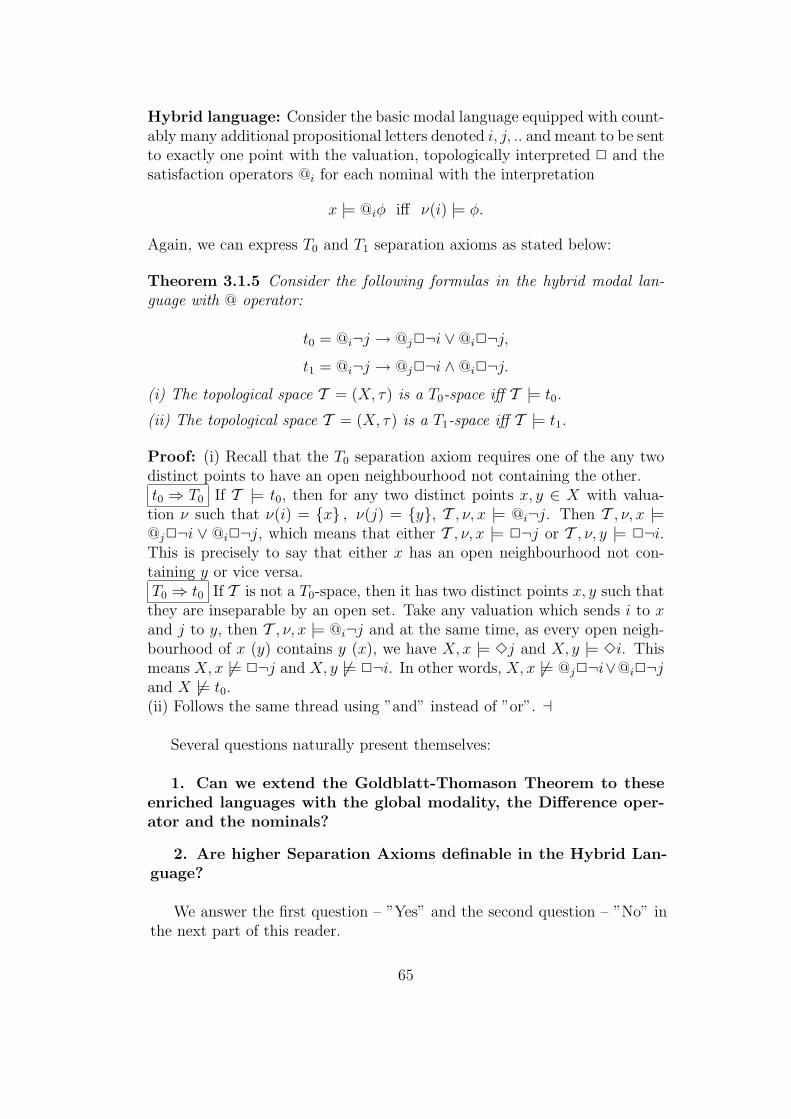
Hybrid language: Consider the basic modal language equipped with count-ably many additional propositional letters denoted i, j, .. and meant to be sentto exactly one point with the valuation, topologically interpreted 2 and thesatisfaction operators @i for each nominal with the interpretation

x |= @iφ iff ν(i) |= φ.

Again, we can express T0 and T1 separation axioms as stated below:

Theorem 3.1.5 Consider the following formulas in the hybrid modal lan-guage with @ operator:

t0 = @i¬j → @j2¬i ∨ @i2¬j,

t1 = @i¬j → @j2¬i ∧ @i2¬j.

(i) The topological space T = (X, τ) is a T0-space iff T |= t0.

(ii) The topological space T = (X, τ) is a T1-space iff T |= t1.

Proof: (i) Recall that the T0 separation axiom requires one of the any twodistinct points to have an open neighbourhood not containing the other.t0 ⇒ T0 If T |= t0, then for any two distinct points x, y ∈ X with valua-tion ν such that ν(i) = {x} , ν(j) = {y}, T , ν, x |= @i¬j. Then T , ν, x |=@j2¬i ∨ @i2¬j, which means that either T , ν, x |= 2¬j or T , ν, y |= 2¬i.This is precisely to say that either x has an open neighbourhood not con-taining y or vice versa.T0 ⇒ t0 If T is not a T0-space, then it has two distinct points x, y such thatthey are inseparable by an open set. Take any valuation which sends i to xand j to y, then T , ν, x |= @i¬j and at the same time, as every open neigh-bourhood of x (y) contains y (x), we have X, x |= 3j and X, y |= 3i. Thismeans X, x 6|= 2¬j and X, y 6|= 2¬i. In other words, X, x 6|= @j2¬i∨@i2¬jand X 6|= t0.(ii) Follows the same thread using ”and” instead of ”or”. ⊣

Several questions naturally present themselves:

1. Can we extend the Goldblatt-Thomason Theorem to theseenriched languages with the global modality, the Difference oper-ator and the nominals?

65

2. Are higher Separation Axioms definable in the Hybrid Lan-guage?

We answer the first question – ”Yes” and the second question – ”No” inthe next part of this reader.

[Aiello and van Benthem 2001] M. Aiello and J. van Benthem, ”Logical pat-terns in space”, D. Barker-Plummer and Etchemendy, J. and Scotto diLuzio, P. and van Benthem, J. (editors), Logic Unleashed: Language, Di-agrams, and Computation, Forthcoming, CSLI Publications, Stanford,2001.

[Aiello et al. 2001] M. Aiello, J. van Benthem, G. Bezhanishvili, Reasoningabout Space: the Modal Way, Manuscript, Univ. Amsterdam and NewMexico, 2001.

[Bezhanishvili and Gehrke 2001] G. Bezhanishvili and M. Gehrke, A NewProof of Completeness of S4 with respect to the Real Line, submitted,2001.

[Blackburn et al. 2001] P. Blackburn, M. de Rijke and Y. Venema, ModalLogic, Cambridge University Press, 2001.

[Engelking 1977] R. Engelking, General Topology, Polish Scientific Publish-ers, Warszawa, 1977.

[Esakia 1979] L. Esakia ”On the theory of modal and superintuitionistic sys-tems”, in Logical Derivation, Moscow, Nauka, 1979, pp. 147-171 (InRussian).

[Gerson 1975] M. Gerson, ”An extension of S4 complete for the neighbour-hood semantics but incomplete for the relational semantics”, Studia Log-ica, 34(1975), pp. 333-342.

[Goldblatt 1980] R. Goldblatt, ”Diodorean Modality in Minkowski Space-time”, Studia Logica, 39(1980), pp. 219-236.

66

Bibliography

[Lemmon and Scott 1966] E. Lemmon and D. Scott, Intentional Logics,Stanford, 1966.

[McKinsey and Tarski 1944] J.C.C. McKinsey and A. Tarski, ”The algebraof topology”, Annals of Mathematics, 45(1944), pp. 141-191.

[McKinsey 1945] J.C.C. McKinsey, ”On the syntactic construction of sys-tems of modal logic”, Journal of Symbolic Logic, 10(1945), pp. 83-94.

[Mints 1998] G. Mints, ”A completeness Proof for Propositional S4 in CantorSpace”, In E. Orlowska (editor), Logic at Work: Essays Dedicated to theMemory of Helena Rasiowa, Physica-Verlag, Heidelberg, 1998.

[Kripke 1959] S. Kripke, ”A completeness theorem in modal logic”, Journalof Symbolic Logic, 24(1959), pp. 1-14.

[Rasiowa and Sikorski 1963] H. Rasiowa and R. Sikorski, Metamathematicsof Mathematics, Polish Scientific Publishers, Warszawa, 1963.

[de Rijke 1992] M. de Rijke, ”The Modal Logic of Inequality”, Journal ofSymbolic Logic, 57(1992), pp. 566-584.

[Shehtman 1983] V. Shehtman, ”Modal Logics of Domains on the realplane”, Studia Logica, 42(1980), pp. 63-80.

[Shehtman 1999] V. Shehtman ”’Everywhere’ and ’Here’”, Journal of App-plied Non-Classical Logic, 9(1999), pp. 369-380.

[Stone 1937] M. H. Stone, ”Algebraic characterizations of special Booleanrings”, Fundamenta Mathematicae, 29(1937), pp. 223-302.

[Venema 1993] Y. Venema, ”Derivation rules as anti-axioms in modal logic”,Journal of Symbolic Logic, 58(1993), pp. 1003-1054.

67

Part III

Expressivity and Definability for

Extended Modal languages

Modal logic, as a language for talking about topological spaces, has beenstudied for at least 60 years. Originally, the motivations for this study werepurely mathematical. More recently, computer science applications have leadto a revival of interest, giving rise to new logics of space, many of which are(extensions of) modal languages (e.g., [22, 2, 21, 4], to name a few).

The design of such logics is usually guided by considerations involvingexpressive power and computational complexity. Within the landscape ofpossible spatial languages, the basic modal language interpreted on topolog-ical spaces can be considered a minimal extreme. It has a low computationalcomplexity, but also a limited expressive power.

In this part, we characterize the expressive power of the basic modallanguage, as a language for talking about topological spaces, by comparingit to the well established topological language Lt [15]. Among other things,we obtain the following results:

Theorem 3.4. Let φ(x) be any Lt formula with one free variable. Thenφ(x) is equivalent to (the standard translation of) a modal formula iff φ(x)is invariant under topo-bisimulations.

Theorem 3.8. Let K be a class of topological spaces definable in Lt. ThenK is definable in the basic modal language iff K is closed under topologicalsums, open subspaces and images of interior maps, while the complement ofK is closed under Alexandroff extensions.

These can be seen as topological generalizations of the Van Benthemtheorem and the Goldblatt-Thomason theorem, respectively. We give simi-lar characterizations for some extensions of the modal language, containingnominals, the global modality, the difference modality, and the ↓-binder (fora summary of our main results, see Section 5).

Characterizations such as these help explain why certain languages (inthis case the basic modal language) are natural to consider. They can alsoguide us in finding languages that provide the appropriate level of expressivityfor an application.

71

Chapter 1

Introduction

In this section we recall some basic notions from topology, topologicalmodel theory, and the topological semantics for modal logic.

2.1 Topological spaces

Definition 1 (Topological spaces). A topological space (X, τ) is a non-emptyset X together with a collection τ ⊆ ℘(X) of subsets that contains ∅ and Xand is closed under finite intersections and arbitrary unions. The membersof τ are called open sets or simply opens. We often use the same letter todenote both the set and the topological space based on this set: X = (X, τ).

If A ⊆ X is a subset of the space X, by IA (read: ‘interior A’) one denotesthe greatest open contained in A (i.e. the union of all the opens contained inA). Thus I is an operator over the subsets of the space X. It is called theinterior operator.

Complements of open sets are called closed. The closure operator, whichis a dual of the interior operator, is defined as CA = −I−A where ‘−’ standsfor the set-theoretic complementation. Observe that CA is the least closedset containing A.

A standard example of a topological space is the real line R, where a setis considered to be open if it is a union of open intervals (a, b).

For technical reasons, at times it will be useful to consider topologicalbases—collections of sets that generate a topology.

Definition 2 (Topological bases). A topological base σ is a collection σ ⊆℘(X) of subsets of a set X such that closing σ under arbitrary unions givesa topology on X (i.e., such that (X, {

⋃σ′ | σ′ ⊆ σ}) is a topological space).

The latter requirement is in fact equivalent to the conjunction of the followingconditions:

1. ∅ ∈ σ

2.⋃

σ = X

3. For all A,B ∈ σ and x ∈ A ∩ B, there is a C ∈ σ such that x ∈ C andC ⊆ A ∩ B.

For (X, σ) a topological base, we denote by X = (X, σ) the topological spaceit generates, i.e., the topological space obtained by closing σ under arbitraryunions. Furthermore, we say that σ is a base for σ.

For example, a base for the standard topology on the reals is the set ofopen intervals {(a, b) | a ≤ b}.

72

Chapter 2

Preliminaries

2.2 The basic modal language

We recall syntax and the topological semantics for the basic modal language.

Definition 3 (The basic modal language). The basic modal language MLconsists of a set of propositional letters Prop = {p1, p2, . . . }, the booleanconnectives ∧,¬, the constant truth ⊤ and a modal box 2. Modal formulasare built according to the following recursive scheme:

φ ::= ⊤ | pi | φ ∧ φ | ¬φ | 2φ

Unless specifically indicated otherwise, we will always assume that theset of propositional letters is countably infinite.

Nowadays, the best-known semantics for ML is the Kripke semantics. Inthis paper, however, we study the topological semantics, according to whichmodal formulas denote regions in a topological space. The regions denotedby the propositional letters are specified in advance by means of a valuation,and ∧, ¬ and 2 are interpreted as intersection, complementation and theinterior operator. Formally:

Definition 4 (Topological models). A topological model M is a tuple (X, ν)where X = (X, τ) is a topological space and the valuation ν : Prop → ℘(X)sends propositional letters to subsets of X.

Each modal formula φ defines a set of points in a topological model(namely the set of points at which it is true). With a slight overloadingof notation, we will sometimes denote this set by ν(φ). It is not hard to seethat ν(2φ) = Iν(φ).

Given a class K of spaces, the set of modal formulas {φ ∈ ML | K |= φ}(“the modal logic of K”) is denoted by Log(K). Conversely, given a set ofmodal formulas Γ, the class of spaces {X | X |= Γ} is denoted by Sp(Γ).Thus, in this notation, a class K is modally definable iff Sp(Log(K)) = K.

The following example illustrates the concept of modal definability.

Definition 5 (Hereditary Irresolvability). A subset A ⊆ X of a space X issaid to be dense in X if CA = X (or, equivalently, if A intersects each non-empty open in X). A topological space X is called irresolvable if it cannotbe decomposed into two disjoint dense subsets. It is hereditarily irresolvable(HI) if all its subspaces1 are irresolvable.

Theorem 2.1. The modal formula 2(2(p → 2p) → p) → 2p (Grz) definesthe class of hereditarily irresolvable spaces.

Proof. Follows from results in [13] and [6]. For purposes of illustration, wewill give a direct proof, inspired by [6].

We are to show that X is HI iff X |= (Grz).

1Recall that a subspace of a space X is a non-empty subset A ⊆ X endowed with therelative topology τA = {O ∩ A | O ∈ τ}.

73

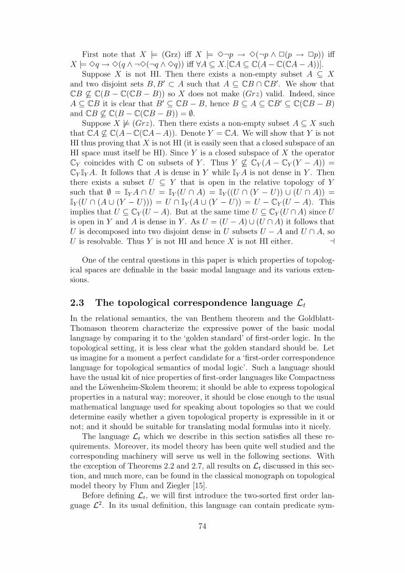
First note that X |= (Grz) iff X |= 3¬p → 3(¬p ∧ 2(p → 2p)) iffX |= 3q → 3(q ∧ ¬3(¬q ∧ 3q)) iff ∀A ⊆ X.[CA ⊆ C(A − C(CA − A))].

Suppose X is not HI. Then there exists a non-empty subset A ⊆ Xand two disjoint sets B,B′ ⊂ A such that A ⊆ CB ∩ CB′. We show thatCB 6⊆ C(B − C(CB − B)) so X does not make (Grz) valid. Indeed, sinceA ⊆ CB it is clear that B′ ⊆ CB − B, hence B ⊆ A ⊆ CB′ ⊆ C(CB − B)and CB 6⊆ C(B − C(CB − B)) = ∅.

Suppose X 6|= (Grz). Then there exists a non-empty subset A ⊆ X suchthat CA 6⊆ C(A−C(CA−A)). Denote Y = CA. We will show that Y is notHI thus proving that X is not HI (it is easily seen that a closed subspace of anHI space must itself be HI). Since Y is a closed subspace of X the operatorCY coincides with C on subsets of Y . Thus Y 6⊆ CY (A − CY (Y − A)) =CY IY A. It follows that A is dense in Y while IY A is not dense in Y . Thenthere exists a subset U ⊆ Y that is open in the relative topology of Ysuch that ∅ = IY A ∩ U = IY (U ∩ A) = IY ((U ∩ (Y − U)) ∪ (U ∩ A)) =IY (U ∩ (A ∪ (Y − U))) = U ∩ IY (A ∪ (Y − U)) = U − CY (U − A). Thisimplies that U ⊆ CY (U −A). But at the same time U ⊆ CY (U ∩A) since Uis open in Y and A is dense in Y . As U = (U −A) ∪ (U ∩A) it follows thatU is decomposed into two disjoint dense in U subsets U − A and U ∩ A, soU is resolvable. Thus Y is not HI and hence X is not HI either. ⊣

One of the central questions in this paper is which properties of topolog-ical spaces are definable in the basic modal language and its various exten-sions.

2.3 The topological correspondence language Lt

In the relational semantics, the van Benthem theorem and the Goldblatt-Thomason theorem characterize the expressive power of the basic modallanguage by comparing it to the ‘golden standard’ of first-order logic. In thetopological setting, it is less clear what the golden standard should be. Letus imagine for a moment a perfect candidate for a ‘first-order correspondencelanguage for topological semantics of modal logic’. Such a language shouldhave the usual kit of nice properties of first-order languages like Compactnessand the Lowenheim-Skolem theorem; it should be able to express topologicalproperties in a natural way; moreover, it should be close enough to the usualmathematical language used for speaking about topologies so that we coulddetermine easily whether a given topological property is expressible in it ornot; and it should be suitable for translating modal formulas into it nicely.

The language Lt which we describe in this section satisfies all these re-quirements. Moreover, its model theory has been quite well studied and thecorresponding machinery will serve us well in the following sections. Withthe exception of Theorems 2.2 and 2.7, all results on Lt discussed in this sec-tion, and much more, can be found in the classical monograph on topologicalmodel theory by Flum and Ziegler [15].

Before defining Lt, we will first introduce the two-sorted first order lan-guage L2. In its usual definition, this language can contain predicate sym-

74

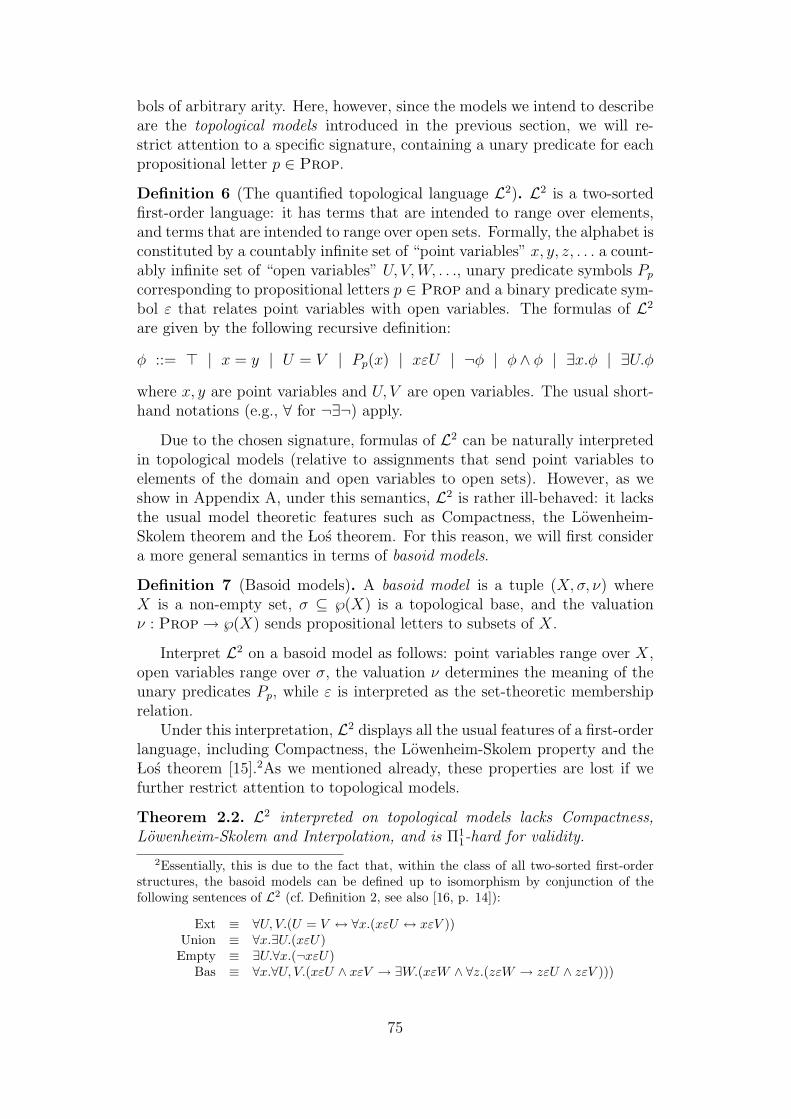
bols of arbitrary arity. Here, however, since the models we intend to describeare the topological models introduced in the previous section, we will re-strict attention to a specific signature, containing a unary predicate for eachpropositional letter p ∈ Prop.

Definition 6 (The quantified topological language L2). L2 is a two-sortedfirst-order language: it has terms that are intended to range over elements,and terms that are intended to range over open sets. Formally, the alphabet isconstituted by a countably infinite set of “point variables” x, y, z, . . . a count-ably infinite set of “open variables” U, V, W, . . ., unary predicate symbols Pp

corresponding to propositional letters p ∈ Prop and a binary predicate sym-bol ε that relates point variables with open variables. The formulas of L2

are given by the following recursive definition:

φ ::= ⊤ | x = y | U = V | Pp(x) | xεU | ¬φ | φ ∧ φ | ∃x.φ | ∃U.φ

where x, y are point variables and U, V are open variables. The usual short-hand notations (e.g., ∀ for ¬∃¬) apply.

Due to the chosen signature, formulas of L2 can be naturally interpretedin topological models (relative to assignments that send point variables toelements of the domain and open variables to open sets). However, as weshow in Appendix A, under this semantics, L2 is rather ill-behaved: it lacksthe usual model theoretic features such as Compactness, the Lowenheim-Skolem theorem and the ÃLos theorem. For this reason, we will first considera more general semantics in terms of basoid models.

Definition 7 (Basoid models). A basoid model is a tuple (X, σ, ν) whereX is a non-empty set, σ ⊆ ℘(X) is a topological base, and the valuationν : Prop → ℘(X) sends propositional letters to subsets of X.

Interpret L2 on a basoid model as follows: point variables range over X,open variables range over σ, the valuation ν determines the meaning of theunary predicates Pp, while ε is interpreted as the set-theoretic membershiprelation.

Under this interpretation, L2 displays all the usual features of a first-orderlanguage, including Compactness, the Lowenheim-Skolem property and theÃLos theorem [15].2As we mentioned already, these properties are lost if wefurther restrict attention to topological models.

Theorem 2.2. L2 interpreted on topological models lacks Compactness,Lowenheim-Skolem and Interpolation, and is Π1

1-hard for validity.

2Essentially, this is due to the fact that, within the class of all two-sorted first-orderstructures, the basoid models can be defined up to isomorphism by conjunction of thefollowing sentences of L2 (cf. Definition 2, see also [16, p. 14]):

Ext ≡ ∀U, V.(U = V ↔ ∀x.(xεU ↔ xεV ))Union ≡ ∀x.∃U.(xεU)Empty ≡ ∃U.∀x.(¬xεU)

Bas ≡ ∀x.∀U, V.(xεU ∧ xεV → ∃W.(xεW ∧ ∀z.(zεW → zεU ∧ zεV )))

75

The proof can be found in Appendix A.Thus, in order to work with topological models and keep the nice first-

order properties we need to somehow ‘tame’ L2. This is where Lt enters thepicture, a well behaved fragment of L2. Let us call an L2 formula α positive(negative) in an open variable U if all free occurrences of U are under aneven (odd) number of negation signs.

Definition 8 (The language Lt). Lt contains all atomic L2-formulas and isclosed under conjunction, negation, quantification over the point variablesand the following restricted form of quantification over open variables:

- if α is positive in the open variable U , and x is a point variable, then∀U.(xεU → α) is a formula of Lt,

- if α is negative in the open variable U , and x is a point variable, then∃U.(xεU ∧ α) is a formula of Lt.

(recall that φ → ψ is simply an abbreviation for ¬(φ ∧ ¬ψ)).

The reason Lt is particularly well-suited for describing topological modelslies in the following observation: Lt-formulas cannot distinguish between abasoid model and the topological model it generates. More precisely, for anybasoid model M = (X, σ, ν), let M = (X, σ, ν), where σ is the topologygenerated by the topological base σ.

Theorem 2.3 (Lt is the base-invariant fragment of L2). For any Lt-formula α(x1, . . . , xn, U1, . . . , Um), basoid model M = (X, σ, ν), and for alld1, . . . , dn ∈ X and O1, . . . , Om ∈ σ,

M |= α [d1, . . . , dn, O1, . . . , Om] iff M |= α [d1, . . . , dn, O1, . . . , Om] .

Moreover, every L2-formula φ(x1, . . . , xn, U1, . . . , Um) satisfying this invari-ance property is equivalent on topological models to an Lt-formula with thesame free variables.

It follows that Lt satisfies appropriate analogues of Compactness, theLowenheim-Skolem property, and the ÃLos theorem relative to the class oftopological models. Let us start with the Lowenheim-Skolem property. Calla topological model M = (X, τ, ν) countable if X is countable and τ has acountable base.

Theorem 2.4 (Lowenheim-Skolem for Lt). Let Γ be any set of Lt-formulas(in a countable signature). If Γ has an infinite topological model, then it hasa countable topological model.

Next, we will discuss an analogue of ÃLos’s theorem for Lt. First we needto define ultraproducts of topological models.

76

Definition 9 (Ultraproducts of basoid models). Let (Mi)i∈I be an indexedfamily of basoid models, where Mi = (Xi, σi, νi), and let D be an ultrafilterover the index set I. Define an equivalence relation ∼D on

∏i∈I Xi as follows:

x ∼D y iff {i | xi = yi} ∈ D

We define the ultraproduct∏

D Mi to be (X, σ, ν), where X = (∏

i∈I Xi)/∼D,

σ = {(∏

i∈I Oi)/∼D| each Oi ∈ σi}, and ν(p) = (

∏i∈I νi(p))/∼D

.If Mi = Mj for all i, j ∈ I, then

∏D Mi is called an ultrapower.

It is not hard to see that, under this definition, every ultraproduct of ba-soid models is again a basoid model. The same does not hold for topologicalmodels. Hence, rather than the basoid ultrapower

∏D Mi, we will use the

topological model it generates, i.e.,∏

D Mi. We will call the latter the topo-logical ultraproduct (or, topological ultrapower, if all factor models coincide).

Note that, by Theorem 2.3, the topological ultraproduct∏

D Mi cannot bedistinguished from the basoid ultraproduct

∏D Mi in Lt.

Theorem 2.5 (ÃLos theorem for Lt). Let α be any Lt-sentence, (Mi)i∈I anindexed set of topological models, and D an ultrafilter over I. Then

∏

D

Mi |= α iff {i ∈ I | Mi |= α} ∈ D

In particular, if N is a topological ultrapower of M, then for all Lt-formulasφ and assignments g, M |= φ [g] iff N |= φ [f · g], where f : M → N is thenatural diagonal embedding.

A typical use of ultraproducts is for proving compactness.

Theorem 2.6 (Compactness for Lt). Let Γ be any set of Lt-formulas. Ifevery finite subset of Γ is satisfiable in a topological model, then Γ itself issatisfiable in a topological ultraproduct of these models.

Another common use of ultraproducts is for obtaining saturated models.One can generalize this construction to topological models, provided thatthe notion of saturation is defined carefully enough. The following definitionof saturatedness is probably not the most general, but will suffice for thepurposes of this paper.

Definition 10 (Lt-saturatedness). By an Lt-type we will mean a set of Lt-formulas Γ(x) having exactly one free point variable x and no free openvariables. An open set O in a topological model is called point-saturated if,whenever all finite subtypes of an Lt-type Γ(x) are realized somewhere inO, then Γ(x) itself is realized somewhere in O. A topological model M =(X, τ, ν) is said to be Lt-saturated if the following conditions hold:

1. The entire space X is point-saturated.

77

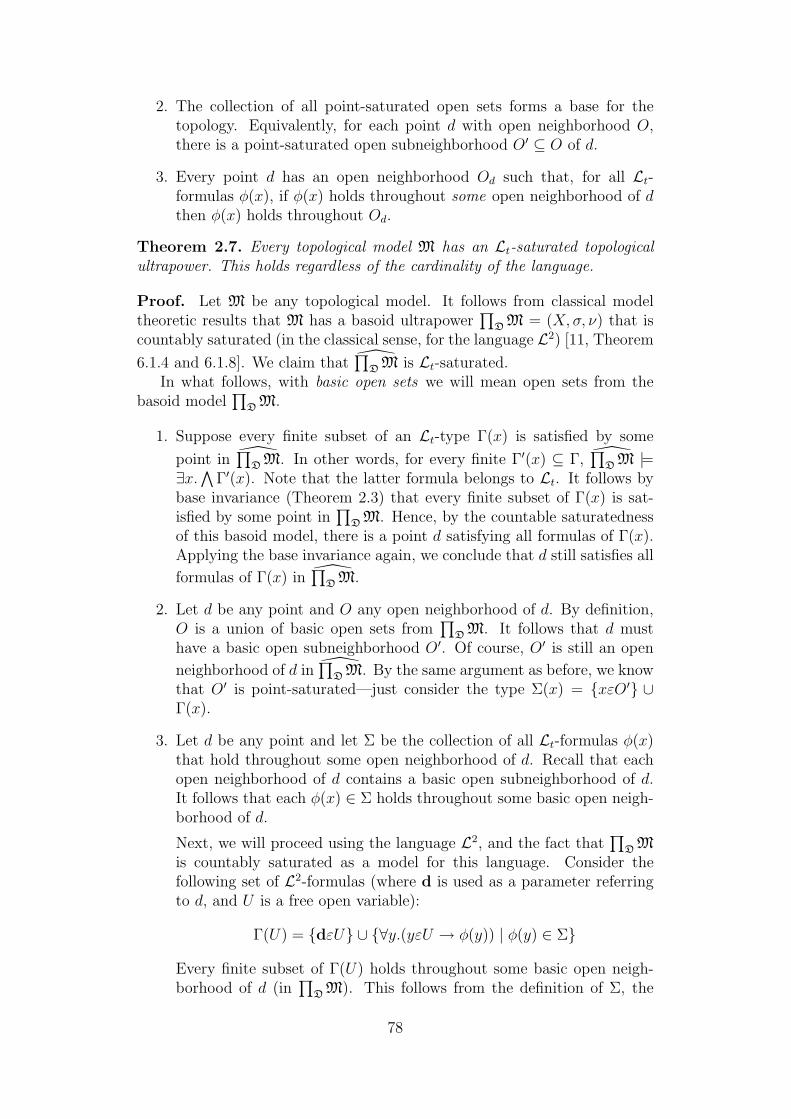
2. The collection of all point-saturated open sets forms a base for thetopology. Equivalently, for each point d with open neighborhood O,there is a point-saturated open subneighborhood O′ ⊆ O of d.

3. Every point d has an open neighborhood Od such that, for all Lt-formulas φ(x), if φ(x) holds throughout some open neighborhood of dthen φ(x) holds throughout Od.

Theorem 2.7. Every topological model M has an Lt-saturated topologicalultrapower. This holds regardless of the cardinality of the language.

Proof. Let M be any topological model. It follows from classical modeltheoretic results that M has a basoid ultrapower

∏D M = (X, σ, ν) that is

countably saturated (in the classical sense, for the language L2) [11, Theorem

6.1.4 and 6.1.8]. We claim that∏

D M is Lt-saturated.In what follows, with basic open sets we will mean open sets from the

basoid model∏

D M.

1. Suppose every finite subset of an Lt-type Γ(x) is satisfied by some

point in∏

D M. In other words, for every finite Γ′(x) ⊆ Γ,∏

D M |=∃x.

∧Γ′(x). Note that the latter formula belongs to Lt. It follows by

base invariance (Theorem 2.3) that every finite subset of Γ(x) is sat-isfied by some point in

∏D M. Hence, by the countable saturatedness

of this basoid model, there is a point d satisfying all formulas of Γ(x).Applying the base invariance again, we conclude that d still satisfies all

formulas of Γ(x) in∏

D M.

2. Let d be any point and O any open neighborhood of d. By definition,O is a union of basic open sets from

∏D M. It follows that d must

have a basic open subneighborhood O′. Of course, O′ is still an open

neighborhood of d in∏

D M. By the same argument as before, we knowthat O′ is point-saturated—just consider the type Σ(x) = {xεO′} ∪Γ(x).

3. Let d be any point and let Σ be the collection of all Lt-formulas φ(x)that hold throughout some open neighborhood of d. Recall that eachopen neighborhood of d contains a basic open subneighborhood of d.It follows that each φ(x) ∈ Σ holds throughout some basic open neigh-borhood of d.

Next, we will proceed using the language L2, and the fact that∏

D M

is countably saturated as a model for this language. Consider thefollowing set of L2-formulas (where d is used as a parameter referringto d, and U is a free open variable):

Γ(U) = {dεU} ∪ {∀y.(yεU → φ(y)) | φ(y) ∈ Σ}

Every finite subset of Γ(U) holds throughout some basic open neigh-borhood of d (in

∏D M). This follows from the definition of Σ, the

78

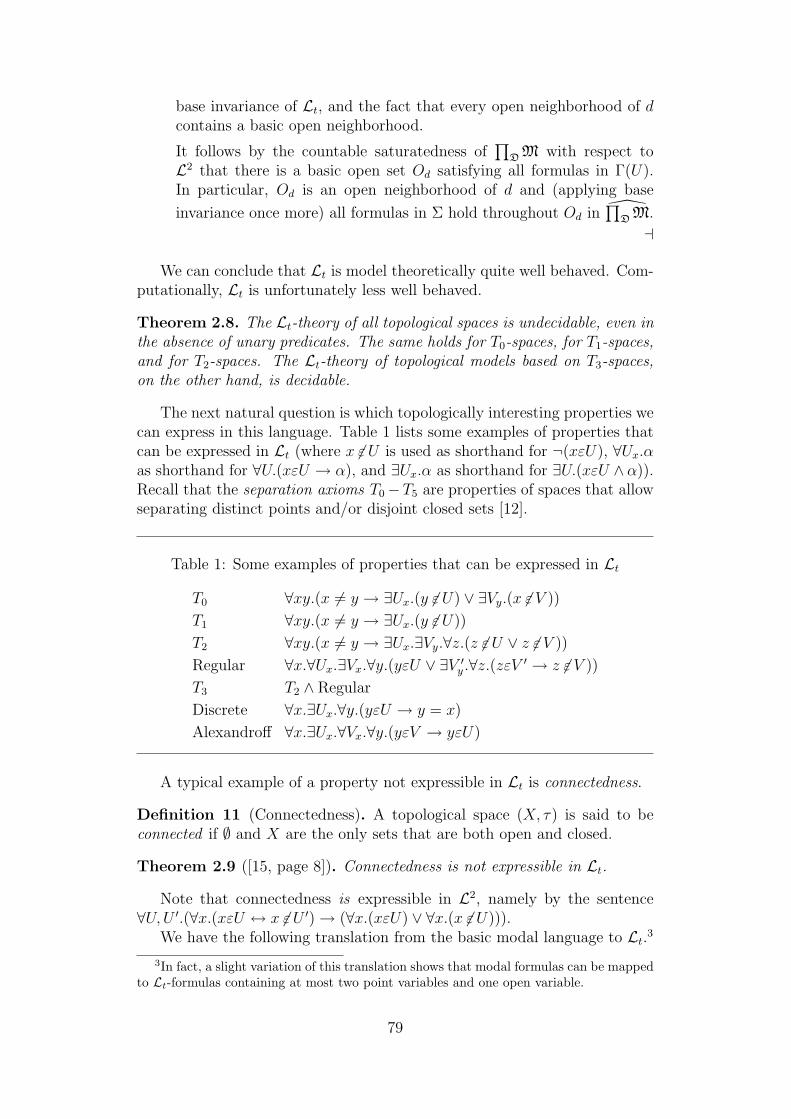
base invariance of Lt, and the fact that every open neighborhood of dcontains a basic open neighborhood.

It follows by the countable saturatedness of∏

D M with respect toL2 that there is a basic open set Od satisfying all formulas in Γ(U).In particular, Od is an open neighborhood of d and (applying base

invariance once more) all formulas in Σ hold throughout Od in∏

D M.

⊣

We can conclude that Lt is model theoretically quite well behaved. Com-putationally, Lt is unfortunately less well behaved.

Theorem 2.8. The Lt-theory of all topological spaces is undecidable, even inthe absence of unary predicates. The same holds for T0-spaces, for T1-spaces,and for T2-spaces. The Lt-theory of topological models based on T3-spaces,on the other hand, is decidable.

The next natural question is which topologically interesting properties wecan express in this language. Table 1 lists some examples of properties thatcan be expressed in Lt (where x 6εU is used as shorthand for ¬(xεU), ∀Ux.αas shorthand for ∀U.(xεU → α), and ∃Ux.α as shorthand for ∃U.(xεU ∧ α)).Recall that the separation axioms T0 −T5 are properties of spaces that allowseparating distinct points and/or disjoint closed sets [12].

Table 1: Some examples of properties that can be expressed in Lt

T0 ∀xy.(x 6= y → ∃Ux.(y 6εU) ∨ ∃Vy.(x 6ε V ))

T1 ∀xy.(x 6= y → ∃Ux.(y 6εU))

T2 ∀xy.(x 6= y → ∃Ux.∃Vy.∀z.(z 6εU ∨ z 6ε V ))

Regular ∀x.∀Ux.∃Vx.∀y.(yεU ∨ ∃V ′y .∀z.(zεV ′ → z 6ε V ))

T3 T2 ∧ Regular

Discrete ∀x.∃Ux.∀y.(yεU → y = x)

Alexandroff ∀x.∃Ux.∀Vx.∀y.(yεV → yεU)

A typical example of a property not expressible in Lt is connectedness.

Definition 11 (Connectedness). A topological space (X, τ) is said to beconnected if ∅ and X are the only sets that are both open and closed.

Theorem 2.9 ([15, page 8]). Connectedness is not expressible in Lt.

Note that connectedness is expressible in L2, namely by the sentence∀U,U ′.(∀x.(xεU ↔ x 6εU ′) → (∀x.(xεU) ∨ ∀x.(x 6εU))).

We have the following translation from the basic modal language to Lt.3

3In fact, a slight variation of this translation shows that modal formulas can be mappedto Lt-formulas containing at most two point variables and one open variable.

79

Definition 12. [Standard translation] The standard translation ST from thebasic modal language ML into Lt is defined inductively:

STx(⊤) = ⊤STx(p) = Pp(x)STx(¬φ) = ¬STx(φ)STx(φ ∧ ψ) = STx(φ) ∧ STx(ψ)STx(2φ) = ∃U.(xεU ∧ ∀y.(yεU → STy(φ)))

where x, y are distinct point variables and U is an open variable.

Theorem 2.10. For M a topological model and ϕ ∈ ML a modal formula,M, a |= ϕ iff M |= STx(ϕ)[a]

Proof. By induction on the complexity of ϕ. ⊣

In other words, modal formulas can be seen as Lt-formulas in one freevariable, and sets of modal formulas can be seen as Lt-types in the senseof Definition 10. This shows that all the above results on Lt also apply tomodal formulas. For example,

Theorem 2.11 (Lowenheim-Skolem theorem for ML). Let Σ ⊆ ML bea set of modal formulas (in a countable signature). If Σ is satisfied in atopological model, then it is satisfied in a countable topological model.

80

The expressive power of the basic modal language on relational structuresis relatively well understood. The Van Benthem theorem characterizes themodally definable properties of points in Kripke models, in terms of bisim-ulations, while the Goldblatt-Thomason theorem characterizes modal defin-ability of classes of Kripke frames, in terms of closure under operations suchas disjoint union.

In this section, we will prove topological analogs of these results. First,we present a topological version of Van Benthem’s theorem, using the notionof topo-bisimulations [1]. Next, we identify four operations on topologicalspaces that preserve validity of modal formulas. Finally, we apply these clo-sure conditions in order to determine which Lt-definable classes are modallydefinable, and vice versa.

3.1 Topological bisimulations

In this section we characterize the modal fragment of Lt in terms of topo-bisimulations.

Definition 13. Consider topological models M = (X, ν) and M′ = (X ′, ν ′).A non-empty relation Z ⊆ X ×X ′ is a topo-bisimulation between M and M′

if the following conditions are met for all x ∈ X and x′ ∈ X ′:

Zig If xZx′ and x ∈ O ∈ τ then there exists O′ ∈ τ ′ such that x′ ∈ O′ andfor all y′ ∈ O′ there exists a y ∈ O such that yZy′.

Zag If xZx′ and x′ ∈ O′ ∈ τ ′ then there exists O ∈ τ such that x ∈ O andfor all y ∈ O there is a y′ ∈ O′ such that yZy′.

Atom If xZx′ then x ∈ ν(p) iff x′ ∈ ν ′(p) for all p ∈ Prop.

Elements x ∈ X and x′ ∈ X ′ are said to be bisimilar, denoted by(M, x)↔(M′, x′), if there exists a bisimulation Z between M and M′ suchthat xZx′.

This definition can be formulated more naturally if we use some standardmathematical notation. For a binary relation Z ⊆ X ×X ′ and a set A ⊆ X,let us denote by Z[A] the image {x′ ∈ X ′ | ∃x ∈ A.(xZx′)}, and let us definethe preimage Z−1[A′] of a set A′ ⊆ X ′ analogously.

Proposition 3.1. The Zig and Zag conditions in Definition 13 are equiv-alent to the following:

Zig′ For all O ∈ τ , Z[O] ∈ τ ′.

81

Chapter 3

First Steps

Zag′ For all O′ ∈ τ , Z−1[O′] ∈ τ .

Proof. We will only show the equivalence for Zig′, the proof for Zag′ isanalogous. In one direction, suppose that Z satisfies Zig, and take an openO ∈ τ . The Zig condition ensures that, for each x′ ∈ Z[O], we can find anopen neighborhood O′ ∈ τ ′ with x′ ∈ O′, such that O′ ⊆ Z[O]. It followsthat Z[O], being the union of these neighborhoods, is open in τ ′. For theother direction, suppose Z[O] ∈ τ ′ holds for all O ∈ τ . Consider an arbitraryx ∈ O ∈ τ and x′ ∈ X ′ such that xZx′. Then Z[O] qualifies for an openneighborhood O′ of x′ satisfying the condition Zig since x′ ∈ Z[O] ∈ τ ′. ⊣

In what follows, we will freely use this equivalent formulation whenever itis convenient. Topo-bisimulations are closely linked with the notion of modalequivalence.

Definition 14. We say that two pointed topological models (M, x) and(M′, x′) are modally equivalent and write (M, x) ! (M′, x′) if for all formulasφ ∈ ML, (M, x) |= φ iff (M′, x′) |= φ.

Theorem 3.2 ([1]). For arbitrary topological pointed models (M, x) and(M′, x′), if (M, x)↔(M′, x′) then (M, x) ! (M′, x′).

Proof. The proof proceeds via straightforward induction on the complexityof modal formulas. We only treat the case φ = 2ψ.

Suppose (M, x) |= 2ψ. Then there exists an open neighborhood O of xsuch that O |= ψ. By Zig we obtain that Z[O] is an open neighborhood ofx′ and, by induction hypothesis, Z[O] |= ψ. Therefore (M′, x′) |= 2ψ. Theother direction is proved similarly. ⊣

The converse does not hold in general, but it holds on a restricted classof Lt-saturated topological models.

Theorem 3.3. Let M and M′ be Lt-saturated topological models, and sup-pose that (M, x) ! (M′, x′). Then (M, x)↔(M′, x′).

Proof. Let M = (X, τ, ν) and M′ = (X ′, τ ′, ν ′), and let Z ⊆ X ×X ′ be themodal indistinguishability relation (i.e., xZx′ iff (M, x) ! (M′, x′)). Wewill show that Z is a topo-bisimulation, and hence, (M, x)↔(M′, x′). Thatthe Atom condition holds follows immediately from the construction of Z.In the remainder of this proof, we will show that Zag holds. The case forZig is analogous.

Consider any a, a′ such that aZa′, and let O′ ∈ τ ′ be an open neigh-borhood of a′. Since M′ is Lt-saturated, we may assume that O′ is point-saturated (if not, just take a point-saturated subneighborhood of a′). Weneed to find an open neighborhood O of a such that for each b ∈ O thereexists a b′ ∈ O′ with bZb′.

By Lt-saturatedness of M, we know that a has an open neighborhood Oa

such that, for every modal formula φ, if a |= 2φ then φ holds throughoutOa. Dually, this means that

82

(*) For any b ∈ Oa and modal formula φ, if b |= φ then a |= 3φ.

To show that Oa meets the requirements of the Zag condition, considerany b ∈ Oa. We will find a b′ ∈ O′ such that bZb′. Let Σb be the set ofmodal formulas true at b. Every finite subset of Σb is satisfied somewherein O′. For, consider any finite Σ′ ⊆ Σb. Then by (*), M, a |= 3

∧Σ′, and

hence M′, a′ |= 3∧

Σ′. Therefore∧

Σ′ must be satisfied somewhere in O′.Recall that O′ is point-saturated. We conclude that there is a point b′ ∈ O′

satisfying Σb. It follows that (M, b) ! (M′, b′), and hence bZb′. ⊣

Combining this with Theorem 2.7, we obtain

Theorem 3.4. An Lt-formula α(x) is invariant under topo-bisimulations iffit is equivalent to the standard translation of a modal formula.

Proof. Easily adapted from the proof of the van Benthem CharacterizationTheorem for relational semantics (see e.g. [8, Theorem 2.68] for details). ⊣

3.2 Alexandroff extensions

We saw in Part II (section 2.1) the three validity-preserving operations ontopological spaces — taking open subspaces, topological sums and interiorimages. We also introduced a new construction of Alexandroff extensionsthat anti-prserves validity. Here we recall this definition identify a connectionbetween Alexandroff extensions and topological ultraproducts.

Definition 15 (Alexandroff extensions). A filter F ⊆ ℘(X) over a topologi-cal space (X, τ) is called open if for all A ∈ F , also IA ∈ F . The Alexandroffextension of a space (X, τ) is the space X∗ = (UfX, τ ∗), where UfX is theset of ultrafilters over X, and τ ∗ is the topology over UfX generated by thesets of the form {u ∈ UfX | F ⊆ u} for F an open filter over X.

Theorem 3.5. For any space X, X∗ is Alexandroff.

Proof. For any point u ∈ X∗ consider a filter F generated by all opensets that belong to u. Then the set {v ∈ X∗ | F ⊆ v} is a least openneighborhood of u. It follows that v is in the least open neighborhood of u

iff for each IA ∈ u we have IA ∈ v iff CA ∈ u for each A ∈ v. ⊣

Note that the map π : X → X∗ that sends a ∈ X to the correspondingprincipal ultrafilter πa need not be open, or even continuous [7, Example5.13]. Indeed the image π(X), as a subspace of X∗, might not be homeomor-phic to X—as soon as X is T1 the subspace π(X) is discrete. Nevertheless,it is worth mentioning that the topology τ ∗ preserves the information aboutthe original topology τ in a curious way. It is an easy exercise for the readerfamiliar with ultrafilter convergence (see, e.g., [12, pp. 91-93]) that u ∈ X∗

belongs to the least open neighborhood of the principal ultrafilter πa in X∗

iff u → a (i.e. u converges to a ∈ X according to τ).Basic open sets of the Alexandroff extension X∗ have a nice character-

isation that follows immediately from their definition. For any topologicalspace X and subset A ⊆ X, let A∗ = {u ∈ X∗ | A ∈ u}. It easily seen that:

83

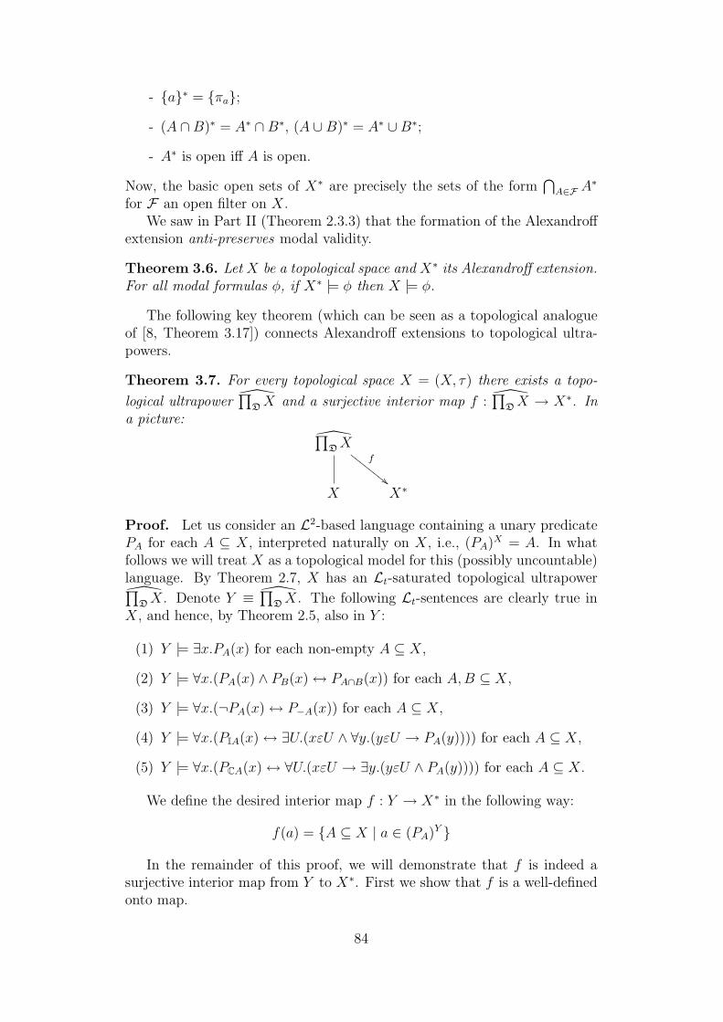
- {a}∗ = {πa};

- (A ∩ B)∗ = A∗ ∩ B∗, (A ∪ B)∗ = A∗ ∪ B∗;

- A∗ is open iff A is open.

Now, the basic open sets of X∗ are precisely the sets of the form⋂

A∈F A∗

for F an open filter on X.We saw in Part II (Theorem 2.3.3) that the formation of the Alexandroff

extension anti-preserves modal validity.

Theorem 3.6. Let X be a topological space and X∗ its Alexandroff extension.For all modal formulas φ, if X∗ |= φ then X |= φ.

The following key theorem (which can be seen as a topological analogueof [8, Theorem 3.17]) connects Alexandroff extensions to topological ultra-powers.

Theorem 3.7. For every topological space X = (X, τ) there exists a topo-

logical ultrapower∏

D X and a surjective interior map f :∏

D X → X∗. Ina picture:

∏D X

f

""F

F

F

F

F

F

F

F

X X∗

Proof. Let us consider an L2-based language containing a unary predicatePA for each A ⊆ X, interpreted naturally on X, i.e., (PA)X = A. In whatfollows we will treat X as a topological model for this (possibly uncountable)language. By Theorem 2.7, X has an Lt-saturated topological ultrapower∏

D X. Denote Y ≡∏

D X. The following Lt-sentences are clearly true inX, and hence, by Theorem 2.5, also in Y :

(1) Y |= ∃x.PA(x) for each non-empty A ⊆ X,

(2) Y |= ∀x.(PA(x) ∧ PB(x) ↔ PA∩B(x)) for each A,B ⊆ X,

(3) Y |= ∀x.(¬PA(x) ↔ P−A(x)) for each A ⊆ X,

(4) Y |= ∀x.(PIA(x) ↔ ∃U.(xεU ∧ ∀y.(yεU → PA(y)))) for each A ⊆ X,

(5) Y |= ∀x.(PCA(x) ↔ ∀U.(xεU → ∃y.(yεU ∧ PA(y)))) for each A ⊆ X.

We define the desired interior map f : Y → X∗ in the following way:

f(a) = {A ⊆ X | a ∈ (PA)Y }

In the remainder of this proof, we will demonstrate that f is indeed asurjective interior map from Y to X∗. First we show that f is a well-definedonto map.

84

• For any a ∈ Y , f(a) is an ultrafilter over X.

Recall that an ultrafilter over X is any set u of subsets of X satisfying(i) A∩B ∈ u iff both A ∈ u and B ∈ u, and (ii) A ∈ u iff (X \A) 6∈ u.By (2) and (3) above, f(a) indeed satisfies these properties.

• f is surjective (i.e., every ultrafilter over X is f(a) for some a ∈ Y ).

Take u ∈ X∗, and let Γu(x) = {PA(x) | A ∈ u}. It follows from (1)and (2) that every finite subset of Γu(x) is satisfied by some point in Y .Since Y is point-saturated, there exists a ∈ Y satisfying Γu(x), hencef(a) = u.

Next we show that f is open and continuous. Note that by Proposition 3.1it suffices to prove that the graph of f is a topo-bisimulation.

Take arbitrary a ∈ Y and let Oa be as described in Definition 10. LetOu be a least open neighborhood of u = f(a). We proceed by verifying theconditions Zig and Zag for the pair (a, u).

• Zig. Take arbitrary O′ such that a ∈ O′. By Lt-saturatedness of Y ,there exists a point-saturated O ⊆ O′ such that a ∈ O.

Take arbitrary v ∈ Ou. We will find a b ∈ O such that v = f(b). Let

Γv(x) = {PA(x) | A ∈ v}

Every finite subset of Γv(x) is satisfied somewhere in O. Indeed, ifPA1

, . . . , PAn∈ Γv, denote B ≡

⋂i Ai. Then B ∈ v and hence CB ∈ u.

Therefore Y |= PCB(a). It follows by (5) that PB holds somewhere inO. By the point-saturatedness of O we may conclude that some b ∈ Osatisfies all of Γv(x), and hence f(b) = v.

• Zag. It suffices to show that for any b ∈ Oa we have f(b) ∈ Ou.Suppose the contrary. Then we have b ∈ Oa and f(b) 6∈ Ou. The lattermeans that there exists a set A ⊆ X such that A ∈ f(b) but CA 6∈ u.From A ∈ f(b) we obtain Y |= PA(b). While CA 6∈ u iff −CA ∈ u

iff I−A ∈ u iff Y |= PI−A(a) iff Y |= ∃U.[aεU ∧∀y.(yεU → P−A(y))]iff P−A(x) is true throughout some open neighborhood of a iff P−A(x)is true throughout Oa, which contradicts Y |= PA(b) since b ∈ Oa.

⊣

3.3 Modal definability vs Lt-definability

In this section we are seeking necessary and sufficient conditions, in the spiritof the Goldblatt-Thomason theorem, for a class of topological spaces to bemodally definable. We have already found some necessary conditions: wehave seen that every modally definable class of topological spaces is closedunder the formation of topological sums, open subspaces and interior imagesand reflects Alexandroff extensions. Our aim is to prove a converse, in otherwords, to characterize modal definability in terms of these closure properties.

85

Theorem 3.8. Let K be any Lt-definable class of topological spaces. ThenK is modally definable iff it is closed under taking open subspaces, interiorimages, topological sums and it reflects Alexandroff extensions.

Proof. We will only prove the difficult right-to-left direction. The left-to-right direction already follows from theorems 2.1.2, 2.1.5 and 2.1.8 of Part IIand Theorem 3.6.

Let K be any class satisfying the given closure conditions. Take the setLog(K) of modal formulas valid on K. We will show that, whenever X |=Log(K), then X ∈ K. In other words, Log(K) defines K.

Suppose X |= Log(K) for some topological space X. Introduce a propo-sitional letter pA for each subset A ⊆ X, and let ν be the natural valuationon X for this (possibly uncountable) language, i.e. ν(pA) = A for all A ⊆ X.Let ∆ be the set of all modal formulas of the following forms (where A,Brange over subsets of X):

pA∩B ↔ pA ∧ pB

p−A ↔ ¬pA

pIA ↔ 2pA

pCA ↔ 3pA

By definition, ∆ is valid on M = (X, ν). Note that the standard translationsof the formulas in ∆ correspond exactly to the formulas listed in conditions(2)–(5) of Theorem 3.7 (in the corresponding Lt-language, which has a one-place predicate PA(x) for each A ⊆ X). What is missing is the condition (1).The following claim addresses this.

Claim: For each a ∈ X there is a model Na = (Ya, µa) withYa ∈ K, such that Na |= ∆ and some point in Na satisfies pa.

Proof. Take any a ∈ X, and let ∆a = {2ϕ | ϕ ∈ ∆} ∪{p{a}

}.

As a first step, we will show that there is a topological model K

based on a space in K, such that some point a′ of K satisfies ∆a.By the compactness of Lt (Theorem 2.6), it suffices to show thatevery finite conjunction δ of formulas in ∆a is satisfiable on K.Since δ is satisfied at a in M and M |= Log(K), ¬δ cannot belongto Log(K). Hence δ is satisfiable on K.

By Theorem 2.7 we may assume K is Lt-saturated. Let Oa′ bean open neighborhood of a′ as described in Definition 10, and letNa be the submodel of K based on Oa′ . Then Na satisfies allrequirements of the claim. ⊣

Note how, in the above argument, we used the fact that K is Lt-definable(for the compactness argument, and for the saturation), and that it is closedunder taking open subspaces. Next, we will use the fact that K is closedunder taking topological sums.

86

Let Y =⊎

a∈X Ya, and let N = (Y, µ), where µ is obtained from theµa’s in the obvious way. By closure under taking topological sums, Y ∈ K.Moreover, by Theorem 2.1.2 of Part II, N |= ∆. Finally, each pA, for non-empty A ⊆ X, holds at some point in N (more precisely, at some pointin Na for any a ∈ A). It follows (using the standard translation) that theconditions (1)–(5) from the proof of Theorem 3.7 hold for N.

We can now proceed as in the proof of Theorem 3.7, and construct aninterior map from an ultrapower of N onto the Alexandroff extension X∗

of X. Since K is closed under topological ultrapowers (Theorem 2.5) andimages of interior maps, and reflecs Alexandroff extensions, we conclude thatX ∈ K. ⊣

Inspection of the proof shows that Theorem 3.8 applies not only to Lt-definable classes but to any class of spaces closed under ultraproducts. Infact, by Lemma 3.9 below, closure under ultrapowers suffices. Some fur-ther improvements are still possible. Most importantly, using algebraic tech-niques, we will show in the next section that closure under Alexandroff ex-tensions already suffices. For the complete picture, see Corollary 3.15.

The opposite question. Theorem 3.8 characterizes, among all Lt-definable classes of topological spaces, those that are modally definable. Itmakes sense to ask the opposite question: which modally definable classes ofspaces are Lt-definable? In classical modal logic the answer was provided byvan Benthem in [3] (see also [19]). We follow the route paved in these papers.First we prove a topological analogue of an observation due to Goldblatt:

Lemma 3.9. An ultraproduct of topological spaces is homeomorphic to anopen subspace of the ultrapower (over the same ultrafilter) of their topologicalsum.

Proof. Suppose (Xi)i∈I is a family of topological spaces and D is an ul-trafilter over I. Denote by X =

⊎i∈I Xi the topological sum of Xi and by

Y =∏

D Xi their topological ultraproduct. Take arbitrary a : I →⊎

i∈I Xi

such that a(i) ∈ Xi. Then a can be viewed both as an element of∏

i∈I Xi and

as an element of∏

i∈I X. This defines a natural embedding from Y into∏

D Xwhich is clearly injective. That this embedding is open is easily seen (recallthat this suffices to be checked on the elements of the base). To show that itis also continuous, suppose [a]D ∈

∏D X is such that A = {i | a(i) ∈ Xi} ∈ D

(so [a]D comes from Y ). Then any basic ultrabox neighborhood∏

D Oi of[a]D is such that B = {i | a(i) ∈ Oi ⊆ X} ∈ D. We clearly have A ∩ B ∈ D,so

∏D(Oi ∩ Xi) is another open neighborhood of [a]D, now also in Y . The

required continuity follows. Since we have established that Y can be embed-

ded into∏

D X by an interior map, it follows that Y is homeomorphic to an

open subspace of∏

D X. ⊣

We are one step away from finding a nice criterion for a modally defin-able class to be Lt-definable. It follows from Garavaglia’s theorem [16] (the

87

topological analogue of the Keisler-Shelah Theorem) that a class K of spacesis Lt-definable iff K is closed under isomorphisms and ultraproducts and thecomplement of K is closed under ultrapowers.

Theorem 3.10. A modally definable class K of spaces is Lt-definable iff itis closed under ultrapowers.

Proof. If K is Lt-definable, then it is clearly closed under ultrapowers. Forthe converse direction take a modally definable class K that is closed underultrapowers. Then K is closed under topological sums and open subspaces.It follows from Lemma 3.9 that K is closed under ultraproducts. It is easilyseen that any modally definable class is closed under Lt-isomorphisms. Itfollows from Theorems 2.5 and 2.10 that the complement of K is closed underultrapowers. Hence K is Lt-definable. ⊣

Since modally definable classes are closed under interior images and ultra-powers are interior images of box products via the canonical quotient map,we obtain

Corollary 3.11. A modally definable class of spaces that is closed under boxpowers is Lt-definable.

Separating examples. To close this section we give examples separat-ing Lt-definability from modal definability. We have exhibited earlier Lt-sentences defining the separation axioms T0 − T2. We have also shown inTheorem 2.1.9 of Part II that T0 − T2 are not definable in the basic modallanguage. Thus we have examples of Lt-definable classes of spaces that arenot modally definable.

To show that there are modally definable classes of spaces that are notLt-definable requires more work. Recall that the class of Hereditarily Irre-solvable (HI) spaces is modally definable (Theorem 2.1). This class is notLt-definable. We will use the following lemma:

Lemma 3.12. Any class K of spaces that is both modally definable and Lt-definable is closed under Alexandroff extensions.

Proof. Suppose X ∈ K. By Theorem 3.7 there exists a topological ultra-power Y of X and an onto interior map f : Y → X∗. Being an Lt-definableclass, K is closed under topological ultrapowers. Hence Y ∈ K. Being amodally definable class, K is closed under interior images. Therefore X∗ ∈ K,as required. ⊣

Theorem 3.13. The class of HI spaces is not Lt-definable.

Proof. By Theorem 2.1 and the above lemma, to prove that the class of HIspaces is not Lt-definable it suffices to show that this class is not closed underAlexandroff extensions. In [7, Example 5.12] a space X is exhibited that isHI, but its Alexandroff extension is not HI. We reproduce this example forreader’s convenience.

88

Let X = (N, τ) be a topological space with carrier N = {1, 2, . . . } andtopology τ = {[1, n) | n ∈ N} ∪ N. This is the Alexandroff topology corre-sponding to the order ≥. To show that X is HI, observe first that for anarbitrary subset A ⊆ N we have CA = [min A,∞). Further, if A,A′ ⊆ Bare such that A ∩ A′ = ∅ it is easily seen that either min A > min B ormin A′ > min B. Hence either B 6⊆ CA or B 6⊆ CA′. This shows that nosubset of X can be decomposed into two disjoint dense in it sets, so X is HI.

Consider the Alexandroff extension X∗. Let F ⊆ X∗ denote the set of allthe free ultrafilters over X. Fix two distinct free ultrafilters u, v ∈ F. Wewill show that both u and v belong to the least open neighborhood of anyw ∈ F. To see this it suffices to check that for any non-empty A ⊆ X wehave CA ∈ w. But if A is non-empty, then CA = [min A,∞) is cofinite andthus belongs to the free ultrafilter w. It follows that {u} and {v} are twodisjoint dense in F subsets. Hence X∗ is not HI. ⊣

3.4 Interlude: an algebraic perspective

In Part II (Theorem 2.3.4) we have proved the following theorem using alge-braic techniques and duality theory:

Theorem 3.14. The class K of topological spaces which is closed under theformation of Alexandroff extensions is modally definable iff it is closed un-der taking open subspaces, interior images, topological sums and it reflectsAlexandroff extensions.

Another characterization of the modal definability for topological spacesthat applies to any class of spaces is contained in [7, Theorem 5.10] andis also based on the duality outlined in this section. For the co-algebraicperspective on modal definability that encompasses both the relational andthe topological cases, as well as more general semantical frameworks, we referto [24].

Combining Theorem 3.14 with Theorem 3.7, we obtain our most generalversion of the definability theorem for the basic modal language:

Corollary 3.15. Let K be a class of topological spaces satisfying at least oneof the following conditions:

(i) K is Lt-definable;

(ii) K is closed under box powers;

(iii) K is closed under ultrapowers;

(iv) K is closed under Alexandroff extensions.

then K is modally definable iff it is closed under taking open subspaces, inte-rior images, topological sums and it reflects Alexandroff extensions.

89

Proof. The easier ‘only if’ part follows from theorems 2.1.2, 2.1.5 and 2.1.8of Part II and theorem 3.6.

To prove the ‘if’ part suppose that K is closed under taking open sub-spaces, interior images, topological sums and it reflects Alexandroff exten-sions. Let us prove that under these conditions, if K satisfies any of theconditions (i)-(iii) above, then it also satisfies the condition (iv).

First we show that each of (i) and (ii) implies (iii). Indeed, if K is Lt-definable, then it is closed under ultrapowers; also, if K is closed under boxpowers, since ultrapowers are interior images of box powers under the canon-ical quotient map and K is closed under interior images, we obtain that K isclosed under ultrapowers.

Next we show that (iii) implies (iv). Indeed, it follows from Theorem 3.7and the closure under interior images that if K is closed under taking ultra-powers, then K is closed under Alexandroff extensions.

Thus, in any of the cases (i)-(iv), K is closed under Alexandroff extensions.Now apply Theorem 3.14. ⊣

The analogue of Theorem 3.7 for relational semantics has a neat algebraicproof [18]. A similar proof for the topological case is lacking and we leavethis as a challenge for the interested reader.

90

In order to increase the topological expressive power of the basic modallanguage, various extensions have been proposed. For instance, Shehtman[28] showed that connectedness becomes definable when the basic modal lan-guage is enriched with the global modality. Similarly, T0, T1 and density-in-itself become definable when we enrich the basic modal language either withnominals or with the difference modality. In this section, we show exactlyhow much definable power we gain by these additions, by giving analoguesof Theorem 3.8 for these extended languages. Our findings are summarizedin Table 2 and 3 on page 102 and 103.

We believe Theorem 3.4 could also be generalized to the languages studiedin this section, using appropriate analogues of topo-bisimulations. However,we have decided not to pursue this here suspecting the lack of many newinsights.

4.1 The global modality

In the basic modal language with 3 and 2, one can only make statementsabout points that are arbitrarily close to the current point of evaluation. Itappears impossible to say, for instance, that there is a point satisfying p (i.e.,to express non-emptyness of p). The global modality, denoted by E, givesus the ability to make such global statements. For example, Ep expressesnon-emptyness of the set p, and A(p → q) expresses that p is contained in q.

Formally, M(E) extends the basic modal language with an extra operatorE that has the following semantics:

M, w |= Eφ iff ∃v ∈ X. (M, v |= φ)

The dual of E is denoted by A, i.e., Aϕ is short for ¬E¬ϕ. The standardtranslation can be extended in a straightforward way, by letting STx(Eφ) =∃x.(STx(φ)). In other words, M(E) is still a fragment of Lt.

Shehtman [28] showed that connectedness can be defined using the globalmodality:

Proposition 4.1. A(2p ∨ 2¬p) → Ap ∨ A¬p defines connectedness.

As connectedness is not definable in the basic modal language (Theorem2.1.4 of Part II), this shows that M(E) is more expressive than the basicmodal language. As a consequence of this increased expressive power, certainoperations on spaces do not preserve validity anymore.

Proposition 4.2. Taking open subspaces, or taking topological sums, in gen-eral does not preserve validity of M(E)-formulas.

91

Chapter 4

Extended Modal Languages

Proof. It suffices to show that connectedness is not preserved by these twooperations. The real interval (0, 1), with the usual topology, is connected,but its open subspace (0, 1

2)∪ (1

2, 1) is not. Likewise, for any connected space

X, the topological sum X⊎

X is no longer connected. ⊣

Taking interior images, on the other hand, does preserve validity ofM(E)-formulas, and taking Alexandroff extensions anti-preserves it. In fact,these two operations characterize definability in M(E), as the following ana-logue of Theorem 3.8 shows.

Theorem 4.3. Let K be any Lt-definable class of topological spaces. ThenK is definable in the basic modal language with global modality iff it is closedunder interior images and it reflects Alexandroff extensions.

Proof. The ‘only if’ direction is a straightforward adaptation of Theorem2.1.8 of Part II and Theorem 3.6. The proof of the ‘if’ direction is essentiallya simplification of the proof of Theorem 3.8: suppose X is a topological spacevalidating the M(E)-theory of K, and let ∆ be the following set of formulas,for all B, C ⊆ X:

EpB for non-empty BA(pB∩C ↔ pB ∧ pC)A(p−B ↔ ¬pB)A(pIB ↔ 2pB)A(pCB ↔ 3pB)

Note that these formulas exactly correspond to conditions (1)–(5) from theproof of Theorem 3.7. As in the proof of Theorem 3.8, we can find a topo-logical model N = (Y, µ) with Y ∈ K, such that N |= ∆. Finally, we proceedas in the proof of Theorem 3.7, and construct an interior map from an ul-trapower of N onto the Alexandroff extension X∗ of X. Since K is closedunder topological ultrapowers (Theorem 2.5) and images of interior maps,and reflects Alexandroff extensions, we conclude that X ∈ K. ⊣

4.2 Nominals

Another natural extension of the basic modal language is with nominals.Nominals are propositional variables that denote singleton sets, i.e., theyname points. In point-set topology one often finds definitions that involveboth open sets and individual points. In the language Lt, one can refer to thepoints in the space by means of point variables. The basic modal languagelacks such means, and nominals can be seen as a way to solve this problem.Here are some examples of properties that can be defined using nominals:

T0 @i3j ∧ @j3i → @ijT1 3i → iDensity-in-itself 3¬i

92

These properties are not definable in the basic modal language (Theorem2.1.9 of Part II). T2-separation, on the other hand, remains undefinable evenwith nominals (Theorem 4.9).

Modal languages containing nominals are often called hybrid languages.In this section we investigate the topological expressive power of two hybridlanguages, namely H(@) and H(E). Formally, fix a countably infinite setof nominals Nom = {i1, i2, . . .}, disjoint from the set Prop of propositionletters. Then the formulas of H(@) are given by the following recursivedefinition:

H(@) φ ::= ⊤ | p | i | φ ∧ φ | ¬φ | 2φ | @iφ

where p ∈ Prop and i ∈ Nom. H(E) further extends H(@) with the globalmodality, which was described in the previous section. Thus, the formulasof H(E) are given by the following recursive definition:

H(E) φ ::= ⊤ | p | i | φ ∧ φ | ¬φ | 2φ | @iφ | Eφ

As in the previous section, we will use Aφ as an abbreviation for ¬E¬φ. Wehave introduced @i as a primitive operator, but it will become clear afterintroducing the semantics that @i can be defined in terms of the operator E.

Definition 16. A hybrid topological model M is a topological space (X, τ)and a valuation ν : Prop ∪ Nom → ℘(X) which sends propositional lettersto subsets of X and nominals to singleton sets of X.

The semantics for H(@) and H(E) is the same as for the basic modallanguage for the propositional letters, nominals, Boolean connectives, andthe modality 2. The semantics of @ and E is as follows:

M, w |= @iφ iff M, v |= φ for ν(i) = {v}M, w |= Eφ iff ∃v ∈ X.(M, v |= φ)

Validity and definability are defined as for the basic modal language, butconsidering only valuations that assign singleton sets to the nominals.

Proposition 4.4. Taking topological sums or interior images in general doesnot preserve validity of H(@)-formulas.

Proof. The one-point space X = {0} with the trivial topology validates@i3j, but this formula is not valid on X

⊎X. Thus topological sums do not

preserve validity for H(@).To see that H(@)-validity is not preserved by interior maps, consider

natural numbers with the topology induced by the ordering, i.e. the space(N, τ) where τ = {[a,∞) | a ∈ N} ∪ {∅}. The formula ϕ = @i2(3i → i)(which defines antisymmetry in the relational case) is easily seen to be validin it. Then consider a topological space X = {0, 1} with the trivial topologyτ ′ = {∅, X} and a map f that sends even numbers to 0 and odd numbers to1. This is an interior map, however, ϕ is not even satisfiable on X. ⊣

93

On the other hand, the validity of H(@)-formulas is preserved undertaking open subspaces.

Lemma 4.5. The validity of H(@) formulas is preserved under taking opensubspaces.

The proof is identical to that of Theorem 2.1.5 of Part II. Recall fromPart II, Chapter 2 that connectedness is not preserved under taking opensubspaces. As a corollary, we obtain that connectedness is not definable inH(@).

Also, validity of H(E)-formulas is reflected by Alexandroff extensions.We can in fact improve on this a bit, using the notion of a topological ultrafiltermorphic image.

Definition 17. Let X and Y be topological spaces. Y is called a topologicalultrafilter morphic image (or simply an u-morphic image) of X if there is asurjective interior map f : X → Y ∗ such that |f−1(πy)| = 1 for every prin-cipal ultrafilter πy ∈ Y ∗ (one can say figuratively ‘f is injective on principalultrafilters’).

Clearly, every space is a u-morphic image of its Alexandroff extension.

Lemma 4.6. The validity of H(E) formulas is preserved under takingu-morphic images.

Proof. Let X and Y be topological spaces and f : X → Y ∗ an interior mapthat is injective on principal ultrafilters. Suppose further that Y 6|= φ. Wewill show that X 6|= φ.

Since Y 6|= φ, there is a valuation ν on Y such that ν(φ) 6= Y . Considerthe valuation on Y ∗ defined by ν∗(p) = {u ∈ Y ∗ | ν(p) ∈ u}, where p canbe a propositional letter or a nominal. It is not hard to see that ν∗ assignsto each nominal a singleton set consisting of a principal ultrafilter. Next, wedefine the valuation ν ′ on X by ν ′(p) = f−1(ν∗(p)). Since f is injective onprincipal ultrafilters, ν ′ again assigns singleton sets to the nominals. Finally,a straightforward induction argument reveals that for all a ∈ X and ψ ∈H(E),

(X, ν ′), a |= ψ ⇔ (Y ∗, ν∗), f(a) |= ψ ⇔ ν(ψ) ∈ f(a)

As ν(¬φ) 6= ∅ there exists an ultrafilter u ∈ Y ∗ which contains ν(¬φ). Since fis onto, there exists a ∈ X such that f(a) = u. It follows that (X, ν ′), a |= ¬φand therefore X 6|= φ, as required. ⊣

The following two results characterize definability in H(E) and H(@) interms of closure under taking u-morphic images. The proofs are inspired byrelational results presented in [10].

Theorem 4.7. Let K be any Lt-definable class of topological spaces. ThenK is definable in H(E) iff K is closed under u-morphic images.

94

Proof. Lemma 4.6 constitutes the proof of the left-to-right direction. Wewill prove the right-to-left direction. Let Log(K) be the set of H(E)-formulasvalid on K. We will show that every space X |= Log(K) belongs to K, andhence Log(K) defines K.

Suppose X |= Log(K). We introduce a propositional letter pA for everysubset A ⊆ X, as well as a nominal ia for every a ∈ X. These propositionalletters and nominals are interpreted on X by the natural valuation. Let ∆be the following set of formulas, where B and C range over all subsets of Xand a ranges over all points of X:

A(ia ↔ p{a})A(p−B ↔ ¬pB)A(pB∩C ↔ pB ∧ pC)A(pIB ↔ 2pB)A(pCB ↔ 3pB)

As in the proof of Theorem 4.3, we can find an Lt-saturated (hybrid)topological model, based on a space Y ∈ K, that makes ∆ globally true.Note that conditions (1)–(5) from the proof of Theorem 3.7 hold for Y (thetruth of A(ia ↔ p{a}) ensures that the predicates P{a} have non-empty inter-pretation). It follows, by the same argument as in the proof of Theorem 3.7,that the map f : Y → X∗ defined by

f(a) = {A ⊆ X | Y |= PA(a)}

is a surjective interior map. We will now show that f is injective on principalultrafilters. Suppose there exist w, v ∈ Y and f(w) = f(v) = πa wherea ∈ X and πa is the principal ultrafilter containing {a}. By definition of fwe get Y |= P{a}(w)∧P{a}(v). By global truth of ∆ we obtain Y, w |= ia andY, v |= ia, hence w = v.

It follows that X is an u-morphic image of Y . As K is closed underu-morphic images, we conclude that X ∈ K as required. ⊣

Theorem 4.8. Let K be any Lt-definable class of topological spaces. ThenK is definable in H(@) iff it is closed under topological ultrafilter morphicimages and under taking open subspaces.

Proof. The ‘only if’ part is taken care of by Lemmata 4.5 and 4.6. Theproof of the ‘if’ part proceeds as in Theorem 3.8, with some modifications.

The first difference is that the set of formulas ∆ is augmented with for-mulas of the form @iapA, for all points a that belong to a non-empty setA ⊆ X.

A compactness argument similar to the one used in the proof of Theo-rem 3.8 shows that {@ia2φ | φ ∈ ∆, a ∈ X} is true in some Lt-saturatedtopological model N = (Y, µ) with Y ∈ K. For each b ∈ Y named by anominal, choose an open neighborhood Ob as described in Definition 10. LetO be the union of all these open neighborhoods. Note that by closure underopen subspaces we obtain O ∈ K. It is not hard to see that the submodel K

95

of N based on the open subspace O globally satisfies ∆, and hence satisfiesthe conditions (1)–(5) described in the proof of Theorem 3.7.

Thus there exists an interior map f from O onto X∗. That f is injectiveon principal ultrafilters can be proved as in Theorem 4.7. Thus X is anu-morphic image of O ∈ K. Since K is closed under u-morphic images, weobtain X ∈ K as required. ⊣

As an application, we will show that H(@) and H(E) are not expressiveenough to be able to define the T2 separation property. Recall the definitionof irresolvability (Definition 5). We call a space X α-resolvable for a cardinalnumber α if X contains α-many pairwise disjoint dense subsets. In [14], an22ℵ0 -resolvable T2-space was constructed. We use this space to prove that

Theorem 4.9. The class of T2 topological spaces in not definable in H(@)and H(E).

Proof. We employ an argument similar to, but more complicated than, theone used in Theorem 2.1.9 of Part II. Our strategy is as follows: we constructspaces X and Y such that: Y is a T2 space, X is an u-morphic image of Y ,and X is not a T2 space. Then we apply Theorem 4.7.

Take X = (N, τ) where τ is the co-finite topology. That is

τ = {∅} ∪ {A ⊆ N | N\A is finite}

Then X is T1 since every singleton is closed, but not T2 as any two non-emptyopens necessarily meet. Denote by F the set of all the free ultrafilters overN. Then the following holds:

Claim 1: The topology τ ∗ of the Alexandroff extension X∗ of Xis described as follows:

O ∈ τ ∗ ⇔ F ⊆ O

Proof: Suppose O ∈ τ ∗. If O = X∗ the claim follows. OtherwiseO contains a basic open set G∗ which consists of all the ultrafiltersextending a proper open filter G. Note that if A ∈ G is notcofinite, then IA = ∅ /∈ G. Therefore, G consists of cofinite setsonly. Since each free ultrafilter contains all cofinite sets, we obtainF ⊆ G∗ ⊆ O.

Now for the other direction. Suppose F ⊆ O. First note thatF, being the extension of the open filter of all cofinite subsets ofX, is a basic open in τ ∗. Further, if x ∈ X, then the open filterOx = {A | x ∈ A, A cofinite} is such that O∗

x = πx ∪Fx where πx

denotes the principal filter of x and Fx ⊆ F. It follows that

O = F ∪⋃

πx∈O

(πx ∪ Fx)

Since each πx ∪ Fx = O∗x ∈ τ ∗ we obtain that O ∈ τ ∗. The claim

is proved.

96

Next we will construct the space Y . Let Z = (Z, τ1) be a 22ℵ0 -resolvabletopological space which satisfies T2 (according to [14] such a space exists).We will denote 22ℵ0 many dense disjoint subsets of Z by Zι where ι ∈ F.Here F is again the set of all free ultrafilters over N. Since the cardinality ofF is known to be 22ℵ0 [12, Corollary 3.6.12], such indexing is possible. LetZ = Z −

⋃ι∈F

Zι. Thus

Z = Z ∪⋃

ι∈F

Zι

Put Y = (N ∪ Z, τ ′) where τ ′ is as follows:

τ ′ = {∅} ∪ {O ⊆ Y | O ∩ Z ∈ τ1, O ∩ Z 6= ∅}

In words—the topology of Z as a subspace of Y is τ1 and the neighbor-hoods of the points from N are the sets of the form {x}∪O where x ∈ N and∅ 6= O ∈ τ1.

Claim 2: Y is a T2 space.

Proof: Indeed, any two points that belong to Z can be separatedby two opens from τ1, since (Z, τ1) is a T2 space. Any two pointsx, y ∈ N can be separated by open sets of the form {x} ∪Ox and{y}∪Oy where Ox, Oy ∈ τ1 are non-empty open sets from Z suchthat Ox ∩ Oy = ∅. Finally, two points x, y such that x ∈ N andy ∈ Z can be separated by the sets {x}∪Ox and Oy where againOx and Oy are disjoint non-empty open subsets of Z.

Now we construct the mapping f : Y → X∗. Pick any ζ ∈ F and definef : N ∪ Z → X as follows:

f(x) =

πx if x ∈ N

ι if x ∈ Zι

ζ if x ∈ Z

Claim 3: The map f is a surjective interior map.

Proof: That f is surjective follows from the construction.

Let us show that f is continuous. Take O ∈ τ ∗. By Claim 1 wehave F ⊆ O. It follows from the definition of f that f−1O is ofthe form Z ∪A where A ⊆ N. From the definition of τ ′ we obtainf−1(O) ∈ τ ′.

To show that f is an open map, take an arbitrary open set O ∈ τ ′.It follows from the definition of τ ′ that O∩Z ∈ τ1 and O∩Z 6= ∅.Then, as each Zι is dense in Z, it follows that O ∩ Zι 6= ∅ for allι ∈ F. Hence, f(O) contains F and is open in X∗ according toClaim 1.

97

Note that f is injective on principal ultrafilters, by construction. ThereforeX is an u-morphic image of Y . Since Y is T2 and X is not, it follows thatthe class of T2 spaces is not closed under u-morphic images. Recall that theclass of T2 spaces is Lt-definable. It follows by Theorem 4.7 and Theorem 4.8that the class of T2 spaces is not definable in H(E) and H(@). ⊣

4.3 The difference modality

In this section, we consider M(D), the extension of the basic modal languagewith the difference modality D. Recall that the global modality allows us toexpress that a formula holds somewhere. The difference modality D allowsus to express that a formula holds somewhere else. For example, p ∧ ¬Dpexpresses that p is true at the current point and nowhere else. Formally,

M, w |= Dϕ iff ∃v 6= w.(M, v |= ϕ)

The global modality is definable in terms of the difference modality: Eφ isequivalent to φ∨Dφ. It follows that M(D) is at least as expressive as M(E).Furthermore, one can express in M(D) that a propositional letter p is true ata unique point (i.e., behaves as a nominal): this is expressed by the formulaE(p ∧ ¬Dp). Combining these two observations, it is not hard to show thatevery class of topological spaces definable in H(E) is also definable in M(D).The opposite also holds [17, 25]:

Theorem 4.10. M(D) can define exactly the same classes of topologicalspaces as H(E).

Corollary 4.11. An Lt-definable class of topological spaces is definable inM(D) iff it is closed under u-morphic images.

Recall that the separation axioms T0 and T1, as well as density-in-itself,are definable in the language H(E). They are definable in M(D) as follows,where Uφ is short for φ ∧ ¬Dφ:

T0 : Up ∧ DUq → 2¬q ∨ D(q ∧ 2¬p)T1 : Up → A(p ↔ 3p)Density-in-itself : p → 3Dp

For more on topological semantics of M(D) we refer to a recent study [23].

4.4 The ↓-binder

The last extension we will consider is the one with explicit point variables,and with the ↓-binder. The point variables are similar to nominals, but theirinterpretation is not fixed in the model. Instead, they can be bound to thecurrent point of evaluation using the ↓-binder. For instance, ↓x.2x expressesthat the current point is an isolated point.

H(@, ↓) and H(E, ↓) are the extensions of H(@) and H(E), respectively,with state variables and the ↓-binder. Formally, let Var = {x1, x2, . . .} be

98

a countably infinite set of point variables, disjoint from Prop and Nom.The formulas of H(@, ↓) and H(E, ↓) are given by the following recursivedefinitions (where p ∈ Prop, i ∈ Nom, and x ∈ Var):

H(@, ↓) φ ::= p | i | x | ¬φ | φ ∧ ψ | 2φ | @iφ | ↓x.φ

H(E, ↓) φ ::= p | i | x | ¬φ | φ ∧ ψ | 2φ | @iφ | Eφ | ↓x.φ

These formulas are interpreted, as usual, in topological models. However,the interpretation is now given relative to an assignment g of points to pointvariables (just as in Lt). The semantics of the state variables and ↓-binderis as follows:

M, w, g |= x iff g(x) = wM, w, g |=↓x.φ iff M, w, g[x 7→w] |= φ

where g[x 7→w] is the assignment that sends x to w and that agrees with gon all other variables. We will restrict attention to sentences, i.e., formulasin which all occurences of point variables are bound. The interpretation ofthese formulas is independent of the assignment.

It turns out that H(E, ↓) is essentially a notational variant for a knownfragment of Lt, called LI . This is the fragment of Lt where quantificationover opens is only allowed in the form, for U not occurring in α:

∃U.(xεU ∧ ∀y.(yεU → α)), abbreviated as [Iyα](x), and, dually,∀U.(xεU → ∃y.(yεU ∧ α)), abbreviated as [Cyα](x).

Comparing the above with the Definition 12 reveals that the formulas ofthe basic modal language translate inside LI by the standard translation. SoML can be thought of as a fragment of LI . Apparently, adding nominals, ↓and E to the language is just enough to get the whole of LI .

Theorem 4.12. H(E, ↓) has the same expressive power as LI .

Proof. The standard translation from modal logic to Lt can be naturallyextended to H(E), treating nominals as first-order constants. The extraclauses are then

STx(t) = x = t for t ∈ Nom ∪ Var

STx(@iϕ) = ∃x.(x = ci ∧ STx(ϕ))STx(Eϕ) = ∃x.STx(ϕ)STx(↓ y.ϕ) = ∃y.(y = x ∧ STx(ϕ))

It is easily seen that this extended translation maps H(E, ↓)-sentences to LI-formulas in one free variable. Conversely, the translation HTx below mapsLI-formulas α(x) to H(E, ↓)-sentences:

99

HT (s = t) = @stHT (Pt) = @tpHT (¬α) = ¬HT (α)HT (α ∧ β) = HT (α) ∧ HT (β)HT (∃x.α) = E ↓x.HT (α)HT ([Iyα](t)) = @t2 ↓ y.HT (α)HT ([Cyα](t)) = @t3 ↓ y.HT (α)

HTx(α(x)) = ↓x.HT (α)

It is not hard to see that both translations preserve truth, in the sense ofTheorem 2.10. ⊣

This connection allows us to transfer a number of known results. For instance,LI has a nice axiomatization, it is know to have interpolation, and the LI-theory of the class of T1-spaces is decidable (see [26]). Hence, these resultstransfer to H(E, ↓). It is also known that LI is strictly less expressive than Lt.In particular, there is no LI-sentence that holds precisely on those topologicalmodels that are based on a T2-space. Hence, the same holds for H(E, ↓).4

Note that this does not imply undefinability of T2 in H(E, ↓). Nevertheless,we conjecture that T2 is not definable in H(E, ↓).

The precise expressive power of LI on topological models can be charac-terized in terms of potential homeomorphisms.

Definition 18. A potential homeomorphism between topological modelsM = (M, τ, ν) and N = (N, σ, µ) is a family F of partial bijectionsf : M → N satisfying the following conditions for each f ∈ F :

1. f preserves truth of proposition letters and nominals (in both direc-tions).

2. - For each m ∈ M there is a g ∈ F extending f , such that m ∈ dom(g).

- For each n ∈ N , there is a g ∈ F extending f , such that n ∈ rng(g).

3. - For each (m,n) ∈ f and open neighborhood U ∋ m, there is an openneighborhood V ∋ n such that for all n′ ∈ V there is a g ∈ F extendingf and an m′ ∈ U such that (m′, n′) ∈ g.

- Likewise in the opposite direction.

The following characterization follows from results in [26].

Theorem 4.13. An Lt-formula φ(x1, . . . , xn) is equivalent to an LI-formulain the same free variables iff it is invariant for potential homeomorphisms.

Substituting H(E, ↓) for LI , this gives us a Van Benthem-style charac-terization of H(E, ↓) as a fragment of Lt. We leave it as an open problem tofind a similar characterization of the expressive power of H(@, ↓). We also

4In fact, Makowsky and Ziegler [26] showed that, in the absence of proposition lettersand nominals, every two dense-in-itself T1-spaces have the same Lt-theory.

100

leave it as an open problem to characterize the classes of topological spacesdefinable in these languages.

Note that the union of the graphs of the partial bijections that constitute apotential homeomorphism gives rise to a total topo-bisimulation between themodels in question. Thus a formula that is invariant for topo-bisimulationsis also invariant for potential homeomorphisms. This is a semantical side ofthe fact that the basic modal language is a fragment of LI . In fact, we couldhave taken the language LI as our first-order correspondence language fromthe very beginning. A feeling that LI might be the ‘right’ candidate for thetopological correspondence language might be strengthened by the fact thatin its relational interpretation (i.e., on Kripke structures), H(E, ↓) has thefull expressive power of the first-order correspondence language. We stand,however, by our choice of Lt since: (a) it provides stronger definability results(there are more Lt-definable classes than LI-definable ones); (b) Lt is closerto both the usual first-order signature and the usual set-theoretic languageused to formalize concepts in general topology.

101

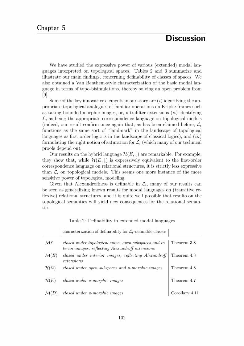
We have studied the expressive power of various (extended) modal lan-guages interpreted on topological spaces. Tables 2 and 3 summarize andillustrate our main findings, concerning definability of classes of spaces. Wealso obtained a Van Benthem-style characterization of the basic modal lan-guage in terms of topo-bisimulations, thereby solving an open problem from[9].

Some of the key innovative elements in our story are (i) identifying the ap-propriate topological analogues of familiar operations on Kripke frames suchas taking bounded morphic images, or, ultrafilter extensions (ii) identifyingLt as being the appropriate correspondence language on topological models(indeed, our result confirm once again that, as has been claimed before, Lt

functions as the same sort of “landmark” in the landscape of topologicallanguages as first-order logic is in the landscape of classical logics), and (iii)formulating the right notion of saturation for Lt (which many of our technicalproofs depend on).

Our results on the hybrid language H(E, ↓) are remarkable. For example,they show that, while H(E, ↓) is expressively equivalent to the first-ordercorrespondence language on relational structures, it is strictly less expressivethan Lt on topological models. This seems one more instance of the moresensitive power of topological modeling.

Given that Alexandroffness is definable in Lt, many of our results canbe seen as generalizing known results for modal languages on (transitive re-flexive) relational structures, and it is quite well possible that results on thetopological semantics will yield new consequences for the relational seman-tics.

Table 2: Definability in extended modal languages

characterization of definability for Lt-definable classes

ML closed under topological sums, open subspaces and in-

terior images, reflecting Alexandroff extensions

Theorem 3.8

M(E) closed under interior images, reflecting Alexandroff

extensions

Theorem 4.3

H(@) closed under open subspaces and u-morphic images Theorem 4.8

H(E) closed under u-morphic images Theorem 4.7

M(D) closed under u-morphic images Corollary 4.11

102

Chapter 5

Discussion

Table 3: Properties of topological spaces definable in various languages

Lt M M(E) H(@) H(E) (or M(D))

T0∀xy.(x 6= y →

∃Ux.(y 6εU) ∨ ∃Vy.(x 6ε V ))no no

@i3j ∧ @j3i

→ @ijidem

T1 ∀xy.(x 6= y → ∃Ux.(y 6εU)) no no 3i → i idem

T2∀xy.(x 6= y →

∃Ux.∃Vy.∀z.(z 6εU ∨ z 6ε V ))no no no no

Density-in-itself

∀x∀Ux(∃y 6= x(y ∈ U)) no no 3¬i idem

Connectedness no noA(2p ∨ 2¬p)→ Ap ∨ A¬p

no as in M(E)

Hereditaryirresolvability

no2(2(p → 2p) → p)

→ 2pidem idem idem

103

We finish by mentioning interesting directions for future research.

• Correspondence theory for alternative semantics. There are atleast two other semantic paradigms where the approach taken in thispaper might prove useful. We discuss them briefly.

Diamond as derived set operator. For any subset S of a topologicalspace, the derived set dS is the set of limit points of S, i.e., all points xof which each open neighborhood contains an element of S distinct fromx itself. The closure operator can be defined in terms of the derivedset operator: CS = S ∪ dS. The converse does not hold, as d isstrictly more expressive than C [28, 5]. Indeed, if we interpret the ¨ asthe derived set operator, then the modal formula ¨⊤ defines density-in-itself. With the derived set operator we can also partially mimicnominals: p∧¬¨p expresses that, within small enough neighborhoods,p acts as a nominal for the current point. Conversely, with nominals wecan partially mimic the d-operator: @i(¨φ ↔ 3(φ∧¬i)) is valid. Theprecise connection between d and nominals remains to be investigated.The standard translation should be modified in the following way toaccount for the new semantics:

STx(¨φ) := ∀U.(xεU → ∃y.(yεU ∧ x 6= y ∧ STy(φ)))

This is still a Lt-formula. Whether or not the expressive power of thecorresponding fragment of Lt can be characterized in a way we havepresented here remains to be seen. The interested reader is referred to[13, 28, 5] for more details on this topological semantics.

Neighborhood semantics. This is a generalization of the topologi-cal semantics for modal logic that allows to tackle non-normal modallogics. The corresponding structures are neighborhood frames (W,n)where W is a non-empty set and n ⊆ W×℘(W ) is a binary relationbetween points of W and subsets of W . The correspondence theoryfor Monotonic modal logic has been explored in [20] and analogues ofthe Goldblatt-Thomason theorem and the Van Benthem theorem havebeen proved for the neighborhood semantics. Quite general definabil-ity results are also put forth in [24] using the co-algebraic approach.We believe that a modification of the approach presented in this paperwill further strengthen the investigation of the precise expressive powerof non-normal modal logics over neighborhood frames. We outline onepossible route in this direction that is similar to, but more general than,the one pursued in [20].

Extend the language L2 by another intersorted binary relation symbolη. To ensure that ε behaves like the membership relation we postulate

∀U, V.(U = V ↔ ∀x.(xεU ↔ xεV ))

The models for this new language L2η are of the form (X, σ, ν) with X a

set and σ ⊆ ℘X. The relation ε is interpreted as set-theoretic member-ship, while the interpretation of η defines a relation between elements

104

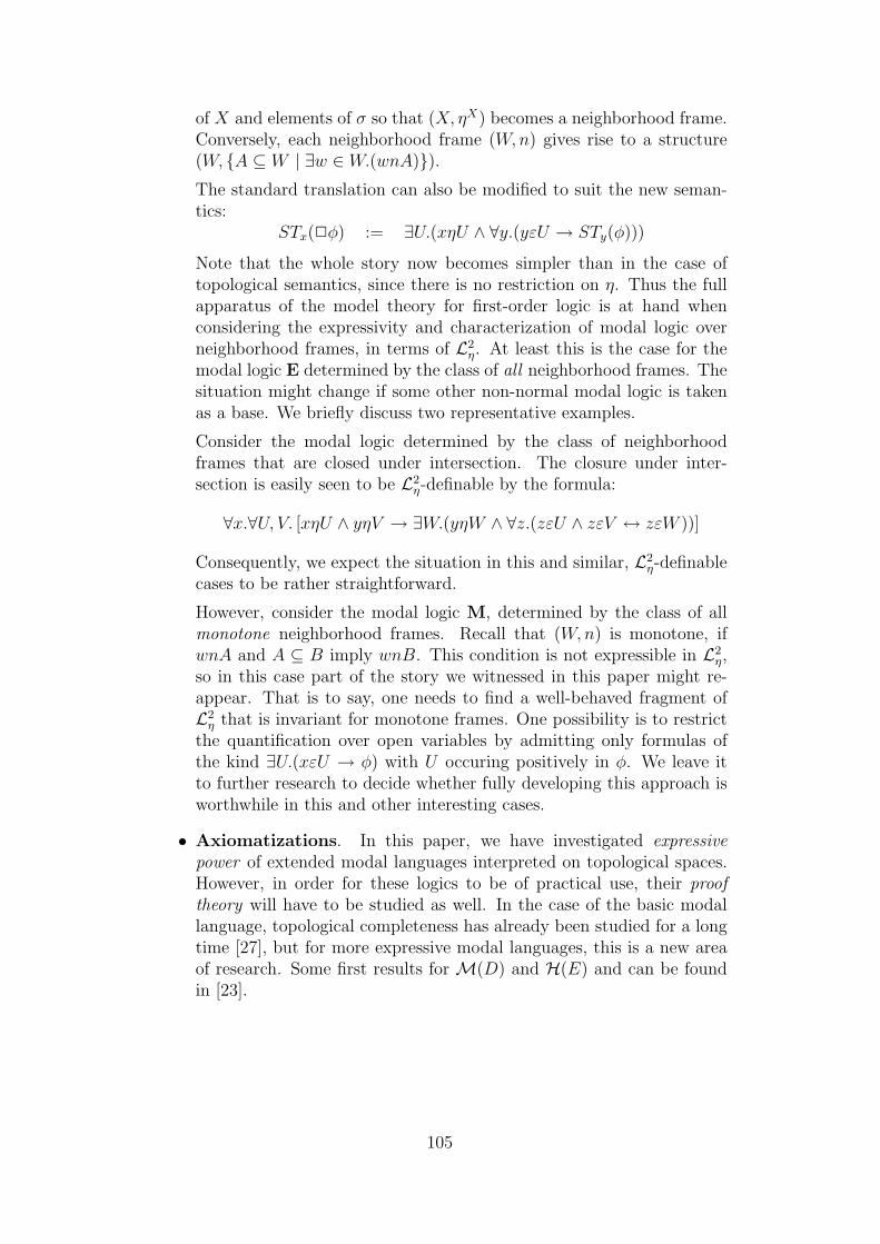
of X and elements of σ so that (X, ηX) becomes a neighborhood frame.Conversely, each neighborhood frame (W,n) gives rise to a structure(W, {A ⊆ W | ∃w ∈ W.(wnA)}).

The standard translation can also be modified to suit the new seman-tics:

STx(2φ) := ∃U.(xηU ∧ ∀y.(yεU → STy(φ)))

Note that the whole story now becomes simpler than in the case oftopological semantics, since there is no restriction on η. Thus the fullapparatus of the model theory for first-order logic is at hand whenconsidering the expressivity and characterization of modal logic overneighborhood frames, in terms of L2

η. At least this is the case for themodal logic E determined by the class of all neighborhood frames. Thesituation might change if some other non-normal modal logic is takenas a base. We briefly discuss two representative examples.

Consider the modal logic determined by the class of neighborhoodframes that are closed under intersection. The closure under inter-section is easily seen to be L2

η-definable by the formula:

∀x.∀U, V. [xηU ∧ yηV → ∃W.(yηW ∧ ∀z.(zεU ∧ zεV ↔ zεW ))]

Consequently, we expect the situation in this and similar, L2η-definable

cases to be rather straightforward.

However, consider the modal logic M, determined by the class of allmonotone neighborhood frames. Recall that (W,n) is monotone, ifwnA and A ⊆ B imply wnB. This condition is not expressible in L2

η,so in this case part of the story we witnessed in this paper might re-appear. That is to say, one needs to find a well-behaved fragment ofL2

η that is invariant for monotone frames. One possibility is to restrictthe quantification over open variables by admitting only formulas ofthe kind ∃U.(xεU → φ) with U occuring positively in φ. We leave itto further research to decide whether fully developing this approach isworthwhile in this and other interesting cases.

• Axiomatizations. In this paper, we have investigated expressivepower of extended modal languages interpreted on topological spaces.However, in order for these logics to be of practical use, their prooftheory will have to be studied as well. In the case of the basic modallanguage, topological completeness has already been studied for a longtime [27], but for more expressive modal languages, this is a new areaof research. Some first results for M(D) and H(E) and can be foundin [23].

105

[1] M. Aiello and J. van Benthem. Logical patterns in space. In D. Barker-Plummer, D. Beaver, J. van Benthem, and P. Scotto di Luzio, editors,Words, Proofs, and Diagrams, pages 5–25. CSLI Stanford, 2002.

[2] S. Artemov, J. Davoren, and A. Nerode. Modal logics and topologicalsemantics for hybrid systems, 1997.

[3] J. van Benthem. Modal formulas are either elementary or not Σ∆-elementary. Journal of Symbolic Logic, 41(2):436–438, 1976.

[4] J. van Benthem, G. Bezhanishvili, B. ten Cate, and D. Sarenac. Multi-modal logics of products of topologies. Studia Logica, 2006. to appear.

[5] G. Bezhanishvili, L. Esakia, and D. Gabelaia. Some results on modalaxiomatization and definability for topological spaces. Studia Logica,81(3):325–355, 2005.

[6] G. Bezhanishvili, R. Mines, and P. Morandi. Scattered, Hausdorff-reducible, and hereditary irresolvable spaces. Topology and its Appli-cations, 132:291–306, 2003.

[7] G. Bezhanishvili, R. Mines, and P. Morandi. Topo-canonical completionsof closure algebras and heyting algebras. Algebra Universalis, 2006.accepted.

[8] P. Blackburn, M. de Rijke, and Y. Venema. Modal Logic. CambridgeUniversity Press, 2001.

[9] P. Blackburn and J. van Benthem. Modal logic: a semantic perspective.

[10] B. ten Cate. Model theory for extended modal languages. PhD thesis,University of Amsterdam, 2005. ILLC Dissertation Series DS-2005-01.

[11] C. C. Chang and H. J. Keisler. Model Theory. North Holland, Amster-dam, third edition edition, 1989.

[12] R. Engelking. General Topology. Polish Scientific Publishers, Warszawa,1977.

[13] L. Esakia. Diagonal constructions, Lob’s formula and Cantor’s scat-tered spaces. In Logical and Semantical Investigations, pages 128–143.Academy Press, Tbilisi, 1981. In Russian.

[14] L. Feng and O. Masaveu. Exactly n-resolvable spaces and ω-resolvability.Math. Japonica, 50(3):333–339, 1999.

106

Bibliography

[15] J. Flum and M. Ziegler. Topological Model Theory. Springer-Verlag,Berlin, 1980.

[16] S. Garavaglia. Model theory of topological structures. Annals of Math-ematical Logic, 14:13–37, 1978.

[17] G. Gargov and V. Goranko. Modal logic with names. Journal of Philo-sophical Logic, 22:607–636, 1993.

[18] M. Gehrke, J. Harding, and Y. Venema. Macneille completions andcanonical extensions. Transactions of the American Mathematical Soci-ety, 358:573–590, 2006.

[19] R. Goldblatt. First-order definability in modal logic. Journal of SymbolicLogic, 40(1):35–40, 1975.

[20] H. H. Hansen. Monotonic modal logics. Master’s thesis, ILLC, Univer-sity of Amsterdam, 2003.

[21] B. Konev, R. Kontchakov, F. Wolter, and M. Zakharyaschev. On dy-namic topological and metric logics. Studia Logica, 2006. to appear.

[22] P. Kremer and G. Mints. Dynamic topological logic. Ann. Pure Appl.Logic, 131(1-3):133–158, 2005.

[23] A. Kudinov. Topological modal logics with difference modality. InI. Hodkinson G. Governatori and Y. Venema, editors, Advances in ModalLogic, volume 6, pages 319–332. College Publications, London, 2006.

[24] A. Kurz. The Goldblatt-Thomason theorem for coalgebras. manuscript,2006.

[25] T. Litak. On the Gargov-Goranko translation. Under submission.

[26] J. Makowsky and M. Ziegler. Topological model theory with an in-terior operator: consistency properties and back-and-forth arguments.Arch.Math.Logic, 21(1):37–54, 1981.

[27] J.C.C. McKinsey and A. Tarski. The algebra of topology. Annals ofMathematics, 45:141–191, 1944.

[28] V. Shehtman. “Everywhere” and “Here”. Journal of Appplied Non-Classical Logic, 9:369–380, 1999.

107

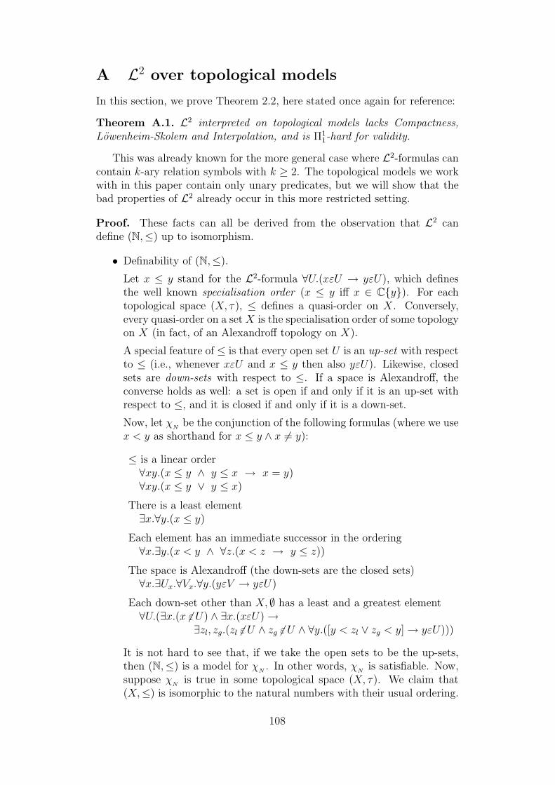
A L2 over topological models

In this section, we prove Theorem 2.2, here stated once again for reference:

Theorem A.1. L2 interpreted on topological models lacks Compactness,Lowenheim-Skolem and Interpolation, and is Π1

1-hard for validity.

This was already known for the more general case where L2-formulas cancontain k-ary relation symbols with k ≥ 2. The topological models we workwith in this paper contain only unary predicates, but we will show that thebad properties of L2 already occur in this more restricted setting.

Proof. These facts can all be derived from the observation that L2 candefine (N,≤) up to isomorphism.

• Definability of (N,≤).

Let x ≤ y stand for the L2-formula ∀U.(xεU → yεU), which definesthe well known specialisation order (x ≤ y iff x ∈ C{y}). For eachtopological space (X, τ), ≤ defines a quasi-order on X. Conversely,every quasi-order on a set X is the specialisation order of some topologyon X (in fact, of an Alexandroff topology on X).

A special feature of ≤ is that every open set U is an up-set with respectto ≤ (i.e., whenever xεU and x ≤ y then also yεU). Likewise, closedsets are down-sets with respect to ≤. If a space is Alexandroff, theconverse holds as well: a set is open if and only if it is an up-set withrespect to ≤, and it is closed if and only if it is a down-set.

Now, let χN

be the conjunction of the following formulas (where we usex < y as shorthand for x ≤ y ∧ x 6= y):

≤ is a linear order∀xy.(x ≤ y ∧ y ≤ x → x = y)∀xy.(x ≤ y ∨ y ≤ x)

There is a least element∃x.∀y.(x ≤ y)

Each element has an immediate successor in the ordering∀x.∃y.(x < y ∧ ∀z.(x < z → y ≤ z))

The space is Alexandroff (the down-sets are the closed sets)∀x.∃Ux.∀Vx.∀y.(yεV → yεU)

Each down-set other than X, ∅ has a least and a greatest element∀U.(∃x.(x 6εU) ∧ ∃x.(xεU) →

∃zl, zg.(zl 6εU ∧ zg 6εU ∧ ∀y.([y < zl ∨ zg < y] → yεU)))

It is not hard to see that, if we take the open sets to be the up-sets,then (N,≤) is a model for χ

N. In other words, χ

Nis satisfiable. Now,

suppose χN

is true in some topological space (X, τ). We claim that(X,≤) is isomorphic to the natural numbers with their usual ordering.

108

To prove this, it suffices to show that, for any w ∈ X, the set {v | v ≤w} is finite (this property, together with the fact that ≤ is a linear orderand each element has an immediate successor, characterizes the naturalnumbers up to isomorphism). In other words, we need to demonstratethat no infinite ascending or descending chains exist below an arbitrarypoint of X.

Suppose that for some w ∈ X the set (w] = {v ∈ X | v ≤ w} containsan infinite ascending chain A= {a1, a2, . . . } with ai<ai+1 for each i ∈ N.Consider the down-set (A] = {w ∈ X | ∃ai ∈ A.(w ≤ ai)} generated bythe set A. Since (A] ⊆ (w], we know that (A] 6= X, and hence there isa greatest element g ∈ (A]. By the definition of (A], we have g ≤ ai forsome i ∈ N. By definition of A, we also have ai < ai+1 and so g < ai+1,contradicting the maximality of g in (A]. Hence no infinite ascendingchains exist below w.

Next, suppose that for some w ∈ X the set (w] = {v ∈ X | v ≤ w}contains an infinite descending chain D = {d1, d2, . . . } , with di+1 < di

for each i ∈ N. Then the set X \ [D) = {w ∈ X | ∀di ∈ D.(w < di)} isa non-empty down-set (for non-emptyness, note that the least elementof X cannot belong to D, and hence belongs to X \ [D)). But then,there must be a greatest element g ∈ X \ [D). Let g′ be the immediatesuccessor of g. Note that by maximality of g we must have di ≤ g′ forsome i ∈ N. By definition of D, di+1 < di and we obtain di+1 ≤ g,hence g ∈ [D), a contradiction. Thus no infinite descending chainsexist below w.

• Failure of Compactness

Consider the following set of L2-sentences with one unary predicate P :

Γ ≡ {χN,∃x.P (x)} ∪ {ϕn | n ∈ N}

where ϕk ≡ ∀x.(P (x) → ∃y1, . . . , yk.(y1 < y2 < . . . < yk < x) expressthat every point in P has at least k predecessors. Every finite subsetof Γ is satisfiable but Γ itself is not.

In fact, it is possible to show failure of compactness even without usingany unary predicates.

• Failure of upward and downward Lowenheim-Skolem

Since χN

characterizes (N,≤) up to isomorphism, clearly, it has onlycountable models. Thus, the upward Lowenheim-Skolem theorem failsfor L2. The downwards Lowenheim-Skolem theorem fails as well: wecan easily express in L2

= that the specialisation order ≤ is a dense linearordering without endpoints. Further, we can express (on Alexandroffspaces) that each non-empty up-set has an infimum:

Inf ∀U.(∃x.(xεU) → ∃y.∀z. ((y < z → zεU) ∧ (zεU → y ≤ z))

)

Combining these formulas, we can enforce a complete dense linear orderwithout endpoints. An example of an infinite model satisfying this is

109

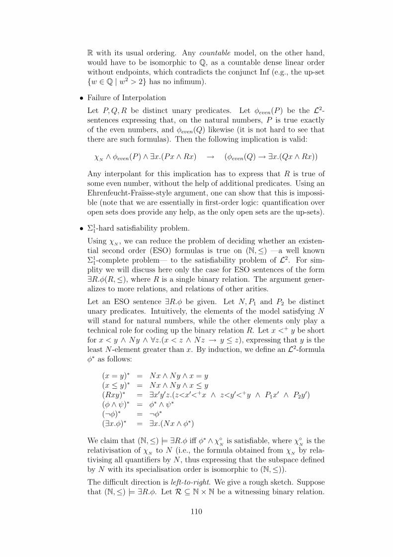
R with its usual ordering. Any countable model, on the other hand,would have to be isomorphic to Q, as a countable dense linear orderwithout endpoints, which contradicts the conjunct Inf (e.g., the up-set{w ∈ Q | w2 > 2} has no infimum).

• Failure of Interpolation

Let P, Q,R be distinct unary predicates. Let φeven(P ) be the L2-sentences expressing that, on the natural numbers, P is true exactlyof the even numbers, and φeven(Q) likewise (it is not hard to see thatthere are such formulas). Then the following implication is valid:

χN∧ φeven(P ) ∧ ∃x.(Px ∧ Rx) → (φeven(Q) → ∃x.(Qx ∧ Rx))

Any interpolant for this implication has to express that R is true ofsome even number, without the help of additional predicates. Using anEhrenfeucht-Fraısse-style argument, one can show that this is impossi-ble (note that we are essentially in first-order logic: quantification overopen sets does provide any help, as the only open sets are the up-sets).

• Σ11-hard satisfiability problem.

Using χN, we can reduce the problem of deciding whether an existen-

tial second order (ESO) formulas is true on (N,≤) —a well knownΣ1

1-complete problem— to the satisfiability problem of L2. For sim-plity we will discuss here only the case for ESO sentences of the form∃R.φ(R,≤), where R is a single binary relation. The argument gener-alizes to more relations, and relations of other arities.

Let an ESO sentence ∃R.φ be given. Let N, P1 and P2 be distinctunary predicates. Intuitively, the elements of the model satisfying Nwill stand for natural numbers, while the other elements only play atechnical role for coding up the binary relation R. Let x <+ y be shortfor x < y ∧ Ny ∧ ∀z.(x < z ∧ Nz → y ≤ z), expressing that y is theleast N -element greater than x. By induction, we define an L2-formulaφ∗ as follows:

(x = y)∗ = Nx ∧ Ny ∧ x = y(x ≤ y)∗ = Nx ∧ Ny ∧ x ≤ y(Rxy)∗ = ∃x′y′z.(z<x′<+x ∧ z<y′<+y ∧ P1x

′ ∧ P2y′)

(φ ∧ ψ)∗ = φ∗ ∧ ψ∗

(¬φ)∗ = ¬φ∗

(∃x.φ)∗ = ∃x.(Nx ∧ φ∗)

We claim that (N,≤) |= ∃R.φ iff φ∗ ∧χ◦N

is satisfiable, where χ◦N

is therelativisation of χ

Nto N (i.e., the formula obtained from χ

Nby rela-

tivising all quantifiers by N , thus expressing that the subspace definedby N with its specialisation order is isomorphic to (N,≤)).

The difficult direction is left-to-right. We give a rough sketch. Supposethat (N,≤) |= ∃R.φ. Let R ⊆ N × N be a witnessing binary relation.

110

Now, we define our model for φ∗ ∧ χ◦N

as follows: the subspace definedby N is simply the Alexandroff topology generated by (N,≤). For eachpair (m,n) ∈ R, we create three distinct ¬N -elements, (m,n)0, (m, n)1

and (m,n)2. Then we make sure that m is the least N -successor of(m,n)1 and P1 holds at (m,n)1, n is the least N -successor of (m,n)2 andP2 holds at (m,n)2, (m,n)0 < (m,n)1 and (m,n)0 < (m,n)2. In thisway, we ensure that, for any pair of natural numbers m,n, (m,n) ∈ Riff the L2-formula (Rxy)∗ is true of (m,n) in the constructed model.Once this observation is made, the claim becomes easy to prove.

⊣

111

B General Topology

In this appendix we try to gather the definitions from general topology usedthroughout the thesis. Most of the material exposed here is based on thesource [12].

B.0.1 Topological spaces

A topological space X = 〈X, τ〉 is a nonempty set X together with the col-lection of its open subsets τ ⊆ ℘(X) closed under finite meets and arbitraryjoins. If x ∈ X and x ∈ O ∈ τ then O is said to be an open neighbourhood

of x. For a subset A ⊆ X the topology induced by τ can be defined asτA = {O ∩ A | O ∈ τ}. Then A = 〈A, τA〉 is called a subspace of X.

The simplest example of a topological space is the one point spaceX = {x} with the only possible topology {∅, X}. In general on any nonemptyset X one can define two topologies—the trivial topology {∅, X} and thediscrete topology ℘(X). A bit more interesting is the topology of the Sier-

pinski space 〈{a, b} , {∅, a, {a, b}}〉. The real line R is another example ofa topological space in which open sets are arbitrary unions of open intervals(x, y).

In general arbitrary intersections of open sets need not be open. Spaces inwhich the intersection of opens is always an open set are called Alexandroff

spaces. In particular, any finite topological space is Alexandroff.A topology τ ′ on a set X is aid to be finer than the topology τ on the

same set if τ ⊆ τ ′. It is also said that τ ′ extends τ or that τ is coarser

than τ ′.

B.0.2 Closure, interior and derived set operators

For a subset A ⊆ X its interior IA is defined as the largest open set con-tained in A. More precisely:

IA =⋃

{O | O ⊆ A, O ∈ τ}

Dually, the closure CA of a set A ⊆ X is defined as the smallest closedset containing A, where by a closed set we mean a set that has the opencomplement. Alternative ways of defining a topological space is to pose cer-tain (Kuratowski) axioms which the operators of closure and interior shouldsatisfy. In particular, X = 〈X, C〉 is said to be a topological space, if thefollowing hold for arbitrary subsets of X:

(C1) C∅ = ∅,

(C2) A ⊆ CA,

(C3) C(A ∪ B) = CA ∪ CB,

(C4) CCA = CA.

Dually, X = 〈X, I〉 is said to be a topological space, if the following holdfor arbitrary subsets of X:

112

(I1) IX = X,(I2) IA ⊆ A,(I3) I(A ∩ B) = IA ∩ IB,(I4) IIA = IA.

If the closure operator C satisfying the above conditions is given, thenthe interior operator can be defined as IA ≡ (CAc)c. Saying that A is openiff A = IA defines the collection τ = {A ⊆ X | A = IA} which qualifies fortopology and induces the very same interior operators I and C. Dually, A isclosed iff A = CA. Both closure and interior operators are monotone, thatis if A ⊆ B then CA ⊆ CB and IA ⊆ IB. Another monotone operator is aderived set operator . For a subset A ⊆ X of a topological space A is thecollection of all limit points of A, where x ∈ X is said to be a limit point

of A if for every open neighbourhood O ∈ τ of x the set O ∩ A contains apoint y such that x 6= y. Formally

A = {x ∈ X | ∀O ∈ τ(x ∈ O → (O − {x}) ∩ A 6= ∅)}

The derived set operator satisfies the following axioms in an arbitrary topo-logical space:

(D1) ∅ = ∅,(D2) (A ∪ B) = A ∪ B,(D3) A ⊆ A ∪ A.

The connection between C and is expressed in the following equationvalid in an arbitrary topological space

CA = A ∪ A

B.0.3 Resolvable and irresolvable spaces

A subset A ⊆ X is dense-in-itself if A ⊆ A. A space X that is dense-in-itself is also sometimes called crowded. More generally, a set A ⊆ Xis said to be dense in a set B ⊆ X if A ⊆ B. A subset A ⊆ X is calledeverywhere dense if CA = X. A space X that can be decomposed into twodisjoint dense subsets is called resolvable. Spaces that are not resolvable arecalled irresolvable. We say that a space X is hereditarily irresolvable

(or HI for short), if its every subspace is irresolvable. A subset A ⊆ X of atopological space is called nowhere dense if ICA = ∅.

B.0.4 Scattered spaces and the Cantor-Bendixson Theorem

A point x ∈ X is called an isolated point of A if x is not a limit point of A. Inother words, x is an isolated point of A if there exists an open neighbourhoodO ∈ τ of x such that O∩A ⊆ {x}. A point x ∈ X is an isolated point (of X)if {x} ∈ τ . A subset A ⊆ X of a space X is called discrete if every x ∈ Ais an isolated point of A. A space X is called scattered if every subspaceof X has an isolated point. A space is called weakly scattered if the set ofall isolated points is everywhere dense. A subset A ⊆ X is called perfect ifA is closed and dense-in-itself.

113

Theorem B.1 (Cantor-Bendixson). An arbitrary topological space X can

be decomposed into the union of two disjoint subspaces P and S such that Pis perfect and S is scattered.

B.0.5 Separation axioms

A space X is said to satisfy the T0 separation axiom if for any two distinctpoints in X there exists an open set which contains one of them, but not theother. A space satisfies T1 separation axiom if for any two distinct pointsx, y ∈ X there exists an open neighbourhood O of x such that y /∈ O. Theequivalent characterization of T1 spaces is that every singleton set is closed.A space is called Hausdorff if any two distinct points have disjoint openneighbourhoods. A space X is said to satisfy TD separation axiom if everysingleton can be obtained as the intersection of an open a closed subsets ofX. It is known that every Hausdorff space is T1, every T1 space is TD andevery TD space is T0

B.0.6 Connectedness and disconnectedness

A topological space X is called connected if the only closed and open subsetsof X are ∅ and X. A space is called well-connected if for any two opensubsets O1, O2 ∈ τ , O1 ∪ O2 = X implies O1 = X or O2 = X. X is said tobe extremally disconnected if the closure of any open subset is open. Aspace is perfectly disconnected if it is T0 and for any two disjoint subsetsA ∩ B = ∅ we have A ∩ B = ∅.

B.0.7 Maps between spaces

A map f : X → Y between the topological space X and Y is called con-

tinuous if f−1(O) ⊆ X is open whenever O ⊆ Y is open (pre-image of anyopen is open). A map f : X → Y is called open if f(O) ⊆ Y is openwhenever O ⊆ X is open (image of any open is open). A map f : X → Y isan homeomorphism if it is a bijective open continuous map, that is if f isinjective, onto and it is continuous together with its inverse.

114

Model theory for extensions of modal logic -...

Documents

Transcript of Model theory for extensions of modal logic -...