Model Simpliﬁcation via Super Elements using the …GeoandEnvironmentalEngineering...

Faculty of Civil, Geo and Environmental Engineering

Chair for Computation in Engineering

Prof. Dr. rer. nat. Ernst Rank

Model Simplification via Super Elements

using the Finite Cell Method

Martin Ruchti

Bachelor’s thesis

for Engineering Science (Bachelor of Science Program)

Author: Martin Ruchti

Matriculation number: 03620819

Supervisors: Prof. Dr.rer.nat. Ernst Rank

Nils Zander, M.Sc.

Dipl.-Ing. Tino Bog

Date of issue: 15th June 2013

Date of submission: 11th September 2013

Involved Organisations

Chair for Computation in EngineeringFaculty of Civil, Geo and Environmental EngineeringTechnische Universitat MunchenArcisstraße 21D-80333 Munchen

Declaration

With this statement, I declare that I have independently completed this Bachelor’s thesis.The thoughts taken directly or indirectly from external sources are properly marked as such.This thesis was not previously submitted to another academic institution and has also notyet been published.

Munchen, 11th September 2013

Martin Ruchti

Martin RuchtiChristof Probst Str. 16D-80805 Munchene-Mail: [email protected]

Abstract

In this bachelor’s thesis, the theory and the application of the super element approach inthe Finite Cell Method is given. Furthermore, an implementation in the FCM frameworkAdhoC++, which was developped by the chair of Computation in Engineering of the Tech-nische Universitat Munchen is introduced. For simplicity, linear elasticity, static analysis andtwo-dimensionality are assumed. For generating super elements, weak constraints are used.The program developped as part of this thesis is analyzed by several tests, comparing resultsfrom a classical mesh patch test with results from a super element, obtained by patchingmeshes involving a reduced mesh.

Abstract

In dieser Bachelorarbeit wird die Theorie und die Anwendung der Superelement Idee, inder Finite Zellen Methode beschrieben. Des Weiteren wird eine Implementierung im FCMProgramm AdhoC++, das vom Lehrstuhl fur Computation in Engineering der TechnischenUniversitat Munchen entwickelt wurde, vorgestellt. Der Einfachheit halber sind lineare Elas-tizitat, Statik und Zweidimensionalitat vorrausgesetzt. Um Super Elemente zu generieren,werden schwache Zwangsbedingung (constraints) verwandt. Zur Analyse des Programms, dasals Teil dieser Arbeit entwickelt wurde, werden mehrere Test betrachtet. Diese vergleichendie Losung eines klassischen Patch-Tests mit der Losung aus einem Superelement, das durchdie Vernahung eines reduzierten Gitters mit mehreren nicht reduzierten Gittern entsteht.

VII

Contents

1 Introduction 1

1.1 Scope of this Work . . . . . . . . . . . . . . . . . . . . . . . . . . . . . . . . . 2

1.2 Nomenclature . . . . . . . . . . . . . . . . . . . . . . . . . . . . . . . . . . . . 4

2 The Finite Cell Method 7

2.1 Motivation . . . . . . . . . . . . . . . . . . . . . . . . . . . . . . . . . . . . . 7

2.2 General Principle . . . . . . . . . . . . . . . . . . . . . . . . . . . . . . . . . . 8

2.3 High Order Ansatz Functions . . . . . . . . . . . . . . . . . . . . . . . . . . . 10

2.4 The Fictitious Domain Approach . . . . . . . . . . . . . . . . . . . . . . . . . 11

2.5 Adaptive Integration . . . . . . . . . . . . . . . . . . . . . . . . . . . . . . . . 13

2.6 Dirichlet Boundary Conditions . . . . . . . . . . . . . . . . . . . . . . . . . . 13

2.6.1 Penalty Method . . . . . . . . . . . . . . . . . . . . . . . . . . . . . . 15

2.6.2 Nitsche’s Method . . . . . . . . . . . . . . . . . . . . . . . . . . . . . . 16

3 Model Reduction 17

3.1 Guyan - Irons Reduction . . . . . . . . . . . . . . . . . . . . . . . . . . . . . . 17

3.2 Dynamic Reduction . . . . . . . . . . . . . . . . . . . . . . . . . . . . . . . . 19

3.3 Possible Sources of Error for Reduction . . . . . . . . . . . . . . . . . . . . . 19

4 Weakly Imposed Constraints 21

4.1 Penalty Method . . . . . . . . . . . . . . . . . . . . . . . . . . . . . . . . . . . 22

4.2 Nitsche’s Method . . . . . . . . . . . . . . . . . . . . . . . . . . . . . . . . . . 22

4.3 Use of Constraints in Super Elements . . . . . . . . . . . . . . . . . . . . . . 22

5 Implementation 25

5.1 Program Terminology . . . . . . . . . . . . . . . . . . . . . . . . . . . . . . . 25

5.2 Reduction . . . . . . . . . . . . . . . . . . . . . . . . . . . . . . . . . . . . . . 26

5.2.1 Pseudo Code - Reduction . . . . . . . . . . . . . . . . . . . . . . . . . 27

5.3 Condensed Mesh Creation . . . . . . . . . . . . . . . . . . . . . . . . . . . . 28

5.3.1 Pseudo Code - Condensed Mesh Creation . . . . . . . . . . . . . . . . 28

5.4 Mixed Super Elements . . . . . . . . . . . . . . . . . . . . . . . . . . . . . . . 29

5.4.1 Pseudo Code - Mixed Super Elements . . . . . . . . . . . . . . . . . . 29

6 Examples 31

6.1 Generic Setup . . . . . . . . . . . . . . . . . . . . . . . . . . . . . . . . . . . . 31

6.1.1 Analytic Solution . . . . . . . . . . . . . . . . . . . . . . . . . . . . . . 31

6.1.2 Error Declaration . . . . . . . . . . . . . . . . . . . . . . . . . . . . . . 33

6.2 Mesh Test with a Single Mesh . . . . . . . . . . . . . . . . . . . . . . . . . . . 33

6.2.1 Setup for One Mesh with 6× 2 Elements . . . . . . . . . . . . . . . . 336.2.2 Analytic Solution . . . . . . . . . . . . . . . . . . . . . . . . . . . . . . 346.2.3 Numerical Solution . . . . . . . . . . . . . . . . . . . . . . . . . . . . . 346.2.4 Discussion . . . . . . . . . . . . . . . . . . . . . . . . . . . . . . . . . . 35

6.3 Mesh Test with Three Patched Meshes . . . . . . . . . . . . . . . . . . . . . . 356.3.1 Setup for Three Meshes with 2× 2 Elements . . . . . . . . . . . . . . 356.3.2 Numerical Solution . . . . . . . . . . . . . . . . . . . . . . . . . . . . . 356.3.3 Discussion . . . . . . . . . . . . . . . . . . . . . . . . . . . . . . . . . . 37

6.4 Conform Mesh Test Involving a Condensed Mesh . . . . . . . . . . . . . . . . 376.4.1 Setup . . . . . . . . . . . . . . . . . . . . . . . . . . . . . . . . . . . . 376.4.2 Numeric Solution . . . . . . . . . . . . . . . . . . . . . . . . . . . . . . 376.4.3 Discussion . . . . . . . . . . . . . . . . . . . . . . . . . . . . . . . . . . 37

6.5 Non Conform Mesh Test Involving a Condensed Mesh . . . . . . . . . . . . . 376.5.1 Setup . . . . . . . . . . . . . . . . . . . . . . . . . . . . . . . . . . . . 386.5.2 Numeric Solution . . . . . . . . . . . . . . . . . . . . . . . . . . . . . . 38

6.6 Test of a Condensed Mesh from an Embedded Domain . . . . . . . . . . . . . 386.6.1 Setup . . . . . . . . . . . . . . . . . . . . . . . . . . . . . . . . . . . . 386.6.2 Numeric Solution . . . . . . . . . . . . . . . . . . . . . . . . . . . . . . 396.6.3 Discussion . . . . . . . . . . . . . . . . . . . . . . . . . . . . . . . . . . 39

6.7 Mesh with a Hole Test . . . . . . . . . . . . . . . . . . . . . . . . . . . . . . . 39

7 Conclusion 45

1

Chapter 1

Introduction

In engineering sciences, numerous problems lead to a partial differential equation (PDE). Ifthis equation is solved, the solution of the problem is achieved. Though, it can be challengingto find an analytical solution for the system of equations. Sometimes, even there is no suchsolution. To overcome this barrier, the Finite Element Method was introduced. It advancedto the standard tool in mechanics to solve the specific PDEs.However, since in the 60th, CPU and memory environments had poor performance and capac-ity, in comparison to nowadays, computer scientists had to worry about the size of equationsystems. For clarification, we can consider a super computer from 1965, the Control Data6600 which had a total high-speed memory of 1.3 mega bytes. Hence, scientists did researchon possibilities to reduce the overall size of stiffness and mass matrices for mechanical prob-lems, which then would fit into memory. Simultaneously, the techniques were designed topreserve accuracy as far as possible. The computational view is elaborately illustrated in[22]. Despite this strong relation to dynamics, the plurality of the principles can be appliedto statics, too. As for example, Zehn [22] points out, that it is promising for engineeringwork, to have precomputed standard parts. To accieve all the previous mentioned properties,the super element method was introduced.When we talk of super elements, we typically think of elements that are composed of numer-ous sub elements. This technique is closely linked to the substructure technique [2] or thecomponent mode synthesis [18] for dynamic analysis. Both are effective approaches to savecomputational power and to preserve flexibility at the same time.The method of creating and using super structures is an established concept in structuralstatics and dynamics. Introduced at the beginning of the 60th, most of the publications aimedat simplification in dynamic analysis. Scientists proved that systems of equations for com-plex structures can be simplified. Therefore, several reduction techniques were introduced byGuyan and Hurty [14], [18]. Furthermore, required coupling concepts where introduced byHurty and Bampton [19], [2] as well as studies on the accuracy and applicability of the abovementioned methods. The majority of scientists, who did research on super structures, weremembers of the aeronautic engineering. Therefore, most of the super element principles havean association to aircrafts and spacecrafts. The techniques were introduced for the sake ofcapability of solving complex dynamic structures on former computer systems.Since the beginning of super element methods, the motivation changed slightly. Due to theincreased capabilities of modern computers, the task mainly shifted from enabling the com-putation itself to the decrease of computational time. This is put into practice by means of

2 1. Introduction

parallelization. This way, many computational tasks can be carried out at once. Hence, superelements are of central interest again, since they provide a possibility to split the problem.The sub problems gained by this process can be computed at the same time. Especially inmarine engineering and in multi physics, sub structuring and hence, super elements, are ap-plied. For example, ship bodies are divided into sub structures to be able to carry out a morecomplex computation of critical parts [8]. In multi physics, the creation of e.g. thermal superelements is applied. This is done, to meet better approximations for the thermal behavior,while keeping the potential to solve on a personal computer [13]. This means, super elementconcepts are appropriate likewise for the use in CAD programs, on personal computers, togroup functional complexes. Accordingly, improved condensation algorithms are introducedand examined [10]. In addition, there are numerous approaches for automated creation ofsub and super structures [17].

Apparently, the development of super elements is impressive. However, most of the methodsbase on the Finite Element Method. Hence, the flexibility and adaptivity is limited. Thislimitation comes from the fact, that the Finite Element Method requires a mesh to carry outa computation. Additionally, in computational mechanics, models are often composed fromstructural elements like rods, beams or shells. These elements are highly effective, since theybase on substantial simplifications in kinematic and geometric properties. They reduce thedimension of the problem and hence, the computational effort of the solver. Applied in amodel, structural elements improve the speed of computation. However, bulky componentscannot be represented without substantial loss of the real behavior properties. This lack inflexibility and the absence of a bulk-like representation give a major drawback. To overcomethese limitation, it is desirable to be able to create super elements automatically, by theuse of the embedding domain approach. This way, it is possible to combine highly effectivestructural elements with precomputed structures, that reflect the mechanical behavior of abulk part. In addition, we gain flexibility and adaptivity by the use of the embedding domainapproach. This comes from the fact, that this technique does not require a mesh to representthe geometry anymore. However, such a technique does not exist, yet.

This thesis aims at closing this gap. For this purpose, the Finite Cell Method (FCM), re-cently developed by the Chair of Computation in Engineering [4], is used along with the superelement concept. The former, utilizes high order finite elements. The method simultaneouslypreserves flexibility, by automatically recovering the problem geometry during domain inte-gration. By the use of super elements along with the finite cell approach, we can gain highlyaccurate models with a reduced number of degrees of freedom, while preserving flexibilityand adaptivity.

1.1 Scope of this Work

In this thesis, the combination of the Finite Cell Method with the Super Element concept isexamined. Further, linear elasticity is assumed. As model problem, a two dimensional finitecell problem is considered. Therefore, the Finite Cell Method is explained, as well as theconcept of weak coupling and weak boundary conditions.For the sake of simplicity, only static analysis is considered. For understanding, the static

1.1. Scope of this Work 3

reduction technique is introduced and applied. An overview on the implementation is sub-sequently given and explained. Following, several examples probe the performance and ap-plicability of the combination of the Finite Cell Method, together with the super elementconcept.

4 1. Introduction

1.2 Nomenclature

In the following, an overview to the notation used in this thesis is given.

Ω Domain of the problemΩf Fictitious domainΩe Embedding domainΓ BoundaryΓN Neumann boundaryΓD Dirichlet boundaryΓI Interface boundaryσ Stress tensor

b Body load

t Tractionu Prescribed displacementC Constitutive tensorǫ Strain tensoru Displacementv Test functionf(u) Linear functionB(u, v) Bilinear functionN Shape functionsB Strain displacement matrixL L-OperatorK Stiffness matrixf Load vectoru Desired value for uuA/uB Displacement vectors that are coupledu(x, y) Displacement value at coordinates (x, y)σ(x, y) Stress value at coordinates (x, y)u(x, y) Exact displacement at coordinates (x, y)σ(x, y) Exact stress value at coordinates (x, y)N1D 1D Shape FunctionN2D 2D Shape FunctionN3D 3D Shape Functionui weighting function iKs Additional terms for the stiffness matrixKn Additional terms for the stiffness matrix∆x Grid size in x direction∆y Grid size in y directionα Factor for embedding domainui Independent degrees of freedomud Dependent degrees of freedomfi load vector of independent degrees of freedomfd load vector of dependent degrees of freedomkii Entry of the stiffness matrix for coupling an

independent degree of freedom with an independent one

1.2. Nomenclature 5

kid Entry of the stiffness matrix for coupling anindependent degree of freedom with a dependent one

kdd Entry of the stiffness matrix for coupling adependent degree of freedom with a dependent one

β Stabilization parameterΠC Function of potential energykred Reduced stiffness matrixfred Reduced load vectorered Set of reduced elementsecli Set of client elementsmred Set of reduced meshesmcli Set of client meshesvi vector of independent degrees of freedomvd vector of dependent degrees of freedomnDof Number of degrees of freedom

6 1. Introduction

7

Chapter 2

The Finite Cell Method

In this chapter, the fundamental concept of the Finite Cell Method is introduced. After ashort definition, the applicability of the Finite Cell Method is illustrated in an example tomotivate the use of this new tool in mechanical engineering. Following, the general principleof the Finite Element Method is presented. For the sake of faster convergence to the accurateresult, high order ansatz functions are introduced. Next, the fictitious domain approach isexplained. As a central part of the application of the Finite Cell Method, the concept ofadaptive integration is illustrated. Finally, boundary conditions are introduced.

The Finite Cell Method is a modification of the Finite Element Method. It combines thep-version of the Finite Element Method with the idea of embedding domains, which are alsoreferred to as fictitious domains. The Finite Cell Method was recently developed by the chairof Computation in Engineering [4]. The major advantage of this method is the expendabilityof mesh generation. This leads to a more flexible method to solve mechanical problems.There is no need for mesh generation, since the integration is done in an adaptive way byrecursively refining critical parts of the mechanical model. As mentioned by Duster et al. [4],the convergence to an accurate result is high.

2.1 Motivation

When having to solve a differential equations in multiple dimensions, we are typically notable to figure out an analytical solution for our problem, but have rather substantial problemseven to get an idea of how the solution would look like. To overcome this limitation, it ispossible to introduce an approximation function to solve the problem. The Finite ElementMethod is such a method. With the principle of a discrete and approximated solution, itis possible to convert the continuous problem to a system of equations which stems from adiscrete formulation of the problem. Once we have this system of equations, we can subse-quently solve it, using numerical schemes like Gaussian elimination.To introduce the discrete problem description, we need to discretize the domain first. Sub-sequently, we formulate the problem on the discrete domain and come up with a system ofequations, which are, in this thesis, linear. Since the solution depends on the discretization,it is a major issue in the Finite Element Method to create meshes for complex real world

8 2. The Finite Cell Method

applications. This task can become expensive and complicated.To overcome this barrier the Finite Cell Method uses the embedding domain idea. Follow-ing this approach, the actual domain is converted to a cartesian one. Once rectangular andcontinuous, the domain can easily be subdivided into smaller rectangles if a higher spatialresolution is required.

2.2 General Principle

At first, we will take a look at the theory of the Finite Element Method, since it provides thebasis for the Finite Cell Method.As a model problem we consider a domain Ω with a boundary Γ. To describe the responseof the domain to an external load we take a look at the equilibrium equation

∇ · σ + b = 0. (2.1)

Here, σ represents the stress tensor and b denotes the external load acting on the domain.We can now further rewrite σ as a new term

σ = C : ǫ (2.2)

to relate the stress σ to the strain ǫ. In this equation, C is the constitutive tensor, whichrepresents the material properties. Since we describe our system in terms of displacement wehave to find an expression for the strain, in terms of u. If we follow e.g. Hughes [9], we canrewrite 2.2 and come up with a dependence of ǫ on u.

ǫ =1

2[∇u+ (∇u)T ]. (2.3)

To describe the mechanical response of the domain to external loads and displacements wehave to introduce boundary conditions. If we look at figure 2.3, we can see two types ofboundary. The Neumann boundary or also called natural boundary is represented by ΓN . InContrast to that, ΓD represents the Dirichlet boundary on which a prescribed displacementis applied. We have to note, that these boundaries have additional properties by definition.

ΓN ∪ ΓD = Γ (2.4a)

ΓN ∩ ΓD = ∅ (2.4b)

This way we have either a Dirichlet or a Neumann boundary condition, but never both ofthem.Now having declared the two boundary types, we can continue in describing the equationsthat describe the mechanical response of our model problem. To enforce displacement andtraction on the boundary, we define our boundary conditions.

σ · n = t on ΓN (2.5a)

u = u on ΓD (2.5b)

Where t denotes the traction and u denotes the prescribed displacement.

2.2. General Principle 9

We can now write equation 2.1 in a weak form by inserting equations 2.2, 2.3, and 2.5 intothe first and applying the principle of virtual work, see Hughes [9]. We obtain the weakformulation of our partial differential equation.

∫

Ωǫ(v) : C : ǫ(u) dΩ =

∫

Ωv · b dΩ+

∫

ΓN

v · t dΓ (2.6)

Following up, we rewrite the equation above as

B(u, v) = f(v) (2.7)

Where B and f are defined as:

B(u, v) =

∫

Ωǫ(v) : C : ǫ(u) dΩ (2.8)

f(v) =

∫

Ωv · b dΩ+

∫

ΓN

v · t dΓ (2.9)

Herein, u is the solution function and v denotes an arbitrary test function. This equation forthe mechanical response is continuous. Solving this equation would be very expensive andsometimes not possible. However, the solution u can be represented as a linear combinationof functions. First we can write u as a infinite sum

u =∞∑

i=1

Niui, (2.10)

which exactly represents the solution as a linear combination of a infinite number of ansatzfunctions Ni weighted by a infinite number of weighting functions ui. We can now approxi-mate the solution as a linear combination of only a finite number of ansatz functions.

u =n∑

i=1

Niui (2.11)

Following a Bubnov-Galerkin approach, we use the same approximation for the test functionas well and obtain the new representation for v.

v =n∑

j=1

Nj vi (2.12)

The scheme of the following derivation is taken from Zander [20]. Inserting the new solutionand test functions into the equation 2.6 and using the fact, that

ǫ(u) = L ·N · u (2.13)

where L denote the linear differential operator, we obtain a new equation.

∫

Ω(L ·N · δv)TC(L ·N · u) dΩ =

∫

Ω(N · δv)T · b dΩ+

∫

ΓN

(N · δv)T · t dΓ (2.14)


We now rewrite (L ·N) = B and insert into 2.14 to obtain a shortened equation.

∫

ΩδvTBTCB · u dΩ =

∫

ΩNT · δvT · b dΩ+

∫

ΓN

NT · δvT · t dΓ (2.15)

In this equation we can subsequently factor out the δv.

δvT ·

∫

ΩBTCB · u dΩ = δvT ·

(∫

ΩNT · b dΩ+

∫

ΓN

NT · t dΓ

)

∀δvT ∈ V (2.16)

Since this equation has to hold for all δvT we can come up with

∫

ΩBTCB · u dΩ =

∫

ΩNT · b dΩ+

∫

ΓN

NT · t dΓ (2.17)

and subsequently with a reduced equation for our system

K · u = f , (2.18)

where we have replaced the left hand side and the right hand side in the following way

K =

∫

ΩBTCB dΩ (2.19a)

f =

∫

ΩNT · b dΩ+

∫

ΓN

NT · t dΓ (2.19b)

Now that we have finished the short derivation for the Finite Element Method, we can goon and point out the difference to the Finite Cell Method.

2.3 High Order Ansatz Functions

Until now, we had no exact look on the ansatz functions, used to obtain our solution andtest function approximation. In the following section they are explained.In the Finite Element Method, we mostly use linear ansatz functions. However, to get betterapproximations in the Finite Cell Method we use higher order ansatz functions. Additionally,we consider different types of ansatz functions. In this work, they are two-dimensional highorder ansatz functions. We have so-called nodal-modes, which correspond to the well-knownbilinear ansatz functions from the Finite Element Method. Nodal modes are one at thecorresponding node and zero at every other node. Furthermore, we have edge-modes, whichare a combination of a linear ansatz function in one direction with a higher order ansatzfunction in the other direction. Similar to the nodal modes, they are non-zero at the edgethey belong to and zero at every other edge in the element. Then, we have face-modes, whichare a combination of two higher order ansatz functions. Face modes are so-called internalmodes, since they are zero at every edge and every node, but non-zero at the correspondingface.All these two dimensional high order ansatz functions can be obtained from a tensor product.The tensor product aproach is the way in which to combine one dimensional high order ansatz

2.4. The Fictitious Domain Approach 11

Figure 2.1: The figure shows the tensor product for the two dimensional ansatz functions used inthe Finite Cell Method. [21]

functions to two dimensional ansatz functions. This can be written as

N2Dij = N1D(r) ·N1D(s). (2.20)

This tensor product can be seen in the figure 2.1. As in p-FEM, there are ansatz functionswith different order. Some ansatz functions can be seen also in 2.2.Using the Finite Cell Method, we come up with the same equation as 2.17 where we nowinsert the different ansatz functions N1D

i , N2Di , and N3D

i . u then consists of node degreesof freedom, edge degrees of freedom, and face degrees of freedom, each with its respectiveansatz function.

2.4 The Fictitious Domain Approach

Since, we need a spatial discretization to come up with 2.18, respectively 2.17, we have todiscretize our domain. The quality of the finite element solution heavily depends on theuniformness and smoothness of the spatial discretization. Therefore, we have to ensure theseproperties in our meshing process. This, however, can be very challenging if we consider adomain which is more complex than a regular rectangle. We then need special techniques formesh generation. In some cases a lot of time and computational effort is needed.To overcome this barrier, the Finite Cell Method was introduced by the chair of Computationin Engineering. It combines the finite element method with an approach which takes away


−10

1

−1

0

10

0.5

1

ξ1ξ2

(a) The figure shows the nodal

mode from the Finite Cell Method.

This mode corresponds to the bi-

linear form from the Finite Ele-

ment Method.

−10

1

−1

0

1

−0.8

−0.6

−0.4

−0.2

ξ1ξ2

(b) The figure then shows the low-

est order edge mode from the Fi-

nite Cell Method.

−10

1

−1

0

10

0.2

0.4

0.6

0.8

ξ1ξ2

(c) The figure shows the lowest or-

der face mode from the Finite Cell

Method.

Figure 2.2: The figures show the lowest order ansatz functions for the Finite Cell Method.

the need for a mesh. This simple but sophisticated technique is called fictitious domainapproach. The general idea of this technique is to embed the domain Ω, which in real worldproblems can be very complex, in an embedding domain Ωf of cartesian shape.

Ωe = Ω ∪ Ωf (2.21)

Where we can rewrite the fictitious domain in terms of the domain and its embedding domain.

Ωf = Ωe\Ω (2.22)

This setting is shown in the figure 2.5 and 2.4.Since we now deal with a rectangular domain, the meshing turns out to be trivial. We justhave to subdivide our domain into regular quadrilaterals of the size ∆x and ∆y. Thus, wehave to apply the second part of the fictitious domain approach, which extends the equation2.17 by an additional parameter α(x). The following section on the application of α refers tothe derivation by Duster et al. [4]

α(x) =

1.0 if x ∈ Ω

0.0 else.(2.23)

If we now write 2.17, we obtain an extended equation for B(u, v)

B(u, v) =

∫

Ωe

BT · αCB · u dΩe

=

∫

ΩBT · 1.0 · CB · u dΩ+

∫

Ωf

BT · 0.0 · CB · u dΩf

=

∫

ΩBTCB · u dΩe

(2.24)

2.5. Adaptive Integration 13

Following the same scheme, we can derive the new equation for the right hand side f(v)

f(v) =

∫

Ωe

NT · αb dΩe +

∫

ΓN

NT · t dΓ

= . . . =

∫

ΩNT · b dΩ+

∫

ΓN

NT · t dΓ.

(2.25)

Now we can write our equations 2.24 and 2.25 in matrix vector notation and obtain

Ke · ue = fe (2.26)

With this equation, we can now proceed like in Finite Element Method and solve our systemof linear equations.

2.5 Adaptive Integration

Starting with equation 2.17, we need an integration to obtain 2.26. This is done numerically.If we consider a common technique, like the trapezoidal rule, the Simpson’s rule integration orthe Gaussian quadrature, we consider a smooth function. However, we have a discontinuousfactor α. This is challenging, since we have to consider the fact, that we might integrateover some cells, that are cut by the boundary of the domain Ω. In this case, we require thepossibility to refine those cells. Using this refinement, we obtain a function α, that is smoothwithin the integration cells. Otherwise, the assumption of a smooth integrand does not holdanymore. However, in standard integration, refinement is typically not done locally, but isdone on the whole mesh.To meet locality requirements we integrate using an adaptive integration technique, likespace-tree partition. If we integrate adaptively, we check, if cells are cut by the boundaryΓ. For cut cells, we do an adaptive refinement. This is done recursively, until α is eitherconstant within the integration cell, or we reached the maximum refinement level. This way,we obtain a quad-tree for 2 dimensions, or a oct-tree for 3 dimensions. The procedure ofrecursive local refinement is shown in figure 2.6, taken from Schillinger et al. [16].

2.6 Dirichlet Boundary Conditions

In this section, the incorporation of Dirichlet boundary conditions in the Finite Cell Methodis illustrated.We need to apply Dirichlet boundary conditions, to force prescribed displacements. This isthe case, if we solve a mechanical problem, like a prestressed bar. We therefore set the dis-placement of one end of the bar to zero, while we set the other end of the bar to a prescribeddisplacement value.Since, in the Finite Cell Method, the pysical domain boundary is not resolved by the mesh,we need to find a method that implements Dirichlet boundary conditions, without the needof a conforming mesh discretisation. This is the case, if we apply Dirichlet boundary condi-tions in a weak sense. Since Neumann conditions are applied by a simple additional surfaceintegral in the weak formulation of the system, we do not consider this type of boundary


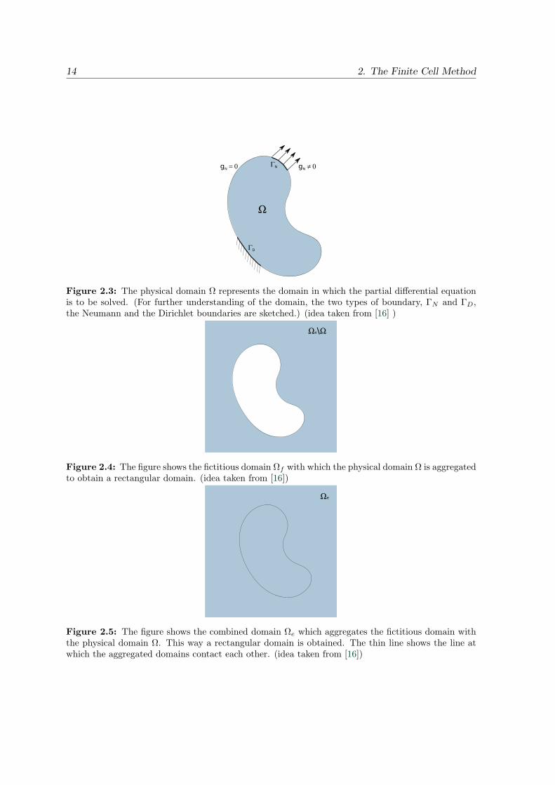
Figure 2.3: The physical domain Ω represents the domain in which the partial differential equationis to be solved. (For further understanding of the domain, the two types of boundary, ΓN and ΓD,the Neumann and the Dirichlet boundaries are sketched.) (idea taken from [16] )

Figure 2.4: The figure shows the fictitious domain Ωf with which the physical domain Ω is aggregatedto obtain a rectangular domain. (idea taken from [16])

Figure 2.5: The figure shows the combined domain Ωe which aggregates the fictitious domain withthe physical domain Ω. This way a rectangular domain is obtained. The thin line shows the line atwhich the aggregated domains contact each other. (idea taken from [16])

2.6. Dirichlet Boundary Conditions 15

Figure 2.6: Adaptive integration from Schillinger et al. [16]

here. Instead, we have a look on non homogeneous Dirichlet boundary conditions.In Finite Cell analysis, weak boundary conditions are applied by adding therms to the weakformulation 2.17.In this section, we first illustrate the general principle of the weak penalty method for Dirich-let boundary conditions. Subsequently, an approach originally introduced by Nitsche [11] ispresented.

2.6.1 Penalty Method

To enforce weak Dirichlet boundary conditions using the penalty method, we add the followingpotential (constraint).

ΠC =1

2· β

∫

Γc

(u− u)2 ∂ΓD (2.27)

In this formulation, β is the penalty value, that forces the desired displacement u of thesolution. Since we want to minimize the potential energy, we set its deviation, with respectto u, to zero.

∂

∂u(ΠC) = β

∫

Γc

(u− u) ∂ΓD = 0 (2.28)

If we insert this additional integral into the weak formulation of the system, this equationensures that the desired constraints are fulfilled in a weak sense.Using this method, we can enforce boundary conditions weakly. This method has a numberof drawbacks. Since the penalty value β is often chosed as a large number, the condition ofthe stiffness matrix increases dramatically. This decreases the convergence speed of numericalsolvers and the accuracy of the solution. However, there are more sophisticated methods, likethe one, introduced by Nitsche. This technique is depicted in the next section.


2.6.2 Nitsche’s Method

To have a more sophisticated method, than the penalty method, we employ a Method, orig-inally introduce by Nitsche [11]. According to Hansbo et al. [7], the Nitsche method can beinterpreted as a stabilized multiplier method.When applying Nitsche’s method, we consider additional terms in the variational principle.Just like before, we have a term with a parameter β. This term is called stabilization param-eter. Additionally, we have terms which relate the traction on the boundaries. If we considerthis additional therms, we end up with a modified weak form.

B(u, v)−

∫

ΓD

(σ(u) · n) · v dΓD −

∫

ΓD

(σ(v) · n) · u dΓD + β

∫

ΓD

v · u dΓD

= f(v)−

∫

ΓD

(σ(v) · n) · u dΓD + β

∫

ΓD

v · u dΓD

(2.29)

Where u denote the solution for the modified equation system. Following [5], it can beshown, that for certain values of β, the bilinear form is positive definite. Nitsche’s method isconsistent and yields symmetry.

17

Chapter 3

Model Reduction

In this chapter, an introduction to the model reduction technique is given. At first, we havea look at the motivation to reduction of a model on matrix level. Then, we derive the staticGuyan reduction [14] and its application to a system with a homogeneous right hand side ofrelevant degrees of freedom. Here, static analysis is assumed. Subsequently, an overview ondynamic reduction techniques is given. Finally, the last section introduces possible sourcesof errors.

At first sight, a need for reduction is not obvious. However, if we consider a real-world problemlike a crash test simulation for example, we can come up with a quite reasonable motivation.Let’s consider a crash test simulation of a full complex car model. This obviously includesa very complex engine part which can have several million degrees of freedom necessary foranother simulation. If we want to use the same model for our simulation, it may happen thatwe want to reduce this complex model in some areas. In this example, we want to minimizethe count of degrees of freedom of the engine part down to several hundreds, without loosingmuch of the information of the crash behavior.The reduction mechanism is used to reduce the size of the problem. More exactly, if weseparate a part of a mechanical system as a sub element, we can simplify it separately. Sincewe compute the system matrices for each element separately and then couple them together,we can reduce the size of the system matrices of sub elements to be coupled.A precursor of the reduction mechanism is the condition, that we are not interested in thesolution information of certain degrees of freedom. These are mostly internal degrees offreedom. In this chapter, we will refer to these degrees of freedom as dependent or interiordegrees of freedom. We will label every variable related to them with a subscript d. In thefollowing, we will introduce the static Guyan reduction [14] which is intuitive and can beimplemented in a straightforward manner.

3.1 Guyan - Irons Reduction

“A method that has frequently been employed to reduce the size of a problem to be solvedwhen i.e. solving a Finite Element problem, is referred to as Guyan - Irons Reduction Method(or Guyan Reduction, also known as Static Condensation)”[3].

18 3. Model Reduction

Although there might be a displacement on all degrees of freedom, we are only interestedin a certain subset of degrees of freedom. In the following, we will name these degrees offreedom independent ones and subscript them with an i, while the remaining ones are calleddependent degrees of freedom. The procedure was introduced by R. J. Guyan in 1965 [14].At first, we introduce the general setup for the reduction problem. We deal with a linearsystem which can be described by the following equation

[

K]

·

u

=

f

, (3.1)

where K can be understood as the stiffness between the degrees of freedom, u as the vector ofdisplacement and f as the load on the corresponding degrees of freedom. A more sophisticatedderivation can be viewed in 2. Since we divide our degrees of freedom into two sets, we canpartition the system into corresponding subsystems. If we do that partitioning of the system,we come up with a linear system of the form

[

kii kidkdi kdd

]

uiud

=

fifd

, (3.2)

where the subscript i denotes independent degrees of freedom and the subscript d denotesdependent degrees of freedom. The terms kii and kdd represent the sub matrices with thecoupling terms of independent degrees of freedom with independent ones respectively thecoupling terms of dependent degrees of freedom with dependent ones. Further, the terms kidand kdi stand for the coupling between dependent and independent degrees of freedom. Inorder to represent dependent degrees of freedom in terms of independent ones, we need tohave a look on the system of linear equations.

kii · ui + kid · ud = fi (3.3)

kdi · ui + kdd · ud = fd (3.4)

Within this work, we concentrate on the case of a homogeneous right hand side. More exactly,for this case, we assume, that the external load is zero on the dependent degrees of freedom.We can interpret this fact that way, that all of the dependent degrees of freedom lie in theinterior of our structure and are not exposed to external influences like traction. Therefore,we loose no information, if we are only interested in the degrees of freedom on the boundaries.To eliminate the dependent degrees of freedom, we start with equation 3.4 where we set fdto zero.

kdi · ui + kdd · ud = 0 (3.5)

we can rewrite formula 3.5 to obtain

ud = −k−1dd · kdi · ui (3.6)

This gives a representation of the dependent degrees of freedom in terms of the independentones. Thus we can insert 3.6 into 3.3. Doing that, we gain a system of equations in which weeliminated the dependent degrees of freedom. We can write this formula in terms of matricesand vectors.

(

kii − kid · k−1dd · kdi

)

·

ui

=

fi

(3.7)

3.2. Dynamic Reduction 19

In this representation of the linear system the dependent degrees of freedom are reduced andcannot be affected anymore. All information of the response of the system is projected tothe independent ones.

3.2 Dynamic Reduction

In the previous section, we considered static analysis. However, there are numerous techniquesto reduce mass and stiffness matrix for dynamic analysis. First, there are so-called parallelcondensation techniques, like defined in Hofferek et al. [8]. In these techniques, the structureof stiffness and mass matrices are exploited to parallelize the reduction. Therefore, largeproblems, like eigen mode analysis of large container ships, can be computed efficiently.Furthermore, there is the technique of component mode synthesis, like introduced by Hurtyin 1960 [18]. For this method, the system is subdivided into substructures. As a second step,an eigen mode analysis is carried out for each sub element. Lastly, the component modes arecoupled on the interfaces. Adding up all submodes, the systems eigen modes are obtainedwith low computational effort and in a good approximation.As a slightly different method, mass lumping is a method to reduce the mass matrix in away, that we can reduce to certain independent degrees of freedom, without loosing muchaccuracy. Therefore, the mass of the element is distributed only over the interface degrees offreedom while the interior ones are massless. This way, we can reduce the mass matrix in asimilar way to 3.1 without loosing the appropriate behavior of the system.

3.3 Possible Sources of Error for Reduction

Reducing a system using the static Guyan reduction scheme yields several benefits. Wegain a stiffness matrix, that is substantially smaller than the original one. We gain a lowercomplexity of the system of equation to be solved. This may save a substantial amount ofcomputation time. However we have to take into account possible sources of error.In general, there is no error introduced during the reduction of linear systems in static anal-ysis. This stems from the fact, that we do not make assumption like in the dynamic analysis,that are only an approximation. Nevertheless inverting a matrix numerically, typically intro-duces an error. Following [6], the error made by an inversion of a large matrix using a directmethod is hard to get in the order of the computer’s precision limit. Often the error made isnot even comparable with this limit. However, since we likewise introduce an error in othersections of the Finite Cell pipeline, we are not interested in the exact solution. It is sufficientto have a good approximation, with an error, which is in the order of the other errors made,or lower. This clearly is the case if we have a decent Finite Cell code. This implies, that thereduction technique is applicable in a Finite Cell code and is advantageous, since we reducethe computational effort.

20 3. Model Reduction

21

Chapter 4

Weakly Imposed Constraints

In this section, constraints are illustrated. They are a central technique in this thesis. Weneed the technique, for coupling between substructures, which is a essential part of superelements and their use in mechanical computations. At first a motivation is given. Next, thegeneral theory of constraints is introduced. Subsequently, we take a closer look on the specificsituations of interface constraints. Additionally, this section illustrates a method introducedby Nitsche, to weakly impose interface constraints.

We need a method of incorporating interface constraints, since we want to couple severalsubstructures to a super element. This is done by constraining interface degrees of freedom,to fulfill geometrical compatibility. In most cases, this geometrical compatibility is forcedalong a boundary of a geometry. In the Finite Element Method, this is done by point-wise constraints between adjacent degrees of freedom. The application of constraints to thestiffness matrix and load vector is an integral part of any Finite Element code. This processis usually trivial, in the case of a conform spatial discretisation, but can present difficulties[1]. Like pointed out here by Ainsworth [1], constraints are a central part of Finite Elementmethod, and, therefore, they are of major interest for the Finite Cell Method too.However, we have to denote, that sometimes, it is not useful to apply constraints point wise, orin a strong form. Especially, in the Finite Cell Method, strong constraints sometimes reducethe flexibility, since strong constraints induce the need for a conforming spatial discretization.Since in the Finite Cell Method, the spacial discretisation may not resolve the boundary andwe might not be able to apply such a constraining method. Therefore, we need the possibilityof avoid the point wise requirements of the solution, to fulfill the presetting.Therefore, if we want to specifiy some interface constraint in our model problem, we have toconsider some techniques to constrain our system of equations in a weak sense. This means,the solution, fulfills the prescribed values in an integral sense. Weak constraints are of interestin the Finite Cell Method, since we can apply constraints on non-conforming geometries. Withthis technique, we maintain the flexibility of the Finite Cell Method since we do not haveto know anything about the structure of the domain mesh. Otherwise, we would have therequirement of constraint geometries to be conform with the problem’s domain. This would,in the long run mean that we loose the flexibility of the Finite Cell Method mesh. To obtainthe additional terms for the system of equations, to enforce the geometrical compatibility,we integrate over the constraint geometrie boundaries. For this, we can use the adaptiveintegration, which was mentioned in 2.5.

22 4. Weakly Imposed Constraints

For weakly incorporate constraints in the Finite Cell Method there are various techniques.In this section of the thesis, we introduce the penalty method and Nitsche’s method.

4.1 Penalty Method

As in section 2.6 illustrated, we have to consider a potential energy term for the displacement.If we consider interface constraints, we relate the displacement of a set of degrees of freedomwith another set of degrees of freedom. Therefore, we formulate the potential for the deviationof the displacements with respect to each other.

ΠC =1

2· β

∫

Γc

(uA − uB)2∂ΓC (4.1)

Herein, β is the penalty value. In this interface constraint method, it can be understood asthe force, that clamps the two sets of degrees of freedom together. If we apply this type ofinterface constraints, we can patch elements and store them in super element structures.

4.2 Nitsche’s Method

After we introduced the penalty constraints, we have a look on Nitsche’s method. If weincorporate weak interface constraints, we introduce additional integrals in the variationalformulation of the problem. Following Sanders et al. [15], the discrete formulation of thesystem’s equation can be written in matrix vector notation.

(

K +Ks +Kn + (Kn)T)

u = f (4.2)

Where we can rewrite Ks and Kn according to Ozcan [12] and obtain the integral expressionsfor two coupled domains Ω1 and Ω2.

Ks = β

∫

ΓI

(

N (1) −N (2))(

N (1) −N (2))

dΓ and (4.3a)

Kn = β

∫

ΓI

(

N (1) −N (2))

·1

2·(

C(1)B(1) + C(2)B(2) · n(1))

(4.3b)

Herein, the subscript (1) denote terms, related to the domain Ω1. Further, the subscript (2)denote the relation to the domain Ω2.Obviously, this method is very beneficial since we only modify the stiffness matrix. Moreover,the computation of the coefficients in K is easily done. With the Nitsche method, we have atool with good performance to couple sub elements during the process of creating or usingsuper elements.

4.3 Use of Constraints in Super Elements

After the introduction to the interface constraint theory, the use of this coupling techniquewithin the super elements technique is shortly illustrated.

4.3. Use of Constraints in Super Elements 23

If we come up with the task of reducing an element before coupling it to an other element,we use interface constraints. In this thesis, we introduce new interface topologies with ansatzfuntions. To this interface topologies, we want to reduce the respective element. For thispurpose, we constraint the element with weak interface constraints, to fulfill geometricalcompatibility with the respective interface topology. After reducing the element to the degreesof freedom of the latter, we have the sub element ready to be coupled to the adjoiningelements. For doing that, an interface constraint is used again.The exact process of the creation of a super element is illustrated in the next chapter onimplementation.

24 4. Weakly Imposed Constraints

25

Chapter 5

Implementation

This chapter gives an introduction to a possible pipeline of implementing the super elementsconcept. For simplicity, we write code concepts in pseudo code. First, the nomenclature ofAdhoC++ is presented. Afterwards, we will introduce the implementation of the reductiontechnique, following the theory from 3. Subsequently, we will have a look on the pipelines forsub element and super element creation. The pipelines described in this chapter follows thestructure of the program, that was implemented in AdhoC++, as a part of this thesis. Ad-hoC++ is a finite cell solver from the chair of Computation in Engineering of the TechnischeUniversitat Munchen.

5.1 Program Terminology

This section gives the nomenclature of AdhoC++ for better understanding. Below, the nec-essary expressions, used in this chapter, are illustrated in short.

Geometry : A geometry holds all geometrical informations. This includes the information, ofwhat single geometric components it consists and their respective properties. In AdhoC++there are e.g. vertex, line and hex. Properties of these components are i.e. position, lengthor area.

Topology : A topology consists of a geometry and additional topological informations. Theseinformations give connectivities between components.

Element : An element can combine several topologies and it holds the ansatz space. Thefunctionality of the element is mainly associated with integration.

Mesh: A mesh can be understood as a container, that holds all elements, that are contained,together with a certain functionality. The latter is very important for the Finite Cell Method,since it includes operations like refinement or coarsening of the respective elements.

26 5. Implementation

Condensed Mesh: A condensed mesh is a mesh with special properties and functionality, forthe sake of representing a reduced model. As a important property, we can provide predefinedsystem matrices, which come from the reduction of a mesh.

Initial Boundary Value Problem (IBVP): An initial boundary value problem can hold severalmeshes with their related physical domain, which gives the physical properties for the respec-tive mesh. Additionally, it holds informations on boundary conditions and other constraintslike coupling between meshes.

5.2 Reduction

In this section, we introduce the technique of reduction from an implementory point of view.First, we revisit the reduction equation 3.2. To perform the final reduction step, the matrixhas to be partitioned into independent degrees of freedom and dependent ones. On a programlevel, this means, that we have to change the entries of certain indices of the system matrixand the load vector.As a starting point for the partitioning, we take a vector in which we store the indices ofthe independent degrees of freedom. As next step, we define a vector which contains thedependent degrees of freedom. This creation of vd can be viewed in the pseudo code undera).Since we need not the partitioned matrices itself, but rather the single matrices kii, kid, kdi,and kdd, as well as the load vector parts fi and fd we can assemble them separately. Thispart of the algorithm can be seen under b) in the pseudo code underneath. Finally,we haveto compute the reduced matrices. This is shown under c) of the code. The equation for that,can be reviewed in the chapter 3 under 3.7.

5.2. Reduction 27

5.2.1 Pseudo Code - Reduction

reduce( k, f, vi, kred, fred )a) create vd from vi;for i← 0 to (nDof − 1) do

if i not in vi theninsert i into vd

end

end

b) create kii, kid, kdi, kdd, fi, and fd;for i← 0 to size(vi)-1 do

fi(i)← f(vi(i));for j ← 0 to size(vi)-1 do

kii(i, j) = k(vi(i), vi(j));end

end

for i← 0 to size(vi)-1 dofor j ← 0 to size(vd)-1 do

kii(i, j) = k(vi(i), vd(j));end

end

for i← 0 to size(vd)-1 dofd(i)← f(vd(i));for j ← 0 to size(vd)-1 do

kii(i, j) = k(vd(i), vd(j));end

end

c) compute result matrices;

kred ← kii −(

kid · k−1dd · kdi

)

;

fred ← fi −(

kid · k−1dd · fd

)

;

return;


5.3 Condensed Mesh Creation

In this section, the creation pipeline for a reduced Model is introduced. Since the programfor super elements, using the Finite Cell Method, is written in the framework of AdhoC++,we use the expressions from AdhoC++ to explain the pipeline likewise. This nomenclaturecan be reviewed in 5.1.If we want to create a reduced model, in terms of AdhoC++ we have to create a CondensedMesh. To perform the creation process, we need the system matrices for the mesh, that is re-duced. Additionally, we require the topology to which we want to reduce and the mesh itself.As first step, we have to couple the topology with the given elements. Therefore, we createa temporary mesh from the topology. Subsequently, we can couple the temporary mesh withthe given one, to be able to compute the system matrices. This step is shown in the pseudocode below, in section a) and b). Next, we compute the vector vi which contains the indicesfor the independent degrees of freedom. This operation is shown in the pseudo code underc). As the key task, we apply the reduction algorithm to the system matrices at d). Thissub program is explained in the previous section 5.2. Finally, we create the Condensed Meshfrom the topology and the reduced system matrix, as well as from the reduced load vector.This reduced model Mesh, is then returned to the calling program.

5.3.1 Pseudo Code - Condensed Mesh Creation

createReducedMesh( mesh, interfaceTopology, reducedMesh )a) couple topology and mesh;

b) k = compute system matrix from coupled system;f = compute load vector from coupled system;

c) create vi as indices for independent dofs;

d) reduce( k, f , vi, kred, fred );

e) reducedMesh = create condensed mesh from topology, kred and fred;

return;

5.4. Mixed Super Elements 29

5.4 Mixed Super Elements

This section gives a short introduction to the creation pipeline for a super element. In thebeginning, the input elements are divided into two sets ered and ecli. The first set consists ofelements, we will reduce. The second one consists of the remaining elements, we call themclient elements. Subsequently, we create Meshes from the ecli set, which are called mcli.Further, we create Condensed Meshes from the ered. which are called coherently reducedmeshes. This tasks are shown in the pseudo code underneath in a1) and a2).If there is a need for reuse of the Condensed Meshes, we could save them in a library. How-ever, this part was not implemented in the code during the work on this thesis. Anyway, itis shown under o1) in the pseudo code.With the created meshes mred and mcli, we are able to create a super element. This superelement consists of Meshes and Condensed Meshes and therefore, is called mixed super ele-ment, in this thesis. This part refers to the part b) from the pseudo code.With the created super element, we can perform all the analysis we long for. Finally, wecould reuse the Condensed Meshes at will. If we consider complex elements, that are reducedto rather simple ones by the use of a huge amount of computational power, this seems quitetempting.The whole pseudo code for the Condensed Mesh life cycle is shown in the next section.

5.4.1 Pseudo Code - Mixed Super Elements

a1) sort elements into ered and ecli;

a2) create mred from ered;create mcli from ecli;

o1) (opt) save mred ;

b) create super element from mred and mcli;

o2) (opt) reuse mred at will ;

31

Chapter 6

Examples

In this chapter, we solve a rectangular plate under a prescribed displacement. To come upwith a rather simple analytical solution, we consider a plain-stress state. After introducingthe test as a generic setup, the analytical solution is derived. Afterwards, a short look on thenumerical solution is taken.To estimate the quality of our solver and our implementation, we compare the numericalresults from a single mesh and those obtained by the use of patched meshes on the one sideto the exact analytical solution on the other side. Finally the influence of reducing meshesand the effect of non-conformities in the creation of super element meshes on the accuracy ofthe solution are analyzed. In a terminal discussion, all results and findings are examined.

6.1 Generic Setup

To have a benchmark for comparing results against, we consider a generic setup which then,is slightly changed for each test.For simplicity, we choose an rectangle with the height of 1 and a width of 3 units. We apply ahomogeneous Dirichlet boundary condition at the left hand side of the rectangle. To enforcea prescribed displacement of 1 at the right hand side, we apply a further Dirichlet boundarycondition. The setup is illustrated in 6.1.

6.1.1 Analytic Solution

At first, we derive the analytic solution for the mechanical problem to have an exact solutionto compare against.In general we have the equation 3.1. Since we have a 2-dimensional problem in x1 and x2, weconsider, for simplicity, a 3-dimensional problem with the homogeneous direction x3. Since inthis homogeneous direction we consider plain stress we can come up with a relatively simpleequation for the mechanical response of the system which is exact in this case

k · u = f . (6.1)

32 6. Examples

Figure 6.1: The setup consists of a single quad with height 1 and width 3. At the left boundary,a homogeneous Dirichlet boundary condition is applied. As reference point we have a look on thelocation 2 in horizontal direction.

Here k, u, and f are scalars. u represents the displacement of the edge on the right hand sideof 6.2. f represents the load carried over from the internal strain integrated over the edge.Finally, k represents the stiffness of the structure interpreted like in the theory of Hooke’slaw.Now, subsequently we use the fact, that ν is zero and end up with a stiffness coefficient likementioned in Craig et al. [3]

k =E ·A

L(6.2)

Inserting 6.2 into 6.1 and re-arranging we come up with a fairly simple equation for thedisplacement.

u =L

E ·A· f (6.3)

Since we are interested in the displacement of the reference point 2 in horizontal direction,we have to insert the fact, that we have the same internal force f acting on every place inthe quad.

K(x) · u(x) = f ∀x ∈ [0, 3] (6.4)

We now consider u2 to be our reference point 2 and u3 to be the coordinate of the rightboundary. We can further derive our force equilibrium at the respective points

K2 · u2 = K3 · u3 (6.5)

with 6.2 we can rewrite the Ki

K2 =E ·A

2and

K3 =E ·A

3

(6.6)

now solving for u2

u2 =E ·A

3·

2

E ·A· u3 =

2

3· u3 (6.7)

Using the input variables (for simplicity the units are not considered here)

u3 = 1 (6.8)

6.2. Mesh Test with a Single Mesh 33

we now can determine our exact analytic solution.

u(x) =x

3inserting x = 2 we get (6.9a)

u2 =2

3(6.9b)

This is just what we would expect for a linear elasticity problem. The displacement of thequad is shown in 6.1. With the exact solution for our problem, we can now move on to havea look on the different test cases.

6.1.2 Error Declaration

In this paragraph, the error from table 6.1 is defined. First we consider the ‖ǫu‖ error.

‖ǫu‖ = maxi‖u(x, y)− u(x, y)‖ (6.10)

Where u(x, y) is the displacement value at the coordinate (x, y) and u(x, y) is the exact valuefor the displacement.Further, we introduce the error ‖ǫσ‖ in the stress result.

‖ǫσ‖ = maxi‖σ(x, y)− σ(x, y)‖ (6.11)

Similar to the displacement error, σ(x, y) is the stress value at the coordinate (x, y) andσ(x, y) is the exact value for the stress at this coordinate.

6.2 Mesh Test with a Single Mesh

Since all further tests will be solved numerically, we are in need of a benchmark to obtain anoverview on the precision limit of the program AdhoC++ which is used to solve our problems.We will eliminate all possible sources of errors to get a good assumption for the numericalerror made in the process of solving the system of linear equations. Thusly we obtain thegoverning deviation order for our test problem with given setup.

6.2.1 Setup for One Mesh with 6× 2 Elements

In our first test case we consider a rectangular quad like in the generic setup 6.1. We willsolve the displacement field with a mesh consisting of 6 elements in horizontal direction andof 2 elements in vertical direction.For solving the problem, the finite cell solver AdhoC++ from the chair of Computation inEngineering of the Technische Universitat Munchen is used. We set up ansatz functionshaving 2nd order. This way we get a decent approximation to the displacement state. Forimposing the homogeneous Dirichlet boundary condition on the left hand side of the rectangle,and for applying the u = 1, non-homogeneous Dirichlet boundary condition, strong boundaryconditions are used. Therefore they are no source of error and we cannot lose accuracy by

34 6. Examples

applying them.

6.2.2 Analytic Solution

Like explained in 6.1.1, we know our exact solution for the reference point x = 2 in horizontaldirection. Since we deal with a mesh, we now consider the displacement of degrees of freedom.The reference degrees of freedom are those having a component of x = 2 in their coordinatesin non-displaced state. Their solution position should be 2/3 like derived before.

6.2.3 Numerical Solution

In this section, we illustrate the possible sources of error within the numerical solution. Since,no super elements are involved yet, we can estimate the accuracy of the numerical solution,that can be achieved. If we later in this chapter introduce super elements, we have anunderstanding of the error made by a numerical solution. We are further able to estimatethe additional error introduced by the application of the super element method.To understand possible sources of error for the numerical solution, we take a look on howthe strong boundary conditions are applied. Since they are satisfied in a strong sense, theyhave to be applied on the matrix layer. We start with a system of equations representing themechanical response of the system to external load.

a b c d

e f g h

i j k l

m n o p

·

u1u2u3u4

=

f1f2f3f4

(6.12)

If we want to apply a homogeneous Dirichlet boundary condition u1 = 0 we set the corre-sponding row of the stiffness matrix to zero and set the diagonal element to 1. To force thesolution to be zero at u1 we have to set the load vector element f1 to zero too. The changedsystem looks like

1 0 0 0e f g h

i j k l

m n o p

·

u1u2u3u4

=

0f2f3f4

(6.13)

Hence we obtain a system that generates the appropriate solution with u1 = 0 like expected.If we want to set a non-homogeneous Dirichlet boundary condition u1 = ud we have to modifythe system 6.12 in a slightly different manner. Like before, we set the corresponding row ofthe stiffness matrix to zero and set the diagonal element to 1. To get the desired solution u

we set the load vector entry f1 to the new boundary condition ud. Like we can easily see, thenewly obtained system

1 0 0 0e f g h

i j k l

m n o p

·

u1u2u3u4

=

udf2f3f4

(6.14)

produces a solution with the desired displacement u1.The strong boundary conditions do not contribute to the error made in solving the problem

6.3. Mesh Test with Three Patched Meshes 35

in AdhoC++. The deviation from the exact solution can be taken from 6.1.

6.2.4 Discussion

The small deviation of 2.40e− 15 for the displacement error and 9.0e− 16 for the stress errorare in the range of the precision limit. The errors are due to the numeric solution algorithmthat is used to solve the system of linear equations 3.1 with K ∈ R

130x130.This result and deviation can be taken to estimate the precision limit of the program Ad-hoC++ used for the examples. Since this error cannot be eliminated further, this will be theinternal benchmark to compare against.

6.3 Mesh Test with Three Patched Meshes

Since in super elements we combine more than one mesh to a super element, we need a testfor patching meshes. From the solution we can estimate the quality of our framework usedto generate our system matrices and subsequently compute our solution. In this test we useweak penalty constraints to couple the single meshes together. Since there is no guideline tochoose the penalty value, we choose it heuristically to be 5.0e+ 7. For this penalty value weget the best results in coupling the three meshes.The solution and its error will be used then, together with the results from 6.2 as referencefor evaluating the quality of the super element concept and its implementation.

6.3.1 Setup for Three Meshes with 2× 2 Elements

The setup for this test is like in the generic setup but instead of a single mesh with 6 × 2elements, we take three meshes with 2×2 elements. On each boundary between two adjoiningmeshes, we couple the respective degrees of freedom with a weak penalty constraint, with thein 6.3 mentioned penalty value.

6.3.2 Numerical Solution

Since we do not change the overall setup we should expect exactly the same result for thosedegrees of freedom corresponding to the line at the horizontal value 2, which is showed asthe green dotted line in figure 6.1. However, like already observed and discussed in 6.2.3 anumerical error is introduced by the numerical solver. Additionally to the deviation from thesolver, we lose precision by the weak coupling. This newly inserted error is several ordersof magnitude larger than that observed before. This, in fact results from the penalty valuewhich should be larger to get a better approximation. However, increasing the penalty valuefurther, yields a poor condition of the system matrix.

36 6. Examples

Figure 6.2: The figure shows the error of the stress from the test 6.3. The varying error comes fromthe weak penalty constraints, that are used to constrain the adjoining edges.

Figure 6.3: The figure shows the error of the stress from the test 6.3 plotted along the y-axis.

6.4. Conform Mesh Test Involving a Condensed Mesh 37

6.3.3 Discussion

The distribution for the error of stress is illustrated in figure 6.2. The varying error in therange of ±1e − 09 comes from the weak penalty constraint, that is not consistent. In figure6.3, the error of stress is plotted for a cut along the y-axis of the problem domain.

6.4 Conform Mesh Test Involving a Condensed Mesh

After, in 6.2 and 6.3 we introduced two benchmarks to estimate the possible accuracy withinAdhoC++, we are now in the position to carry out the first test on super element meshes.The condensed mesh, which is also referred to as reduced mesh, has no elements between thetwo edges which are coupled to the adjoining meshes, but has its stiffness response saved inthe stiffness matrix which is obtained by reducing the mesh to its two edges.

6.4.1 Setup

Like in 6.3, we use three meshes, which a are coupled in a weak sense, using weak penaltyconstraints. In comparison to the preceding test, we now use a condensed mesh between thetwo normal meshes. We will use a conform interface edge. This means, that we have no lossin accuracy due to overlapping or not correspondence of edges and nodes in our test. Thisway we get the response of a super element mesh.

6.4.2 Numeric Solution

Since, in the implementation in AdhoC++ the creation of a condensed mesh is connectedwith a weak coupling of the interfacing topologies, we expect a newly introduced error.Additionally, we expect that the inverse of the matrix computed to obtain the reduced stiffnessmatrix, like mentioned in 3.7 will contribute to the error made.The solution and its deviation from the exact solution can be viewed in table 6.1.

6.4.3 Discussion

The deviation of 1.0e − 10 for the displacement and 9.0e − 09 for the stress, show, thatthe application of reduction to a mesh and subsequent coupling has almost no effect on theaccuracy of the result.

6.5 Non Conform Mesh Test Involving a Condensed Mesh

In this test case we are interested in the accuracy we can achieve by using non-conforminginterface topologies. This is of major interest, since as a feature of super elements it wouldbe preferable to couple non-conforming meshes together without loosing significantly muchof accuracy.

38 6. Examples

Figure 6.4: The figure shows the setup for the non conform condensed mesh patch test. The bluelines indicate the interface topology. The orange rectangle represents the mesh, that is reduced to theinterface topology.

6.5.1 Setup

The setup is like introduced in 6.4 but instead of a condensed mesh coming from a conforminginterface topology, we construct a condensed mesh from a mesh which do not have the samenumber of sections on the interfacing edges. This way we can estimate whether the solution isaffected strongly by the existence of non-conformities. All other setup properties, like penaltyvalue remain unchanged. The setup can be viewed in the figure 6.4.


Since almost the whole test is corresponding to this of 6.4 we will not discuss further how tosolve the problem. The scheme in which the solution is obtained is identical to those of thepreceding test.The solution and its leading error can be taken from the table 6.1.

6.6 Test of a Condensed Mesh from an Embedded Domain

As a further example, we consider a mesh that is defined on an embedded domain. Whencoupling to the interface topology, the mesh is refined until the maximum refinement levelis reached, or until it conforms with the given boundary. This is done, to check the com-patibility of the super element idea with the fictitious domain approach. First, a mesh froman embedding domain is reduced to interface topologies. Subsequently, the reduced mesh iscoupled with the other two meshes to obtain a super element.

6.6.1 Setup

To check the compatibility of super elements with the embedding domain approach, wereplace the mesh from 6.5, that is reduced first, with a mesh, that is defined via an embeddeddomain. The setup can be seen in the figure 6.5.

6.7. Mesh with a Hole Test 39

Figure 6.5: The figure shows the setup for the non conform condensed mesh patch test with aembedded domain approach. The orange rectangle represents the mesh that is reduced to the blueinterface topology. The strong orange area represents the domain Ω in which the α value is 1, whereas,the light orange area is the embedding domain with an α value that is almost 0. In this example, themesh is refined adaptively to match the interface edges.


For the solution of the model problem, we consider a α value of 6.0e − 14. Since we haveto balance the penalty value and the α value, this is a good choice. If we choose α to beto small, we cannot choose the penalty value big enough to gain good results. The penaltyvalue is chosen to be 6.0e4 The solution and its leading error can be taken from the table 6.1.

6.6.3 Discussion

The error in the order of 1e − 06 comes mainly from the double coupling process that iscarried out, when generating a condensed mesh and subsequently couple it to get a superelement. The error of stress distribution can be viewed in 6.6. In 6.7, the error of stressis plotted along the y-axis of the problem’s domain. It is notable, that this test shows thepossibility of creating a mesh from an embedding domain.

6.7 Mesh with a Hole Test

In this last test, we consider a domain of 4 × 2 units, which is subdivided in three meshes,like illustrated in 6.8. Two meshes (left and right) have 4× 8 elements and the mesh in themiddle has 8 × 8 elements. The latter has a hole in it. The mesh on the left is fixed overthe left edge, whereas on the right edge of the right mesh, a prescribed displacement of 1 isapplied. This leads to a inhomogeneous stress distribution.This test is carried out, to check the quality of the super element, to represent a stiffnessbehavior of a mesh, that is not continuous. Since the hole lies completely in the interior ofthe mesh, the entire mechanical behavior of it is condensed to the interface.First, the three normal meshes are coupled together using weak penalty constraints with a

40 6. Examples

Figure 6.6: The figure shows the error distribution for the test involving a mesh from an embeddingdomain.

Figure 6.7: The plot shows the error of stress for the test 6.6. For the figure, the error of stress isplottet along the y-axis of the test domain.


Figure 6.8: The figure shows the setup for the more complex mesh test. The domain is subdividedinto three meshes. In the middle, the domain has a rectangular hole. The small squares show theelements of the respective meshes.

penalty value of 6.0e4. To augment the behavior of the hole, an α value of 1.0e− 8 is chosen.The displacement and the stress distribution can be viewed in 6.9 and 6.10. We use this firsttest, to be able to evaluate the solution of the super element.

In a second test, the mesh with the hole is reduced and subsequently coupled to the othermeshes. Therefore, the same penalty and α value is chosen. The displacement distributionand the stress distribution are illustrated in 6.11 and 6.12. The area of the condensed mesh isblank in this plot, since the reduced mesh do not contain information about the displacementand stress distribution in the interior anymore. If we compare the result from the normalmesh test with the one, that comes from the super element, we see the same mechanicalbehavior in the displacement as well as in the stress. Therefore, the super element reflectsthe elements property, that lies completely in the interior of the mesh.As an additional achievement, the time taken to compute the solution is substantially reduced,even for this small example. The computation was carried out on an i7-3770 CPU with 8 coresand 3.40 GHz each. The time consumed for the computation of the first test was substantiallylarger, than that of the second test. The use of the method reduced the computation timeby a factor of 6.5. Nevertheless, the time consumed by the computation of the reduced meshdo not occur in this view, since it is only a low percentage of the whole computational timeand the super element is reusable. Therefore, the computation of the super element, even ifit becomes more time consuming for more complex tests, incurs only once. In all followinguses of the super element, the computational time will be exactly, what we considered in thecomparison.

42 6. Examples

Figure 6.9: The figure shows the displacement distribution for the complex test without the use ofa super element.

Figure 6.10: The figure shows the stress distribution for the complex test without the use of a superelement.


Figure 6.11: The figure shows the displacement distribution for the complex test. Here, one meshis reduced and coupled to the other meshes in a super element. Since informations in the interior ofthe reduced mesh are not there anymore, the area is blank.

Figure 6.12: The figure shows the stress distribution for the complex test. Here, one mesh is reducedand coupled to the other meshes in a super element.

44 6. Examples

Table 6.1: The table shows the evolution of the error made in the respective patch test benchmark.

Test case ‖ǫu‖ ‖ǫσ‖

Single mesh testMesh Test with a Single Mesh 2.4e− 15 9.0e− 16

Normal mesh patch testsMesh Test with three patched Meshes 5.0e− 9 1.0e− 09

Condensed mesh patch testsConform Mesh Test involving a Condensed Mesh 1.0e− 10 9.0e− 09Non Conform Mesh Test involving a Condensed Mesh 2.3e− 08 2.0e− 09Condensed Mesh from embedded domain 8.3e− 05 3.0e− 06

45

Chapter 7

Conclusion

In this bachelor’s thesis, the theory of super elements in combination with the Finite CellMethod, introduced by the chair of Computation in Engineering of the Technische Univer-sitat Munchen, was illustrated. For this purpose, the theory of the Finite Cell Method wasillustrated, as well as the Guyan reduction for linear elasticity in two dimensions. Addition-ally, three constraining methods were introduced. Namely, these are the lagrange multipliermethod, the weak penalty method and Nitsches method.

In the examples, the program written as part of this thesis, was tested. For that, a classicalmesh patch test was carried out. The program was written in the Finite Cell Method frame-work AdhoC++, that was developed by the chair of Computation in Engineering. First,three normal meshes were patched together. Subsequently, one mesh was replaced with acondensed mesh and a super element was formed. The result from the first was compared tothe results from super elements. Lastly, a more complex test was carried out to evaluate thequality of the super element implementation in the Finite Cell Method. We found, that theuse of reduced elements coupled in a super element is a highly efficient tool, since we comeup with almost the same solution, while saving an substantial amount of computational time.In the test, the time saving was of a factor 6.5.

Concluding, the super element approach together with the Finite Cell Method offers a pow-erful and flexible technique for complex mechanical analysis. With this technique, complexelements can be precomputed and used with very low computational effort. Therefore, thismethod is of great use for the engineering community. The implementation in the Finite CellMethod framework AdhoC++ can be consider as an efficient and applicable tool. The testsshowed good error behavior and flexibility. This implementation can be taken to combinehighly effective structural elements with precomputed structures, like mentioned in the in-troduction.

As a further step, the super element implementation for the Finite Cell Method should beextended to three dimentsions and to dynamic analysis. Therefore, an efficient and accurateapproximation for the mass distribution along the boundary of the reduced mesh should befound, to reduce the mass matrix of a reduced mesh and therefore, for a super element. The

46 7. Conclusion

mass distribution should preserve the dynamic behavior of the original element as far aspossible.

LIST OF FIGURES 47

List of Figures

2.1 The ansatz function tensor product for high-order FCM . . . . . . . . . . . . 11

2.2 The lowest order node edge and face mode of FCM . . . . . . . . . . . . . . . 12

2.3 The domain Ωd for the PDE problem . . . . . . . . . . . . . . . . . . . . . . . 14

2.4 The inverted domain for fictitious domain approach . . . . . . . . . . . . . . 14

2.5 The embedding domain . . . . . . . . . . . . . . . . . . . . . . . . . . . . . . 14

2.6 The space partitioner for adaptive integration . . . . . . . . . . . . . . . . . . 15

6.1 The generic setup for the mesh patch test . . . . . . . . . . . . . . . . . . . . 32

6.2 Error of stress from the three patched meshes test . . . . . . . . . . . . . . . 36

6.3 Error of stress along the y-axis from the three patched meshes test . . . . . . 36

6.4 Setup for the non conform condensed mesh patch test . . . . . . . . . . . . . 38

6.5 Setup for the non conform embedded condensed mesh patch test . . . . . . . 39

6.6 Error of stress from the embedded domain mesh test . . . . . . . . . . . . . . 40

6.7 Error of stress along the y-axis from the embedded domain mesh test . . . . . 40

6.8 Setup for the complex test . . . . . . . . . . . . . . . . . . . . . . . . . . . . . 41

6.9 Displacement distribution for the complex test . . . . . . . . . . . . . . . . . 42

6.10 Stress distribution the complex test . . . . . . . . . . . . . . . . . . . . . . . . 42

6.11 Displacement distribution for the complex test from a super element . . . . . 43

6.12 Stress distribution for the complex test from a super element . . . . . . . . . 43

48 LIST OF FIGURES

LIST OF TABLES 49

List of Tables

6.1 Error comparison for patch test benchmark . . . . . . . . . . . . . . . . . . . 44

50 LIST OF TABLES

BIBLIOGRAPHY 51

Bibliography

[1] M. Ainsworth. Essential boundary conditions and multi-point constraints in finite el-ement analysis. Computer Methods in Applied Mechanics and Engineering, 190:6323–6339, 2001.

[2] M. C. C. Bampton and R. R. Craig, Jr. Coupling of substructures for dynamic analyses.AIAA Journal, 6(7):1313–1319, July 1968.

[3] R. R. Craig. Fundamentals of structural dynamics. John Wiley, Hoboken, N.J, 2nd ededition, 2006.

[4] A. Duster, J. Parvizian, Z. Yang, and E. Rank. The finite cell method for three-dimensional problems of solid mechanics. Computer Methods in Applied Mechanics andEngineering, 197(45-48):3768–3782, Aug. 2008.

[5] M. Griebel and M. A. Schweitzer. A particle-partition of unity method part v: Boundaryconditions. Geometric Analysis and Nonlinear Partial Differential Equations, Springer,pages 517–540, 2002.

[6] W. H. Press, S. A. Teukolsky, W. T. Vetterling, and B. P. Flannery. Numerical Recipes3rd Edition: The Art of Scientific Computing. Cambridge University Press New York,NY, USA, 2007.

[7] P. Hansbo. Nitsche’s method for interface problems in computational mechanics.GAMM-Mitteilungen, 28(2):183–206, 2005.

[8] B. Hofferek, A. Pelzer, and H. Voss. Parallel condensation in the presence of globalmasters. In M. Deville, R. Owens (eds.) Proceedings of the 16th IMACS World Congresson Scientific Computation, Applied Mathematics, and Simulation, Lausanne 2000, 2000.

[9] T. J. R. Hughes. The finite element method: linear static and dynamic finite elementanalysis. Dover Publications, Mineola, NY, 2000.

[10] W. Mackens and H. Voss. General masters in parallel condensation of eigenvalue prob-lems. Parallel Computing, 25:893–903, 1999.

[11] J. Nitsche. Uber ein Variationsprinzip zur Losung von Dirichlet-Problemen bei Verwen-dung von Teilraumen, die keinen Randbedingungen unterworfen sind. Abhandlungenaus dem Mathematischen Seminar der Universitat Hamburg, 36(1):9–15, July 1971.

[12] A. I. Ozcan. A nitsche-based mortar method for non-matching multi-patch discretiza-tions in the finite cell method, 2012.

52 BIBLIOGRAPHY

[13] T. Panczak, R. Steve, and M. Welch. A cad-based tool for fdm and fem radiation andconduction modeling. SAE Technical Paper, 981577, 1998.

[14] G. Robert J. Reduction of stiffness and mass matrices. AIAA Journal, vol 3, no 2:380,1965.

[15] J. D. Sanders, T. a. Laursen, and M. a. Puso. A Nitsche embedded mesh method.Computational Mechanics, 49(2):243–257, Sept. 2011.

[16] D. Schillinger, A. Duster, and E. Rank. The hp-d-adaptive finite cell method for geo-metrically nonlinear problems of solid mechanics. International Journal for NumericalMethods in Engineering, 89(9):1171–1202, 2012.

[17] M. Stammberger and H. Voss. Automated multi-level sub-structuring for fluid-solidinteraction problems. Numer. Lin. Alg. Appl. 18, Report 142:411–427, 2011.

[18] H. W. C. Vibration of structural systems by component mode synthesis. Journal of theEngineering Mechanics Division, 86:51–669, 1960.

[19] H. W. C. Dynamic analysis of structural systems using component modes. AIAAJournal, 3:678–685, 1965.

[20] N. Zander. The Finite Cell Method for Linear Thermoelasticity, 2011.

[21] N. Zander, T. Bog, M. Elhaddad, R. Espinoza, H. Hu, A. F. Joly, C. Wu, P. Zerbe,A. Duster, S. Kollmannsberger, J. Parvizian, M. Ruess, D. Schillinger, and E. Rank.FCMLab: A Finite Cell Research Toolbox for MATLAB. Advances in EngineeringSoftware, Submitted, 2013.

[22] M. Zehn. Dynamische FEM-Strukturanalyse mit Substrukturtechnik. TechnischeMechanik 9, 4:245–253, 1988.

Model Simpliﬁcation via Super Elements using the …GeoandEnvironmentalEngineering...

Documents

Transcript of Model Simpliﬁcation via Super Elements using the …GeoandEnvironmentalEngineering...