
MODEL PREDICTIVE CONTROL OF GAS COMPRESSION STATION …
122
Carolina Maia Vettorazzo MODEL PREDICTIVE CONTROL OF GAS COMPRESSION STATION IN OFF-SHORE PRODUCTION PLATFORMS Dissertation presented to the Gra- duate Program in Automation and Systems Engineering in partial ful- fillment of the requirements for the degree of Master in Automation and Systems Engineering. Advisor: Prof. Agustinho Plucenio, Ph.D Co-advisor: Prof. Julio Elias Normey-Rico, Ph.D Florianópolis 2016
Transcript of MODEL PREDICTIVE CONTROL OF GAS COMPRESSION STATION …

Carolina Maia Vettorazzo
MODEL PREDICTIVE CONTROL OF GAS COMPRESSION STATIONIN OFF-SHORE PRODUCTION PLATFORMS
Dissertation presented to the Gra-duate Program in Automation andSystems Engineering in partial ful-fillment of the requirements for thedegree of Master in Automation andSystems Engineering.
Advisor: Prof. Agustinho Plucenio, Ph.DCo-advisor: Prof. Julio Elias Normey-Rico, Ph.D
Florianópolis
2016

Ficha de identificação da obra elaborada pelo autor, através do Programa de Geração Automática da Biblioteca Universitária da UFSC.
Vettorazzo, Carolina Maia Model predictive control of gas compressionstation in off-shore production platforms /Carolina Maia Vettorazzo ; orientador, AgustinhoPlucenio; coorientador, Júlio Elias Normey-Rico -SC, 2016. 112 p.
Dissertação (mestrado) - Universidade Federal deSanta Catarina, Centro Tecnológico, Programa de PósGraduação em Engenharia de Automação e Sistemas,Florianópolis, 2016.
Inclui referências.
1. Engenharia de Automação e Sistemas. 2.Sistemas de compressão. 3. MPC. 4. Ajuste decontroladores. I. Plucenio, Agustinho. II. NormeyRico, Júlio Elias. III. Universidade Federal deSanta Catarina. Programa de Pós-Graduação emEngenharia de Automação e Sistemas. IV. Título.

Carolina Maia Vettorazzo
MODEL PREDICTIVE CONTROL OF GAS COMPRESSION STATIONIN OFF-SHORE PRODUCTION PLATFORMS
This Dissertation is recommended in partial fulfillment of the require-ments for the degree of “Master in Automation and Systems Engine-ering”, which has been approved in its present form by the GraduateProgram in Automation and Systems Engineering.
Florianópolis, December 14th 2016.
Prof. Dr. Daniel Ferreira CoutinhoGraduate Program Coordinator
Federal University of Santa Catarina
Dissertation Committee:
Prof. Agustinho Plucenio, Ph.DAdvisor
Federal University of Santa Catarina
Daniel Martins Lima, Ph.DFederal University of Santa Catarina
Eduardo Camponogara, Ph.DFederal University of Santa Catarina
Eugênio de Bona Castelan Neto, Ph.DFederal University of Santa Catarina


À minha família.


ACKNOWLEDGEMENTS
I would like to thank my advisors Prof. Agustinho Plucenio andProf. Julio Normay-Rico for teaching me. They gave me the opportunityto work with them and inspired me to become a better researcher.
I thank my family and friends for all the support. They believedin my potential even when I did not and kept me on my path duringthe worst moments. I am very grateful to my partner Marco who wasalways by my side, even when we were in different time zones.
I thank my research colleagues for all the theoretical discussionsand ideas, specially Rafael Sartori and Thaise Damo for the supportoutside the lab.
I also thank the engineers Marcelo Lima and Mario Campos fromCenpes – Petrobras for their enlightenment on the compressor’ theoryand ideas.
Finally, I thank the Federal University of Santa Catarina and theDepartment of Automation and Systems for accepting me in the gra-duate program, allowing me to use their facilities and resources, andPetrobras funding my research.


"We but mirror the world. All the tendenciespresent in the outer world are to be found inthe world of our body. If we could changeourselves, the tendencies in the world wouldalso change. As a man changes his own na-ture, so does the attitude of the world changetowards him. This is the divine mystery su-preme. A wonderful thing it is and the sourceof our happiness. We need not wait to seewhat others do."(Original quote for the saying: "Be the changeyou wish to see in the world")
– Mahatma Gandhi


RESUMO ESTENDIDO
Uma plataforma off-shore normalmente produz petróleo bruto egás natural. O gás é tratado para a remocão da humidade e sua pressãoe sua temperatura são modificadas de acordo com sua aplicacão final.Parte do gás é direcionado para a linha de exportacão de gás para sercomercializado. Muitas vezes o gás é utilizado por pocos que operamcom elevacão por gaslift. O gás natural também é usado em turbinaspara gerar eletricidade. Um sistema de compressão de gás é uma parteimportante de uma unidade de producão off-shore de petróleo. O tipode compressor mais usado em um sistema de compressão de gás é ocompressor centrífugo. Uma falha do compressor pode fazer com queuma unidade de producão completa seja desligada. Os compressorescentrífugos têm limites operacionais muito restritos e são muito sen-síveis a mudancas na vazão de entrada de gás ou nas propriedadesdo mesmo. O compressor pode entrar em surge, que é uma condicãooperacional instável caracterizada pelo fluxo reverso de gás dentro docompressor e que pode acontecer quando a vazão de entrada de gás émuito baixa. Um compressor centrífugo que opera em surge não com-primirá o gás corretamente, causando danos permanentes à máquina.O procedimento normal utilizado quando se detecta a ocorrência desurge é parar o compressor. Geralmente, os compressores centrífugossão instalados com um controle regulatório que inclui a prevencão desurge. No entanto, mudancas bruscas na vazão de entrada de gás ena composicão do gás são conhecidas por fazer com que o compressorcentrífugo pare com freqüência. Esta dissertacão propõe um controla-dor MPC que reduz o consumo de energia do sistema de compressãoe melhora sua protecão contra surge. Este trabalho também apresentaa modelagem de uma estacão de compressão real composta de doiscompressores de três estágios. Com base na análise do comportamentodo sistema e da relacão dinâmica entre as entradas e saídas do sistema,são propostas e testadas duas formulacões de MPC diferentes. Paraajustar o controlador MPC foi aplicada a técnica de ajuste satisfatório,melhorando o desempenho do controlador.
Palavras-chave: Sistemas de compressão. MPC. Ajuste de controla-dores
11

ABSTRACT
An offshore oil production unit normally produces crude oil andnatural gas. The gas is treated for removal of moisture and its pressureand temperature are conditioned to its target application. Part of thegas is directed to the gas export line for sales. Often it is used by wellsoperating with gas lift. Natural gas is also used in turbines to generateelectricity. A gas compression system is an important part of an offshoreoil production unit. The most important type of equipment used in agas compression system is the centrifugal compressor. A compressorfailure may cause a complete production unit shut down. Centrifugalcompressors have a limited operational range and are very sensitive tochanges in the gas flow rate or in its properties. Compressor surge isan unstable operational condition characterized by reverse flow insidethe compressor and it can happen when the gas flow rate is too low. Acentrifugal compressor operating in surge mode will not compress thegas as required and the machine could be damaged permanently. Thenormal procedure used when surge is detected is to stop the compressor.Usually centrifugal compressors are installed with a regulatory controlthat includes the avoidance of surge. But abrupt changes in gas flow-rate and gas composition are known to cause centrifugal compressor tostop the production operations too often. This dissertation proposes aMPC controller that reduces the energy consumption of the compres-sion system and improves its protection against surge. This work alsopresents the modeling of a real compression station composed of twothree-stage compressors. Based on the analysis of the system’s behaviorand the dynamic relation between inputs and outputs, two differentMPC formulations are proposed and tested. To tune the MPC controllerthe satisficing tuning technique is applied, improving the controller’sperformance.
Keywords: Compression system. MPC. Tuning.
13


LIST OF FIGURES
3.1 Production platform, adapted from [1] . . . . . . . . . . 453.2 Compression system . . . . . . . . . . . . . . . . . . . . 473.3 Surge and Stonewall . . . . . . . . . . . . . . . . . . . . 493.4 Compression stage configuration proposed in [2] . . . . 513.5 Compression stage modeled in this work . . . . . . . . . 523.6 Relation between volumetric flow rate, pressure ratio,
and normalized rotational speed . . . . . . . . . . . . . 553.7 Inlet header . . . . . . . . . . . . . . . . . . . . . . . . . 593.8 Example of a compressor map . . . . . . . . . . . . . . . 643.9 Gas flows through the heat exchanger . . . . . . . . . . 653.10 Inlet gas flow . . . . . . . . . . . . . . . . . . . . . . . . 673.11 Results of the regulatory control system - inlet header
pressure . . . . . . . . . . . . . . . . . . . . . . . . . . . 673.12 Results of the regulatory control system - flared gas . . . 683.13 Results of the regulatory control system - Stage 1 . . . . 693.14 Results of the regulatory control system - Stage 2 . . . . 703.15 Results of the regulatory control system - Stage 3 . . . . 713.16 Results of the regulatory control system - outlet header
pressure . . . . . . . . . . . . . . . . . . . . . . . . . . . 723.17 Power consumption . . . . . . . . . . . . . . . . . . . . . 723.18 Matrix of the step responses between the possible ma-
nipulated and controlled variables . . . . . . . . . . . . 773.19 Matrix of the step responses between the possible ma-
nipulated and controlled variables . . . . . . . . . . . . 783.20 Matrix of the step responses between the possible ma-
nipulated and controlled variables . . . . . . . . . . . . 793.21 Matrix of the step responses between the possible ma-
nipulated and controlled variables . . . . . . . . . . . . 803.22 Static relation between pin, P , and \phi ASV,1 . . . . . . . . 82
4.1 MPC and PID interaction . . . . . . . . . . . . . . . . . . 854.2 Gas flow rate that enters the compression system - min . 864.3 Results of the application of MPC1 - Stage 1. Dashed
black line: regulatory control without MPC, solid blueline: regulatory control with MPC1, doted black line:surge index upper limit . . . . . . . . . . . . . . . . . . . 91
4.4 Results of the application of MPC1 - Stage 2. Dashedblack line: regulatory control without MPC, solid blueline: regulatory control with MPC1, doted black line:surge index upper limit . . . . . . . . . . . . . . . . . . . 92
15

4.5 Results of the application of MPC1 - Stage 3. Dashedblack line: regulatory control without MPC, solid blueline: regulatory control with MPC1, doted black line:surge index upper limit . . . . . . . . . . . . . . . . . . . 93
4.6 Results of the application of MPC1 - inlet header pres-sure. Dashed black line: regulatory control without MPC,solid blue line: regulatory control with MPC1 . . . . . . 94
4.7 Results of the application of MPC1 - outlet header pres-sure. Dashed black line: regulatory control without MPC,solid blue line: regulatory control with MPC1 . . . . . . 94
4.8 Results of the application of MPC1 - flared gas. Dashedblack line: regulatory control without MPC, solid blueline: regulatory control with MPC1 . . . . . . . . . . . . 95
4.9 Results of the application of MPC2 - Stage 1. Dashedblack line: regulatory control without MPC, solid blueline: regulatory control with MPC2, doted black line:surge index upper limit . . . . . . . . . . . . . . . . . . . 98
4.10 Results of the application of MPC2 - Stage 2. Dashedblack line: regulatory control without MPC, solid blueline: regulatory control with MPC2, doted black line:surge index upper limit . . . . . . . . . . . . . . . . . . . 99
4.11 Results of the application of MPC2 - Stage 3. Dashedblack line: regulatory control without MPC, solid blueline: regulatory control with MPC2, doted black line:surge index upper limit . . . . . . . . . . . . . . . . . . . 100
4.12 Results of the application of MPC2 - inlet header pres-sure. Dashed black line: regulatory control without MPC,solid blue line: regulatory control with MPC2 . . . . . . 101
4.13 Results of the application of MPC2 - outlet header pres-sure. Dashed black line: regulatory control without MPC,solid blue line: regulatory control with MPC2 . . . . . . 101
4.14 Results of the application of MPC2 - flared gas. Dashedblack line: regulatory control without MPC, solid blueline: regulatory control with MPC2 . . . . . . . . . . . . 102
4.15 Results of the satisficing tuning applied on MPC2 - Stage1. Dashed black line: regulatory control without MPC,solid blue line: regulatory control with MPC2 tuned man-ually, solid red line: regulatory control with MPC2 tunedwith the satisficing technique, doted black line: surge in-dex upper limit . . . . . . . . . . . . . . . . . . . . . . . 104

4.16 Results of the satisficing tuning applied on MPC2 - Stage2. Dashed black line: regulatory control without MPC,solid blue line: regulatory control with MPC2 tuned man-ually, solid red line: regulatory control with MPC2 tunedwith the satisficing technique, doted black line: surge in-dex upper limit . . . . . . . . . . . . . . . . . . . . . . . 105
4.17 Results of the satisficing tuning applied on MPC2 - Stage3. Dashed black line: regulatory control without MPC,solid blue line: regulatory control with MPC2 tuned man-ually, solid red line: regulatory control with MPC2 tunedwith the satisficing technique, doted black line: surge in-dex upper limit . . . . . . . . . . . . . . . . . . . . . . . 106
4.18 Results of the satisficing tuning applied on MPC2 - in-let header pressure. Dashed black line: regulatory con-trol without MPC, solid blue line: regulatory control withMPC2 tuned manually, solid red line: regulatory controlwith MPC2 tuned with the satisficing technique . . . . . 107
4.19 Results of the satisficing tuning applied on MPC2 - out-let header pressure. Dashed black line: regulatory con-trol without MPC, solid blue line: regulatory control withMPC2 tuned manually, solid red line: regulatory controlwith MPC2 tuned with the satisficing technique . . . . . 107
4.20 Results of the satisficing tuning applied on MPC2 - flaredgas. Dashed black line: regulatory control without MPC,solid blue line: regulatory control with MPC2 tuned man-ually, solid red line: regulatory control with MPC2 tunedwith the satisficing technique . . . . . . . . . . . . . . . 108
4.21 Results of the satisficing tuning applied on MPC2 - con-sumed power. Dashed black line: regulatory control with-out MPC, solid blue line: regulatory control with MPC2tuned manually, solid red line: regulatory control withMPC2 tuned with the satisficing technique . . . . . . . . 108
4.22 Results of the robustness test - stage 1. Solid black line:regulatory control without MPC, colored dashed lines:regulatory control with MPC2, doted black line: surgeindex upper limit . . . . . . . . . . . . . . . . . . . . . . 111
4.23 Results of the robustness test - stage 2. Solid black line:regulatory control without MPC, colored dashed lines:regulatory control with MPC2, doted black line: surgeindex upper limit . . . . . . . . . . . . . . . . . . . . . . 112

4.24 Results of the robustness test - stage 3. Solid black line:regulatory control without MPC, colored dashed lines:regulatory control with MPC2, doted black line: surgeindex upper limit . . . . . . . . . . . . . . . . . . . . . . 113
4.25 Results of the robustness test - inlet header pressure.Solid black line: regulatory control without MPC, coloreddashed lines: regulatory control with MPC2 . . . . . . . 114
4.26 Results of the robustness test - outlet header pressure.Solid black line: regulatory control without MPC, coloreddashed lines: regulatory control with MPC2 . . . . . . . 114
4.27 Results of the robustness test - flared gas. Solid blackline: regulatory control without MPC, colored dashedlines: regulatory control with MPC2 . . . . . . . . . . . . 115
4.28 Results of the robustness test - consumed power. Solidblack line: regulatory control without MPC, colored dashedlines: regulatory control with MPC2 . . . . . . . . . . . . 115

LIST OF TABLES
4.1 MPC performance comparison . . . . . . . . . . . . . . . 109
19


ACRONYMS
ARIMA Auto-Regressive Integrated Moving AverageDMC Dynamic Matrix ControlEHAC Extended Horizon Adaptive ControlEPSAC Extended Prediction Self-adaptive ControlGPC Generalized Predictive ControlMIMO Multiple Inputs Multiple OutputsMPC Model Predictive ControlMTBF Mean Time Between FailureSISO Single Input Single Output
21


SYMBOLS
A1 Area of the impeller (m2)CVN Flow coefficientG Dynamic matrix of the systemIS Index of surgeJ Compressor moment of inertia (kgm2)Kiexp Integral gain of the outlet pressure controllerKpexp Proportional gain of the outlet pressure controllerLc Length of the duct (m)MW Molecular weight of the gas mixture (kg/kmol)Qcp Gas volume flow rate through the compressor (m3/s)Qsurge Minimum gas volume flow rate through the compres-
sor to avoid surge (m3/s)Q Gas volume flow rate (m3/s)R Gas constant (J/mol)Td Discharge temperature of a compression stage (K)Ts Suction temperature of a compression stage (K)Vp Plenum volume (m3)Vh Outlet header volume, it represents the total volume
associated with the pipes (m3)Vin Volume of the compressor inlet drum (m3)Z Gas compressibility\Psi (\omega ,m) Compressor characteristic curve\eta p Polytropic efficiency of the compression\mu Compressor slip factor\omega Compressor speed (rad/s)\tau c Torque exerted by the compressor load (Nm)\tau d Driver torque (Nm)a0 Sonic velocity (m/s)k Gas specific heat ratiomt Gas mass flow rate through the throttle (kg/s)mexp Gas mass flow rate delivered the exportation line
(kg/s)mflare Gas mass flow rate in the flare line (kg/s)min,1 Gas mass flow rate entering the compression train 1
(kg/s)min,2 Gas mass flow rate entering the compression train 2
(kg/s)min Inlet gas mass flow rate (kg/s)mout,1 Gas mass flow rate from compressor train 1 (kg/s)mout,2 Gas mass flow rate from compressor train 2 (kg/s)
23

mout Outlet gas mass flow rate (kg/s)mp1 Gas mass flow rate delivered to process 1 (kg/s)mp2 Gas mass flow rate delivered to process 2 (kg/s)mr Gas mass flow rate through antisurge valve (kg/s)m Gas mass flow rate through the compressor (kg/s)pd Discharge pressure of the compressor stage (bar)pp Pressure in the plenum (Pa)ps Suction pressure of a compression stage (m3/s)pin Pressure in the inlet header (bar)pout Pressure in the outlet header (bar)ps,1 Suction pressure of stage 1 of compression train 1
(bar)ps,2 Suction pressure of stage 1 of compression train 2
(bar)pdij Discharge pressure of stage ij, where i refers to the
compressor line and j to the compressor stage (bar)r2 Impeller radius (m)

CONTENTS
1 Introduction 271.1 Objectives and contributions . . . . . . . . . . . . . . 291.2 Organization of the dissertation . . . . . . . . . . . . 30
2 Model Predictive Control 312.1 MPC elements . . . . . . . . . . . . . . . . . . . . . . 32
2.1.1 Prediction model . . . . . . . . . . . . . . . . 322.1.1.1 Process model . . . . . . . . . . . . . 322.1.1.2 Disturbance model . . . . . . . . . . 322.1.1.3 Free and forced response . . . . . . . 33
2.1.2 Objective function . . . . . . . . . . . . . . . . 342.1.2.1 Constraints . . . . . . . . . . . . . . . 35
2.1.3 Control law . . . . . . . . . . . . . . . . . . . 362.1.4 Reference tracking and band control . . . . . . 36
2.2 Dynamic Matrix Controller (DMC) . . . . . . . . . . . 372.3 MPC Tuning with Satisficing Technique . . . . . . . . 412.4 Final comments . . . . . . . . . . . . . . . . . . . . . 43
3 Compression System 453.1 Surge and Stonewall . . . . . . . . . . . . . . . . . . 473.2 Surge indexes . . . . . . . . . . . . . . . . . . . . . . 483.3 Modeling . . . . . . . . . . . . . . . . . . . . . . . . . 49
3.3.1 Compression stage . . . . . . . . . . . . . . . 523.3.2 Power consumption . . . . . . . . . . . . . . . 563.3.3 Inlet header . . . . . . . . . . . . . . . . . . . 583.3.4 Outlet header . . . . . . . . . . . . . . . . . . 60
3.4 Regulatory control . . . . . . . . . . . . . . . . . . . 613.4.1 Inlet pressure and load sharing . . . . . . . . . 613.4.2 Outlet header pressure . . . . . . . . . . . . . 633.4.3 Antisurge control . . . . . . . . . . . . . . . . 633.4.4 Suction temperature control . . . . . . . . . . 65
3.5 System simulation . . . . . . . . . . . . . . . . . . . . 663.6 Control objectives . . . . . . . . . . . . . . . . . . . . 733.7 Linear model . . . . . . . . . . . . . . . . . . . . . . 73
3.7.1 Step responses analysis . . . . . . . . . . . . . 743.7.2 Variables selection . . . . . . . . . . . . . . . . 82
3.8 Final comments . . . . . . . . . . . . . . . . . . . . . 83
4 Implementation and Results 854.1 MPC implementations . . . . . . . . . . . . . . . . . 86

4.1.1 MPC 1 . . . . . . . . . . . . . . . . . . . . . . 874.1.2 MPC 2 . . . . . . . . . . . . . . . . . . . . . . 954.1.3 MPC with satisficing tuning . . . . . . . . . . . 102
4.2 Robustness analysis . . . . . . . . . . . . . . . . . . . 1094.3 Final comments . . . . . . . . . . . . . . . . . . . . . 116
5 Conclusions 117
References 119

1 INTRODUCTION
The gas compression system is an important component of off-shore oil and gas production plants. It is responsible for increasingthe pressure of the gas coming from the separator, supplying a cer-tain gas flow rate at specific pressure, humidity, and temperature,according to the desired operating point and the specifications ofthe subsequent systems. The compressed gas can then be exported,used for gas-lift, used to generate electrical energy, or return to thereservoir in injection wells.
The compression system has to process the gas flow rate de-livered by the separator. Stopping a compressor may cause this gasto accumulate and the pressure on the separator to rise above safetylimits. In that case the uncompressed gas has to be flared, which isan operation subject to environmental regulation. In critical situa-tions oil wells may have to be closed until the compression systemstarts to work again.
Oil and gas production facilities are equipped with centrifugalcompressors, which have limited operational ranges. A good reviewof centrifugal compressor applications as well as ways to enhancethe capability of the compressor can be found in [3].
One of the main causes of compressor shutdown is the occur-rence of a phenomena called surge [4],[5]. Surge is an unstable op-eration condition of a compressor. It is characterized by alternationof flow directions inside the compressor with oscillations in the gaspressures and flow-rates. Surge usually occurs when the inlet gasflow rate is below specified limits and the pressure ratio is too high[3],[4]. The surge region is one of the operation limitations of cen-trifugal compressors. Another operation limitation is the stonewallregion, which is characterized by high flow-rates with gas veloci-ties around the sound speed. Operation in the stonewall region isnormally avoided because of mechanical wear on the compressor.Besides, the compressor manufacturer may recommend maximumand minimum rotation speeds of the shaft.
Given these operation limits the gas flow rate through thecompressor can be changed in two ways: the surplus gas can beflared to decrease the gas flow rate or the compressed gas can berecycled back the compressor suction to increase the gas flow ratethrough the compressor. The gas flaring is handled by the flare valvethat opens when the pressure is too high. The recirculation of thecompressed gas is handled by the antisurge regulatory control sys-tem. It is designed to manipulate the recycle valves in order to keepthe compressor operating in a safe region. But changes in the gas
27

28 Chapter 1. Introduction
molecular weight with abrupt variations in the gas flow-rate, for ex-ample, may cause the regulatory control system to fail and the com-pressor to go into surge, causing the system to stop. It is known thatplant shut-down due to failure in the compression system caused bysurge is a recurrent problem.
Usually the solution to the surge problem is to avoid its occur-rence [4]. In [6] it is stated that active surge control solutions havebeen proposed but they are not yet available for industrial applica-tions.
To understand and prevent this phenomena several modelshave been proposed in the literature. The phenomenological mod-eling of centrifugal compressors was first presented in 1976 by Gre-itzer in [7]. He introduces a single stage centrifugal compressor de-scribed by a set of differential and algebraic equations. In [8], [2],[5], and [9], Greitzer model is presented with modifications.
Another alternative to deal with surge and improve the com-pression system’s performance is to use advanced controlled tech-niques. Model Predictive Control (MPC) is an advanced controlstrategy successfully applied in the industry [10] which deals easilywith constraints, multiple variables, and delays. MPC predicts thesystem’s output through an explicit model of the system and calcu-lates the control actions through the minimization of an objectivefunction, considering the constraints of the system.
Control applications for centrifugal compressors are normallydesigned to deal with the fast dynamics of the machine. For ad-vanced control systems based in MPC controllers, this imposes aconstrain in the computational time, since the MPC would have toperform its calculations at a high sampling rate. MPC controllershave been applied to control centrifugal compressors at high sam-pling rate in [11], [12]. In [5] a MPC controller is designed to con-trol the pressure and avoid to the surge. The minimization of therecycled gas is taken into account and the MPC is proposed as a re-placement for the PID controllers of the regulatory control system.
Even though the MPC is considered to be able to replace mul-tiple control loops with good results [13], in the compression sys-tem studied in this dissertation it is not possible to replace the regu-latory system, given that the regulatory control loops are embeddedin the compression system. For that, the proposed MPC has to workas a layer above the low level PID controllers.
The tunning of large scale MPC is a difficult problem and itssolution relies on the knowledge of the processes and, oftentimes, inseveral try and error attempts. To overcome such problems, several

1.1. Objectives and contributions 29
works proposed techniques to procedurally obtain the weights forthe objective function [14, 15]
In this work, the satisficing approach presented in [16] waschosen. In this technique the weights are calculated on-line accord-ing to the operation point of the system, depending on which ob-jective is further away from its goal. Considering the amount ofvariables and objectives, there are several possible combinations ofweights that will determine the performance of the controlled sys-tem.
1.1 OBJECTIVES AND CONTRIBUTIONS
The objective of this dissertation is to present the applicationof an MPC controller designed to improve the compression system’sperformance, avoiding shut-down due to surge, and improving en-ergy consumption. The centrifugal compression system of a particu-lar off-shore oil and gas production platform is studied in this work.The MPC is implemented as a higher control level that runs at a lowsampling rate (with sampling time equal to 5 seconds), above thePID regulatory control system. Even though the system can reachthe surge point in less than 1 second, the MPC can still help theoverall system’s performance by anticipating actions to avoid surgeand improving energetic efficiency.
The main contribution of this study is the modeling of a com-plete compression system, composed by two parallel 3-stage com-pression trains. The phenomenological model includes not only thetypical modeling of a compression stage, but also the regulatory PIDcontrollers, heat exchangers, vessels, the recycle lines and valves,and the exportation line.
Another contribution is the inclusion of the surge indexes ascontrolled variables so that they can be used for prediction and areaffected by the manipulated variables. The index is easy to computeand takes into account the gas flow rate though the compressorand the minimum gas flow rate to avoid surge, calculated at everyiteration based on the system’s state.
Finally, a strategy to tune the controller is also proposed. Thesatisficing tuning technique is able to dynamically change the con-trol tuning to prioritize the variables that are closer to violate theiroperation limits.

30 Chapter 1. Introduction
1.2 ORGANIZATION OF THE DISSERTATION
This dissertation is organized as follows: chapter 2 reviewsthe theory of Model Predictive Control (MPC), with emphasis in therecursive Dynamic Matrix Control (DMC), and presents a tuningtechnique implemented to improve the controller’s performance.
Chapter 3 has a description of the compressor model and adiscussion of the possible controlled and manipulated variables.
Chapter 4 details the implementation of the different solu-tions and the results. Finally, chapter 5 gives the conclusions.
2 MODEL PREDICTIVE CONTROL
This chapter presents an overview on MPC with its main con-cepts, with emphasis in the design of the DMC algorithm and thesatisficing tuning technique, since they are used in this work.
Model predictive control is one of the most successful ad-vanced control techniques applied in industry [10]. This success isdue to the fact that MPC strategies can be applied to Single InputSingle Output (SISO) and Multiple Inputs Multiple Outputs (MIMO)systems, with or without delay and constraints on outputs and con-trol actions.
MPC is not limited to an unique control strategy. This nameis used to designate a large group of control algorithms that:
\bullet use an explicit model of the process to predict the system’sbehavior in a finite moving time horizon;
\bullet calculate a sequence of future control actions through the min-imization of an objective function.
The differences between the existent MPC algorithms rely onthe different types of prediction and disturbance models, objectivefunctions, and on the procedure to deal with the constraints and toobtain the control law.
Although there are several different MPC algorithms, they allhave these three common elements:
\bullet prediction model including a prediction error treatment methodused to predict the systems behavior through a certain timeperiod;
\bullet objective function, which contains the control objective, forexample tracking a reference or minimizing energy consump-tion;
\bullet a procedure to obtain the control law, which minimizes theobjective function.
The following section explains these elements in further de-tails.
31

32 Chapter 2. Model Predictive Control
2.1 MPC ELEMENTS
2.1.1 Prediction model
The prediction model is in general given by a set of equationsthat models the input to output relation of the controlled system,but it could also be a fuzzy model or any other representation ofthe relation between the inputs, disturbances and outputs. The pre-diction model is an important element of the MPC strategy. As ageneral rule, the performance of MPC algorithms is connected tohow well their underlying models can predict the plant input-outputdynamics, therefore a good effort is put into defining predictionmodels that reflect reality as good as possible. The prediction errortreatment method is different in every MPC algorithm.
The prediction model is composed by: the process model andthe disturbances model. The predicted outputs of the system arethen a combination of the outputs of the process model and theoutputs of the disturbance model.
2.1.1.1 Process model
The process model defines the relation between the inputsand the outputs of the system. The model can be linear or nonlinear.The most common linear models are:
\bullet impulse response;
\bullet step response;
\bullet transfer function;
\bullet state space.
2.1.1.2 Disturbance model
The model for the disturbances is as important as the pro-cess model. The representation most widely used to describe deter-ministic and stochastic disturbances is known as Auto-RegressiveIntegrated Moving Average. This method models the differences be-tween the model output and the process output as:
\eta (t) =C(z - 1)e(t)
D(z - 1)

2.1. MPC elements 33
where the polynomial D(z - 1) includes an integrator \Delta = 1 - z - 1,e(t) is a white noise with average zero. The parameters of the poly-nomials C e D are used to describe the stochastic characteristicsof \eta and the use of the integrator in D is very important in orderto take into account step disturbances, which are very common inpractice. This model can represent random changes, steady stateoff-sets, etc. This is the model used in GPC, EPSAC, EHAC, and inother controllers with a few modifications.
A particular case of disturbance model is the one used in theDMC algorithm, where the predicted disturbance \^\eta is consideredconstant and equal to the measured disturbance \eta , so \^\eta (t+ k | t) =\eta (t) for all k > 0, and e(t) = y(t) - \^y(t) is the error between theprocess output y(t) and the model output \^y(t). The computation of\^y(t) is presented in section 2.2.
Other representations of these models and the analysis ofthe effects the disturbance model has on the control system canbe found in [17, 18].
2.1.1.3 Free and forced response
MPC with linear models consider the systems response to be acombination of two parts: the free response and the forced response.The idea is to consider the control sequence u(t) as a superpositionof two sequences:
u(t) = uf (t) + uc(t)
in which uf (t) corresponds to the past input values, that are keptconstant in the future, that means:
uf (t - j) = u(t - j) for j = 1, 2, . . .
uf (t+ j) = u(t - 1) for j = 0, 1, 2, . . .
and uc(t) corresponds to the future input values so they are equalto zero in the past and equal to the future control actions in thefuture:
uc(t - j) = 0 for j = 1, 2, . . .
uc(t+ j) = u(t+ j) - u(t - 1) for j = 0, 1, 2, . . .
The free response yf (t) is the output prediction when the in-put is equal to uf (t). The forced response yc(t) corresponds to the

34 Chapter 2. Model Predictive Control
predictions when the input is equal to uc(t). If a disturbance modelis available, the free response may include the outputs of that modelas well, so the predictions are as close to reality as possible.
2.1.2 Objective function
The objective function is chosen according to the control’spurpose. In most cases the goal is to minimize the error between thepredicted outputs \^y and their references yr penalizing the controlincrements \Delta u. For a Single Input Single Output case, this resultsin the equation:
J =
N2\sum j=N1
\delta (j)[\^y(t+j | t) - yr(t+j)]2+
Nu\sum j=1
\lambda (j)[\Delta u(t+j - 1)]2 (2.1)
where:
\bullet N1 and N2 - minimum and maximum prediction horizon. Theydefine the time window where it is desired that the output yfollows the reference yr. For example, the selection of a largeN1 implies that the mistakes on the first N1 - 1 instants are notimportant and the obtained closed-loop response will tend tobe smooth. In the case of systems with a delay d, the predictionhorizon should start after d, so N1 > d, since there will be noresponse from the system to input u(t) until the instant t = d.
\bullet Nu - control horizon. It defines the time window where it isimportant to limit the control action. Thus, the number ofdecision variables of the minimization problem is defined byNu. Note that a bigger Nu implies in a more complex prob-lem, on the other hand better responses can be obtained be-cause of the bigger number of degrees of freedom. Usually,the control horizon is smaller than the prediction horizon,Nu < N , where N = N2 - N1. Practical experiments showthat Nu = N/5 gives good results.
\bullet \delta (j) and \lambda (j) - weights for error and control action. Theyare fundamental in the MPC formulation because they definewhich variables are more important in the cost function. Theseweighting sequences are often chosen constant or exponentialover the horizon. For example, a function of the type \delta (j) =\alpha N2 - j could be used so that the error penalization varies throughthe horizon.

2.1. MPC elements 35
Using the idea of forced and free responses to describe thepredictions of the process output in the cost function, the predic-tion errors can be written as functions of the future control actions.Therefore, the future control movements can be computed minimiz-ing J , as they are the only unknown variables of J .
2.1.2.1 Constraints
In practice, all processes are subject to constraints in bothinput and output variables. Examples of these constraints are themaximum and minimum limits of the actuators (e.g. valves), themaximum speed variation of a drive (e.g. servo drives) or the limitsthat can be achieved by the outputs of a system due to safety issues.In addition, there are economic objectives for the system operationthat generally lead the controller to choose operating points at thelimits. Thus, if the control actions are properly calculated for thesystem to work very close to the economic optimum point, the qual-ity and cost of the production process are optimized [19]. For thesereasons, it is important to consider the problem’s constraints in thecalculation of the control increments. The constraints are includedto the optimization problem as a set of equations of type:
umin \leq u(t) \leq umax \forall t (2.2a)\Delta umin \leq u(t) - u(t - 1) \leq \Delta umax \forall t (2.2b)ymin \leq y(t) \leq ymax \forall t (2.2c)
The MPC control action can be obtained at each samplingtime solving a static optimization problem defined by:
\mathrm{m}\mathrm{i}\mathrm{n}\Delta \bfu
J (2.3a)
subject to A\Delta \bfu < b (2.3b)
where J is the objective function and A and b define the constraints2.2.
For unconstrained problems, the solution that minimizes Jcan be obtained analytically, but for constrained problems it cannot. In this case, solving J requires a much larger computationaleffort than in the unconstrained case. If J is a quadratic functionand the constraints are linear, the constrained optimization problemdefined in 2.3 can be solved by any standard/off-the-shelf quadraticprogramming solver. Despite the complexity of the calculation, the

36 Chapter 2. Model Predictive Control
MPC’s ability to take restrictions into consideration is one of thereasons for its success in industrial applications.
In practice, there are several points to be carefully consideredin the solution of a constrained MPC. The formulation of the prob-lem should correctly define the constraints, and manage them whennecessary. This management allows the correct operation of the op-timization algorithm, releasing or smoothing the constraints, whenpossible. Also, from the point of view of the implementation of theoptimization algorithm, is important to improve the efficiency andthe minimization of computation times [20].
2.1.3 Control law
In every MPC algorithm the goal is to calculate u(t + k | t),with k = 0, 1, . . . , Nu. For this it is necessary to:
\bullet calculate the predictions \^y(t+k | t) as a function of the futurecontrol increments;
\bullet replace the predictions in the objective function J ;
\bullet calculate the control increments \Delta \bfu that minimize J , consid-ering the restrictions.
With these steps the future control increments in the controlhorizon are calculated. However, only the first increment is appliedto the system.
2.1.4 Reference tracking and band control
One of the MPC’s advantages is the possibility of using futurereferences, when these values are available, to calculate the con-trol signal. This allows the system to reach faster the desired newvalue. The values of yr(t+ k) used in the objective function are notnecessarily the actual system’s reference. In practical applications,strategies to soften the reference changes are typically used. Thesestrategies are similar to filters used in classical control structureswith two degrees of freedom:
yr(t) = r(t) (2.4)yr(t+ k) = \alpha yr(t+ k - 1) + (1 - \alpha )r(t+ k)
where \alpha is a parameter between 0 and 1 and k = 1, . . . , N . Equation2.4 represents a first order low pass filter that can be adjusted to
2.2. Dynamic Matrix Controller (DMC) 37
smooth r more or less depending on the \alpha value. These filters arecommonly used in several MPC controllers, such as GPC and DMC.
Sometimes there is no reference yr(t) to track, but a rangein which the controller has to keep the controlled variable y. Theband is defined by a lower limit ymin and an upper limit ymax. Toimplement this band control, yr(t) is a decision variable of the op-timization problem created to minimize the objective function J. Ifymin \leq y(t) \leq ymax then the solution is yr(t) = y(t), but if ymax \leq ythen yr(t) = ymax and if if y \leq ymin then yr(t) = ymin.
2.2 DYNAMIC MATRIX CONTROLLER (DMC)
The DMC is a well known MPC strategy, largely applied inrefineries and chemical plants. A detailed description of the DMCcan be found in the book of Camacho and Bordons [19], chapter 3.This section has a description of the modified DMC algorithm usedin this work and proposed in [21].
DMC is a MPC strategy that can be applied for open-loopstable plants (and can be generalized for processes with integratormodes, but this case will not be considered here). The step responseof the system is used to obtain the predictions:
\^y(t+ k| t) =\infty \sum i=1
gi\Delta u(t+ k - i) + \eta (t+ k| t) (2.5)
where \eta (t + k| t) is the prediction error in time t + k. This error isconsidered constant through the horizon. So \eta (t + k| t) = \eta (t| t) =y(t) - yo(t| t), where yo is the prediction without corrections. Replac-ing the prediction error and rearranging equation 2.5 results in:
\^y(t+ k| t) =k\sum
i=1
gi\Delta u(t+ k - i) +\infty \sum i=1
gk+i\Delta u(t - i) + y(t) (2.6)
- \infty \sum i=1
gi\Delta u(t - i)
\^y(t+ k| t) =k\sum
i=1
gi\Delta u(t+ k - i) (2.7)
+\infty \sum i=1
(gk+i - gi)\Delta u(t - i) + y(t)

38 Chapter 2. Model Predictive Control
The infinite summation can be replaced by a M -terms sum-mation because gk+i - gi \sim = 0, \forall i > M , as the process is stable andthe step response coefficients tends to a constant value. Now theprediction equation is:
\^y(t+ k| t) =\sum k
i=1 gi\Delta u(t+ k - i) + (2.8)\sum Mi=1(gk+i - gi)\Delta u(t - i) + y(t)
Consider a prediction horizon N and a control horizon Nu,the predictions can be written in matrix form:
\^y = G u + I\Delta u(t - 1) + 1Ny(t) (2.9)
where \bfone N is a N \times 1 vector of ones,
\bfI \Delta \bfu (t - 1) =
\left[ (g2 - g1) (g3 - g2) . . . (gM+1 - gM )(g3 - g1) (g4 - g2) . . . (gM+2 - gM )
...... \cdot \cdot \cdot
...(gN+1 - g1) (gN+2 - g2) . . . (gN+M - gM )
\right]
\times
\left[ \Delta u(t - 1)\Delta u(t - 2)
...\Delta u(t - M)
\right] ,
\bfG \bfu =
\left[ g1 0 . . . 0g2 g1 . . . 0...
... \cdot \cdot \cdot ...
gN gN - 1 . . . gN - Nu
\right] \left[
\Delta u(t)\Delta u(t+ 1)
...\Delta u(t+Nu - 1)
\right] ,
and \^\bfy = [\^y(t + 1| t), . . . , \^y(t +N | t)]T . Note that in the computationof G and I, gi = gM if i > M .
Equation (2.9) can be rewritten as:
\^\bfy = \bfG \bfu + \bff \bfr (2.10)
where \bff \bfr = \bfI \Delta \bfu (t - 1) + \bfone Ny(t) is the system’s free response as itonly depends on the past values of the control action and processoutput.

2.2. Dynamic Matrix Controller (DMC) 39
From this equation, if the initial conditions are null then thefree response is equal to zero. If an unit step is applied in u,
\Delta u(t) = 1,\Delta u(t+ 1) = 0, \cdot \cdot \cdot ,\Delta u(t+Nu - 1) = 0
the output [\^y(t + 1), \^y(t + 2), \cdot \cdot \cdot , \^y(t + N)]T is equal do the firstcolumn of the matrix G. So, the first column of G can be obtainedtrough the systems step response.
Note that matrix G has dimension N \times Nu and vector \bfu di-mension is Nu \times 1, although only \Delta u(t) should be computed andused as the rest of the future control actions are discarded.
As shown in [19] and [22], the free response can be obtainedrecursively. The prediction for the instant t+k can be obtained withthe available information in t and t - 1 given by:
yo(t+ k| t) =\infty \sum
i=k+1
gi\Delta u(t+ k - i)
yo(t+ k| t - 1) =\infty \sum
i=k+2
gi\Delta u(t+ k - i)
The difference between them is only the control action \Delta \bfu (t - 1), which was not know at t - 1. Hence, by subtracting one equationfrom the other:
yo(t+ k| t) - yo(t+ k| t - 1) = gk+1\Delta u(t - 1)
+
\infty \sum i=k+2
gi\Delta u(t+ k - i) (2.11)
- \infty \sum
i=k+2
gi\Delta u(t+ k - i)
yo(t+ k| t) = gk+1\Delta u(t - 1) + yo(t+ k| t - 1)
Therefore, at every iteration, before the DMC algorithm calcu-lates the control increments, the prediction has to be updated withthe latest known control action \Delta u(t - 1):
yo = yo +
\left[ g1g2...
gM
\right] \Delta u(t - 1)

40 Chapter 2. Model Predictive Control
yo is the vector with the prediction without considering the mea-sured disturbances or corrections. Afterwards yo is shifted in timeto become a prediction from t+1 to t+M , whereas formerly it wasa prediction from t to t+M - 1. When the first element of the vectoris discarded a new element has to be added at the end of the vectorto keep yo with size M \times 1. Considering that the process is stable:
yo(t+M - 1| t) =\infty \sum
i=M
gi\Delta u(t+M - 1 - i)
yo(t+M | t) =\infty \sum
i=M+1
gi\Delta u(t+M - i)
=\infty \sum
i=M
gi+1\Delta u(t+M - 1 - i)
yo(t+M | t) - yo(t+M - 1| t) =\infty \sum
i=M
(gi+1 - gi)\Delta u(t+M - 1 - i)
Since gi+1 - gi \sim = 0, \forall i > M , we have yo(t + M | t) \sim = yo(t +M - 1| t). So the shifted prediction yo becomes:
yo =
\left[ yo(t+ 1| t)yo(t+ 2| t)
...yo(t+M - 1| t)yo(t+M - 1| t)
\right] This recursive method simplifies the prediction calculations
avoiding the need to keep track of the past values of \Delta \bfu . Thismethod also facilitates the application of the prediction error treat-ment method presented in [21], where the authors proposed a fil-ter to compute the non measured disturbances of the system. Theprediction correction depends on the error between the measuredoutput and the predicted one, and on the parameters of the filter:
c(t) = \beta c(t - 1) + (1 - \beta )(y(t) - yo(t| t)) (2.12)
where c(t) is the prediction correction, \beta is the parameter of thefilter, y(t) is the measured output, yo(t| t) is the predicted outputwithout correction.

2.3. MPC Tuning with Satisficing Technique 41
Measured disturbances can also be included in the predic-tions if there is a model for the disturbance. Considering measureddisturbances and prediction corrections, the free response becomes:
fr = fr +
\left[ g1g2...
gM
\right] \Delta u(t - 1) +
\left[ h1
h2
...hM
\right] \Delta w(t - 1) + \bfone Mc(t)
where [h1 h2 ... hM ] are the coefficients of the step response of thedisturbance model, \Delta w is the disturbance variation, and where \bfone M
is a M \times 1 vector of ones.
2.3 MPC TUNING WITH SATISFICING TECHNIQUE
The function shown by equation 2.1 is a typical objective func-tion used in SISO MPC algorithms and it has multiple objectives: thereference tracking \delta (j)[\^y(t+j | t) - yr(t+j)]2 and the control actionspenalization \lambda (j)[\Delta u(t+ j - 1)]2. The weights for each objective \lambda and \delta are usually determined by the control designer. These cho-sen values are usually fixed and determined based on the designer’sknowledge about the process.
The satisficing MPC (SMPC) presented in [16] uses the sat-isficing theory to calculate the appropriate weights of the objectivefunction for the current system’s state.
The SMPC algorithm is a distributed MPC designed to attendthe objectives and constraints of different local controllers. The solu-tion to this distributed problem is the analytic center of the regionthat satisfies all the local controllers. This point is also the solu-tion of the centralized problem with the equivalent weights in theobjective function. In the SMPC the weights change according tothe operation point, seeking a satisfactory tuning. The weights arecalculated dynamically to give priority to the less satisfied local ob-jectives. The satisfactory system’s performance is obtained throughthe maximum value that an objective can add to the total objectivefunction. So if an objective is close to its maximum value, the weightassociate to it will be increased forcing the controller to give priorityto this local objective. Satisficing tuning can be applied to any typeof MPC controller that uses weights in the objective function.
The tuning procedure is explained below. Each objective hasa satisficing factor called Fsat that is calculated based on the largest

42 Chapter 2. Model Predictive Control
contribution expected for the objective. For the reference trackingobjective, for example, it is calculated as:
Fsat =
N2\sum j=N1
[e\ast ref (t+ j | t)]2 (2.13)
where e\ast ref is the largest expected error between the reference andthe predicted output [\^y(t+ j | t) - yr(t+ j)], and N1 and N2 definethe prediction horizon N .
For the control actions penalization Fsat can be calculated as:
Fsat =
Nu\sum j=1
[\Delta u\ast (t+ j - 1)]2 (2.14)
where \Delta u\ast is the largest expected control increment and Nu is thecontrol horizon . The maximum contribution expected or toleratedfor each objective is chosen by the control designer.
The main difference between the manual and the satisficingtuning is that in the first the chosen weights are usually kept con-stant and in the second they change given priority to the objectivesthat are closest to their limit Fsat.
The weight \lambda to be attributed to a term of the cost functionat a given time instant is then calculated by:
\lambda =1
Fsat - \=F(2.15)
where F is the value of the objective at iteration k. The value of Fcan be calculated by equations 2.13 and 2.14 but instead of usingthe largest expected control action and reference error, the actualvalues of \Delta u and eref should be used. The weight is calculatedthrough this procedure at every iteration.
When F approaches its satisficing factor (F \rightarrow Fsat), \lambda in-creases indefinitely (\lambda \rightarrow \infty ). If F surpass Fsat, according to 2.15\lambda < 0 which has no practical meaning. Thus, to avoid such prob-lems, these critical conditions are tested before the weights are cal-culated. If one of these conditions is true, then the weight calculatedon the previous iteration (k - 1) is used, meaning that \lambda k = \lambda k - 1.
It is important to highlight that the maximum values usedto calculate Fsat are not boundaries. These are desired values, notoperational constraints.

2.4. Final comments 43
2.4 FINAL COMMENTS
This chapter presented an overview on MPC theory and itselements, highlighting the recursive DMC algorithm. These are im-portant concepts that were used in the MPC formulations presentedin chapter 4. Finally, the satisficing technique to tune the MPC con-troller was presented. This satisficing theory will be used in the pro-posed DMC of this dissertation, allowing the simplification of thetuning procedure. The next chapter presents the modeling of thecompression system studied in this dissertation.

3 COMPRESSION SYSTEM
This chapter presents an overview of centrifugal compressorsand its applications in off-shore oil and gas facilities. It also has adetailed description of the mathematical model used in the designof the MPC’s prediction model and in the system simulations.
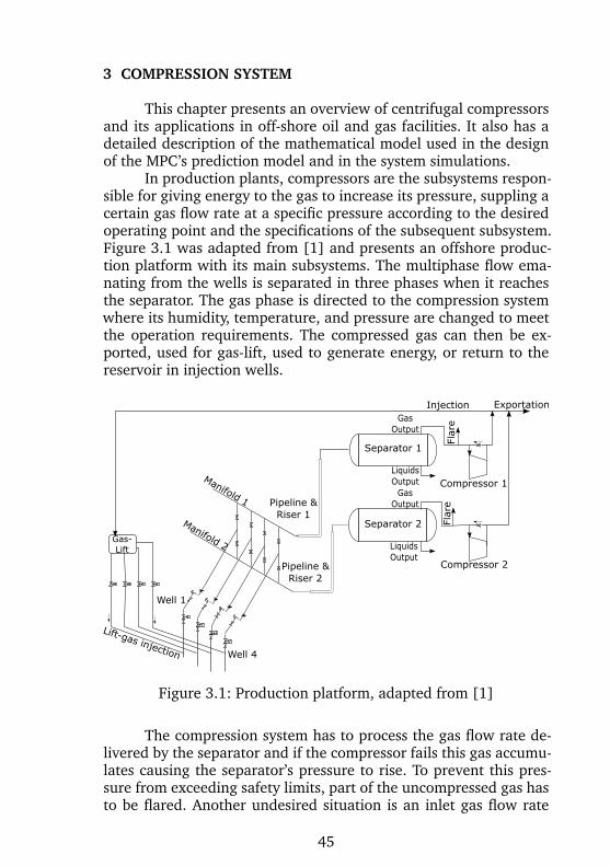
In production plants, compressors are the subsystems respon-sible for giving energy to the gas to increase its pressure, suppling acertain gas flow rate at a specific pressure according to the desiredoperating point and the specifications of the subsequent subsystem.Figure 3.1 was adapted from [1] and presents an offshore produc-tion platform with its main subsystems. The multiphase flow ema-nating from the wells is separated in three phases when it reachesthe separator. The gas phase is directed to the compression systemwhere its humidity, temperature, and pressure are changed to meetthe operation requirements. The compressed gas can then be ex-ported, used for gas-lift, used to generate energy, or return to thereservoir in injection wells.
Manifold 1
Manifold 2 Liquids
Output
Separator 1
Separator 2
Well 1
Lift-gas injection
Injection
Fla
re
Exportation
Compressor 1
Gas-
Lift
Fla
re
Compressor 2
Gas
OutputPipeline &
Riser 1
Pipeline &
Riser 2
Well 4
Gas
Output
Liquids
Output
Figure 3.1: Production platform, adapted from [1]
The compression system has to process the gas flow rate de-livered by the separator and if the compressor fails this gas accumu-lates causing the separator’s pressure to rise. To prevent this pres-sure from exceeding safety limits, part of the uncompressed gas hasto be flared. Another undesired situation is an inlet gas flow rate
45

46 Chapter 3. Compression System
below specified limits, which can take the compressor to an unsta-ble region of operation. In this case, there can be a reverse gas flowinside the compressor that causes oscillations in the pressure andflow of the gas. This phenomenon is known as compressor surge[3][4].
The centrifugal compression system of a particular platformis studied in this work. A compression stage is made of two parts:the impeller and the diffuser. The gas is sucked through the centerof the impeller and pushed by the centrifugal force to the diffuser,where the kinetic energy of the accelerated gas is then convertedto pressure. The amount of energy a gas mass unit receives fromthe compressor is called head [3]. However not all the energy isused to increase the pressure. Due to friction and other irreversiblelosses, part of the energy is lost in the form of heat. Subsection 3.3.2presents in more details the head calculation and its relation to thepressure increase.
For a compressor stage, the variables and parameters that de-fine its performance are:
\bullet ps - suction pressure
\bullet Ts - suction temperature
\bullet pd - discharge pressure
\bullet MW - molecular weight of the gas mixture
\bullet Z - gas compressibility
\bullet k - gas specific heat ratio
\bullet \eta p - polytropic efficiency
These variables and parameters define the gas flow rate thatthe compressor is able to process and the amount of power requiredto achieve it. They also define the temperature of the compressedgas, or the discharge temperature Td. Centrifugal compressors aredesigned to operate within a relatively small range of pressures,flows and gas characteristics. There are two phenomena that limitthe operation of centrifugal compressors: stonewall or choke andsurge. These phenomena, as well as the strategies to avoid them,are presented in section 3.1.
In this study the compression system consists in two parallelcompressors with three stages each. A schematic of the system is

3.1. Surge and Stonewall 47
presented in figure 3.2. The two parallel compressor trains are con-nected to the inlet header at the entrance of the system and to anexportation header at the exit.
The pressures in the system are the inlet pressure pin, the out-let pressure pout, the discharge pressures pdij , where ij refers to thecompression stage j of the compressor train i. The discharge pres-sure of one stage of compression is equal to the suction pressure ofthe next stage. The pressure ratio r is the relation between the dis-charge and the suction pressures of a certain stage and it representshow much the gas pressure has been increased. The gas mass flowrate entering and exiting the process are respectively min and mout.The mass flow rate through the compressor is m and mass flow ratethrough the recycle valve is mr.
The compression system also has PID controllers that are re-sponsible for stabilizing the suction pressure, the discharge pres-sure, and the antisurge control. This regulatory layer was also mod-eled as part of the system so the prediction models would considerthe influence of the PID controllers on the system. The MPC con-troller will not replace these PID controllers, but will work in a layerabove the regulatory system to improve the systems performance.
Figure 3.2: Compression system
3.1 SURGE AND STONEWALL
Surge is an unstable condition for the compressor operationthat results in reverse gas flow rate though the compressor and fluc-tuations in the delivered pressure and flow rate [23, 6]. The surgephenomenon is associated with high pressure ratios and gas flowrates below the nominal flow rate of the compressor and thus con-

48 Chapter 3. Compression System
stitutes the lower boundary for stable flow rates. The occurrence ofsurge can severely damage the mechanical components of the com-pressor. It is important to determine the surge point so an antisurgecontroller can avoid surge by keeping the system operating in thestable operation region. Surge control in industrial applications stillrelies on preventing the surge occurrence [5]. For every pressureratio and rotational speed there is a minimum volumetric flow rate,determined by the surge line, that guarantees the system’s stableoperation. In figure 3.3, the minimum flow is represented by pointD. A well known antisurge control strategy is to use recycle valvesto send part of the discharged compressed gas back to the suctionto increase the flow through the compressor when necessary. Sec-tion 3.4.3 explains in further details the antisurge control systeminstalled by the manufacturer in the compression system studied inthis work. The compressor manufacturer, through a series of tests,determines the operation limits of the compressor stage. The surgeand the stonewall or choke are the two phenomena that limit thecompressor’s operation and they are determined by the manufac-turer. Figure 3.3, taken from [24], illustrates the relation betweenthe volume flow rate Q and the pressure ratio r between the surgeand stonewall limits. The compressor map for a real compressordoes not define the points to the left of the surge line because thetests are not performed in the unstable region.
The stonewall phenomenon is associated with flow rates wellabove the nominal flow rate and it defines the upper boundary forstable flows. Stonewall is characterized by the occurrence of sonicspeed in the compressor’s impeller. It occurs when the system re-sistance decreases and flow increases. For a compressor of a sin-gle stage, the phenomenon happens when the head becomes null[24] and r = 1, which means the gas is flowing through the com-pressor without being compressed. The efficiency decreases due toincreased energy losses in the form of heat. Some manufacturerslimit the compressor’s operation to the choke or stonewall region,but others allow their machine to operate in the choke region aslong as the head is not negative [3].
.
3.2 SURGE INDEXES
The surge indexes are variables created to measure the dis-tance between the current operation point and the surge line. In

3.3. Modeling 49
Figure 3.3: Surge and Stonewall
[25] a surge indicator that is not affected by the gas molecularweight is proposed. But the pressure drop on the orifice plate usedto measure the volumetric gas flow has to be known and, for that,calculating this surge indicator in practice is difficult. In [13] a sim-pler surge index is presented as a performance indicator:
IS =Qsurge
Qcp(3.1)
where Qcp is the volumetric flow rate of gas through the stage andQsurge is the minimum volumetric flow that must go through thatsame stage to avoid surge at that operating point. The desired valuefor the index is IS < 1. The steps to calculate Qsurge are detailedin 3.3.1.
The IS values range from 0 to 1, where 1 means that thesystem went into surge. In this study IS is not only considered aperformance indicator but also tested as a controlled variable forthe MPC controllers discussed in chapter 4. Since the system has sixstages, three for each compression train, the complete system hassix indexes of surge, which are grouped in vector IS.
3.3 MODELING
The mathematical model of the compressor presented in thissection is based on Greitzer [7]. Greitzer model is also used in [26],[4], [27], [28], [29], [24], [30] e [31].
The equations that define the dynamics of a compression stagewere taken from [2]. The main equations are:
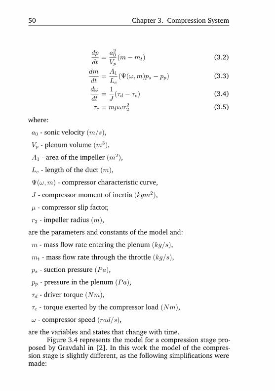
50 Chapter 3. Compression System
dp
dt=
a20Vp
(m - mt) (3.2)
dm
dt=
A1
Lc(\Psi (\omega ,m)ps - pp) (3.3)
d\omega
dt=
1
J(\tau d - \tau c) (3.4)
\tau c = m\mu \omega r22 (3.5)
where:
a0 - sonic velocity (m/s),
Vp - plenum volume (m3),
A1 - area of the impeller (m2),
Lc - length of the duct (m),
\Psi (\omega ,m) - compressor characteristic curve,
J - compressor moment of inertia (kgm2),
\mu - compressor slip factor,
r2 - impeller radius (m),
are the parameters and constants of the model and:
m - mass flow rate entering the plenum (kg/s),
mt - mass flow rate through the throttle (kg/s),
ps - suction pressure (Pa),
pp - pressure in the plenum (Pa),
\tau d - driver torque (Nm),
\tau c - torque exerted by the compressor load (Nm),
\omega - compressor speed (rad/s),
are the variables and states that change with time.Figure 3.4 represents the model for a compression stage pro-
posed by Gravdahl in [2]. In this work the model of the compres-sion stage is slightly different, as the following simplifications weremade:

3.3. Modeling 51
Figure 3.4: Compression stage configuration proposed in [2].
\bullet there is no accumulation of gas in the compressor, so in equa-tion 3.3 dm
dt = 0. This means \Psi (\omega ,m)p0 = pp. This simplifi-cation relies on the fact that the variations on m with timeinside the compressor would be very rapid and the use of thealgebraic expression assumes an instantaneous change.
\bullet it is assumed that the regulatory control system is part of themodel.
\bullet the compressor manufacturer data sheet is used to obtain therelation between discharge and suction pressure to the suctionvolumetric flow rate Q and compressor angular velocity \omega , so\Psi (\omega ,Q) = pp/ps.
\bullet there is no mass exchange between gas and liquid phase in thescrubber.
\bullet there is no energy losses in the heat exchanger. For the sakeof control algorithms development this simplification is con-sidered acceptable.
\bullet there is no change in the gas compressibility with pressure. Itis expected that Z changes would not lead to changes on theMPC algorithm choices.
The following subsections describe the equations used in thisstudy. It is important to highlight that gas flow rates, pressures, tem-peratures, valve openings, and the rotational speeds of the two com-pression trains are states or algebraic variables of the model andthey can change through time. The other elements of the model areconstants and parameters.

52 Chapter 3. Compression System
3.3.1 Compression stage
In this work, each compression stage has the main compres-sor line and a recycle line with an antisurge valve used to preventthe occurrence of surge. In the main line there is a heat exchanger, agas scrubber, and a compressor unit. The heat exchanger is respon-sible for keeping the gas temperature at the desired reference; thegas scrubber removes the gas condensate that forms because of thehigh pressure in the system; finally, the compressor unit is responsi-ble for providing energy to the gas, increasing its pressure. Figure3.5 shows the compression stage modeled in this section.
Figure 3.5: Compression stage modeled in this work
Each stage can be described by the same set of differentialequations, therefore the next subsections present the modeling ofthe inlet header, of the outlet header, and of only one stage of com-pression. Since the three stages of each compression train are con-nected in series, the discharge pressure of one stage is equal to thesuction pressure of the subsequent stage.
The original differential equations 3.2 to 3.5 do not includetemperature changes caused by the heat exchanger or the dynamicsof the recycled gas mass flow rate. So these equations were includedin the model. In the model proposed in this study, the gas accumu-lation in the plenum is not considered. Instead dp
dt is a function ofthe gas accumulation in the scrubber V (equation 3.2).
The compressor characteristic curve \Psi (\omega ,m) was obtainedfrom the compressor map provided by the manufacturer. The mapshows the relation between pressure ratio pd/ps, rotational speed \omega ,and gas flow rate mcp through each compression stage. Besides, themap also shows the surge line, which represents the minimum flow

3.3. Modeling 53
rate to avoid surge, given pd/ps and \omega . An example of compressionmap is given in figure 3.8.
After the modifications and the addition of the heat exchangerand recycle loop dynamics, the set of equations 3.2 to 3.5 waschanged. The new set of equations that represents a compressionstage is:
dpsdt
=ZRTs
MWVs(mhe - mcp) (3.6)
d\omega
dt=
1
J(\tau d - \tau c) (3.7)
\tau c = \omega mcp\mu r22 (3.8)
mhe = mr +msin (3.9)
where:
Z - gas compressibility factor
MW - gas molecular weight (kg/mol)
R - gas constant (J/mol)
ps - suction pressure of the stage (Pa)
Ts - suction temperature of the stage (K)
Vs - volume of the scrubber (m3)
mhe - gas mass flow rate through the heat exchanger (kg/s)
mcp - gas mass flow rate through the compressor unit (kg/s)
mr - gas mass flow rate through the recycling line (kg/s)
msin - gas mass flow rate that enters the stage (kg/s)
The discharge pressure of stage i is equal to the suction pres-sure of the subsequent stage i + 1, so pd,i = ps,i+1, and ps is deter-mined by solving the differential equation 3.6 for each stage. Thepressure ratio for each stage is ri = pd,i/ps,i. From equation 3.3,considering dm
dt = 0, the pressure ratio is related to \omega and mcp by:
\Psi (\omega ,mcp) =pdps
(3.10)

54 Chapter 3. Compression System
In a compression stage, the relation between r, \omega , and thevolumetric flow rate Qcp is given by the manufacture’s compressionmap and can be approximated through a polynomial:
r = a+ bx - cy - dx2 + exy + fy2 (3.11)
with:
r =pdps
y =\omega
\omega nom
x =Qcp
y
where \omega nom is the compressor nominal rotational speed. Since, rand y are known, x is the one of the roots of 3.11. Figure 3.6 showsthe relation between the volumetric flow rate and the pressure ratiofor a few normalized rotational speeds. The surge line shown in thefigure is where the pressure ratio is maximum and dr/dQ = 0. Thesurge volumetric flow Qsurge is Q at the point where dr/dQ = 0.
dr
dQ=
dr
dx
dx
dQ
dr
dQ= b
dx
dQ+ 2dx
dx
dQ+ ey
dx
dQ(3.12)
Replacing x = Qsurge/y, y = \omega /\omega nom, and dx/dQ = 1/y inequation 3.12:
dr
dQ=
b
y+
2d
yx+ e = 0
2d
y2Qsurge = - b
y - e
Qsurge = - (by + ey2)
2d
Qsurge = - b\omega
2d\omega nom+
- e\omega 2
2d\omega 2nom
To simplify the calculations, Qsurge can be written as a func-tions of \omega :

3.3. Modeling 55
Qsurge = k1\omega + k2\omega 2
k1 = - b
2d\omega nom
k2 = - e
2d\omega 2nom
The manufacture’s compression map does not show the sys-tem’s behavior for the region where dr/dQ < 0, the part of the curveto the left of the surge line, because this is the unstable operationregion and the system is not tested in these operation conditions.The compressor’s stable operation region is to the right of the surgeline. So x is the root of polynomial 3.11 that is to the right of thepoint where dr/dQ = 0.
Figure 3.6: Relation between volumetric flow rate, pressure ratio,and normalized rotational speed
The gas volumetric flow rate Qcp through the compressor iscalculated from x, Qcp = xy. The gas mass flow rate through acompressor stage mcp depends of the gas density \rho :
mcp = \rho Qcp (3.13)
\rho =MW
ZRTsps (3.14)
The recycled gas mass flow rate is computed using the equa-tions for valves working with compressible fluids as recommended

56 Chapter 3. Compression System
by [32]:
mr = NunCV Y pd
\sqrt{} \biggl( MWx
ZRTd
\biggr) (3.15)
CV = CVN\Phi r (3.16)
Fk =k
1.4(3.17)
x = min
\biggl( pd - ps
pd, FkxT
\biggr) (3.18)
Y = 1 - x
3FkxT(3.19)
where:
mr - gas mass flow rate through the recycling line (kg/s)
Nun - constant that converts the units
CVN - flow coefficient
k - heat capacity ratio
The discharge temperature of the compressed gas can be ob-tained as:
Td = Ts
\biggl( pdps
\biggr) k - 1\eta pk
. (3.20)
where:
\eta p - polytropic efficiency
3.3.2 Power consumption
The head H is the amount of work per mass unit that has tobe applied to the gas to compress it. According to [24], the energybalance in the compression can be expressed as:
H + dq = dh+c2
2+ gdz (3.21)
where dq is the heat exchanged inside the impeller, dh is the varia-tion of the gas enthalpy, c2
2 is the kinetic energy of the gas, and gdzis the gravitational energy of the gas.

3.3. Modeling 57
The process is considered to be adiabatic, so there is no heatexchange and dq = 0. The kinetic and gravitational energies are toosmall and can also be disregarded. So the head can be consideredthe energy required to change the enthalpy of the gas and it is givenby:
H = dh (3.22)
The enthalpy variation is:
dh =dp
\rho (3.23)
where p is the gas pressure and \rho is the gas density.Thus, the work per mass unit required to compress a gas from
pressure p1 to pressure p2 can be obtained by:
H =
\int p2
p1
dp
\rho (3.24)
The gas density \rho can be expressed differently if the compres-sion is isentropic, isothermal, or polytropic. The isentropic compres-sion is adiabatic and reversible and the entropy is constant. Theisothermal is also reversible and in this case the temperature re-mains constant. The polytropic compression is adiabatic but irre-versible and in this case the efficiency of the compression is con-stant.
The polytropic compression is considered more appropriateaccording to [3]. In that case,
p
\rho n= cte (3.25)
\rho = \rho 1
\biggl( p
p1
\biggr) 1/n
(3.26)
n is the polytropic exponent. Replacing equation 3.26 in 3.24:
H =p1/n1
\rho 1
\int p2
p1
dp
p1/n(3.27)
After solving the integral in equation 3.27, the head equationbecomes:
H =p1/n1
\rho 1
\Biggl( p
- 1n +1
- 1n + 1
\Biggr) \bigm| \bigm| \bigm| \bigm| \bigm| p2
p=p1

58 Chapter 3. Compression System
with
\rho 1 =p1MW
Z1RT1(3.28)
where MW is the gas molecular weight, Z1 is the gas compressibil-ity at point 1, and T1 is the gas temperature at point 1. Replacingequation 3.28 in 3.3.2 gives:
H =Z1RT1
MW
n
n - 1
\Biggl[ \biggl( p2p1
\biggr) n - 1n
- 1
\Biggr] . (3.29)
The polytropic exponent n can be expressed in therms of the poly-tropic efficiency \eta p and the gas specific heat ratio k:
n - 1
n\approx k - 1
\eta pk(3.30)
The polytropic efficiency \eta p is also calculated from a polyno-mial obtained from the compressor’s manufacturers data sheet.
Thus, the equation for the head becomes:
H =Z1RT1
MW
\eta pk
k - 1
\Biggl[ \biggl( p2p1
\biggr) k - 1\eta pk
- 1
\Biggr] . (3.31)
The absorbed compressor power P is given by:
P =mcpH
\eta p(3.32)
where mcp is the gas mass flow rate going through the compressor.
3.3.3 Inlet header
The inlet header is represented by a compressor inlet drumwith volume Vin, shown in figure 3.7.
The gas phase from the separator reaches the compressionsystem with a mass flow rate min. From the inlet header, the gasmass flow rate is divided between the two compression trains. Con-nected to this vessel is also the flare line with a flare valve. Thisvalve opens releasing gas to the flare if the pressure in the inletheader pin reaches its maximum limit. The pressure pin depends on

3.3. Modeling 59
Figure 3.7: Inlet header
the mass balance in the vessel.
dpindt
=RZTin
MWVin(min - min,1 - min,2 - mflare) (3.33)
min,1 = k1he
\sqrt{} MW
ZRTin
\sqrt{} pin(pin - p1s) (3.34)
min,2 = k2he
\sqrt{} MW
ZRTin
\sqrt{} pin(pin - p2s) (3.35)
where:
pin - pressure in the inlet header
Vin - volume of the compressor inlet drum
Tin - temperature of the gas entering the compression system
min - gas mass flow rate entering the compression system
min,1 - gas mass flow rate entering the compression train 1
min,2 - gas mass flow rate entering the compression train 2
mflare - gas mass flow rate in the flare line
ps,1 - suction pressure of stage 1 of compression train 1
60 Chapter 3. Compression System
ps,2 - suction pressure of stage 1 of compression train 2
In equations 3.34 and 3.35, khe,1 and khe,2 are constants thatrepresent the pressure drop in the heat exchanges 1 e 2.
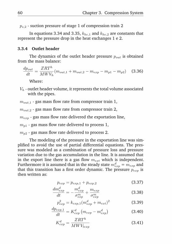
3.3.4 Outlet header
The dynamics of the outlet header pressure pout is obtainedfrom the mass balance:
dpoutdt
=ZRTh
MWVh(mout,1 +mout,2 - mexp - mp1 - mp2) (3.36)
Where:
Vh - outlet header volume, it represents the total volume associatedwith the pipes.
mout,1 - gas mass flow rate from compressor train 1,
mout,2 - gas mass flow rate from compressor train 2,
mexp - gas mass flow rate delivered the exportation line,
mp1 - gas mass flow rate delivered to process 1,
mp2 - gas mass flow rate delivered to process 2.
The modeling of the pressure in the exportation line was sim-plified to avoid the use of partial differential equations. The pres-sure was modeled as a combination of pressure loss and pressurevariation due to the gas accumulation in the line. It is assumed thatin the export line there is a gas flow mext which is independent.Furthermore it is assumed that in the steady state md
exp = mexp andthat this transition has a first order dynamic. The pressure pexp isthen written as:
pexp = pexp,1 + pexp,2 (3.37)
dmdexp
dt= -
mdexp
\sigma mexp
+mexp
\sigma mexp
(3.38)
p2exp = kexp,1(mdexp +mext)
2 (3.39)dpexp,1
dt= Kd
exp
\bigl( mexp - md
exp
\bigr) (3.40)
Kdexp =
ZRTh
MWVlexp(3.41)

3.4. Regulatory control 61
where:
\sigma mexp - time constant,
kexp,1 - constant that depends on the length and diameter of the ex-port line, the friction factor, and the average pressure throughthe line,
Vlexp - volume of the exportation line.
3.4 REGULATORY CONTROL
The regulatory control system is formed by PID controllersand it was also modeled as part of the compression system. EveryPID has an anti-windup. The regulatory control system consideredin the compressor modeling presented in this dissertation is com-posed by:
1. Inlet gas pressure and load sharing control
2. Outlet gas pressure and exportation flow control
3. Antisurge control
4. Suction temperature control
3.4.1 Inlet pressure and load sharing
The compressor inlet pressure pin depends on the mass bal-ance of the vessel Vin, shown in equation 3.33.
The manipulation of min,1 and min,2 can take pin to the de-sired value. The flows min,1 and min,2 depend on the rotationalspeed of the compressor w, which depends on the power P applied

62 Chapter 3. Compression System
to the compressor. The control law for pin is given by:
epin = - pspin + pin (3.42)
upin,1 = Kppinepin +Kipin
\int t
0
epin(\tau )d\tau + ubias,1 (3.43)
upin,2 = Kppinepin +Kipin
\int t
0
epin(\tau )d\tau + ubias,2 (3.44)
ubias,1 = Kpbiasedsm,1 +Kibias
\int t
0
edsm,1(\tau )d\tau (3.45)
ubias,2 = Kpbiasedsm,2 +Kibias
\int t
0
edsm,2(\tau )d\tau (3.46)
edsm,1 = dmeansurge - dsurge,1 (3.47)
edsm,2 = dmeansurge - dsurge,2 (3.48)
dsurge,1 = Q1 - Qsurge,1 (3.49)dsurge,2 = Q2 - Qsurge,2 (3.50)
dmeansurge =
dsurge,1 + dsurge,22
(3.51)
where:
epin - error between the setpoint and pin,
pspin - setpoint for pin,
Kppin - proportional gain of the inlet pressure controller,
Kipin - integral gain of the inlet pressure controller
Kpbias - proportional gain of the load sharing controller,
Kibias - integral gain of the load sharing controller
Q1 and Q2 - volumetric flow rate through the first stage of com-pressor train 1 and 2, respectively
Qsurge,1 and Qsurge,2 - surge volumetric flow rate for the first stageof compressor train 1 and 2, respectively
The terms ubias,1 and ubias,2 implement the load sharing, sothat both compressor trains are always at the same distance of thesurge point.
3.4. Regulatory control 63
3.4.2 Outlet header pressure
The outlet header pressure pout depends on the mass balancemout,1 + mout,2 - mexp - mp1 - mp2, as shown in equation 3.36.The gas flow rate directed to the exportation line mexp is regulatedby the exportation valve opening \phi exp. The pressure pout can bechanged by manipulating \phi exp. The control law for \phi exp is given by:
epout = pspout - pout (3.52)
\phi exp = - Kcexp \ast epout - Kiexp
\int t
0
epout(\tau )d\tau
where:
epout - error between the setpoint and pout,
pspout - setpoint for pout,
Kpexp - proportional gain of the outlet pressure controller,
Kiexp - integral gain of the outlet pressure controller
3.4.3 Antisurge control
Compressor data sheets are usually provided by the compres-sor manufacturer. They contain important information on the com-pressor’s behavior and operating points. Figure 3.8 shows a typicalcompressor map taken from a compressor’s data sheet. The graphshows the relation between the volumetric flow rate at compressor’ssuction and the pressure ratio for different rotational speeds. In themap, the red solid line is known as the surge line. As explainedin section 3.1, this line defines the minimum flow required to avoidsurge, Qsurge. Anti surge control techniques usually consider a safersurge line, called control surge line or safe surge line, representedby the blue dashed line on the graph. Commonly, the control surgeline is the surge line plus a slack of 5 - 10\% of the minimum flowrate.
If the compressor is working at a point to the left of the safesurge line then the flow rate through the compressor is below theminimum. Recycling part of the compressed gas can increase thegas flow through the compressor, preventing the system to go intosurge. And if the compressor is working at a point to the right ofthe safe surge line, no action is required.

64 Chapter 3. Compression System
Surge line
Control line
Figure 3.8: Example of a compressor map
So the antisurge control of this system consists on opening arecycle valve allowing part of the discharged compressed gas to goback to compressor suction. This will increase the compressor’s gasflow keeping it above the minimum and avoiding surge.
The minimum flow obtained through the control surge lineQsurge is used to define the setpoint for the PI controller Qsp
surge asshown in equation 3.53.
Qspsurge = Qsurge(1 + slack) (3.53)
For each stage there is an antisurge recycling valve. The valveopening, \phi r is determined by the control law in equation 3.55.
es = Qspsurge - Q (3.54)
\Phi r = Kpres +Kir
\int t
0
es(\tau )d\tau (3.55)
where:
Q - flow through the compressor stage,

3.4. Regulatory control 65
Kpr - proportional gain of the PI controller,
Kir - integral gain of the PI controller,
3.4.4 Suction temperature control
On the suction of each compression stage there is a heat ex-changer that keeps the suction temperature at a desired value. Thegas temperature control is based on the coolant flow.
Figure 3.9: Gas flows through the heat exchanger
Figure 3.9 shows the important flows used in the modeling ofthe temperature control where:
mE - gas mass flow from inlet header or from the previous stage,
mr - recycled gas mass flow,
mhe - gas mass flow trough the heat exchanger,
mc - coolant mas flow,
The amount of energy in the heat exchanger is given by Win:
Win = mrcgTd +mEcgTE +\Phi hemmaxc ccTc. (3.56)
where:
TE - inlet gas temperature,
Td - discharge gas temperature (same as the temperature of therecycled gas),
Ts - suction gas temperature,
Tc - coolant temperature,
cg - gas specific heat,

66 Chapter 3. Compression System
cc - coolant specific heat,
\Phi he - heat exchanger valve opening.
In steady state the coolant and the gas temperatures are con-sidered the same since the modeling assumes no heat losses:
Wout = (mhecg +\Phi hemmaxc cc)T
sss (3.57)
Considering no energy loss, Win = Wout and
T sss = (mRcgTd +mEcgTE +\Phi hem
maxc ccTC) /(mTCcg+\Phi hem
maxc cC).
(3.58)Assuming a first order dynamics, the suction temperature’s
differential equation Ts is:
dTs
dt= - Ts
\sigma Ts+
T sss
\sigma Ts(3.59)
The heat exchanger’s valve opening \Phi he is given the controllaw in equation 3.61:
eTs = T sps - Ts (3.60)
\Phi he = KpTseTs +KiTs
\int t
0
eTs(\tau )d\tau (3.61)
3.5 SYSTEM SIMULATION
This section analyses the system’s behavior without the MPClayer. Here only the regulatory control is active. This results will bethe base for comparison of the proposed MPC controllers in the nextchapters. The two compressor trains are identical so only the resultsof one the trains are shown in this section.
The compression system nonlinear model described in section3.3 was implemented in Matlab and the differential equations weresolved with ODE45. For the simulations and comparisons a simplescenario was chosen, where the inlet flow varies as illustrated infigure 3.10. This input flow is the main disturbance applied to thesystem to create the scenario. The simulation starts with the flowon its nominal value. Then the flow drops by 50\%. This drives thesystem to the surge region. After the drop, the inflow rises to 115\%of its nominal value, forcing the system to flare gas. The results ofthe regulatory controlled system are shown in figures 3.11 to 3.17.

3.5. System simulation 67
0 5 10 15 20 25 30 35Time [min]
10
15
20
25m
in [
kg/s
]
Figure 3.10: Inlet gas flow
Figure 3.11 shows that the inlet pressure controller is able tokeep pin at its setpoint pspin = 6.2 when min is low, but when min ishigher than the compressor’s capacity, the rotational speed reachesits maximum limit and pin increases. When pin reaches the reliefvalve pressure limit, the flare valve opens and allowing gas to flowto the flaring system, as can be seen in figure 3.12.
0 5 10 15 20 25 30 35Time [min]
6
6.5
7
p in [
bar]
Figure 3.11: Results of the regulatory control system - inlet headerpressure
Figures 3.13 to 3.15 show the surge indexes and the antisurgevalves openings. As min decreases the surge indexes increase. When
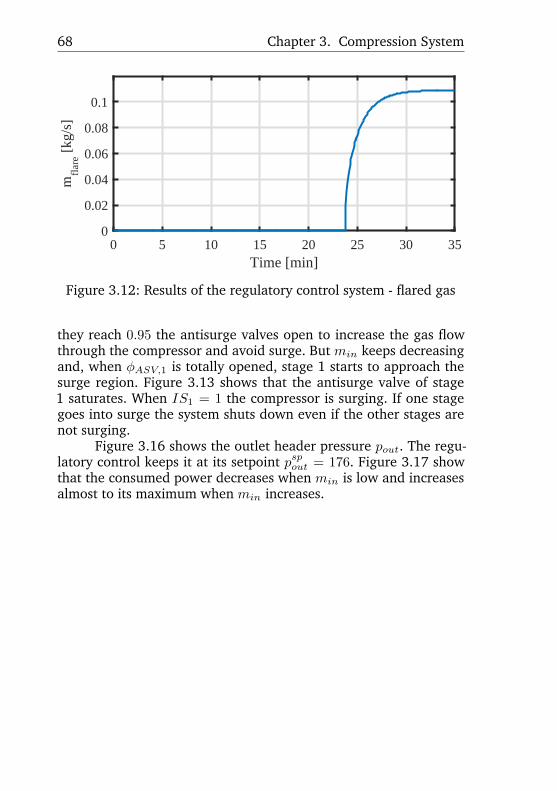
68 Chapter 3. Compression System
0 5 10 15 20 25 30 35Time [min]
0
0.02
0.04
0.06
0.08
0.1
mfl
are [
kg/s
]
Figure 3.12: Results of the regulatory control system - flared gas
they reach 0.95 the antisurge valves open to increase the gas flowthrough the compressor and avoid surge. But min keeps decreasingand, when \phi ASV,1 is totally opened, stage 1 starts to approach thesurge region. Figure 3.13 shows that the antisurge valve of stage1 saturates. When IS1 = 1 the compressor is surging. If one stagegoes into surge the system shuts down even if the other stages arenot surging.
Figure 3.16 shows the outlet header pressure pout. The regu-latory control keeps it at its setpoint pspout = 176. Figure 3.17 showthat the consumed power decreases when min is low and increasesalmost to its maximum when min increases.

3.5. System simulation 69
0 5 10 15 20 25 30 35Time [min]
0.7
0.8
0.9
1
IS1 [
-]
(a) Surge index
0 5 10 15 20 25 30 35Time [min]
0
0.2
0.4
0.6
0.8
1
ΦA
SV1
[-]
(b) Antisurge valve opening
Figure 3.13: Results of the regulatory control system - Stage 1

70 Chapter 3. Compression System
0 5 10 15 20 25 30 35Time [min]
0.6
0.7
0.8
0.9
1
IS2 [
-]
(a) Surge index
0 5 10 15 20 25 30 35Time [min]
0
0.2
0.4
0.6
0.8
ΦA
SV2
[-]
(b) Antisurge valve opening
Figure 3.14: Results of the regulatory control system - Stage 2

3.5. System simulation 71
0 5 10 15 20 25 30 35Time [min]
0.5
0.6
0.7
0.8
0.9
1
IS3 [
-]
(a) Surge index
0 5 10 15 20 25 30 35Time [min]
0
0.2
0.4
0.6
0.8
ΦA
SV3
[-]
(b) Antisurge valve opening
Figure 3.15: Results of the regulatory control system - Stage 3

72 Chapter 3. Compression System
0 5 10 15 20 25 30 35Time [min]
175.8
175.9
176
176.1p ou
t [ba
r]
Figure 3.16: Results of the regulatory control system - outlet headerpressure
0 5 10 15 20 25 30 35Time [min]
0.6
0.7
0.8
0.9
1
Nom
aliz
ed p
ower
[-]
Figure 3.17: Power consumption
The simulated scenario shows that for a gas inflow drop of50\% this system would go into surge. A real compression systemwould stop working if it went into surge. So, the system’s behaviorobserved when IS = 1 is not real. However, this simulation showsthat, for this min disturbance, the regulatory control was not ableto avoid surge. Based on that, an advanced control algorithm couldbe implemented to improve the compression system’s performance.

3.6. Control objectives 73
3.6 CONTROL OBJECTIVES
The MPC designed for the compression system has these con-trol objectives:
\bullet To avoid surge and system’s shutdown increasing the MeanTime Between Failure (MTBF) of the compressor system
\bullet To minimize gas flaring
\bullet To minimize energy consumption
The setpoints for the regulatory control could be used as ma-nipulated variables for the MPC controller. The antisurge PID con-troller allows another signal to override its output, sending a differ-ent signal to the antisurge valve. So the antisurge valve openingscould also be manipulated variables.
To avoid the occurrence of surge, the surge indexes could beused as controlled variables. The compressors energy consumptionE could be expressed as a component of the control objective func-tion J . The compressors energy consumption can be expressed asthe sum of the integral of the power along the prediction horizonfor each compressor.
E =2\sum
j=1
Ej (3.62)
Ej =
\int to+N
to
Pj(t)dt (3.63)
Besides these objectives, the suction and discharge pressuresof each stage have to be kept within their operation limits. Theycould also be included as controlled variables or as constraints forthe optimization problem that calculates the control increments.
3.7 LINEAR MODEL
The nonlinear model of the compression system, includingthe regulatory control, is given by a set of algebraic and differentialequations. The outputs y of the system are a function of the statesx and the control signals u. This relation is represented by equation3.64.

74 Chapter 3. Compression System
y = f(x, u) (3.64)
In [33] the Practical Non Linear MPC (PNMPC) is introduced.In this work the author shows that the matrix G used by the MPCmay be obtained from the Jacobian matrix of the system:
G =
\biggl[ \partial f
\partial u
\biggr] =
\left[ \partial f(t+1| t)
\partial u(t) 0 . . . 0\partial f(t+2| t)
\partial u(t)\partial f(t+2| t)\partial u(t+1) . . . 0
......
. . ....
\partial f(t+N | t)\partial u(t)
\partial f(t+N | t)\partial u(t+1) . . . \partial f(t+N | t)
\partial u(t+N - 1)
\right] (3.65)
If the system is considered to be time-invariant, then G canbe approximated to:
G =
\biggl[ \partial f
\partial u
\biggr] =
\left[ \partial f(t+1| t)
\partial u(t) 0 . . . 0\partial f(t+2| t)
\partial u(t)\partial f(t+1| t)
\partial u(t) . . . 0...
.... . .
...\partial f(t+N | t)
\partial u(t)\partial f(t+N - 1| t)
\partial u(t) . . . \partial f(t+1| t)\partial u(t)
\right] (3.66)
Thus, for a linear system as well as for a linearized repre-sentation [34], the matrix G is equivalent to the one built in theDMC controller algorithm. The first column of the matrix G is thestep response of the system and it is also used to calculate the freeresponse. The vector with the step response coefficients g can beobtained by:
g =f(\=x, \=u+\Delta u) - f(\=x, \=u)
\Delta u(3.67)
where (\=x, \=u) is the point where the function is linearized. In thisstudy, the system was linearized off-line at an equilibrium point thatcorresponds to the system’s steady state xss and uss. So, \=x = xss and\=u = uss. The same linearized models were used through the entiresimulations.
3.7.1 Step responses analysis
Instead of the coefficients of the step responses normally usedin linear MPC control systems, the coefficients obtained using the
3.7. Linear model 75
PNMPC technique were used here. For a linear system these coef-ficients would be identical to the ones obtained with the applica-tion of a step [33]. However for a nonlinear system the PNMPCcoefficients correspond to the coefficients of the linearized system.For simplicity, these coefficients will be called step responses. Thissubsection presents the analysis of these linear models so the mostadequate variables can be selected to be used by the MPC controller.
Considering the setpoints and manipulations that can be changedin the compression system regulatory system, the possible manipu-lated variables are:
\bullet u1 - setpoint of the inlet gas pressure (pspin)
\bullet u2 - setpoint of the outlet gas pressure (pspout)
\bullet u3 - opening of the antisurge valve of stage 11 (\phi ASV,11)
\bullet u4 - opening of the antisurge valve of stage 12 (\phi ASV,12)
\bullet u5 - opening of the antisurge valve of stage 13 (\phi ASV,13)
\bullet u6 - opening of the antisurge valve of stage 21 (\phi ASV,21)
\bullet u7 - opening of the antisurge valve of stage 22 (\phi ASV,22)
\bullet u8 - opening of the antisurge valve of stage 23 (\phi ASV,23)
Based on the control objectives described in section 3.6, thepossible controlled variables are:
\bullet y1 - discharge pressure of stage 11 (pd11)
\bullet y2 - discharge pressure of stage 12 (pd12)
\bullet y3 - discharge pressure of stage 21 (pd21)
\bullet y4 - discharge pressure of stage 22 (pd22)
\bullet y5 - surge index of stage 11 (IS11)
\bullet y6 - surge index of stage 12 (IS12)
\bullet y7 - surge index of stage 13 (IS13)
\bullet y8 - surge index of stage 21 (IS21)
\bullet y9 - surge index of stage 22 (IS22)

76 Chapter 3. Compression System
\bullet y10 - surge index of stage 23 (IS23)
\bullet y11 - consumed power (P )
The step responses coefficients were normalized by:
srnormnm = srnmrangemuynnom
\times 100\% (3.68)
where srnm is the vector with the step response coefficients betweenthe controlled variable n and the manipulated variable m, rangemuis the range of the manipulated variable m, and ynnom is the nominalvalue of the controlled variable n. Thus, srnormnm shows the percent-age variation of n in relation to its nominal value, for a variation inm.
Figures 3.18 to 3.21 show the step responses between the pos-sible manipulated variables u and the possible controlled variablesy. The coefficients of the step responses were normalized by equa-tion 3.68. The inter stage discharge pressures pd (y1 to y4), shownin figure 3.18, are highly sensitive to changes in u1 and u2. But y1and y3 are linearly dependent of y2 and y4 respectively. Besides,if u1 and u2 are kept within their limits, y1 to y4 also stay withintheir limits. So instead of using them as controlled variables, theirlower and upper limits were included in the problem’s constraintsto be safe. The indexes of surge IS (y5 to y10), shown in figures3.19 and 3.20, are highly influenced by changes in the antisurgevalve openings (u3 to u8). The consumed power P (y11), shown infigure 3.21, is influenced by all the manipulated variables. The gainbetween u1 and P is negative while the gain between the rest of themanipulated variables and P is positive. These results suggest that,at this operating point, P could be minimized if u1 is maximizedwhile u2 to u8 are minimized.
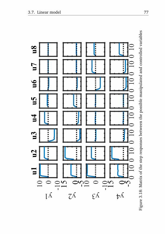
3.7. Linear model 77
-100
10
y1u1
u2
u3
u4
u5
u6
u7
u8
y2
-100
10
y3 y4
010010010010010010010010
15 0 -5 15 0 -5
Figu
re3.
18:M
atri
xof
the
step
resp
onse
sbe
twee
nth
epo
ssib
lem
anip
ulat
edan
dco
ntro
lled
vari
able
s

78 Chapter 3. Compression System
u1
u2
u3
u4
u5
u6
u7
u8
-10 0 10
y5
-10 0 10
y6y7
010010010010010010010010
300
-10
Figure3.19:M
atrixofthe
stepresponses
between
thepossible
manipulated
andcontrolled
variables
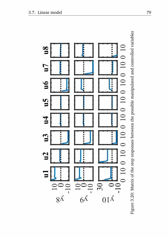
3.7. Linear model 79
u1
u2
u3
u4
u5
u6
u7
u8
-10010
y8
-10010
y9 y10
010010010010010010010010
30 0
-10
Figu
re3.
20:M
atri
xof
the
step
resp
onse
sbe
twee
nth
epo
ssib
lem
anip
ulat
edan
dco
ntro
lled
vari
able
s

80 Chapter 3. Compression System
u1
u2
u3
u4
u5
u6
u7
u8
010
y11
010010010010010010010
50
-15
Figure3.21:M
atrixofthe
stepresponses
between
thepossible
manipulated
andcontrolled
variables

3.7. Linear model 81
The relation between P and pin is particularly interesting.There is a direct relation between the gas mass flow rate mcp andconsumed power P , meaning that an increase on mcp implies in thegreater consumption of power. At the same time there is a directrelation between the head H and P . Since the head depends onthe pressure ratio r = pd/ps and assuming a fixed discharge pres-sure pd, it is possible to conclude that there is an inverse relationbetween the suction pressure ps and the consumed power P . Thatis, if the suction pressure is increased, less power is required in thecompression process.
P =mcpH
\eta p(3.69)
H =Z1RT1
MW
\eta pk
k - 1
\Biggl[ \biggl( pdps
\biggr) k - 1\eta pk
- 1
\Biggr] . (3.70)
When the compressor is not recycling, the static gain betweenps and P is negative. In this situation, changes in the pressure willnot result in changes in the gas mass flow through the compressor.But when the compressor is recycling gas to avoid surge, a reductionin ps moves the system away from the surge region, which leads toa reduction on the recycled gas flow mr and consequently on theflow through the compressor mcp. As explained before, a reductionin mcp leads to a reduction in power consumption. So, if there isgas recirculation, the static gain between ps and P could becomepositive.
Figure 3.22 shows the static relation between pin, P , and\phi 1ASV . These values were obtained for a low gas flow rate, when
the compression system is forced to recycle gas to avoid surge. Thedashed blue line represents the relation between pin and the anti-surge valve opening of the first stage \phi 1
ASV in steady state. In thissituation, smaller values of pin require smaller \phi 1
ASV to avoid surge.The solid red line represents the relation between pin and the con-sumed power P . In this situation the gain between these variableschanges signal. For this reason, including the model for pin \times P inthe prediction model of the MPC could decrease the system’s perfor-mance instead of improving it.

82 Chapter 3. Compression System
φASV
P
Norm
iliz
ed p
ow
er [
-]
0.652
0.650
0.648
0.646
φA
SV
[-]
0.6
0.5
0.4
0.3
pin
[bar]4.4 4.6 4.8 5.0 5.2 5.4 5.6 5.8 6.0 6.2
Figure 3.22: Static relation between pin, P , and \phi ASV,1
3.7.2 Variables selection
Considering the step responses analysis presented in 3.7.1,and which setpoints and valve openings can be changed in the com-pression system regulatory system, the possible manipulated vari-ables are:
\bullet pspin - setpoint of the inlet gas pressure
\bullet pspout - setpoint of the outlet gas pressure
\bullet \phi ASV,11 - opening of the antisurge valve of stage 11
\bullet \phi ASV,12 - opening of the antisurge valve of stage 12
\bullet \phi ASV,13 - opening of the antisurge valve of stage 13
\bullet \phi ASV,21 - opening of the antisurge valve of stage 21
\bullet \phi ASV,22 - opening of the antisurge valve of stage 22
\bullet \phi ASV,23 - opening of the antisurge valve of stage 23
Based on the control objectives described in section 3.6, thepossible controlled variables are:
\bullet IS11 - surge index of stage 11

3.8. Final comments 83
\bullet IS12 - surge index of stage 12
\bullet IS13 - surge index of stage 13
\bullet IS21 - surge index of stage 21
\bullet IS22 - surge index of stage 22
\bullet IS23 - surge index of stage 23
Besides these variables, the energy consumption E could beincluded as an additional objective in the objective function to guar-antee energy minimization.
The energy consumption depends on the power consumedby the compression system. As explained before, the static gain be-tween pin and P changes with the operation point. Changes in thesignal of static gains can be difficult for the linear MPC algorithm tocorrect and the controller could not work properly.
3.8 FINAL COMMENTS
This chapter described the compression system studied in thisdissertation, with a detailed description of the system’s mathemat-ical model. This nonlinear model was used to simulate the systemand to study its behavior. This model, that is one of the contribu-tions of this work, was published in [25, 35].
This chapter also presented an analysis of the potential con-trolled and manipulated variables to be used by the MPC controllersto achieve the control objectives. Based on the variables selection,the linearized prediction models were then obtained from the non-linear model.
Next chapter presents two MPC controllers. In the first one,the manipulated variables are driven to values that minimize thepower consumption. The total energy is then minimized indirectly.In the second formulation, the energy consumption is minimizeddirectly in the objective function. This requires a linear model to ex-press the dynamics between the manipulated variables and energyconsumption

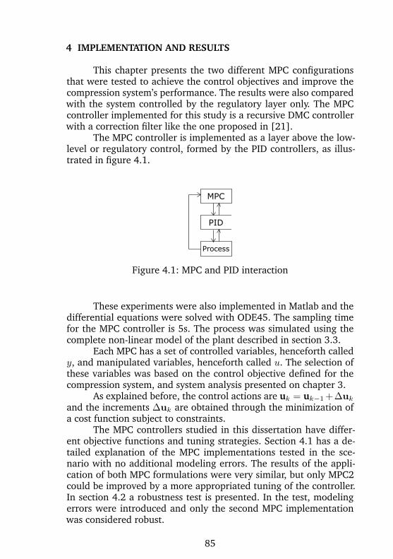
4 IMPLEMENTATION AND RESULTS
This chapter presents the two different MPC configurationsthat were tested to achieve the control objectives and improve thecompression system’s performance. The results were also comparedwith the system controlled by the regulatory layer only. The MPCcontroller implemented for this study is a recursive DMC controllerwith a correction filter like the one proposed in [21].
The MPC controller is implemented as a layer above the low-level or regulatory control, formed by the PID controllers, as illus-trated in figure 4.1.
MPC
PID
Process
Figure 4.1: MPC and PID interaction
These experiments were also implemented in Matlab and thedifferential equations were solved with ODE45. The sampling timefor the MPC controller is 5s. The process was simulated using thecomplete non-linear model of the plant described in section 3.3.
Each MPC has a set of controlled variables, henceforth calledy, and manipulated variables, henceforth called u. The selection ofthese variables was based on the control objective defined for thecompression system, and system analysis presented on chapter 3.
As explained before, the control actions are uk = uk - 1+\Delta \bfu k
and the increments \Delta \bfu k are obtained through the minimization ofa cost function subject to constraints.
The MPC controllers studied in this dissertation have differ-ent objective functions and tuning strategies. Section 4.1 has a de-tailed explanation of the MPC implementations tested in the sce-nario with no additional modeling errors. The results of the appli-cation of both MPC formulations were very similar, but only MPC2could be improved by a more appropriated tuning of the controller.In section 4.2 a robustness test is presented. In the test, modelingerrors were introduced and only the second MPC implementationwas considered robust.
85

86 Chapter 4. Implementation and Results
4.1 MPC IMPLEMENTATIONS
The MPC controllers exposed in this section are variations ofthe DMC algorithm, as explained in section 2.2. The first MPC imple-mented (section 4.1.1) does not consider the energy consumptiondirectly in its formulation due to its very nonlinear relation withthe manipulated variables. The energy consumption was includedin the second MPC formulation (section 4.1.2). As this process hasvariables with very different dynamics and amplitudes, tuning theMPC is not straightforward. Hence, in section 4.1.3 the satisficingtuning technique was applied to the MPC2 formulation to obtainmore appropriate weights. The application of the technique led to aimproved controller performance. The results were also comparedagainst the system controlled only with the PID controllers. Thiscomparison is carried out in the same scenario explained in sec-tion 3, where the gas flow rate that enters the compression systemwas used to disturb the plant’s behavior. Figure 4.2 represents thechanges in the gas flow rate min during the simulation. The flowstarts at 21.5857 kg/s, then it drops to 50% of the initial value,causing the system to go into surge without a proper control strat-egy. After that the flow rises to 115% of its initial value, causing theinput pressure to go above its maximum limit, that can cause theflare of part of the entering gas.
0 5 10 15 20 25 30 35
Time [min]
10
15
20
25
kg/
s
Figure 4.2: Gas flow rate that enters the compression system - min
The controlled and manipulated variables, the objective func-tion, and the constraints were chosen based on the compressionsystem analysis presented in chapter 3 and are described for eachcontroller in the following sections.

4.1. MPC implementations 87
4.1.1 MPC 1
The energy consumption can be minimized if pin is maxi-mized and pout and mr are minimized. For this compression sys-tem it is easy to determine the ideal values for the manipulatedvariables that guarantee energy saving. So, instead of consideringthe consumed energy as a term in the control objective function,this first MPC was designed to drive the manipulated variables totheir ideal values whenever possible. With this formulation, it is notnecessary to include the model that relates the power with the ma-nipulated variables, so the controller will not have to deal with itsnonlinearities.
Controlled and manipulated variables
To achieve the control objectives the MPC1 controlled vari-ables (y) are:
\bullet y1: surge index of stage 11 (IS11)
\bullet y2: surge index of stage 12 (IS12)
\bullet y3: surge index of stage 13 (IS13)
\bullet y4: surge index of stage 21 (IS21)
\bullet y5: surge index of stage 22 (IS22)
\bullet y6: surge index of stage 23 (IS23)
To keep these variables controlled, the MPC1 manipulatedvariables (u), are:
\bullet u1: setpoint of the inlet gas pressure (Pinsp)
\bullet u2: setpoint of the outlet gas pressure (Poutsp)
\bullet u3: opening of the antisurge valve of stage 11 (\phi ASV,11)
\bullet u4: opening of the antisurge valve of stage 12 (\phi ASV,12)
\bullet u5: opening of the antisurge valve of stage 13 (\phi ASV,13)
\bullet u6: opening of the antisurge valve of stage 21 (\phi ASV,21)
\bullet u7: opening of the antisurge valve of stage 22 (\phi ASV,22)
\bullet u8: opening of the antisurge valve of stage 23 (\phi ASV,23)

88 Chapter 4. Implementation and Results
Thus, MPC1 sends setpoints to the inlet pressure PID con-troller and to the outlet pressure PID controller, and defines theposition of the antisurge valves.
Objective function
The objective of this formulation, J (equation 4.1), is to bringthe control variables y to their references yr and the manipulatedvariables u to their targets ut while minimizing the control variation\Delta \bfu .
J = [\^y - yr]TQy[\^y - yr] + \Delta \bfu TQu\Delta \bfu + [u - ut]
TQt[u - ut] (4.1)
Control tuning
The diagonal matrices Qy,Qu, and Qt are formed respectivelyby the weights defined for reference error, target error, and controlvariation. These weights were chosen manually:
Qy = diag([10, 10, 10, 10, 10, 10])
Qu = diag([0.1, 0.1, 1, 1, 1, 1, 1, 1])
Qt = diag([0.01, 0.01, 0.1, 0.1, 0.1, 0.1, 0.1, 0.1])
These values were chosen so that the reference error was thefirst priority and the target error the last priority in the objectivefunction minimization. It is important to highlight that \^y are kept ina band, as explained is section 2.1.4.
Constraints
The problem’s constraints are defined in 4.2. There are lowerand upper boundaries for manipulated and controlled variables, uand y. The control increment \Delta \bfu is also limited, so the changes inthe control actions are smooth.
\Delta \bfu min \leq \Delta \bfu \leq \Delta \bfu max (4.2a)umin \leq u \leq umax (4.2b)\^ymin \leq \^y \leq \^ymax (4.2c)
(4.2d)

4.1. MPC implementations 89
The boundaries for the controlled variables are:
0 \leq y1 \leq 0.93
0 \leq y2 \leq 0.93
0 \leq y3 \leq 0.93
0 \leq y4 \leq 0.93
0 \leq y5 \leq 0.93
0 \leq y6 \leq 0.93
The boundaries for the manipulated variables are:
5.27 \leq u1 \leq 6.2
160 \leq u2 \leq 200
\Phi rreg,11 \leq u3 \leq 1
\Phi rreg,12 \leq u4 \leq 1
\Phi rreg,13 \leq u5 \leq 1
\Phi rreg,21 \leq u6 \leq 1
\Phi rreg,22 \leq u7 \leq 1
\Phi rreg,23 \leq u8 \leq 1
The lower boundaries for the positions of the antisurge valveschange at every iteration. The MPC has to calculate a valve openingthat is greater than the one defined by the regulatory control systemso umin = \Phi rreg. This ensures that the MPC will never close thevalves if the regulatory system decides to open them, condition thatcan violate the compressor manufacturer’s warranty.
Results
Figures 4.3 to 4.8 show the results of the application of MPC1in the simulated scenario presented in figure 4.2. In the figures, thedashed black lines represent the system’s performance with the reg-ulatory system only and the blue solid lines are the results of theapplication of the MPC1 controller. In figures 4.3a, 4.4a, and 4.5athe doted black lines are the maximum limit of the surge indexes.The results show that MPC1 was able to prevent the system to gointo surge, since the indexes never reach the value 1, even whenthe gas flow rate is at its minimum. But MPC1 was not able to keepthe indexes below their upper limit in the steady state. This problemcould be solved by selecting a more appropriate set of tuning values.

90 Chapter 4. Implementation and Results
If the weights for this objective were greater, the indexes might bekept below 0.93. However, when this was tried, the control actionswere too aggressive, which suggested that other weights should bechanged. The results presented in this section are the best ones ob-tained by manual tuning. In this solution 22 weights have to beselected to tune the controller. Tuning a MIMO MPC is always diffi-cult, and the manual procedure is not simple. Before studying an im-proved method for MPC tuning, a different formulation is analyzed.So the next solution includes the energy consumption directly in theobjective function and only the target for u1 is kept. The number ofweights that have to be selected was then reduced, facilitating thetuning.

4.1. MPC implementations 91
0 5 10 15 20 25 30 35
Time [min]
0.7
0.8
0.9
1
IS1 [
-]
(a) Surge index
0 5 10 15 20 25 30 35
Time [min]
0
0.5
1
ΦA
SV,1
[-]
(b) Antisurge valve opening
Figure 4.3: Results of the application of MPC1 - Stage 1. Dashedblack line: regulatory control without MPC, solid blue line: regula-tory control with MPC1, doted black line: surge index upper limit

92 Chapter 4. Implementation and Results
0 5 10 15 20 25 30 35
Time [min]
0.6
0.7
0.8
0.9
1
IS2 [
-]
(a) Surge index
0 5 10 15 20 25 30 35
Time [min]
0
0.2
0.4
0.6
0.8
ΦA
SV,2
[-]
(b) Antisurge valve opening
Figure 4.4: Results of the application of MPC1 - Stage 2. Dashedblack line: regulatory control without MPC, solid blue line: regula-tory control with MPC1, doted black line: surge index upper limit
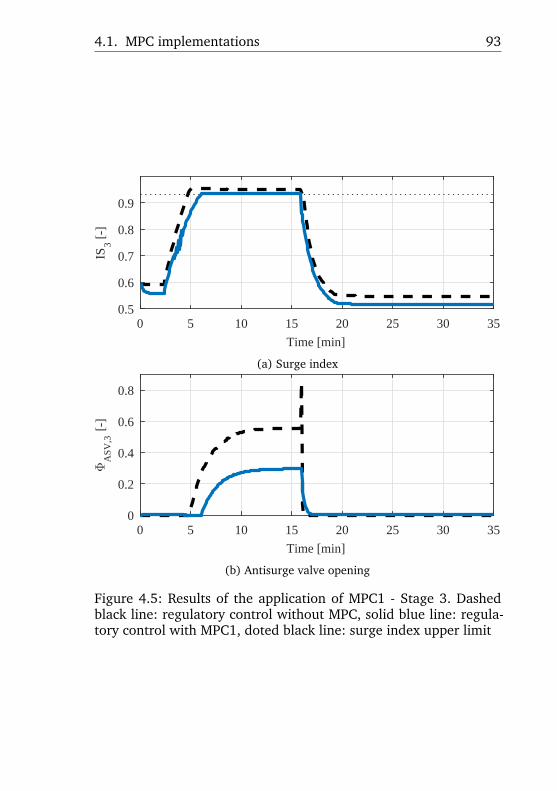
4.1. MPC implementations 93
0 5 10 15 20 25 30 35
Time [min]
0.5
0.6
0.7
0.8
0.9
IS3 [
-]
(a) Surge index
0 5 10 15 20 25 30 35
Time [min]
0
0.2
0.4
0.6
0.8
ΦA
SV,3
[-]
(b) Antisurge valve opening
Figure 4.5: Results of the application of MPC1 - Stage 3. Dashedblack line: regulatory control without MPC, solid blue line: regula-tory control with MPC1, doted black line: surge index upper limit

94 Chapter 4. Implementation and Results
0 5 10 15 20 25 30 35
Time [min]
5.5
6
6.5
7
pin
[ba
r]
Figure 4.6: Results of the application of MPC1 - inlet header pres-sure. Dashed black line: regulatory control without MPC, solid blueline: regulatory control with MPC1
0 5 10 15 20 25 30 35
Time [min]
160
165
170
175
pou
t [ba
r]
Figure 4.7: Results of the application of MPC1 - outlet header pres-sure. Dashed black line: regulatory control without MPC, solid blueline: regulatory control with MPC1
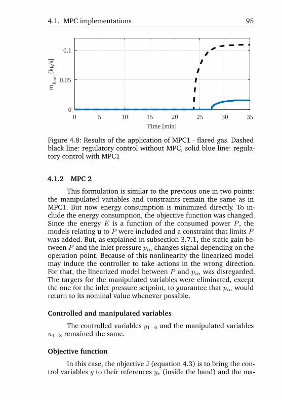
4.1. MPC implementations 95
0 5 10 15 20 25 30 35
Time [min]
0
0.05
0.1m
flar
e [kg
/s]
Figure 4.8: Results of the application of MPC1 - flared gas. Dashedblack line: regulatory control without MPC, solid blue line: regula-tory control with MPC1
4.1.2 MPC 2
This formulation is similar to the previous one in two points:the manipulated variables and constraints remain the same as inMPC1. But now energy consumption is minimized directly. To in-clude the energy consumption, the objective function was changed.Since the energy E is a function of the consumed power P , themodels relating u to P were included and a constraint that limits Pwas added. But, as explained in subsection 3.7.1, the static gain be-tween P and the inlet pressure pin changes signal depending on theoperation point. Because of this nonlinearity the linearized modelmay induce the controller to take actions in the wrong direction.For that, the linearized model between P and pin was disregarded.The targets for the manipulated variables were eliminated, exceptthe one for the inlet pressure setpoint, to guarantee that pin wouldreturn to its nominal value whenever possible.
Controlled and manipulated variables
The controlled variables y1 - 6 and the manipulated variablesu1 - 8 remained the same.
Objective function
In this case, the objective J (equation 4.3) is to bring the con-trol variables y to their references yr (inside the band) and the ma-
96 Chapter 4. Implementation and Results
nipulated variable u1 to its target while minimizing the control vari-ation \Delta \bfu and the energy consumption E.
J = [\^y - yr]TQy[\^y - yr] + \Delta \bfu TQu\Delta \bfu
+ (u1 - pnomin )TQt(u1 - pnomin ) + EQE (4.3)
Control tuning
The weight for the minimization of the energy consumptionwas set to 1 and added as QE . The new diagonal matrices are:
Qy = diag([100, 100, 100, 100, 100, 100, 1])
Qu = diag([0.1, 0.001, 1, 1, 1, 1, 1, 1])
Qt = 0.0005
QE = 1
In this formulation, \^y are also kept in a band, as explained in section2.1.4. So, if 0 \leq \^y \leq 0.93 then Qy = 0.
Constraints
Since the energy consumption is a function of the power con-sumption, the lower and upper limits for power were added. As thepower value is normalized, the lower limit is 0 and the upper limitis 1. All other constraints were maintained.
Results
The results obtained with the application of the second MPCformulation are shown in figures 4.9 to 4.14. In the figures, thedashed black lines represent the system’s performance with the reg-ulatory system only and the blue solid lines are the results of theapplication of the MPC2 formulation. In figures 4.3a, 4.4a, and 4.5athe doted black lines are the maximum limit of the surge indexes.These results are very similar to the ones obtained with the firstMPC formulation, presented in subsection 4.1.1. Even though thepower consumption was reduced, the controller could not keep thesurge indexes below their upper limit.
This formulation was also tested with different tunings andin some cases the control actions were too aggressive while in oth-ers they were smooth but the system’s response was too slow. Thus,

4.1. MPC implementations 97
it was also difficult to tune manually the weights in MPC2. Thissuggests the use of a different method for this tuning, which is pre-sented hereafter.

98 Chapter 4. Implementation and Results
0 5 10 15 20 25 30 35
Time [min]
0.7
0.8
0.9
1
IS1 [
-]
(a) Surge index
0 5 10 15 20 25 30 35
Time [min]
0
0.5
1
ΦA
SV,1
[-]
(b) Antisurge valve opening
Figure 4.9: Results of the application of MPC2 - Stage 1. Dashedblack line: regulatory control without MPC, solid blue line: regula-tory control with MPC2, doted black line: surge index upper limit

4.1. MPC implementations 99
0 5 10 15 20 25 30 35
Time [min]
0.6
0.7
0.8
0.9
1
IS2 [
-]
(a) Surge index
0 5 10 15 20 25 30 35
Time [min]
0
0.2
0.4
0.6
0.8
ΦA
SV,2
[-]
(b) Antisurge valve opening
Figure 4.10: Results of the application of MPC2 - Stage 2. Dashedblack line: regulatory control without MPC, solid blue line: regula-tory control with MPC2, doted black line: surge index upper limit

100 Chapter 4. Implementation and Results
0 5 10 15 20 25 30 35
Time [min]
0.5
0.6
0.7
0.8
0.9
IS3 [
-]
(a) Surge index
0 5 10 15 20 25 30 35
Time [min]
0
0.2
0.4
0.6
0.8
ΦA
SV,3
[-]
(b) Antisurge valve opening
Figure 4.11: Results of the application of MPC2 - Stage 3. Dashedblack line: regulatory control without MPC, solid blue line: regula-tory control with MPC2, doted black line: surge index upper limit

4.1. MPC implementations 101
0 5 10 15 20 25 30 35
Time [min]
5.5
6
6.5
7p
in [
bar]
Figure 4.12: Results of the application of MPC2 - inlet header pres-sure. Dashed black line: regulatory control without MPC, solid blueline: regulatory control with MPC2
0 5 10 15 20 25 30 35
Time [min]
160
165
170
175
pou
t [ba
r]
Figure 4.13: Results of the application of MPC2 - outlet header pres-sure. Dashed black line: regulatory control without MPC, solid blueline: regulatory control with MPC2

102 Chapter 4. Implementation and Results
0 5 10 15 20 25 30 35
Time [min]
0
0.05
0.1
mfl
are [
kg/s
]
Figure 4.14: Results of the application of MPC2 - flared gas. Dashedblack line: regulatory control without MPC, solid blue line: regula-tory control with MPC2
4.1.3 MPC with satisficing tuning
The results shown in the previous subsections suggest thatthe MPC could be a good approach to improve the compression sys-tem control, however tuning the parameters of the weight matricesQy, Qu, and Qt have showed to be difficult, mainly because of thedifferent dynamics and ranges that each variable has. To overcomethis problem, the satisficing MPC tuning was used. The results ofMPC1 were not improved with this technique, so only the results ofMPC2 are shown in this section. The satisficing technique requiresthat acceptable ranges for each variable are defined, as explainedin section 2.3. For this problem, the ranges were chosen as:
F\Delta usat = Nu[0.12 202 0.052 0.052 0.052 0.052 0.052 0.052]T
Futsat = Nu[52]T
F ysat = N [0.012 0.012 0.012 0.012 0.012 0.012]T
FEsat = N [0.52]T
where:
F\Delta usat - factor used to calculate the weights of Qu for the control
increments \Delta \bfu ,
Futsat - factor used to calculate the weight of Qt for the target error
(u1 - pnomin ),
4.1. MPC implementations 103
F ysat - factor used to calculate the weights of Qy for the reference
error [\^y - yr],
FEsat - factor used to calculate the weight of QE for energy con-
sumption minimization E,
Nu - control horizon,
N - prediction horizon.
Results
The results obtained by tuning MPC2 with the satisficing tun-ing technique are shown in figures 4.15 to 4.21. The performanceof MPC1 was not improved by the technique so only the results ob-tained with MPC 2 are shown. The black dashed lines correspond tothe compression system with the regulatory control only. The bluedash-dot lines correspond to the results of the application of MPC2with manual tuning while the red solid lines are the results of theapplication of MPC2 with satisficing tuning.

104 Chapter 4. Implementation and Results
0 5 10 15 20 25 30 35
Time [min]
0.7
0.8
0.9
1
IS1 [
-]
(a) Surge index
0 5 10 15 20 25 30 35
Time [min]
0
0.5
1
ΦA
SV,1
[-]
(b) Antisurge valve opening
Figure 4.15: Results of the satisficing tuning applied on MPC2 -Stage 1. Dashed black line: regulatory control without MPC, solidblue line: regulatory control with MPC2 tuned manually, solid redline: regulatory control with MPC2 tuned with the satisficing tech-nique, doted black line: surge index upper limit
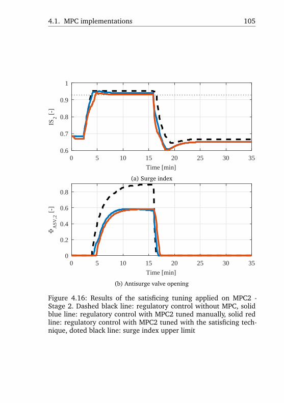
4.1. MPC implementations 105
0 5 10 15 20 25 30 35
Time [min]
0.6
0.7
0.8
0.9
1
IS2 [
-]
(a) Surge index
0 5 10 15 20 25 30 35
Time [min]
0
0.2
0.4
0.6
0.8
ΦA
SV,2
[-]
(b) Antisurge valve opening
Figure 4.16: Results of the satisficing tuning applied on MPC2 -Stage 2. Dashed black line: regulatory control without MPC, solidblue line: regulatory control with MPC2 tuned manually, solid redline: regulatory control with MPC2 tuned with the satisficing tech-nique, doted black line: surge index upper limit
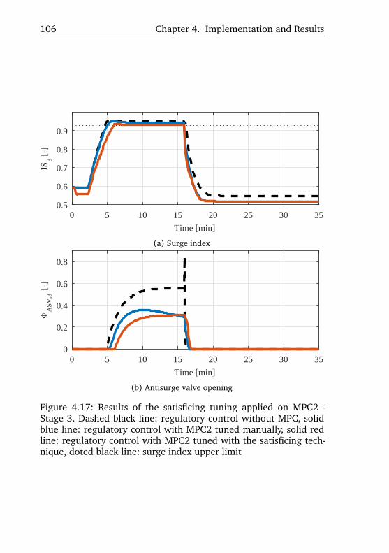
106 Chapter 4. Implementation and Results
0 5 10 15 20 25 30 35
Time [min]
0.5
0.6
0.7
0.8
0.9
IS3 [
-]
(a) Surge index
0 5 10 15 20 25 30 35
Time [min]
0
0.2
0.4
0.6
0.8
ΦA
SV,3
[-]
(b) Antisurge valve opening
Figure 4.17: Results of the satisficing tuning applied on MPC2 -Stage 3. Dashed black line: regulatory control without MPC, solidblue line: regulatory control with MPC2 tuned manually, solid redline: regulatory control with MPC2 tuned with the satisficing tech-nique, doted black line: surge index upper limit

4.1. MPC implementations 107
The performance of the controller was improved by the satis-ficing tuning. The overshoot of the surge indexes was reduced, andthe MPC2 was able to maintain the indexes at their limit in steadystate.
0 5 10 15 20 25 30 35
Time [min]
5.5
6
6.5
7
pin
[ba
r]
Figure 4.18: Results of the satisficing tuning applied on MPC2 - in-let header pressure. Dashed black line: regulatory control withoutMPC, solid blue line: regulatory control with MPC2 tuned manually,solid red line: regulatory control with MPC2 tuned with the satisfic-ing technique
0 5 10 15 20 25 30 35
Time [min]
160
165
170
175
pou
t [ba
r]
Figure 4.19: Results of the satisficing tuning applied on MPC2 - out-let header pressure. Dashed black line: regulatory control withoutMPC, solid blue line: regulatory control with MPC2 tuned manually,solid red line: regulatory control with MPC2 tuned with the satisfic-ing technique

108 Chapter 4. Implementation and Results
0 5 10 15 20 25 30 35
Time [min]
0
0.05
0.1
mfl
are [
kg/s
]
Figure 4.20: Results of the satisficing tuning applied on MPC2 -flared gas. Dashed black line: regulatory control without MPC, solidblue line: regulatory control with MPC2 tuned manually, solid redline: regulatory control with MPC2 tuned with the satisficing tech-nique
0 5 10 15 20 25 30 35
Time [min]
0.6
0.7
0.8
0.9
1
Nom
aliz
ed p
ower
[-]
Figure 4.21: Results of the satisficing tuning applied on MPC2 - con-sumed power. Dashed black line: regulatory control without MPC,solid blue line: regulatory control with MPC2 tuned manually, solidred line: regulatory control with MPC2 tuned with the satisficingtechnique
Figure 4.21 shows the power consumed by the compressionsystem and, even though MPC2 minimizes it directly, there is no sig-nificant difference in the consumption. Due to the changes executedin pin, both MPC controllers were able to decrease the amount of

4.2. Robustness analysis 109
Table 4.1: MPC performance comparison
Regulatory MPC1 MPC2 MPC2manual satisficing
Energy consumption 100% 96.24% 97.92% 97.01%Flared gas 100% 9.22% 5.15% 5.15%Recycled gas 100% 60.07% 66.23% 63.46%
flared gas.Table 4.1 summarizes the performance of the proposed MPCs.
The results obtained by simulating the system without any MPCcontroller were considered the worst case scenario, therefore theyrepresent 100% of energy consumption, gas flaring, and gas recy-cling. For example, the application of the MPC2 algorithm causethe system to recycle only 63.46% of the total amount of gas recy-cled by the system with the regulatory control only. The applicationof MPC1 resulted in a smaller energy consumption than the appli-cation of MPC2 because MPC1 recycled less gas. However, MPC1fail to keep the surge indexes below their maximum limit, as shownin figures 4.3a to 4.5a. MPC2 spends more energy recycling moregas to keep IS \leq 0.93, as shown in figures 4.15a to 4.17a. The per-formance comparison presented in table 4.1 shows little differencebetween MPC2 manual and MPC2 satisficing. The main advantageof the satisficing tuning technique is that it provided a satisfactorytune for the MPC controller faster then other heuristic techniques.
4.2 ROBUSTNESS ANALYSIS
To further investigate the proposed solutions a robustnessanalysis was made. To do so, errors in critical parameters were in-troduced. These parameters were selected based on the practicalknowledge of the process engineers regarding the studied compres-sion system:
\bullet Molecular weight of the gas - \pm 15\%
\bullet Moment of inertia of the compressors turbines - \pm 40\%
\bullet Antisurge valves coefficients - \pm 20\%
\bullet Scrubber volumes - \pm 40\%

110 Chapter 4. Implementation and Results
The linearized prediction model was obtained at the sameequilibrium point used by the manufacturer to obtain the compres-sor’s data sheet, that is the same gas molecular weight, flow rate,and pressure to be the nominal values defined by the manufacturer.The scenario presented in the previous section was simulated 50times. Each time, randomly chosen errors were added to the listedparameters. In each simulation the prediction model remained thesame but the plant was different. The error added to each parame-ter was randomly chosen in a rectangular distribution between thedefined limits. Figures 4.22a to 4.28 show the results of the robust-ness test applied to MPC2. The black solid lines represent the regu-latory control results and the colored dashed lines are the results ofthe MPC2 in several simulations. Even though there are differencesin the results, they are very similar. The optimization problem cre-ated to obtain the control increments was never infeasible and MPCcontroller worked properly at every simulation.

4.2. Robustness analysis 111
0 5 10 15 20 25 30 35
Time [min]
0.7
0.8
0.9
1
IS1 [
-]
(a) Surge index
0 5 10 15 20 25 30 35
Time [min]
0
0.5
1
ΦA
SV,1
[-]
(b) Antisurge valve opening
Figure 4.22: Results of the robustness test - stage 1. Solid black line:regulatory control without MPC, colored dashed lines: regulatorycontrol with MPC2, doted black line: surge index upper limit
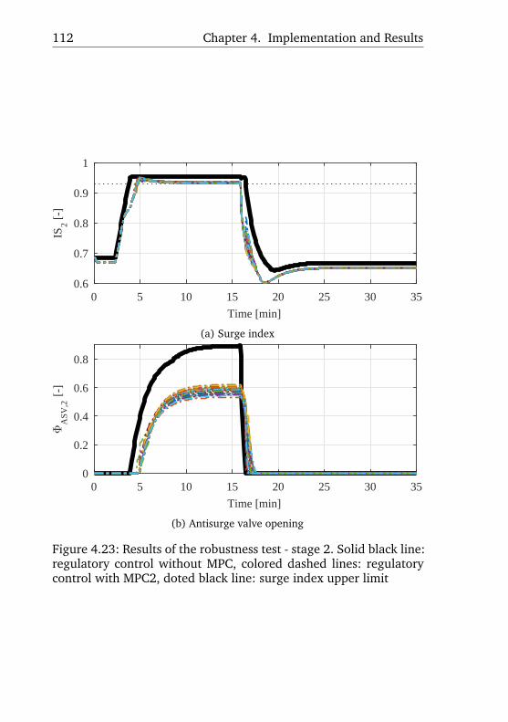
112 Chapter 4. Implementation and Results
0 5 10 15 20 25 30 35
Time [min]
0.6
0.7
0.8
0.9
1
IS2 [
-]
(a) Surge index
0 5 10 15 20 25 30 35
Time [min]
0
0.2
0.4
0.6
0.8
ΦA
SV,2
[-]
(b) Antisurge valve opening
Figure 4.23: Results of the robustness test - stage 2. Solid black line:regulatory control without MPC, colored dashed lines: regulatorycontrol with MPC2, doted black line: surge index upper limit

4.2. Robustness analysis 113
0 5 10 15 20 25 30 35
Time [min]
0.5
0.6
0.7
0.8
0.9
IS3 [
-]
(a) Surge index
0 5 10 15 20 25 30 35
Time [min]
0
0.2
0.4
0.6
0.8
ΦA
SV,3
[-]
(b) Antisurge valve opening
Figure 4.24: Results of the robustness test - stage 3. Solid black line:regulatory control without MPC, colored dashed lines: regulatorycontrol with MPC2, doted black line: surge index upper limit

114 Chapter 4. Implementation and Results
0 5 10 15 20 25 30 35
Time [min]
5.5
6
6.5
7
pin
[ba
r]
Figure 4.25: Results of the robustness test - inlet header pressure.Solid black line: regulatory control without MPC, colored dashedlines: regulatory control with MPC2
0 5 10 15 20 25 30 35
Time [min]
160
165
170
175
pou
t [ba
r]
Figure 4.26: Results of the robustness test - outlet header pressure.Solid black line: regulatory control without MPC, colored dashedlines: regulatory control with MPC2

4.2. Robustness analysis 115
0 5 10 15 20 25 30 35
Time [min]
0
0.05
0.1m
flar
e [kg
/s]
Figure 4.27: Results of the robustness test - flared gas. Solid blackline: regulatory control without MPC, colored dashed lines: regula-tory control with MPC2
0 5 10 15 20 25 30 35
Time [min]
0.6
0.7
0.8
0.9
1
Nom
aliz
ed c
onsu
med
pow
er [
-]
Figure 4.28: Results of the robustness test - consumed power. Solidblack line: regulatory control without MPC, colored dashed lines:regulatory control with MPC2
With these results it is expected that the MPC2 could be ap-plied to the real compression system. The same test was performedwith the MPC1, but in this case the results showed that this solutionis less robust. The optimization problem was infeasible in the ma-jority of the simulations and the MPC algorithm could not calculatethe control actions for control the system.

116 Chapter 4. Implementation and Results
4.3 FINAL COMMENTS
This chapter presented the implementations of two MPC con-trollers and the results of their application. It also presented theresults of the applications of the satisficing tuning technique andthe results of a robustness test.
In the first MPC formulation, the total energy is minimized in-directly as the controller drives the manipulated variables to valuesthat minimize the power consumption. This formulation was triedso that the nonlinearities between the power consumption and theinlet header pressure would not affect the system’s performance,since the model that relates them would not be used. But theseresults were not satisfactory and could not be improved by the sat-isficing tuning. MPC1 also failed the robustness test.
The second MPC formulation had better results than the firstone. In MPC2 formulation the energy consumption was includedin the objective function so it could be minimized directly. MPC2’sperformance was improved by the application of the satisficing tech-nique. MPC2 passed the robustness test because it worked well evenwhen critical parameters of the model were changed.

5 CONCLUSIONS
In this dissertation a MPC controller was proposed to improvethe performance of an compression system. For that, a detailed de-scription of the system’s mathematical model was presented, alongwith the analysis of the system’s behavior and of the potential con-trolled and manipulated variables to be used by the MPC controllersto achieve the control objectives. A tuning technique was also testedto improve the system’s performance and a robustness test was per-formed. Two MPC formulations were presented. In the first one,the energy consumption is minimized indirectly while in the secondformulation the energy consumption is minimized directly in the ob-jective function. Only the second formulation achieved the controlobjectives and proved to be robust to the disturbance applied.
The main contributions of this dissertation are:
\bullet the modeling and analysis of a complete compression systemfrom a real oil production platform,
\bullet the formulation of a MPC controller as a control layer abovethe regulatory system, running at a higher sampling period,
\bullet the application of a tuning technique that improved the sys-tem’s performance.
In the literature, several compressor models can be found, butthey usually describe the compression on a single stage. In this dis-sertation, the modeled system consists of two parallel 3-stage com-pressors with an inlet header and an outlet header. Chapter 3 pre-sented the modeling and analysis of the compression system. Thismodeling resulted in two publications [25, 35].
This work also presented a MPC controller capable of prevent-ing surge and while minimizing energy consumption. Chapter 2 pre-sented important concepts used in the MPC formulation along withthe satisficing technique to tune the MPC controller. The applica-tion of this technique improved the MPC controller’s performance.The possibility of implementing the MPC as a control layer abovethe regulatory PID controllers with a greater sampling time was in-vestigated. Even though the surge phenomena occurs in less than asecond and the MPC was set to run every 5 seconds, the MPC’s pre-dictive ability allowed the controller to drive the system to a saferoperation point, preventing surge.
Regarding practical outcome, because of the success of theproposed control strategy in the simulated plant, the algorithm will
117

118 Chapter 5. Conclusions
be implemented in a real-time control software. After exhaustivetestings, it may be applied on a real oil and gas production platform.Regarding academic follow-up, it will be performed a test to assessthe MPC controller’s performance in a scenario of a compressiontrain shutdown.

REFERENCES
1 AGUIAR, M. A.; CODAS, A.; CAMPONOGARA, E. Systemwideoptimal control of offshore oil production networks with timedependent constraints. IFAC-PapersOnLine, v. 48, n. 6, p. 200 – 207,2015.
2 GRAVDAHL, J. T. Modeling and Control of Surge and RotatingStall in Compressors. Thesis (PhD) — NTNU-Norwegian University ofScience and Technology, Trondheim, Norway, 1998.
3 RAMUSSEN, P. C.; KURZ, R. Centrifugal compressor applications -ustream and midstream. 38th Turbomachinery Symposium, 2009.
4 GRAVDAHL, J. T. et al. Modeling for surge control of centrifugalcompressors:comparison with experiment. Proceedings of the 39th IEEEConference on Decision and Control, 2000.
5 BUDINIS, S.; THORNHILL, N. F. Control of centrifugal compressorsvia model predictive control for enhanced oil recovery applications.Proceeding of the 2nd IFAC Workshop on Automatic Control in OffshoreOil and Gas Production, Florianopolis, SC, Brasil, 2015.
6 TORRISI, G. et al. Model predictive control approaches forcentrifugal compression systems. Proceedings of the 54th IEEEConference on Decision and Control, 2015.
7 GREITZER, E. M. Surge and rotating stall in axial flowcompressors—part i: Theoretical compression system model. Journalof Engineering for Power - Transactions of the ASME, p. 190–198, 1976.
8 GRAVDAHL, J. T.; EGELAND, O. Speed and surge control for a loworder centrifugal compressor model. Model Identification and Control,vol.19, n1, 13-29, 1998.
9 BOINOV, K. O. et al. Surge control of the electrically drivencentrifugal compressor. IEEE TRANSACTIONS ON INDUSTRYAPPLICATIONS, VOL. 42, NO. 6, NOVEMBER/DECEMBER 2006, 2006.
10 DORMIDO, S. Una revisión de las tecnologías de control predictivobasado en modelos en la industria. Wokshop sobre estado y perspectivasdel control predictivo, Valladolid, Spain, 1987.
11 OVERVAG, T. F. Centrifugal Compressor Load Sharing with the useof MPC. Thesis (PhD) — NTNU-Norwegian University of Science andTechnology, Trondheim, Norway, 2013.
119

120 References
12 CORTINOVIS, A. et al. Model predictive anti-surge control ofcentrifugal compressors with variable-speed drives. Proceedings of the2012 IFAC Workshop on Automatic Control in Offshore Oil and GasProduction, Trondheim, Norway, 2012.
13 SMEULERS, J.; BOUMAN, I. W.; ESSEN, H. van. Model predictivecontrol of compressor installations. Proceedings of the IMeche 1999,Trondheim, Norway, 1999.
14 SANTOS, J. E. W. dos. Método de Ajuste para MPC baseado EmMulti-Cenários para Sistemas Não Quadrados. Dissertation (Master) —Universidade Federal do Rio Grande do Sul, Porto Alegre, 2016.
15 GARRIGA, J. L.; SOROUSH, M. Model predictive control tuningmethods: A review. Industrial and Engineering Chemistry Research,n. 49, p. 3505–3515, 2010.
16 LIMA, M. L. et al. Distributed Satisficing MPC. IEEE Transactionson Control Systems Technology, v. 23, n. 1, p. 305–312, 2015.
17 BERGH, L. G.; MACGREGOR, J. F. Constrained minimum variancecontrollers: Internal model structure and robustness properties. Ind.Eng. Chem. Res., v. 26, p. 1558–1564, 1987.
18 PALMOR, Z. Properties of optimal stochastic control systems withdead-time. Automatica, v. 18, p. 107–116, 1982.
19 CAMACHO, E.; BORDONS, C. Model Predictive Control. Berlin:Springer, 2007.
20 FLESCH, R. C. C. Contribuicoes ao Controle de SistemasMonovariaveis e Multivariaveis com Atraso de Transporte. Thesis (PhD)— Universidade Federal de Santa Catarina, 2012.
21 LIMA, D. M. et al. Improving Robustness and DisturbanceRejection Performance with Industrial MPC. Congresso Brasileiro deAutomática, 2014.
22 MORARI, M.; LEE, J. H.; GARCIA, C. E. Model Predictive Control.New Jersey: Prentice Hall, 2002.
23 M.P.BOYCE et al. Practical aspects of centrifugal compressorssurge and surge control. Proceedings of the Twelfth TurbomachinerySymposium, 1983.

References 121
24 HANSEN, C. Dynamic Simulation of Compressor Control Systems.Thesis (PhD) — Aalborg University Esbjerg, Niels Bohrs vej 86700Esbjerg, Denmark, 2008.
25 PLUCENIO, A. et al. Modeling and control of a gas compressionstation used in an oil platform. Congresso Brasileiro de Automática,Vitoria, ES, Brasil, 2016.
26 HAFAIFA, B. R. A.; MOULOUD, G. Modeling of surge phenomenain a centrifugal compressor: experimental analysis for control. SystemsScience and Control Engineering, 2 : 1, 632 - 641, 2014.
27 GRAVDAHL, J. T. et al. Modeling for surge control in free-spoolcentrifugal compresssors:experimental validation. JOURNAL OFPROPULSION AND POWER, 2004.
28 JIANG, J. K. W.; DOUGAL, R. A. Dynamic centrifugal compressormodel for system simulation. Journal of Power Sources, 2005.
29 PAPARELLA, F. et al. Load sharing optimization of parallelcompressors. European Control Conference, ECC, 2013.
30 NIEUWENHUIZEN, M. Parameter analysis and identification ofthe Greitzer model by analogy with the Van der Pol equation. Thesis(PhD) — Technische Universiteit Eindhoven, Department MechanicalEngineering, Dynamics and Control Technology Group, De Rondom 70,5612 AP Eindhoven, Netherlands, 2008.
31 BOHAGEN, B. Active surge control of centrifugal compressionsystems. Thesis (PhD) — NTNU-Norwegian University of Science andTechnology, Trondheim, Norway, 2007.
32 DRESSER. Control Valve Sizing Handbook. Huston: DresserMasoneilan, 2009.
33 PLUCENIO, A. Desenvolvimento de Tecnicas de Controle Nao Linearpara Elevacao de Fluidos Multifasicos. Thesis (PhD) — Programade Pos-Graduacao em Engenharia de Automacao e Sistemas, DAS,Universidade Federal de Santa Catarina, Florianopolis-SC-Brasil, 2010.
34 YANG, B. P.; PLUCENIO, A. Practical non-linear model predictivecontrol pnmpc: Algorithm implementations. Congresso Brasileiro deAutomática, Vitoria, ES, Brasil, 2016.

122 References
35 PLUCENIO, A. et al. Advanced control applied to a gascompression station of a production platform. Congresso Brasileiro deAutomática, Vitoria, ES, Brasil, 2016.