
Vibration Testing & Modal Identification Jean-Claude Golinval
Model identification and Smart structural vibration Control using
∞H controller
M.Sridevi, P.Madhavasarma
Department of Electronics& Instrumentation Engineering,
SASTRA UNIVERSITY, Thanjavur- 613401 T.N, India,
Emails: [email protected], [email protected] Abstract- A smart structure plays a vital role in aerospace applications and robotics and other
applications. It presents many challenging control problems due to their non-linear dynamic
behavior. The Objective of this work is to design a controller that minimizes the structural vibration
using H∞ controller. Vibration as a measured parameter has been used to evaluate model of a non-
linear process (piezoelectric actuator and sensor) at different modes .The model was generated using
an ARMAX technique. By selecting appropriate weighting functions ∞H controller were designed
based on mixed sensitivity approach using singular loop shaping method. The performance of ∞H
controller was compared with LQG controller based on vibration reduction. From the results it is
observed that the H∞ controller is the best suited for smart structural process.
Index terms: ∞H controller, ARMAX, smart structure, LQG, weighting function, loop shaping,
weighting function,
I INTRODUCTION
In recent times structures that have self sensing action and reaction capabilities known as smart
structures play a vital role in active control of vibration. There have been significant advances in
modern control theory with robust controllers gaining widespread recognition in field of
aerospace and robotics. The goal of robust analysis is to find a Multivariable Stability Margin
(MSM) seen by the uncertainties using a proper non conservative and analytical tool.
The ∞H control strategy as compared to classical control techniques provides an advanced
method and perspective for designing control systems. This is accomplished by shaping the
INTERNATIONAL JOURNAL ON SMART SENSING AND INTELLIGENT SYSTEMS, VOL. 3, NO. 4, DECEMBER 2010
655
frequency response characteristics of the plant according to prespecified performance
specifications in the form of frequency dependent weighting functions. Chopra [1] has used
piezoelectric materials for sensing and actuation. Costain et al [2] have developed practical
methods for vibration control of industrial equipment. Herman [3] has analyzed modeling of
smart structure using piezoelectric material as sensor/actuator. Yang et al [4] have suggested on
the location of sensor and actuator and there effects in control. Choi et al [5] have designed and
implemented various control methods such as Variable Structure Control (VSC), Gaudenzi et al
[6] has suggested genetic algorithm and fuzzy for piezoelectric bonded structures. Raymond et
al [7] have determined the optimal constant Output Feedback Gains for linear multivariable
Systems. Sridevi et al [8-9] have designed state and output feedback control for cantilever beam.
Umapathy et al [10] have developed the periodic output feedback controllers for disturbance
rejection for piezoelectric bonded structures. Brief discussion on ∞H control problems have
been discussed by various authors. They have not discussed about weighting function selection
for controller design [11-15].The present work aims at identification of model using ARMAX
technique and design of ∞H controller that provides robust stability to structural uncertainties
for the smart structure to suppress the fundamental vibration mode of a smart cantilever beam
using MATLAB software.
II EXPERIMENTAL SETUP
The experimental set-up for smart structure control is shown in Figure 1. This consists of a
cantilever beam made of aluminum bonded with one pair of collocated piezoelectric patches as
sensor/actuator at the fixed end. To apply disturbance a piezoelectric patch is bonded at the free
end of the beam. The conditioned piezo sensor output was given as analog input to dSPACE
controller board. The control algorithm was developed using SIMULINK and implemented in
real time on dSPACE system using RTW and dSPACE Real Time Interface tools. The controller
output was directed to piezoelectric actuator through driving amplifier. The dimensions and
properties of the beam and piezoelectric patches are given in Tables 1 and 2.
M.Sridevi and P.Madhavasarma, MODEL IDENTIFICATION AND SMART STRUCTURAL VIBRATION CONTROL USING CONTROLLER
656

Figure 1 Experimental setup for smart structure control.
Table 1: Properties and dimensions of the Aluminum beam
Length (m) l 0.3 Width (m) b 0.0127 Thickness (m) bt 0.0023 Young’s modulus (Gpa) bE 71
Density (kg/m3) bρ 2700
Natural frequencies (Hz) f 31.7, 200 Damping ratio ξ 0.0524 Damping constants α , β 2.8676 , 4.5231x10⁻⁴
Table 2: Properties and dimensions of piezoelectric sensor/actuator
length (m) pl 0.0765 Width (m) b 0.0127
Thickness (m) at 0.005 Young’s modulus (Gpa) pE 47.62
Density (kg/m3) pρ 7500
Piezoelectric strain constant (m V-1)
31d -247x10-12
Piezoelectric stress constant (V m N-1) 31g -9x10⁻³
INTERNATIONAL JOURNAL ON SMART SENSING AND INTELLIGENT SYSTEMS, VOL. 3, NO. 4, DECEMBER 2010
657
III MODEL IDENTIFICATION
Identification and control is gaining wide spread recognition due to accurate modeling obtained
through system identification techniques [16-20]. The actual output of the system and predicted
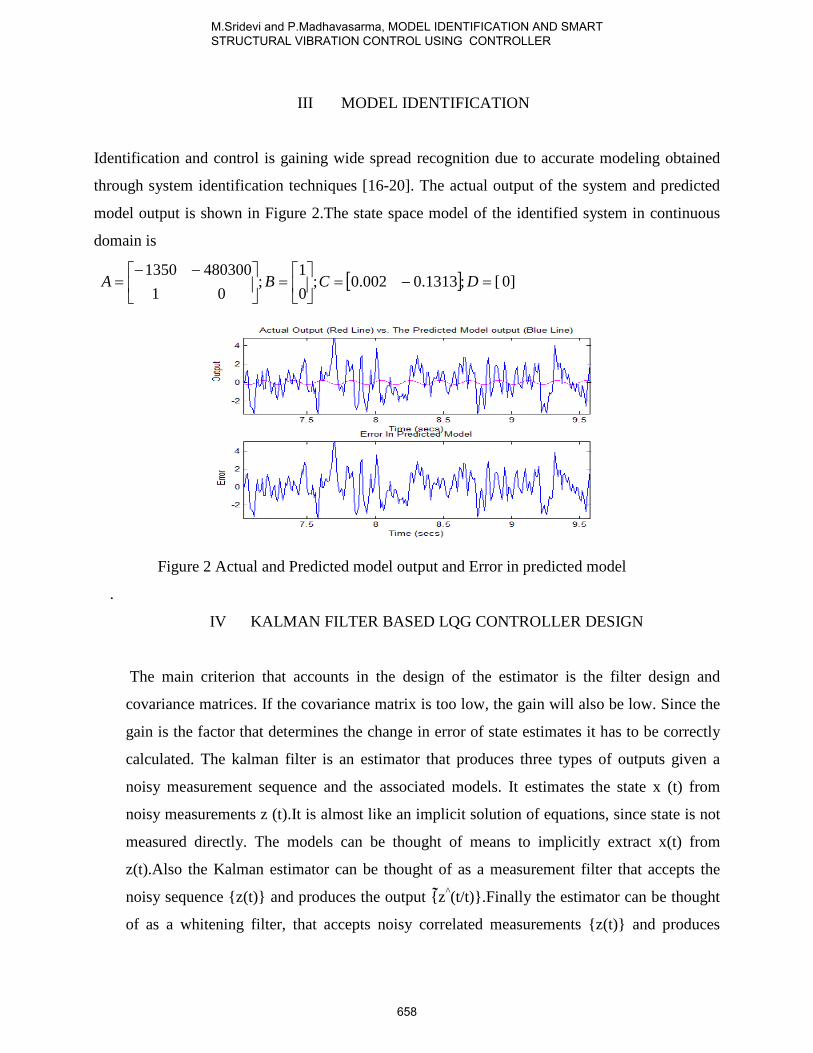
model output is shown in Figure 2.The state space model of the identified system in continuous
domain is
[ ] [;1313.0002.0;01
;01
4803001350=−=
=
−−= DCBA 0]
Figure 2 Actual and Predicted model output and Error in predicted model
.
IV KALMAN FILTER BASED LQG CONTROLLER DESIGN
The main criterion that accounts in the design of the estimator is the filter design and
covariance matrices. If the covariance matrix is too low, the gain will also be low. Since the
gain is the factor that determines the change in error of state estimates it has to be correctly
calculated. The kalman filter is an estimator that produces three types of outputs given a
noisy measurement sequence and the associated models. It estimates the state x (t) from
noisy measurements z (t).It is almost like an implicit solution of equations, since state is not
measured directly. The models can be thought of means to implicitly extract x(t) from
z(t).Also the Kalman estimator can be thought of as a measurement filter that accepts the
noisy sequence {z(t)} and produces the output {z ^(t/t)}.Finally the estimator can be thought
of as a whitening filter, that accepts noisy correlated measurements {z(t)} and produces
M.Sridevi and P.Madhavasarma, MODEL IDENTIFICATION AND SMART STRUCTURAL VIBRATION CONTROL USING CONTROLLER
658
uncorrelated or white equivalent measurements {e(t)}, the innovation sequence. The
operation of a Kalman filter algorithm can be viewed as a predictor-corrector algorithm.
First, at time t , before receiving the measurement {z(t)}, with the previous filtered estimate
x(t-1/t-1) and covariance P(t-1/t-1) it finds the best estimate of the state, based on (t-1) data
samples. This is the “prediction phase” of algorithm. The state space model is used to predict
the state estimate x (t-1/t-1) and associated error covariance P(t/t-1). Once the prediction
based on the model is completed it calculates the innovation covariance and Kalman gain G.
As soon as the measurement at time t, that is z(t), becomes available, the innovation e(t) is
determined. Now this the correction phase of the innovation. The old or predicted, state
estimate x (t/t-1) is used to form the filtered ,or corrected, state estimate x (t/t) and P(t/t).Here
the error, or innovation, is the difference between the actual measurement and the predicted
measurement Z(t/t-1).The innovation is weighted by the gain G(t) to correct the old state
estimate(predicted) x (t/t-1).The associated error covariance is corrected as well. The
algorithm then awaits the next measurement at time (t+1). In the absence of
measurement the state space model is used to perform the prediction, since it provides the
best estimate of the state .The first term of the predicted covariance P (t/t-1) relates to
uncertainty in predicting the state using the model. The second term indicates the increase in
error covariance, due to the contribution of the process noise. The corrected covariance
equation indicates the predicted error covariance equation or the uncertainty due to
prediction, which is decreased by the update, there by producing the corrected error
covariance P (t/t).The controller gain is designed through the selection of controller poles
through root locus analysis for the smart structure model
jjjj Bwxx +Φ=+ )()1( (1)
A discrete measurement is given by:
1)1()1(1 ++++ += jjjj vxHZ (2)
Where nj .....2,1,0=
jw = white noise with zero mean represented by Q,
INTERNATIONAL JOURNAL ON SMART SENSING AND INTELLIGENT SYSTEMS, VOL. 3, NO. 4, DECEMBER 2010
659

Q = Process Noise
jv = sensor noise represented by R
The algorithm is as follows:
One step Estimate Prediction:
)/(1ˆ jjjj xx Φ=+ (3)
Measurement update:
)1()1()/()1()/()1( ++++ += jjjjjj EGxx here, (4)
)/1()1()1()1( jjjjj xHZE ++++ −= (5)
Estimate error covariance prediction:
BBQPP jjjjjj ′+Φ′Φ=+ )/()()/()1( P (6)
Innovations Measurement Residual Variance:
1jα + = RHPH jjjj +′ +++ )1()/1()1( (7)
Kalman’s gain:
)1(1
)/()1( ** +−
+ ′= jjjj HPG α (8)
Estimate Error Measurement Update:
)/1()1()1()/1()1/1( jjjjjjjj PHGPP ++++++ −= (9)
Filter output:
))(( )/(/)/( ′−−= jjjjjjjj xxxxEP (10)
Predictor:
))(( )/1(1/11)/1( ′−−= +++++ jjjjjjjj xxxxEP (11)
Estimator output:
M.Sridevi and P.Madhavasarma, MODEL IDENTIFICATION AND SMART STRUCTURAL VIBRATION CONTROL USING CONTROLLER
660
11/)1(1/1 +++++ += jjjjjj EGxx (12)
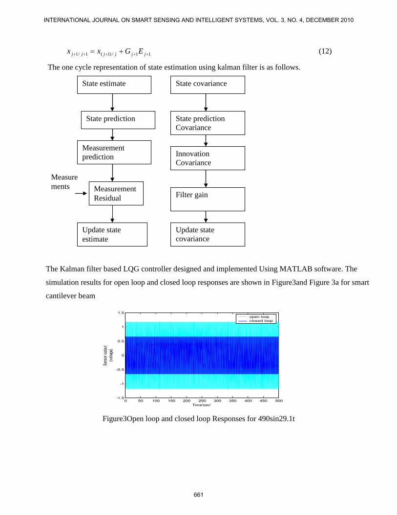
The one cycle representation of state estimation using kalman filter is as follows.
The Kalman filter based LQG controller designed and implemented Using MATLAB software. The
simulation results for open loop and closed loop responses are shown in Figure3and Figure 3a for smart
cantilever beam
0 50 100 150 200 250 300 350 400 450 500-1.5
-1
-0.5
0
0.5
1
1.5
Time'sec'
Sens
or ou
tput
(volta
ge)
open loopclosed loop
Figure3Open loop and closed loop Responses for 490sin29.1t
State covariance
Measurement Residual
Update state estimate
State prediction Covariance
Innovation Covariance
Filter gain
Update state covariance
State estimate
State prediction
Measurement prediction Measure
ments
INTERNATIONAL JOURNAL ON SMART SENSING AND INTELLIGENT SYSTEMS, VOL. 3, NO. 4, DECEMBER 2010
661
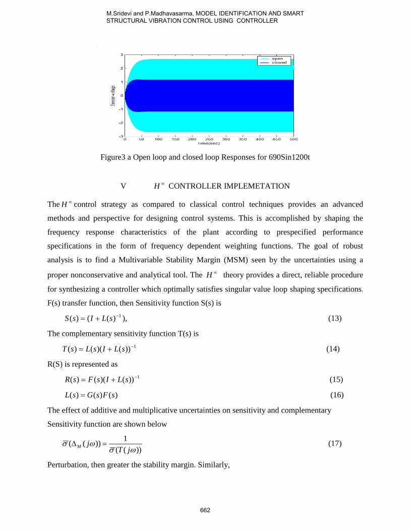
Figure3 a Open loop and closed loop Responses for 690Sin1200t
V ∞H CONTROLLER IMPLEMETATION The ∞H control strategy as compared to classical control techniques provides an advanced
methods and perspective for designing control systems. This is accomplished by shaping the
frequency response characteristics of the plant according to prespecified performance
specifications in the form of frequency dependent weighting functions. The goal of robust
analysis is to find a Multivariable Stability Margin (MSM) seen by the uncertainties using a
proper nonconservative and analytical tool. The ∞H theory provides a direct, reliable procedure
for synthesizing a controller which optimally satisfies singular value loop shaping specifications.
F(s) transfer function, then Sensitivity function S(s) is
1)(()( −+= sLIsS ), (13)
The complementary sensitivity function T(s) is
1))()(()( −+= sLIsLsT (14)
R(S) is represented as
1))()(()( −+= sLIsFsR (15)
)()()( sFsGsL = (16)
The effect of additive and multiplicative uncertainties on sensitivity and complementary
Sensitivity function are shown below
))((
1))((ωσ
ωσjT
jM =∆ (17)
Perturbation, then greater the stability margin. Similarly,
M.Sridevi and P.Madhavasarma, MODEL IDENTIFICATION AND SMART STRUCTURAL VIBRATION CONTROL USING CONTROLLER
662

))((
1))((ωσ
ωσjR
jA =∆ (18)
The stability margins of the control system via singular value are
)())(( 12 ωωσ jwjR −≤ (19)
)())(( 13 ωωσ jwjT −≤ (20)
Where 2w and 3w are weightages on the control and output signal respectively.
The representation of the plant with the weighting functions is shown in Figure 4.
.
Figure 4Augmented plant
The shape of uncertainty regions defined by the amplitude ratio and phase shift bounds does not
have a simple geometry and therefore cause difficulties during analysis. This problem is
overcome by specifying a disk, large enough to encapsulate the original uncertainty region. The
disk has only one parameter, its radius, )(~ ωal , which is a function of frequency. That is, at each
frequency value, there will be a corresponding disk. It is expected that )(~ ωal will increase with
frequency, as it is easier to characterize the process when they are near the steady state. Although
the disks provide a convenient means of describing uncertainties, their use results in more
conservative description of uncertainties. Thus use of disks of radius )(~ ωal yields a description of
a set ℑ of processes about the nominal model and this can be written mathematically as:
INTERNATIONAL JOURNAL ON SMART SENSING AND INTELLIGENT SYSTEMS, VOL. 3, NO. 4, DECEMBER 2010
663

{ })(~)(~)(: ωωω appp ljGjGG ≤−=ℑ
where pG is the real process, pG~ is the nominal model of the process and )(~ ωal is the radius of
the disk used to describe uncertainties between the real and the nominal process at each frequency
value. In other words , any member of the set ℑ satisfies :
)()(~)( ωωω jljGjG app +=
where )(~ ωal is the uncertainty associated with the model )(~ ωjGp and is known as the additive
uncertainty. Further the additive uncertainty is bounded according to :
)(~)( ωω jljla ≤
Alternately, the plant uncertainties can be modeled using multiplicative uncertainty description
as below :
≤−
=ℑ )(~)(~
)(~)(: ω
ω
ωωjl
jG
jGjGG m
p
ppp
Here , any member ℑ satisfies
))(1)((~)( ωωω jljGjG mpp +=
where )( ωjlm is the multiplicative uncertainty description that has the following bounds
)(~)( ωω jljl mm ≤
The additive and multiplicative uncertainty bounds are related by the following equation :
)(~)(~)(~ ωωω jljGjl ma = .One of the performance objectives of controller design is to keep the
error between the controlled output and the set-point as small as possible, when the closed-loop
system is affected by external signals. Thus, to be able to asses the performance of a particular
controller, we need to be able to quantify the relationship between this error, the process and the
controller. One such quantifying measure is the sensitivity function )(sε and its counter part
complementary sensitivity function )(sη .The sensitivity function )(sε relates the effect of
disturbance d(s) on the process output Y(s). The complementary sensitivity function )(sη relates
the effect of the set-point R(s) on the process output Y(s). Thus, for a conventional feedback
control system, these functions are defined as follows:
M.Sridevi and P.Madhavasarma, MODEL IDENTIFICATION AND SMART STRUCTURAL VIBRATION CONTROL USING CONTROLLER
664
)()(1)()(
)()()(
)()(11
)()()(
sGsGsGsG
sRsYs
sGsGsdsYs
PC
PC
PC
+==
+==
η
ε
Also )(sη = 1- )(sε . For perfect disturbance rejection, )(sε = 0 and for perfect set-point tracking
)(sη = 1. Both these function values are bound between 0 and 1.
If there is process noise N(s) ≠ 0, then
)()(1)()(
)()()()(
sGsGsGsG
sNsRsYs
PC
PC
+=
−=η
)(sη is also affected by noise N(s). In this case, )(sη has to be made small so as to reduce the
influence of random inputs. In other words we want )(sη = 0 or equivalently )(sε = 1. This
means that good set-point tracking and disturbance rejection has to be traded off against the noise
suppression. Design of controller involves the selection of the weighting functions satisfying
singular value loop specifications and the stability margins. The weighting functions over the
desired frequency range are not related directly to performance characteristics. Numerous trial
weighting functions are required in order to obtain desired performance characteristics. The
weighting functions to the error signal, control signal, output signal are represented as 1w , 2w and
3w respectively. The weighting function 1w is used to reshape the frequency response
characteristics and is chosen in such away that 1w act as a low pass filter. No weightage is given
to control signal 2w . The weighting function 3w is decided based on the multiplicative
uncertainty present in the plant. The plant is augmented with the decided weighting functions.
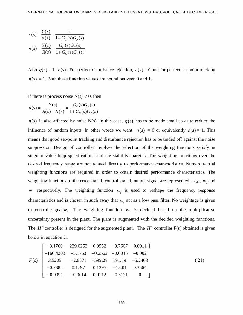
The ∞H controller is designed for the augmented plant. The ∞H controller F(s) obtained is given
below in equation 21
3.1760 239.0253 0.0552 0.7667 0.0011160.4203 3.1763 0.2562 0.0046 0.002
( ) 3.5205 2.6571 599.28 191.59 5.24680.2384 0.1797 0.1295 13.01 0.35640.0091 0.0014 0.0112 0.3121 0
F s
− − − − − − − = − − − − − − − −
( 21)
INTERNATIONAL JOURNAL ON SMART SENSING AND INTELLIGENT SYSTEMS, VOL. 3, NO. 4, DECEMBER 2010
665
The ∞H controller obtained after performing model reduction is giving in equation 22
12.98 0.28 0.0518 0.33130.2801 6.2403 195.7742 0.0036
( )0.0518 195.7742 0.2165 0.0007
0.3313 0.0036 0.0007 0
F s
− − − − = − − − −
(22)
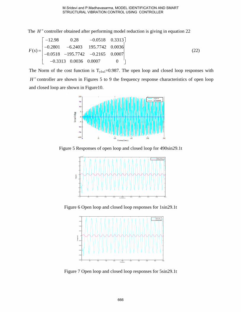
The Norm of the cost function is Ty1u1=0.987. The open loop and closed loop responses with ∞H controller are shown in Figures 5 to 9 the frequency response characteristics of open loop
and closed loop are shown in Figure10.
Figure 5 Responses of open loop and closed loop for 490sin29.1t
0 50 100 150 200 250 300 350 400 450 500-10
-8
-6
-4
-2
0
2
4
6
8x 10
-3
Time(sec)
Voltag
e(volt)
Open loop Closed loop
Figure 6 Open loop and closed loop responses for 1sin29.1t
0 50 100 150 200 250 300 350 400 450 500-0.05
-0.04
-0.03
-0.02
-0.01
0
0.01
0.02
0.03
0.04
Time(sec)
Volta
ge(v
olt)
Open loopClosed loop
Figure 7 Open loop and closed loop responses for 5sin29.1t
M.Sridevi and P.Madhavasarma, MODEL IDENTIFICATION AND SMART STRUCTURAL VIBRATION CONTROL USING CONTROLLER
666
0 50 100 150 200 250 300 350 400 450 500-5
-4
-3
-2
-1
0
1
2
3
4
Time(sec)
Vol
tage
(vol
t)
Open loopClosed loop
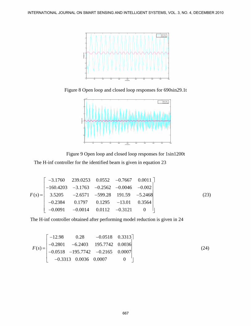
Figure 8 Open loop and closed loop responses for 690sin29.1t
0 50 100 150 200 250 300 350 400 450 500-3
-2
-1
0
1
2
3x 10
-3
Time(sec)
Volta
ge(v
olt)
Open loopClosed loop
Figure 9 Open loop and closed loop responses for 1sin1200t
The H-inf controller for the identified beam is given in equation 23
3.1760 239.0253 0.0552 0.7667 0.0011160.4203 3.1763 0.2562 0.0046 0.002
( ) 3.5205 2.6571 599.28 191.59 5.24680.2384 0.1797 0.1295 13.01 0.35640.0091 0.0014 0.0112 0.3121 0
F s
− − − − − − − = − − − − − − − −
(23)
The H-inf controller obtained after performing model reduction is given in 24
12.98 0.28 0.0518 0.33130.2801 6.2403 195.7742 0.0036
( )0.0518 195.7742 0.2165 0.0007
0.3313 0.0036 0.0007 0
F s
− − − − = − − − −
(24)
INTERNATIONAL JOURNAL ON SMART SENSING AND INTELLIGENT SYSTEMS, VOL. 3, NO. 4, DECEMBER 2010
667
10-1
100
101
102
103
104
-180
-160
-140
-120
-100
-80
-60
-40
-20Frequency Response
Magnitu
de (dB)
open loopclosed loop
Bode Diagram
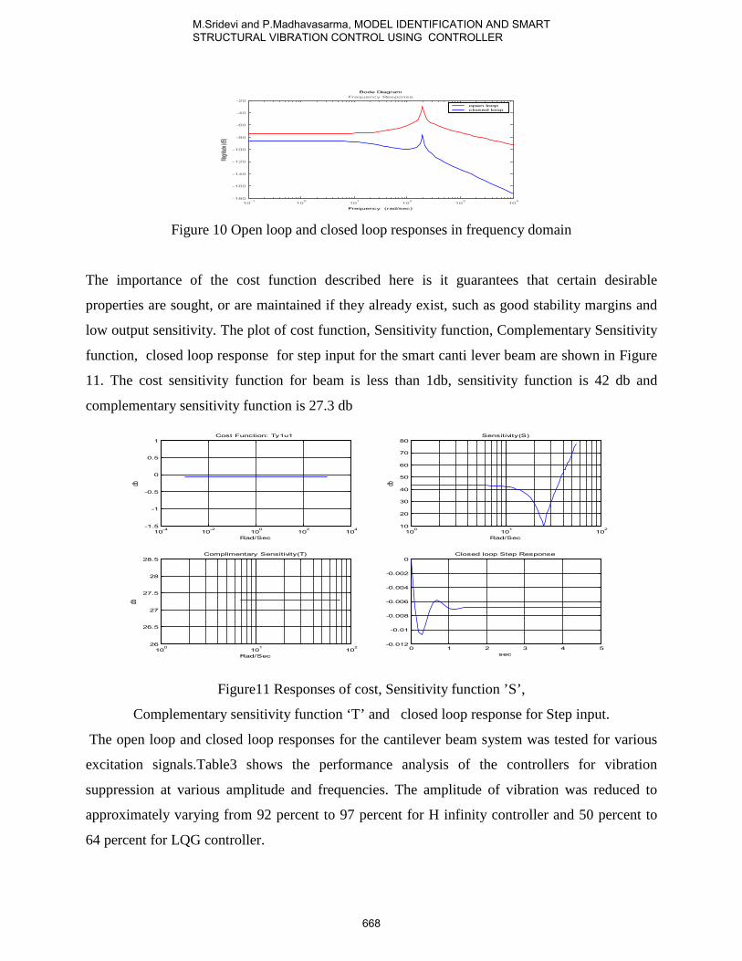
Frequency (rad/sec) Figure 10 Open loop and closed loop responses in frequency domain
The importance of the cost function described here is it guarantees that certain desirable
properties are sought, or are maintained if they already exist, such as good stability margins and
low output sensitivity. The plot of cost function, Sensitivity function, Complementary Sensitivity
function, closed loop response for step input for the smart canti lever beam are shown in Figure
11. The cost sensitivity function for beam is less than 1db, sensitivity function is 42 db and
complementary sensitivity function is 27.3 db
10-4
10-2
100
102
104
-1.5
-1
-0.5
0
0.5
1Cost Function: Ty1u1
Rad/Sec
db
100
101
102
10
20
30
40
50
60
70
80Sensitivity(S)
Rad/Sec
db
100
101
102
26
26.5
27
27.5
28
28.5Complimentary Sensitivity(T)
Rad/Sec
db
0 1 2 3 4 5-0.012
-0.01
-0.008
-0.006
-0.004
-0.002
0Closed loop Step Response
sec
Figure11 Responses of cost, Sensitivity function ’S’,
Complementary sensitivity function ‘T’ and closed loop response for Step input.
The open loop and closed loop responses for the cantilever beam system was tested for various
excitation signals.Table3 shows the performance analysis of the controllers for vibration
suppression at various amplitude and frequencies. The amplitude of vibration was reduced to
approximately varying from 92 percent to 97 percent for H infinity controller and 50 percent to
64 percent for LQG controller.
M.Sridevi and P.Madhavasarma, MODEL IDENTIFICATION AND SMART STRUCTURAL VIBRATION CONTROL USING CONTROLLER
668
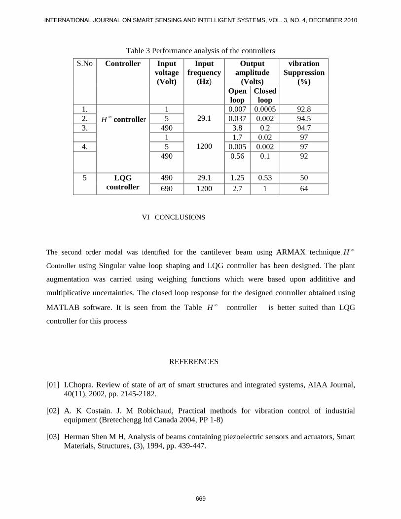
Table 3 Performance analysis of the controllers S.No Controller Input
voltage (Volt)
Input frequency
(Hz)
Output amplitude
(Volts)
vibration Suppression
(%) Open loop
Closed loop
1. ∞H controller
1 29.1
0.007 0.0005 92.8 2. 5 0.037 0.002 94.5 3. 490 3.8 0.2 94.7 1
1200
1.7 0.02 97 4. 5 0.005 0.002 97 490 0.56 0.1 92
5 LQG controller
490 29.1 1.25 0.53 50 690 1200 2.7 1 64
VI CONCLUSIONS
The second order modal was identified for the cantilever beam using ARMAX technique. ∞H
Controller using Singular value loop shaping and LQG controller has been designed. The plant
augmentation was carried using weighing functions which were based upon addititive and
multiplicative uncertainties. The closed loop response for the designed controller obtained using
MATLAB software. It is seen from the Table ∞H controller is better suited than LQG
controller for this process
REFERENCES
[01] I.Chopra. Review of state of art of smart structures and integrated systems, AIAA Journal, 40(11), 2002, pp. 2145-2182.
[02] A. K Costain. J. M Robichaud, Practical methods for vibration control of industrial equipment (Bretechengg ltd Canada 2004, PP 1-8)
[03] Herman Shen M H, Analysis of beams containing piezoelectric sensors and actuators, Smart Materials, Structures, (3), 1994, pp. 439-447.
INTERNATIONAL JOURNAL ON SMART SENSING AND INTELLIGENT SYSTEMS, VOL. 3, NO. 4, DECEMBER 2010
669
[04] Yang S. M, and Lee Y. J, Optimization of non-collocated sensor/actuator location and feedback gain in control systems Smart Materials, Structures, (8), 1993, pp. 96-102.
[05] Choi S.B, Chong C.C and Lee C.H Position tracking control of a smart flexible structure featuring a piezoflim actuator, Journal of Guidance, Control and Dynamics, 19(6), 1996, pp. 1364-1369.
[06] P Gaudenzi. E Fantini., K Vlasis. and J. Charis Gantes. Genetic algorithm optimization for the active control of a beam by means of PZT actuators, Journal of Intelligent Material Systems and Structures, 9, 1998, pp. 291-300.
[07] A, Raymond. On the determination of the optimal constant Output Feedback Gains for linear Multivariable Systems IEEE transactions on Automatic control, vol Ac-15:1 146-142. 1970.
[08] M Sridevi. J, Balasubramani. And M Umapathy. Design & Implementation of State and Output Feedback Control for Piezoelectric Bonded Beam Proceedings of ISSS 2005 International Conference on Smart Materials, Structures and Systems, Bangalore, 28th to 30th, 2005, Vol 1, pp SA 148 – SA 155
[09] M Sridevi., .M Umapathy, Vibration control of smart cantilever beam using DS1104, M.Tech Thesis NIT Trichy 2005.
[10] .M Umapathy, B Bandyopadhyay. Vibration control of flexible beam through smart structure concept using periodic output feedback System Science Journal, 26(1), 2000, pp. 43-66
[11] N Rubin. And D Limbeer.. H-inf identification for robust control In proceedings of American control conference Pages 2040-2044, Chicago,June 1994.
[12] J.C Doyle,. K Glover,, P.P Khargonekar, and Francis, B.A.State-Space Solutions 18 of Standard H2 and H-inf Control Problems IEEE Transactions on Automatic Control, Vol. AC-29, 831-847.
[13] J.L Crassidis, D.J Leo, D.J Inman, and D.J Mook. Robust Identification and Vibration Suppression of a Flexible Structure Journal of Guidance, Control, and Dynamics, Vol. 17, No. 5, 921-928.
[14] M. G Saponov, D. J. N Limebeer, and R. Y Chiang,. Simplifying the H-inf Theory via Loop-Shifting, Matrix-Pencil and Descriptor Concepts Int. J.Control, 50, No. 6, pp. 2467–2488.
[15] D Edberg. and A.Bicos, Design and Development of Passive and Active Damping Concepts for Adaptive Structures Conference on Active Materials and Adaptive Structures by G. Knowles, IOP Publishing Ltd., Bristol, UK, 377-382.
[16] R.N Juang. Applied System Identification Prentice Hall, Englewood Cliffs, NJ. 1994.
M.Sridevi and P.Madhavasarma, MODEL IDENTIFICATION AND SMART STRUCTURAL VIBRATION CONTROL USING CONTROLLER
670

[17] P.Madhavasarma, S. Sundaram. Model based tuning of controller for non linear hemispherical tank processes. Instrum. Sci&Technol. 2007, 35, 681-689
[18] P.Madhavasarma, S Sundaram, Model based tuning of controller for non linear spherical tank processes. Instrum. Sci&Technol. 2008, 36, 420-431.
[19] P.Madhavasarma,; S. Sundaram,. Model based evaluation of controller using flow sensor for conductivity process. 2007, 36, 420-431. J. Sensors & Transducers, 79, 1164-1172.
[20] P.Madhavasarma, S. Sundaram, Leak Detection and Model Analysis for Nonlinear Spherical Tank Process Using Conductivity Sensor. J. Sensors & Transducers, 2008, 89, pp. 71-76.
:
INTERNATIONAL JOURNAL ON SMART SENSING AND INTELLIGENT SYSTEMS, VOL. 3, NO. 4, DECEMBER 2010
671