Model-based Clustering with Dissimilarities: A Bayesian Approach
30
Model-based Clustering with Dissimilarities: A Bayesian Approach 1 Man-Suk Oh Ewha University, Seoul Adrian Raftery University of Washington, Seattle Working Paper no. 38 Center for Statistics and the Social Sciences University of Washington December 16, 2003 1 Man-Suk Oh is Associate Professor of Statistics, Department of Statistics, Ewha Wom- ens University, Seoul 120-750, Korea. Email: [email protected]. Adrian E. Raftery is Professor of Statistics and Sociology, Department of Statistics, University of Washing- ton, Box 354322, Seattle WA 98195-4322. Email: [email protected]; Web: www.stat.washington.edu/raftery. Oh’s research was supported by research funds from KOSEF R04-2002-00-0046-0, and Raftery’s research was supported by NIH Grant 1R01CA094212-01 and ONR Grant N00014-01-10745.
Transcript of Model-based Clustering with Dissimilarities: A Bayesian Approach

Model-based Clustering with Dissimilarities: A Bayesian
Approach 1
Man-Suk OhEwha University, Seoul
Adrian RafteryUniversity of Washington, Seattle
Working Paper no. 38Center for Statistics and the Social Sciences
University of Washington
December 16, 2003
1Man-Suk Oh is Associate Professor of Statistics, Department of Statistics, Ewha Wom-
ens University, Seoul 120-750, Korea. Email: [email protected]. Adrian E. Raftery
is Professor of Statistics and Sociology, Department of Statistics, University of Washing-
ton, Box 354322, Seattle WA 98195-4322. Email: [email protected]; Web:
www.stat.washington.edu/raftery. Oh’s research was supported by research funds from KOSEF
R04-2002-00-0046-0, and Raftery’s research was supported by NIH Grant 1R01CA094212-01 and
ONR Grant N00014-01-10745.

Abstract
A Bayesian model-based clustering method is proposed for clustering objects on the basisof dissimilarites. This combines two basic ideas. The first is that the objects have latentpositions in a Euclidean space, and that the observed dissimilarities are measurements ofthe Euclidean distances with error. The second idea is that the latent positions are gen-erated from a mixture of multivariate normal distributions, each one corresponding to acluster. We estimate the resulting model in a Bayesian way using Markov chain MonteCarlo. The method carries out multidimensional scaling and model-based clustering simul-taneously, and yields good object configurations and good clustering results with reasonablemeasures of clustering uncertainties. In the examples we studied, the clustering results basedon low-dimensional configurations were almost as good as those based on high-dimensionalones. Thus the method can be used as a tool for dimension reduction when clusteringhigh-dimensional objects, which may be useful especially for visual inspection of clusters.
We also propose a Bayesian criterion for choosing the dimension of the object config-uration and the number of clusters simultaneously. This is easy to compute and worksreasonably well in simulations and real examples.
Key Words: Cluster Analysis, Mixture Model, Markov chain Monte Carlo, Model selec-tion.

Contents
1 Introduction 1
2 Model for Clustering with Dissimilarities 3
3 Posterior Inference 4
3.1 Markov chain Monte Carlo . . . . . . . . . . . . . . . . . . . . . . . . . . . . 43.2 Non-Identifiability . . . . . . . . . . . . . . . . . . . . . . . . . . . . . . . . 6
4 A Bayesian Selection Criterion for Configuration of Dimension and the
Number of Clusters 6
5 Examples 9
5.1 Simulation Examples . . . . . . . . . . . . . . . . . . . . . . . . . . . . . . . 95.2 Lloyds Bank Data . . . . . . . . . . . . . . . . . . . . . . . . . . . . . . . . . 135.3 Leukemia Data . . . . . . . . . . . . . . . . . . . . . . . . . . . . . . . . . 155.4 Yeast Cell Cycle Data . . . . . . . . . . . . . . . . . . . . . . . . . . . . . . 18
6 Discussion 21
List of Tables
1 MIC values for Leukemia data for p = 2, 3, 49 . . . . . . . . . . . . . . . . . 182 MIC values for Yeast data for p = 2, 3, 16. . . . . . . . . . . . . . . . . . . . 203 Three Sources of Errors in Clustering with Dissimilarities . . . . . . . . . . . 23
List of Figures
1 Scatterplots of true objects in the simulation data . . . . . . . . . . . . . . . 102 Plots of MIC for p = 2 in the six simulation data sets . . . . . . . . . . . . . 113 Scatterplots of the estimated object configuration and the classification from
BMCD in the six simulation data sets . . . . . . . . . . . . . . . . . . . . . . 124 Scatterplots of the estimated object configuration and the component density
functions from BMCD for the Lloyds Bank data. . . . . . . . . . . . . . . . . 145 Distances for some selected individuals in the Leukemia data . . . . . . . . . 166 MICs for Leukemia data with G = 1. . . . . . . . . . . . . . . . . . . . . . . 177 Three-dimensional and pairwise scatter plots for the object configuration and
their classification from BMCD for the Leukemia data . . . . . . . . . . . . . 198 Scatterplots of object configuration from BMCD with p = 2 in the Yeast data
and their classifications . . . . . . . . . . . . . . . . . . . . . . . . . . . . . . 22
i

1 Introduction
Cluster analysis is the automatic grouping of objects into groups on the basis of numerical
data consisting of measures either of properties of the objects, or of the dissimilarities be-
tween them. It was developed initially in the 1950s (e.g. Sneath 1957; Sokal and Michener
1958), and the early development was driven by problems of biological taxonomy and market
segmentation. More recently, clustering has attracted a great deal of attention as a useful
tool for grouping genes and samples in DNA microarray experiments, clustering documents
on the World Wide Web and in other text databases, and grouping pixels in medical images
so as to identify features of clinical interest.
For much of the past half-century, the majority of cluster analysis done in practice have
used heuristic methods based on dissimilarities between objects. These include hierarchical
agglomerative clustering using various between-cluster dissimilarity measures such as small-
est dissimilarity (single link), average dissimilarity (average link) or maximum dissimilarity
(complete link), the k means algorithm (MacQueen 1967), and Self-Organizing Maps (Koho-
nen 2001). These methods are relatively easy to apply and often give good results. However,
they are not based on standard principles of statistical inference, they do not take account
of measurement error in the dissimilarities, they do not provide an assessment of clustering
uncertainties, and they do not provide a statistically based method for choosing the number
of clusters.
Model-based clustering is a framework for putting cluster analysis on a principled sta-
tistical footing; for reviews see McLachlan and Peel (2000) and Fraley and Raftery (2002).
It is based on probability models in which objects are assumed to follow a finite mixture of
probability distributions such that each component distribution represents a cluster. The
model-based approach has several advantages over heuristic clustering methods. First, it
clusters objects and estimates component parameters simultaneously, avoiding well-known
biases that exist when they are done separately. Second, it provides clustering uncertainties
which is important especially for objects close to cluster boundaries. Third, the problems of
determining the number of components and the component probability distributions can be
recast as statistical model selection problems, for which principled solutions exist. Unlike
the previously mentioned heuristic clustering algorithms, however, model-based clustering
requires object coordinates rather than dissimilarities between objects as an input. Thus,
despite the important advantages of model-based clustering, it can be used only when object
coordinates are given, and not when dissimilarities are provided.
1
In many practical applications in market research, psychology, sociology, environmental
research, genomics, and information retrieval for the Web and other document databases,
data consist of similarity or dissimilarity measures on each pair of objects (Young, 1987;
Schutze and Silverstein, 1997; Tibshirani et al. 1999; Buttenfield, 2002; Condon et al., 2002;
Courrieu, 2001; Elvevag and Storms, 2002; Priem et al., 2002; Welchew et al., 2002; Ren
and Frymier, 2003). Examples of such data include the co-purchase of items in a market,
disagreements between votes made by pairs of politicians, the execution of links between
pairs of web pages, the existence or intensity of social relationships between pairs of families,
and the overlap of university applications by high school graduates.
Even when object coordinates are given, visual display of clusters in low dimensional
space is often desired since it may provide useful information about the relationships be-
tween the clusters and the underlying data generation process (Hedenfalk et al, 2002; Yin,
2002; Nikkila, 2002). One way to reduce the dimensionality of objects for visual display
in lower dimensional space is multidimensional scaling (MDS). In MDS, objects are placed
in a Euclidean space while preserving the distance between objects in the space as well as
possible.
There are many MDS techniques in the literature. Recently Oh and Raftery (2001)
proposed a Bayesian MDS (BMDS) method using Markov chain Monte Carlo. This provided
good estimates of the object configuration in the cases studied, as well as a Bayesian criterion
for choosing the object dimension. However, they did not consider clustering and hence
clustering has to be done separately with the estimated object configuration from MDS.
In this paper, we develop a model-based clustering method for dissimilarity data. We
assume that an observed dissimilarity measure is equal to the Euclidean distance between the
objects plus a normal measurement error. We model the unobserved object configuration as
a realization of a mixture of multivariate normal distributions, each one of which corresponds
to a different cluster. We carry out Bayesian inference for the resulting hierarchical model
using Markov chain Monte Carlo (MCMC). The resulting method combines MDS and model-
based clustering in a coherent framework.
There are three sources of uncertainty in model-based clustering with dissimilarites: (a)
measurement errors in the dissimilarities; (b) error in estimating the object configuration;
and (c) clustering uncertainty. Heuristic clustering methods that cluster directly from dis-
similarities, such as hierarchical agglomerative clustering and self-organizing maps, do not
take account of sources (a) and (c), while source (b) does not arise there. As an alternative,
one may consider a two-stage procedure which estimates the object configuration in the first
2

stage, using a heuristic MDS method or BMDS, and carries out model-based clustering in
the second stage. Sequential application of heuristic MDS and model-based clustering takes
account of source (c) but not of sources (a) and (b). Sequential application of Bayesian
MDS and model-based clustering considers sources (a) and (c), but separately rather than
together; it does not consider source (b). In contrast, our approach accounts for all three
sources of uncertainty simultaneously. Simultaneous estimation of the errors is important,
because errors in the dissimilarity measures and/or the estimated configuration can affect
the clustering and the clustering uncertainties, as we will show by example.
Other important issues are the choice of the number of clusters and of the dimension of
the objects. Oh and Raftery (2001) proposed an easily computed Bayesian criterion called
MDSIC for choosing object dimension. We extend this to determine the number of clusters
as well. The resulting criterion can be computed easily from MCMC output.
Section 2 describes our model for dissimilarities, the mixture model for the object config-
uration, and the prior distributions we use. Section 3 describes Bayesian estimation for this
model using MCMC. The Bayesian criterion for choosing the dimension and the number of
clusters is given in Section 4, while the method is applied to several simulated and real data
sets in Section 5. A summary and discussions are given in Section 6.
2 Model for Clustering with Dissimilarities
Let δij denote the dissimilarity measure between objects i and j, which is assumed to be
functionally related to p unobserved attributes of the objects. Let xi = (xi1, ..., xip) denote
an unobserved vector representing the values of the attributes possessed by object i.
As in Oh and Raftery (2001), we model the true dissimilarity measure δij as the distance
between objects i and j in a Euclidean space, i.e., δij =√
∑pk=1(xik − xjk)2. In practical
situations, the true dissimilarity measure can be different from Euclidean distance and there
can be measurement error in observations. We therefore assume that the observed dissim-
ilarity measure, dij, is equal to the true measure, δij, plus a Gaussian error. In addition,
since dissimilarity measures are typically given as positive values we restrict the observed
dissimilarity to be positive. Thus, given the Euclidean distance δij, the observed dissimilarity
measure dij is assumed to follow the truncated normal distribution
dij ∼ N(δij , σ2) I(dij > 0), i 6= j, i, j = 1, ..., n. (1)
Note that dij is related to X = {xi}, called the object configuration, only through δij. To
represent clustering, we assume that the object configuration is a sample from a mixture of
3

multivariate normal distributions,
xi ∼G∑
j=1
εj N(µj, Tj), (2)
where each component normal distribution represents a cluster.
We use the following priors for the model parameters:
σ2 ∼ IG(a, b),
(ε1, . . . εg) ∼ Dirichlet(1, ..., 1),
µj ∼ N(µj0, Tj),
Tj ∼ IW (α, Bj), (3)
where IG(a, b) is the inverse Gamma distribution with mode b/(a+1) and IW is the inverse
Wishart distribution.
One may use a more parsimonious covariance structure for Tj than the above uncon-
strained one. For instance, one may restrict Tj to be a diagonal matrix, or let T1 = · · · = TG,
or use some other parsimonious covariance model such as those commonly used in model-
based clustering (Banfield and Raftery 1993; Fraley and Raftery 2002). In that case, the
priors need to be modified accordingly.
3 Posterior Inference
3.1 Markov chain Monte Carlo
It is well known that inference for mixture models can be simplified with latent variables
which indicate the group memberships of objects. We define latent variables Ki such that
P (Ki = j) = εj and xi belongs to class j if Ki = j, so that
xi|Ki = j ∼ N(µj, Tj).
From the prior and the model, the full conditional posterior distributions (densities) given
all the other unknowns are given as
π(xi|Ki = j, others ) ∝ exp[−1/2(xi − µj)′T−1
j (xi − µj) (4)
−1
σ2
n∑
j 6=i,j=1
(δij − dij)2]
n∏
j 6=i,j=1
Φ(δij/σ) (5)
4

π(σ2| others ) ∝ (σ2)−(m/2+a+1) exp
−1
σ2(SSR/2 + b) −
∑
i>j
log Φ
(
δij
σ
)
(ε1, .., εg|others) ∼ Dirichlet(n1 + 1, ..., ng + 1), (6)
(µj| others) ∼ N(njx̄j + µj0
nj + 1,
Tj
nj + 1), (7)
(Tj| others) ∼ IW (α + nj/2, Bj + Sj/2), (8)
P (Ki = j| others) = εjφ(xi; µj, Tj)/g∑
k=1
εkφ(xi; µk, Tk), (9)
where φ and Φ are respectively pdf and cdf of the standard normal distribution, SSR =∑n
i=1
∑i−1j=1(δij − dij)
2,
nj =j∑
i=1
I(Ki = j), (10)
Sj =n∑
i=1
(xi − µj)(xi − µj)′I(Ki = j), (11)
and I is the indicator function.
Iterative generation of the unknown parameters from their full conditional distributions
for a sufficiently long time yields samples of the parameters from the joint posterior distribu-
tion, and posterior inference can be done by using the samples. When a simpler covariance
structure is used for Tj with appropriate priors, the algorithm can be easily modified since
only the generation of Tj needs to be changed.
Generation of samples from the full conditional distributions of the parameters {εj, µj, Tj}
is straightforward since the full conditional posterior distributions all have convenient forms.
However, the full conditional posterior distributions of xi and σ2 do not have closed forms,
and so we apply the Metropolis-Hastings algorithm (Hastings, 1970) to generate samples
of xi and σ2. Oh and Raftery (2001) suggested an easy random walk Metropolis-Hastings
algorithm for generating samples of xi and σ2 when G=1. Given the latent indicator variable
Ki, xi follows a one-component multivariate normal distribution. Thus, we can easily modify
the algorithm of Oh and Raftery (2001) for generating xi from its full conditional posterior
distribution in the mixture model. Given X, the distribution of σ2 does not depend on the
mixture model parameters, so that the generation of σ2 is the same in the mixture model as
in the one-component model.
To initialize the MCMC algorithm, we first run Oh and Raftery’s (2001) BMDS as a
preliminary run to obtain an initial guess for X, and then run MCLUST with this initial
guess.
5

3.2 Non-Identifiability
Euclidean distance is invariant under translation, rotation, and reflection of objects. Thus,
the dissimilarity data provide information only about the relative locations of X. In a
Bayesian context, X is identified, strictly speaking, but the absolute location and orientation
of X are defined only by the prior distribution, and in practice are very weakly identified.
As a result, the relative positions of the xi may have a tight posterior distribution, but their
absolute positions will typically have a dispersed posterior distribution.
To get around this problem of weak identification, we use a Procrustean similarity trans-
formation (Borg and Groenen 1998, Ch.12) which proceeds as follows: (i) Obtain an estimate,
X∗, of X from a preliminary run, for example the MLE or the posterior mode. (ii) Trans-
form the sample of X at each iteration of MCMC so that coordinates of X are as close as
possible to the corresponding coordinates of X∗, where the transformation is restricted to be
a composition of some or all of a translation, a rotation, and a reflection. See the Appendix
for more details. Since the transformation does not change the Euclidean distances between
pairs of xi’s, it does not change the likelihood but it approximately fixes the location and
orientation of samples of X so that X itself can be stably estimated.
There is another non-identifiability problem. A mixture of density functions is invariant
under arbitrary permutation of component labels. Thus, the posterior density function would
be invariant under arbitrary permutation of component labels unless strong prior information
is used (Stephens 2000). This may cause label switching during the MCMC iterations, hence
typical averages of MCMC samples of the parameters may yield unreasonable estimates of
the mixture parameters. To avoid this problem, we adopt the relabeling procedure suggested
by Celeux et al. (2000) at each iteration of MCMC. See the Appendix for details.
By using the two postprocessing steps, Procrustean transformation and relabelling, we
obtain stable samples of the unknown parameters from which posterior estimates can be
computed.
4 A Bayesian Selection Criterion for Configuration of
Dimension and the Number of Clusters
Posterior inference as described in the previous section presumed that the dimension, p,
of the object configuration, and the number of clusters, G, are given. These are typically
unknown, however, and we now propose a statistical method for choosing p and G. Oh
6
and Raftery (2001) suggested a dimension selection criterion for MDS, called MDSIC, which
works well with Euclidean distance measures with small or moderate error size. In this
section, we extend MDSIC and propose a new Bayesian selection criterion, named MIC, for
choosing both p and G simultaneously.
We view the overall goal of our analysis as being to choose the best object configuration
across the dimension p and the number of clusters G. We therefore base our model selection
criteria on π(XpG, p, G|D), the posterior density function of X, p, G, given data D at X =
XpG, where XpG is the best object configuration given p and G.
Note that
π(XpG, p, G|D) = c · f(D|XpG, p, G)π(XpG, p, G),
where c is a constant, f(D|XpG, p, G) =∫
f(D|XpG, p, G, σ2)π(σ2)dσ2 and π(XpG, p, G) =∫
π(XpG, p, G, Λ)dΛ are the marginal likelihood and the marginal prior of (XpG, p, G), re-
spectively. Here we use f(D| · · ·) to denote the sampling density of data D given specified
parameter values and Λ to denote the mixture model parameters (ε, µ, T ). As p or G in-
creases, the likelihood increases and it can be considered as a measure of fit. However, as
p or G increases, the prior density decreases and it can be viewed as a penalty for more
complex models.
Under equal prior probabilities for all p in pmin ≤ p ≤ pmax and for all G in Gmin ≤ G ≤
Gmax,
π(XpG, p, G|D) ∝ f(D|XpG, p, G)π(XpG|p, G).
Thus one only needs to compute the marginal likelihood and the marginal prior of X for
each p and G. Let π(XpG|D) = π(XpG, p, G|D), f(D|XpG) = f(D|XpG, p, G), and π(XpG) =
π(XpG|p, G) for notational simplicity. Oh and Raftery (2001) showed that f(D|XpG) is
approximately proportional to SSR−m/2+1pG , where SSRpG =
∑
i>j(δ(pG)ij − dij)
2 and δ(pG)ij is
the Euclidean distance between the xi and xj of XpG.
Now consider computation of π(XpG). When G = 1, with T = diag(t1, · · · , tp) and
independent IG(α, βj) priors for tj, j = 1, ..., p,
π(Xp1) = (2π)−np/2(Γ(α + n/2)/Γ(α))pp∏
j=1
βαj (βj + sj/2)−(α+n/2), (12)
where sj is the j-th diagonal component of nSx =∑
(xi− x̄)(xi− x̄)′ (Oh and Raftery 2001).
When G ≥ 2, the prior π(XpG) is not given in a closed form and needs to be estimated.
From the relationship
π(XpG) =π(XpG|Λ
∗)π(Λ∗)
π(Λ∗|XpG)(13)
7

for a fixed value Λ∗ of Λ, π(XpG) can be estimated from estimate of π(Λ∗|XpG). From Oh
(1999) it can be shown that
π(Λ∗|XpG) = E[π(ε∗|K, G)G∏
j=1
π(µ∗j |K, T ∗
j ,XpG)π(T ∗j |K, µj,XpG)], (14)
where the expectation is with respect to the joint distribution of (K, ε, µ, T ) given (XpG, p, G).
Since the conditional distributions of ε, µj, Tj are given in closed forms, π(Λ∗|XpG) can be
easily estimated by using samples of (K, ε, µ, T ) generated from MCMC algorithm. In theory
any value of Λ∗ can be used but in practice Λ∗ close to the mode of Λ seems to work well for
efficiency point of view.
However, simple comparison of the posterior of XpG can lead to the choice of large p
because of the shrinking effect. As described in Oh and Raftery (2001) there is a shrinking
effect as the dimension p increases, i.e., the scale (dispersion) of X tends to decrease as p
increases without altering the fit. This would yield larger π(XpG) for larger p even when
the likelihoods are the same and hence would favor larger p. To avoid this shrinking effect,
Oh and Raftery (2001) have suggested comparing configurations in the same dimensional
space. Specifically, they compare dimensions p and p − 1 through Xp and X∗p = (Xp−1 : 0),
a n × p matrix with the p − 1 columns equals to Xp−1 and the last column has all elements
equal to 0. Note that X∗p yields the same likelihood as Xp−1 and it may be considered as an
implantation of Xp−1 in p-dimensional space.
When G = 1, let Xp = Xp1. Since f(D|X∗p) = f(D|Xp−1),
π(Xp|D)
π(X∗p|D)
=f(D|Xp)π(Xp)
f(D|X∗p)π(X∗
p)
= [f(D|Xp)
f(D|Xp−1)
π(Xp)
π(Xp−1)][π(Xp−1)
π(X∗p)
]
= [π(Xp|D)
π(Xp−1|D)][π(Xp−1)
π(X∗p)
].
Thus, Ap = π(Xp−1)/π(X∗p) is a correction factor to the posterior density ratio of Xp and
Xp−1 for the shrinking effect. With α = 1/2 and βj = s(p)j /2n, an approximate unit infor-
mation prior, for tj, Ap is given as
−2 log Ap = −2 logπ(Xp−1)
π(X∗p)
= Hn − n log(s(p)
p
n) +
p−1∑
j=1
log(r(p)j ) + (n + 1)
log((n + 1)
(n + r(p)j )
),
where r(p)j = s
(p)j /s
(p−1)j and Hn = −(n +1) log(π) + 2 log(Γ((n+ 1)/2)). The shrinking effect
is related only to p and not to G, so we use Ap for all values of G given the same p.
8

Now we propose a selection criterion, which we call MIC, as follows. Let
MIC1G = (m − 2) log SSR1G − 2 log π(X1G)
MICpG =p∑
q=1
−2 logπ(XqG|D)
π(X∗qG|D)
(15)
=p∑
q=1
−2 logf(D|XqG)
f(D|Xq−1,G)
π(XqG)
π(Xq−1,G)− 2 log Aq (16)
= (m − 2) log(SSRpG) − 2 log π(XpG) − 2p∑
q=1
log Aq. (17)
Note that (m − 2) log(SSRpG) can be considered as a measure of fit, −2 log π(XpG) plays
the role of a penalty for complexity, and −2∑p
q=1 log Aq is a cumulative correction factor for
the shrinking effect. The values of p and G that yield the minimum of MICpG are viewed
as best.
5 Examples
We apply the proposed method, which we call BMCD, and the model selection criterion
MIC, to some simulated and real data sets.
In the simulation and Bank examples given in Sections 5.1 and 5.2, we use a general
covariance structure for Tj, and for the Leukemia and Yeast examples in Sections 5.3 and 5.4
we use the same covariance structure for Tj, i.e., T1 = T2 = · · · = TG. In all the examples,
we use x̄ as the prior mean of µj and we let α = p + 4 and Bj = (α − p − 1)Sx for the
hyper-parameters of the Inverted Wishart prior of Tj in (3), where x̄ and Sx are the average
and sample covariance matrix of the initial xi’s. Thus, we use a common mean for all µj and
a common vague prior for all Tj, and choose the scale parameter of the Inverted Wishart
distribution so that the prior mean of Tj is equal to Sx.
5.1 Simulation Examples
Six data sets with 50 objects each were generated from mixtures of bivariate normal distribu-
tions with various values of the mixture model parameters. Scatterplots of the true objects
from the six data sets are given in Figure 1. In all cases the true dimension is p = 2 but the
true numbers of clusters are different. The first set has two well-separated clusters and the
second set has three well-separated clusters. The third set has two big clusters and a small
cluster which may be considered as a group of outliers. The fourth set has two clusters with
9
o
o
oo
o
ooo
o
o
o
o
oo
o
oo
o
o
o
oo
oo
ooo
o
o
o
o
o
o
o
o
oo
o
o
o
o
o
o
o
o
o o
o
o
o
(a)dim 1
dim
2
-4 -2 0 2 4
-2-1
01
2
o
o
o o
o
o
o
o
o
oo
o
o oo
o
o
o
o
o
o
o
o
oo
ooo
o
oo
o
oo
o
o oo
o
o
o
o
o o
o
o o
o
o
o
(b)dim 1
dim
2
-4 -2 0 2 4
-20
24
o
o
o o
o
o
o
o
o
o
o
o
o oo
oo
o
o
ooo
ooooo o
o
o
oo
oo
o
o oo
o
o
o
o
o o
o
o o
o
o
o
(c)dim 1
dim
2
-4 -2 0 2 4
-4-2
02
o
o
oo
o
oo o
o
o
o
o
oo
ooo
o
o
oo
ooo
o
oo
oo
o
oo
oo
o
oo o
o
o
o
o
o oo
oo
o
o
o
(d)dim 1
dim
2
-4 -2 0 2 4
-2-1
01
23
o
o
o o
o
o
o
o
o
oo
o
o oo
o
o
o
o
o
o
oo
o o
ooo
o
ooo
oo
o
o oo
o
o
o
o
o o
o
o o
o
o
o
(e)dim 1
dim
2
-4 -2 0 2 4
-4-2
02
4
o o
oo
oo
o
oo
oo
o o
oo
o
o
o
o
o
o
oo
oo
o
oo
o
o
o
o
o
o
o
o
o ooo
o
o
o
oo
ooo
o
o
(f)dim 1
dim
2
-4 -2 0 2 4
-1.0
-0.5
0.0
0.5
Figure 1: Scatterplots of true objects in the simulation data. There are two well-separatedclusters in (a), three well-separated clusters in (b), two big clusters and a small cluster ofoutliers in (c), two clusters with different covariance structures in (d),two big clusters andtwo small clusters in a symmetric position in (e), and two close clusters in (f).
10

o
o o o o
(a)G
MIC
1 2 3 4 5
5350
5370
5390
M
o
o
o
o
o
(b)G
MIC
1 2 3 4 553
5053
7053
90
M
o
oo o
o
(c)G
MIC
1 2 3 4 5
5350
5370
5390
M
o
o oo o
(d)G
MIC
1 2 3 4 5
5350
5370
5390
M
o
o oo o
(e)G
MIC
1 2 3 4 5
5350
5370
5390
M
o
oo
oo
(f)G
MIC
1 2 3 4 5
5350
5370
5390
M
Figure 2: Plots of MIC for p = 2 in the six simulation data sets. In all cases MIC choosesthe correct number of clusters.
11
(a)dim 1
dim
2
-4 -2 0 2 4
-2-1
01
2
(b)dim 1
dim
2
-4 -2 0 2 4
-20
24
(c)dim 1
dim
2
-4 -2 0 2 4
-20
24
(d)dim 1
dim
2
-4 -2 0 2 4
-2-1
01
2
(e)dim 1
dim
2
-4 -2 0 2 4
-4-2
02
46
(f)dim 1
dim
2
-4 -2 0 2 4
-1.0
-0.5
0.0
0.5
1.0
Figure 3: Scatterplots of the estimated object configuration and the classification fromBMCD with the optimal p and G in the six simulation data sets. Different symbols representdifferent clusters.
12
different covariance structures. The fifth set has two big clusters and two small clusters that
are symmetrically located. The last set has two close clusters. For each data set, Euclidean
distances δij between pairs of objects were computed and a 50 × 50 matrix of observed dis-
similarity measures dij was obtained by generating the dij from a normal distribution with
mean δij and standard deviation 0.3, restricted to be positive.
For each data set, we applied BMCD with 20,000 MCMC iterations, of which 5,000 were
discarded for burn-in, and we computed MIC for various values of p and G. In all cases, the
MIC values for p other than 2 were much larger than the MIC value for p = 2 for every value
of G considered, so MIC correctly identifed the true dimension p = 2. Figure 2 presents
plots of MIC for various G when p = 2 for the six data sets. In all cases, MIC selected the
correct number of clusters, though MIC’s preference for the selected G was not as strong as
for p. Also, the estimated object configurations from BMCD were good, as can be seen in
Figure 3.
5.2 Lloyds Bank Data
We now consider dissimilarity measures between the careers of 80 employees of Lloyds Bank
in England during the period 1905–1950 (Stovel et al. 1996), computed using the optimal
alignment method of Sankoff and Kruskal (1983), as applied to career data by Abbott and
Hrycak (1990). Note that the dissimilarity measures in this data set are not Euclidean
distances and may not satisfy some properties of typical metric distances. Oh and Raftery
(2001) analyzed the data and MIC chose p = 8 as the optimal dimension. After removing
two outlying employees who had extremely short careers at the bank, MCLUST was applied
to the estimate of X from BMDS. It chose G = 3 and yielded a reasonable classification of
objects. The first group consisted of 16 employees who had short careers at the bank and
spent all or most of their careers at the lowest clerk rank, and the second group consisted of
30 employees who had long careers at the bank and spent all or most of their careers at the
lowest clerk rank. The third group consisted of 32 employees, 24 of whom were promoted to
managers and 8 of whom had medium length careers and ended at the clerk level.
We applied BMCD to the data with 40,000 MCMC iterations, of which the first 10,000
were discarded as burn-in. MIC chose p = 8 and G = 4, which coincides with the results
from the previous analysis. The first group was identical to the first group found in the
previous analysis. The second and the third groups were almost identical to those found in
the previous study except that the 8 employees who had medium length careers and ended
at the clerk level were clustered together with those who had long careers and ended at the
13

(a) dim 1 vs. dim 2
-3 -2 -1 0 1
-10
12
*
*
*
*
(b) dim 1 vs. dim 3
-3 -2 -1 0 1
-3-2
-10
1
*
*
*
*
(c) dim 1 vs. dim 4
-3 -2 -1 0 1
-10
12
34
**
*
*
(d) dim 2 vs. dim 3
-1 0 1 2
-3-2
-10
1
*
*
*
*
(e) dim 2 vs. dim 4
-1 0 1 2
-10
12
34
**
*
*
(f) dim 3 vs. dim 4
-3 -2 -1 0 1
-10
12
34
**
*
*
Figure 4: Scatterplots of the estimated object configuration and the component densityfunctions from BMCD for the Lloyds Bank data.
14

clerk level in BMCD, rather than with the managers. This is more satisfactory, substantively.
The fourth group consisted of the two outliers which were removed before clustering in the
previous analysis. Thus, BMCD picked up the outliers during the process and yielded a
more sensible clustering than the previous analysis. Figure 4 shows pairwise scatter plots of
object configurations and the estimated component densities for the first four coordinates.
Note that in Figure 4, the component density for the outliers has mean close to zero and a
large covariance since there are only two objects in the group and the effect of the prior is
dominant for this component. From Figure 4, it seems that BMCD gives clear separation
between clusters and takes care of the outliers.
5.3 Leukemia Data
Golub et al. (1999) used gene expression data on 50 genes and 72 acute leukemia patients to
classify the patients into different types of leukemia. The 50 genes are believed to be informa-
tive about the distinction between acute myeloid leukema (AML) and acute lymphoblastic
leukemia (ALL) in the known samples.
We follow the standardization process given by Getz et al. (2000) and compute the
Euclidean distance between genes, yielding a dissimilarity matrix similar to a correlation
matrix. Due to the standardization, the mean of each gene is set to zero and this reduces
the true dimension of the objects from 50 to 49.
Investigation of plots of dissimilarity measures between pairs of individuals shows that
there are two big groups and most dissimilarity measures between individuals in the same
group are small while those between individuals in different groups are large. Figure 5 (a) and
(b) are typical plots for individuals in the first and the second groups, respectively. However,
there are some individuals, such as numbers 12 and 55, who seem to be misclassified since
they have smaller dissimilarities with those in the different group and larger dissimilarities
with those in the same group as shown in Figure 5 (c)-(d). Also there are a few individuals
whose distances do not clearly show their closeness to either group as shown in Figure 5
(e)-(h).
In all the examples we analyzed, MIC showed a sharp drop at the same optimal value of
p for all values of G, so that the choice of G does not affect the choice of dimension. This
is because the object configurations are not much different for different Gs when the same p
is used. Thus, one may choose optimal dimension p with G = 1 and then choose optimal G
with the selected p. In other words, one may apply BMDS to choose the dimension and then
apply BMCD with the optimal dimension. This would reduce computation time significantly.
15

(a) i=3, AML
dist
ance
0 20 40 60
0.0
0.5
1.0
1.5
MM
M
MM
M
MM
MMM
M
MMMM
M
M
MM
MM
M
M
MMMM
MM
MMMMMMM
MM
M
M
MM
M
MMM
LLLL
L
LLL
LL
LLLL
L
L
LLLLL
L
LLL
(b) i=28, ALL
dist
ance
0 20 40 60
0.0
0.5
1.0
1.5
M
M
M
MMM
MM
M
M
M
M
MMMM
MM
M
MM
MMM
M
M
M
MM
M
MMMM
M
M
MM
MMMMM
M
M
MM
L
L
LL
L
LLLLLL
L
LL
L
LLLL
LL
L
LLL
(c) i=12, AML
dist
ance
0 20 40 60
0.0
0.5
1.0
1.5
M
M
MMMMM
MM
M
M
M
MMMM
MM
MMM
MMM
M
M
M
M
M
M
MMMM
M
M
MM
MM
MMM
M
M
M
ML
L
LL
L
L
LLL
LL
LL
LLL
L
LL
LLLL
L
L
(d) i=55, AML
dist
ance
0 20 40 60
0.0
0.4
0.8
1.2 M
M
M
MMMM
MM
MM
M
MMMM
MM
MMM
M
MM
MM
M
MM
M
MMMM
M
M
MM
MMMMM
M
MMM
L
L
LL
L
L
L
L
L
L
L
L
LL
L
L
LLL
LLLL
L
L
(e) i=69, ALL
dist
ance
0 20 40 60
0.0
0.4
0.8
1.2
M
M
MM
M
MM
M
MM
M
MMMMM
M
M
M
M
MMM
MMM
MM
M
M
M
M
MMM
MMMM
MM
MMMMMML
L
LL
L
LL
L
LL
L
L
LLL
L
LLLL
L
L
LLL
(f) i=25, AML
dist
ance
0 20 40 60
0.0
0.5
1.0
1.5
MM
M
MMMMMMM
M
M
MM
MM
MM
MMM
MMM
M
M
M
M
M
MMM
MMMM
MM
MMMM
MMMMML
L
LL
L
L
LLLLL
L
L
LLL
LLL
LLL
L
LL
(g) i=41, AML
dist
ance
0 20 40 60
0.0
0.4
0.8
1.2
M
M
M
MMM
M
M
MMM
M
MMMM
MM
M
MM
MMMMM
M
M
M
M
MMMM
M
MMM
M
MMMMM
MMML
L
LLLLL
LLLL
LLL
LL
LL
LLL
L
LL
L
(h) i=66, ALL
dist
ance
0 20 40 60
0.0
0.5
1.0
1.5
M
M
MMMMM
MMMM
M
MMMMM
M
MMMMMM
MM
MMM
MMMMM
M
MMMM
MM
MM
MMM
ML
L
LL
LL
L
LL
LLL
LLL
LL
L
L
LLL
LLL
Figure 5: Distances for some selected individuals in the Leukemia data (the id numbersand the type of Leukemia are given at the bottom of each figure). Typical distances forindividuals in AML and ALL groups are shown in (a) and (b), respectively. Figures (c)-(d) presents distances for individuals who have smaller distances with those in the differentgroup and larger distances with those in the same group. Figures (e)-(h) presents distancesfor individuals whose distances do not clearly show their closeness to either group.
16

dim
MIC
46 48 50 52 54
-18000
-16000
-14000
-12000
-10000
-8000
-6000
o
o
o
o
oo
oo
o o
Figure 6: MICs for Leukemia data with G = 1.
Note that although p and G are chosen sequentially, the estimation of object configuraton
and clustering are still done simultaneously.
Following the above suggestion, BMDS (i.e. BMCD with G = 1) was applied to the data
and MDSIC clearly chose p = 49, which is the true dimension, as shown in Figure 6. We
used 18,000 MCMC iterations, of which 3,000 were discarded as burn-in.
We next applied the method with p = 49 for various values of G and MIC values are
presented in Table 1. MIC clearly chooses G = 2, which is the correct number of groups for
this dataset. Three individuals, numbers 12, 55 and 69, are misclassified, so the misclassifi-
cation rate is 4.2%. The 41st individual is classified into the correct AML group, but his or
her posterior membership probability for AML is only 0.51, showing large uncertainty. This
result makes sense in light of the dissimilarity measures in Figure 5.
For visual display of the clusters and objects in low dimensional space, we applied the
method with p = 2, 3 for various values of G and the results are presented in Table 1.
MIC chooses G = 2 groups both when p = 2 and when p = 3. Classification results
from p = 2, 3 are the same as those from p = 49 with G = 2 except for the 41st and
the 69th individuals. When p = 2 and 3, the 41st individual is misclassified into the ALL
group but with membership probability of only 0.51, and the 69th individual is correctly
classified into the AML group when p = 2, 3. However, the membership probability for the
69th individual is about 0.56 when p = 2, 3 while it is close to 1.0 when p = 49, showing
significant uncertainty when p = 2, 3. Thus, in terms of clustering, 2 or 3 dimensions from
BMCD does as well as the true 49 dimensions for all the individuals except for the 69th.
Figure 7 shows estimated object configurations with their classifications when p = 3 and
G = 2. It is interesting to observe that clusters can be very well identified in the plot of the
17

Table 1: MIC values for Leukemia data for p = 2, 3, 49
G 1 2 3 4p = 2 MIC 14444 14425 14428 14440p = 3 MIC 12986 12970 12973 12979p = 49 MIC -11058 -22457 -22432 -22320
first two coordinates from BMCD. And it is hard to see clusters in the plots of the other
coordinates. We have observed this in most of data sets we analyzed, so in some cases only a
few coordinates from BMCD would do as well as all the coordinates, in terms of clustering.
To assess the benefits from simultaneous rather than separate estimation of object con-
figuration and clustering, we compared BMCD with a two-stage scheme, which estimates
object configuration and then applies model-based clustering, when p = 3 and G = 2. For
a fair comparison, we used the same priors, and we applied the same MCMC procedures
for posterior estimation of the parameters and use the estimated object configuration from
BMCD as input data in the model-based clustering of the two-stage scheme. Note that
the only difference between the two methods lies in the randomness of object configuration.
In most cases the estimated membership probabilities were more extreme in the two-stage
method. This may be because it is more likely to assign each object to a certain group
when X is fixed than when it is random. More extreme probabilities yield smaller posterior
standard deviations for the probabilities, suggesting that sequential application of MDS and
model-based clustering can underestimate the clustering uncertainties.
5.4 Yeast Cell Cycle Data
The Yeast cell cycle data (Cho et al. 1998) consist of gene expression levels of approximately
6000 genes over 17 time points. Yeung et al. (2001) used a subset of this data consisting of
384 genes whose expression levels peak at different time points corresponding to five known
phases of the cell cycle (Cho et al. 1998).
We normalized the data analyzed by Yeung et al. (2001) using a typical standardization
method, subtracting the mean and dividing by the standard deviation, for each gene. We
then computed Euclidean distance for each pair of genes and used the Euclidean distances
as dissimilarity measures. Due to the normalization, we lose one dimension and hence the
true dimension of object configuration from the dissimilarity matrix is 16.
Yeung et al. (2001) applied the MCLUST model-based clustering software (Fraley and
18

-1.0 -0.5 0.0 0.5 1.0
dim1
-1.0
-0.5
0.0
0.5
1.0
dim
2
-1.0 -0.5 0.0 0.5 1.0
dim1
-1.0
-0.5
0.0
0.5
1.0
dim
3
-1.0 -0.5 0.0 0.5 1.0
dim2
-1.0
-0.5
0.0
0.5
1.0
dim
3
Figure 7: Three-dimensional and pairwise scatter plots for the object configuration andtheir classification from BMCD for Leukemia data. The sizes of membership probabilitiesare represented by the darkness of symbols, (black for probability 1 and gray for probability0.5). Misclassified objects are marked by circles.
19

Table 2: MIC values for Yeast data for p = 2, 3, 16.
G 3 4 5 6 7 8p = 2 MIC 844334 844232 844207 844185 844173 844201p = 3 MIC 772569 772459 772402 772423 772407 772396p = 16 MIC -1346244 -1346602 -1346788 -1346521 -1347010 -1346648
Raftery 1999) to the 384 × 17 dataset and showed that the “EEE” model, which assumes
that the mixture components have the same covariance matrix, gives a better fit than other
models, so we made this assumption in applying BMCD to this data set. We used 18,000
MCMC iterations, of which we discarded 3,000 as burn-in.
First, to choose the optimal dimension of objects, BMDS was applied for p = 1 to 18.
It indicated clear evidence for p = 16 which is the correct dimension in this example. Next
BMCD was applied with p = 16 for G = 3 to 8. Values of MIC are given in Table 2. MIC
reaches a minimum at G = 7 but has a first local minimum at G = 5, and here we consider
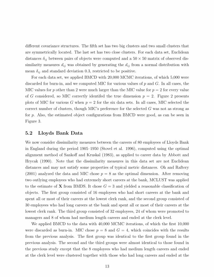
G = 5 and G = 7 as possible optimal numbers of groups.
We applied BMCD with p = 2, 3 for visualization and parsimony. Values of MIC are given
in Table 2. When p = 2, MIC chooses G = 7 and when p = 3 it chooses G = 8, but MIC
has about the same value at G = 5 and G = 7. Figure 8(a) presents the two-dimensional
object configuration from BMCD with the actual five known phases. There are significant
overlaps between the actual clusters. Figure 8(b) shows the estimated object configuraton
and classification results from BMCD with p = 2 and G = 5. It can be seen that BMCD
yields a reasonable clustering of the objects.
We compared the clustering results for p = 2, p = 3, and p = 16, when G = 5. There are
20 mismatches between p = 2 and p = 16, and 22 mismatches between p = 3 and p = 16.
Thus, the proportion of mismatches is less than 6% between the low dimensional clustering
and the clustering with the true dimension. Many of the mismatched genes show significant
clustering uncertainties in low dimensions, suggesting that the assessment of uncertainty is
accurate in these cases. We next computed the proportion of mismatches between clustering
from BMCD and the actual five clusters. These are 0.268, 0.266 and 0.279 for p = 16, p = 3,
and p = 2, respectively, indicating that there is almost no difference in clustering quality
between the different dimensions.
As for the Leukemia data, we performed the two-stage scheme of MDS plus model-based
clustering with p = 2 and G = 5, and compared its membership probabilities with those
20

from BMCD. The main conceptual difference between the two methods lies in whether X
is fixed or randomly generated at each MCMC iteration. In almost all cases the two-stage
scheme provides more extreme membership probabilities, resulting in a smaller posterior
standard deviation. This again suggests that first estimating object configuration and then
clustering (as opposed to doing both simultaneously as in BMCD) does not take into account
the variation in object configuration when clustering and that it may underestimate the
clustering uncertainties.
6 Discussion
We have proposed a model-based clustering method for the situation where the data consist
of dissimilarity measures between pairs of objects. It is also useful for clustering objects in
low dimensional space for visual display and parsimony even when the object coordinates
are given, but are high-dimensional.
Hierarchical models are used to represent the possible sources of error, namely measure-
ment errors in the dissimilarities, errors in estimating object configuration, and errors in
clustering the objects. A probabilistic model is used for the observed dissimilarities and a
mixture model is used for the unobserved latent object configuration. The object configu-
ration, the mixture model parameters, and the objects’ group memberships are estimated
simultaneously via Bayesian inference using MCMC. The object configuration can be used
for display of objects and the mixture parameters can be used for clustering objects. Thus,
the method performs MDS and model-based clustering simultaneously, taking account of the
errors simultaneously rather than sequentially and hence yielding a reasonable measure of
clustering uncertainty.
In contrast, other methods of clustering from dissimilarity measures either do not incorpo-
rate all the errors or do not take them into account simultaneously. In Table 3 we summarize
some possible alternative types of technique for clustering using dissimilarity data. The first
consists of heuristic clustering methods which can cluster directly from dissimilarities, such
as hierarchical agglomerative clustering, k means, and self-organizing maps. The second
scheme is a sequential application of a typical MDS, which gives object configuration with-
out estimation error, and model-based clustering, which provides clustering uncertainty. The
third scheme is a sequential application of BMDS, which provides object configuration as
well as estimation error, and model-based clustering.
When the estimated dimension is high, we have compared BMDS with the selected di-
21
(a) Five known classesdim 1
dim
2
-4 -2 0 2 4
-4-2
02
4
1 1
1
1
1 1
1 1
1
1
1
1
11
11
11
111
1 1 11
1
1
11
1
1
1
1
1 1
1
1
1
111
1
1
1
1
11
1
1
1
1
1
1
11
1
1 1
11
1
11
111
1
22
2
2 2
2
2
2
2
22
22
2
2
2
22
2
2
22
2
2
2
222
22
22
2
2
2
2
2
2
2
2
2
2 2
2
2
2
2
2
22
2
2
2
2
2
2
2
2
22
2
2
2
22
22
22
22
2
2
22
2
2
2 22
2
2
2
2
22
2
2
2
2
2
22
2
2 2
2
222
2
2
2
2
2
2
2
2
2
2
2
2
22
2
22
2
2
22
2
2
2
2
22
22
2 2
2
2 22
3
33
33
3 33
33
3
3
3
3
3
3 3
3
3
33
3
3
3
3
3
3
3
33 3
3
3
3
3
3
3
3
33
3
33
3
33
33
3
3
3
3
33
333
333
3
3
3
3
3
33
3
3
3
3
3
3
3
3
4
4
4
4
4
4
4
44
4
44
4
4
4
4
4
4
4
4
4
4
4
4
4 44 4
44
4
4
4
4
4
4
4
4
4
4
4
44
4
4
4 44
4
4
44
55
5
5
5
5
5
55
555
5
5
5
5
5
5
55
5
5
5
5
5
55
5
5
5
5
555
5
5
5
5
5
5
5
555 5
5
5
5
55
55
5
5
5
(b) Classification from BMCDdim 1
dim
2
-4 -2 0 2 4
-4-2
02
4
1 1
2
5
1 1
5 5
5
5
1
2
11
11
11
111
1 1 11
1
1
11
2
2
5
2
1 1
1
1
1
111
5
5
1
5
11
1
1
1
1
1
1
11
5
1 1
51
1
11
215
5
22
2
2 2
2
2
2
2
22
22
2
2
2
22
2
2
22
1
2
2
222
22
22
2
2
2
2
2
2
2
2
2
2 2
2
2
2
2
2
22
2
2
1
2
2
2
2
3
11
2
1
3
22
11
22
22
2
3
22
2
2
2 22
1
2
2
2
22
2
2
2
2
2
22
2
2 2
2
222
2
2
2
2
2
2
2
2
1
2
1
2
11
2
22
2
2
11
1
1
1
2
22
22
2 2
1
2 22
3
33
33
3 33
24
2
3
2
2
3
3 3
4
2
22
4
4
2
4
3
2
2
33 2
3
3
2
1
3
4
1
34
2
22
2
33
33
2
2
3
3
44
334
334
2
2
2
3
2
42
3
2
2
2
2
1
3
2
4
5
4
3
5
3
4
44
5
34
5
5
4
5
4
3
4
5
3
4
4
4
4 44 4
44
4
3
4
5
4
4
4
4
5
5
5
44
4
5
4 43
3
3
44
55
1
5
5
5
5
55
555
4
5
5
5
5
5
55
5
5
5
5
5
55
5
5
4
5
555
5
5
5
5
5
5
5
555 5
5
5
5
55
55
5
5
5
Figure 8: Scatterplots of object configuration from BMCD with p = 2 in Yeast data andtheir classifications: (a) presents the actual five clusters and (b) presents the classificationfrom BMCD with G = 5.
22

Table 3: Three Sources of Errors in Clustering with Dissimilarities
HeuristicError Sources clustering MDS+ MBC BMDS + MBC BMCDDissimilarity no no yes yes
Object configuration not applicable no yes yesClustering no yes yes yes
Simultaneous consideration no no no yes
mension with BMDS with low dimension (2 or 3). We found that the clustering results were
very similar, and that those misclassified in the low-dimensional analysis had high cluster-
ing uncertainties, which is good. Thus, in practice BMDS low dimensional configurations
may be good enough for many purposes, especially if it is followed up with more intensive
investigation of objects with high clustering uncertainty.
We have proposed a Bayesian criterion, MIC, for simultaneously selecting the object
dimension and the number of clusters, which is easy to compute from MCMC output. In
our simulations and in real examples, it worked reasonably well in all cases. MIC varied
more between dimensions than between numbers of clusters, and the choice of dimension
was not affected by the choice of the number of clusters. Thus, as an approximation we
suggest selecting the dimension assuming one cluster (i.e. using BMDS), and then choosing
the number of clusters given the selected dimension. This greatly reduces computation time.
One important area where data come in the form of measures on pairs of objects is social
networks, where data consist of the presence or absence (or in some cases the intensity)
of ties between actors. Hoff, Raftery and Handcock (2002) used ideas similar to those of
Oh and Raftery (2001) to represent actors in a social network by positions in a Euclidean
latent space and estimate the positions. The model used was the same as that of Oh and
Raftery (2001), except that the conditional distribution of “dissimilarities” (in the social
network case, presence or absence of ties) given distances was taken to be binary with a
conditional probability specified by logistic regression, rather than truncated normal. The
analysis of social network data is often motivated by questions about the presence and
nature of clusters in the network, and these are often answered fairly heuristically. It would
seem straightforward to extend the present approach to social network data, again modeling
presence or absence of ties as conditionally binary with a probability depending on distance
in a logistic regression manner. This could provide a more formal way of answering questions
23

about clustering in social networks.
References
[1] Abbott, A. and Hrycak, A. (1990), “Measuring Sequence Resemblance,” American Jour-
nal of Sociology, 96, 144–185.
[2] Banfield, J.D. and Raftery, A.E. (1993). “Model-Based Gaussian and Non-GaussianClustering,” Biometrics, 49, 803–821.
[3] Bishop, C. (1995), Neural Networks for Pattern Recognition, Oxford University Press,Oxford.
[4] Borg, I. and Groenen, P. (1997). Modern Multidimensional Scaling, Springer-Verlag,New York, Berlin.
[5] Buttenfield, B. and Reitsma, R.F. (2002), “Loglinear and Multidimensional ScalingModels of Digital Library Navigation”, Internation Journal of Human-Computer Stud-
ies, 57, 101-119.
[6] Celeux, G., Hurn, M., and Robert C.P. (2000) “Computational and Inferential Difficul-ties with Mixture Posterior Distribution”, Journal of the American Statistical Associa-
tion, 95, 957-970.
[7] Cho, R.J., Campbell, M.J., Winzeler, E.A., Steinmetz, L., Conway, A., Wodicka, L.,Wolfsberg, T.G., Gabrielian, A.E., Landsman, D.J., Lockhart, D.J., and Davis, R.W.(1998), “A Genome-wide Transcriptional Analysis of the Mitotic Cell Cycle”, Molecular
Cell, 2, 65-73.
[8] Condon, E., Golden, B., Lele, S., Raghavan, S., and Wasil, E. (2002), “A VisualizationModel Based on Adjacency Data”, Decision Support Systems, 33, 349-362.
[9] Courrieu, P. (2001), “Two Methods for Encoding Clusters”, Neural Networks, 14, 175-183.
[10] Elvevag, B. and Storms, G. (2002), “Scaling and Clustering in the Study of SemanticDisruptions in Patients with Schizophrenia: a Re-evaluation”, Schizophrenia Research,in press.
[11] Fraley, C. and Raftery, A.E. (1999), “MCLUST: Software for Model-based Cluster Anal-ysis”, Journal of Classification, 16, 297-306.
[12] Fraley, C. and Raftery, A.E. (2002), “Model-Based Clustering, Discriminant Analysis,and Density Estimation”, Journal of the American Statistical Association, 97, 611–631.
[13] Getz, G., Levine, E., and Domany, E. (2000), “Coupled Two-way Clutering Analysis ofGene Microarray Data”, Proceedings of National Academy of Sciences, 97, 12079-12084.
24

[14] Golub, T.R., Slonim, D.K., Tamayo, P., Huard, C., Gaasenbeek, M., Mesirov, J.P.,Coller, M.L., Loh, M.L., Downing, J.R., Caligiuri, M.A., Bloomfield, C.D., and Lander,E.S. (1999), “Molecular Classification of Cancer: Class Discovery and Class Predictionby Gene Expression Monitoring”, Science, 286, 531-537.
[15] Hastings, W.K. (1970), “Monte Carlo Sampling Methods Using Markov Chains andTheir Applications”, Biometrika, 57, 97-109.
[16] Hedenfalk, I.A., Ringer, M., Trent, J., Borg, A. (2002). “Gene Expression in InheritedBreast”, Cancer Research, 84, 1-34.
[17] Hoff, P., Raftery, A.E. and Handcock, M. (2002), “Latent Space Approaches to SocialNetwork Analysis,” Journal of the American Statistical Association, 97, 1090–1098.
[18] Kohonen, T. (2001), Self-Organizing Maps, Springer-Verlag, New York.
[19] MacQueen, J. (1967), “Some Methods for Classification and Analysis of MultivariateObservations,” in Proceedings of the 5th Berkeley Symposium on Mathematical Statistics
and Probability, Vol. 1, eds. L.M.LeCam and J. Neyman, Berkeley, Calif.: University ofCalifornia Press, pp. 281–297.
[20] McLachlan G., and Peel, D. (2000), Finite Mixture Models, Wiley, New York.
[21] Nikkila, J., Toronen, P., Kaski, S., Venna, J., Castren, E., and Wong, G. (2002), “Anal-ysis and Visualization of Gene Expression Data Using Self-Organizing Maps, Neural
Networks, 15, 953-966.
[22] Oh, M-S. (1999), “Estimation of Posterior Density Functions from a Posterior Sample”,Computational Statistics & Data Analysis, 29, 411-427.
[23] Oh, M-S. and Raftery, A. (2001), “Bayesian Multidimensional Scaling and Choice ofDimension”, Journal of the American Statistical Association, 28, 259-271.
[24] Priem, R.L., Love, L., and Shaffer, M.A. (2002), “Executives’ Perceptions of UncertaintySources: A Numerical Taxonomy and Underlying Dimensions”, Journal of Management,28, 725-746.
[25] Ren, S. and Frymier, P.D. (2003), “Use of Multidimensional Scaling in the Selection ofWastewater Toxicity Test Battery Components”, Water Research, 37, 1655-1661.
[26] Sankoff, D. and Kruskal, J.B. (1983), Time Warps, String Edits and Macromolecules,
Reading, Mass.: Addison-Wesley.
[27] Schutze, H. and C. Silverstein (1997), “Projections for Efficient Document Clustering”,ACM SIGIR 97, 74-81.
[28] Sneath, P.H.A. (1957), “The Application of Computers to Taxonomy,” Journal of Gen-
eral Microbiology, 17, 201–206.
25

[29] Sokal, R.R. and Michener, C.D. (1958), “A Statistical Method for Evaluating SystematicRelationships,” University of Kansas Scientific Bulletin, 38, 1409–1438.
[30] Stephens, M. (2000). “Dealing with Label-Switching in Mixture Models,” Journal of the
Royal Statistical Society, Series B, 62, 795–809.
[31] Stovel, K., Savage, M., and Bearman, P. (1996), “Ascription into Achievement: Modelsof Career Systems at Lloyds Bank, 1890-1970”, American Journal of Sociology, 102,358-399.
[32] Tibshirani, R., Lazzeroni, L., Hastie, T., Olshen, A., and Cox, D. (1999), “The GlobalPairwise Approach to Radiation Hybrid Mapping”, Technical Report, Department ofStatistics, Stanford University.
[33] Welchew, D.E., Honey, G.D., Sharma, T., Robins, T.W., and Bullmore, E.T. (2002),“Multidimensional Scaling of Integrated Neurocognitive Function and Schizophrenia asa Disconnexion Disorder”, NeuroImage, 17, 1227-1239.
[34] Yeung, K., Fraley, C., Murua, A., Raftery, A.E., and Ruzzo, W.L. (2001), “Model-based Clustering and Data Transformation for Gene Expression Data”, Bioinformatics,17, 977-987.
[35] Yin, H. (2002), “Data Visualization and Manifold Mapping Using the ViSOM”, Neural
Networks, 15, 1005-1016.
[36] Young, F.W. (1987), Multidimensional scaling, History, Theory, and Applications, ,edited by Hammer, R.M., Lawrence Erlbaum Associates, Publishers, Hillsdale, NewJersey.
26

APPENDIX
A. Procrustean transformation
• Step 0: Let J be the centering matrix, i.e., J = I − 1/n11′, where I is the identitymatrix and 1 is the vector of all 1’s.
• Step 1: Compute C = X∗′JX.
• Step 2: Compute the singular value decomposition of C, i.e., C = PDQ′, where P andQ are orthogonal matrices and D is a diagonal matrix.
• Step 3: Let T = QP ′.
• Step 4: Let t = 1/n(X∗ − XT)′1.
• Step 5: Transform X by X = XT + 1t′.
B. Relabeling Procedure
Let θ be a d dimensional vector of all the parameters in the mixture distribution, and Jbe the number of components in the mixture.
• Step 0. Estimate elements of θ and their variances using samples taken before the firstlabel switching. Let θ
0 and s0 be the above estimates. Permute the labeling of thelatent classes and deduce θ
1, .., θJ !−1 and s1, .., sJ !−1.
• Step 1. For each sample of θ, do :
(1) Get l∗ which minimizes the squared-distances
||θ − θl||2 =
d∑
i=1
(θi − θli)
2
si
,
for l = 0, ..., J ! − 1, where θi and si are the i−th coordinate of θ and s, respectively.Allocate θ to the label given by l∗. Switch permutations l∗ and 0.
(2) Update θ0 and s0 and derive θ
1, .., θJ !−1 and s1, .., sJ !−1 by permutation.
27