Model-based and model-free learning strategies for wet clutch control

Abhishek Dutta*a, Yu Zhonga, Bruno Depraetereb, Kevin Van Vaerenberghd, Clara Ionescua, Bart Wynsa, Gregory Pinteb, AnnNowed, Jan Sweversc, Robin De Keysera

aElectrical Energy, Systems and Automation, Ghent University, Sint-Pietersnieuwst. 41 Block B2, 9000 Gent, BelgiumCorresponding author* email: Dutta.Abhishek@UGent.be

bFlanders’ Mechatronics Technology Center, Celestijnenlaan 300D, Leuven 3001, BelgiumcDepartment of Mechanical Engineering, Celestijnenlaan 300D, Leuven 3001, Belgium

dAI Lab, Vrije Universiteit Brussel, Pleinlaan 2, B-1050 Brussels, Belgium

Abstract

This paper presents an overview of model-based (Nonlinear Model Predictive Control, Iterative Learning Control and IterativeOptimization) and model-free (Genetic-based Machine Learning and Reinforcement Learning) learning strategies for the controlof wet-clutches. The benefits and drawbacks of the different methodologies are discussed, and illustrated by an experimentalvalidation on a test bench containing wet-clutches. In general, all strategies yield a good engagement quality once they converge.The model-based strategies seems most suited for an online application, because they are inherently more robust and require ashorter convergence time. The model-free strategies meanwhile seem most suited to offline calibration procedures for complexsystems where heuristic tuning rules no longer suffice.

Keywords: nonlinear predictive control, iterative learning control, genetic algorithm, reinforcement learning, hydraulic clutchtransmission

1. Introduction

Wet clutches are commonly used in automatic transmissionsfor off-highway vehicles and agricultural machines to transfertorque from the engine to the load. By disengaging one clutchand engaging another, different transmission ratios can be re-alized. When a clutch engagement is requested, an operatorexpects a fast response without vibrations. The torque trans-fer should thus begin as soon as possible without introducingtorque discontinuities and peaks. These machines are operatedthrough several years and under varying environmental con-ditions such that clutches undergo significant amount of wearand tear, thereby making the clutch control a challenging in-dustrial problem [1]. Contrary to wet-clutches, modeling andcontrol of dry-clutches has received considerable attention inresearch, often considering a stick-slip hybrid model for anal-ysis. A slip control using linear quadratic regulator with forceon clutch piston as input is developed in [2]. While [3] con-cluded that an online MPC scheme for clutch control is notpractically implementable due to the high computation costs,an explicit Model Predictive Control is derived in [4], using alinear cost function for slip control, amongst others. The rep-resentative work on wet-clutch includes optimal control of au-tomotive transmission clutch filling [5], PID control for a wetplate clutch actuated by a pressure reducing valve [6], predic-tive control of a two stage actuation system using piezoelectricactuators for controllable industrial clutches [7], predictive con-trol of an electro-hydraulic actuated wet-clutch for automatictransmission [8] and fast and smooth clutch engagement con-trol for dual-clutch transmissions [9].

The two main challenges for wet clutch control are (i) the in-trinsic complex, non-linear behavior [10], and (ii) the variationof these dynamics over time due to changes in load, oil temper-ature and wear [11]. When similar or repetitive operations haveto be carried out, e.g. the successive engagements of a clutch,learning can be introduced to address these issues. By grad-ually improving the performance with respect to the previoustrial, the complex system behavior can be learned at the cost ofa convergence period, and it also becomes possible to automat-ically adapt to variations in the system’s behaviour or operatingconditions.

In this paper, the potential of several model-based (Non-linear Model Predictive Control (NMPC), Iterative LearningControl (ILC) and Iterative Optimization(IO)) and model-free(Genetic-based Machine Learning (GA) and ReinforcementLearning(RL)) learning strategies are analyzed for the controlof a wet clutch engagement. The model-based approaches relyon a model of the clutch dynamics to update the control sig-nals at each engagement, while in contrast, the model-free onesomit this model and directly explore the input space of possibleclutch control signals using a guided trial-and-error procedure,attempting to maximize the reward/fitness.

The remaining content of this paper is laid out as follows.Section 2 briefly describes the wet-clutch dynamics and objec-tives. Sections 3 and 4 introduce the model-based and model-free learning techniques respectively, and illustrate their appli-cation to wet clutch control. Section 5 details the experimentalresults followed by a comparison of their benefits and draw-backs in section 6. Section 7 finally concludes the paper.

Preprint submitted to Mechatronics March 25, 2014

2. The Wet-clutch

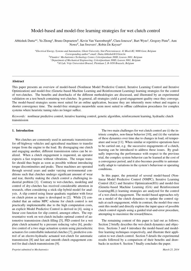
A wet clutch is a device which is used to transmit torque fromone shaft to another by means of friction force. As illustratedin Fig. 1, it contains two sets of friction plates, one that canslide in grooves on the inside of the drum, and another that canslide in grooves on the outgoing shaft. Torque can be trans-ferred between the shafts by pressing both sets together with ahydraulic piston, which can be realized by sending an appro-priate control signal to the servovalve in the line to the clutch.Initially, during the filling phase, the clutch chamber fills upwith oil and the pressure builds up, until it is high enough tocompress the return spring and accelerate the piston. When thepiston advances far enough and presses the plates together, thefilling phase ends and the slip phase begins. During the slipphase, torque is transferred, so that the difference in the angularspeeds between the shafts starts to change. This difference inangular speeds is called the slip speed, and will be shortenedto slip in the remainder. This slip decreases until both shaftshave the same rotation speed. A dynamic model of a hydraulicmulti-plate clutch actuator controlled by an electro valve withinternal pressure feedback [12] or a model based on power ori-ented graphs [13] have been reported in literature. However,it has been argued that, it is frequently unfeasible to transferthese models to other applications because of major modifica-tions that would be needed [8]. Building on this argument, thework in this paper either uses simple system identified modelsor model free control approaches.

Input shaft Output shaftTo valve

Piston

Drum

Friction plates

Return springChamber

Figure 1: Schematic overview of a wet-clutch and its main components.

So far, the goals for the control were not strictly defined. Ingeneral, we want both a fast and smooth engagement. As ameasure for this smoothness, we use the highest absolute valueof the second derivative of the slip (the jerk), since it is stronglyrelated to the experienced operator comfort [14]. For a givenengagement duration, we then want to find the control yieldingthe lowest absolute value of jerk. This can be realized by a shortfilling phase (without torque transfer) followed by a smoothtransition into the slip phase (buildup of torque), after whichthe load has to be synchronized further, still in a smooth man-ner (significant torque transfer).

To validate the developments an experimental setup is used,where an electromotor (30 kW) drives a flywheel (2.5 kgm2) viaa torque converter and two mechanical transmissions, as shownin Fig. 2. The controllers are applied to the first range clutch ofthe left transmission while the right transmission is used onlyto vary the load observed by the first transmission and to ap-ply an adjustable braking torque. The controlled transmissionis equipped with sensors measuring the speeds of the different

Electromotor

Controlled transmission Load transmission

Flywheel

Motor

Torque converter

Clutch

Ratioselector

Flywheel

Brake

Figure 2: Experimental setup with wet clutches.

shafts and the pressure of the oil in the line to the clutches.An additional torque sensor is installed to illustrate the perfor-mance, but it is not used for the control itself. All experimentsare performed with a fixed engine speed, while the output startsat standstill and is then accelerated by engaging the clutch forfirst gear in the controlled transmission. The initial conditionsare zero current and atmospheric pressure. A dSPACE 1103board is used to control the setup. The entire wet-clutch dy-namics is subjected to the following physical constraints:

0 ≤ Current (Amps) ≤ 0.8 (1)0 ≤ Pressure (Bars) ≤ 140 ≤ S lip (normalized) ≤ 1

Clearly, the outlined goals are qualitative and therefore torealize them as parametric trajectories, an element of learningis necessary for the control of wet-clutches. This motivates usto integrate learning in model-based controllers or to developcompletely model-free learning strategies.

3. Model-Based Learning Control

This section discusses three model-based learning techniquesfor wet clutch control. A two-level learning control schemebased on NMPC is presented first, followed by a similar two-level control scheme using ILC instead of MPC. Afterwards,the IO technique is presented as an alternative.

3.1. Two-level NMPC (2l-NMPC)

For the wet clutch with its nonlinear transitions between twophases, it is difficult to develop a single performant control al-gorithm. We therefore propose to use separate controllers for

2

Nonlinear model Nonlinear model

Optimization

yes

no

Process

Impulse input

|U |!!Ubase=Ubase+U

R Y G

Ubase

u(t|t)=ubase(t|t)+"u(t|t)

y(t)

Figure 3: NEPSAC algorithm flowchart, where R, Y ,G,Ubase are the referencebase output, step response matrix, base input and u, δu, y are the input, incre-ment and output respectively.

each phase. This simplifies the control design, but also the iden-tification, since a model for each phase separately is sufficientinstead of a global model. To further reduce the complexity,we only consider tracking controllers. For the clutch, we thenhave a first controller aiming to track a pressure reference inthe filling phase, which is deactivated once the slip phase be-gins, at which point a second controller is activated to track aslip reference.

MPC is a form of control in which the current control actionis obtained by solving on-line, during each sampling period,a finite horizon open-loop optimal control problem taking intoaccount the various constraints on the system [15]. Over thelast three decades MPC has occupied the center stage in thecontrol research community and had a tremendous impact onthe advances in process industry as well [16].

The (Nonlinear) Extended Prediction Self-Adaptive Controli.e. (N)EPSAC [17], (N)MPC principle is depicted in Fig. 3.The process is modeled as in [18]:

y(t) = x(t) + n(t) (2)

with y(t), x(t), n(t) as process output, model output, pro-cess/model disturbance respectively. The fundamental step isbased on the output prediction using the process model givenby:

y(t + k|t) = x(t + k|t) + n(t + k|t) (3)

where y(t + k|t) is the prediction of process output after k sam-ples made at time instant t, over the prediction horizon fromN1 to N2, based on prior measurements and postulated valuesof inputs. Prediction of model output x(t + k|t) and of colorednoise process n(t + k|t) can be obtained by the recursion of pro-cess model and filtering techniques, respectively. The futureresponse can be expressed as:

y(t + k|t) = ybase(t + k|t) + yoptimize(t + k|t) (4)

where the two contributing terms have the following origins:

• ybase(t + k|t) is the cumulative effect of past control inputs,the apriori defined future control actions ubase(t + k|t) andthe predicted disturbances. To predict these disturbances,n(t) = C(q−1)/D(q−1).e(t) is used, with e(t) white noise,and the filter C/D is often chosen as an integrator to en-sure zero steady state error and (q−1) is the backward shiftoperator.

• yoptimize(t + k|t) is the effect of the additions δu(t + k|t)that are optimized and added to ubase(t + k|t), accord-ing to δu(t + k|t) = u(t + k|t) − ubase(t + k|t). The ef-fect of these additions is the discrete time convolution of∆U = {δu(t|t), . . . δu(t + Nu − 1|t)} with the impulse re-sponse coefficients of the system (G matrix), where Nu isthe chosen control horizon.

The control ∆U is the solution to the following constrained op-timization problem:

min∆U{V = ΣN2k=N1

[r(t + k|t) − y(t + k|t)]2 + λΣNu−1k=0 [δu(t + k|t)]2}

sub ject to M.∆U ≤ N (5)

where the first term in V aims to achieve a good tracking of thereference r(t + k|t), while the second term aims to reduce thecontrol effort, and the weighting factor λ selecting their relativeimportance. The various input and output constraints can all beexpressed in terms of ∆U, resulting in the matrices M,N andis solved online by active-sets based primal-dual optimization[19].

When a nonlinear system f [.] is used for x(t), the superpo-sition of (4) is valid only if the term yoptimize(t + k|t) is smallenough compared to ybase(t + k|t). This is true when δu(t + k|t)is small, which is the case if ubase(t + k|t) is close to the opti-mal u∗(t + k|t). To address this condition, the idea is to recur-sively compute δu(t + k|t), within the same sampling instant,until δu(t + k|t) converges to 0. Inside the recursion ubase(t + k|t)is updated each time to ubase(t + k|t) + δu(t + k|t). This is illus-trated in Fig. 3, where R, Y ,Ubase are now in the vector form ofthe signals r, ybase, ubase introduced before.

A third-order linear input-output model for the filling phase(from current to pressure) sampled at 1ms and a fourth-orderpolynomial nonlinear state-space (PNLSS) model containingterms in powers of states and input for the slip phase (fromcurrent to slip) sampled at 10ms have been identified [20]. AnMPC controller with N1 = 2,Nu = 1,N2 = 10, λ = 0, C

D =

1/(1 − q−1) is used to obtain a mean-level control in the fillphase. The short control-horizon ensures that the optimizationis tractable within the allowed 1ms sampling time. The NMPCcontroller is designed with parameters N1 = 1,Nu = 4,N2 =

5, λ = O(102),C/D = 1/(1 − q−1) for slip control. The chosencombination of control horizon and control penalty gives thecontroller enough degrees of freedom for tracking and simul-taneously ensures smooth control action. The slower samplingtime of 10ms allows sufficient time for the NEPSAC iterations(less than 5) to converge. The prediction horizons for both thesecontrollers are chosen to ensure feasibility and stability as theyare subjected to polytopic input and output constraints (1).

3

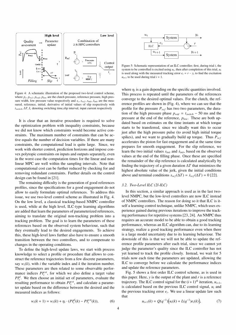
Figure 4: A schematic illustration of the proposed two-level control scheme,where pc, pre f , pwid , plow are the clutch pressure, reference pressure, high pres-sure width, low pressure value respectively and sc, sre f , sinit , sinit are the mea-sured, reference, initial, derivative of initial values of slip respectively withtswitch,∆T, Ic denoting switching time,slip interval, input current respectively

It is clear that an iterative procedure is required to solvethe optimization problem with inequality constraints, becausewe did not know which constraints would become active con-straints. The maximum number of constraints that can be ac-tive equals the number of decision variables. If there are manyconstraints, the computational load is quite large. Since, wework with shorter control, prediction horizons and impose con-vex polytopic constraints on inputs and outputs separately, evenin the worst case the computation times for the linear and non-linear MPC are well within the sampling intervals. Note thatcomputational cost can be further reduced by checking for andremoving redundant constraints. Further details on the controldesign can be found in [21].

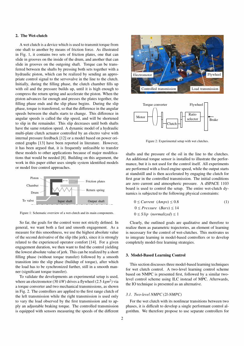
The remaining difficulty is the generation of good referencesprofiles, since the specifications for a good engagement do notallow to easily formulate optimal references. To address thisissue, we use two-level control scheme as illustrated in Fig. 4.On the low level, a classical tracking-based NMPC controlleris used, while at the high level, ILC-type learning algorithmsare added that learn the parameters of parameterized references,aiming to translate the original non-tracking problem into atracking problem. The goal is to learn the parameters of thesereferences based on the observed system behaviour, such thatthey eventually lead to the desired engagements. To achievethis, these high-level laws further also have to ensure a smoothtransition between the two controllers, and to compensate tochanges in the operating conditions.

To define the high-level update laws, we start with processknowledge to select a profile or procedure that allows to con-struct the reference trajectories from a few discrete parameters,say wi(k), with i the variable index and k the iteration number.These parameters are then related to some observable perfor-mance indices PIest

i , for which we also define a target valuePId

i . We then choose an initial set of parameters, evaluate theresulting performance to obtain PIest

i , and calculate a parame-ter update based on the difference between the desired and themeasured indices as follows:

wi(k + 1) = wi(k) + ηi · (PIdi (k) − PIest

i (k)), (6)

System

System

ILC −+

ui yi

ui+1 yi+1

rei

Figure 5: Schematic representation of an ILC controller; first, during trial i, thesystem to be controlled is excited using ui, then after completion of this trial, uiis used along with the measured tracking error ei = r − yi to find the excitationui+1 to be used during trial i + 1.

where ηi is a gain depending on the specific quantities involved.This process is repeated until the parameters of the referencesconverge to the desired optimal values. For the clutch, the ref-erence profiles are shown in (Fig. 4), where we can see that theprofile for the pressure Pre f has two two parameters, the dura-tion of the high pressure phase pwid = tswitch − 50 ms and thepressure at the end of the reference, plow. These are both up-dated based on estimates on the time instants at which torquestarts to be transferred, since we ideally want this to occurjust after the high pressure pulse (to avoid high initial torquespikes), and we want to gradually build up torque. Thus Pre f

accelerates the piston for fast engagement and at the same timeprepares for smooth engagement. For the slip reference, welearn the two initial values sinit and sinit, based on the observedvalues at the end of the filling phase. Once these are specifiedthe remainder of the slip reference is calculated analytically byfinding the trajectory of a given duration ∆T that minimizes thehighest absolute value of the jerk, given the initial conditionsabove and terminal conditions sre f (∆T ) = sre f (∆T ) = 0 [22].

3.2. Two-Level ILC (2l-ILC)

In this section, a similar approach is used as in the last two-level NMPC, but the low-level controllers are now ILC insteadof NMPC controllers. The reason for doing so it that ILC is it-self a learning control technique, unlike NMPC, which uses ex-perience gained during previous iterations to improve the track-ing performance for repetitive systems [23, 24]. An NMPC thusrequires an accurate model to be able to obtain a good trackingperformance, whereas an ILC algorithm can, due to its learningstrategy, realize a good tracking performance even when thereis a large model uncertainty due to its learning behaviour. Thedownside of this is that we will not be able to update the ref-erence profile parameters after each trial, since we cannot yetjudge the parameter’s quality since the ILC controller has notyet learned to track the profile closely. Instead, we wait for 5trials now each time the parameters are updated, allowing theILC to converge before we calculate the performance indicesand update the reference parameters.

Fig. 5 shows a first order ILC control scheme, as is used inthis paper. Here, y is the output of the plant and r is a referencetrajectory. The ILC control signal for the (i+1)th iteration, ui+1,is calculated based on the previous ILC control signal, ui andthe previous tracking error ei. We use a linear update law suchthat

ui+1(k) = Q(q−1)(ui(k) + L(q−1)ei(k)

), (7)

4

with linear operators Q and L that can be chosen during thedesign of the ILC controller. For this update law, a convenientfrequency domain criterion for monotonic convergence can bederived [23, 24]. For a plant with FRF P(ω), a monotonicallydecreasing tracking error is obtained with controller (7) if

|Q( jω)(1 − L( jω)P( jω)

)| < 1, (8)

with Q( jω) and L( jω) the frf’s of the operators Q and L. Itis also possible to derive an expression for the remaining errorafter convergence, E∞( jω), which becomes

E∞( jω) =1 − Q( jω)

1 − Q( jω)(1 − L( jω)P( jω)

)R( jω), (9)

where R(ω) is the Fourier transform of the reference r.Based on these expressions, [23] and [24] show that by se-

lecting L( jω) = P( jω)−1 and Q( jω) = 1, perfect tracking wouldbe obtained after only one iteration. However when there is un-certainty about P( jω), this choice of L( jω) becomes impossi-ble. It is then needed to select an estimate P( jω) of the plantand use L( jω) = αP( jω)−1 with 0 < α < 1. This way, therobustness increases while the learning slows down, but a goodperformance is still achieved. This is possible for all frequen-cies where the angular deviation between the system and thenominal model does not exceed 90◦. Once this deviation be-comes larger, the value of |Q( jω)| has to be decreased in orderto satisfy (8). It then follows from (9) that perfect tracking canno longer be achieved, not even by learning more slowly. As theuncertainty typically increases with the frequency, Q( jω) is of-ten chosen as a low pass filter, effectively deactivating the ILCcontroller for high frequencies with much uncertainty, whileobtaining good tracking in the less uncertain, lower frequencyrange.

Since an accurate plant model is not required to achieve agood tracking performance, ILC is well suited to the controlof wet-clutch engagements, where the plant dynamics are non-linear and vary significantly over time. For each of the two ILCcontrollers, a single, linearized model, approximating the plantdynamics in all conditions suffices, keeping the required mod-eling effort small. With these choices it becomes possible todesign ILC controllers that achieve bandwidths of > 10 Hz, butin practise the controllers are detuned intentionally. Especiallyin the slip phase this is needed, as it is preferable to keep thejerk low instead of aggressively tracking the reference.

For ILC the computational cost is very low, since it only re-quires linear filtering operations (Q and L), but to do so it doesrequire storing a number of vectors of a length equal to the du-ration of an engagement (for example the previous tracking er-ror). Implementation on typical industrial controllers is thuspossible, but when this is not the case it is more likely due tomemory problems than due to a high computational load. Amore detailed description of the implementation applied to thewet clutch can be found in [25].

3.3. Iterative OptimizationAnother technique based on learning control, denoted itera-

tive optimization, has been developed as an alternative to the

Control signal optimization

Quality assessment

Recursive identification Memory

System

High level

Low level

Models

Constraints

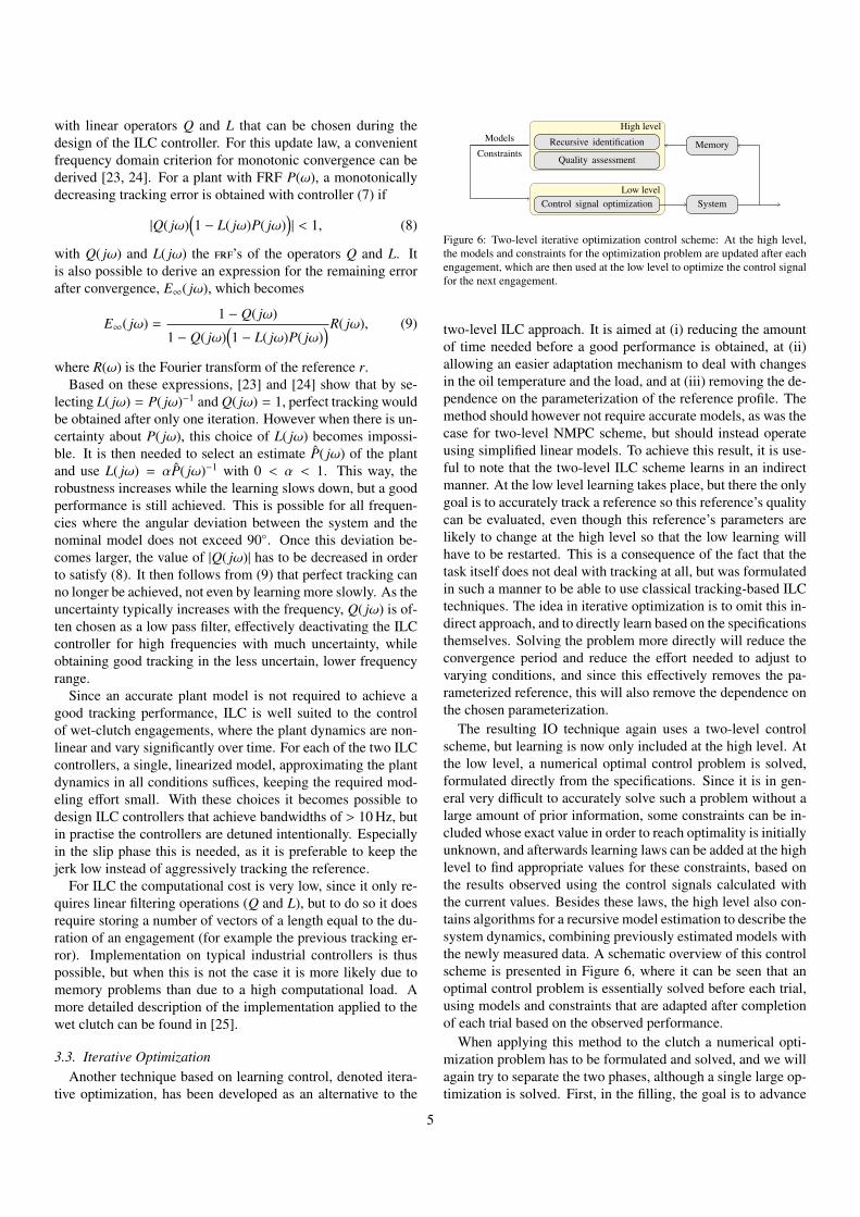
Figure 6: Two-level iterative optimization control scheme: At the high level,the models and constraints for the optimization problem are updated after eachengagement, which are then used at the low level to optimize the control signalfor the next engagement.

two-level ILC approach. It is aimed at (i) reducing the amountof time needed before a good performance is obtained, at (ii)allowing an easier adaptation mechanism to deal with changesin the oil temperature and the load, and at (iii) removing the de-pendence on the parameterization of the reference profile. Themethod should however not require accurate models, as was thecase for two-level NMPC scheme, but should instead operateusing simplified linear models. To achieve this result, it is use-ful to note that the two-level ILC scheme learns in an indirectmanner. At the low level learning takes place, but there the onlygoal is to accurately track a reference so this reference’s qualitycan be evaluated, even though this reference’s parameters arelikely to change at the high level so that the low learning willhave to be restarted. This is a consequence of the fact that thetask itself does not deal with tracking at all, but was formulatedin such a manner to be able to use classical tracking-based ILCtechniques. The idea in iterative optimization is to omit this in-direct approach, and to directly learn based on the specificationsthemselves. Solving the problem more directly will reduce theconvergence period and reduce the effort needed to adjust tovarying conditions, and since this effectively removes the pa-rameterized reference, this will also remove the dependence onthe chosen parameterization.

The resulting IO technique again uses a two-level controlscheme, but learning is now only included at the high level. Atthe low level, a numerical optimal control problem is solved,formulated directly from the specifications. Since it is in gen-eral very difficult to accurately solve such a problem without alarge amount of prior information, some constraints can be in-cluded whose exact value in order to reach optimality is initiallyunknown, and afterwards learning laws can be added at the highlevel to find appropriate values for these constraints, based onthe results observed using the control signals calculated withthe current values. Besides these laws, the high level also con-tains algorithms for a recursive model estimation to describe thesystem dynamics, combining previously estimated models withthe newly measured data. A schematic overview of this controlscheme is presented in Figure 6, where it can be seen that anoptimal control problem is essentially solved before each trial,using models and constraints that are adapted after completionof each trial based on the observed performance.

When applying this method to the clutch a numerical opti-mization problem has to be formulated and solved, and we willagain try to separate the two phases, although a single large op-timization is solved. First, in the filling, the goal is to advance

5

into to the slip phase as soon as possible, without causing un-wanted torque spikes that could cause operator discomfort. Af-terwards, once the slip phase begins, the goal becomes to fur-ther engage the clutch while keeping the jerk as low as possi-ble. To optimize the control signals accordingly, a piece-wiselinear model structure is selected, with one model to predict thepressure and piston position in the filling phase and one to pre-dict the pressure and the slip in the slip phase, while recursiveestimation techniques are added to learn these online, so thatthese models are tuned to the observed behaviour. Transitionconstraints are also added to ensure a smooth transition occursbetween both phases, but since the optimal conditions in whichto go from the filling to the slip are unknown, values for theseare chosen and afterwards their optimal values are found usinglearning laws. Using the notation that z(k) denote the discretetime finite difference (z(k + 1) − z(k))/Ts with Ts the samplingtime, the problem to be solved at the low level is then

minu(:),

x(:), p(:), s(:), z(:),jmax,K1,K2

K1 + γ ∗ jmax, (10a)

s.t.

filling phase: k = 1 : K1

x(k + 1) = A1x(k) + B1u(k), (10b) p(k)

z(k)

= C1x(k) + D1u(k), (10c)

umin ≤ u(k) ≤ umax, (10d)pmin ≤ p(k) ≤ pmax, (10e)

slip phase: k = K1 + 1 : K1 + K2

x(k + 1) = A2x(k) + B2u(k), (10f) p(k)

s(k)

= C2x(k) + D2u(k), (10g)

0 ≤ s(k) ≤ strans, (10h)− jmax ≤ s(k) ≤ jmax, (10i)

transition and terminal constraints:x(K1 + 1) = xtrans, (10j)

p(K1) = p1, (10k)z(K1) = zfinal, ˙z(K1) ≤ ε, (10l)

s(K1 + K2) = 0, s(K1 + K + 2) = 0 (10m)

In this problem, the piecewise structure can clearly be seen, asthe problem is split into two parts with K1 and K2 samples foreach phase respectively (with K1 + K2 = T/Ts), and a set ofconstraints which need to be respected during the transition. Inorder for the solutions of this problem to yield good engage-ments, the high-level learning laws recursively identify the ma-trices Ai, Bi, Ci and Di. Since the piston position is not mea-sured, its model z can however not be estimated so easily, sohere we use a simple first principles model and rescale it usinga rule similar to (6). Similar rules are included for xtrans, p1 andzfinal.

In terms of computational load, problem (10) reduces to aconvex optimization problem (either a linear or quadratic pro-gram depending on the regularization), assuming we know theduration of the filling phase. Since in reality we don’t knowthis duration and need to find the optimal one, this problem isnot solved as a single convex problem, but we instead solve itby solving a series of convex sub-problems, each with a differ-ent but fixed filling phase duration, after which we then use theone with the shortest still feasible duration. Since this only re-quires solving a series of convex problems, the total solutionsare found in about 1s on a normal laptop CPU. However, noattempts have been made to further reduce the calculation timesince the problems are solved in between engagements (and notat every timestep), so that the calculation can be spread out overtime. A more detailed description of the implementation can befound in [26].

The control techniques presented so far are based on cer-tain characterization of the system dynamics. In very complexsystems, however, another approach could be to focus entirelyon improving the performance without the intermediate step ofmodeling the system. Two representative techniques which fallin this category are discussed next.

4. Model-free Learning Control

Next to the model-based algorithms described so far in sec-tion 3, the potential of model-free algorithms has also beeninvestigated. To date, most complex mechatronic systems arecontrolled using either a model-based technique, or using con-trollers tuned during an experimental calibration. Even thoughthese latter are often tuned without the use of a model, thistuning is usually done in an ad-hoc manner derived from sys-tem knowledge or insight, and a systematic model-free ma-chine learning (ML) strategy is rarely applied. These strate-gies would however make it possible to also learn controllersfor more complex situations, where insight would not be suffi-cient to yield the desired behavior. This can improve the currentcontrollers by being able to use more complex control laws, orallowing to optimize a cost criterion and taking into accountconstraints. This can further also make it possible to developcontrollers for more complex applications, for which now nogood controllers can be tuned automatically.

Nowadays, wet clutches in industrial transmissions are filledusing a feed forward controller of the current (with a set of tun-able parameters) to the electro-hydraulic valve. These are nowtuned using some heuristic rules, but now we will use model-free learning control methods instead, while still looking foroptimal parameterized control signals.

4.1. Genetic Algorithm

Genetic Algorithm (GA) is a stochastic search algorithm thatmimics the mechanism of natural selection and natural genet-ics, and belong to the larger class of evolutionary algorithms(EA). They are routinely applied to generate useful solutionsfor optimization and search problems, often for complex non-convex problem where gradient-based methods fails to find the

6

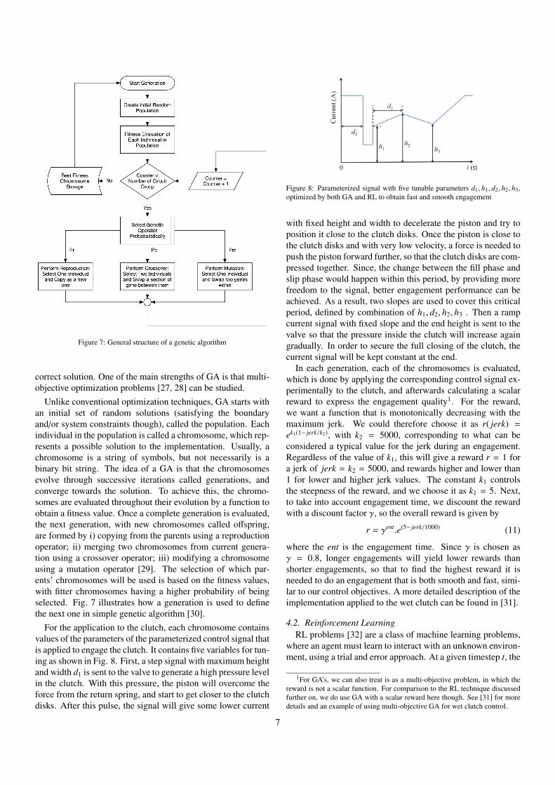
Figure 7: General structure of a genetic algorithm

correct solution. One of the main strengths of GA is that multi-objective optimization problems [27, 28] can be studied.

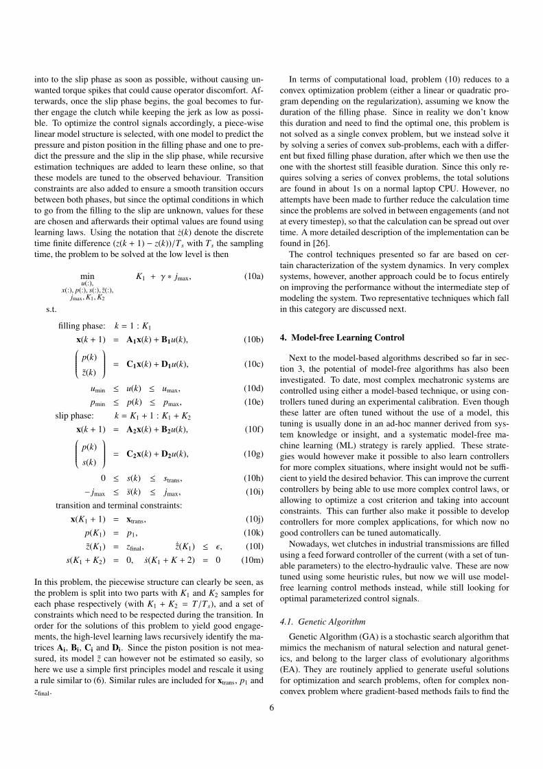
Unlike conventional optimization techniques, GA starts withan initial set of random solutions (satisfying the boundaryand/or system constraints though), called the population. Eachindividual in the population is called a chromosome, which rep-resents a possible solution to the implementation. Usually, achromosome is a string of symbols, but not necessarily is abinary bit string. The idea of a GA is that the chromosomesevolve through successive iterations called generations, andconverge towards the solution. To achieve this, the chromo-somes are evaluated throughout their evolution by a function toobtain a fitness value. Once a complete generation is evaluated,the next generation, with new chromosomes called offspring,are formed by i) copying from the parents using a reproductionoperator; ii) merging two chromosomes from current genera-tion using a crossover operator; iii) modifying a chromosomeusing a mutation operator [29]. The selection of which par-ents’ chromosomes will be used is based on the fitness values,with fitter chromosomes having a higher probability of beingselected. Fig. 7 illustrates how a generation is used to definethe next one in simple genetic algorithm [30].

For the application to the clutch, each chromosome containsvalues of the parameters of the parameterized control signal thatis applied to engage the clutch. It contains five variables for tun-ing as shown in Fig. 8. First, a step signal with maximum heightand width d1 is sent to the valve to generate a high pressure levelin the clutch. With this pressure, the piston will overcome theforce from the return spring, and start to get closer to the clutchdisks. After this pulse, the signal will give some lower current

Figure 8: Parameterized signal with five tunable parameters d1, h1, d2, h2, h3,optimized by both GA and RL to obtain fast and smooth engagement

with fixed height and width to decelerate the piston and try toposition it close to the clutch disks. Once the piston is close tothe clutch disks and with very low velocity, a force is needed topush the piston forward further, so that the clutch disks are com-pressed together. Since, the change between the fill phase andslip phase would happen within this period, by providing morefreedom to the signal, better engagement performance can beachieved. As a result, two slopes are used to cover this criticalperiod, defined by combination of h1, d2, h2, h3 . Then a rampcurrent signal with fixed slope and the end height is sent to thevalve so that the pressure inside the clutch will increase againgradually. In order to secure the full closing of the clutch, thecurrent signal will be kept constant at the end.

In each generation, each of the chromosomes is evaluated,which is done by applying the corresponding control signal ex-perimentally to the clutch, and afterwards calculating a scalarreward to express the engagement quality1. For the reward,we want a function that is monotonically decreasing with themaximum jerk. We could therefore choose it as r( jerk) =

ek1(1− jerk/k2), with k2 = 5000, corresponding to what can beconsidered a typical value for the jerk during an engagement.Regardless of the value of k1, this will give a reward r = 1 fora jerk of jerk = k2 = 5000, and rewards higher and lower than1 for lower and higher jerk values. The constant k1 controlsthe steepness of the reward, and we choose it as k1 = 5. Next,to take into account engagement time, we discount the rewardwith a discount factor γ, so the overall reward is given by

r = γent.e(5− jerk/1000) (11)

where the ent is the engagement time. Since γ is chosen asγ = 0.8, longer engagements will yield lower rewards thanshorter engagements, so that to find the highest reward it isneeded to do an engagement that is both smooth and fast, simi-lar to our control objectives. A more detailed description of theimplementation applied to the wet clutch can be found in [31].

4.2. Reinforcement LearningRL problems [32] are a class of machine learning problems,

where an agent must learn to interact with an unknown environ-ment, using a trial and error approach. At a given timestep t, the

1For GA’s, we can also treat is as a multi-objective problem, in which thereward is not a scalar function. For comparison to the RL technique discussedfurther on, we do use GA with a scalar reward here though. See [31] for moredetails and an example of using multi-objective GA for wet clutch control.

7

agent may execute one of a set of actions, possibly causing theenvironment to change its state and generate a (scalar) reward.Both state and action spaces can be multidimensional, contin-uous or discrete. An agent is represented by a policy, mappingstates to actions. The aim of a RL algorithm is to optimize thepolicy, maximizing the reward accumulated by the agent.

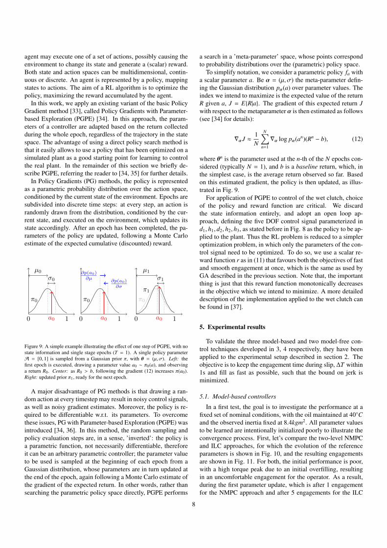
In this work, we apply an existing variant of the basic PolicyGradient method [33], called Policy Gradients with Parameter-based Exploration (PGPE) [34]. In this approach, the param-eters of a controller are adapted based on the return collectedduring the whole epoch, regardless of the trajectory in the statespace. The advantage of using a direct policy search method isthat it easily allows to use a policy that has been optimized on asimulated plant as a good starting point for learning to controlthe real plant. In the remainder of this section we briefly de-scribe PGPE, referring the reader to [34, 35] for further details.

In Policy Gradients (PG) methods, the policy is representedas a parametric probability distribution over the action space,conditioned by the current state of the environment. Epochs aresubdivided into discrete time steps: at every step, an action israndomly drawn from the distribution, conditioned by the cur-rent state, and executed on the environment, which updates itsstate accordingly. After an epoch has been completed, the pa-rameters of the policy are updated, following a Monte Carloestimate of the expected cumulative (discounted) reward.

0 1

π0

a0

µ0

σ0

0 1

π0

a0

∂p(a0)∂µ

∂p(a0)∂σ

0 1

π0

π1

a0

µ1

σ1

Figure 9: A simple example illustrating the effect of one step of PGPE, with nostate information and single stage epochs (T = 1). A single policy parameterA = [0, 1] is sampled from a Gaussian prior π, with θ = (µ, σ). Left: thefirst epoch is executed, drawing a parameter value a0 ∼ π0(a), and observinga return R0. Center: as R0 > b, following the gradient (12) increases π(a0).Right: updated prior π1, ready for the next epoch.

A major disadvantage of PG methods is that drawing a ran-dom action at every timestep may result in noisy control signals,as well as noisy gradient estimates. Moreover, the policy is re-quired to be differentiable w.r.t. its parameters. To overcomethese issues, PG with Parameter-based Exploration (PGPE) wasintroduced [34, 36]. In this method, the random sampling andpolicy evaluation steps are, in a sense, ’inverted’: the policy isa parametric function, not necessarily differentiable, thereforeit can be an arbitrary parametric controller; the parameter valueto be used is sampled at the beginning of each epoch from aGaussian distribution, whose parameters are in turn updated atthe end of the epoch, again following a Monte Carlo estimate ofthe gradient of the expected return. In other words, rather thansearching the parametric policy space directly, PGPE performs

a search in a ’meta-parameter’ space, whose points correspondto probability distributions over the (parametric) policy space.

To simplify notation, we consider a parametric policy fa witha scalar parameter a. Be α = (µ, σ) the meta-parameter defin-ing the Gaussian distribution pα(a) over parameter values. Theindex we intend to maximize is the expected value of the returnR given a, J = E{R|a}. The gradient of this expected return Jwith respect to the metaparameter α is then estimated as follows(see [34] for details):

∇αJ ≈1N

N∑n=1

∇α log pα(an)(Rn − b), (12)

where θn is the parameter used at the n-th of the N epochs con-sidered (typically N = 1), and b is a baseline return, which, inthe simplest case, is the average return observed so far. Basedon this estimated gradient, the policy is then updated, as illus-trated in Fig. 9.

For application of PGPE to control of the wet clutch, choiceof the policy and reward function are critical. We discardthe state information entirely, and adopt an open loop ap-proach, defining the five DOF control signal parameterized ind1, h1, d2, h2, h3, as stated before in Fig. 8 as the policy to be ap-plied to the plant. Thus the RL problem is reduced to a simpleroptimization problem, in which only the parameters of the con-trol signal need to be optimized. To do so, we use a scalar re-ward function r as in (11) that favours both the objectives of fastand smooth engagement at once, which is the same as used byGA described in the previous section. Note that, the importantthing is just that this reward function monotonically decreasesin the objective which we intend to minimize. A more detaileddescription of the implementation applied to the wet clutch canbe found in [37].

5. Experimental results

To validate the three model-based and two model-free con-trol techniques developed in 3, 4 respectively, they have beenapplied to the experimental setup described in section 2. Theobjective is to keep the engagement time during slip, ∆T within1s and fill as fast as possible, such that the bound on jerk isminimized.

5.1. Model-based controllers

In a first test, the goal is to investigate the performance at afixed set of nominal conditions, with the oil maintained at 40◦Cand the observed inertia fixed at 8.4kgm2. All parameter valuesto be learned are intentionally initialized poorly to illustrate theconvergence process. First, let’s compare the two-level NMPCand ILC approaches, for which the evolution of the referenceparameters is shown in Fig. 10, and the resulting engagementsare shown in Fig. 11. For both, the initial performance is poor,with a high torque peak due to an initial overfilling, resultingin an uncomfortable engagement for the operator. As a result,during the first parameter update, which is after 1 engagementfor the NMPC approach and after 5 engagements for the ILC

8

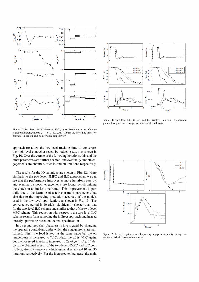
Figure 10: Two-level NMPC (left) and ILC (right): Evolution of the referencesignal parameters, where tswitch, Plow, S init , dS init/dt are the switching time, lowpressure, initial slip and its derivative respectively.

approach (to allow the low-level tracking time to converge),the high-level controller reacts by reducing tswitch as shown inFig. 10. Over the course of the following iterations, this and theother parameters are further adapted, and eventually smooth en-gagements are obtained, after 10 and 30 iterations respectively.

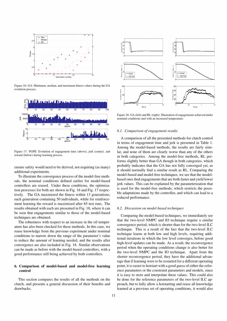
The results for the IO technique are shown in Fig. 12, wheresimilarly to the two-level NMPC and ILC approaches, we cansee that the performance improves as more iterations pass by,and eventually smooth engagements are found, synchronizingthe clutch in a similar timeframe. This improvement is par-tially due to the learning of a few constraint parameters, butalso due to the improving prediction accuracy of the modelsused in the low-level optimization, as shown in Fig. 13. Theconvergence period is 10 trials, significantly shorter than thatfor the two-level ILC scheme and similar to that of the two-levelMPC scheme. This reduction with respect to the two-level ILCscheme results form removing the indirect approach and insteaddirectly optimizing based on the real specifications.

In a second test, the robustness is investigated by changingthe operating conditions under which the engagements are per-formed. First, the load is kept at the same value but the oiltemperature is increased to 70◦C. Next, the oil is 40◦C again,but the observed inertia is increased to 28.6kgm2. Fig. 14 de-picts the obtained results of the two-level NMPC and ILC con-trollers, after convergence, which again takes around 10 and 30iterations respectively. For the increased temperature, the main

Figure 11: Two-level NMPC (left) and ILC (right): Improving engagementquality during convergence period at nominal conditions.

Figure 12: Iterative optimization: Improving engagement quality during con-vergence period at nominal conditions.

9

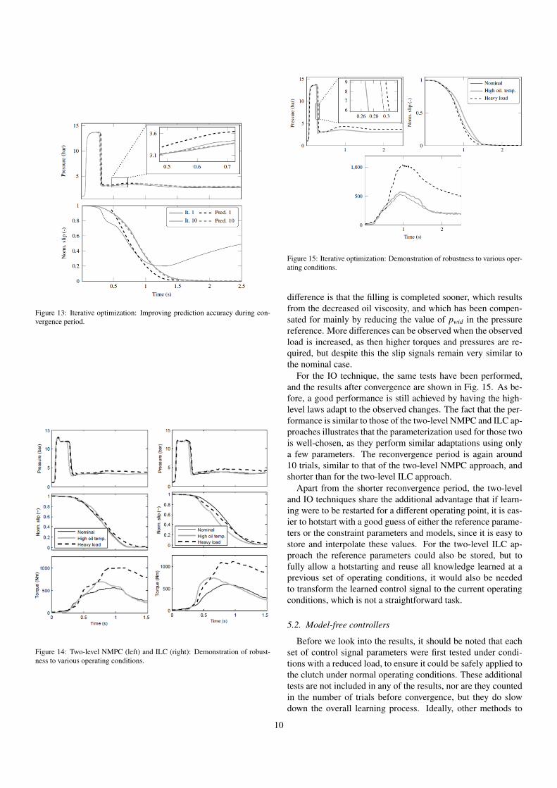
Figure 13: Iterative optimization: Improving prediction accuracy during con-vergence period.

Figure 14: Two-level NMPC (left) and ILC (right): Demonstration of robust-ness to various operating conditions.

Figure 15: Iterative optimization: Demonstration of robustness to various oper-ating conditions.

difference is that the filling is completed sooner, which resultsfrom the decreased oil viscosity, and which has been compen-sated for mainly by reducing the value of pwid in the pressurereference. More differences can be observed when the observedload is increased, as then higher torques and pressures are re-quired, but despite this the slip signals remain very similar tothe nominal case.

For the IO technique, the same tests have been performed,and the results after convergence are shown in Fig. 15. As be-fore, a good performance is still achieved by having the high-level laws adapt to the observed changes. The fact that the per-formance is similar to those of the two-level NMPC and ILC ap-proaches illustrates that the parameterization used for those twois well-chosen, as they perform similar adaptations using onlya few parameters. The reconvergence period is again around10 trials, similar to that of the two-level NMPC approach, andshorter than for the two-level ILC approach.

Apart from the shorter reconvergence period, the two-leveland IO techniques share the additional advantage that if learn-ing were to be restarted for a different operating point, it is eas-ier to hotstart with a good guess of either the reference parame-ters or the constraint parameters and models, since it is easy tostore and interpolate these values. For the two-level ILC ap-proach the reference parameters could also be stored, but tofully allow a hotstarting and reuse all knowledge learned at aprevious set of operating conditions, it would also be neededto transform the learned control signal to the current operatingconditions, which is not a straightforward task.

5.2. Model-free controllers

Before we look into the results, it should be noted that eachset of control signal parameters were first tested under condi-tions with a reduced load, to ensure it could be safely applied tothe clutch under normal operating conditions. These additionaltests are not included in any of the results, nor are they countedin the number of trials before convergence, but they do slowdown the overall learning process. Ideally, other methods to

10

0 5 10 150

0.5

1

1.5

2

2.5

3

Generation number

Fitness

Max

Median

Min

Figure 16: GA: Minimum, median, and maximum fitness values during the GAevolution process.

0 10 20 30 40 50 60 70 80 90 1000

1

2

Eng. tim

e

0 10 20 30 40 50 60 70 80 90 1000

5000

10000

epoch

Jerk

0 10 20 30 40 50 60 70 80 90 1000

5

10

epoch

Retu

rn

Figure 17: PGPE: Evolution of engagement time (above), jerk (center), andreward (below) during learning process.

ensure safety would need to be derived, not requiring (as many)additional experiments.

To illustrate the convergence process of the model-free meth-ods, the nominal conditions defined earlier for model-basedcontrollers are reused. Under these conditions, the optimiza-tion processes for both are shown in Fig. 16 and Fig. 17 respec-tively. The GA maximized the fitness within 13 generations;each generation containing 50 individuals, while for reinforce-ment learning the reward is maximized after 85 test runs. Theresults obtained with each are presented in Fig. 18, where it canbe seen that engagements similar to those of the model-basedtechniques are obtained.

The robustness with respect to an increase in the oil temper-ature has also been checked for these methods. In this case, wereuse knowledge from the previous experiment under nominalconditions to narrow down the range of the parameter’s valueto reduce the amount of learning needed, and the results afterconvergence are also included in Fig. 18. Similar observationscan be made as before with the model-based controllers, with agood performance still being achieved by both controllers.

6. Comparison of model-based and model-free learningcontrol

This section compares the results of all the methods on theclutch, and presents a general discussion of their benefits anddrawbacks.

0

0.2

0.4

0.6

0.8

Current (A

)

0

0.5

1

Norm

. S

lip (

−)

Nominal

High Temp

0 0.5 1 1.50

500

1000

Time (s)

Torque (

Nm

)

0

0.2

0.4

0.6

0.8

Current (A

)

0 0.5 1 1.50

200

400

600

800

Time (s)

Torque (

Nm

)

0

0.5

1

Norm

. S

lip (

−)

Nominal

High Temp

Figure 18: GA (left) and RL (right): Illustration of engagements achieved undernominal conditions and with an increased temperature.

6.1. Comparison of engagement results

A comparison of all the presented methods for clutch controlin terms of engagement time and jerk is presented in Table 1.Among the model-based methods, the results are fairly simi-lar, and none of them are clearly worse than any of the othersin both categories. Among the model-free methods, RL per-forms slightly better than GA though in both categories, whichprobably indicates that the GA has not fully converged yet, asit should normally find a similar result as RL. Comparing themodel-based and model-free techniques, we see that the model-based ones find engagements that are both faster and yield lowerjerk values. This can be explained by the parameterization thatis used for the model-free methods, which restricts the possi-ble adaptations made by the controller, and which can lead to areduced performance.

6.2. Discussion on model-based techniques

Comparing the model-based techniques, we immediately seethat the two-level NMPC and IO technique require a similarconvergence period, which is shorter than for the two-level ILCtechnique. This is a result of the fact that the two-level ILCtechnique learns at both low and high levels, requiring addi-tional iterations in which the low level converges, before goodhigh-level updates can be made. As a result, the reconvergenceperiod when the operating conditions change is also better forthe two-level NMPC and the IO technique. Apart from theshorter reconvergence period, they have the additional advan-tage that if learning were to be restarted for a different operatingpoint, it is easier to hotstart with a good guess of either the refer-ence parameters or the constraint parameters and models, sinceit is easy to store and interpolate these values. This could alsobe done for the reference parameters of the two-level ILC ap-proach, but to fully allow a hotstarting and reuse all knowledgelearned at a previous set of operating conditions, it would also

11

Index 2l-NMPC 2l-ILC IO GA RLAbs(Max(Jerk)) 3.6683 2.8945 3.4133 3.9256 3.618Eng.Time(s) 1.199 1.39 1.277 1.434 1.317

Table 1: An empirical comparison between the model-based and non-model based control techniques based on jerk and engagement times

Method/Property 2l-NMPC 2l-ILC IO GA RLModeling requirement _ ^ ^ ^^ ^^

Learning rate ^^ ^ ^^ __ _

Stability ^ ^ −− −− −−

Learning transient/Safety ^ ^ ^ __ __

Multi-objective ^ ^ ^ ^^ ^

Table 2: Characteristic features of the model-based and model-free techniques

be needed to transform the learned control signal to the currentoperating conditions, which is not a straightforward task.

When comparing the required modeling effort, the two-levelILC technique outperforms the other methods however, as ahighly accurate tracking control can be achieved despite hav-ing a large model uncertainty. In contrast, for NMPC it isneeded to have an accurate non-linear model, which requiresa time-consuming identification. For the IO technique this isnot needed again, but here the performance is limited by thechosen model structure, of which the parameters are afterwardslearnt online.

Even though the ILC approach improves the tracking be-haviour, so that the references can be tracked more accuratelythan with the NMPC approach, it turns out that this may not bebeneficial for the current application, where aggressive controlcan lead to unwanted vibrations and high jerk values.

6.3. Discussion on model-free techniques

Comparing the model-free techniques, we see that with thesame reward/fitness function, both methods manage to yieldsimilar engagements, but RL converges faster than GA.

The type of reward/fitness that was used is the same for both,and is a trade-off between the jerk and the engagement duration.These can be combined into a single scalar reward, which isthe way in which RL typically operates. For GA it is howeveralso possible not to use a fixed trade-off, but to really treat itas multiple objectives without extra cost, and find a completepareto-front.

6.4. Comparison of model-based and model-free techniques

Model-based methods have a few advantages over model-free methods. First of all, they allow more freedom in the de-termination of the shape of the control signals. They will there-fore generally be able to find the optimal solution, whereas forthe model-free methods this is only possible if the chosen pa-rameterization allows this. The convergence period is also sig-nificantly shorter for model-based methods, and hotstarting isoften possible, which makes them more applicable for onlineadaptive purposes. Another advantage is that they posses an in-herent robustness to parameter uncertainties due to the abilityto use feedback. They finally also make it easier to predict the

behaviour and thus ensure safety, even during the convergenceperiod.

Despite these advantages of model-based methods, model-free methods also have some attractive properties for the con-trol of mechatronic systems. Their main benefit is that theycan operate without model, and thus require no identificationor apriori system knowledge. This makes them ideal for usageas an add-on to complex existing systems, or to automate of-fline calibration procedures where it is not possible to rely onheuristics or insight to manually design tuning rules. It shouldhowever be stated that parameterizations are typically neededto limit the convergence period, and it is practically impossi-ble to select the shape of the signal beforehand without systemknowledge or some simple tests. While these parameterizationsgenerally do lead to a reduced performance, a well-chosen pa-rameterization can limit this reduction, and this choice is thusimportant. Since more parameters lead to a better performancebut longer convergence, the difficult part is to select parameter-izations with only a low number of parameters, yet which stillallow a performance close to the true optimum to be achieved.

These results have been summarized in Table 2, which givesa qualitative comparison between the different techniques. Thekey ^^ means the best in the category, followed by ^ forgood and then _ for bad to __ for worst in the category. The−− key signifies that the corresponding property has not beenestablished.

7. Conclusions

In this paper we presented different model-based and model-free methods for the control of wet clutches, which are typicalcomplex mechatronic systems with fast dynamics, uncertainty,nonlinearity and unknown optimal reference trajectories. Alltechniques have been implemented and validated experimen-tally, and good results are generally achieved by all.

The model-based methods do converge in shorter time pe-riods, and make it easier to guarantee safety during the con-vergence period, which makes then more suitable to online ap-plications. The model-free methods on the other hand can beapplied to complex systems whenever models are hard to comeby, and are especially useful as an automated tuning method

12

when insight in the dynamics does not allow an experienceduser to define proper tuning rules. These model-free methodscan further also be used to learn complete pareto-fronts of op-timal controllers, allowing a selection of which controller to beused to be made later on.

The combination and extension of all the stated methodolo-gies for distributed control is a work in progress.

8. Acknowledgements

This work is carried within the framework of the LeCoProproject (grant nr. 80032) of the Institute for the Promotion ofInnovation through Science and Technology in Flanders (IWT-Vlaanderen).

References[1] Z.Sun, K.Hebbale, Challenges and opportunities in automotive transmis-

sion control, in: American Control Conference, Oregon, USA, 2005, pp.3284–3289.

[2] L. Glielmo, F. Vasca, Engagement control for automotive dry clutch, in:American Control Conference, Chicago, USA, 2000, pp. 1016–1017.

[3] P. J. Dolcini, Contribution to the clutch comfort, Institut National Poly-technique de Grenoble, Grenoble, France, 2007.

[4] A. Heijden, A. Serrarens, M. Camlibel, H. Nijmeijer, Hybrid optimal con-trol of dry clutch engagement, International Journal of Control (2007)1717–1728.

[5] M. Z. X. Song, M. Azrin, Z. Sun, Automotive transmission clutch filloptimal control: An experimental investigation, in: American ControlConference, Baltimore, USA, 2010, pp. 2748–2753.

[6] R. Morselli, R. Zanasi, E. Sereni, E. Bedogni, E. Sedoni, Modeling andcontrol of wet clutches by pressure-control valves, in: IFAC Symposiumon Advances in Automotive Control, Salerno, Italia, 2004, pp. 79–84.

[7] V. A. Neelakantan, G. N. Washington, N. K. Bucknor, Model predictivecontrol of a two stage actuation system using piezoelectric actuators forcontrollable industrial and automotive brakes and clutches, Journal of In-telligent Material Systems and Structures 19 (7) (2008) 845–857.

[8] C. L. Constantin, F. C. Andreea, E. Balau, Modelling and predictive con-trol of an electro-hydraulic actuated wet clutch for automatic transmis-sion, in: Industrial Electronics (ISIE), 2010 IEEE International Sympo-sium on, 2010, pp. 256 –261.

[9] K. van Berkel, T. Hofman, A. Serrarens, M. Steinbuch, Fast and smoothclutch engagement control for dual-clutch transmissions, Control Engi-neering Practice 22 (2014) 57–68.

[10] M. Montanari, F. Ronchi, C. Rossi, A. Tilli, A. Tonielli, Control and per-formance evaluation of a clutch servo system with hydraulic actuation,Control Eng. Practice, vol. 12(11) (2004) 1369–79.

[11] M. Watson, C. Byington, D. Edwards, S. Amin, Dynamic modeling andwear-based remaining useful life prediction of high power clutch systems,Tribol. Trans., vol. 48(2) (2005) 208–17.

[12] M.J.W.H.Edelaar, Modeling of a wet plate clutch in a driveline, in: WFWReport 96.071, Eindhoven, 1996.

[13] R. Morselli, R. Zanasi, Modeling of Automotive Control Systems UsingPower Oriented Graphs, 32nd Annual Conference of the IEEE IndustrialElectronics Society, IECON (2006) 7–10.

[14] J. Wong, Theory of ground vehicles (Third Edition), John Wiley & Sons,2001.

[15] J. Maciejowski, Predictive Control with Constraints, Prentice Hall, 2002.[16] J. H.Lee, Model predictive control: Review of the three decades of de-

velopment, International Journal of Control, Automation, and Systems(2011) 415–424.

[17] R. De Keyser, A. Van Cauwenberghe, A self-tuning multistep predictorapplication, Automatica 17 (1) (1981) 167–174.

[18] R. D. Keyser, Model based predictive control for linear systems, UN-ESCO Encyclopaedia of Life Support Systems http://www.eolss.net(available online at: http://www.eolss.net/sample-chapters/c18/e6-43-16-01.pdf). Article contribution 6.43.16.1, Eolss Publishers Co Ltd, Oxford(2003) 35 pages.

[19] L. Wang, Model predictive control system design and implementation us-ing matlab, Springer-Verlag, 2009.

[20] W.D.Widanage, J.Stoev, A.VanMulders, J.Schoukens, G.Pinte, Nonlinearsystem-identification of the filling phase of a wet-clutch system, ControlEngineering Practice (2011) 1506–1516.

[21] A. Dutta, M. Loccufier, C. M. Ionescu, R. De Keyser, Penalty adap-tive model predictive control (pampc) of constrained, underdamped, non-collocated mechatronic systems, in: Control Applications (CCA), 2013IEEE International Conference on, 2013, pp. 1006–1011.

[22] A. Dutta, B. Depraetere, C. Ionescu, G. Pinte, J. Swevers, R. De Keyser,Comparison of two-level nmpc and ilc strategies for wet-clutch control,Control Engineering Practice 22 (2014) 114–124.

[23] D. Bristow, M. Tharayil, A. Alleyne, A survey of iterative learning con-trol, Control Systems Magazine, IEEE 26 (3) (2006) 96–114.

[24] R. Longman, Iterative learning control and repetitive control for engineer-ing practice, International Journal of Control 73 (2000) 930–954.

[25] B. Depraetere, G. Pinte, W. Symens, J. Swevers, A two-level IterativeLearning Control scheme for the engagement of wet clutches, Mecha-tronics 21 (3) (2011) 501–508.

[26] B. Depraetere, G. Pinte, J. Swevers, A reference free iterative learningstrategy for wet clutch control, in: Proceedings of the 2011 AmericanControl Conference, 2011, pp. 2442–2447.

[27] D. Kalyanmoy, Optimization for engineering design: Algorithms and ex-amples, PHI Learning Pvt. Ltd., 2004.

[28] R. E. Steuer, Multiple criteria optimization: theory, computation, and ap-plication, Krieger Malabar, 1989.

[29] T. Weise, K. Geihs, Genetic programming techniques for sensor networks,in: Proceedings of, Vol. 5, 2006, pp. 21–25.

[30] R. J. Urbanowicz, J. H. Moore, Learning classifier systems: a completeintroduction, review, and roadmap, Journal of Artificial Evolution andApplications (2009) 1–25.

[31] Y. Zhong, B. Wyns, R. De Keyser, G. Pinte, J. Stoev, An implementa-tion of genetic-based learning classifier system on a wet clutch system,in: Applied Stochastic Models and Data Analysis Conference, 14th, Pro-ceedings, 2011, pp. 1431–1439.

[32] R. Sutton, A. Barto, Reinforcement learning: An introduction, MIT Press,1998.

[33] J. Peters, S. Schaal, Policy gradient methods for robotics, in: Proceedingsof the IEEE Intl. Conf. on Intelligent Robotics Systems (IROS), 2006.

[34] F. Sehnke, C. Osendorfer, T. Ruckstieß, A. Graves, J. Peters, J. Schmidhu-ber, Parameter-exploring policy gradients, Neural Networks 23 (4) (2010)551–559.

[35] M. Gagliolo, K. V. Vaerenbergh, A. Rodriguez, A. Nowe, S. Goossens,G. Pinte, W. Symens, Policy search reinforcement learning for automaticwet clutch engagement, in: 15th International Conference on System The-ory, Control and Computing, IEEE, 2011, pp. 250–255.

[36] F. Sehnke, C. Osendorfer, T. Ruckstiess, A. Graves, J. Peters, J. Schmid-huber, Policy gradients with Parameter-Based exploration for control, in:Proceedings of the 18th international conference on Artificial Neural Net-works, Part I, Springer-Verlag, 2008, pp. 387–396.

[37] M. Gagliolo, K. Van Vaerenbergh, A. Rodriguez, A. Nowe, S. Goossens,G. Pinte, W. Symens, Policy search reinforcement learning for automaticwet clutch engagement, in: System Theory, Control, and Computing (IC-STCC), 2011 15th International Conference on, IEEE, 2011, pp. 250–255.

13