Model-based Analysis of Infrastructure Projects and … · Projects and Market Integration in...
160
Institute of Energy Economics at the University of Cologne Model-based Analysis of Infrastructure Projects and Market Integration in Europe with Special Focus on Security of Supply Scenarios Final Report May 2010
Transcript of Model-based Analysis of Infrastructure Projects and … · Projects and Market Integration in...

Institute of Energy Economics at the University of Cologne
Model-based Analysis of Infrastructure Projects and Market Integration in Europe
with Special Focus on Security of Supply Scenarios
Final Report
May 2010

Energiewirtschaftliches Institut an der Universität zu Köln (EWI) Institute of Energy Economics at the University of Cologne (EWI) Alte Wagenfabrik Vogelsanger Str. 321 50827 Cologne Germany Tel. + 49 – 221 – 27729 100 Fax. + 49 – 221 – 27729 400 http://www.ewi.uni-koeln.de
Authors:
Stefan Lochner
Caroline Dieckhöner
PD Dr Dietmar Lindenberger

Study
“Model-based Analysis of Infrastructure Projects and Market Integration in Europe with Special Focus on Security of Supply Scenarios”
Initiated by:
Autorità per l'energia elettrica e il gas (AEEG, Italy)
Bundesnetzagentur (Germany)
Council of European Energy Regulators (CEER) / European Regulators Group for Electricity and Gas (ERGEG)
Comisión Nacional de Energía (CNE, Spain)
Commission de Régulation de l'Enérgie (CRE, France)
E-Control GmbH (Austria)
Netherlands Competition Authority (NMa) and the Energiekamer (EK)
Office of Gas and Electricity Markets (Ofgem, UK)
The content of this study represents a scientific analysis conducted by EWI and does not
necessarily reflect the opinion of ERGEG or the national regulatory authorities.
i
Content 1 Executive Summary ........................................................................................................................ 1
1.1 Modelling Framework and Scenarios .................................................................................... 1
1.2 Gas Flows in 2019 ................................................................................................................. 3
1.3 Physical Market Integration ................................................................................................... 4
1.4 Security of Supply Stress Scenarios....................................................................................... 6
1.5 Conclusions............................................................................................................................ 8
2 Introduction and Background of the Study ................................................................................... 10
2.1 Background .......................................................................................................................... 10
2.2 Structure of Study ................................................................................................................ 15
3 Model Description......................................................................................................................... 17
3.1 TIGER Natural Gas Infrastructure Model ........................................................................... 17
3.2 European Infrastructure Database ........................................................................................ 20
4 Assumptions and Scenario Descriptions ....................................................................................... 21
4.1 Supply Assumptions ............................................................................................................ 21
4.2 Demand Assumptions .......................................................................................................... 29
4.3 Infrastructure Assumptions .................................................................................................. 33
4.4 Scenario Definitions............................................................................................................. 38
5 Model Validation........................................................................................................................... 41
6 European Import Diversification in the Scenario Simulations...................................................... 45
7 Gas Flows and Utilisation of Infrastructure .................................................................................. 49
7.1 Annual Gas Flows in 2019................................................................................................... 49
7.2 Nord Stream, Nabucco, and South Stream Gas Flows......................................................... 60
8 Market Integration......................................................................................................................... 63
8.1 Specification of Market Integration ..................................................................................... 63
8.2 Overview of Bottlenecks...................................................................................................... 65
8.3 Eastern Europe: Hungary, Slovak Republic and neighbouring countries ............................ 69
8.4 South-central Europe: Italy, Austria, Slovenia and Croatia ................................................. 73
ii
8.5 Central Europe: Germany and neighbouring countries........................................................ 76
8.6 Scandinavia: Denmark and Germany .................................................................................. 78
8.7 Western and Central Europe ................................................................................................ 79
8.8 Iberian Peninsula and France ............................................................................................... 86
8.9 South-South East: Romania, Bulgaria, Greece and Turkey................................................. 88
8.10 Security of Supply Implications of the Identified Bottlenecks ............................................ 91
9 Security of Supply Simulations ..................................................................................................... 93
9.1 Four Week Disruption of Ukraine Transits in 2019............................................................. 93
9.2 Four Week Disruption of Algerian Exports in 2019............................................................ 99
9.3 Implications on Market Integration.................................................................................... 103
10 EWI Study in the Context of European Gas Infrastructure Analyses .................................... 110
Bibliography........................................................................................................................................ 115
List of Legal Sources........................................................................................................................... 118
Appendix A: Assumptions .................................................................................................................. 119
Appendix B: Additional Gas Flow Charts........................................................................................... 127
Appendix C: Additional Market Integration Charts ............................................................................ 134
Appendix D: Security of Supply Sensitivities – Further data ............................................................. 141
Appendix E: Short description of MAGELAN Gas Supply Model .................................................... 147
iii
List of Figures
Figure 1: TIGER-Model Overview ....................................................................................................... 18
Figure 2: Supply Assumptions: Pipeline Imports.................................................................................. 24
Figure 3: Supply: EU Indigenous Production ....................................................................................... 25
Figure 4: Demand Scenarios ................................................................................................................. 31
Figure 5: Relative Demand on Peak Demand and Average Winter Day .............................................. 32
Figure 6: Import Pipeline Projects......................................................................................................... 34
Figure 7: Storage Working Gas Volumes in Europe............................................................................. 37
Figure 8: LNG Import Capacities in Europe ......................................................................................... 38
Figure 9: Model Validation (2008) - Cross Border Gas Flows ............................................................. 42
Figure 10: Deviation of Modelled to Real Gas Flows in 2008.............................................................. 43
Figure 11: European Imports* 2019 – All Scenarios ............................................................................ 45
Figure 12: LNG Imports per Country in 2019....................................................................................... 47
Figure 13: Annual Gas Flows 2019 – Reference Scenario (EWI/ERGEG Demand)............................ 50
Figure 14: Absolute Change of Annual Gas Flows – Reference Scenario 2019 vs. 2008 .................... 51
Figure 15: Annual Gas Flows 2019 – Nord Stream II Scenario (EWI/ERGEG Demand).................... 53
Figure 16: Annual Gas Flows 2019 – Nabucco (EWI/ERGEG Demand)............................................. 54
Figure 17: Annual Gas Flows 2019 – South Stream Scenario (EWI/ERGEG Demand) ...................... 56
Figure 18: Annual Gas Flows 2019 – DG TREN Scenario (EWI/ERGEG Demand)........................... 57
Figure 19: Annual Gas Flows 2019 – LNG Glut Scenario (EWI/ERGEG Demand) ........................... 59
Figure 20: Nord Stream – Aggregated Gas Flows in 2019 ................................................................... 60
Figure 21: South Stream – Aggregated Gas Flows in 2019 .................................................................. 61
Figure 22: Nabucco – Aggregated Gas Flows in 2019.......................................................................... 62
Figure 23: Bottlenecks Reference Scenario 2019 ................................................................................. 67
Figure 24: Bottlenecks LNG Glut Scenario 2019 ................................................................................. 68
Figure 25: Marginal Supply Cost Difference between the Czech and Slovak Republics ..................... 69
Figure 26: Marginal Supply Cost Difference between Austria and the Slovak Republic ..................... 70
iv
Figure 27: Marginal Supply Cost Difference between Hungary and Austria ....................................... 71
Figure 28: Marginal Supply Cost Difference between Hungary and Romania..................................... 71
Figure 29: Marginal Supply Cost Difference between Hungary to Croatia .......................................... 72
Figure 30: Marginal Supply Cost Difference between Italy and Austria .............................................. 73
Figure 31: Marginal Supply Cost Difference between Slovenia and Austria ....................................... 74
Figure 32: Marginal Supply Cost Difference between Italy and Slovenia............................................ 75
Figure 33: Marginal Supply Cost Difference between Croatia and Slovenia ....................................... 76
Figure 34: Marginal Supply Cost Difference between the Czech Republic and north-eastern Germany............................................................................................................................................................... 77
Figure 35: Marginal Supply Cost Difference between southern Germany and the Czech Republic .... 77
Figure 36: Marginal Supply Cost Difference between Denmark and Germany ................................... 79
Figure 37: Marginal Supply Cost Difference between Belgium and Great Britain .............................. 81
Figure 38: Marginal Supply Cost Difference between Great Britain and the Netherlands ................... 81
Figure 39: Marginal Supply Cost Difference between France and Belgium......................................... 82
Figure 40: Marginal Supply Cost Difference between the Netherlands and Germany ......................... 83
Figure 41: Marginal Supply Cost Difference between Belgium and Germany..................................... 84
Figure 42: Marginal Supply Cost Difference between France and Germany ....................................... 84
Figure 43: Marginal Supply Cost Difference between Switzerland and France ................................... 85
Figure 44: Marginal Supply Cost Difference between Spain and Portugal........................................... 87
Figure 45: Marginal Supply Cost Difference between France and Spain ............................................. 88
Figure 46: Marginal Supply Cost Difference between Greece and Bulgaria ........................................ 89
Figure 47: Marginal Supply Cost Difference between Italy and Greece............................................... 90
Figure 48: Gas Consumption Disruptions without Crisis in 2019......................................................... 92
Figure 49: Demand Disruption during Ukraine SoS Simulation........................................................... 94
Figure 50: Compensation of Ukraine Transits in Disruption Simulation (Daily Average)................... 98
Figure 51: Compensation of Algerian LNG and Pipeline Imports in Disruption Simulation (Daily Average) .............................................................................................................................................. 101
Figure 52: Ukraine SoS Simulation (Reference): Additional Bottlenecks and Marginal Supply Costs Changes ............................................................................................................................................... 105
v
Figure 53: Ukraine SoS Simulation (South Stream): Additional Bottlenecks and Marginal Supply Costs Changes ..................................................................................................................................... 106
Figure 54: Algeria SoS Simulation (Reference): Additional Bottlenecks and Marginal Supply Costs Changes ............................................................................................................................................... 107
Figure 55: Algeria SoS Simulation (South Stream): Additional Bottlenecks and Marginal Supply Costs Changes ............................................................................................................................................... 108
Figure 56: Summary of bottlenecks in EWI Study ............................................................................. 113
Figure 57: Overview of LNG Terminal Locations.............................................................................. 126
Figure 58: Annual Gas Flows 2019 – Reference Scenario (ENTSOG Demand)................................ 127
Figure 59: Absolute Change of Annual Gas Flows 2019 – Nord Stream II vs. Reference Scenario .. 128
Figure 60: Annual Gas Flows 2019 – Nord Stream II Scenario (ENTSOG Demand)....................... 128
Figure 61: Absolute Change of Annual Gas Flows 2019 – Nabucco vs. Reference Scenario ........... 129
Figure 62: Annual Gas Flows 2019 – Nabucco Scenario (ENTSOG Demand).................................. 129
Figure 63: Absolute Change of Annual Gas Flows 2019 – South Stream vs. Reference Scenario..... 130
Figure 64: Annual Gas Flows 2019 – South Stream Scenario (ENTSOG Demand) .......................... 130
Figure 65: Absolute Change of Annual Gas Flows 2019 – DG TREN vs. Reference Scenario ......... 131
Figure 66: Annual Gas Flows 2019 – DG TREN Scenario (ENTSOG Demand)............................... 131
Figure 67: Absolute Change of Annual Gas Flows 2019 – DG TREN Scenario (ENTSOG vs. EWI/ERGEG Demand) ....................................................................................................................... 132
Figure 68: Absolute Change of Annual Gas Flows 2019 – LNG Glut vs. DG TREN Scenario (EWI/ERGEG Demand)...................................................................................................................... 132
Figure 69: Annual Gas Flows 2019 - LNG Glut Scenario (ENTSOG Demand) ................................ 133
Figure 70: Guide on Market Integration Charts .................................................................................. 134
Figure 71: Location of Bottlenecks 2019 - Nord Stream II Scenario.................................................. 134
Figure 72: Location of Bottlenecks 2019 - Nabucco Scenario............................................................ 135
Figure 73: Location of Bottlenecks 2019 - South Stream Scenario .................................................... 135
Figure 74: Location of Bottlenecks 2019 - DG TREN Scenario......................................................... 136
Figure 75: Marginal Supply Cost Difference between Ireland and Great Britain ............................... 136
Figure 76: Marginal Supply Cost Difference between Belgium and Netherlands .............................. 137
Figure 77: Marginal Supply Cost Difference between Germany and Austria..................................... 137
vi
Figure 78: Marginal Supply Cost Difference between Switzerland and Germany ............................. 138
Figure 79: Marginal Supply Cost Difference between Italy and Switzerland..................................... 138
Figure 80: Marginal Supply Cost Difference between Poland and Germany ..................................... 139
Figure 81: Marginal Supply Cost Difference between Bulgaria and Romania ................................... 139
Figure 82: Marginal Supply Cost Difference between Turkey and Bulgaria...................................... 140
Figure 83: Marginal Supply Cost Difference between Turkey and Greece ........................................ 140
Figure 84: Bottlenecks and Marginal Cost Changes in Nord Stream II - Ukraine SoS Simulation.... 141
Figure 85: Bottlenecks and Marginal Cost Changes in Nabucco - Ukraine SoS Simulation.............. 142
Figure 86: Bottlenecks and Marginal Cost Changes in DG TREN - Ukraine SoS Simulation........... 143
Figure 87: Bottlenecks and Marginal Cost Changes in Nord Stream II - Algeria SoS Simulation..... 144
Figure 88: Bottlenecks and Marginal Cost Changes in Nabucco - Algeria SoS Simulation............... 145
Figure 89: Bottlenecks and Marginal Cost Changes in DG TREN - Algeria SoS Simulation............ 146
Figure 90: Overview Gas Supply Model MAGELAN........................................................................ 148
vii
List of Tables Table 1: Supply Cost Assumptions ....................................................................................................... 26
Table 2: Scenario Variations ................................................................................................................. 39
Table 3: Model Validation (2008) - Cross Border Gas Flows in bcm .................................................. 41
Table 4: Overview Market Integration (Location of Bottlenecks) ........................................................ 66
Table 5: Increases in Marginal Supply Costs in Ukraine SoS Simulation in 2019 ............................... 96
Table 6: Increases in Marginal Supply Costs in Algeria SoS Simulation in 2019 .............................. 102
Table 7: Additional Bottlenecks as a Consequence of the Stress Simulations.................................... 104
Table 8: ISO 3166 Country Codes ...................................................................................................... 119
Table 9: List of pipeline abbreviations................................................................................................ 120
Table 10: Demand Scenario Assumptions for 2019............................................................................ 121
Table 11: Assumptions on Intra-European Pipeline and Interconnection Expansions........................ 122
Table 12: Assumptions on Storage Projects / Expansions .................................................................. 123
Table 13: Assumptions on LNG Import Terminals............................................................................. 125
Table 14: Decline in LNG Imports in Algeria SoS Stress Simulation in mcm/day ............................ 141
viii
Abbreviations
ACER Agency for the Cooperation of Energy Regulators
bcm billion cubic metre
CO2 Carbon Dioxide
DG TREN Directorate-General for Transport and Energy
EC European Commission
EIA Energy Information Administration
ENTSOG European Network of Transmission System Operators for Gas
ERGEG European Regulator’s Group for Electricity and Gas
EU European Union
EUR Euro
EWI Institute of Energy Economics (University of Cologne)
GIE Gas Infrastructure Europe
GSE Gas Storage Europe
GTE Gas Transmission Europe
IEA International Energy Agency
mcm million cubic metre
mmbtu million British thermal units
MWh Mega Watt-hour
LNG Liquefied Natural Gas
OME Observatoire Méditerranéen de l’Energie
SoS Security of Supply
TEN-E Trans-European Energy Networks
TIGER Transport Infrastructure for Gas with Enhanced Resolution-Model
TSO Transmission System Operator

ix
TYNDP Ten Year Network Development Plan
UGS Underground gas storage
WGV Working Gas Volume
Country and pipeline (project) abbreviations can be found in Table 8 and Table 9 in the
Appendix.
1 Executive Summary
1
1 Executive Summary
The European Regulators’ Group for Electricity and Gas (ERGEG) has initiated the compi-
lation of a study analysing infrastructure projects, market integration and security of supply in
Europe. The findings of the model-based analysis, which was performed by the Institute of
Energy Economics at the University of Cologne (EWI), are presented in this report.
The study is structured as follows. After an introduction to the issue within the regulatory and
legislative context, the modelling framework used for the analysis and all the assumptions
regarding the investigated scenarios are described. The results are then presented with respect
to gas flows in the European market, physical market integration between the different
countries, and the resilience of the system in the context of two security of supply stress
simulations in 2019. Finally, the study is put into the context of other European gas
infrastructure analyses.
This Executive Summary is structured as follows: Section 1.1 introduces the model and the
scenarios. The results are then presented with a focus on gas flows (Section 1.2), physical
market integration (Section 1.3) and security of supply (Section 1.4). Section 1.5 offers some
concluding remarks.
1.1 Modelling Framework and Scenarios
The results of the study are based on simulations with the EWI TIGER model. TIGER is a
natural gas infrastructure and dispatch model of the European gas market which allows for the
desired analyses with a high temporal and regional granularity taking published technical
capacities into account. Hence, grid characteristics like pipeline length, capacity, location and
interconnection with other pipelines are considered; the contractual availability of capacities
or pipeline-operational issues such as compressor stations or pressure levels are not. The
model minimises the total cost of gas dispatch in the investigated year (2019) given the
restriction provided by the infrastructure and by gas supply. The modelling approach, hence,
assumes that the European downstream market is working efficiently and that all efficient and
possible gas swaps are realised by TSOs. Technically available capacity is, thus, presumed to
be made available to shippers efficiently according to market needs.
1 Executive Summary
2
The analysis is based on six different infrastructure and supply scenarios with a variation of
the major import pipeline projects Nord Stream, Nabucco, South Stream and two demand sce-
narios. One demand scenario, with an average annual growth of 0.8 percent per year until
2019, is based on the baseline scenario of the European Commission (adapted to the economic
downturn); the other assumes 1.4 percent demand growth per year and is retained from the
European Network of Transmission System Operators for Gas’ (ENTSOG) Ten Year Net-
work Development Plan.
Combined with a decline in indigenous gas production, these demand scenarios imply an
increasing European import demand, which is largely met by additional supplies from Russia,
Algeria and Norway and by LNG imports. Gas production from unconventional sources in the
EU is not assumed to contribute significantly to domestic production until 2019; however,
global production from unconventionals may increase the availability of LNG to the European
market and is reflected in an “LNG glut” scenario.
Hence, the infrastructure and supply scenarios assume different realisations with respect to the
announced major import pipeline projects and relative LNG prices:
• Reference Scenario with the first line of Nord Stream only,
• Nord Stream II Scenario also including the second line of Nord Stream,
• Nabucco Scenario: Nord Stream I plus Nabucco pipeline,
• South Stream Scenario with Nord Stream I and South Stream,
• DG TREN Scenario including both lines of the Nord Stream pipeline and Nabucco,
• LNG Glut Scenario: DG TREN Scenario with the assumption of temporarily low LNG
prices.
For other infrastructures (other pipeline projects, storages, LNG terminals), supply (with the
exception of relative LNG prices), assumption between the scenarios are not varied to enable
deriving the individual effects of each of the major projects. The assumptions on intra-
European pipeline infrastructures for 2019 thereby include a number of projects under
construction or as planned by the different TSOs (and outlined in the individual or in
ENTSOG’s European ten year network development plan). Investment obligations potentially
arising from the new EU Security of Supply guideline are, however, not included.
1 Executive Summary
3
In addition to monthly simulations, the six different scenarios are simulated on a daily basis to
investigate the stress on the system of a concurrent peak demand day (based on ENTSOG
data) and for two different security of supply scenarios: a four week disruption of transits via
Ukraine and a four week halt of Algerian exports (LNG and pipeline gas).
The evaluation of the scenarios focuses on the year 2019.
With respect to the modelling approach’s assumptions, which impact the results, it needs to be
noted that the model presumes that the (regulated) natural monopoly transport segment,
access to LNG import facilities, and the storage market are organised efficiently. With the
total system perspective, it is not only assumed that capacity allocation and congestion
management are implemented efficiently in each country, but that the regimes are harmonised
and enable an efficient allocation of resources across market areas and TSO grid
“boundaries”. With respect to the results, this implies that any congestion or supply-demand
gap identified within the model framework would occur despite a perfectly efficient system
operation (capacity allocation and congestion management).
1.2 Gas Flows in 2019
The investigation of gas flows in 2019 in a comparison between the scenarios and relative to
2009 illustrates the consequence of supply, demand, and infrastructure developments:
Even with only few additional import pipeline projects (Nord Stream I, GALSI), the increased
European import dependency becomes evident through a general increase of gas flows on all
new and existing pipeline import routes and a decrease of flows on pipelines originating in the
UK and the Netherlands. Introducing a second line of Nord Stream shows a cannibalization of
imports on the other Russian gas import pipeline routes and has significant effects on gas
flows in central Europe (Germany, Austria, Italy, Benelux).
The Nabucco project significantly increases the availability of non-Russian gas volumes in
south-eastern Europe. However, these volumes are also to a large extent consumed in this
region and not transported to central Europe physically. As these volumes partially replace
Russian gas there, Russia could increase its exports to central and western Europe which,
again, has a significant impact on gas flows there.
In the South Stream Scenario, it is assumed that Russia cannot increase its exports relative to
the other scenarios. Hence, South Stream mainly serves as a pipeline allowing the
1 Executive Summary
4
diversification of export routes away from Ukraine as a transit country. This rerouting of gas
in eastern Europe of course affects the utilisation of assets in the region, but has only limited
effects in countries further in western Europe.
If more than one of the projects is assumed to be in place (DG TREN Scenario), the results
combine the effects of the observations from the individual projects. Interdependencies
between Nord Stream and Nabucco seem, however, low as both serve different regions in
Europe.
In times of temporarily low LNG prices, as observed in 2009, the LNG import capacities in
2019 would theoretically allow importing more than 200 bcm of natural gas annually. Then,
the main direction of gas flows in western and central Europe is turning eastwards. E.g. LNG
imported in Spain is exported to France and LNG from UK is transported to the continent. In
addition, Norwegian gas is routed further towards the continent and less to UK.
1.3 Physical Market Integration
Physical market integration is investigated by the analysis of the locational marginal supply
costs to each country. Large differences between these marginal costs in the framework of a
competitive market indicate that arbitrage is prohibited by congestion. However, the absence
of bottlenecks is a necessary condition for having an integrated EU market. The presence of
congestion, on the other hand, implies the need to analyse the cost-benefit for investing in
order to remove a bottleneck. Furthermore, it needs to be noted that the normative modelling
approach only identifies congestion which would even occur in an efficiently working market.
Additional (contractual) bottlenecks potentially arising from market inefficiencies would not
be identified by the model.
As infrastructures designated in the context of the ten year network development plans are
already included in the simulations, any bottlenecks identified are further limited to those not
already addressed in these network expansion plans.
With these grid expansions, most European countries are generally found to be well integrated
based on the simulation results. However, there are a number of exceptions. These include
severe bottlenecks which can cause supply-demand gaps as well as congestion which mainly
hampers physical market integration (but does not cause security of supply concerns).
Supply-demand gaps are caused by the following bottlenecks:
1 Executive Summary
5
• There is a structural bottleneck between Germany and the region of Sweden and
Denmark, if demand and supply in these two countries evolves as assumed. In this case,
there is a definite need for investment.
• In eastern Europe, some bottlenecks are identified in the winter months. These mainly
concern Hungary and the countries in the Balkans with a gas sector. However, the realisa-
tion of one of the new major import pipeline projects (Nabucco and South Stream) helps
to increase market integration in the region and to eliminate some of these bottlenecks.
• In addition, it is found that high demand in south-eastern Europe (including Turkey) might
limit gas flows between Turkey and Greece opening a supply-demand gap in Greece (but
only on days with very high demand in both countries).
As these bottlenecks are simulated to potentially cause supply disruptions to consumers, there
may be a high need for investment.
The findings, however, show further congestion which does not result in supply disruptions to
consumers, but which may cause large price differences between markets and hamper com-
petition in an integrated European gas market. These include:
• In western Europe, congestion is found to arise on the concurrent peak demand day
(coldest winter day if it happens to be in each country on the same day) and in times of
low LNG prices. While physical market integration amongst western European countries
and between western and central Europe is found to be fairly advanced in general, these
bottlenecks might temporarily limit market integration and hamper competition.
• The peak demand day bottleneck seems to be due to a relatively high availability of
storages in central Europe and the UK relative to France, Belgium and the Netherlands.
The latter group of countries also sees a relatively high peak day demand as a percentage
of average daily demand compared to the EU average. Hence, congestion on such a peak
day may be significant between Germany and France, Belgium and the Netherlands, and
on the Interconnector between the UK and Belgium.
• In the case of temporarily low LNG prices, the model finds that more LNG could be
transported from the LNG import capacities in the west further to the east if more capacity
were available. Congestion, for instance, arises between the UK and the continent, France
and Germany and Switzerland, the Netherlands and Germany and between Spain and
France on peak demand days.

1 Executive Summary
6
While this congestion does not cause supply disruptions to consumers, it might nevertheless
be economically beneficial to remove it. In order to evaluate the costs of the individual
bottlenecks, it is necessary to compare the costs of possible projects to remove the respective
congestion with the economic costs caused by it. This is beyond the scope of this study.
However, the case for investment and the removal of such a bottleneck are also strengthened
by positive external effects of a physically larger and better integrated market such as
increased competition.
1.4 Security of Supply Stress Scenarios
The stress scenarios are investigated with respect to the consequences for consumers (demand
reduction and price effects) and the gas flow diversions and additional storage withdrawals
necessary to mitigate the consequences. As in the market integration analysis, the model
characteristics have to be kept in mind implying that only supply disruptions which would
occur despite the best possible response of the market to the respective crisis are identified.
Furthermore, pipeline operational issues or insufficient storage fill levels – despite the
availability of working gas volumes – might lead to additional disruptions which are also not
modelled explicitly. However, the approach applied in this study has been previously tested to
simulate the effects of the January 2009 Russia-Ukraine crisis and was found to provide a
good estimation of actual events.
In this study, two stress scenarios are modelled:
Four week disruption of Ukraine transits
This stress scenario assumes that all transits of natural gas via Ukraine are halted for a
duration of 28 days. In the model simulations, the disrupted transits via Ukraine in January
2019 range from 186 to 345 million cubic metres per day depending on which alternative
infrastructure projects for Russian gas exports to Europe are available which has different
impacts on consumers. The findings in this case are the following:
Amongst EU member states, the one most severely affected country is Hungary if neither the
South Stream nor the Nabucco pipeline is in place. Then, almost 20 percent of demand cannot
be met on an average day.
1 Executive Summary
7
The simulations further yield supply-demand gaps in Greece, Romania and Bulgaria between
one and eight percent of demand depending on the scenario. (This is also true for the Balkan
countries where bottlenecks were identified.)
Generally, in the scenarios with one of the new major import pipeline projects in south-
eastern Europe, either Nabucco or South Stream, the consequences of the crisis to consumers
are smaller.
The only country experiencing very minor disruptions to consumers in all scenarios is
Romania whose import, production and storage capacities are sufficient for coping with short,
temporary disruptions of imports from Ukraine, but not with a disruption of four weeks.
Apart from these countries, severe effects for consumers in the rest of Europe are not
projected by the simulations. For the countries, where demand can be met during a crisis, the
changes in marginal supply costs are relatively small.
Despite the reverse flow projects realised after the 2009 Russia-Ukraine conflict bottlenecks
are found to still exist between central and eastern Europe preventing even higher west-to-east
gas flows, namely between eastern Germany and the Czech Republic, the Czech and Slovak
Republics and Austria and Hungary. With respect to Greece and Italy, the results show that a
reverse flow on the proposed pipeline link between the two countries would be beneficial in
times of a disruption of Ukraine transits.
As was the case in the 2009 crisis, the largest volumes to compensate the disrupted transit
flows from Ukraine have to come from natural gas storages in eastern Europe, Germany and
Italy.
Four week disruption of Algerian exports in 2019
Like the Ukraine transit disruption, this stress scenario assumes that all exports of natural gas
from Algeria via pipeline are halted for a duration of 28 days. To include an impact of an
Algerian export stop on LNG supplies, it is assumed that 25 percent of all LNG cargos to
Europe in this time period do not arrive. The main findings can be summed up as follows:
Generally, it can be concluded that the resilience of the European gas market to such a crisis
depends on the flexibility of the LNG market and the interconnection within Europe. A
flexible (competitive) LNG spot-market contributes significantly to mitigate the consequences
1 Executive Summary
8
of such an assumed crisis by enabling efficient diversions of LNG within Europe (as assumed
by the model). If possible, this helps to spread the missing gas volumes over a larger number
of countries by sending LNG cargos which would have gone to less affected countries (UK,
Belgium) to those also dependent on Algerian pipelines gas (Spain, Italy).
Of course, such diversions would take a number of days implying that the initial conse-
quences of an Algerian export stop would be more damaging to consumers in southern
Europe. (Also, further disruptions to consumers arising from system operational issues in the
case of the loss of one or two major entry points, which could only be identified with detailed
pipeline operation models, could be possible.)
With respect to interconnection, it is found that security of supply in such a crisis scenario is
improved by significant additional capacity between Spain and France (MidCat pipeline)
which would allow more gas flows from France to Spain.
If there is sufficient interconnection and a flexible LNG market are in place, the results show
that actual supply disruptions to consumers could be reduced significantly. The evaluation of
the short-run marginal supply costs, however, shows that price effects in most European
countries are very likely. The impact is strongest in the countries that are most dependent on
Algerian pipeline (Spain, Italy) or LNG imports (Portugal, France), but a large number
(higher than in the Ukraine stress scenario) is affected due to the efficient LNG diversions.
However, this LNG diversions also implies that gas volumes in other countries (additional
storage withdrawals in the UK, Netherlands, Germany, France) can indirectly help to
compensate the lost imports from Algeria.
Additional congestion during such a crisis scenarios is identified in the countries where mar-
ginal supply costs rise due to the shortage of LNG volumes, i.e. from Austria to Slovenia to
Croatia (Krk terminal), from Bulgaria to Greece and Turkey, and from Austria to Italy. How-
ever, the bottlenecks are not evident in all scenarios and depend on which of the different
large-scale infrastructure projects is implemented.
1.5 Conclusions
The analysis shows that interdependencies in the gas market between different countries and
regions require an encompassing and integrated consideration of all elements in the market in
order to investigate gas flows, market integration and security of supply issues.
1 Executive Summary
9
The results confirm the findings of other studies and provide additional insights by con-
sidering the whole European gas market (instead of selected countries) and by taking into
account gas volumes in addition to capacities: The severe bottlenecks leading to demand-
capacity gaps identified by the ENTSOG Ten Year Network Development Plan are confirmed
by this study. Additionally, this study highlights congestion which does not cause demand
disruptions but which hampers physical market integration and competition.
Generally, apart from the aforementioned exceptions, the European gas market is found to be
well integrated once the projects outlined in the ten year network developments by ENTSOG
and the TSO are implemented. The findings on the changing gas flows in the European
market, identified bottlenecks and outlined potential supply-demand gaps provide regulators
and the industry with indications regarding potential investments needs. As the approach
identifies physical congestion which would occur despite a (presumed) completely efficient
market organisation – potential bottlenecks arising from contractual congestion are not ad-
dressed –, the importance of regulatory success with respect to the implementation and har-
monisation of capacity allocation and congestion management regimes is evident: If this is not
accomplished, additional bottlenecks may arise and might hamper competition (limited pipe-
line access for shippers) and possibly lead to inefficient (unnecessary) network expansions.
The same also holds true for the efficient allocation of the available LNG import capacities.
The scenario approach shows the impacts of the major import pipeline projects, different
demand growth paths, a temporary LNG glut, and potential stress scenarios on these issues.
However, a full economic evaluation of each bottleneck including investment costs, which
would allow detailed recommendations with respect to which investment is necessary and
which is not, is neither the purpose nor within the scope of this study.
2 Introduction and Background of the Study
10
2 Introduction and Background of the Study
2.1 Background
European Gas Market Developments
Generally, the European gas market is believed to be confronted with significant challenges
over the next years: Within the borders of the European Union, natural gas production is
declining due to limited natural gas reserves. This especially affects today’s largest gas
producing countries in the EU, the United Kingdom (UK) and the Netherlands. On the other
hand, natural gas demand in most EU countries is projected to rise. This is mainly driven by
the EU’s emission reduction targets within the sectors covered by the European Emission
Trading Scheme. A significant reduction will thereby have to come from electricity
generation, 33 percent of which in the EU in 2006 took place in relatively emission-intensive
coal-fuelled power plants.1 As electricity demand is projected to increase and some countries,
notably Germany, might phase-out zero-emission nuclear generation, emission reductions will
have to come from renewable energy sources as well as a switch towards less CO2-intensive
conventional generation. Natural gas as the least CO2-intensive fossil fuel is expected to gain
importance significantly. Hence, this possibly increasing overall gas demand in combination
with declining domestic production will significantly increase import dependency.
In order to import additional natural gas volumes – which may amount to up to 150 billion
cubic metres per year in 2020 compared to 20052 –, an increase in import capacity for natural
gas into the EU will be necessary. The arrival of additional gas volumes at the EU border –
either by pipeline or as LNG (Liquefied Natural Gas) – will in turn also affect gas flows
within the EU as the volumes have to be transported to consumers. With domestic production
declining and imports rising, transport distances will increase. To accommodate additional gas
flows, expansions of cross-border capacities in the EU may become necessary. Furthermore,
as pipeline imports over large distances are generally less structured (i.e. same volumes in
summer and winter despite demand seasonality) and less flexible than domestic production,
investments in additional natural gas storages might be required.
Another potential challenge for the European natural gas market is the danger of short-term
supply disruptions as observed during the Russian-Ukrainian gas conflict in January 2009. 1 See IEA (2008). 2 Own calculation based on EC (2008).

2 Introduction and Background of the Study
11
The crisis showed that while large parts of Europe escaped the severe consequences of supply
disruptions, other countries, especially in south-eastern Europe, were severely affected by
disruptions of gas supply to consumers (with some observers speaking of humanitarian
disasters as people were not able to heat their homes in the cold winter days of early
January).3 Western and central Europe avoided disruptions due to diversified supply
portfolios and transport routes, sufficient natural gas stockage and high physical market
integration. This even allowed the transportation of gas volumes against the normally
prevailing flow directions in pipelines – and, hence, to supply some countries, which under
usual conditions are highly dependent on the Ukraine import route and do not have large
storage capacities (e.g. Hungary), via alternative routes from west to east. Thus, the two
lessons of the crisis were i) that natural gas security of supply is regionally very unequal
across Europe, and ii) that an increased physical market integration through appropriate
transport infrastructure can significantly improve security of supply (in addition to increasing
storages and diversification) and mitigate the danger of supply disruptions.
European Gas Market Legislation
Being aware of these developments in and challenges for the European gas market, the
introduction of legislative acts as well as further enhancements are being addressed by the
EU. Therefore, the most important legislative developments regarding the European gas
market that are relevant to consider in the context of infrastructure (investments) are summed
up briefly in the following paragraphs.
Third Energy Package
The third package of EU legislation on the internal electricity and gas markets provides a new
framework for competition in the energy sector. Especially, the separation of production and
supply from transmission networks, the facilitation of cross-border trade in energy, more
impact and cooperation of national regulators, the promotion of cross-border collaboration
and investment, and the enhancement of increased solidarity among the EU countries are
addressed.
3 See Pirani, S.; J. Stern and K. Yafimava (2009).
2 Introduction and Background of the Study
12
The central points of this legislation concerning the European gas market are the three
following legislative acts:
• Directive concerning common rules for the internal market in natural gas4
• Regulation on conditions for access to the natural gas transmission networks5
• Regulation establishing an Agency for the Cooperation of Energy Regulators (ACER)6
of which the regulation and directive repeal the previous ones which came into force in 2003
and 2005.
ACER is already established with its seat in Ljubljana, Slovenia, and will take up its duties
from March 2011 onwards. It will help to ensure the free flow of electricity and gas in
Europe through the review of appropriate infrastructure across national borders in order to
support the integration of national energy markets towards one single European market. In
addition, issues of security of energy supply in Europe will be addressed.
Ten Year Network Development Plan
Within the regulatory framework of ACER, the adoption and publication of a European
community wide ten year network development plan (TYNDP) by the European Network for
Transmission System Operators for Gas (ENTSOG) every two years is constituted.7
One of ACER’s tasks in this context is to provide an opinion on the TYNDP and monitor its
implementation.8 In addition, the Agency should review the “national ten year network
development plans” by the single TSOs to assess their consistency with the EU TYNDP.9
“The Community-wide network development plan shall include the modelling of the
integrated network, scenario development, a European supply adequacy outlook and an
assessment of the resilience of the system.“10
Concerning the TYNDP, ENTSOG’s task is to conduct an extensive consultation process, at
an early stage, involving all relevant market participants.11
4 See Directive 2009/73/EC. 5 See Regulation (EC) No 715/2009. 6 See Regulation (EC) No 713/2009. 7 See Article 8 of Regulation (EC) No 715/2009. The recent TYNDP has just been published by ENTSOG (2009). 8 See Article 6 of Regulation (EC) No 713/2009. 9 See Article 8 of Regulation (EC) No 715/2009. 10 Article 8 of Regulation (EC) No 715/2009.
2 Introduction and Background of the Study
13
Security of Supply
In July 2009, after the Russia-Ukraine crisis of January 2009, the European Commission
published its proposal for a regulation to improve security of supply of the European gas
market.12 The intention of the proposal was to establish common standards for all EU
countries and to ensure that consumers would benefit from high gas supply security. Member
states should be prepared and cooperate in case of gas supply disruptions through a
strengthened Gas Coordination Group and through shared access to data and information on
supply. The new regulation calls for member states to have emergency plans involving all
stakeholders and incorporating the EU dimension of a significant disruption. The member
states are required to have a competent authority to monitor gas supply developments,
appraise the risk of supply disruptions and establish preventive action and emergency plans.
The regulation should improve the framework for investment in new European gas transport
infrastructure supported by the European Economic Recovery Plan. These are investments in
cross-border interconnections, new import corridors, reverse flows capacities and storage.
Notification of Investment Projects
Furthermore, last year, the European Commission adopted a proposal for a regulation to esta-
blish a common framework for the notification to the Commission of data and information on
investment projects into energy infrastructure within the EU to establish greater transparency
on the likely evolution of energy infrastructure in the main energy sectors oil, electricity and
gas, but also in related areas such as the transport and storage of carbon related to energy
production.13 As a significant proportion of ageing capacities have to be renewed or new
capacities have to be built in order to fulfil environmental policies and to enhance a low car-
bon energy mix, transparency on planned and ongoing investment projects will help to assess
whether there is a risk of infrastructure gaps over the coming years. Every two years, member
states or the entity they appoint for this task would be required to collect and notify data and
information on investment projects concerning production, transport and storage to the
European Commission.
11 See Article 10 of Regulation (EC) No 715/2009. 12 See COM (2009) 363. The regulation should replace the Directive 2004/67/EC. The proposal is still in the European legislation process. (See decision COM (2009) 363 on PreLex http://ec.europa.eu/prelex/apcnet.cfm?CL=en.) 13 See COM (2009) 361.
2 Introduction and Background of the Study
14
Initiator of the Study
In the context of the third energy legislation package, the proposal of an Security of Supply
(SoS) regulation14 and of an investment notification system15 and in preparation for the future
role of ACER, the European Regulators' Group for Electricity and Gas (ERGEG)16 as the
advisory body on internal energy market issues in Europe, is seeking to enhance coordination
and cooperation of national energy regulators and to support a consistent implementation of
EU energy legislation in all Member States.
ERGEG commissioned this study to gain an understanding on and providing a basis for the
discussion of the impact of infrastructure projects on (cross-border) gas flows, physical
market integration (i.e. bottlenecks) and the potential security of supply stress scenarios.
Supporting Model-Based Analysis
In order to master the different challenges and developments on the European gas market, a
number of infrastructure projects increasing import capacity into Europe and physical
interconnection between EU members are being discussed. To obtain an in-depth
understanding of the impact of each new project on existing assets, market integration,
security of supply, and gas flows in the European gas supply infrastructure, a broad system
perspective is useful: Interdependencies in the European gas market are significant due to the
interconnection of grids, transit flows across several countries and the intertemporal element
constituted by demand seasonality and gas storages. Hence, new projects can impact all other
infrastructure elements and need to be considered within the context of the whole European
gas infrastructure. A model-based approach ensures that those interdependencies between
investigated projects and the existing infrastructure as well as supply, demand and other
potential projects are taken into account.
Before this background, a European gas infrastructure and flow (dispatch) model taking the
whole European natural gas infrastructure into account should serve as a supporting tool for
analysing different future infrastructure developments.
14 See COM (2009) 363. 15 See COM (2009) 361. 16 ERGEG was set up by the European Commission (see 2003/796/EC) as an advisory body on internal energy market issues in Europe through which the energy regulators of Europe advise the European Commission.

2 Introduction and Background of the Study
15
The TIGER model of the Institute of Energy Economics is able to simulate the utilisation of
existing and proposed infrastructure assets in the gas sector (pipelines, LNG terminals,
storages, production facilities) and compute location-specific marginal gas supply costs under
various supply, demand and infrastructure scenarios.
Based on the model simulations, a Europe-wide top-down perspective on infrastructure needs
with respect to import infrastructure, physical integration of national markets – under normal
situations and short term supply disruptions – and the identification of bottlenecks is
developed. Projects already set out as Trans-European Network for Energy (TEN-E)17 priority
interconnections are considered; the ENTSOG’s Ten Year Network Development Plan
(TYNDP) is taken into account during the study set-up.
2.2 Structure of Study
This study is structured as follows:
The TIGER infrastructure and dispatch model of the European gas market, which is applied
for all simulations in the context of this study, is presented in the next chapter. This includes
the underlying model assumptions and the database of the European gas infrastructure.
Chapter 4 presents the study’s assumptions with respect to supply, demand and infrastructure
developments. Based on these assumptions, the scenarios which are at the focus of the
analyses are introduced.
After a comparison of modelled and actual gas flows for 2008 and some general results
regarding supply diversification and LNG imports in Chapter 5, the major findings on the
study are presented in the following sections:
• Chapter 7 presents the results with respect to gas flows in the European market depending
on the scenarios and the implemented infrastructure projects.
• Physical market integration between countries and identified (temporary) bottlenecks are
outlined in Chapter 8.
• Chapter 9 investigates the European infrastructure system’s resilience regarding two
selected security of supply stress tests with respect to supply disruptions to consumers and
increases in marginal supply costs by country. Furthermore, the optimal measures
17 See Decision No 1364/2006/EC.
2 Introduction and Background of the Study
16
necessary to reduce the impact to consumers in case of the respective stress situation as
calculated by the model are outlined.
Chapter 10 offers some concluding remarks and sets the study at hand into the context of
other studies and investigations of the European natural gas infrastructure system.
3 Model Description
17
3 Model Description This section provides a description of the European infrastructure model TIGER and the
database which is the basis for the model simulations.18
3.1 TIGER Natural Gas Infrastructure Model
The TIGER model is a European gas infrastructure and dispatch model specifically developed
for the evaluation of existing assets and proposed projects, physical market integration and se-
curity of supply scenarios within the framework of the complex system of the European gas
infrastructure. The model is capable of simulating the utilisation of all major European gas-
infrastructure (high pressure transport pipelines, LNG import terminals, and natural gas
storages) and location-specific marginal gas supply costs under different assumptions on
supply and demand.
Methodologically, TIGER is essentially a linear network flow model consisting of nodes and
edges. Nodes represent locations in the European gas supply infrastructure where there are
connections between pipelines, connections to storages, gas injections into the grid from gas
production or LNG regasification facilities and withdrawals from consumers (locations of de-
mand or exits to local distribution networks). The edges represent the pipelines in the Europe-
an gas grid. The individual characteristics of each pipeline like geographic location, connect-
ion with specific nodes, technical capacity, length, directionality, availability (in case of a new
project entering operation at some point in the future) are attached to the respective edge
within the detailed database of the model. Similarly, the individual characteristics of storages
(working gas volumes, storage type, maximum injection and withdrawal rates and respective
profiles) and LNG terminals (import, LNG storage and regasification capacity) are likewise
included and assigned to the respective element located at the nearest geographic node.
On the input side, the model is exogenously provided with assumptions on natural gas de-
mand, supply and future infrastructure (see the next chapter for the specific parameterisation
in this study). Based on historic data, country and sector specific demand projections are bro-
ken down into monthly, regionalised demand profiles to ensure a realistic distribution of natu-
ral gas demand over area and time. In addition, assumptions about the future gas supply of the
18 For a more detailed model description, see EWI (2010).

3 Model Description
18
European Union can be specified (domestic production, import volumes and commodity pri-
ces or supply costs at the border). Apart from the existing infrastructure, model inputs include
assumptions on new projects regarding LNG import terminals, pipelines and natural gas
storages which become available for the optimisation at the respective future points in time.
Figure 1: TIGER-Model Overview
Source: EWI (2010).
Objective of the linear optimisation is the minimisation of the total costs of the gas supply and
transport system, while meeting the regionalised demand. Costs include commodity,
transportation and, where applicable, regasification and storage costs. With the model’s focus
on the dispatch of natural gas, the latter three cost factors essentially represent variable costs,
the assumptions of which are based on different studies such as OME (2001) (for pipeline
transport and regasification) and United Nations (1999) (for storages). The optimisation, with
a monthly or daily granularity, takes place subject to the restrictions of the maximum
available supply, demand which has to be satisfied and the technical constraints of available
transport, LNG and storage infrastructure. Decision variables for the model are the natural gas
flows on each pipeline and the utilisation of storages and LNG terminals. The linear cost
minimisation approach assumes that the transport of natural gas in the European Union is
organised efficiently and that all possible swaps of natural gas are realised by transmission
3 Model Description
19
system operators. It needs to be noted that a fully competitive natural gas market including the
upstream and sales side of the industry is not an underlying assumption of the model.
However, it presumes that the (regulated) natural monopoly transport segment, access to LNG
import capacities and the storage market (which is not regulated in all countries) are organised
efficiently. Furthermore, the total system perspective optimises Europe as one market area (as
opposed to optimising individual TSO grids). Hence, the model inherently presumes that
capacity allocation and congestion management are not only implemented efficiently in each
country, but that the regimes are harmonised and enable an efficient allocation of resources
across market areas and TSO grid “boundaries”. With respect to the results, this implies that
any congestion or supply-demand gap identified within the model framework would occur
despite a perfectly efficient system operation (capacity allocation and congestion
management). Further issues that arise from potential market inefficiencies would not be
reproduced by the model. Thus, if intransparencies, inefficient allocation of capacities or not
working competition in the European market distort the optimised dispatch yielded by this
normative approach, additional bottlenecks or supply-demand gaps (or disruptions to
consumers in the security of supply scenarios) might be the consequence. However, the
ongoing work by European and national legislatives and regulators is supposed to enhance
competition and improve efficiency in the next decade so that the European gas market may
approximate a competitive market.
Apart from the endogenously optimised variables (monthly gas flows on all pipelines, storage
levels and injections/withdrawals), the location-specific marginal costs of gas supply can be
evaluated for each node (i.e. point in the system) and time period. These represent the shadow
costs on each node’s balance constraint in the model (for each time period), which indicate
marginal system costs for supplying one additional cubic metre of natural gas at this respec-
tive node (at this time). Generally, these location-specific marginal costs can be applied to
analyse supply interruptions in security of supply scenarios and physical market integration.
In the former case, marginal supply costs would increase to infinity if demand cannot be met.
A large difference in marginal supply costs within close geographic proximity, on the other
hand, would indicate a lack of transmission capacity and, thus, implies a bottleneck in the
transportation infrastructure. (For a more detailed description of the TIGER model see EWI’s
extensive model description (EWI, 2010).)
3 Model Description
20
3.2 European Infrastructure Database
In order to accurately represent the European natural gas supply infrastructure, the model is
based on a comprehensive database containing all major infrastructure elements in the market.
(“Europe” in this case includes the EU-27 plus Norway, Switzerland, the Balkans, and
Turkey.) Specifically, encompassed data includes:
• more than 750 high-pressure natural gas transmission pipelines with data on location,
technical capacity, directionality based on TSO information, Gas Infrastructure Europe
(GIE),
• more than 200 gas storages with data on location (grid connection), working gas volumes,
maximum injection/withdrawal rates, storage type-specific injection and withdrawal pro-
files, based on IGU (2006), EGM (2007), Gas Storage Europe (GSE), storage operators,
• more than 30 LNG import terminals (projects and existing ones) with data on location
(grid connection), import, storage and regasification capacities based on terminal
operators, GLE, commercial databases (platts, Gas Matters),
• all border points and border capacities according to GIE,
• the major European gas production sites aggregated to twelve production regions,
• non-European pipeline import capacities (from Russia, Algeria, Libya, Azerbaijan, Middle
East) at the respective border points,
• 57 demand regions with country-specific seasonal demand profiles for the power and non-
power sector (based on historical data from IEA, Eurostat).
One noteworthy feature of the model and the database is the geographic information assigned
to all infrastructure elements. This enables a visualisation of results with geographic-
information-system (GIS) software such as MapInfo Professional. Hence, model results are
not only provided in numerical format, but also as geo-coded maps illustrating physical gas
flows, location-specific marginal costs, and supply disruption effects. This supports the
presentation and interpretation of results significantly.
Hence, with the TIGER natural gas model, the underlying database and the visual evaluation
tools, a suitable tool as a starting point for a model-based analysis of gas infrastructure
projects and market integration with a special focus on security of supply scenarios is applied.
The tool’s benefit has been proven in both academic and commercial projects.

4 Assumptions and Scenario Descriptions
21
4 Assumptions and Scenario Descriptions Within the TIGER modelling framework, assumptions with respect to supply, demand and the
natural gas infrastructure consisting of pipeline, gas storages and LNG terminals need to be
specified. This chapter presents the main assumptions with respect to those parameters.
Section 4.4 points out how these assumptions are combined for the different scenarios which
are at the focus of this study.
4.1 Supply Assumptions
In Figure 2 all pipeline gas volumes available to the European market are presented. They are
derived from a number of well-known forecasts including the IEA’s World Energy Outlook
(2008), EIA’s International Energy Outlook (2009) and publications from the Observatoire
Méditerranéan de l’Energie (2007).
Norwegian Supplies:
The production forecast for Norway is based on IEA (2008), where a production increase of
21 percent from 2008 to 2019 to 112 bcm is projected. Barents Sea production, which is
liquefied and exported as LNG19, and domestic consumption20 are subtracted to obtain the
volumes available to the European market.
Algerian Supplies:
Algeria’s production capacity significantly exceeds its pipeline export capacity, as the country
can also export LNG (in much larger quantities than Norway). Regarding production available
for pipeline exports to Europe, we, hence, assume that it is determined by pipeline capacity to
Europe. For pipelines, we assume a maximum average utilisation of 90 percent.
Libyan Supplies:
Libya is also an LNG and pipeline gas exporter and is therefore be treated like Algeria. I.e.
the maximum gas export capability via pipeline equals 90 percent of pipeline capacity.
19 5.75 bcm/year, see http://www.offshore-technology.com/projects/snohvit/. 20 4.4 bcm in 2008 (BP, 2009), assumed to be constant until 2019.

4 Assumptions and Scenario Descriptions
22
Russian Supplies:
According to BP (2009), Russia exported 154 bcm to the countries considered in this study in
2008. We assume that exports do not increase until 2011 due to the economic crisis in Europe.
Afterwards, i.e. for the 2011 to 2019 time period, exports are assumed to be able to grow by 3
percent a year until 2019 leading to an upper limit for imports from Russia of about 195.2
bcm/year in 2019.21
Middle Eastern Supplies:
Contracted Iranian exports currently include 10 bcm/year to Turkey22 and, as of 2010, 5.5
bcm/year to Switzerland-based utility EGL (volumes are formally destined to power plants in
Italy)23. Hence, Iran has contracted exports slightly in excess of the pipeline export capacity to
Turkey (14.6 bcm/year). Therefore, it is assumed that these volumes can actually be exported
to Europe (including the Turkish market) up to that limit over the next decade.
Supplies from Caspian Countries24:
For the simulations up to 2019, we only deem pipeline exports via Azerbaijan towards Turkey
to be realistic as new pipelines bypassing Russia from the Caspian region may not be built un-
til 2019. Hence, the only direct import route for Caspian gas to Europe is the South Caucasus
Pipeline from Azerbaijan via Georgia to Turkey with a capacity of 8.8 bcm/year and a likely
expansion up to 20 bcm/year (scheduled for 2012)25. Contracted flows were 2.95 bcm in
2008, 6.6 bcm in 2009 and 6.3 bcm/year from 2010 onwards.26 Due to the growing Turkish
market and existing and potential transit routes through Turkey to the EU-27, we assume that
the South Caucasus Pipeline will be expanded to 20 bcm/year in 2012. Hence, we assume
Azerbaijani gas flows to Turkey can increase up to 90 percent (pipeline utilisation) of this
limit by 2019.
Further Southern Corridor Supplies:
Some uncertainty is associated with further potential pipeline gas imports from the regions of
the Middle East or the Caspian Countries. However, these volumes are especially relevant for
pipeline projects in the region. In the context of this study, this is especially true for the
21 This implies an average growth factor for 2.1 % annually between 2008 and 2019. 22 http://www.iea.org/Textbase/work/2002/caspian/Skagen.pdf 23 http://www.payvand.com/news/08/jun/1206.html 24 Note that this only refers to pipeline exports which are not routed via Russia. 25 http://www.upstreamonline.com/live/article119108.ece 26 http://www.eia.doe.gov/cabs/Azerbaijan/NaturalGas.html

4 Assumptions and Scenario Descriptions
23
Nabucco pipeline project (see Section 4.3). A number of countries could provide the gas to fill
the pipeline, and it seems realistic that the pipeline is only going to be built if the respective
volumes can be contracted. Therefore, in the scenarios which include this pipeline project, it
is assumed that additional supplies for this Southern Corridor are available. We do not specify
where these volumes come from as this is beyond the scope of this study and not relevant for
the gas flows in Europe. Possible sources include (in alphabetical order):
Azerbaijan: The country is already exporting gas to Turkey. Major production increases in the
future are expected to come from the Shah Deniz offshore natural gas and condensate field.
Due to the existing pipeline connection to Turkey (which can be expanded), the country is one
of the most-likely contributors to gas volumes for Nabucco. However, upstream investments
in the aforementioned field will be required to expand production capability.
Egpyt: The Arab Gas Pipeline currently connects Egypt to Jordan and Syria. A proposed
connection of the Arab Gas Pipeline to the Turkish and European grid could be filled with
additional volumes from Egypt (provided capacities along the existing route are expanded).
With 2.17 trillion cubic meters of reserves and 59 bcm of production in 2008, the potential
does exist (BP (2009)).
Iran: With relatively low gas production cost and the world’s second largest gas reserves, Iran
seems to be the most viable supplier of Nabucco gas based on fundamental costs. A pipeline
connection to Turkey exists and gas production (mainly for domestic use) is also already the
fourth largest in the world (116 bcm in 2008). However, the Iranian investment climate in
general and the lack of foreign direct investment due to the political situation in particular
hamper an increase in production output.
Iraq: With estimated reserves of more than 29 trillion cubic meters (BP, 2009) and due to its
geographic location, Iraq is a potential pipeline supplier of natural gas to the European market
(most resources are actually closer to the European market distance-wise than those in Iran).
However, production was only 3 bcm in 2006 and significant investments are required to
increase production capacity. “Plans to export natural gas remain controversial due to the
amount of idle and sub-optimally-fired electricity generation capacity in Iraq - much a result
of a lack of adequate gas feedstock.”27 Nevertheless, exports to Europe are an option and the
proposed Arab Gas Pipeline could deliver gas from Iraq’s Akkas field to Syria and then on to
27 See EIA (http://www.eia.doe.gov/cabs/Iraq/NaturalGas.html).
4 Assumptions and Scenario Descriptions
24
Lebanon and the Turkish border at some time during the next decade. Whether that will
happen and which volumes would be exported remains, however, uncertain.
Turkmenistan: Similar to Azerbaijan, Turkmenistan has significant gas reserves and seems
politically more stable than Iran. However, Turkmenistan is not yet connected to the Turkish
grid due to its geographic location to the east of the Caspian Sea. Hence, apart from
significant upstream investments, Turkmenistan gas for Nabucco would require a pipeline
through the Caspian Sea or around the Caspian Sea via Iranian territory. As Turkmenistan is
selling natural gas to Russia, Iran and China and these countries appear to be willing to pay
prices near the European net-back price, the amount of gas the country can supply via
Nabucco during the next ten years remains uncertain.
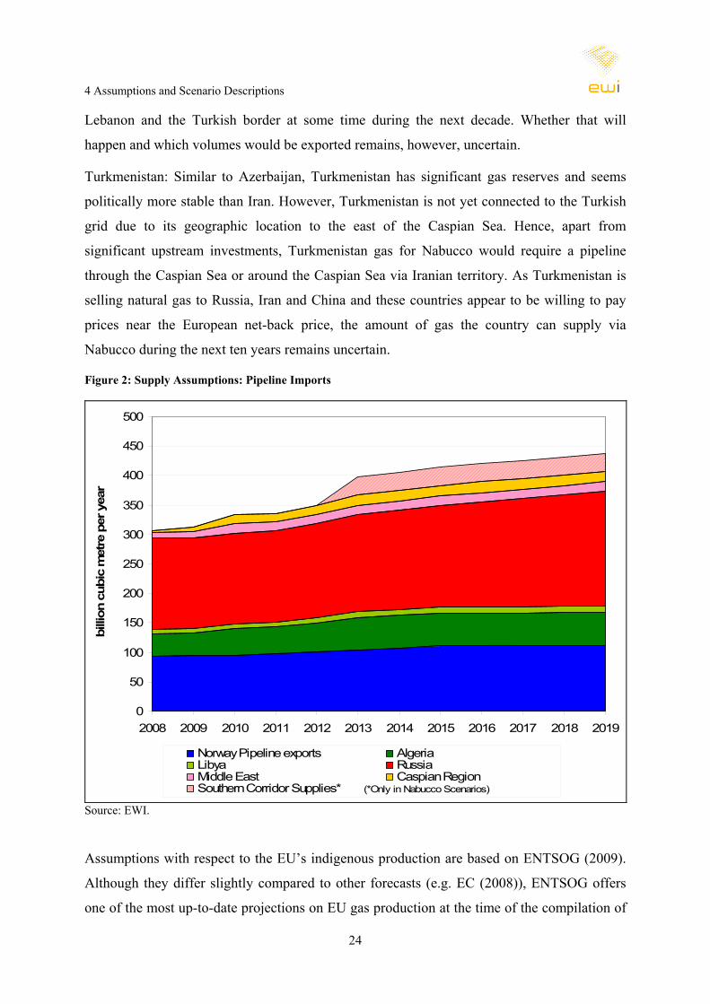
Figure 2: Supply Assumptions: Pipeline Imports
0
50
100
150
200
250
300
350
400
450
500
2008 2009 2010 2011 2012 2013 2014 2015 2016 2017 2018 2019
Norway Pipeline exports AlgeriaLibya RussiaMiddle East Caspian RegionSouthern Corridor Supplies* (*Only in Nabucco Scenarios)
billi
on c
ubic
met
re p
er y
ear
Source: EWI.
Assumptions with respect to the EU’s indigenous production are based on ENTSOG (2009).
Although they differ slightly compared to other forecasts (e.g. EC (2008)), ENTSOG offers
one of the most up-to-date projections on EU gas production at the time of the compilation of
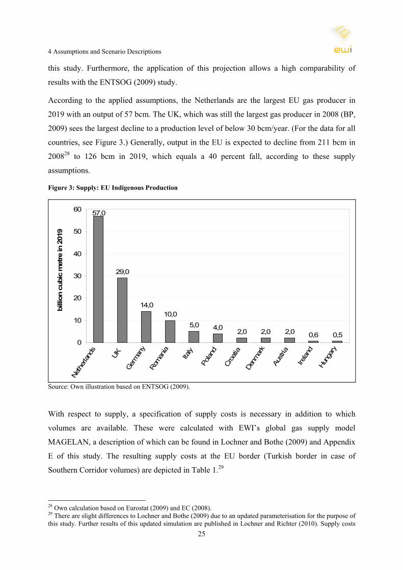
4 Assumptions and Scenario Descriptions
25
this study. Furthermore, the application of this projection allows a high comparability of
results with the ENTSOG (2009) study.
According to the applied assumptions, the Netherlands are the largest EU gas producer in
2019 with an output of 57 bcm. The UK, which was still the largest gas producer in 2008 (BP,
2009) sees the largest decline to a production level of below 30 bcm/year. (For the data for all
countries, see Figure 3.) Generally, output in the EU is expected to decline from 211 bcm in
200828 to 126 bcm in 2019, which equals a 40 percent fall, according to these supply
assumptions.
Figure 3: Supply: EU Indigenous Production
29,0
14,010,0
5,0 4,0 2,0 2,0 2,0 0,6 0,5
57,0
0
10
20
30
40
50
60
Neth
erlan
ds
UK
Germ
any
Rom
ania
Italy
Polan
d
Croa
tiaDe
nmar
k
Austr
ia
Irelan
d
Hung
ary
billi
on c
ubic
met
re in
201
9
Source: Own illustration based on ENTSOG (2009).
With respect to supply, a specification of supply costs is necessary in addition to which
volumes are available. These were calculated with EWI’s global gas supply model
MAGELAN, a description of which can be found in Lochner and Bothe (2009) and Appendix
E of this study. The resulting supply costs at the EU border (Turkish border in case of
Southern Corridor volumes) are depicted in Table 1.29
28 Own calculation based on Eurostat (2009) and EC (2008). 29 There are slight differences to Lochner and Bothe (2009) due to an updated parameterisation for the purpose of this study. Further results of this updated simulation are published in Lochner and Richter (2010). Supply costs

4 Assumptions and Scenario Descriptions
26
The interesting case thereby is the cost of LNG. As depicted in Table 1, the marginal LNG
supply in the global market is significantly higher than the marginal cost of pipeline supplies
to the European market which is quite intuitive considering that Europe is in a geographical
advantageous position in close proximity to a number of gas producing and LNG exporting
countries.
However, if Europe wants to import LNG, it has to compete with other potential LNG
importers (and all studies indicate that LNG cargos will be necessary for supplying the
European market, see also Lochner and Bothe (2009)). The price of LNG is determined by its
value in other markets as LNG suppliers, especially in an increasing global market with more
short-term trade, always have the opportunity to sell LNG in a different downstream market,
e.g. North America, Japan, South Korea, Taiwan, India, China and others. (European
importers will likewise also be prepared to redirect their LNG cargos to other destinations if
the LNG has a higher value there, which of course implies that they are able to meet their
European supply obligations through other means.)
Table 1: Supply Cost Assumptions
Supply SourceSupply Cost at
EU border[EUR / MWh]
Pipeline supplies:Norway* 6.24Russia 8.73Azerbajian** 8.26Iran** 8.06Algeria 7.13Lybia 7.51
LNG (cif to Europe):Global Marginal Supplier 19.78LNG to Europe 6.21
*Supply Cost at field; **Supply Cost at Turkish border. Source: Own calculations based on Lochner and Bothe (2009).
Hence, in long-term equilibrium pipeline gas supplies may have a cost advantage compared to
LNG imports in the European gas market (due to the high opportunity costs of LNG arising
from its value in other downstream markets).
However, situations may arise when the marginal global LNG supplier is not price setting.
Such a situation was observed in the gas market in 2009: On the LNG upstream side,
liquefaction capacities increased quickly. At the same time, global demand for LNG fell due for the EU indigenous supply were set to zero as these volumes are projected to come into the market as specified in the previous paragraph anyway.
4 Assumptions and Scenario Descriptions
27
to the economic crisis, and the extraction of unconventional gas reserves in the United States,
which led to significantly smaller LNG import demand in North America. Hence, the LNG
market became a buyer’s market where sellers were looking for the best prices globally.
Looking at prices in 2009, net-backing the United States wholesale price to Europe indicates
it was profitable to redirect LNG cargos from the US to Europe as long as European
wholesale prices exceeded 6.94 EUR/MWh (which was the case during the whole year).30
At the same time, the price for natural gas imported by pipeline via long-term contracts remai-
ned well above this threshold and the wholesale prices: e.g. the import price for Russian gas
to Germany at the German border was 17.12 EUR/MWh in August 2009 (EGM, 2009, p. 16).
Consequently, importers reduced their pipeline gas imports as much as was contractually
possible and additional LNG cargos arrived in Europe.
While this is certainly not a long-term equilibrium (global LNG supplies might decline
leading to higher LNG prices or long-term pipeline contracts may be renegotiated leading to
lower pipeline gas prices, or, more likely, both), it may, thus, happen that the global gas
demand-supply balance leads to relatively low-priced LNG coming to Europe in large
quantities. Such an oversupply situation is typically a time when new players in the gas
market can easily procure gas volumes and enter in competition with incumbent firms. Hence,
it may be relevant to investigate if such a changed price structure in the European gas market
(which certainly leads to changes in gas flows as more LNG is imported) causes additional
bottlenecks to occur in 2019 which might hamper market integration and competition in a
time of temporarily low LNG prices. Therefore, a separate scenario is conceived (see Section
4.4) with low LNG prices. Methodologically, we set the cost of LNG in this scenario equal to
those of the average LNG supplier to the European market according to Lochner and Bothe
(2009).
Another recently often debated potential source of gas is unconventional gas resources. Such
unconventional resources come in different forms with the most promising ones being coal-
bed methane (CBM; gas extracted from coal beds), shale gas (extracted from shale
30 Averages for August: Henry Hub wholesale price 3.39 US-Dollar/mmbtu = 8.14 EUR/MWh minus transport cost differential 1.20 EUR/MWh (EGM, 2009, p. 8) and assuming equal regasification tariffs in US and Europe. EIA’s natural gas database reports that LNG imports took place at these prices with significant quantities coming from the European side of the Atlantic Basin”, mainly Egypt and Norway.
4 Assumptions and Scenario Descriptions
28
formations), and tight gas (extracted from other low permeable rock formations, e.g.
sandstone). While the extraction of such resources used to be unprofitable in the past,
technological progress in recent years and economies of scale (spurred by the high gas prices
up to 2008), approximately halved production costs and made drilling in these formations in
the United States economically viable (Economist, 2010). Thanks to production from
unconventional gas resources, the United States passed Russia as the world’s largest gas
producing country in 2009. With the IEA estimating global unconventional gas resources to
total 921 trillion cubic metres (and, thus, more than five times proven conventional reserves),
there appears to be a huge potential for this production to significantly shape global gas
supply during the coming decades.
The prospects of unconventional gas production on the European continent, however, remain
to be seen. Firstly, less than five percent of the global resources are estimated to be in Europe.
Secondly, the geological and political difficulties facing unconventional production in Europe
may be much larger than in the United States. Geologically, the shale gas formations in Texas
are found between 1,500 and 2,500 metres below ground. Austrian energy company OMV, on
the other hand, estimates the promising rock formations in a basin near Vienna to be as low as
4,000 to 6,000 metres below ground making drilling significantly more expensive than in the
United States (DowJones, 2010). Politically, the new technologies applied to extract uncon-
ventional gas resources may also raise environmental concerns. Compared to conventional
gas production, the extraction involves significantly more drilling (as deposits are smaller)
and the injection of chemicals and other materials into the ground to increase permeability.
The application of such technologies may prove to be much easier in the United States than in
densely populated Europe with stricter environment protection laws (although these are also
changing in the United States to limit the pollution by unconventional gas production).
Apart from these challenges, it also has to be noted that the exploration of possible basins in
Europe, e.g. in Germany, Austria, Poland and Hungary, only began recently; shale gas
production in the United States, on the other hand, already started 15 years ago.
Hence, within the 10 year horizon of this study, European production from unconventional
gas resources is not expected to play a major role.31
31 Data and facts on unconventional resources reported in this section are largely based on articles in Economist (2010) and DowJones (2010).
4 Assumptions and Scenario Descriptions
29
However, this does not mean that unconventional gas production does not have an impact on
the European gas market, even today. The significant unconventional gas production in the
United States means the country’s import demand is much lower than was expected just a few
years ago. Many of the LNG upstream facilities entering operation around the world between
2009 and 2012 were meant to cater this demand when they were planned. With lower demand
for LNG in North America, these volumes are, thus, to a larger extend available to other mar-
kets including Europe. In combination with the economic crisis in 2008 to 2010, this already
caused the LNG glut with record numbers of LNG cargos coming to Europe in 2009 and
2010.
In the future, a global natural gas resource base broadened by unconventional resources may
also benefit gas consumers in Europe as it enables larger supply diversification. This limits
the dependency on individual gas sources or supply countries and the market power of
countries with conventional gas reserves, which in turn enhances upstream competition and
security of supply.
With respect to the supply assumptions presented in this section, it has to be noted that these
have a significant impact on the results. Apart from supply volumes, the largest impact arises
from relative supply costs, in particular of LNG relative to pipeline gas. This uncertainty is
taken into account through scenario analysis as relative LNG prices are varied between sce-
narios, see Section 4.4.
4.2 Demand Assumptions
With respect to demand, two scenarios are applied in this study. Again, as the projection of
the development of gas consumption itself is not at the focus of this study, these demand
scenarios are based on publicly available studies by other institutions. With the aim of
covering a wide range of possible demand developments and selecting projections based on
data provided by both the gas industry and policy institutions, the following two demand
scenarios are compiled:
• EWI/ERGEG demand scenario based on EC (2008) and EC (2009),
• ENTSOG demand scenario based on ENTSOG (2009).
4 Assumptions and Scenario Descriptions
30
Compared to other available studies, they have the advantage of being relatively up-to-date at
the time of the compilation of this study and offering a relatively high granularity of data with
respect to countries (and sectors in case of EC (2008)).
EWI/ERGEG demand scenario:
This scenario is based on the Baseline scenario published by the European Commission in its
report “European Energy and Transport – Trends to 2030, 2007 Update” (EC, 2008). The ori-
ginal scenario assumes a gas demand growth rate of 0.9 percent annually between 2010 and
2020 of which the power sector growth amounts to 1.5 and the all other sectors together fea-
ture a growth rate of 0.6 percent per year. As an official EU Commission projection based on
consistent assumptions regarding economic development, it is selected as the Reference – and
therefore most-likely – demand scenario for this study. The detailed provision of data by
country and sector (power- vs. non-power sector) and all EU member states by EC (2008)
allow an application of country-specific seasonal demand profiles incorporated in the TIGER
model (see Chapter 3).
However, one of the major disadvantages of the original EC (2008) Baseline scenario is that it
is not up-to-date as it is based on 2007 data compiled in 2008. Therefore, the data is adjusted
to the demand declines following the 2009 economic crisis as follows: A regression of non-
power and power sector gas demand is performed (using the GDP and gas demand data from
EC (2008) for the 2000 to 2010 time period) to establish the relationship between GDP and
sectoral gas consumption on a country-level. Using current GDP data for 2009 and 2010
(forecast)32 the estimators are then used to correct the original EC (2008) non-power and
power sector demand projections for the two years and for each country respectively. After
2009, the demand data is projected to increase with the original EC (2008) growth rates. 33
The resulting average annual demand growth between 2009 and 2019 is 0.8 percent.
The Baseline Scenario in its original form (EC, 2008) and the adapted EWI/ERGEG version
are displayed in Figure 4. (All numerical assumptions by country can also be found in Table
10 in the Appendix (page 121)).
32 GDP forecasts published by Eurostat data have been used. 33 For more details on the underlying assumptions for future GDP growth during and after the financial crisis see EC (2009).

4 Assumptions and Scenario Descriptions
31
ENTSOG demand scenario:
Demand projections are associated with some degree of uncertainty. Therefore, we include a
second demand scenario which equals the ENTSOG (2009) annual demand assumptions. This
scenario is a suitable complement to the first demand scenario: Firstly, the EWI/ERGEG
demand (especially after adjusting for the economic crisis) constitutes a rather conservative
projection for the development of gas consumption (also in context of other studies, e.g. IEA
(2008), EIA (2009)); the ENTSOG one presumes higher demand growth of 1.4 percent
annually. Secondly, maintaining a high degree of comparability of this study with ENTSOG
(2009) is in the interest of ERGEG and relevant stakeholders. This is ensured by applying a
second demand scenario along the lines of ENTSOG (2009). Together with the EWI/ERGEG
demand assumption, the ENTSOG scenario is depicted in Figure 4. The demand difference
between the ENTSOG and EWI/ERGEG Scenario is about 49 bcm in 2019. Hence, the two
scenarios cover a sufficient bandwidth of possible gas demand developments until 2019.
Figure 4: Demand Scenarios
400
420
440
460
480
500
520
540
560
580
600
2008 2009 2010 2011 2012 2013 2014 2015 2016 2017 2018 2019
EC (2008) dataEWI/ERGEG Demand (adapted EC(2008) data)ENTSOG (2009)
billi
on c
ubic
met
re p
er y
ear
Source: Own calculation based on ENTSOG (2009), EC (2008) / IEA (2009) and EWI assumptions.
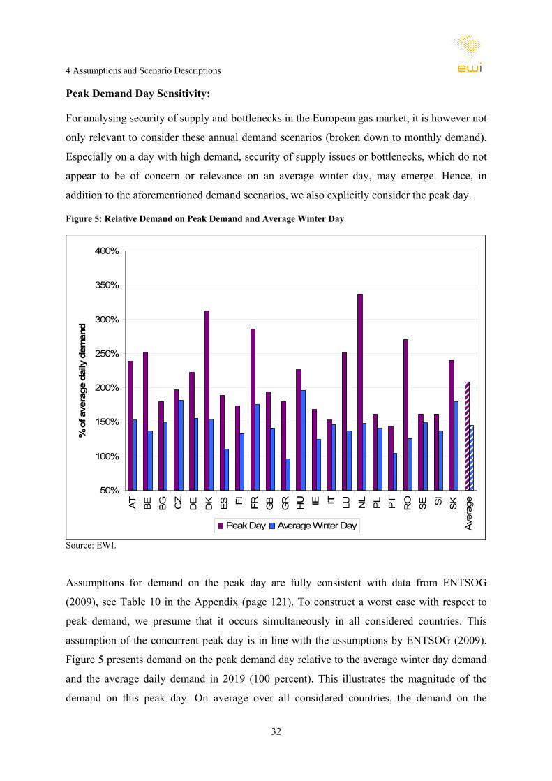
4 Assumptions and Scenario Descriptions
32
Peak Demand Day Sensitivity:
For analysing security of supply and bottlenecks in the European gas market, it is however not
only relevant to consider these annual demand scenarios (broken down to monthly demand).
Especially on a day with high demand, security of supply issues or bottlenecks, which do not
appear to be of concern or relevance on an average winter day, may emerge. Hence, in
addition to the aforementioned demand scenarios, we also explicitly consider the peak day.
Figure 5: Relative Demand on Peak Demand and Average Winter Day
50%
100%
150%
200%
250%
300%
350%
400%
AT
BE
BG CZ
DE
DK
ES FI FR GB
GR
HU IE IT LU NL
PL
PT
RO
SE SI
SK
Ave
rage
% o
f ave
rage
dai
ly d
eman
d
Peak Day Average Winter Day
Source: EWI.
Assumptions for demand on the peak day are fully consistent with data from ENTSOG
(2009), see Table 10 in the Appendix (page 121). To construct a worst case with respect to
peak demand, we presume that it occurs simultaneously in all considered countries. This
assumption of the concurrent peak day is in line with the assumptions by ENTSOG (2009).
Figure 5 presents demand on the peak demand day relative to the average winter day demand
and the average daily demand in 2019 (100 percent). This illustrates the magnitude of the
demand on this peak day. On average over all considered countries, the demand on the
4 Assumptions and Scenario Descriptions
33
average winter day is about 48 percent higher than the average daily demand throughout the
year. On the peak day, demand is another 40 percent higher (or plus 106 percent above the
average demand day).34
(All numerical demand data for 2019 can be obtained from Table 10 in the Appendix.)
There are, however, significant differences between countries which might have implications
on the results regarding the peak day simulations: According to these assumptions, the peak
day has the relatively highest demand in the Netherlands, Denmark and France. In Poland and
Italy, on the other hand, demand on the peak day barely exceeds demand on an average winter
day.
4.3 Infrastructure Assumptions
The assumptions concerning the major infrastructure components of the model simulations
are presented in this section.
This includes which new projects are commissioned and which existing once are expanded
relative to the status quo (December 2009).
As the focus of the subsequent investigations is the year 2019, it has to be noted that the
assumed commissioning date within the 2010 to 2018 period is not relevant for the model
results. However, it is of course important if the project is commissioned by 2019 or not. For
selected pipeline projects, this is varied between scenarios, i.e. some scenarios assume that a
pipeline project is postponed to after 2019 or cancelled (see next section). In this section, all
infrastructure projects included in at least one of the scenarios are presented with respect to
assumptions concerning capacities, routes and start-up dates (for pipelines, LNG
regasification terminals and storages).
Import Pipeline Projects
The major import pipeline projects (and their assumed routes) included in this study are
depicted in Figure 6. These are:
34 We assume the peak demand day to be in winter on the fourth Wednesday in January.
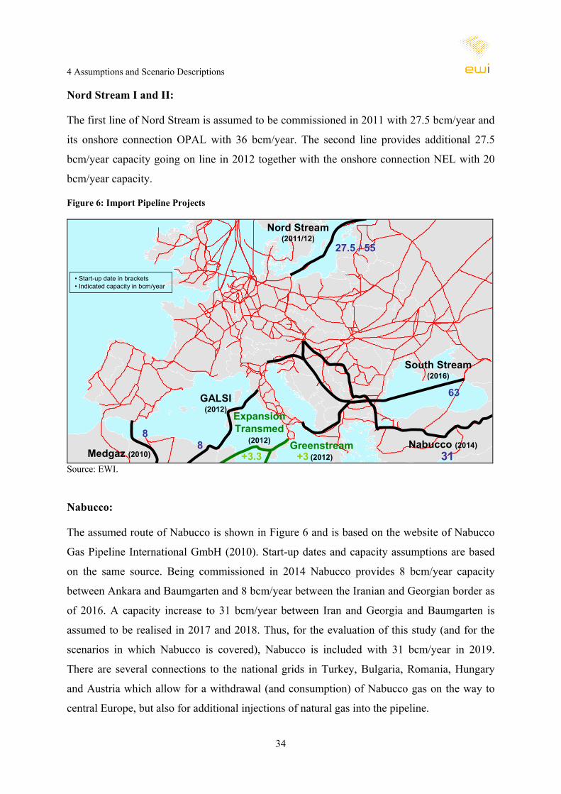
4 Assumptions and Scenario Descriptions
34
Nord Stream I and II:
The first line of Nord Stream is assumed to be commissioned in 2011 with 27.5 bcm/year and
its onshore connection OPAL with 36 bcm/year. The second line provides additional 27.5
bcm/year capacity going on line in 2012 together with the onshore connection NEL with 20
bcm/year capacity.
Figure 6: Import Pipeline Projects
Nord Stream(2011/12)
South Stream(2016)
Nabucco (2014)Medgaz (2010)
GALSI(2012)
Expansion Transmed
(2012) Greenstream(2012)
27.5 / 55
63
318
8
+3.3 +3
• Start-up date in brackets• Indicated capacity in bcm/year
Source: EWI.
Nabucco:
The assumed route of Nabucco is shown in Figure 6 and is based on the website of Nabucco
Gas Pipeline International GmbH (2010). Start-up dates and capacity assumptions are based
on the same source. Being commissioned in 2014 Nabucco provides 8 bcm/year capacity
between Ankara and Baumgarten and 8 bcm/year between the Iranian and Georgian border as
of 2016. A capacity increase to 31 bcm/year between Iran and Georgia and Baumgarten is
assumed to be realised in 2017 and 2018. Thus, for the evaluation of this study (and for the
scenarios in which Nabucco is covered), Nabucco is included with 31 bcm/year in 2019.
There are several connections to the national grids in Turkey, Bulgaria, Romania, Hungary
and Austria which allow for a withdrawal (and consumption) of Nabucco gas on the way to
central Europe, but also for additional injections of natural gas into the pipeline.
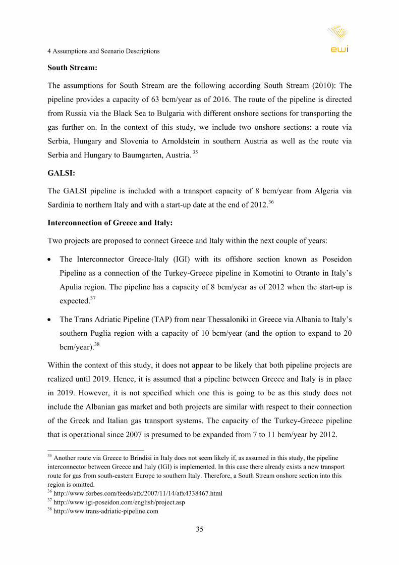
4 Assumptions and Scenario Descriptions
35
South Stream:
The assumptions for South Stream are the following according South Stream (2010): The
pipeline provides a capacity of 63 bcm/year as of 2016. The route of the pipeline is directed
from Russia via the Black Sea to Bulgaria with different onshore sections for transporting the
gas further on. In the context of this study, we include two onshore sections: a route via
Serbia, Hungary and Slovenia to Arnoldstein in southern Austria as well as the route via
Serbia and Hungary to Baumgarten, Austria. 35
GALSI:
The GALSI pipeline is included with a transport capacity of 8 bcm/year from Algeria via
Sardinia to northern Italy and with a start-up date at the end of 2012.36
Interconnection of Greece and Italy:
Two projects are proposed to connect Greece and Italy within the next couple of years:
• The Interconnector Greece-Italy (IGI) with its offshore section known as Poseidon
Pipeline as a connection of the Turkey-Greece pipeline in Komotini to Otranto in Italy’s
Apulia region. The pipeline has a capacity of 8 bcm/year as of 2012 when the start-up is
expected.37
• The Trans Adriatic Pipeline (TAP) from near Thessaloniki in Greece via Albania to Italy’s
southern Puglia region with a capacity of 10 bcm/year (and the option to expand to 20
bcm/year).38
Within the context of this study, it does not appear to be likely that both pipeline projects are
realized until 2019. Hence, it is assumed that a pipeline between Greece and Italy is in place
in 2019. However, it is not specified which one this is going to be as this study does not
include the Albanian gas market and both projects are similar with respect to their connection
of the Greek and Italian gas transport systems. The capacity of the Turkey-Greece pipeline
that is operational since 2007 is presumed to be expanded from 7 to 11 bcm/year by 2012.
35 Another route via Greece to Brindisi in Italy does not seem likely if, as assumed in this study, the pipeline interconnector between Greece and Italy (IGI) is implemented. In this case there already exists a new transport route for gas from south-eastern Europe to southern Italy. Therefore, a South Stream onshore section into this region is omitted. 36 http://www.forbes.com/feeds/afx/2007/11/14/afx4338467.html 37 http://www.igi-poseidon.com/english/project.asp 38 http://www.trans-adriatic-pipeline.com
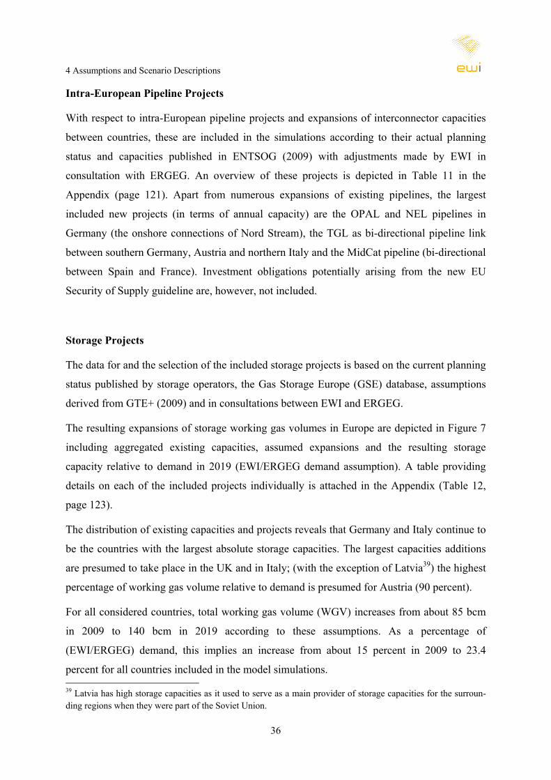
4 Assumptions and Scenario Descriptions
36
Intra-European Pipeline Projects
With respect to intra-European pipeline projects and expansions of interconnector capacities
between countries, these are included in the simulations according to their actual planning
status and capacities published in ENTSOG (2009) with adjustments made by EWI in
consultation with ERGEG. An overview of these projects is depicted in Table 11 in the
Appendix (page 121). Apart from numerous expansions of existing pipelines, the largest
included new projects (in terms of annual capacity) are the OPAL and NEL pipelines in
Germany (the onshore connections of Nord Stream), the TGL as bi-directional pipeline link
between southern Germany, Austria and northern Italy and the MidCat pipeline (bi-directional
between Spain and France). Investment obligations potentially arising from the new EU
Security of Supply guideline are, however, not included.
Storage Projects
The data for and the selection of the included storage projects is based on the current planning
status published by storage operators, the Gas Storage Europe (GSE) database, assumptions
derived from GTE+ (2009) and in consultations between EWI and ERGEG.
The resulting expansions of storage working gas volumes in Europe are depicted in Figure 7
including aggregated existing capacities, assumed expansions and the resulting storage
capacity relative to demand in 2019 (EWI/ERGEG demand assumption). A table providing
details on each of the included projects individually is attached in the Appendix (Table 12,
page 123).
The distribution of existing capacities and projects reveals that Germany and Italy continue to
be the countries with the largest absolute storage capacities. The largest capacities additions
are presumed to take place in the UK and in Italy; (with the exception of Latvia39) the highest
percentage of working gas volume relative to demand is presumed for Austria (90 percent).
For all considered countries, total working gas volume (WGV) increases from about 85 bcm
in 2009 to 140 bcm in 2019 according to these assumptions. As a percentage of
(EWI/ERGEG) demand, this implies an increase from about 15 percent in 2009 to 23.4
percent for all countries included in the model simulations. 39 Latvia has high storage capacities as it used to serve as a main provider of storage capacities for the surroun-ding regions when they were part of the Soviet Union.

4 Assumptions and Scenario Descriptions
37
Figure 7: Storage Working Gas Volumes in Europe
0
5
10
15
20
25
30A
ustri
a
Bel
gium
Bul
garia
Cro
atia
Cze
ch R
epub
lic
Den
mar
k
Fran
ce
Ger
man
y
Hun
gary
Irlan
d
Italy
Latv
ia
Net
herla
nds
Pol
and
Por
tuga
l
Rom
ania
Ser
bia
Slo
vak
Rep
ublic
Spa
in
Sw
eden
Turk
ey UK
Wor
king
Gas
Vol
ume
(WG
V) in
bcm
0%
10%
20%
30%
40%
50%
60%
70%
80%
90%
100%
Per
cent
age
of E
WI/E
RG
EG d
eman
d
Existing (as of 12/2009) Assumed additions until 2019 WGV as percentage of demand in 2019
Source: EWI.
LNG Import (Regasification) Terminal Projects
The data assumptions for the regasification terminals included in the simulation are based on
official publications of the terminal operators and databases as for example provided by GLE.
Similar to storage, they have been adapted in coordination with ERGEG to obtain a realistic
picture of LNG import capacity expansions in Europe until 2019. A list of all terminals and
expansion stages is displayed in Table 13 on page 125. (The table is also accompanied by a
map showing the location of terminals (Figure 57).) Figure 8 illustrates existing capacities and
presumed capacity additions by country. Thereby, Spain remains the country with the largest
nominal import capacities. Large increases are also expected for the Netherlands and France
(but less so for the UK after 2010 as the country’s capacity has already significantly increased
in 2009). Total annual LNG import capacity in Europe (including Turkey) increases by almost
70 percent from 165 bcm in 2009/2010 to 279 bcm in 2009.
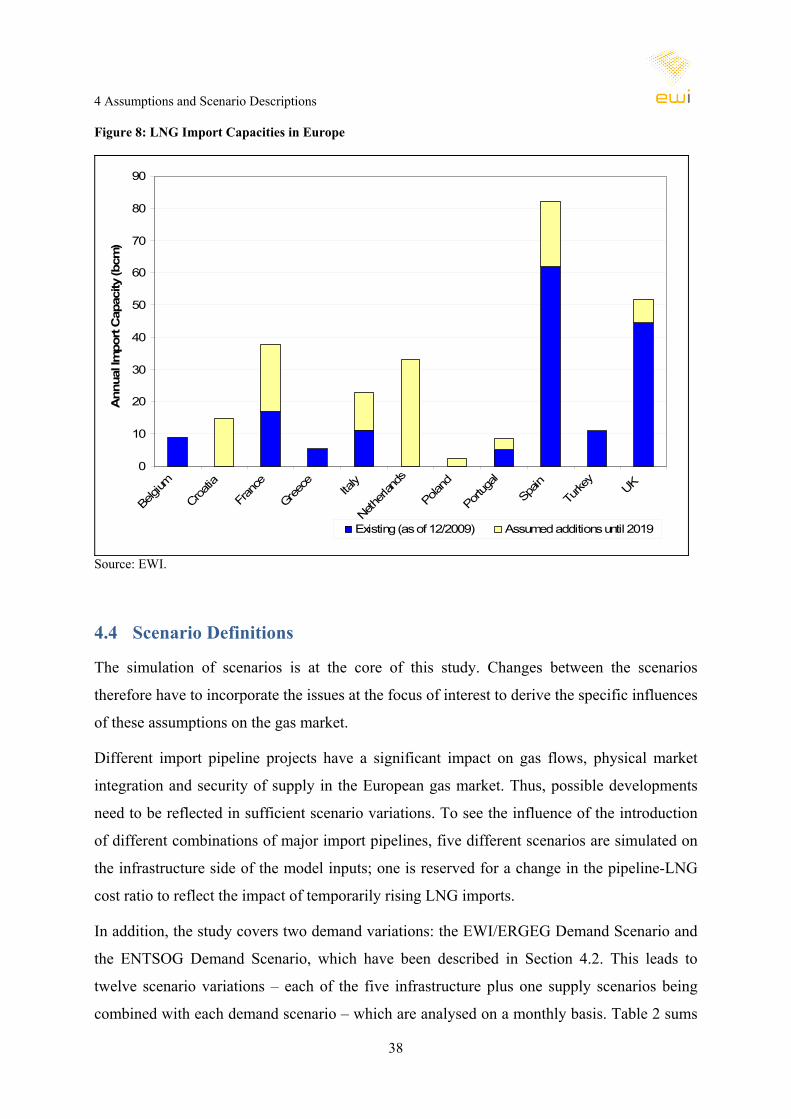
4 Assumptions and Scenario Descriptions
38
Figure 8: LNG Import Capacities in Europe
0
10
20
30
40
50
60
70
80
90
Belgi
um
Croatia
Fran
ce
Greece Ita
ly
Netherl
ands
Polan
d
Portu
gal
Spain
Turke
yUK
Ann
ual I
mpo
rt C
apac
ity (b
cm)
Existing (as of 12/2009) Assumed additions until 2019
Source: EWI.
4.4 Scenario Definitions
The simulation of scenarios is at the core of this study. Changes between the scenarios
therefore have to incorporate the issues at the focus of interest to derive the specific influences
of these assumptions on the gas market.
Different import pipeline projects have a significant impact on gas flows, physical market
integration and security of supply in the European gas market. Thus, possible developments
need to be reflected in sufficient scenario variations. To see the influence of the introduction
of different combinations of major import pipelines, five different scenarios are simulated on
the infrastructure side of the model inputs; one is reserved for a change in the pipeline-LNG
cost ratio to reflect the impact of temporarily rising LNG imports.
In addition, the study covers two demand variations: the EWI/ERGEG Demand Scenario and
the ENTSOG Demand Scenario, which have been described in Section 4.2. This leads to
twelve scenario variations – each of the five infrastructure plus one supply scenarios being
combined with each demand scenario – which are analysed on a monthly basis. Table 2 sums
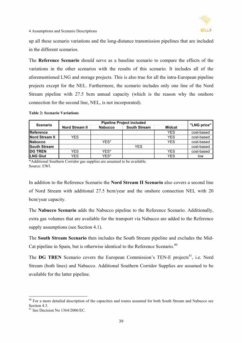
4 Assumptions and Scenario Descriptions
39
up all these scenario variations and the long-distance transmission pipelines that are included
in the different scenarios.
The Reference Scenario should serve as a baseline scenario to compare the effects of the
variations in the other scenarios with the results of this scenario. It includes all of the
aforementioned LNG and storage projects. This is also true for all the intra-European pipeline
projects except for the NEL. Furthermore, the scenario includes only one line of the Nord
Stream pipeline with 27.5 bcm annual capacity (which is the reason why the onshore
connection for the second line, NEL, is not incorporated).
Table 2: Scenario Variations
Nord Stream II Nabucco South Stream MidcatReference YES cost-basedNord Stream II YES YES cost-basedNabucco YES* YES cost-basedSouth Stream YES cost-basedDG TREN YES YES* YES cost-basedLNG Glut YES YES* YES low
Scenario Pipeline Project included "LNG price"
*Additional Southern Corridor gas supplies are assumed to be available. Source: EWI.
In addition to the Reference Scenario the Nord Stream II Scenario also covers a second line
of Nord Stream with additional 27.5 bcm/year and the onshore connection NEL with 20
bcm/year capacity.
The Nabucco Scenario adds the Nabucco pipeline to the Reference Scenario. Additionally,
extra gas volumes that are available for the transport via Nabucco are added to the Reference
supply assumptions (see Section 4.1).
The South Stream Scenario then includes the South Stream pipeline and excludes the Mid-
Cat pipeline in Spain, but is otherwise identical to the Reference Scenario.40
The DG TREN Scenario covers the European Commission’s TEN-E projects41, i.e. Nord
Stream (both lines) and Nabucco. Additional Southern Corridor Supplies are assumed to be
available for the latter pipeline.
40 For a more detailed description of the capacities and routes assumed for both South Stream and Nabucco see Section 4.3. 41 See Decision No 1364/2006/EC.

4 Assumptions and Scenario Descriptions
40
The influence of an exclusion of the inner European MidCat pipeline between north-eastern
Spain and southern France is also analysed in addition to the major import pipelines.
Therefore it has only been excluded in the South Stream Scenario as South Stream should not
have any significant effect on the Spanish gas market.
In the scenario LNG Glut, the relative LNG costs are assumed to be lower (see Section 4.1).
Otherwise, it is identical to the DG TREN Scenario. The motivation for this relative cost
variation is to specifically see the effects on market integration congestion in the infra-
structure system caused by temporarily low LNG prices. Although relatively lower LNG costs
(compared to pipeline gas) may not be a long-term equilibrium for the European market, such
an LNG oversupply situation could arise temporarily in the global gas market (as it did in
2009). To ensure competition, physical market integration plays an important role – especially
in times of oversupply which usually is a chance for new market entrants to procure gas at
low prices. In such a situation, bottlenecks in the system could hamper market entry and block
consumers from accessing cheaper gas supplies (imported as LNG).
Furthermore, six sensitivities (one per infrastructure scenario) covering a peak day analysis
(based on the higher ENTSOG demand) are implemented. Moreover, five security of supply
sensitivities simulating a disruption of the Russian pipeline gas supplies through Ukraine, and
another five sensitivities simulating a disruption of Algerian exports are analysed. (The LNG
Glut scenario is not considered in the SoS simulations as in such a stress situation,
infrastructure is the most relevant assumption. In this respect, the LNG Glut Scenario is
identical to the DG TREN scenario.) The duration of the stress situations is presumed to last
one month; however, both are modelled in simulations of the whole year 2019 with a daily
granularity.
The twelve scenarios cover a wide range of potential demand, upstream (relative LNG) price
and infrastructure developments (with respect to the major projects). They allow an
encompassing investigation of these major projects, physical market integration and security
of supply stress scenarios. The interpretation of results thereby focuses on the year 2019.
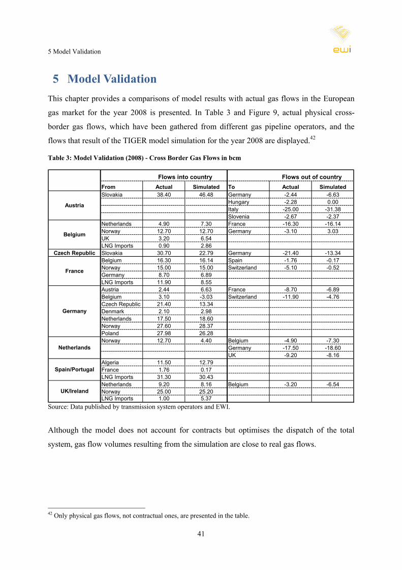
5 Model Validation
41
5 Model Validation This chapter provides a comparisons of model results with actual gas flows in the European
gas market for the year 2008 is presented. In Table 3 and Figure 9, actual physical cross-
border gas flows, which have been gathered from different gas pipeline operators, and the
flows that result of the TIGER model simulation for the year 2008 are displayed.42
Table 3: Model Validation (2008) - Cross Border Gas Flows in bcm
From Actual Simulated To Actual SimulatedSlovakia 38.40 46.48 Germany -2.44 -6.63
Hungary -2.28 0.00Italy -25.00 -31.38Slovenia -2.67 -2.37
Netherlands 4.90 7.30 France -16.30 -16.14Norway 12.70 12.70 Germany -3.10 3.03UK 3.20 6.54LNG Imports 0.90 2.86
Czech Republic Slovakia 30.70 22.79 Germany -21.40 -13.34Belgium 16.30 16.14 Spain -1.76 -0.17Norway 15.00 15.00 Switzerland -5.10 -0.52Germany 8.70 6.89LNG Imports 11.90 8.55Austria 2.44 6.63 France -8.70 -6.89Belgium 3.10 -3.03 Switzerland -11.90 -4.76Czech Republic 21.40 13.34Denmark 2.10 2.98Netherlands 17.50 18.60Norway 27.60 28.37Poland 27.98 26.28Norway 12.70 4.40 Belgium -4.90 -7.30
Germany -17.50 -18.60UK -9.20 -8.16
Algeria 11.50 12.79France 1.76 0.17LNG Imports 31.30 30.43Netherlands 9.20 8.16 Belgium -3.20 -6.54Norway 25.00 25.20LNG Imports 1.00 5.37
Flows into country Flows out of country
Netherlands
UK/Ireland
Spain/Portugal
Austria
Germany
Belgium
France
Source: Data published by transmission system operators and EWI.
Although the model does not account for contracts but optimises the dispatch of the total
system, gas flow volumes resulting from the simulation are close to real gas flows.
42 Only physical gas flows, not contractual ones, are presented in the table.
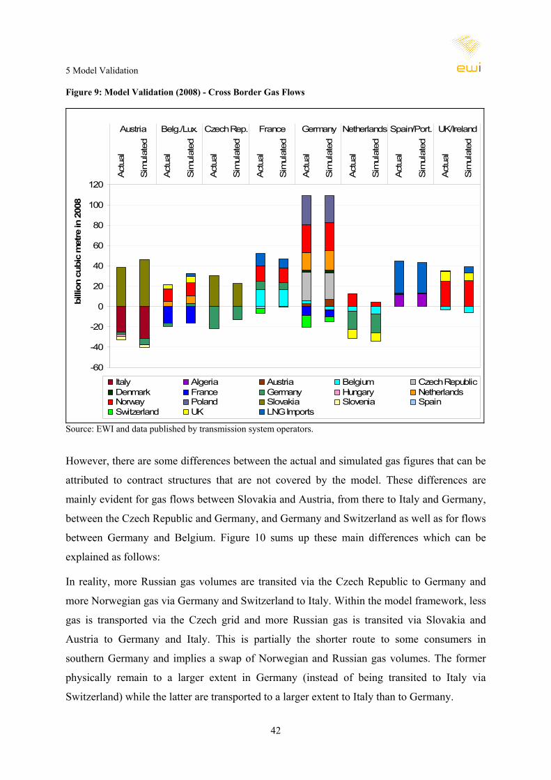
5 Model Validation
42
Figure 9: Model Validation (2008) - Cross Border Gas Flows
-60
-40
-20
0
20
40
60
80
100
120
Act
ual
Sim
ulat
ed
Act
ual
Sim
ulat
ed
Act
ual
Sim
ulat
ed
Act
ual
Sim
ulat
ed
Act
ual
Sim
ulat
ed
Act
ual
Sim
ulat
ed
Act
ual
Sim
ulat
ed
Act
ual
Sim
ulat
ed
Austria Belg./Lux. Czech Rep. France Germany Netherlands Spain/Port. UK/Ireland
billi
on c
ubic
met
re in
200
8
Italy Algeria Austria Belgium Czech RepublicDenmark France Germany Hungary NetherlandsNorway Poland Slovakia Slovenia SpainSwitzerland UK LNG Imports
Source: EWI and data published by transmission system operators.
However, there are some differences between the actual and simulated gas figures that can be
attributed to contract structures that are not covered by the model. These differences are
mainly evident for gas flows between Slovakia and Austria, from there to Italy and Germany,
between the Czech Republic and Germany, and Germany and Switzerland as well as for flows
between Germany and Belgium. Figure 10 sums up these main differences which can be
explained as follows:
In reality, more Russian gas volumes are transited via the Czech Republic to Germany and
more Norwegian gas via Germany and Switzerland to Italy. Within the model framework, less
gas is transported via the Czech grid and more Russian gas is transited via Slovakia and
Austria to Germany and Italy. This is partially the shorter route to some consumers in
southern Germany and implies a swap of Norwegian and Russian gas volumes. The former
physically remain to a larger extent in Germany (instead of being transited to Italy via
Switzerland) while the latter are transported to a larger extent to Italy than to Germany.
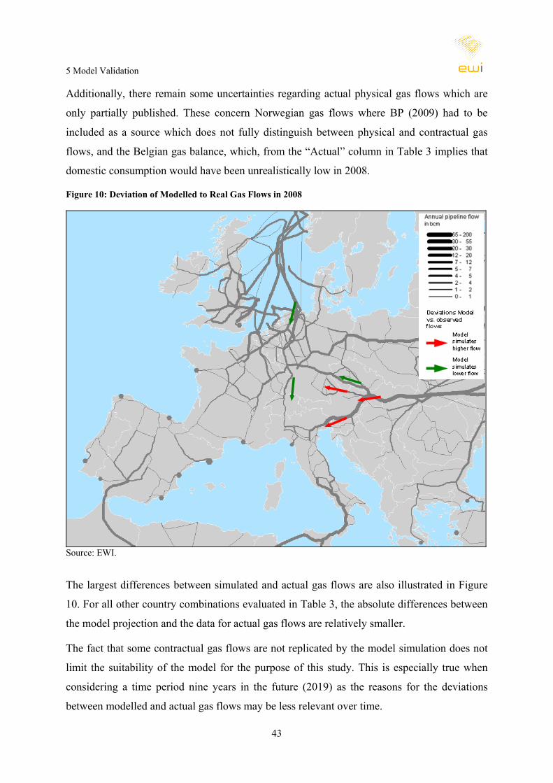
5 Model Validation
43
Additionally, there remain some uncertainties regarding actual physical gas flows which are
only partially published. These concern Norwegian gas flows where BP (2009) had to be
included as a source which does not fully distinguish between physical and contractual gas
flows, and the Belgian gas balance, which, from the “Actual” column in Table 3 implies that
domestic consumption would have been unrealistically low in 2008.
Figure 10: Deviation of Modelled to Real Gas Flows in 2008
Source: EWI.
The largest differences between simulated and actual gas flows are also illustrated in Figure
10. For all other country combinations evaluated in Table 3, the absolute differences between
the model projection and the data for actual gas flows are relatively smaller.
The fact that some contractual gas flows are not replicated by the model simulation does not
limit the suitability of the model for the purpose of this study. This is especially true when
considering a time period nine years in the future (2019) as the reasons for the deviations
between modelled and actual gas flows may be less relevant over time.
5 Model Validation
44
Firstly, with increasing separation (unbundling) of gas transport and trading and the efforts by
national regulators to enhance efficiency and improve network access, one can expect
European gas transportation to become more efficient. Hence, more of the efficient swaps
presumed by the model might actually be implemented in reality.
The second reason which causes the modelled flows to deviate from actual gas flows might be
differences in gas qualities for natural gas from different sources: The applied TIGER Model
only distinguishes between high (H) and low (L) calorific gas, but not between H gas from
different sources (Norway vs. Russia in this case) which might hamper the implementation of
gas swaps in the short-term. However, with the medium term view of this study, this is less of
a constraint as consumers can adapt to changes in gas qualities. As indigenous European
production declines, imports increase and new supply sources (LNG, Caspian region) are
projected to be tapped for the European market, this may have to happen anyway.
Hence, the medium-term perspective applied in this study and the increasing efficiency in the
European gas market may even further increase the overlap of model simulations and actual
gas flows.
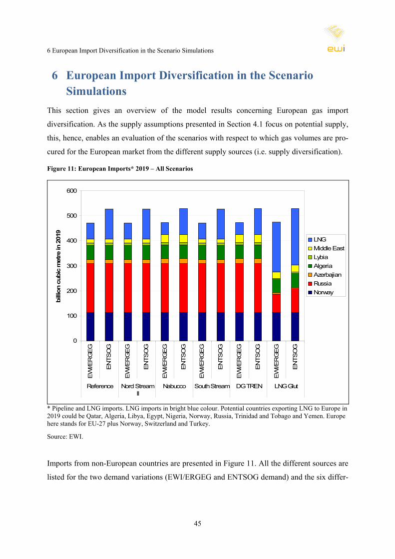
6 European Import Diversification in the Scenario Simulations
45
6 European Import Diversification in the Scenario Simulations
This section gives an overview of the model results concerning European gas import
diversification. As the supply assumptions presented in Section 4.1 focus on potential supply,
this, hence, enables an evaluation of the scenarios with respect to which gas volumes are pro-
cured for the European market from the different supply sources (i.e. supply diversification).
Figure 11: European Imports* 2019 – All Scenarios
0
100
200
300
400
500
600
EW
I/ER
GE
G
EN
TSO
G
EW
I/ER
GE
G
EN
TSO
G
EW
I/ER
GE
G
EN
TSO
G
EW
I/ER
GE
G
EN
TSO
G
EW
I/ER
GE
G
EN
TSO
G
EW
I/ER
GE
G
EN
TSO
G
Reference Nord StreamII
Nabucco South Stream DG TREN LNG Glut
billi
on c
ubic
met
re in
201
9
LNGMiddle EastLybiaAlgeriaAzerbajianRussiaNorway
* Pipeline and LNG imports. LNG imports in bright blue colour. Potential countries exporting LNG to Europe in 2019 could be Qatar, Algeria, Libya, Egypt, Nigeria, Norway, Russia, Trinidad and Tobago and Yemen. Europe here stands for EU-27 plus Norway, Switzerland and Turkey.
Source: EWI.
Imports from non-European countries are presented in Figure 11. All the different sources are
listed for the two demand variations (EWI/ERGEG and ENTSOG demand) and the six differ-
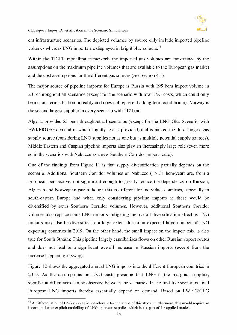
6 European Import Diversification in the Scenario Simulations
46
ent infrastructure scenarios. The depicted volumes by source only include imported pipeline
volumes whereas LNG imports are displayed in bright blue colours.43
Within the TIGER modelling framework, the imported gas volumes are constrained by the
assumptions on the maximum pipeline volumes that are available to the European gas market
and the cost assumptions for the different gas sources (see Section 4.1).
The major source of pipeline imports for Europe is Russia with 195 bcm import volume in
2019 throughout all scenarios (except for the scenario with low LNG costs, which could only
be a short-term situation in reality and does not represent a long-term equilibrium). Norway is
the second largest supplier in every scenario with 112 bcm.
Algeria provides 55 bcm throughout all scenarios (except for the LNG Glut Scenario with
EWI/ERGEG demand in which slightly less is provided) and is ranked the third biggest gas
supply source (considering LNG supplies not as one but as multiple potential supply sources).
Middle Eastern and Caspian pipeline imports also play an increasingly large role (even more
so in the scenarios with Nabucco as a new Southern Corridor import route).
One of the findings from Figure 11 is that supply diversification partially depends on the
scenario. Additional Southern Corridor volumes on Nabucco (+/- 31 bcm/year) are, from a
European perspective, not significant enough to greatly reduce the dependency on Russian,
Algerian and Norwegian gas; although this is different for individual countries, especially in
south-eastern Europe and when only considering pipeline imports as these would be
diversified by extra Southern Corridor volumes. However, additional Southern Corridor
volumes also replace some LNG imports mitigating the overall diversification effect as LNG
imports may also be diversified to a large extent due to an expected large number of LNG
exporting countries in 2019. On the other hand, the small impact on the import mix is also
true for South Stream: This pipeline largely cannibalises flows on other Russian export routes
and does not lead to a significant overall increase in Russian imports (except from the
increase happening anyway).
Figure 12 shows the aggregated annual LNG imports into the different European countries in
2019. As the assumptions on LNG costs presume that LNG is the marginal supplier,
significant differences can be observed between the scenarios. In the first five scenarios, total
European LNG imports thereby essentially depend on demand. Based on EWI/ERGEG 43 A differentiation of LNG sources is not relevant for the scope of this study. Furthermore, this would require an incorporation or explicit modelling of LNG upstream supplies which is not part of the applied model.
6 European Import Diversification in the Scenario Simulations
47
demand assumptions, LNG imports amount between 48 and 64 bcm (about 48 bcm in the
scenarios with Nabucco (Nabucco and DG TREN) and about 64 bcm without Nabucco).
Figure 12: LNG Imports per Country in 2019
0
50
100
150
200
250
EW
I/ER
GE
G
EN
TSO
G
EW
I/ER
GE
G
EN
TSO
G
EW
I/ER
GE
G
EN
TSO
G
EW
I/ER
GE
G
EN
TSO
G
EW
I/ER
GE
G
EN
TSO
G
EW
I/ER
GE
G
EN
TSO
G
Reference Nord StreamII
Nabucco South Stream DG TREN LNG Glut
billi
on c
ubic
met
re in
201
9
PolandGreecePortugalCroatiaBelgium TurkeyItalyNetherlandsFranceSpainUK
Source: EWI.
With the higher ENTSOG demand, more LNG is imported: between 103 and 120 bcm
depending on the scenario (with about 103 bcm in the scenarios with Nabucco and about 120
bcm without Nabucco).
Thus, it can be concluded that less LNG is needed with Nabucco bringing extra gas volumes
to the European market. Hence, LNG acts as an implicit swing supplier in this medium term
view: If more pipeline gas is contracted to come to Europe, less LNG is imported and vice
versa.
In case of low LNG costs (Scenario LNG GLUT), pipeline gas is crowded out starting with
the most expensive sources which is gas from Libya and Azerbaijan based on the modelling
assumptions. However, Russian imports are also reduced by 62 percent to 74 bcm in the LNG
Glut Scenario with EWI/ERGEG demand and by 51 percent to 95 bcm for the ENTSOG
6 European Import Diversification in the Scenario Simulations
48
demand case (see Figure 12). With the assumed LNG capacities, it is hence theoretically
possible to import more than 200 bcm of LNG annually in 2019 if LNG prices are low and
contractual obligations (from Take-Or-Pay clauses) to import pipeline gas can be partly
reduced. For all considered LNG terminals (see Section 4.3), this implies an average
utilisation of 70 percent in the EWI/ERGEG demand scenario and of 80 percent with
ENTSOG demand.
Spain, the UK and France are the countries with the highest LNG imports in 2019 throughout
all scenarios. The Spanish LNG import volumes differ between 19 bcm (Reference Scenario
with EWI/ERGEG demand) and 40 bcm (Reference and Nord Stream II scenarios with
ENTSOG demand) for the scenarios in which LNG is cost-based. They even rise up to 52
bcm (LNG Glut Scenario with ENTSOG demand) if very low LNG prices are assumed.
Relative to the total Spanish LNG import capacities, it is hence possible that a high
availability of Algerian pipeline gas on the new import route (Medgaz) combined with low
demand growth (EWI/ERGEG demand) leads to a relatively low utilisation of LNG terminals
in Spain (on average).
The aggregated annual utilisation of the single terminals is shown in the gas flow maps in the
next chapter and the Appendix and is described in Section 7.1. The French terminals in Fos-
sur-Mer, and the two Spanish LNG import terminals in Barcelona and Bilbao are highly
utilised in almost every scenario.
The Polish LNG regasification terminal in Swinouscie is only used in the LNG Glut Scenario
importing 2.5 bcm. Almost the same holds for the terminals in Rotterdam, Netherlands, where
almost no LNG is imported except for the LNG Glut Scenario with a volume of 27 bcm LNG
imports. The Italian LNG imports vary between 4.4 bcm (Nabucco Scenario with
EWI/ERGEG demand) and 19 bcm for the low-LNG-cost scenario LNG Glut.
7 Gas Flows and Utilisation of Infrastructure
49
7 Gas Flows and Utilisation of Infrastructure The results of the simulations with the TIGER model under the assumptions mentioned above
and for the different scenarios listed in Section 4.4 are presented in the following chapters.
This chapter thereby focuses on gas flows in the scenarios in 2019 and the utilisation of
selected major import pipeline projects.
7.1 Annual Gas Flows in 2019
This section gives an overview of gas flows and pipeline utilisations for the year 2019
displayed in maps for each of the six different infrastructure scenarios as well as for the two
different demand scenarios which leads to twelve different gas flow maps. In addition, to
highlight differences between the scenarios and underlying infrastructure assumptions, seven
maps are added to indicate differences in flows between the specific scenarios. The flow maps
with EWI/ERGEG demand are presented in this chapter. All flow maps based on the
ENTSOG demand assumptions can be found in Appendix B.
For the analysis of the different scenario variations, the focus is on the differences between
the scenarios. First, the flows in the scenario itself are considered, then the differences
compared to another scenario, which is normally the Reference Scenario, and finally for each
infrastructure scenario the flows that resulted with the higher ENTSOG demand are evaluated.
In the annual gas flow maps, the utilisation of the displayed pipelines is shown in different
colours where red colour indicates a high and green colour a low utilisation of the pipelines.
The thickness of the lines indicates the volume of annual gas flows in billion cubic metre
(bcm). The arrows signify the main flow directions on the pipelines.
The absolute change of gas flow maps shows pipelines in pink and green colours where a pink
line indicates that gas flows increased by more than 0.5 bcm; a green line presents a reduction
of gas flows of at least 0.5 bcm and a white line denotes that there are no significant gas flow
changes (less than 0.5 bcm increase or decrease) between the compared scenarios on an
annual basis. The direction of these differences should be interpreted in such a way that the
gas flows of the secondly stated scenario in the caption are subtracted from the flows of the
firstly stated scenario in the caption of the respective figure. (For example Nord Stream II vs.
Reference Scenario means that the change of flows is computed by Nord Stream II flows
minus Reference Scenario flows.) Here, the thickness of the lines indicates the gas flow

7 Gas Flows and Utilisation of Infrastructure
50
volume change in bcm per year. All these flow difference maps are based on the
EWI/ERGEG demand assumptions.
In all gas flow maps the annual utilisations of the LNG regasification terminals in Europe are
displayed for the respective scenario. (An overview of all LNG regasification terminal
numbers and locations are displayed in Table 13 and Figure 57.)
Reference Scenario
Figure 13 shows the annual gas flows resulting from the simulation of the Reference Scenario.
Figure 13: Annual Gas Flows 2019 – Reference Scenario (EWI/ERGEG Demand)
Yamal
Transgas
Nord Stre
am
GALSIMedgaz
Source: EWI.
The main routes for Russian gas into the European gas market are Nord Stream (27.5 bcm per
year), Yamal (about 32 bcm per year) and the Transgas route44 via Ukraine and Slovakia to
44 The term Transgas in this study refers to the pipeline route from Ukraine into the EU via Slovakia. This term is consistent with the pipeline maps for example provided by the Petroleum Economist (2008). Parts of this
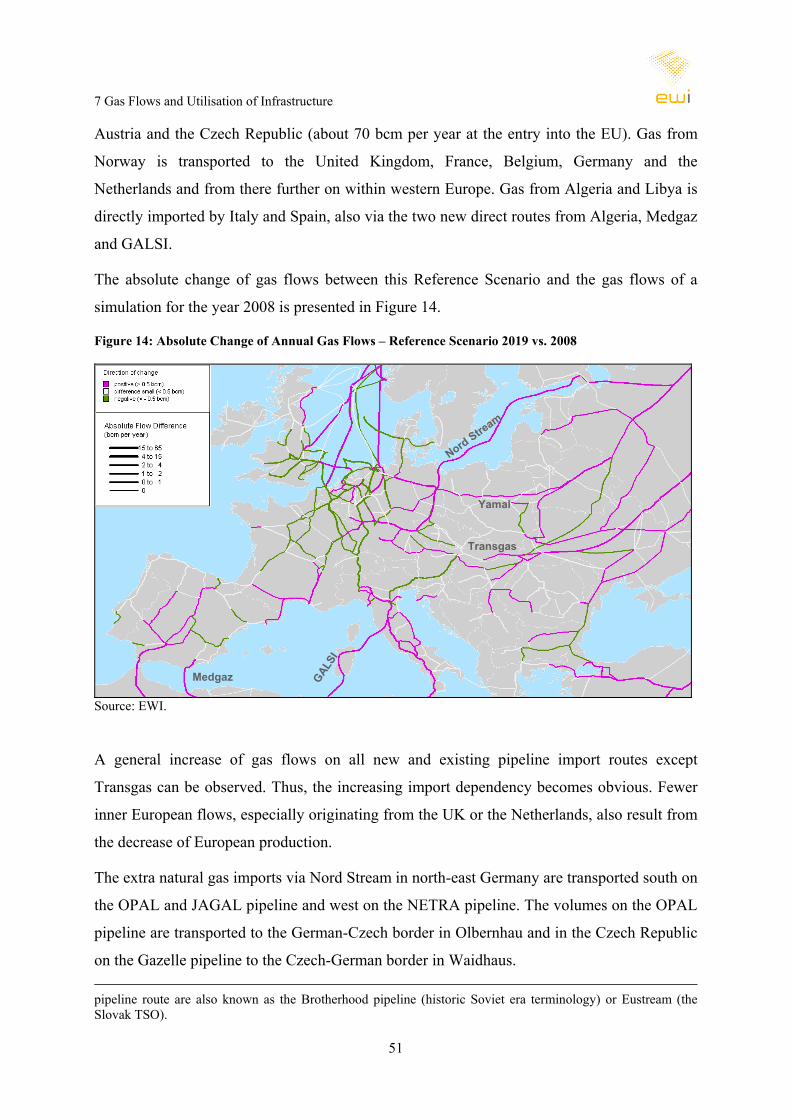
7 Gas Flows and Utilisation of Infrastructure
51
Austria and the Czech Republic (about 70 bcm per year at the entry into the EU). Gas from
Norway is transported to the United Kingdom, France, Belgium, Germany and the
Netherlands and from there further on within western Europe. Gas from Algeria and Libya is
directly imported by Italy and Spain, also via the two new direct routes from Algeria, Medgaz
and GALSI.
The absolute change of gas flows between this Reference Scenario and the gas flows of a
simulation for the year 2008 is presented in Figure 14.
Figure 14: Absolute Change of Annual Gas Flows – Reference Scenario 2019 vs. 2008
Yamal
Nord Stream
GALSI
Medgaz
Transgas
Source: EWI.
A general increase of gas flows on all new and existing pipeline import routes except
Transgas can be observed. Thus, the increasing import dependency becomes obvious. Fewer
inner European flows, especially originating from the UK or the Netherlands, also result from
the decrease of European production.
The extra natural gas imports via Nord Stream in north-east Germany are transported south on
the OPAL and JAGAL pipeline and west on the NETRA pipeline. The volumes on the OPAL
pipeline are transported to the German-Czech border in Olbernhau and in the Czech Republic
on the Gazelle pipeline to the Czech-German border in Waidhaus. pipeline route are also known as the Brotherhood pipeline (historic Soviet era terminology) or Eustream (the Slovak TSO).
7 Gas Flows and Utilisation of Infrastructure
52
The volumes that are imported on the GALSI pipeline via Sardinia reach northern Italy
whereas the volumes on the Transmed45 (Algerian gas) and Greenstream pipeline (gas from
Libya) via Sicily are supplying southern Italy.
Spain also imports pipeline gas (20.8 bcm in 2019) from Algeria via Medgaz and the
Maghreb Europe pipelines. Assuming that there would be a liquid an competitive LNG
market and that this gas could be free and instantaneously diverted between terminals, gas
flows from Spain to France on the MidCat pipeline are only limited (see Section 8.8 for an
extensive discussion). For the year 2019, only slightly more than 1 bcm are transported via
MidCat and only in winter months. Applying the higher ENTSOG demand results in only
minor changes: The main Russian import volumes do not change compared to the same
infrastructure scenario based on the lower EWI/ERGEG demand, but more Russian gas is
transported through Austria to Italy in this case. At the same time, less transit of Russian gas
to France through the MEGAL pipeline takes place. Generally, the higher demand scenario
mirrors the findings of Chaper 1 that an increase in consumption is largely met by additional
LNG imports. Those mainly take place in western Europe. Imports from the north (Norway),
south (Algeria), and east (Russia) are consumed closer to the respective import points in the
EU. Transits of e.g. Russian gas do not reach as far west as in the EWI/ERGEG demand
scenario. (For an illustration of gas flows in the Reference Scenario with ENTSOG demand,
see Figure 58 in the Appendix.)
Nord Stream II Scenario
Implementing the Nord Stream II scenario, simulations with the TIGER model yield the gas
flows shown in Figure 15, Figure 59 and Figure 60 (with the latter two in the Appendix, page
128).
In this scenario more gas is transported via Nord Stream as a second line is in use. After the
Nord Stream landfall, these gas volumes are transported via the onshore connection NEL to
north-west Germany. These volumes substitute gas on the Transgas pipeline where fewer
volumes are transported compared to the Reference Scenario. Transits from Transgas via
Czech Republic to Germany almost fully cease. In addition, less gas volumes are sent through
45 The Transmed pipeline is also sometimes referred to as the Enrico Mattei gas pipeline.
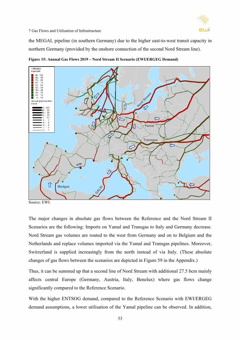
7 Gas Flows and Utilisation of Infrastructure
53
the MEGAL pipeline (in southern Germany) due to the higher east-to-west transit capacity in
northern Germany (provided by the onshore connection of the second Nord Stream line).
Figure 15: Annual Gas Flows 2019 – Nord Stream II Scenario (EWI/ERGEG Demand)
Yamal
Nord Stre
am
GALSIMedgaz
Transgas
Yamal
Nord Stre
am
GALSIMedgaz
Transgas
Source: EWI.
The major changes in absolute gas flows between the Reference and the Nord Stream II
Scenarios are the following: Imports on Yamal and Transgas to Italy and Germany decrease.
Nord Stream gas volumes are routed to the west from Germany and on to Belgium and the
Netherlands and replace volumes imported via the Yamal and Transgas pipelines. Moreover,
Switzerland is supplied increasingly from the north instead of via Italy. (These absolute
changes of gas flows between the scenarios are depicted in Figure 59 in the Appendix.)
Thus, it can be summed up that a second line of Nord Stream with additional 27.5 bcm mainly
affects central Europe (Germany, Austria, Italy, Benelux) where gas flows change
significantly compared to the Reference Scenario.
With the higher ENTSOG demand, compared to the Reference Scenario with EWI/ERGEG
demand assumptions, a lower utilisation of the Yamal pipeline can be observed. In addition,
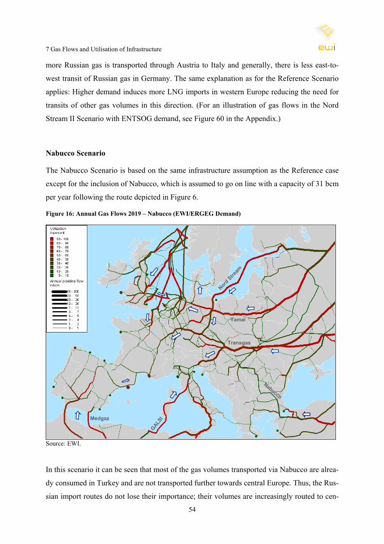
7 Gas Flows and Utilisation of Infrastructure
54
more Russian gas is transported through Austria to Italy and generally, there is less east-to-
west transit of Russian gas in Germany. The same explanation as for the Reference Scenario
applies: Higher demand induces more LNG imports in western Europe reducing the need for
transits of other gas volumes in this direction. (For an illustration of gas flows in the Nord
Stream II Scenario with ENTSOG demand, see Figure 60 in the Appendix.)
Nabucco Scenario
The Nabucco Scenario is based on the same infrastructure assumption as the Reference case
except for the inclusion of Nabucco, which is assumed to go on line with a capacity of 31 bcm
per year following the route depicted in Figure 6.
Figure 16: Annual Gas Flows 2019 – Nabucco (EWI/ERGEG Demand)
Yamal
Nord Stre
am
GALSIMedgaz
Nabucco
Transgas
Yamal
Nord Stre
am
GALSIMedgaz
Nabucco
Transgas
Source: EWI.
In this scenario it can be seen that most of the gas volumes transported via Nabucco are alrea-
dy consumed in Turkey and are not transported further towards central Europe. Thus, the Rus-
sian import routes do not lose their importance; their volumes are increasingly routed to cen-

7 Gas Flows and Utilisation of Infrastructure
55
tral and western Europe. A general increase in east-to-west transits on various pipelines can
be seen. The reasons are the following: Nabucco basically replaces Russian gas volumes in
south-eastern Europe such as Blue Stream volumes and gas imports via Romania. This has
indirect effects in western Europe as less Russian gas is transported to the south-east and more
to central and western Europe. Therefore, Transgas flows increase towards Germany, Italy,
and France. In general, it can be concluded that Nabucco causes Russian pipeline gas volumes
being transported further to the west.
Although gas volumes on Nabucco to Hungary increase in the higher ENTSOG demand
scenario, hardly any volumes from Nabucco would physically be delivered to Baumgarten (as
they could be efficiently swapped with Russian gas along the way). Relative to EWI/ERGEG
demand, Russian gas volumes remain further in the east so that east-to-west transits in central
Europe are even slightly lower. (See Figure 62 in the Appendix for the gas flows based on
ENTSOG demand.)
South Stream Scenario
For the South Stream Scenario, South Stream is included in the infrastructure assumption
instead of Nabucco with a capacity of 63 bcm per year. Its route is presented in Figure 6. To
see the effects of including and excluding the MidCat Pipeline going from Spain to France
(Eastern Axis), and as it is assumed that the inclusion of South Stream has only minor or no
effects on Spain, MidCat is included in all infrastructure scenarios except for the South
Stream Scenario to allow a comparison relative to the Reference case.
The gas flows for this scenario are presented in Figure 17 for the EWI/ERGEG demand (and
in Figure 64 in the Appendix for the ENTSOG demand scenario). The absolute change of an-
nual gas flows for the South Stream Scenario compared to the Reference Scenario is shown in
Figure 61.
Significant gas volumes are imported on South Stream, of which a large share goes to Italy.
Thus, less Russian gas volumes are transited via Slovakia to Austria and on to Italy.
Consequently, fewer volumes are transported to Europe via the Transgas pipeline compared to
the Reference Scenario and less gas is imported via Nord Stream and the Yamal pipeline.
Particularly, this happens due to the fact that South Stream replaces some of the volumes for
Italy, Croatia and Slovenia which are sent through Transgas in the Reference Scenario.

7 Gas Flows and Utilisation of Infrastructure
56
Moreover, Switzerland is supplied to an increasing extent from the south (and less from the
north) when South Stream increases the availability of Russian gas there.
Figure 17: Annual Gas Flows 2019 – South Stream Scenario (EWI/ERGEG Demand)
Yamal
Nord Stre
am
GALSIMedgaz
South Stream
Transgas
Yamal
Nord Stre
am
GALSIMedgaz
South Stream
Transgas
Source: EWI.
The analysis of the effect of the MidCat pipeline is supported by Figure 63. As the MidCat
pipeline is excluded in this scenario, considering the difference of gas flows compared to the
Reference Scenario depicts a reduction on the MidCat pipeline. However, without MidCat,
physical gas flows between Spain and France increase on the Larrau pipeline on the Western
Axis. Thus, these volumes are exported from Spain to France on the Larrau pipeline if the
MidCat pipeline is not available.
Considering the ENTSOG demand scenario and, again, comparing it to the Reference and
EWI/ERGEG demand scenario (see Figure 64 in the Appendix) yields that even more Russian
gas is transported via Austria to Italy. Consequently, less volumes are transported through the
Transgas pipeline and slightly less gas is transported via Nord Stream as north-western
Europe increases its LNG imports in the higher demand scenario.
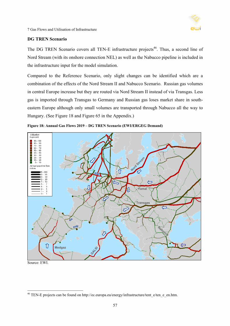
7 Gas Flows and Utilisation of Infrastructure
57
DG TREN Scenario
The DG TREN Scenario covers all TEN-E infrastructure projects46. Thus, a second line of
Nord Stream (with its onshore connection NEL) as well as the Nabucco pipeline is included in
the infrastructure input for the model simulation.
Compared to the Reference Scenario, only slight changes can be identified which are a
combination of the effects of the Nord Stream II and Nabucco Scenario. Russian gas volumes
in central Europe increase but they are routed via Nord Stream II instead of via Transgas. Less
gas is imported through Transgas to Germany and Russian gas loses market share in south-
eastern Europe although only small volumes are transported through Nabucco all the way to
Hungary. (See Figure 18 and Figure 65 in the Appendix.)
Figure 18: Annual Gas Flows 2019 – DG TREN Scenario (EWI/ERGEG Demand)
Yamal
Nord Stre
am
GALSIMedgaz
Nabucco
Transgas
Yamal
Nord Stre
am
GALSIMedgaz
Nabucco
Transgas
Source: EWI.
46 TEN-E projects can be found on http://ec.europa.eu/energy/infrastructure/tent_e/ten_e_en.htm.

7 Gas Flows and Utilisation of Infrastructure
58
Assuming the higher ENTSOG demand (see Figure 66 and Figure 67 in the Appendix)
volumes through Nabucco are increasing (especially on the section from Bulgaria to Hungary)
compared to the EWI/ERGEG demand scenario and more gas is transited via Austria to Italy.
Based on the higher ENTSOG demand, generally, fewer transits further to the (north-)west
take place as demand is higher in eastern Europe in this scenario and gas is already consumed
there. To supply the higher demand in the west, more LNG is imported in Spain, France, and
UK. (The regasification terminals (colored spots) are much higher utilised in Figure 66 than in
Figure 18.) The consequence of the increased LNG imports is a reduction of pipeline imports
to the UK. In addition, more gas is exported from Spain to France. Another effect is that
Norwegian is gas pushed further east from the UK and France to Belgium and Germany and
replaces some Russian gas whereas Russian gas is routed to a larger extent towards Italy or it
is consumed in eastern Europe. (See Figure 66 and Figure 67 in the Appendix.)
LNG Glut Scenario
The LNG Glut Scenario has the intention to analyse the effect of (temporary) low LNG prices
on gas flows in Europe within the modelling framework of TIGER. Hence, LNG volumes are
assumed to be available at very low costs in this scenario (see Section 4.1).
LNG imports rise significantly in every country and especially in the major LNG importing
countries Spain, France and UK. (See Figure 12 for the LNG import volumes and Figure 19
and Figure 69 for the utilisation of the terminals.)
In comparison to the other scenarios, the terminals in northern France and the UK are much
higher utilised as well as the pipelines from these terminals. Furthermore, a high utilisation of
the pipeline from the Krk terminal in Croatia becomes evident. (See Figure 19 and Figure 69.)
In this case, no gas is transported via Nord Stream47 and Yamal and Transgas are only utilised
to a low degree. Pipelines in France and Spain are highly utilised. More gas is exported from
Spain to France on the MidCat pipeline, especially in the winter months.
47 In this specific LNG Glut scenario, all Nord Stream volumes are crowded-out. This is based on the assumption that all gas volumes in take-or-pay contracts can be reduced to zero, which is rather unrealistic to this extent. However, the intention of the LNG Glut simulation was to analyse the effects of this extreme scenario more in qualitative terms showing that low LNG costs in the LNG Glut Scenario might reduce pipeline imports as much as they can flexibly be withheld.
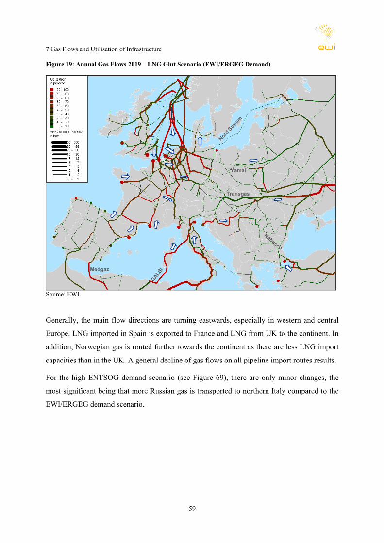
7 Gas Flows and Utilisation of Infrastructure
59
Figure 19: Annual Gas Flows 2019 – LNG Glut Scenario (EWI/ERGEG Demand)
Yamal
Nord Stre
am
GALSIMedgaz
Nabucco
Transgas
Source: EWI.
Generally, the main flow directions are turning eastwards, especially in western and central
Europe. LNG imported in Spain is exported to France and LNG from UK to the continent. In
addition, Norwegian gas is routed further towards the continent as there are less LNG import
capacities than in the UK. A general decline of gas flows on all pipeline import routes results.
For the high ENTSOG demand scenario (see Figure 69), there are only minor changes, the
most significant being that more Russian gas is transported to northern Italy compared to the
EWI/ERGEG demand scenario.
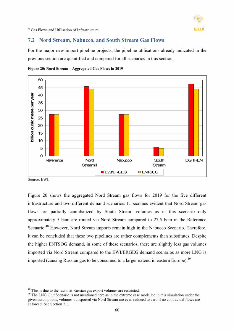
7 Gas Flows and Utilisation of Infrastructure
60
7.2 Nord Stream, Nabucco, and South Stream Gas Flows
For the major new import pipeline projects, the pipeline utilisations already indicated in the
previous section are quantified and compared for all scenarios in this section.
Figure 20: Nord Stream – Aggregated Gas Flows in 2019
0
5
10
15
20
25
30
35
40
45
50
Reference NordStream II
Nabucco SouthStream
DG TREN
EWI/ERGEG ENTSOG
billi
on c
ubic
met
re p
er y
ear
Source: EWI.
Figure 20 shows the aggregated Nord Stream gas flows for 2019 for the five different
infrastructure and two different demand scenarios. It becomes evident that Nord Stream gas
flows are partially cannibalized by South Stream volumes as in this scenario only
approximately 5 bcm are routed via Nord Stream compared to 27.5 bcm in the Reference
Scenario.48 However, Nord Stream imports remain high in the Nabucco Scenario. Therefore,
it can be concluded that these two pipelines are rather complements than substitutes. Despite
the higher ENTSOG demand, in some of these scenarios, there are slightly less gas volumes
imported via Nord Stream compared to the EWI/ERGEG demand scenarios as more LNG is
imported (causing Russian gas to be consumed to a larger extend in eastern Europe).49
48 This is due to the fact that Russian gas export volumes are restricted. 49 The LNG Glut Scenario is not mentioned here as in the extreme case modelled in this simulation under the given assumptions, volumes transported via Nord Stream are even reduced to zero if no contractual flows are enforced. See Section 7.1.
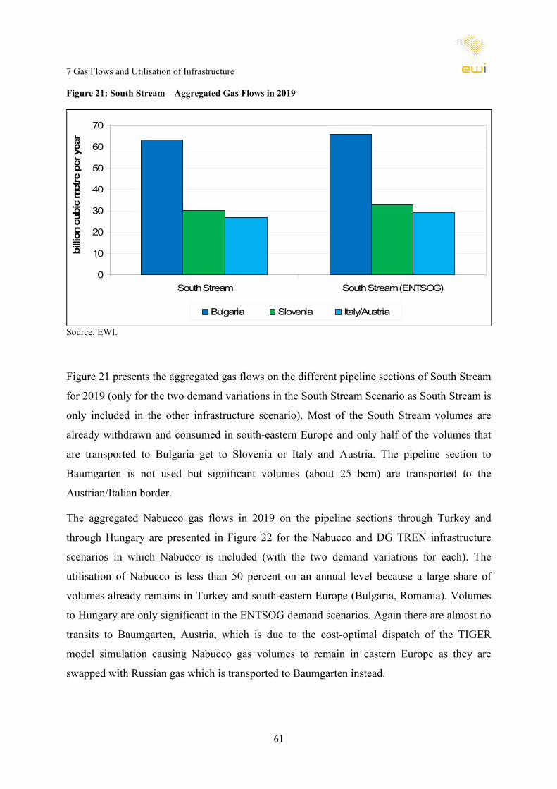
7 Gas Flows and Utilisation of Infrastructure
61
Figure 21: South Stream – Aggregated Gas Flows in 2019
0
10
20
30
40
50
60
70
South Stream South Stream (ENTSOG)
Bulgaria Slovenia Italy/Austria
billi
on c
ubic
met
re p
er y
ear
Source: EWI.
Figure 21 presents the aggregated gas flows on the different pipeline sections of South Stream
for 2019 (only for the two demand variations in the South Stream Scenario as South Stream is
only included in the other infrastructure scenario). Most of the South Stream volumes are
already withdrawn and consumed in south-eastern Europe and only half of the volumes that
are transported to Bulgaria get to Slovenia or Italy and Austria. The pipeline section to
Baumgarten is not used but significant volumes (about 25 bcm) are transported to the
Austrian/Italian border.
The aggregated Nabucco gas flows in 2019 on the pipeline sections through Turkey and
through Hungary are presented in Figure 22 for the Nabucco and DG TREN infrastructure
scenarios in which Nabucco is included (with the two demand variations for each). The
utilisation of Nabucco is less than 50 percent on an annual level because a large share of
volumes already remains in Turkey and south-eastern Europe (Bulgaria, Romania). Volumes
to Hungary are only significant in the ENTSOG demand scenarios. Again there are almost no
transits to Baumgarten, Austria, which is due to the cost-optimal dispatch of the TIGER
model simulation causing Nabucco gas volumes to remain in eastern Europe as they are
swapped with Russian gas which is transported to Baumgarten instead.
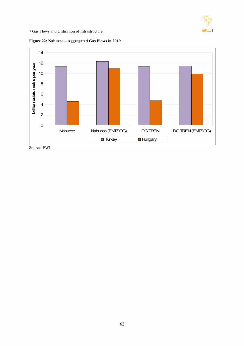
7 Gas Flows and Utilisation of Infrastructure
62
Figure 22: Nabucco – Aggregated Gas Flows in 2019
0
2
4
6
8
10
12
14
Nabucco Nabucco (ENTSOG) DG TREN DG TREN (ENTSOG)
Turkey Hungary
billi
on c
ubic
met
re p
er y
ear
Source: EWI.
8 Market Integration
63
8 Market Integration This chapter analyses physical market integration between the natural gas markets in the
different EU member states with respect to the location of potential bottlenecks and their
implications on security of supply in 2019. In order to assess the integration of the natural gas
markets in the different countries, market integration is initially defined.
8.1 Specification of Market Integration
Generally, the economic literature considers an integrated market as one where there are no
impediments to trade, where all arbitrage opportunities within the market can be exploited and
where, consequently, the Law of One Price holds meaning there are no price differences with-
in the market (provided the good can be supplied to all locations within the market at the same
costs).50 Hence, the possibility to trade is an important prerequisite. Barriers to trade can
thereby stem from taxation (import or export duties), high transaction costs or physical limits
to trade. If none of these impediments to trade is in place, prices in a market would correlate
perfectly.
However, natural gas is not an example for such a market. It is a grid-bound commodity and
transports costs are also a significant proportion of its price.51 Even without any physical li-
mits to trade, prices would, hence, differ between European countries in an efficient market.
As natural gas is a grid-bound commodity, trade is also highly dependent on the availability
of the infrastructure to transport it (from the market with low to the market with the higher
price).
In the context of an analysis of the natural gas infrastructure, the model-based approach
applied in this study is suitable to investigate this physical market integration, i.e. whether the
gas infrastructure provides the prerequisites for an integrated European natural gas market.
Other dimensions of market integration, especially those concerning transaction costs, are not
considered. High transaction costs might, for example, arise from non-harmonised market
regimes, different capacity allocation methods or illiquid natural gas trading. If such issues
complicate trading for market players and increase its costs, the European natural gas market
50 See Baulch (1997) and De Vany and Walls (1996) for discussions on price convergence and market integra-tion, also in the context of natural gas markets (De Vany and Walls, 1996). 51 According to the assumptions applied in the model (see Section 3), transports costs are 1.36 EUR/MWh/1000 kilometres, which equals about 15 percent of the presumed border price for Russian gas imports (see Table 1).
8 Market Integration
64
may still not be integrated, even if the analysis in this study finds parts of the gas market to be
well integrated physically.
The approach applied to investigate market integration in this study is based on price
convergence in integrated markets: The location- and time-specific marginal supply costs
computed by the model can be interpreted as price indicators under the assumptions of a
competitive European gas market with an efficient capacity allocation method. Selecting
representative nodes provides a price estimator for each country and each model time period
and, thus, the differences of marginal supply costs between countries.
In a competitive market, as simulated by the model, this price (represented by marginal
supply cost) difference should always be lower than the transport costs between the
considered countries, i.e. the price difference should lie within the parity bound determined by
transport costs.52 (Transport costs in the model are based on the assumed variable transport
costs and length of the transportation route.) If it were not and physical transport capacity
were still available, traders in a functioning market would always continue to move gas from
the low to the high price location to profit from arbitrage. Hence, in the simulated competitive
market, any price differences exceeding transport costs can only be a consequence of a
physical infrastructure bottleneck which, at least temporarily, leads to a non-integrated
market.
When interpreting the results presented in the next sections, four important points need to be
kept in mind: First, while a bottleneck may hamper competition and limit physical market
integration, it is not necessarily efficient from an economic point of view to eliminate each
bottleneck as the costs of the required investments might exceed the cost of the restriction.
Second, due to the interdependencies between all elements in the gas supply infrastructure, a
seasonal bottleneck in transportation might not be most efficiently removed by investment in
transport capacity; it might be more efficient to invest in storage or LNG regasification
terminals instead.53 In addition, there might be other reasons to consider an investment
necessary such as enhancing security of supply or fostering competition by providing
sufficient capacities. Fourth, the analysis of congestion focuses on bottlenecks between
countries. Although the applied model allows an investigation of bottlenecks within countries,
for a parameterisation in 2019 this would require an elaborate specification of natural gas
52 Parity bound implies that a price difference below this threshold means the market is still integrated, see Baulch (1997). 53 See Lochner (2009).
8 Market Integration
65
demand developments on a regional level, which is not the focus of this study. Therefore,
potential bottlenecks which may arise between balancing areas inside a single country under
certain scenarios are not discussed. With respect to conclusions on potential investment
requirements, this implies that further bottlenecks, which do not cause supply-demand gaps
but which may be needed to ensure high physical market integration within market areas or
individual TSO networks, might additionally arise and warrant investment.
Hence, the bottlenecks identified in this study merely indicate (temporary) impediments to
price convergence (and physical market integration) between countries; they do not imply that
additional investments to remove these bottlenecks are necessarily efficient from an economic
perspective. They are limited to the congestion which occurs in an efficiently working market;
potential additional congestion as a consequence of inefficiencies is not detected by the model
approach. To derive a conclusion on whether a bottleneck should be removed by additional
investment or not, it would be necessary to compare the economic gains from such an
investment (reduced economic cost of the bottleneck) with the monetary size of the
investment necessary to do so (i.e. capital expenditure for new pipeline or interconnector).
Only if the economic gains exceed the costs, it would be beneficial to make the investment.
Analysing this is beyond the scope of this study.
Moreover, as explained in Section 3.1, the bottlenecks presented here do not cover potential
congestion that might originate from inefficient capacity allocation or congestion
management.
8.2 Overview of Bottlenecks
As the following sections provide an in-depth analysis of each identified bottleneck, we first
consider an overview of all combinations of countries considered. Generally, each European
country is investigated for market integration with all its neighbouring countries
individually.54 For each of the six scenarios, an average winter day with demand according to
both, EWI/ERGEG and ENTSOG, an average summer day with EWI/ERGEG demand, and
the peak demand day (ENTSOG assumption) are considered. The results are presented in
Table 4.55 White fields in the matrix imply no bottlenecks between the countries in the
respective scenario on the respective day; a coloured field indicates there is one. The colours,
54 Except for neighbouring countries where no pipeline link either exists or is being planned, e.g. Italy and France. 55 See Table 8 (page 119) for an overview of the used ISO country codes.

8 Market Integration
66
thereby, indicate the type of day. Although it may be clear in most cases, it has to be noted
that Table 4 does not indicate the direction of the bottleneck between the countries, as it may
differ between scenarios and as there is no predominant flow direction for some combination
of countries.
Table 4: Overview Market Integration (Location of Bottlenecks)
Reference Nord Stream II Nabucco South Stream DG TREN LNG Glut
Countries
Win
ter
Sum
mer
Win
ter (
ENTS
OG
)
Peak
Dem
and
Day
Win
ter
Sum
mer
Win
ter (
ENTS
OG
)
Peak
Dem
and
Day
Win
ter
Sum
mer
Win
ter (
ENTS
OG
)
Peak
Dem
and
Day
Win
ter
Sum
mer
Win
ter (
ENTS
OG
)
Peak
Dem
and
Day
Win
ter
Sum
mer
Win
ter (
ENTS
OG
)
Peak
Dem
and
Day
Win
ter
Sum
mer
Win
ter (
ENTS
OG
)
Peak
Dem
and
Day
ES and PTES and FRGB and IEGB and BEGB and NLBE and NLFR and BEDE and NLDE and BEDE and FRCH and DEFR and CHCH and ITDE and DKDE and PLCZ and DE-S*CZ and DE-E*AT and DEAT and ITAT and SIIT and SIHR and SIHR and HUAT and HUHU and ROAT and SKCZ and SKBG and ROBG and GRBG and TRGR and TRGR and IT*Czech border with south (Waidhaus) and east Germany (Olbernhau) respectivelyNote that table does not indicate direction of bottlenecks, see subsequent sections and figures.
No BottleneckBottleneck on average winter day (EWI/ERGEG) Bottleneck on average winter day (ENTSOG)Bottleneck on average summer day (EWI/ERGEG) Bottleneck on peak demand day (ENTSOG)
Source: EWI.
For the Reference and LNG Glut scenarios, Figure 23 and Figure 24 visualise the identified
bottlenecks on the respective days with the arrows pointing into the direction of the
bottleneck. (For the other four scenarios, these charts can be found in the Appendix.)
Furthermore, details on all identified bottlenecks (including their direction) are discussed in
the subsequent sections.

8 Market Integration
67
Figure 23: Bottlenecks Reference Scenario 2019
Bottleneck in direction of arrow on:
Winter DaySummer DayWinter (ENTSOG)
Peak day
Source: EWI.
Generally, it can be noted that most European countries are well integrated on the average
winter and summer days (in all scenarios and with both demand assumptions). The only
persistent bottleneck is between Germany and Denmark. In 2019, according to the applied
ENTSOG demand and supply scenarios, Danish (and Swedish) consumption cannot be met by
the assumed existing import capacity and Danish production. Hence, large price increases in
Denmark would be observed implying a large marginal supply cost difference to Germany
and demand for additional capacity between the countries.
In eastern Europe, some bottlenecks are identified between Hungary, Slovenia and the Slovak
Republic and some of their neighbouring countries. While the costs of these bottlenecks differ
significantly (see Section 8.3), they can generally be observed in winter in both demand
scenarios and on the peak days. However, it also has to be noted that the large-scale
infrastructure projects in south-eastern Europe, Nabucco and South Stream, help to eliminate
some of these bottlenecks.

8 Market Integration
68
Figure 24: Bottlenecks LNG Glut Scenario 2019
Bottleneck in direction of arrow on:
Winter DaySummer DayWinter (ENTSOG)
Peak day
Source: EWI.
In the region of western Europe, bottlenecks between some of the countries arise in the
simulation, but only on the concurrent peak day and in times of low LNG prices. On the
concurrent peak demand day, there are bottlenecks between the region of France, Belgium
and the Netherlands and all its surrounding neighbours. In between this group of countries,
the market seems to be well integrated physically. In times of low LNG prices, the model
finds that more LNG could be transported from the LNG import capacities in the west further
to the east if more capacity were available. Specifically, bottlenecks between the UK and the
continent, France and all its eastern neighbours and the Benelux countries and Germany are
identified. (Similar issues arise from the Croatian Krk LNG terminal to neighbouring
countries when LNG prices are low.)
In the following sections, all these bottlenecks are discussed in detail. The detailed graphs of
the country combinations without bottlenecks (see Table 4), which are omitted in the
following sections, can be found in Appendix (starting page 136). An explanation of the
graphs is also illustrated in Figure 70 (page 134).

8 Market Integration
69
8.3 Eastern Europe: Hungary, Slovak Republic and neighbouring countries
The bottlenecks regarding Hungary and the Slovak Republic indicated in Table 4 are found to
differ significantly when investigated in detail.
Regarding the Slovak Republic, the costs of the bottleneck (difference in country-specific
marginal supply costs in excess of transport costs56) to the Czech Republic is small, as can be
seen in Figure 25 and can largely be explained by bottlenecks within the Czech grid.57
Figure 25: Marginal Supply Cost Difference between the Czech and Slovak Republics
0.00
0.05
0.10
0.15
0.20
0.25
0.30
0.35
0.40
0.45
0.50
Win
ter
Sum
mer
Win
ter(E
NTS
OG
)
Pea
k D
ay
Win
ter
Sum
mer
Win
ter(E
NTS
OG
)
Pea
k D
ay
Win
ter
Sum
mer
Win
ter(E
NTS
OG
)
Pea
k D
ay
Win
ter
Sum
mer
Win
ter(E
NTS
OG
)
Pea
k D
ay
Win
ter
Sum
mer
Win
ter(E
NTS
OG
)
Pea
k D
ay
Win
ter
Sum
mer
Win
ter(E
NTS
OG
)
Pea
k D
ay
Reference Nord Stream II Nabucco South Stream DG TREN LNG Glut
EUR
/ M
Wh
Source: EWI.
For the connection from the Slovak Republic to Baumgarten, Austria (Figure 26), the
economic costs of the bottleneck are higher in times of high demand, i.e. on the peak demand
day or in winter with the higher ENTSOG-demand. In these cases more Russian gas could be
transported via Slovakia to Austria (and further west) if more capacity on the route were
56 See Figure 70 (page 134) for an illustration of the interpretation of the following charts. Generally, the bars indicate the supply cost difference between the countries (first named country in caption minus second stated country); the dotted line represents the transport costs between those countries. If the cost difference exceeds the transport costs, further arbitrage would be beneficial but cannot take place (which would lead to a smaller cost difference) as there is not sufficient capacity available. Hence, there must be a physical bottleneck. The colours of the bars only indicate the type of day (corresponding to the colours in Table 4): Winter day EWI/ERGEG in light blue, summer day in Navajo white, winter day ENTSOG in blue, and peak demand day in dark magenta. 57 A representative location in the centre of the Czech Republic was chosen as a reference.

8 Market Integration
70
available. This is generally possible in all scenarios after 2012 when the first line of Nord
Stream is completed and, hence, less Russian gas via Slovakia is transported towards
Germany freeing up capacity on this route for gas transports to Austria and Italy. While the
interconnection between Slovakia and Austria is always highly utilised, it only constitutes a
bottleneck in times of high demand (peak day or winter with ENTSOG demand). When South
Stream is in place as a second transport route for Russian gas to Austria and Italy, this
bottleneck disappears even in times of higher demand.
Figure 26: Marginal Supply Cost Difference between Austria and the Slovak Republic
0.00
0.10
0.20
0.30
0.40
0.50
0.60
0.70
0.80
0.90
1.00
Win
ter
Sum
mer
Win
ter(E
NTS
OG
)
Pea
k D
ay
Win
ter
Sum
mer
Win
ter(E
NTS
OG
)
Pea
k D
ay
Win
ter
Sum
mer
Win
ter(E
NTS
OG
)
Pea
k D
ay
Win
ter
Sum
mer
Win
ter(E
NTS
OG
)
Pea
k D
ay
Win
ter
Sum
mer
Win
ter(E
NTS
OG
)
Pea
k D
ay
Win
ter
Sum
mer
Win
ter(E
NTS
OG
)
Pea
k D
ay
Reference Nord Stream II Nabucco South Stream DG TREN LNG Glut
EUR
/ M
Wh
Source: EWI.
The case is generally different for the bottlenecks between Hungary and the surrounding
countries, see Figure 27 and Figure 28. In the scenarios without South Stream or Nabucco,
which both provide new import capacity to Hungary,58 demand on peak days or on winter
days with higher demand (ENTSOG demand scenario) cannot be met and the marginal supply
costs increase significantly. (For a discussion of the supply-demand gaps and security of
supply implications arising from the bottlenecks, see Section 8.10 on page 91.) Hence, the
cost of the bottleneck, or the economic value of additional capacity, between Hungary and
both, Austria (Figure 27) and Romania (Figure 28), increases significantly. In the summer
58 Nabucco directly and South Stream has exit points in Serbia which is relatively well connected with the Hun-garian grid.

8 Market Integration
71
months, and in scenarios with either South Stream or Nabucco, market integration of Hungary
and the neighbouring countries is, however, less of an issue.
Figure 27: Marginal Supply Cost Difference between Hungary and Austria
-1.00
0.00
1.00
2.00
3.00
4.00
5.00
6.00
7.00
Win
ter
Sum
mer
Win
ter(E
NTS
OG
)
Pea
k D
ay
Win
ter
Sum
mer
Win
ter(E
NTS
OG
)
Pea
k D
ay
Win
ter
Sum
mer
Win
ter(E
NTS
OG
)
Pea
k D
ay
Win
ter
Sum
mer
Win
ter(E
NTS
OG
)
Pea
k D
ay
Win
ter
Sum
mer
Win
ter(E
NTS
OG
)
Pea
k D
ay
Win
ter
Sum
mer
Win
ter(E
NTS
OG
)
Pea
k D
ay
Reference Nord Stream II Nabucco South Stream DG TREN LNG Glut
EUR
/ M
Wh
Source: EWI.
Figure 28: Marginal Supply Cost Difference between Hungary and Romania
0.00
1.00
2.00
3.00
4.00
5.00
6.00
7.00
8.00
Win
ter
Sum
mer
Win
ter(E
NTS
OG
)
Pea
k D
ay
Win
ter
Sum
mer
Win
ter(E
NTS
OG
)
Pea
k D
ay
Win
ter
Sum
mer
Win
ter(E
NTS
OG
)
Pea
k D
ay
Win
ter
Sum
mer
Win
ter(E
NTS
OG
)
Pea
k D
ay
Win
ter
Sum
mer
Win
ter(E
NTS
OG
)
Pea
k D
ay
Win
ter
Sum
mer
Win
ter(E
NTS
OG
)
Pea
k D
ay
Reference Nord Stream II Nabucco South Stream DG TREN LNG Glut
EUR
/ M
Wh
Source: EWI.
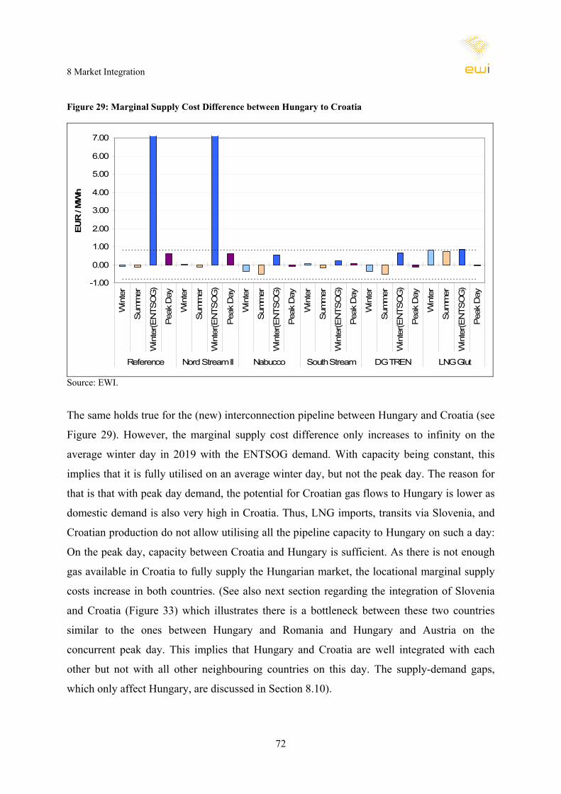
8 Market Integration
72
Figure 29: Marginal Supply Cost Difference between Hungary to Croatia
-1.00
0.00
1.00
2.00
3.00
4.00
5.00
6.00
7.00
Win
ter
Sum
mer
Win
ter(E
NTS
OG
)
Pea
k D
ay
Win
ter
Sum
mer
Win
ter(E
NTS
OG
)
Pea
k D
ay
Win
ter
Sum
mer
Win
ter(E
NTS
OG
)
Pea
k D
ay
Win
ter
Sum
mer
Win
ter(E
NTS
OG
)
Pea
k D
ay
Win
ter
Sum
mer
Win
ter(E
NTS
OG
)
Pea
k D
ay
Win
ter
Sum
mer
Win
ter(E
NTS
OG
)
Pea
k D
ay
Reference Nord Stream II Nabucco South Stream DG TREN LNG Glut
EUR
/ M
Wh
Source: EWI.
The same holds true for the (new) interconnection pipeline between Hungary and Croatia (see
Figure 29). However, the marginal supply cost difference only increases to infinity on the
average winter day in 2019 with the ENTSOG demand. With capacity being constant, this
implies that it is fully utilised on an average winter day, but not the peak day. The reason for
that is that with peak day demand, the potential for Croatian gas flows to Hungary is lower as
domestic demand is also very high in Croatia. Thus, LNG imports, transits via Slovenia, and
Croatian production do not allow utilising all the pipeline capacity to Hungary on such a day:
On the peak day, capacity between Croatia and Hungary is sufficient. As there is not enough
gas available in Croatia to fully supply the Hungarian market, the locational marginal supply
costs increase in both countries. (See also next section regarding the integration of Slovenia
and Croatia (Figure 33) which illustrates there is a bottleneck between these two countries
similar to the ones between Hungary and Romania and Hungary and Austria on the
concurrent peak day. This implies that Hungary and Croatia are well integrated with each
other but not with all other neighbouring countries on this day. The supply-demand gaps,
which only affect Hungary, are discussed in Section 8.10).
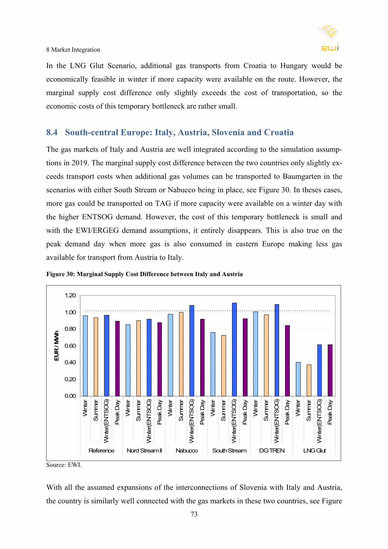
8 Market Integration
73
In the LNG Glut Scenario, additional gas transports from Croatia to Hungary would be
economically feasible in winter if more capacity were available on the route. However, the
marginal supply cost difference only slightly exceeds the cost of transportation, so the
economic costs of this temporary bottleneck are rather small.
8.4 South-central Europe: Italy, Austria, Slovenia and Croatia
The gas markets of Italy and Austria are well integrated according to the simulation assump-
tions in 2019. The marginal supply cost difference between the two countries only slightly ex-
ceeds transport costs when additional gas volumes can be transported to Baumgarten in the
scenarios with either South Stream or Nabucco being in place, see Figure 30. In theses cases,
more gas could be transported on TAG if more capacity were available on a winter day with
the higher ENTSOG demand. However, the cost of this temporary bottleneck is small and
with the EWI/ERGEG demand assumptions, it entirely disappears. This is also true on the
peak demand day when more gas is also consumed in eastern Europe making less gas
available for transport from Austria to Italy.
Figure 30: Marginal Supply Cost Difference between Italy and Austria
0.00
0.20
0.40
0.60
0.80
1.00
1.20
Win
ter
Sum
mer
Win
ter(E
NTS
OG
)
Pea
k D
ay
Win
ter
Sum
mer
Win
ter(E
NTS
OG
)
Pea
k D
ay
Win
ter
Sum
mer
Win
ter(E
NTS
OG
)
Pea
k D
ay
Win
ter
Sum
mer
Win
ter(E
NTS
OG
)
Pea
k D
ay
Win
ter
Sum
mer
Win
ter(E
NTS
OG
)
Pea
k D
ay
Win
ter
Sum
mer
Win
ter(E
NTS
OG
)
Pea
k D
ay
Reference Nord Stream II Nabucco South Stream DG TREN LNG Glut
EUR
/ M
Wh
Source: EWI.
With all the assumed expansions of the interconnections of Slovenia with Italy and Austria,
the country is similarly well connected with the gas markets in these two countries, see Figure
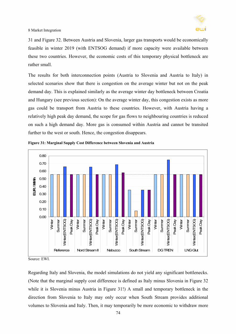
8 Market Integration
74
31 and Figure 32. Between Austria and Slovenia, larger gas transports would be economically
feasible in winter 2019 (with ENTSOG demand) if more capacity were available between
these two countries. However, the economic costs of this temporary physical bottleneck are
rather small.
The results for both interconnection points (Austria to Slovenia and Austria to Italy) in
selected scenarios show that there is congestion on the average winter but not on the peak
demand day. This is explained similarly as the average winter day bottleneck between Croatia
and Hungary (see previous section): On the average winter day, this congestion exists as more
gas could be transport from Austria to these countries. However, with Austria having a
relatively high peak day demand, the scope for gas flows to neighbouring countries is reduced
on such a high demand day. More gas is consumed within Austria and cannot be transited
further to the west or south. Hence, the congestion disappears.
Figure 31: Marginal Supply Cost Difference between Slovenia and Austria
0.00
0.10
0.20
0.30
0.40
0.50
0.60
0.70
0.80
Win
ter
Sum
mer
Win
ter(E
NTS
OG
)
Pea
k D
ay
Win
ter
Sum
mer
Win
ter(E
NTS
OG
)
Pea
k D
ay
Win
ter
Sum
mer
Win
ter(E
NTS
OG
)
Pea
k D
ay
Win
ter
Sum
mer
Win
ter(E
NTS
OG
)
Pea
k D
ay
Win
ter
Sum
mer
Win
ter(E
NTS
OG
)
Pea
k D
ay
Win
ter
Sum
mer
Win
ter(E
NTS
OG
)
Pea
k D
ay
Reference Nord Stream II Nabucco South Stream DG TREN LNG Glut
EUR
/ M
Wh
Source: EWI.
Regarding Italy and Slovenia, the model simulations do not yield any significant bottlenecks.
(Note that the marginal supply cost difference is defined as Italy minus Slovenia in Figure 32
while it is Slovenia minus Austria in Figure 31!) A small and temporary bottleneck in the
direction from Slovenia to Italy may only occur when South Stream provides additional
volumes to Slovenia and Italy. Then, it may temporarily be more economic to withdraw more
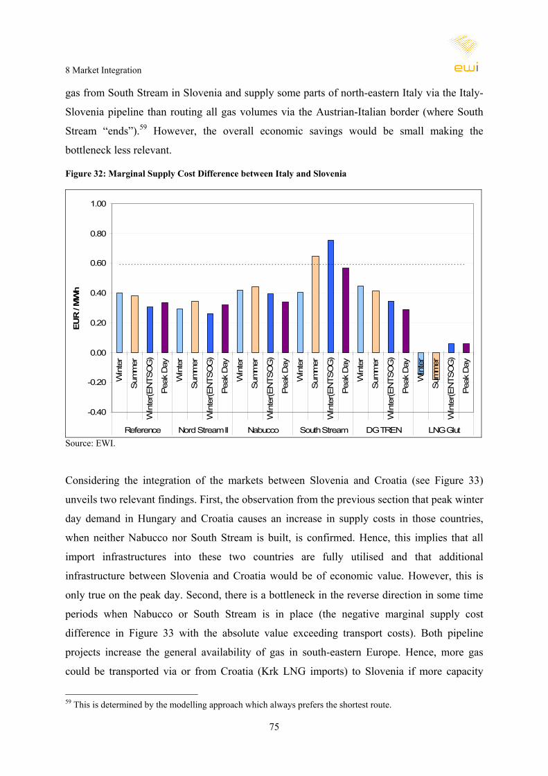
8 Market Integration
75
gas from South Stream in Slovenia and supply some parts of north-eastern Italy via the Italy-
Slovenia pipeline than routing all gas volumes via the Austrian-Italian border (where South
Stream “ends”).59 However, the overall economic savings would be small making the
bottleneck less relevant.
Figure 32: Marginal Supply Cost Difference between Italy and Slovenia
-0.40
-0.20
0.00
0.20
0.40
0.60
0.80
1.00
Win
ter
Sum
mer
Win
ter(E
NTS
OG
)
Pea
k D
ay
Win
ter
Sum
mer
Win
ter(E
NTS
OG
)
Pea
k D
ay
Win
ter
Sum
mer
Win
ter(E
NTS
OG
)
Pea
k D
ay
Win
ter
Sum
mer
Win
ter(E
NTS
OG
)
Pea
k D
ay
Win
ter
Sum
mer
Win
ter(E
NTS
OG
)
Pea
k D
ay
Win
ter
Sum
mer
Win
ter(E
NTS
OG
)
Pea
k D
ay
Reference Nord Stream II Nabucco South Stream DG TREN LNG Glut
EUR
/ M
Wh
Source: EWI.
Considering the integration of the markets between Slovenia and Croatia (see Figure 33)
unveils two relevant findings. First, the observation from the previous section that peak winter
day demand in Hungary and Croatia causes an increase in supply costs in those countries,
when neither Nabucco nor South Stream is built, is confirmed. Hence, this implies that all
import infrastructures into these two countries are fully utilised and that additional
infrastructure between Slovenia and Croatia would be of economic value. However, this is
only true on the peak day. Second, there is a bottleneck in the reverse direction in some time
periods when Nabucco or South Stream is in place (the negative marginal supply cost
difference in Figure 33 with the absolute value exceeding transport costs). Both pipeline
projects increase the general availability of gas in south-eastern Europe. Hence, more gas
could be transported via or from Croatia (Krk LNG imports) to Slovenia if more capacity
59 This is determined by the modelling approach which always prefers the shortest route.

8 Market Integration
76
were available in times of high demand. This is especially severe in times of temporarily low
LNG prices (LNG Glut Scenario) when the limited capacity between Croatia and Slovenia
prevents further LNG imports in Krk for the Slovenia market.
Figure 33: Marginal Supply Cost Difference between Croatia and Slovenia
-2.00
-1.00
0.00
1.00
2.00
3.00
4.00
5.00
6.00
Win
ter
Sum
mer
Win
ter(E
NTS
OG
)
Pea
k D
ay
Win
ter
Sum
mer
Win
ter(E
NTS
OG
)
Pea
k D
ay
Win
ter
Sum
mer
Win
ter(E
NTS
OG
)
Pea
k D
ay
Win
ter
Sum
mer
Win
ter(E
NTS
OG
)
Pea
k D
ay
Win
ter
Sum
mer
Win
ter(E
NTS
OG
)
Pea
k D
ay
Win
ter
Sum
mer
Win
ter(E
NTS
OG
)
Pea
k D
ay
Reference Nord Stream II Nabucco South Stream DG TREN LNG Glut
EUR
/ M
Wh
Source: EWI.
8.5 Central Europe: Germany and neighbouring countries
Regarding the market integration of Germany with its neighbouring countries, Table 4 illus-
trates that there is a persistent bottleneck to Denmark and some temporary bottlenecks with its
western neighbours and the Czech Republic. The integration to the west is discussed in Sec-
tion 8.7 and with Denmark in Section 8.6. For the countries where no bottlenecks to Germany
exist, the respective charts can be retrieved in the Appendix: Austria (Figure 77), Switzerland
(Figure 78) and Poland (Figure 80).
The gas flow analyses in Section 7.1 have shown that in 2019, natural gas imports on Nord
Stream in north-eastern Germany are (partially) transported south on the OPAL pipeline to the
German-Czech border in Olbernhau and in the Czech Republic on the Gazelle pipeline to the
Czech-German border in Waidhaus. Hence, the gas volumes exit Germany to the Czech
Republic in eastern Germany and re-enter southern Germany from the Czech Republic. This
requires the analysis of two potential bottlenecks. The marginal supply cost differences
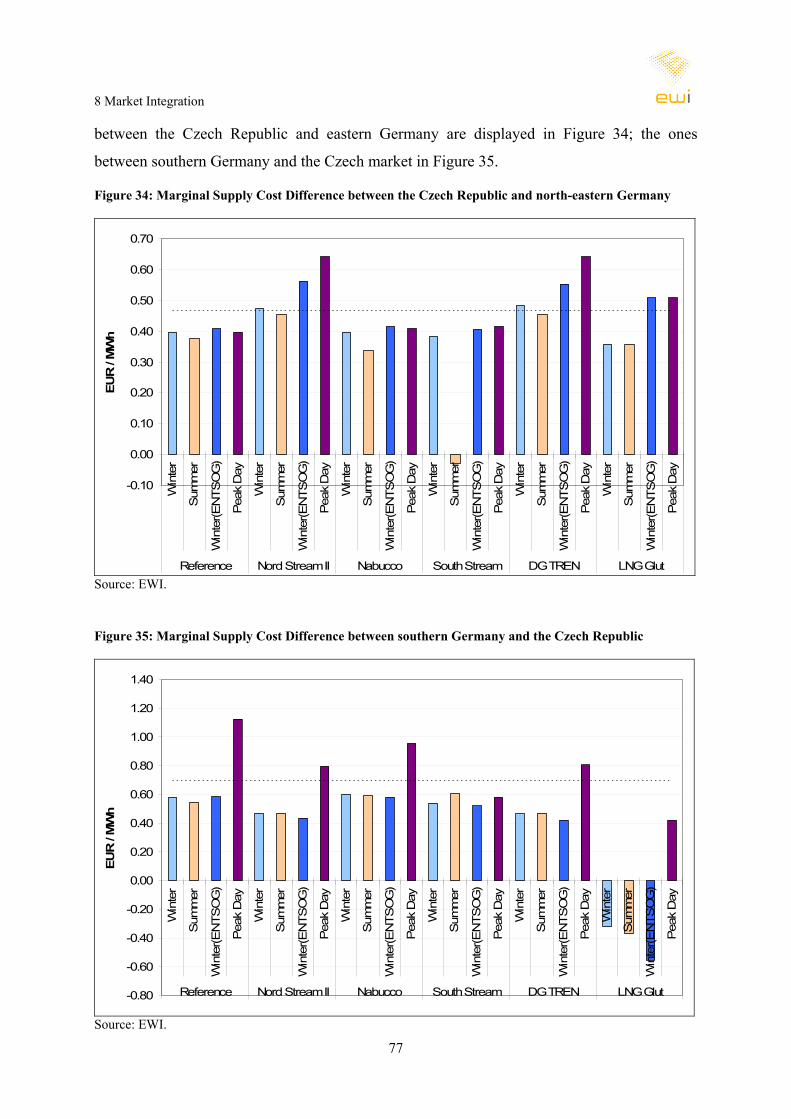
8 Market Integration
77
between the Czech Republic and eastern Germany are displayed in Figure 34; the ones
between southern Germany and the Czech market in Figure 35.
Figure 34: Marginal Supply Cost Difference between the Czech Republic and north-eastern Germany
-0.10
0.00
0.10
0.20
0.30
0.40
0.50
0.60
0.70
Win
ter
Sum
mer
Win
ter(E
NTS
OG
)
Pea
k D
ay
Win
ter
Sum
mer
Win
ter(E
NTS
OG
)
Pea
k D
ay
Win
ter
Sum
mer
Win
ter(E
NTS
OG
)
Pea
k D
ay
Win
ter
Sum
mer
Win
ter(E
NTS
OG
)
Pea
k D
ay
Win
ter
Sum
mer
Win
ter(E
NTS
OG
)
Pea
k D
ay
Win
ter
Sum
mer
Win
ter(E
NTS
OG
)
Pea
k D
ay
Reference Nord Stream II Nabucco South Stream DG TREN LNG Glut
EUR
/ M
Wh
Source: EWI.
Figure 35: Marginal Supply Cost Difference between southern Germany and the Czech Republic
-0.80
-0.60
-0.40
-0.20
0.00
0.20
0.40
0.60
0.80
1.00
1.20
1.40
Win
ter
Sum
mer
Win
ter(E
NTS
OG
)
Pea
k D
ay
Win
ter
Sum
mer
Win
ter(E
NTS
OG
)
Pea
k D
ay
Win
ter
Sum
mer
Win
ter(E
NTS
OG
)
Pea
k D
ay
Win
ter
Sum
mer
Win
ter(E
NTS
OG
)
Pea
k D
ay
Win
ter
Sum
mer
Win
ter(E
NTS
OG
)
Pea
k D
ay
Win
ter
Sum
mer
Win
ter(E
NTS
OG
)
Pea
k D
ay
Reference Nord Stream II Nabucco South Stream DG TREN LNG Glut
EUR
/ M
Wh
Source: EWI.

8 Market Integration
78
For the connection from eastern Germany to the Czech Republic (OPAL pipeline), it becomes
evident that capacity is sufficient for one line of the Nord Stream pipeline (scenarios
Reference, Nabucco and South Stream). When a second line of Nord Stream doubles capacity
to 55 bcm/year (scenarios Nord Stream II and DG TREN), there is a temporary bottleneck
between eastern Germany and the Czech Republic in winter as even more gas from Nord
Stream could be transported further to Czech consumers. However, apart from its temporary
nature, the economic costs of the bottleneck are rather small.
Regarding the market integration of southern Germany and the Czech Republic (Figure 35),
there is only a bottleneck on the peak demand day. For all other demand variations, the
capacities in Waidhaus are sufficient to ensure an integration of the Czech and German
markets. It is noteworthy, that the marginal supply cost difference between Germany and the
Czech Republic is negative in the LNG Glut Scenario (except on peak days) implying that
marginal supply costs are higher in the Czech Republic and that gas will actually flow from
the west to the east in this case. However, the absolute marginal supply cost difference does
not exceed transport costs implying that capacity in Waidhaus is sufficient for west-to-east
transport on this route.
8.6 Scandinavia: Denmark and Germany
The case of Denmark is the only bottleneck found to be persistent in all scenarios and across
the whole year 2019 according to our simulations in this study. This is, thereby, largely a
consequence of the assumptions. According to ENTSOG (2009), Danish production declines
to 1.8 bcm in 2019. With Danish and Swedish demand at 5 bcm in 2019,60 the existing import
capacity from Germany is not sufficient to meet demand in the two countries.61 Hence, there
is a significant bottleneck if no other import infrastructures to Denmark are realised. As
potential pipeline projects between Denmark and Norway or across the Baltic Sea to Poland
seem less likely at the moment, this implies a need for increased capacity between Germany
and Denmark to enable gas imports to compensate for declines in Danish production. The
costs of congestion are depicted in Figure 36 and indicate a need for investment.
As for the integration of Sweden and Denmark, this largely depends on natural gas demand
growth in Sweden. If demand grows as projected, and expansion of pipeline link between the
countries may also be required. 60 ENTSOG (2009). Sweden is solely supplied via Denmark in our infrastructure assumptions. 61 According to ENTSOG (2009), capacity is not expanded.

8 Market Integration
79
Figure 36: Marginal Supply Cost Difference between Denmark and Germany
0.00
10.00
20.00
30.00
40.00
50.00
60.00W
inte
r
Sum
mer
Win
ter(E
NTS
OG
)
Pea
k D
ay
Win
ter
Sum
mer
Win
ter(E
NTS
OG
)
Pea
k D
ay
Win
ter
Sum
mer
Win
ter(E
NTS
OG
)
Pea
k D
ay
Win
ter
Sum
mer
Win
ter(E
NTS
OG
)
Pea
k D
ay
Win
ter
Sum
mer
Win
ter(E
NTS
OG
)
Pea
k D
ay
Win
ter
Sum
mer
Win
ter(E
NTS
OG
)
Pea
k D
ay
Reference Nord Stream II Nabucco South Stream DG TREN LNG Glut
EUR
/
Source: EWI.
8.7 Western and Central Europe
Generally, market integration amongst western European countries and between western and
central Europe is fairly advanced. There are hardly any temporary bottlenecks. Nevertheless,
two issues seem to be relevant when investigating these countries: First, there appears to be a
bottleneck on peak days between the region of the Netherlands, Belgium and France and
Great Britain on the one hand and Germany on the other. Second, the LNG Glut scenario is
specially conceived to address issues of market integration in the case of temporarily low
LNG prices, i.e. whether or not there are sufficient transport capacities to make full use of the
LNG import capacities and supply LNG volumes to markets without direct access to LNG
terminals. The analysis shows that some congestion may exist in this case.
Considering the United Kingdom, physical market integration is found to be high in our
model simulations:
• There is no bottleneck to the Irish market (see Figure 75 on page 115 in the Appendix).
• On the Interconnector to Belgium there is only a bottleneck on peak days. Generally, gas
flows in winter (including peak days) go from Britain to the continent (as there are
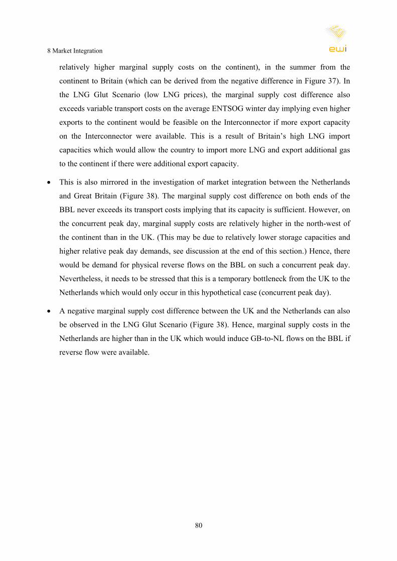
8 Market Integration
80
relatively higher marginal supply costs on the continent), in the summer from the
continent to Britain (which can be derived from the negative difference in Figure 37). In
the LNG Glut Scenario (low LNG prices), the marginal supply cost difference also
exceeds variable transport costs on the average ENTSOG winter day implying even higher
exports to the continent would be feasible on the Interconnector if more export capacity
on the Interconnector were available. This is a result of Britain’s high LNG import
capacities which would allow the country to import more LNG and export additional gas
to the continent if there were additional export capacity.
• This is also mirrored in the investigation of market integration between the Netherlands
and Great Britain (Figure 38). The marginal supply cost difference on both ends of the
BBL never exceeds its transport costs implying that its capacity is sufficient. However, on
the concurrent peak day, marginal supply costs are relatively higher in the north-west of
the continent than in the UK. (This may be due to relatively lower storage capacities and
higher relative peak day demands, see discussion at the end of this section.) Hence, there
would be demand for physical reverse flows on the BBL on such a concurrent peak day.
Nevertheless, it needs to be stressed that this is a temporary bottleneck from the UK to the
Netherlands which would only occur in this hypothetical case (concurrent peak day).
• A negative marginal supply cost difference between the UK and the Netherlands can also
be observed in the LNG Glut Scenario (Figure 38). Hence, marginal supply costs in the
Netherlands are higher than in the UK which would induce GB-to-NL flows on the BBL if
reverse flow were available.
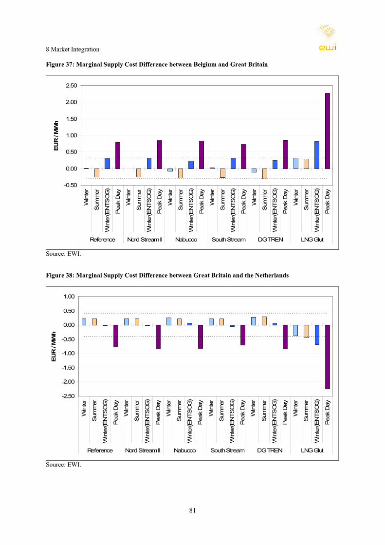
8 Market Integration
81
Figure 37: Marginal Supply Cost Difference between Belgium and Great Britain
-0.50
0.00
0.50
1.00
1.50
2.00
2.50W
inte
r
Sum
mer
Win
ter(E
NTS
OG
)
Pea
k D
ay
Win
ter
Sum
mer
Win
ter(E
NTS
OG
)
Pea
k D
ay
Win
ter
Sum
mer
Win
ter(E
NTS
OG
)
Pea
k D
ay
Win
ter
Sum
mer
Win
ter(E
NTS
OG
)
Pea
k D
ay
Win
ter
Sum
mer
Win
ter(E
NTS
OG
)
Pea
k D
ay
Win
ter
Sum
mer
Win
ter(E
NTS
OG
)
Pea
k D
ay
Reference Nord Stream II Nabucco South Stream DG TREN LNG Glut
EUR
/ M
Wh
Source: EWI.
Figure 38: Marginal Supply Cost Difference between Great Britain and the Netherlands
-2.50
-2.00
-1.50
-1.00
-0.50
0.00
0.50
1.00
Win
ter
Sum
mer
Win
ter(E
NTS
OG
)
Pea
k D
ay
Win
ter
Sum
mer
Win
ter(E
NTS
OG
)
Pea
k D
ay
Win
ter
Sum
mer
Win
ter(E
NTS
OG
)
Pea
k D
ay
Win
ter
Sum
mer
Win
ter(E
NTS
OG
)
Pea
k D
ay
Win
ter
Sum
mer
Win
ter(E
NTS
OG
)
Pea
k D
ay
Win
ter
Sum
mer
Win
ter(E
NTS
OG
)
Pea
k D
ay
Reference Nord Stream II Nabucco South Stream DG TREN LNG Glut
EUR
/ M
Wh
Source: EWI.
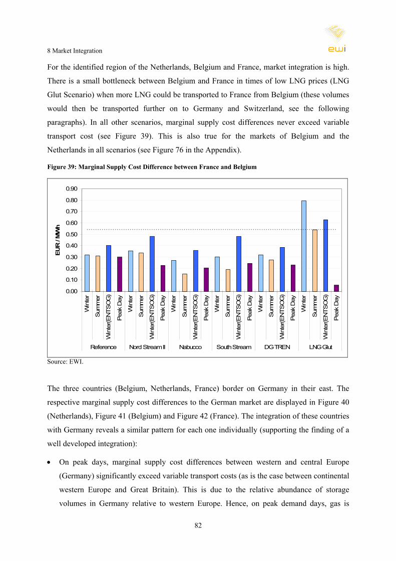
8 Market Integration
82
For the identified region of the Netherlands, Belgium and France, market integration is high.
There is a small bottleneck between Belgium and France in times of low LNG prices (LNG
Glut Scenario) when more LNG could be transported to France from Belgium (these volumes
would then be transported further on to Germany and Switzerland, see the following
paragraphs). In all other scenarios, marginal supply cost differences never exceed variable
transport cost (see Figure 39). This is also true for the markets of Belgium and the
Netherlands in all scenarios (see Figure 76 in the Appendix).
Figure 39: Marginal Supply Cost Difference between France and Belgium
0.00
0.10
0.20
0.30
0.40
0.50
0.60
0.70
0.80
0.90
Win
ter
Sum
mer
Win
ter(E
NTS
OG
)
Pea
k D
ay
Win
ter
Sum
mer
Win
ter(E
NTS
OG
)
Pea
k D
ay
Win
ter
Sum
mer
Win
ter(E
NTS
OG
)
Pea
k D
ay
Win
ter
Sum
mer
Win
ter(E
NTS
OG
)
Pea
k D
ay
Win
ter
Sum
mer
Win
ter(E
NTS
OG
)
Pea
k D
ay
Win
ter
Sum
mer
Win
ter(E
NTS
OG
)
Pea
k D
ay
Reference Nord Stream II Nabucco South Stream DG TREN LNG Glut
EUR
/ M
Wh
Source: EWI.
The three countries (Belgium, Netherlands, France) border on Germany in their east. The
respective marginal supply cost differences to the German market are displayed in Figure 40
(Netherlands), Figure 41 (Belgium) and Figure 42 (France). The integration of these countries
with Germany reveals a similar pattern for each one individually (supporting the finding of a
well developed integration):
• On peak days, marginal supply cost differences between western and central Europe
(Germany) significantly exceed variable transport costs (as is the case between continental
western Europe and Great Britain). This is due to the relative abundance of storage
volumes in Germany relative to western Europe. Hence, on peak demand days, gas is

8 Market Integration
83
relatively cheaper in Germany than in Belgium, the Netherlands and France (see
discussion in last paragraph of this section). If more transport capacity were available,
more gas could be supplied from German storages to the west. However, the capacity is
only a constraint on the concurrent peak demand day.
• On average winter days (or summer days), no such bottleneck exists and the markets in
western Europe are well integrated with central Europe physically independent of which
of the major import pipeline projects is implemented.
• In the LNG Glut Scenario, gas flows from the west to the east (negative marginal supply
cost difference between the three aforementioned countries and Germany). (See also
Section 7.1 on gas flows.) Generally, higher “reverse” capacities (west-to-east) between
those countries would also warrant higher LNG imports. Small bottlenecks, hence, exist,
especially between France and Germany and between the Netherlands and Germany in
winter.62
Figure 40: Marginal Supply Cost Difference between the Netherlands and Germany
-1.00
-0.50
0.00
0.50
1.00
1.50
2.00
Win
ter
Sum
mer
Win
ter(E
NTS
OG
)
Pea
k D
ay
Win
ter
Sum
mer
Win
ter(E
NTS
OG
)
Pea
k D
ay
Win
ter
Sum
mer
Win
ter(E
NTS
OG
)
Pea
k D
ay
Win
ter
Sum
mer
Win
ter(E
NTS
OG
)
Pea
k D
ay
Win
ter
Sum
mer
Win
ter(E
NTS
OG
)
Pea
k D
ay
Win
ter
Sum
mer
Win
ter(E
NTS
OG
)
Pea
k D
ay
Reference Nord Stream II Nabucco South Stream DG TREN LNG Glut
EUR
/ M
Wh
Source: EWI.
62 This of course depends on the amount of LNG coming into Europe and, therefore, also on the assumed expansions of LNG import capacities and assumed LNG costs, see Sections 1, 4.3 and 4.1 respectively.
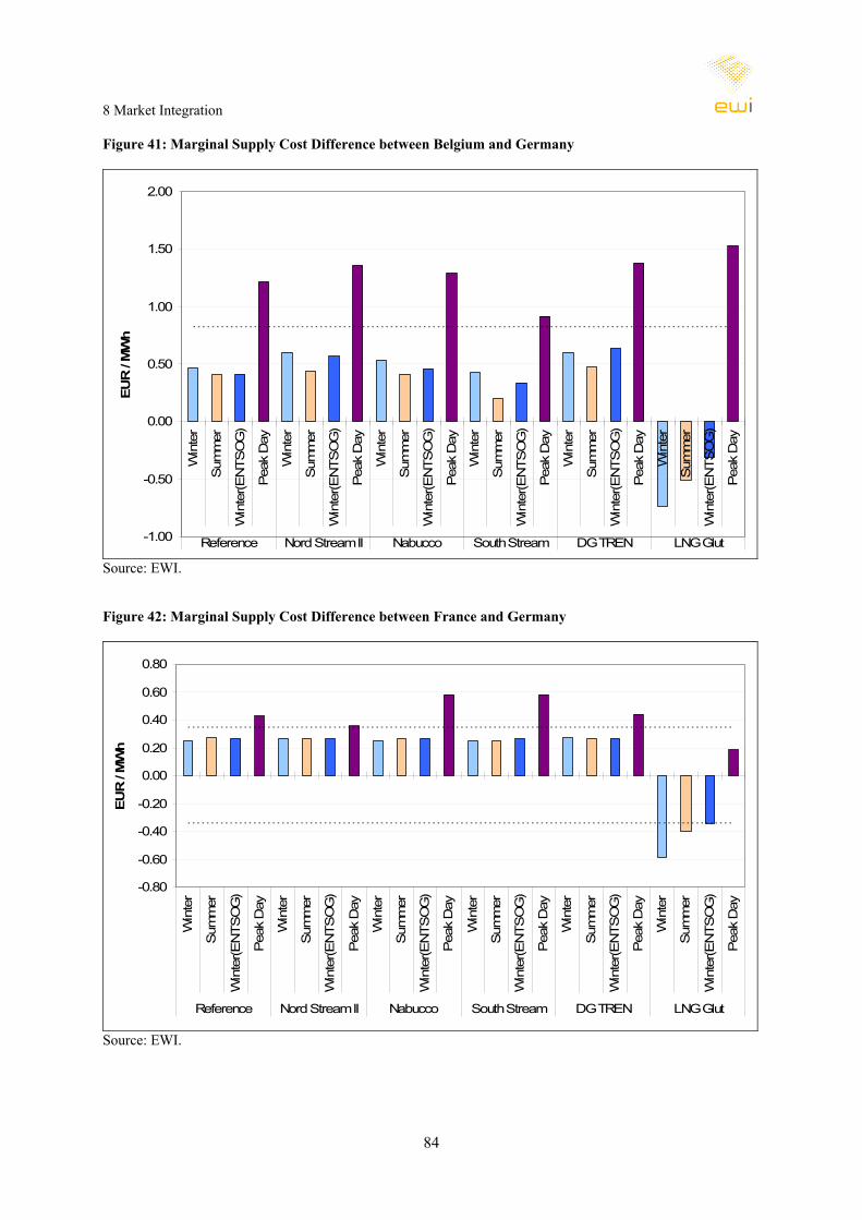
8 Market Integration
84
Figure 41: Marginal Supply Cost Difference between Belgium and Germany
-1.00
-0.50
0.00
0.50
1.00
1.50
2.00W
inte
r
Sum
mer
Win
ter(E
NTS
OG
)
Pea
k D
ay
Win
ter
Sum
mer
Win
ter(E
NTS
OG
)
Pea
k D
ay
Win
ter
Sum
mer
Win
ter(E
NTS
OG
)
Pea
k D
ay
Win
ter
Sum
mer
Win
ter(E
NTS
OG
)
Pea
k D
ay
Win
ter
Sum
mer
Win
ter(E
NTS
OG
)
Pea
k D
ay
Win
ter
Sum
mer
Win
ter(E
NTS
OG
)
Pea
k D
ay
Reference Nord Stream II Nabucco South Stream DG TREN LNG Glut
EUR
/ M
Wh
Source: EWI.
Figure 42: Marginal Supply Cost Difference between France and Germany
-0.80
-0.60
-0.40
-0.20
0.00
0.20
0.40
0.60
0.80
Win
ter
Sum
mer
Win
ter(E
NTS
OG
)
Pea
k D
ay
Win
ter
Sum
mer
Win
ter(E
NTS
OG
)
Pea
k D
ay
Win
ter
Sum
mer
Win
ter(E
NTS
OG
)
Pea
k D
ay
Win
ter
Sum
mer
Win
ter(E
NTS
OG
)
Pea
k D
ay
Win
ter
Sum
mer
Win
ter(E
NTS
OG
)
Pea
k D
ay
Win
ter
Sum
mer
Win
ter(E
NTS
OG
)
Pea
k D
ay
Reference Nord Stream II Nabucco South Stream DG TREN LNG Glut
EUR
/ M
Wh
Source: EWI.
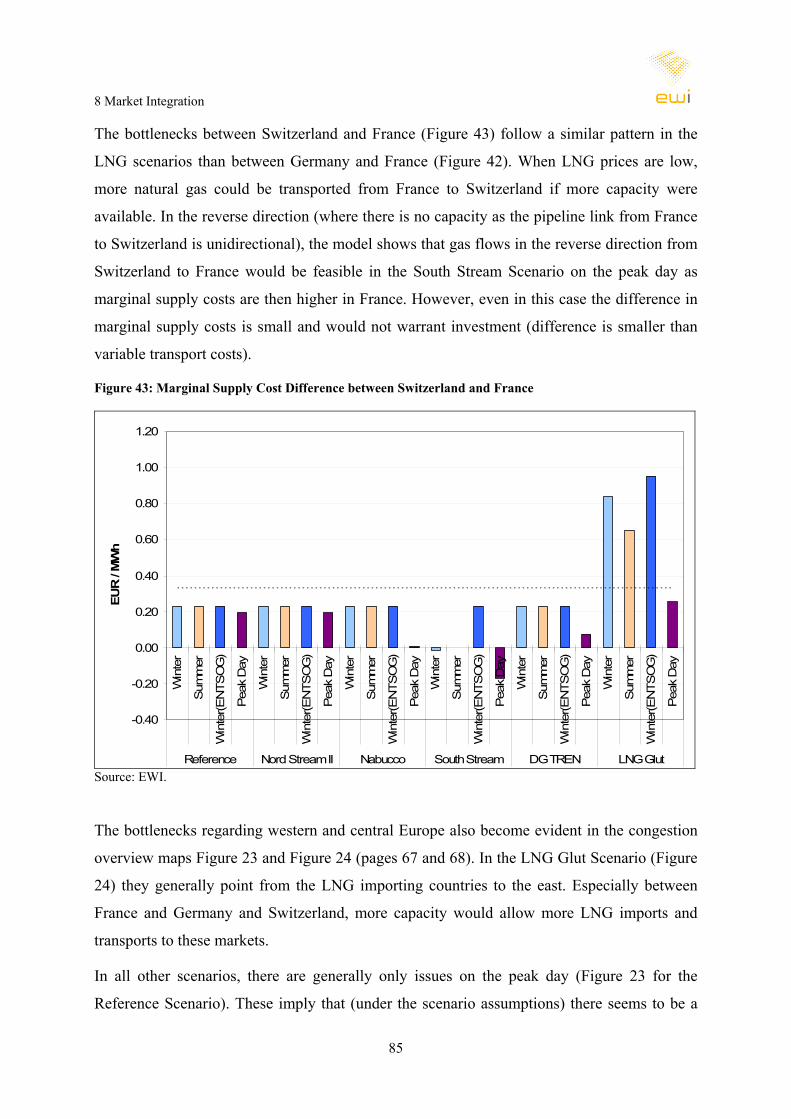
8 Market Integration
85
The bottlenecks between Switzerland and France (Figure 43) follow a similar pattern in the
LNG scenarios than between Germany and France (Figure 42). When LNG prices are low,
more natural gas could be transported from France to Switzerland if more capacity were
available. In the reverse direction (where there is no capacity as the pipeline link from France
to Switzerland is unidirectional), the model shows that gas flows in the reverse direction from
Switzerland to France would be feasible in the South Stream Scenario on the peak day as
marginal supply costs are then higher in France. However, even in this case the difference in
marginal supply costs is small and would not warrant investment (difference is smaller than
variable transport costs).
Figure 43: Marginal Supply Cost Difference between Switzerland and France
-0.40
-0.20
0.00
0.20
0.40
0.60
0.80
1.00
1.20
Win
ter
Sum
mer
Win
ter(E
NTS
OG
)
Pea
k D
ay
Win
ter
Sum
mer
Win
ter(E
NTS
OG
)
Pea
k D
ay
Win
ter
Sum
mer
Win
ter(E
NTS
OG
)
Pea
k D
ay
Win
ter
Sum
mer
Win
ter(E
NTS
OG
)
Pea
k D
ay
Win
ter
Sum
mer
Win
ter(E
NTS
OG
)
Pea
k D
ay
Win
ter
Sum
mer
Win
ter(E
NTS
OG
)
Pea
k D
ay
Reference Nord Stream II Nabucco South Stream DG TREN LNG Glut
EUR
/ M
Wh
Source: EWI.
The bottlenecks regarding western and central Europe also become evident in the congestion
overview maps Figure 23 and Figure 24 (pages 67 and 68). In the LNG Glut Scenario (Figure
24) they generally point from the LNG importing countries to the east. Especially between
France and Germany and Switzerland, more capacity would allow more LNG imports and
transports to these markets.
In all other scenarios, there are generally only issues on the peak day (Figure 23 for the
Reference Scenario). These imply that (under the scenario assumptions) there seems to be a

8 Market Integration
86
relative shortage of natural gas in Belgium, the Netherlands and France on the peak day
indicating demand for additional import capacity from all neighbouring countries (except
Spain). Reflecting on the assumptions confirms this: with respect to storages – which provide
significant swing supply in times of exceptionally high demand –, capacity additions in the
aforementioned countries are rather low compared to, for example, Germany, the UK or Italy
(see Figure 7 in Section 4.3). Furthermore, the detailed storage data (Appendix Table 12)
reveals that a large share of these additional storage capacities, especially in the Netherlands,
comes from depleted gas fields converted into underground gas storages (e.g. Bergermeer
storage). While depleted gas fields can generally store large volumes of gas, their withdrawal
rates are limited. Hence, these storages are not able to release large volumes of gas in a short
time period as required on a peak demand day. This effect is further amplified by the relative
magnitude of the peak day in Belgium, France, the Netherlands and Luxembourg (which is
supplied largely via Belgium): Figure 5 on page 32 shows that these four countries are
amongst the six countries where the peak day demand exceeds 250 percent of average daily
demand. (Only Denmark and Romania have similarly high relative peak day demands.)
These circumstances lead to relatively higher costs of providing the marginal (price setting)
gas volumes to consumers in this group of countries (compared to their neighbours). Never-
theless, as stated previously, the resulting congestion is only relevant temporary (on a concur-
rent peak day).
8.8 Iberian Peninsula and France
Again, with the assumed expansion of capacities between Spain and Portugal and Spain and
France, physical market integration between these countries is well developed according to
the model simulations in all scenarios.
Between Portugal and Spain, no bottlenecks can be identified (see Figure 44).
A differentiated consideration is required for the interconnection of the Spanish and French
gas markets.
As described in Section 4.3, the South Stream Scenario does not contain the MidCat pipeline
between Spain and France. Hence, capacity between the countries is smaller than in the other
scenarios. However, the results show that in this scenario, the simulations do not find a
significant differential in marginal supply costs between Spain and France (see Figure 45).
These findings presume that the global LNG market is working efficiently in the sense that
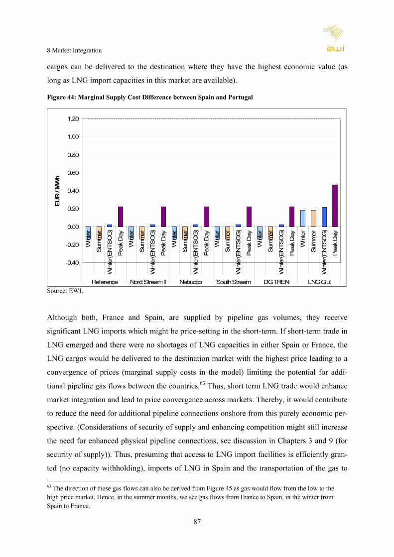
8 Market Integration
87
cargos can be delivered to the destination where they have the highest economic value (as
long as LNG import capacities in this market are available).
Figure 44: Marginal Supply Cost Difference between Spain and Portugal
-0.40
-0.20
0.00
0.20
0.40
0.60
0.80
1.00
1.20
Win
ter
Sum
mer
Win
ter(E
NTS
OG
)
Pea
k D
ay
Win
ter
Sum
mer
Win
ter(E
NTS
OG
)
Pea
k D
ay
Win
ter
Sum
mer
Win
ter(E
NTS
OG
)
Pea
k D
ay
Win
ter
Sum
mer
Win
ter(E
NTS
OG
)
Pea
k D
ay
Win
ter
Sum
mer
Win
ter(E
NTS
OG
)
Pea
k D
ay
Win
ter
Sum
mer
Win
ter(E
NTS
OG
)
Pea
k D
ay
Reference Nord Stream II Nabucco South Stream DG TREN LNG Glut
EUR
/ M
Wh
Source: EWI.
Although both, France and Spain, are supplied by pipeline gas volumes, they receive
significant LNG imports which might be price-setting in the short-term. If short-term trade in
LNG emerged and there were no shortages of LNG capacities in either Spain or France, the
LNG cargos would be delivered to the destination market with the highest price leading to a
convergence of prices (marginal supply costs in the model) limiting the potential for addi-
tional pipeline gas flows between the countries.63 Thus, short term LNG trade would enhance
market integration and lead to price convergence across markets. Thereby, it would contribute
to reduce the need for additional pipeline connections onshore from this purely economic per-
spective. (Considerations of security of supply and enhancing competition might still increase
the need for enhanced physical pipeline connections, see discussion in Chapters 3 and 9 (for
security of supply)). Thus, presuming that access to LNG import facilities is efficiently gran-
ted (no capacity withholding), imports of LNG in Spain and the transportation of the gas to 63 The direction of these gas flows can also be derived from Figure 45 as gas would flow from the low to the high price market. Hence, in the summer months, we see gas flows from France to Spain, in the winter from Spain to France.

8 Market Integration
88
France would not be economic unless all French LNG terminals are fully utilised. Neverthe-
less, on the peak demand day in the case of the LNG Glut Scenario, even with MidCat, higher
gas flows from Spain to France would be economically viable as the price difference between
these countries exceeds the transport costs in this case, as the LNG import capacity limit in
France is reached.
Figure 45: Marginal Supply Cost Difference between France and Spain
-1.00
-0.50
0.00
0.50
1.00
1.50
2.00
Win
ter
Sum
mer
Win
ter(E
NTS
OG
)
Pea
k D
ay
Win
ter
Sum
mer
Win
ter(E
NTS
OG
)
Pea
k D
ay
Win
ter
Sum
mer
Win
ter(E
NTS
OG
)
Pea
k D
ay
Win
ter
Sum
mer
Win
ter(E
NTS
OG
)
Pea
k D
ay
Win
ter
Sum
mer
Win
ter(E
NTS
OG
)
Pea
k D
ay
Win
ter
Sum
mer
Win
ter(E
NTS
OG
)
Pea
k D
ay
Reference Nord Stream II Nabucco South Stream DG TREN LNG Glut
EUR
/ M
Wh
Source: EWI.
8.9 South-South East: Romania, Bulgaria, Greece and Turkey
For the EU member states in south-eastern Europe, the model simulations also yield relatively
high market integration – with the exception of Greece on the peak days in the non-Nabucco
scenarios.64 As the peak day sensitivity simulated concurrent peak days in all countries
covered in the study, this also applies to Turkey which transits gas to Greece via the existing
(and assumed to be expanded) pipeline links. However, our model simulations show that
Turkey, which witnesses generally high demand growth, may not be able to transit large
volumes of natural gas on days of high domestic demand. Hence, such high demand in Turkey
can lead to a reduction of the gas flows from Turkey to Greece resulting in shortages in
64 I.e. scenarios Reference, Nord Stream II and South Stream.
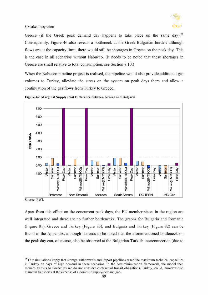
8 Market Integration
89
Greece (if the Greek peak demand day happens to take place on the same day).65
Consequently, Figure 46 also reveals a bottleneck at the Greek-Bulgarian border: although
flows are at the capacity limit, there would still be shortages in Greece on the peak day. This
is the case in all scenarios without Nabucco. (It needs to be noted that these shortages in
Greece are small relative to total consumption, see Section 8.10.)
When the Nabucco pipeline project is realised, the pipeline would also provide additional gas
volumes to Turkey, alleviate the stress on the system on peak days there and allow a
continuation of the gas flows from Turkey to Greece.
Figure 46: Marginal Supply Cost Difference between Greece and Bulgaria
-1.00
0.00
1.00
2.00
3.00
4.00
5.00
6.00
7.00
Win
ter
Sum
mer
Win
ter(E
NTS
OG
)
Pea
k D
ay
Win
ter
Sum
mer
Win
ter(E
NTS
OG
)
Pea
k D
ay
Win
ter
Sum
mer
Win
ter(E
NTS
OG
)
Pea
k D
ay
Win
ter
Sum
mer
Win
ter(E
NTS
OG
)
Pea
k D
ay
Win
ter
Sum
mer
Win
ter(E
NTS
OG
)
Pea
k D
ay
Win
ter
Sum
mer
Win
ter(E
NTS
OG
)
Pea
k D
ay
Reference Nord Stream II Nabucco South Stream DG TREN LNG Glut
EUR
/ M
Wh
Source: EWI.
Apart from this effect on the concurrent peak days, the EU member states in the region are
well integrated and there are no further bottlenecks. The graphs for Bulgaria and Romania
(Figure 81), Greece and Turkey (Figure 83), and Bulgaria and Turkey (Figure 82) can be
found in the Appendix, although it needs to be noted that the aforementioned bottleneck on
the peak day can, of course, also be observed at the Bulgarian-Turkish interconnection (due to
65 Our simulations imply that storage withdrawals and import pipelines reach the maximum technical capacities in Turkey on days of high demand in these scenarios. In the cost-minimization framework, the model then reduces transits to Greece as we do not consider contractual transit obligations. Turkey, could, however also maintain transports at the expense of a domestic supply-demand gap.
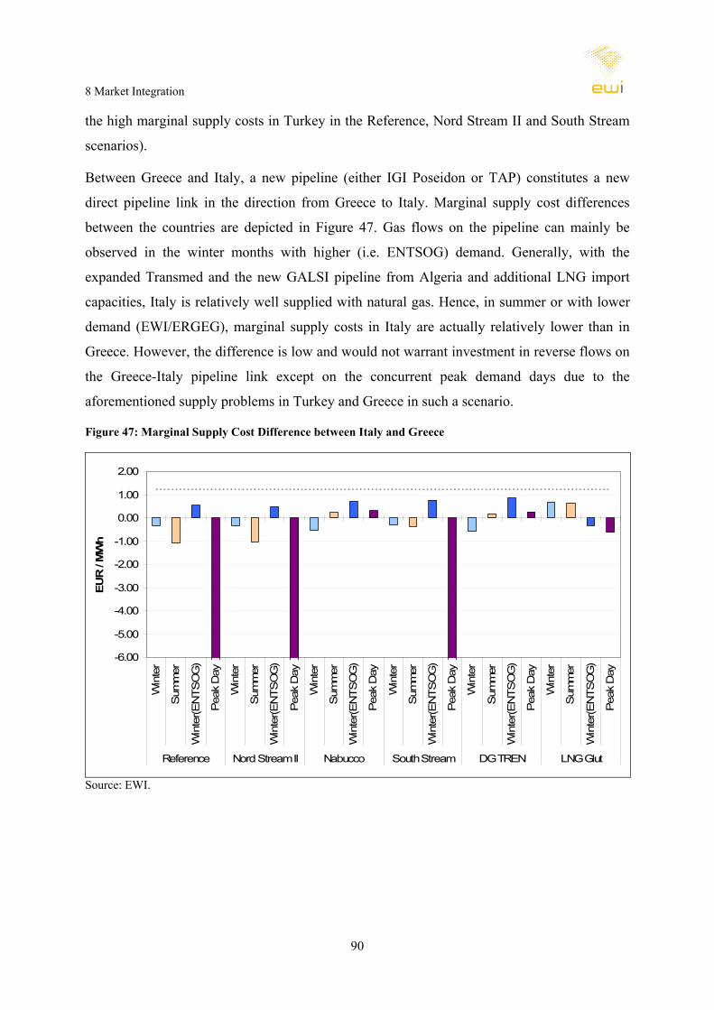
8 Market Integration
90
the high marginal supply costs in Turkey in the Reference, Nord Stream II and South Stream
scenarios).
Between Greece and Italy, a new pipeline (either IGI Poseidon or TAP) constitutes a new
direct pipeline link in the direction from Greece to Italy. Marginal supply cost differences
between the countries are depicted in Figure 47. Gas flows on the pipeline can mainly be
observed in the winter months with higher (i.e. ENTSOG) demand. Generally, with the
expanded Transmed and the new GALSI pipeline from Algeria and additional LNG import
capacities, Italy is relatively well supplied with natural gas. Hence, in summer or with lower
demand (EWI/ERGEG), marginal supply costs in Italy are actually relatively lower than in
Greece. However, the difference is low and would not warrant investment in reverse flows on
the Greece-Italy pipeline link except on the concurrent peak demand days due to the
aforementioned supply problems in Turkey and Greece in such a scenario.
Figure 47: Marginal Supply Cost Difference between Italy and Greece
-6.00
-5.00
-4.00
-3.00
-2.00
-1.00
0.00
1.00
2.00
Win
ter
Sum
mer
Win
ter(E
NTS
OG
)
Pea
k D
ay
Win
ter
Sum
mer
Win
ter(E
NTS
OG
)
Pea
k D
ay
Win
ter
Sum
mer
Win
ter(E
NTS
OG
)
Pea
k D
ay
Win
ter
Sum
mer
Win
ter(E
NTS
OG
)
Pea
k D
ay
Win
ter
Sum
mer
Win
ter(E
NTS
OG
)
Pea
k D
ay
Win
ter
Sum
mer
Win
ter(E
NTS
OG
)
Pea
k D
ay
Reference Nord Stream II Nabucco South Stream DG TREN LNG Glut
EUR
/ M
Wh
Source: EWI.
8 Market Integration
91
8.10 Security of Supply Implications of the Identified Bottlenecks
The preceding sections identified a number of bottlenecks leading to marginal supply cost
differences between countries and, hence, temporarily or permanently non-integrated markets.
However, some of the bottlenecks also have more significant implications in the sense that the
deliverability of natural gas in some countries is compromised severely. Hence, in some cases
the assumed import capacities plus domestic output plus possible storage withdrawals are not
sufficient to meet domestic demand on the peak day or on winter days in general leading to
supply-demand gaps.
Figure 48 summarises the scope of these disruptions in all affected countries for all relevant
scenarios66 on an average winter day with ENTSOG demand and for the peak demand day as
a percentage of the respective total consumption on that day. Four EU member states are
affected. As discussed in Section 8.5, a permanent significant bottleneck between Denmark
and Germany compromises the supply situation in Sweden and Denmark. Denmark is,
thereby, only affected on the peak demand day. Due to the shortage of gas in the country,
exports to Sweden, however, fully cease in winter. Demand disruptions in Hungary are
smaller, only around 15 percent of consumption, and only in the scenarios without a new
major import pipeline project in south-eastern Europe. The peak day issues regarding Greece
are discussed in Section 8.9. Figure 48 illustrates, however, that the scope of the demand
disruption on the concurrent peak day only amounts to around five percent of peak day
consumption.
Apart from these EU member states, the three Balkan countries with a gas industry also suffer
under insufficient import capacities given the assumed pipeline expansions and demand
developments. This is especially severe in Bosnia and Herzegovina when there are shortages
in Hungary as the country solely depends on gas imports via Hungary (Serbia at least has a
storage facility). In the other scenarios, and the other two countries (Serbia and Macedonia),
the supply shortages never exceed 30 percent of daily consumption. (It needs to be noted that
gas demand projections for this region are associated with a very high degree of uncertainty.
Furthermore, not all realistic pipeline expansion may be published clearly.67 Hence, the model
66 The LNG Glut Scenario is not considered in this section and in Chapter 9 (Security of Supply) as it is based on the same infrastructure assumptions as the DG TREN scenario and therefore does not yield any additional insights on security of supply or possible supply demand gaps. 67 Apart from taking into account the ENTSOG (2009) assumptions (which yield similar results the respect to demand-capacity gaps in those countries), infrastructure data was also compared with publications of the Energy
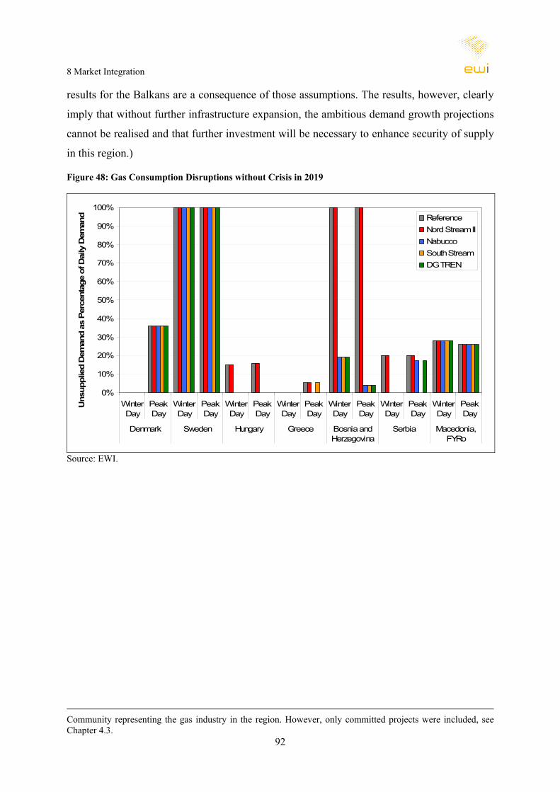
8 Market Integration
92
results for the Balkans are a consequence of those assumptions. The results, however, clearly
imply that without further infrastructure expansion, the ambitious demand growth projections
cannot be realised and that further investment will be necessary to enhance security of supply
in this region.)
Figure 48: Gas Consumption Disruptions without Crisis in 2019
0%
10%
20%
30%
40%
50%
60%
70%
80%
90%
100%
WinterDay
PeakDay
WinterDay
PeakDay
WinterDay
PeakDay
WinterDay
PeakDay
WinterDay
PeakDay
WinterDay
PeakDay
WinterDay
PeakDay
Denmark Sweden Hungary Greece Bosnia andHerzegovina
Serbia Macedonia,FYRo
Uns
uppl
ied
Dem
and
as P
erce
ntag
e of
Dai
ly D
eman
d
ReferenceNord Stream IINabuccoSouth StreamDG TREN
Source: EWI.
Community representing the gas industry in the region. However, only committed projects were included, see Chapter 4.3.
9 Security of Supply Simulations
93
9 Security of Supply Simulations This chapter presents the results of the security of supply sensitivities. Both stress scenarios
are discussed separately in the following two sections with respect to the consequences for
consumers (demand reduction and price effects) and the simulated optimal gas flow
diversions and additional storage withdrawals necessary to mitigate the consequences of the
stress scenarios. Section 9.3 analyses the impacts of the two stress scenarios on market
integration and specifically on the bottlenecks identified in Chapter 8.
Generally, it has to be noted that the model simulations take the demand assumptions as given
and compute how demand is met during such a crisis – or what share of demand cannot be
met. Hence, the results abstract from all possible demand side measures to mitigate supply
disruptions. Furthermore, it needs to be stressed that the model simulations are non-technical.
I.e. pipeline operations including pressures are not simulated. Hence, it is not possible to
compute supply disruptions which might be caused by pressure declines as a consequence of
stopped gas flows at one import point into a TSO network. Instead, it is assumed that if the
gas volumes can be replaced from other sources in such a case, the underlying technical
components of the system ensure that the pipeline network can continue to operate and supply
gas. This approach might, thereby, miss to highlight some supply disruptions caused by
technical issues in pipeline grids.
However, previous analysis with the applied model, for instance of the 2009 Russia-Ukraine
crisis, have shown that model is able to match actual supply disruptions in case of a crisis
situation quite well (see Bettzüge and Lochner (2009) and Bettzüge (2009)).
9.1 Four Week Disruption of Ukraine Transits in 2019
This stress scenario assumes that all transits of natural gas via Ukraine are halted for a
duration of 28 days.68 This period includes the peak demand day.69 This security of supply
simulation, hence, assumes a repetition of the January 2009 Russian-Ukrainian gas conflict
with a prolongation to four weeks (instead of 13 days). In our model simulations, transits via
Ukraine in January 2019 are between 186 to 345 million cubic metres per day (South Stream
and Reference Scenario respectively) depending on which alternative infrastructure projects
for Russian gas exports to Europe are available (Nord Stream II, South Stream). Hence, the
68 I.e. for four weeks starting the first Friday in January. 69 Assumed to be on the fourth Wednesday in January.
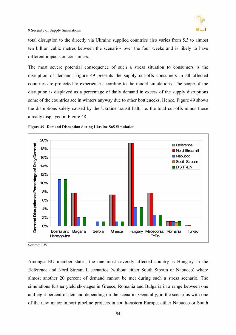
9 Security of Supply Simulations
94
total disruption to the directly via Ukraine supplied countries also varies from 5.3 to almost
ten billion cubic metres between the scenarios over the four weeks and is likely to have
different impacts on consumers.
The most severe potential consequence of such a stress situation to consumers is the
disruption of demand. Figure 49 presents the supply cut-offs consumers in all affected
countries are projected to experience according to the model simulations. The scope of the
disruption is displayed as a percentage of daily demand in excess of the supply disruptions
some of the countries see in winters anyway due to other bottlenecks. Hence, Figure 49 shows
the disruptions solely caused by the Ukraine transit halt, i.e. the total cut-offs minus those
already displayed in Figure 48.
Figure 49: Demand Disruption during Ukraine SoS Simulation
0%
2%
4%
6%
8%
10%
12%
14%
16%
18%
20%
Bosnia andHerzegovina
Bulgaria Serbia Greece Hungary Macedonia,FYRo
Romania TurkeyDem
and
Dis
rupt
ion
as P
erce
ntag
e of
Dai
ly D
eman
d
ReferenceNord Stream IINabuccoSouth StreamDG TREN
Source: EWI.
Amongst EU member states, the one most severely affected country is Hungary in the
Reference and Nord Stream II scenarios (without either South Stream or Nabucco) where
almost another 20 percent of demand cannot be met during such a stress scenario. The
simulations further yield shortages in Greece, Romania and Bulgaria in a range between one
and eight percent of demand depending on the scenario. Generally, in the scenarios with one
of the new major import pipeline projects in south-eastern Europe, either Nabucco or South
9 Security of Supply Simulations
95
Stream, the consequences of the crisis to consumers are smaller (with South Stream even
more so than with Nabucco). The only country experiencing (albeit very minor) disruptions to
consumers in all scenarios is Romania. As this was not found to be the case in simulations of
shorter (two-week-) disruptions of Ukraine transits (not reported in this document), it can be
concluded that import, production and storage capacities of the country are sufficient for
coping with short, temporary disruptions of imports from Ukraine, but not with ones
stretching up to four weeks. For the Balkan countries with supply shortages without a crisis,
the demand disruptions are generally larger during a Ukraine transit halt.
Hence, apart from these countries, severe effects for consumers in the rest of Europe are not
projected by our simulations. Other consequences, however, could be price effects outside the
severely affected countries. As an indicator for these, Table 5 presents the maximum change
in marginal supply costs compared to a simulation without the disruption. It is important to
note that these are not projections of wholesale price changes which cannot be computed.
Market prices are impacted by other factors not taken into account by the model. Apart from
simplifications of the model (see Chapter 3), such as inelastic demand, these mainly relate to
uncertainty and expectations which are crucial for price formation in wholesale markets.
Hence, even in a fully functioning market, wholesale prices may deviate from marginal
supply costs. However, simulations of the January 2009 Russian-Ukrainian gas conflict with
the applied TIGER model yield marginal supply cost changes which are on average (except
the price spikes on the first day of the crisis) similar to those observed at the western and
central European gas trading points (Bettzüge and Lochner, 2009). Therefore, interpreting the
changes in short-run marginal supply costs of the simulations yields insights into the extra
costs to the gas industry caused by a disruption of Ukraine transits. The values in Table 5
represent the maximum changes in marginal supply costs for each scenario relative to an
otherwise identical time period without the crisis. (Due to the inelastic demand, marginal
supply costs cannot be computed in countries with disruptions to consumers as this causes
infinitely high marginal supply cost.)

9 Security of Supply Simulations
96
Table 5: Increases in Marginal Supply Costs in Ukraine SoS Simulation in 2019
Country Reference Nord Stream II Nabucco South Stream DG TRENAustria + 3.8 % + 3.7 % + 4.4 % + 2.7 % + 4.1 %Belgium + 1.1 % + 1.0 % + 0.4 % + 0.4 % + 0.8 %Bosnia and Herzegovina + 0.0 % + 0.0 % + 0.0 % + 0.0 % + 0.0 %Bulgaria + ∞ + ∞ + ∞ + 1.5 % + ∞Croatia + 0.2 % + 0.2 % + ∞ + 1.4 % + ∞Czech Republic + 2.1 % + 0.7 % + 2.3 % + 1.6 % + 0.8 %Denmark + 0.0 % + 0.0 % + 0.0 % + 0.0 % + 0.0 %Estonia - 7.2 % - 8.4 % - 7.5 % - 1.8 % - 8.4 %France (Northern Zone) + 0.4 % + 0.6 % + 0.1 % - 0.0 % + 0.4 %France (Southern Zone) + 0.0 % + 0.0 % - 0.0 % + 0.0 % + 0.0 %Germany (North) - 0.1 % - 0.2 % + 0.1 % + 0.4 % - 0.2 %Germany (South) + 1.1 % + 1.0 % + 1.5 % + 0.9 % + 1.2 %Great Britain (Bacton) - 0.1 % - 0.2 % - 0.1 % + 0.0 % - 0.2 %Great Britain (St. Fergus) - 0.1 % - 0.2 % - 0.1 % - 0.0 % - 0.2 %Greece + 0.4 % + 0.4 % + ∞ + 0.0 % + ∞Hungary + 0.0 % + 0.0 % + ∞ + 3.1 % + ∞Ireland - 0.1 % - 0.2 % - 0.1 % - 0.0 % - 0.1 %Italy (North) + 0.1 % + 0.1 % + 0.5 % + 0.1 % + 0.5 %Italy (South) + 0.1 % + 0.1 % + 0.1 % + 0.0 % + 0.3 %Latvia - 6.1 % - 6.4 % - 6.1 % - 1.4 % - 6.3 %Lithuania - 8.3 % - 7.8 % - 8.5 % - 1.7 % - 7.8 %Luxembourg + 1.1 % + 1.0 % + 0.4 % + 0.5 % + 0.8 %Macedonia + 0.0 % + 0.0 % + 0.0 % + 0.0 % + 0.0 %Netherlands + 1.1 % + 1.0 % + 0.4 % + 0.4 % + 0.8 %Norway - 0.0 % - 0.2 % - 0.2 % + 0.4 % + 0.0 %Poland - 0.0 % - 0.2 % + 0.3 % + 1.4 % - 0.3 %Portugal + 0.0 % + 0.0 % - 0.0 % - 0.0 % + 0.0 %Romania + ∞ + ∞ + ∞ + ∞ + ∞Serbia + 0.2 % + 0.2 % + 0.3 % + 1.5 % + 0.3 %Slovakia + 8.3 % + 6.4 % + 7.6 % + 5.3 % + 6.3 %Slovenia + 2.9 % + 2.9 % + 3.4 % + 1.4 % + 3.2 %Spain + 0.0 % + 0.0 % - 0.0 % - 0.0 % + 0.0 %Sweden + 0.0 % + 0.0 % + 0.0 % + 0.0 % + 0.0 %Switzerland + 0.3 % + 0.6 % + 0.5 % + 0.1 % + 0.5 %Turkey + 0.1 % + 0.1 % + ∞ + 0.0 % + ∞ Source: EWI.
For the countries where demand can be met during a crisis, the changes in marginal supply
costs are relatively small (also compared to simulations of the January 2009 crisis). The
largest rise is observed in the Slovak Republic as the country is normally solely dependent on
Russian imports via Ukraine and needs to be fully supplied from the west and its storages
during a potential supply disruption from the east. Noteworthy, increases in supply costs are
also observed for Austria, Slovenia and, to a smaller extent, the Czech Republic which also
continue to receive a large share of their gas imports via Ukraine in 2019 (see also the gas
flow analyses in Section 7.1). The countries which see supply disruptions in some scenarios
generally also experience a significant increase in marginal supply costs in the scenarios
where supply to consumers is maintained. Intuitively, the consequences for consumers in
eastern Europe with respect to cut-offs (Figure 49) and supply costs (Table 5) are the smallest

9 Security of Supply Simulations
97
in the South Stream Scenario as this project essentially constitutes an alternative route for
Russian gas to the countries otherwise depending on Ukraine transits.
In western Europe, the supply cost changes during such a crisis are found to be relatively
minor and do not exceed two percent relative to a simulation without a disruption. (In some
countries, which are supplied by Russian gas via other routes, marginal supply costs actually
slightly decline. This is due to the fact that Russian gas volumes partially have to be rerouted
when transit via Ukraine is not possible causing a higher availability of Russian gas volumes
in other regions. In the simulated competitive market, more supply leads ceteris paribus to
lower marginal costs (or prices).)
A map of the supply cost changes for the Reference case (together with new bottlenecks
during the crisis) can be found in Section 9.3 (Figure 52). (For the other scenarios, the maps
can be found in the Appendix starting on page 141.)
How the disruptions are compensated in the model simulations is illustrated in Figure 50,
which displays the difference in average gas imports, gas production, storage withdrawals,
and consumer cut-offs in the respective time period between the simulation with and without
Ukraine crisis. It is thereby clear that natural gas storages compensate most of the transit
disruption. Production flexibility in January is not high as most EU production facilities
already operate near the maximum in a normal winter. Rerouting of Russian gas to the EU is
also only possible in the scenarios with either Nord Stream II or South Stream as all Russian
export pipelines would already be fully utilised in winter without either of those projects.
Additional storage withdrawals are not only observed in the countries directly affected by the
crisis but, almost to a similar extent volume-wise, also in Italy and Germany to enable west-
to-east gas flows. Additional LNG imports (included in Imports/Production in Figure 50) are
minor as the majority of LNG import capacities are located in countries from where transport
to eastern Europe is not feasible (UK, France, Spain). Aggregated consumer cut-offs are, as
discussed previously, highest in the scenarios with no new pipeline project in south-eastern
Europe and lowest with South Stream. Generally, in the South Stream Scenario, transits via
Ukraine are significantly lower (see Chapter 7.1). Hence, less compensation is necessary in
case of a transit disruption leading to relatively lower additional withdrawals from storages in
all countries.
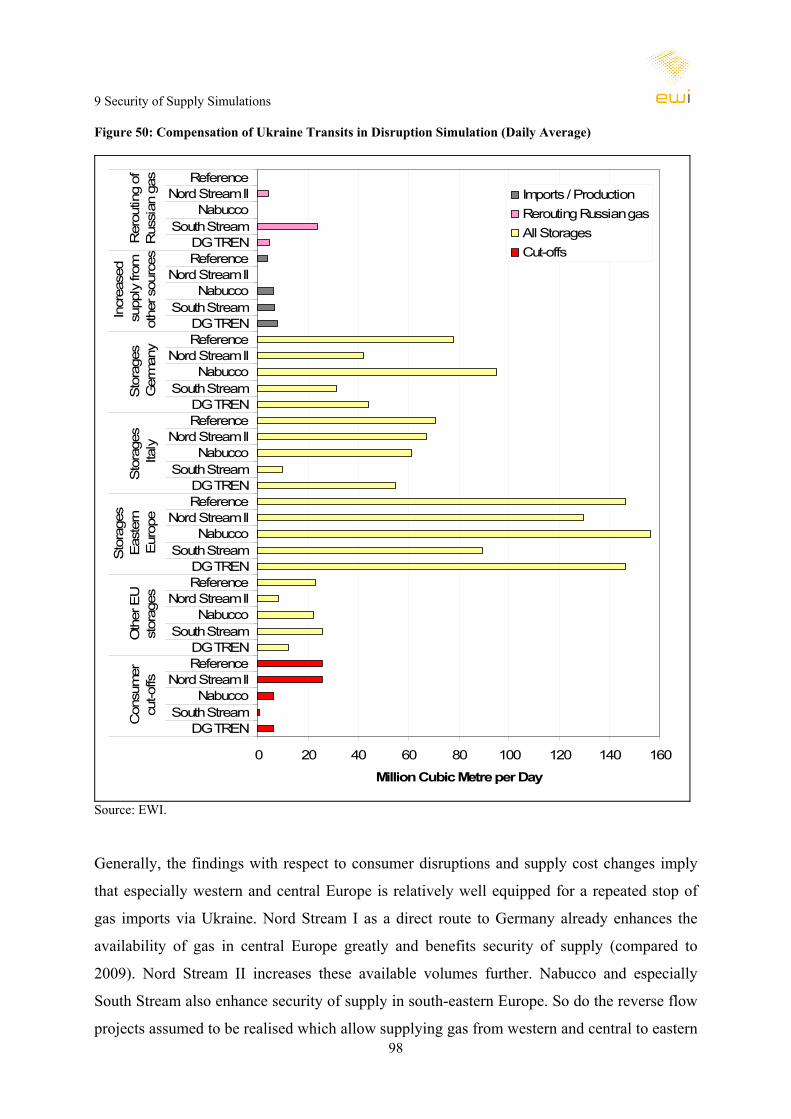
9 Security of Supply Simulations
98
Figure 50: Compensation of Ukraine Transits in Disruption Simulation (Daily Average)
0 20 40 60 80 100 120 140 160
DG TRENSouth Stream
NabuccoNord Stream II
ReferenceDG TREN
South StreamNabucco
Nord Stream IIReferenceDG TREN
South StreamNabucco
Nord Stream IIReferenceDG TREN
South StreamNabucco
Nord Stream IIReferenceDG TREN
South StreamNabucco
Nord Stream IIReferenceDG TREN
South StreamNabucco
Nord Stream IIReferenceDG TREN
South StreamNabucco
Nord Stream IIReference
Con
sum
ercu
t-offs
Oth
er E
Ust
orag
es
Sto
rage
sE
aste
rnE
urop
eS
tora
ges
Italy
Sto
rage
sG
erm
any
Incr
ease
dsu
pply
from
othe
r sou
rces
Rer
outin
g of
Rus
sian
gas
Million Cubic Metre per Day
Imports / ProductionRerouting Russian gasAll StoragesCut-offs
Source: EWI.
Generally, the findings with respect to consumer disruptions and supply cost changes imply
that especially western and central Europe is relatively well equipped for a repeated stop of
gas imports via Ukraine. Nord Stream I as a direct route to Germany already enhances the
availability of gas in central Europe greatly and benefits security of supply (compared to
2009). Nord Stream II increases these available volumes further. Nabucco and especially
South Stream also enhance security of supply in south-eastern Europe. So do the reverse flow
projects assumed to be realised which allow supplying gas from western and central to eastern
9 Security of Supply Simulations
99
Europe during a disruption of Ukraine imports. Storages have the most important role in
maintaining supply to consumers. Together, additional storage withdrawals in central (Italy,
Germany) and eastern Europe contribute more than 90 percent to compensating the
interrupted transits via Ukraine. Nevertheless, full security of supply (i.e. the avoidance of
supply cut-offs to consumers) towards the simulated stress test is not achieved in any of the
scenarios. Especially when there are no new major infrastructure projects in south-eastern
Europe, supply disruptions cannot be avoided. We find that bottlenecks also still exist in the
west-to-east direction, for instance from Germany to the Czech Republic or from the Czech to
the Slovak Republic, which prevents further gas flows from central and western to eastern
Europe. (For a full discussion of identified congestion in the crisis simulations, see Section
9.3.) Apart from the Balkans, the most severely affected EU member states are Hungary,
Bulgaria and Greece with supply shortfalls between seven and 20 percent of demand.
Furthermore, for the mitigation scenarios described here to materialise, the establishment of
an efficiently working and competitive gas market (which sends the required price signals for
flow diversions and storage withdrawals) is required. If it is not in place in such a crisis, or if,
for instance, government intervention prevents cross-border solidarity (which is efficient from
a total system perspective), supply disruptions to consumers or price effects may be larger.
(See also discussion on the assumptions of the model (Chapter 3) or at the end of the next
section.)
9.2 Four Week Disruption of Algerian Exports in 2019
Like the Ukraine transit disruption, this stress scenario assumes that all exports of natural gas
from Algeria via pipeline are halted for a duration of 28 days.70 This period includes the peak
demand day.71 Regarding global LNG supplies – which are also likely to be affected from an
Algerian gas export stop –, it is assumed that 25 percent of all LNG cargos to Europe in this
time period do not arrive. This figure is based on the fact that Algerian LNG supplies to
Europe made up 35 percent in 2008 (BP, 2009). Taking into account that many new LNG
liquefaction projects are going online around the world in the period from 2009 to 2014, this
relative share is likely to decline (not implying that absolute Algerian LNG exports to Europe
fall). With respect to all other European LNG cargos, it is assumed that these can be rerouted
between European countries, i.e. that supplies to Spain can be increased by decreasing
70 I.e. for four weeks starting the first Friday in January. 71 Assumed to be on the fourth Wednesday in January.
9 Security of Supply Simulations
100
supplies to the UK. However, this rerouting only becomes effective after the first week of the
crisis as it may take some time. Hence, 25 percent less LNG to Europe would be a reasonable
estimate if Algeria fully ceased to export LNG72 (and pipeline gas). The resulting total
disruptions of pipeline and LNG supplies range between 320 and 343 million cubic meters per
day depending on the scenario and is, hence, similar in scope to the Ukraine security of
supply sensitivity (Section 9.1).
Within the modelling constraint that potential supply disruptions caused by technical system
issues as a consequence of the drop-out of one (Italy) or two (Spain) system entry points are
not detected, the model only finds limited supply disruptions as a consequence of the Algerian
export stop. Gas flow diversions, the rerouting of LNG cargos, additional withdrawals from
storages, and slight production increases by other suppliers are found to be able to mitigate
the consequences of the hypothetical Algerian export stop from a capacity perspective.
The individual contributions of these compensation measures are quantified in Figure 51. Like
in the Ukraine stress scenario, the most additional supply comes from gas storages. Additional
withdrawals from storages in the two most directly affected countries, Spain and Italy,
compensate about 40 percent of the total deficit together. The largest share, however, comes
from underground gas storages in Italy which can provide about 100 million cubic metres of
gas additionally. In Spain, however, there is much less storage capacity so additional
withdrawals can only amount to about 40 million cubic metres a day. The decline in total
LNG supplies to Europe also affects other countries including Great Britain (average daily
decline in LNG imports of 60 million cubic metres per day), the Netherlands (up to -54),
France (up to -27), and Portugal (-7). Spanish and Italian LNG imports decline by about 18
and 8 million cubic metres per day on average (see Table 14 in the Appendix for the decline
of LNG cargos to all LNG importing countries and all scenarios). Consequently, other gas
volumes in various European countries need to be procured from different sources to
compensate for the LNG import shortfalls. About 18 percent of these volumes come from
British gas storages, the majority of the remaining volumes from storages in other countries,
most notable UGS in France and Germany. Again, as discussed in the context of the Ukraine
security of supply simulation in Section 9.1, the flexibility of European production to increase
output further in the winter months is limited. Hence, increases in production in the EU and
imports from non-EU countries cannot significantly help to mitigate the effects of a 72 Some of the Algerian LNG cargos may also be replaced by LNG from other sources as a consequence of the price effect in Europe.
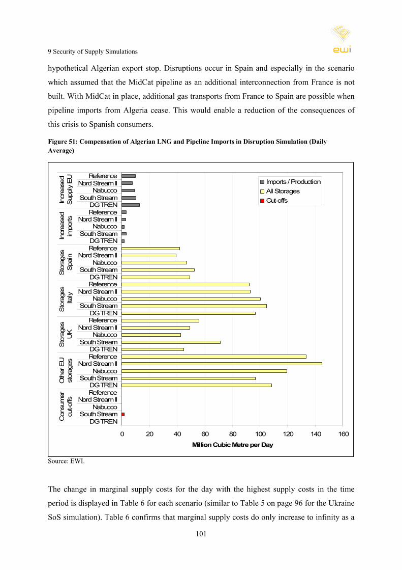
9 Security of Supply Simulations
101
hypothetical Algerian export stop. Disruptions occur in Spain and especially in the scenario
which assumed that the MidCat pipeline as an additional interconnection from France is not
built. With MidCat in place, additional gas transports from France to Spain are possible when
pipeline imports from Algeria cease. This would enable a reduction of the consequences of
this crisis to Spanish consumers.
Figure 51: Compensation of Algerian LNG and Pipeline Imports in Disruption Simulation (Daily Average)
0 20 40 60 80 100 120 140 160
DG TRENSouth Stream
NabuccoNord Stream II
ReferenceDG TREN
South StreamNabucco
Nord Stream IIReferenceDG TREN
South StreamNabucco
Nord Stream IIReferenceDG TREN
South StreamNabucco
Nord Stream IIReferenceDG TREN
South StreamNabucco
Nord Stream IIReferenceDG TREN
South StreamNabucco
Nord Stream IIReferenceDG TREN
South StreamNabucco
Nord Stream IIReference
Con
sum
ercu
t-offs
Oth
er E
Ust
orag
esS
tora
ges
UK
Sto
rage
s Ita
lyS
tora
ges
Spa
inIn
crea
sed
impo
rtsIn
crea
sed
Sup
ply
EU
Million Cubic Metre per Day
Imports / ProductionAll StoragesCut-offs
Source: EWI.
The change in marginal supply costs for the day with the highest supply costs in the time
period is displayed in Table 6 for each scenario (similar to Table 5 on page 96 for the Ukraine
SoS simulation). Table 6 confirms that marginal supply costs do only increase to infinity as a
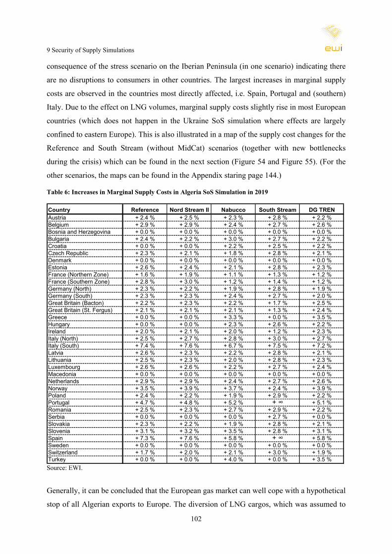
9 Security of Supply Simulations
102
consequence of the stress scenario on the Iberian Peninsula (in one scenario) indicating there
are no disruptions to consumers in other countries. The largest increases in marginal supply
costs are observed in the countries most directly affected, i.e. Spain, Portugal and (southern)
Italy. Due to the effect on LNG volumes, marginal supply costs slightly rise in most European
countries (which does not happen in the Ukraine SoS simulation where effects are largely
confined to eastern Europe). This is also illustrated in a map of the supply cost changes for the
Reference and South Stream (without MidCat) scenarios (together with new bottlenecks
during the crisis) which can be found in the next section (Figure 54 and Figure 55). (For the
other scenarios, the maps can be found in the Appendix staring page 144.)
Table 6: Increases in Marginal Supply Costs in Algeria SoS Simulation in 2019
Country Reference Nord Stream II Nabucco South Stream DG TRENAustria + 2.4 % + 2.5 % + 2.3 % + 2.8 % + 2.2 %Belgium + 2.9 % + 2.9 % + 2.4 % + 2.7 % + 2.6 %Bosnia and Herzegovina + 0.0 % + 0.0 % + 0.0 % + 0.0 % + 0.0 %Bulgaria + 2.4 % + 2.2 % + 3.0 % + 2.7 % + 2.2 %Croatia + 0.0 % + 0.0 % + 2.2 % + 2.5 % + 2.2 %Czech Republic + 2.3 % + 2.1 % + 1.8 % + 2.8 % + 2.1 %Denmark + 0.0 % + 0.0 % + 0.0 % + 0.0 % + 0.0 %Estonia + 2.6 % + 2.4 % + 2.1 % + 2.8 % + 2.3 %France (Northern Zone) + 1.6 % + 1.9 % + 1.1 % + 1.3 % + 1.2 %France (Southern Zone) + 2.8 % + 3.0 % + 1.2 % + 1.4 % + 1.2 %Germany (North) + 2.3 % + 2.2 % + 1.9 % + 2.8 % + 1.9 %Germany (South) + 2.3 % + 2.3 % + 2.4 % + 2.7 % + 2.0 %Great Britain (Bacton) + 2.2 % + 2.3 % + 2.2 % + 1.7 % + 2.5 %Great Britain (St. Fergus) + 2.1 % + 2.1 % + 2.1 % + 1.3 % + 2.4 %Greece + 0.0 % + 0.0 % + 3.3 % + 0.0 % + 3.5 %Hungary + 0.0 % + 0.0 % + 2.3 % + 2.6 % + 2.2 %Ireland + 2.0 % + 2.1 % + 2.0 % + 1.2 % + 2.3 %Italy (North) + 2.5 % + 2.7 % + 2.8 % + 3.0 % + 2.7 %Italy (South) + 7.4 % + 7.6 % + 6.7 % + 7.5 % + 7.2 %Latvia + 2.6 % + 2.3 % + 2.2 % + 2.8 % + 2.1 %Lithuania + 2.5 % + 2.3 % + 2.0 % + 2.8 % + 2.3 %Luxembourg + 2.6 % + 2.6 % + 2.2 % + 2.7 % + 2.4 %Macedonia + 0.0 % + 0.0 % + 0.0 % + 0.0 % + 0.0 %Netherlands + 2.9 % + 2.9 % + 2.4 % + 2.7 % + 2.6 %Norway + 3.5 % + 3.9 % + 3.7 % + 2.4 % + 3.9 %Poland + 2.4 % + 2.2 % + 1.9 % + 2.9 % + 2.2 %Portugal + 4.7 % + 4.8 % + 5.2 % + ∞ + 5.1 %Romania + 2.5 % + 2.3 % + 2.7 % + 2.9 % + 2.2 %Serbia + 0.0 % + 0.0 % + 0.0 % + 2.7 % + 0.0 %Slovakia + 2.3 % + 2.2 % + 1.9 % + 2.8 % + 2.1 %Slovenia + 3.1 % + 3.2 % + 3.5 % + 2.8 % + 3.1 %Spain + 7.3 % + 7.6 % + 5.8 % + ∞ + 5.8 %Sweden + 0.0 % + 0.0 % + 0.0 % + 0.0 % + 0.0 %Switzerland + 1.7 % + 2.0 % + 2.1 % + 3.0 % + 1.9 %Turkey + 0.0 % + 0.0 % + 4.0 % + 0.0 % + 3.5 % Source: EWI.
Generally, it can be concluded that the European gas market can well cope with a hypothetical
stop of all Algerian exports to Europe. The diversion of LNG cargos, which was assumed to

9 Security of Supply Simulations
103
be effective within Europe after a couple of days, allows to “spread” the consequences in the
form of increased marginal supply costs to a lot of consumers in many countries. However,
this also implies that mitigation of the disruption can take place in many countries: For
instance, storage volumes in the UK or Germany can help to compensate fewer LNG cargos
coming to north western European countries. These LNG cargos, in turn, can be diverted to
countries more exposed to Algerian (pipeline) gas such as Spain, Portugal and Italy.
Of course, apart from a competitive European gas market which provides the necessary price
signals for such diversions to occur, a largely competitive LNG market and sufficient LNG
import capacities in the different countries are required to realise the crisis mitigation scenario
outlined in this section. Apart from potential technical issues not covered by the model, a tight
LNG market, state intervention preventing supplies to other countries in a crisis, or other
inefficiencies might lead to further supply disruptions and larger price increases as described
here.
9.3 Implications on Market Integration
Chapter 8 outlined the findings of this study with respect to physical market integration in
Europe during summer and winter months (with different demand levels) and on a
hypothetical concurrent peak day in all European countries. As the previous two sections have
shown, SoS stress scenarios may imply changing relative supply cost structures and
diversions of gas flows. Both have an effect on the utilisation of infrastructure and, hence, the
evaluation of transport capacity and congestion. Therefore, this section summarises where
additional bottlenecks might occur if one of the two stress scenarios materialises.
Table 7 presents the bottlenecks computed by the model as a consequence of the supply
disruptions. Similar to Table 4 (page 65, location of bottlenecks without crisis), Table 7 lists
all investigated country pairs; bottlenecks between countries in a scenario are marked with
colours for the peak and/or average winter day respectively – uncoloured (white) fields mark
country pairs without additional congestion relative to the simulation without crisis. (The
colour thereby only indicates the type of day (peak vs. average winter) for better illustration.
Bottlenecks marked with R are in the reverse direction between the two countries relative to
the bottleneck identified at that location in times without crisis.) In addition to the table, the
directions of bottlenecks are displayed in Figure 52 and Figure 54 for the Ukraine and Algeria
SoS sensitivities of the Reference Scenario respectively.

9 Security of Supply Simulations
104
Generally, it can be noted that additional congestion largely occurs in the countries directly
affected by the supply disruptions and in regions where (other) bottlenecks are also evident
without a crisis (see Table 4). The latter is especially true for parts of eastern Europe where
additional congestions occurs in both SoS sensitivity simulations; albeit in the Ukrainian one
often in the reverse direction compared to the bottlenecks without crisis.
Table 7: Additional Bottlenecks as a Consequence of the Stress Simulations
Countries
Win
ter D
ay
(EN
TSO
G)
Peak
Dem
and
Day
Win
ter D
ay
(EN
TSO
G)
Peak
Dem
and
Day
Win
ter D
ay
(EN
TSO
G)
Peak
Dem
and
Day
Win
ter D
ay
(EN
TSO
G)
Peak
Dem
and
Day
Win
ter D
ay
(EN
TSO
G)
Peak
Dem
and
Day
Win
ter D
ay
(EN
TSO
G)
Peak
Dem
and
Day
Win
ter D
ay
(EN
TSO
G)
Peak
Dem
and
Day
Win
ter D
ay
(EN
TSO
G)
Peak
Dem
and
Day
Win
ter D
ay
(EN
TSO
G)
Peak
Dem
and
Day
Win
ter D
ay
(EN
TSO
G)
Peak
Dem
and
Day
ES and PTES and FRGB and IEGB and BEGB and NLBE and NLFR and BEDE and NLDE and BEDE and FRCH and DEFR and CHCH and ITDE and DKDE and PLCZ and DE-S*CZ and DE-E*AT and DEAT and IT R RAT and SIIT and SIHR and SIHR and HUAT and HUHU and ROAT and SKCZ and SK R R R R R RBG and ROBG and GRBG and TRGR and TRGR and IT*Czech border with south (Waidhaus) and east Germany (Olbernhau) respectivelyAdditional bottleneck on average winter day in Ukraine SoS simulation: and in Algeria SoS simulation:Additional bottleneck on peak demand day in Ukraine SoS simulation: and in Algeria SoS simulation:No additional bottleneck:Bottlenecks in reverse direction relative to simulations without SoS situation (previous chapter) are marked with R
Ukraine stress scenario Algeria stress scenario
DG TREN Refer-ence
Nord Stream II NabuccoRefer-
enceNord
Stream II Nabucco South Stream
South Stream DG TREN
Source: EWI.

9 Security of Supply Simulations
105
Additional Congestion in Ukraine SoS Simulation
Figure 52: Ukraine SoS Simulation (Reference): Additional Bottlenecks and Marginal Supply Costs Changes
R
R
R
R
Bottleneck in directionof arrow:
Average day
Peak day
(Grey colour impliesbottleneck also found in simulation withoutdisruption, see Chapter 8)
Source: EWI.
In the Ukraine SoS simulation (left hand side of Table 7), new bottlenecks are confined to
central and eastern Europe. Despite the reverse flow projects realised after the 2009 Russia-
Ukraine conflict, there are still some bottlenecks preventing additional west-to-east gas flows,
namely between eastern Germany and the Czech Republic (where Nord Stream volumes can
be routed south), the Czech and Slovak Republics and Austria and Hungary (although the
latter bottleneck also existed without a crisis in most of the scenarios). With respect to Greece
and Italy (which is investigated as a country pair because of the new offshore pipeline link
between the countries (although there is no capacity from Italy to Greece)), the results show
that a reverse flow on this pipeline would be beneficial in times of a disruption of Ukraine
transits. Bottlenecks in the Nord Stream II, Nabucco and DG TREN scenarios are similar to
the ones highlighted in Figure 52 (see Appendix C, page 141). In the South Stream Scenario,
however, the alternative Russian export route implies that gas volumes are routed through
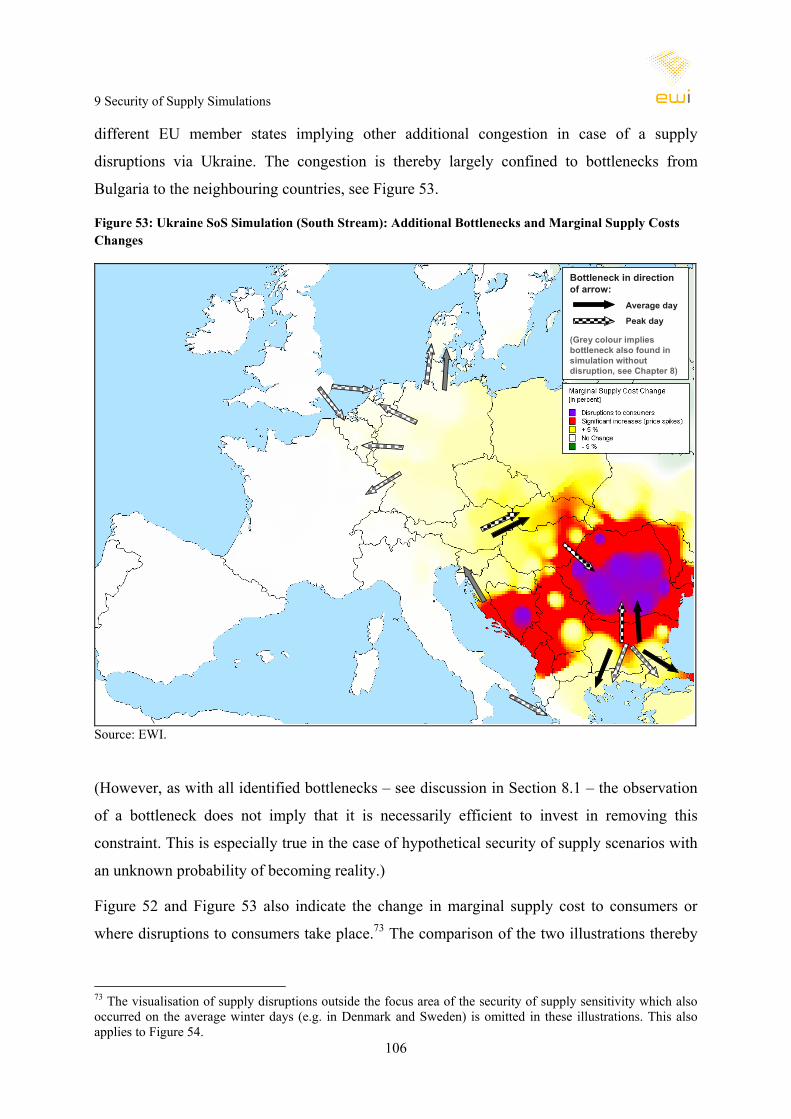
9 Security of Supply Simulations
106
different EU member states implying other additional congestion in case of a supply
disruptions via Ukraine. The congestion is thereby largely confined to bottlenecks from
Bulgaria to the neighbouring countries, see Figure 53.
Figure 53: Ukraine SoS Simulation (South Stream): Additional Bottlenecks and Marginal Supply Costs Changes
Bottleneck in directionof arrow:
Average day
Peak day
(Grey colour impliesbottleneck also found in simulation withoutdisruption, see Chapter 8)
Source: EWI.
(However, as with all identified bottlenecks – see discussion in Section 8.1 – the observation
of a bottleneck does not imply that it is necessarily efficient to invest in removing this
constraint. This is especially true in the case of hypothetical security of supply scenarios with
an unknown probability of becoming reality.)
Figure 52 and Figure 53 also indicate the change in marginal supply cost to consumers or
where disruptions to consumers take place.73 The comparison of the two illustrations thereby
73 The visualisation of supply disruptions outside the focus area of the security of supply sensitivity which also occurred on the average winter days (e.g. in Denmark and Sweden) is omitted in these illustrations. This also applies to Figure 54.
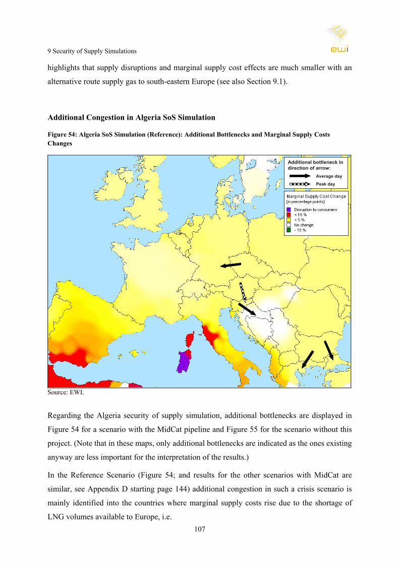
9 Security of Supply Simulations
107
highlights that supply disruptions and marginal supply cost effects are much smaller with an
alternative route supply gas to south-eastern Europe (see also Section 9.1).
Additional Congestion in Algeria SoS Simulation
Figure 54: Algeria SoS Simulation (Reference): Additional Bottlenecks and Marginal Supply Costs Changes
Additional bottleneck in direction of arrow:
Average day
Peak day
Source: EWI.
Regarding the Algeria security of supply simulation, additional bottlenecks are displayed in
Figure 54 for a scenario with the MidCat pipeline and Figure 55 for the scenario without this
project. (Note that in these maps, only additional bottlenecks are indicated as the ones existing
anyway are less important for the interpretation of the results.)
In the Reference Scenario (Figure 54; and results for the other scenarios with MidCat are
similar, see Appendix D starting page 144) additional congestion in such a crisis scenario is
mainly identified into the countries where marginal supply costs rise due to the shortage of
LNG volumes available to Europe, i.e.

9 Security of Supply Simulations
108
• from Austria to Slovenia to Croatia (Krk terminal),
• from Bulgaria to Greece and Turkey,
• and also from Austria into Italy (DG TREN Scenario).
The situation is different in the scenario without MidCat (South Stream Scenario, Figure 55):
As discussed previously, supply disruptions to consumers in Spain could then not be avoided,
even if the market worked as efficiently as presumed by the model assumptions. Hence, a
further bottleneck would become evident between France and Spain. Due to the supply dis-
ruptions in Spain in this scenario, the economic costs of congestion are relatively high then.
Figure 55: Algeria SoS Simulation (South Stream): Additional Bottlenecks and Marginal Supply Costs Changes
Additional bottleneck in direction of arrow:
Average day
Peak day
Source: EWI.
The results of this study with respect to security of supply also highlight the benefits of a
competitive gas market in general, and a liquid LNG market in particular, to natural gas
consumers in Europe. The simulated optimal responses to a crisis presume a functioning
9 Security of Supply Simulations
109
market which allows market players to actually implement these measures. Homogeneous and
efficient practices with respect to capacity allocation for both pipelines and LNG terminals in
Europe would reduce transaction costs and support the realisation of such efficient responses
in the gas market in case of a crisis. With respect to LNG, the results specifically show that
these volumes are of large importance for the whole European gas market – including
countries which do not import LNG – and support the mitigation of gas supply disruptions.
Hence, a flexible LNG supply market and the establishment of efficient (and harmonised)
LNG import capacity allocation mechanisms benefit consumers beyond the borders of the
LNG importing countries.
10 EWI Study in the Context of European Gas Infrastructure Analyses
110
10 EWI Study in the Context of European Gas Infrastructure Analyses
In 2009, ENTSOG (2009) published its European Ten Year Network Development Plan as
the first wide-ranging documentation on infrastructure (pipelines, LNG terminals, gas
storages), infrastructure projects, production deliverability and import capacities. Considering
those relative to an annual and a peak demand day scenario allows conclusions on the
sufficiency of capacities for the demand-capacity balances for each European country.
With respect to security of supply, European and regional analysis is currently being carried
out by the Pentalateral Energy Forum und the European Commission’s Gas Coordination
Group. However, work is still in progress with no results in the public domain yet.74 Country-
specific investigations of stress scenarios in the gas market on UK energy supply have been
published by Ofgem (2009).75
This ERGEG-initiated study is one of the first to investigate issues of gas flows, market
integration and security of supply with an encompassing model-based approach. The model
validation showed that the applied TIGER model is an appropriate tool for such an analysis
although some contract-induced gas flows cannot always be replicated. This approach allows
for the possibility to explicitly consider natural gas flows and volumes as published technical
capacities and interconnections of all relevant elements in the European gas transport infra-
structure are considered (further pipeline-operational issues are not).
In terms of results, the model-based analysis allows investigations which exceed the scope of
previous studies. However, the approach also confirms findings published by other
institutions.
With respect to ENTSOG (2009)76, EWI results are similar regarding the interconnection of
countries and supply-demand gaps:
• ENTSOG reports sufficient capacities to cover demand (including the peak demand day)
in Austria, Belgium, the Czech Republic, France, Germany, Ireland, Italy, Luxembourg,
the Netherlands, Switzerland and the United Kingdom. (Although this is not explicitly 74 The model the EU might apply to do so is presented by Monforti and Szikszaia (2010). 75 “Project Discovery”. 76 An interpretation and summary of results with respect to bottlenecks and security of supply is provided in ENTSOG (2010).

10 EWI Study in the Context of European Gas Infrastructure Analyses
111
stated by ENTSOG (2010), the same is true for all other considered countries except those
stated below (DK, SE, SI, HU, BA, MK, RS).)
• This study confirms ENTSOG’s findings. Additionally, the model-based approach also
allows the conclusion that there is not only sufficient capacity, but that the gas volumes
are also there to fill these capacities with natural gas (with one exception, see next
paragraph) in all considered scenarios, with different demand projections, and on the peak
demand day.
• Five of the six demand-capacity gaps identified by ENTSOG are also replicated by the
EWI study as demand-supply gaps, which is not surprising as capacity is a prerequisite for
the delivery of volumes. These concern the region of Denmark and Sweden, Hungary,
Bosnia and Herzegovina, Macedonia and Serbia. What are not replicated are demand-
supply gaps is in Slovenia which may be due to differing assumptions on LNG supplies to
neighbouring Croatia.77
Apart from the stress scenarios, this study exceeds the work by ENTSOG (2009) in two other
aspects: the variation of infrastructure assumptions between scenarios and the focus on gas
volumes (in addition to capacities) enabled by the model simulation. This allows further
conclusions:
• Potential demand-supply gaps are also a function of which new infrastructure projects are
realised. The study at hand shows that the demand-supply gaps in south-eastern Europe
are either reduced or fully eliminated if one of the major new import pipelines in the
region is assumed to be in place. This is true for Greece, Hungary, Bosnia and
Herzegovina and Serbia.
• In addition to the findings in line with ENTSOG outlined in the previous paragraph,
taking into account gas volumes produces further insights on supply-demand balances as
these volumes might not be available despite the capacity being there. This is found to be
relevant for one country, Greece, under certain circumstances: Even though sufficient
import capacity exists, high demand in Turkey might in some scenarios lead to a reduction
in Turkey-to-Greece gas flows causing a supply-demand gap in Greece when demand in 77 This study includes the Krk LNG terminal which then allows supplies from Croatia to Slovenia. Croatia is not explicitly considered in ENTSOG (2009).

10 EWI Study in the Context of European Gas Infrastructure Analyses
112
Greece is also very high (peak demand day). While this may be only relevant in the
extreme case of very high demand in both countries, it illustrates the importance of
considering both capacities and volumes.
Furthermore, the volume-based approach also allows for the identification of congestion on
pipeline routes. Hence, not only potential capacity issues leading to severe security of supply
issues (supply-demand gaps) can be identified. This analysis also enables us to determine
bottlenecks which limit market integration. Depending on the scenario and the considered
time of the year, such congestion was identified between:
• the UK and the continent (peak demand day only),
• Germany and France, Belgium and the Netherlands (peak demand day only),
• Austria, Slovenia, Croatia (depending on LNG prices and time of the year)
• the Slovak Republic and Austria,
• and, in the case of temporally low LNG prices, also partially between Spain and France,
France and Switzerland and Germany, Belgium and France, the Netherlands and
Germany, Germany and the Czech Republic, and Greece and Bulgaria.
All major points of congestion identified in this study are also depicted in Figure 56.78 The
map, thereby, also highlights the value-added provided by this study compared to, for
instance, capacity considerations as done by ENTSOG (2009): Such considerations are only
able to detect bottlenecks leading to demand-supply (or demand-capacity) gaps. The model-
based approach applied in this study, on the other hand, also enables the identification of
congestion which is not so severe as to cause demand disruptions, but that hampers market
integration. These kinds of bottlenecks are represented by the orange and blue arrows in
Figure 56; the red arrows represent different demand-capacity gap causing bottlenecks which
can be identified by a model-based as well as a capacity focused approach.
78 This only represents a simplification and aggregation of the bottlenecks for illustrative purpose. The scenario specific results are presented in Table 4 (page 66) in Section 8.2.

10 EWI Study in the Context of European Gas Infrastructure Analyses
113
Figure 56: Summary of bottlenecks in EWI Study
Supply-Demand gaps in all scenariosSupply-Demand gaps in some scenariosCongestion on pipelinesCongestion caused by “LNG Glut“
Source: EWI.
Regarding the security of supply stress scenarios, a classification of the EWI results in the
context of the other Europe-wide studies is not yet possible due to this study being the first
one to be published.
In the UK-focused analysis by Ofgem (2009), conclusions with respect to the UK are similar
although not perfectly comparable:
• A simulated 40 percent reduction in LNG imports leads to severe price effects and
demand reductions if it lasts for a whole 1-in-20 severe winter (Ofgem, 2009). This does
not contradict our finding that a temporary four-week-decline in LNG imports could be
compensated causing moderate effects on marginal supply costs and no demand
reductions. The higher price effects found by Ofgem (compared to this study) are the
consequence of the longer duration of the assumed LNG import reduction (whole winter
vs. four weeks).
10 EWI Study in the Context of European Gas Infrastructure Analyses
114
• With respect to a Russia-Ukraine dispute, Ofgem (2009) finds that the UK is well
protected against such a crisis unless investment in infrastructure (storages) is low. As the
study at hand presumes significant investments in storages in the UK, it can only be
compared to the Ofgem (2009) scenarios with higher investments and, hence, mirrors their
results that consequences in this case are rather small.
However, it has to be noted that focus and methodology of the studies differ.

Appendices
115
Bibliography
Baulch, B. (1997). Transfer Costs, Spatial Arbitrage, and Testing for Food Market
Integration. In: American Journal of Agricultural Economics, 79 (2), pp. 477-487.
Bettzüge, M.O. (2009). “Analysis of the January Gas Crisis & Implications for Security of
Gas Supply Regulations.” Presentation at Mini-Public Hearing on Security of Gas Supply at
the European Parliament, Brussels/Belgium, 9th November 2009. Download: http://www.
europarl.europa.eu/document/activities/cont/200911/20091118ATT64744/20091118ATT647
44EN.pdf (01/04/2010).
Bettzüge, M.O.; S. Lochner (2009). Der russisch-ukrainische Gaskonflikt im Januar 2009 –
eine modell-gestützte Analyse. [The Russian-Ukrainian Gas Conflict of January 2009 – a
model-based analysis.] In: Energiewirtschaftliche Tagesfragen, 59 (7), pp. 26-30. (in German
only)
BP (2009). BP Statistical Review of World Energy. London/UK.
De Vany, A.; W.D. Walls (1996). The Law of One Price in a Network: Arbitrage and Price
Dynamics in Natural Gas City Markets. In: Journal of Regional Science, 36 (4), pp. 555-570.
DowJones (2010). Shale-Gas: In Europa ist Euphorie noch verfrüht [European shale gas
euphoria yet too early]. DowJones TradeNews Energy, 2010 No. 69, 12 April 2010, p. 5.
Economist, The (2010). An unconventional glut. The Economist print edition, March 11th,
2010.
EIA (2009). International Energy Outlook. Energy Information Administration, Office of
Integrated Analysis and Forecasting, U.S. Department of Energy, Washington, DC/USA.
ENTSOG (2009). Ten Year Network Development Plan 2010 – 2019. Ref. 09-ENTSOG-002,
Brussels/Belgium, December 23, 2009. Download: http://www.entsog.eu/events/TYNDP1/
index.htm (28/02/2010).
ENTSOG (2010). ENTSOG European Ten Year Network Development Plan 2010-2019,
Presentation by Mr Volker Shippers, Brussels, January 26, 2010. Download:
Appendices
116
http://www.entsog.eu/download/TYNDR/presented/03_100126_1st_ENTSOG_TYNDP_WS
_Presentation_TYNDP_VS.ppt (25/02/2010).
European Commission (2008). European Energy and Transport – Trends to 2030, 2007
Update. Directorate-General for Energy and Transport, Brussels/Belgium.
European Commission (2009). Quarterly Report on the Euro Area, Focus II: “The Impact of
the economic and financial crisis on potential growth”, Directorate General for Economic and
Financial Affairs, Brussels/Belgium, p. 27.
EGM (2007). Focus on Storage. European Gas Markets 14-09 (2), Heren Energy, 28 Sep
2007, pp. 6-10.
EGM (2009). European Gas Market, ICIS Heren, 16-15, 24 Aug 2009.
EWI (2010). TIGER Infrastructure and Dispatch Model of the European Gas Market – Model
Description. Cologne/Germany. Download: http://www.ewi.uni-koeln.de/fileadmin/user/
PDFs/TIGER.pdf (28/02/2010).
GTE+ (2009): GTE+ Demand Scenarios vs. Capacity Report. Ref. 09GTE+144,
Brussels/Belgium, July 31, 2009. Download: http://www.gie.eu/events/gteplus/workshop/
tys3/download/090731_ GTEplus_DSCR.pdf (31/12/2009).
IEA (2008). World Energy Outlook, International Energy Agency, Paris/France.
IEA (2009). Natural Gas Information, International Energy Agency, Paris/France.
IGU (2006). UGS Data Bank. International Gas Union, Triennium 2003 – 2006, Working
Committee 2 - Underground Gas Storage. Download: http://www.igu.org/html/wgc2006/
WOC2database/index.htm (01/03/2010).
Lochner, S.; D. Bothe (2009). The development of natural gas supply costs to Europe, the
United States and Japan in a globalizing gas market - Model-based analysis until 2030. In:
Energy Policy, 37 (4), pp. 1518-1528.
Lochner (2009): Nodal prices, capacity valuation and investments in natural gas markets -
Overview and Analytical Framework. EWI Working Paper 09/2, Cologne/Germany.
Appendices
117
Lochner, S.; J. Richter (2010). The Impact of recent Gas Market Developments on long-term
Projections for Global Gas Supply. In: Zeitschrift für Energiewirtschaft, 34 (1), pp. 61-69.
Monforti, F.; A. Szikszaia (2010). A MonteCarlo approach for assessing the adequacy of the
European gas transmission system under supply crisis conditions. In: Energy Policy, 38 (5),
pp. 2486-2498.
Nabucco Gas Pipeline International GmbH (2009). Nabucco Gas Pipeline Project Website
http://www.nabucco-pipeline.com
Ofgem (2009). Project Discovery Energy Market Scenarios. Office of the Gas and Electricity
Markets, London/UK. Download: http://www.ofgem.gov.uk/MARKETS/WHLMKTS/
DISCOVERY/Documents1/Discovery_Scenarios_ConDoc_FINAL.pdf (25/02/2010).
OME (2001). Assessment of Internal and External Gas Supply Options for the EU, Evaluation
of the Supply Costs of New Natural Gas Supply Projects to the EU and an Investigation of
Related Financial Requirements and Tools. Chapter 3 - Assessment of Future Supply Costs to
Europe. Observatoire Méditerranéen de l’Énergie (OME), June 2001.
Petroleum Economist (2008). Gas in the CIS & Europe – 2008 edition. The Petroleum
Economist Ltd, June 2008, London/UK.
Pirani, S.; J. Stern and K. Yafimava (2009): The Russo-Ukrainian gas dispute of January
2009: a comprehensive assessment. Oxford Institute for Energy Studies, February 2009, NG
27.
Seeliger (2006). Entwicklung des weltweiten Erdgasangebots bis 2030 – Eine modellgestützte
Prognose [The development of global gas supply until 2030 – a model-based projection].
Oldenburg Verlag, Munich/Germany.
South Stream (2010). Gas Pipeline Project webpage http://south-stream.info
United Nations (1999). Study on Underground Gas Storage in Europe and Central Asia. UN
Economic Commission for Europe - Working Party on Gas.
WoodMackenzie (2008): LNG Service – Turkey Key Market Facts, September 2008.
Appendices
118
List of Legal Sources
COM (2009) 361: Proposal for a COUNCIL REGULATION concerning the notification to
the Commission of investment projects in energy infrastructure within the European
Community and repealing Regulation (EC) No 736/96.
COM (2009) 363: Proposal for a REGULATION OF THE EUROPEAN PARLIAMENT
AND OF THE COUNCIL concerning measures to safeguard security of gas supply and
repealing Directive 2004/67/EC.
Decision No 1364/2006/EC: Decision No 1364/2006/EC of 6 September 2006 laying down
guidelines for trans-European energy networks and repealing Decision 96/391/EC and
Decision No 1229/2003/EC.
Directive 2004/67/EC: Council Directive 2004/67/EC of 26 April 2004 concerning measures
to safeguard security of natural gas supply.
Directive 2009/73/EC: Directive 2009/73/EC of the European Parliament and of the Council
of 13 July 2009 concerning common rules for the internal market in natural gas and repealing
Directive 2003/55/EC.
Regulation (EC) No 713/2009: Regulation (EC) No 713/2009 of the European Parliament
and of the Council of 13 July 2009 establishing an Agency for the Cooperation of Energy
Regulators.
Regulation (EC) No 715/2009: Regulation (EC) No 715/2009 of the European Parliament
and of the Council of 13 July 2009 on conditions for access to the natural gas transmission
networks and repealing Regulation (EC) No 1775/2005.
2003/796/EC: Commission Decision of 11 November 2003 on establishing the European
Regulators Group for Electricity and Gas.
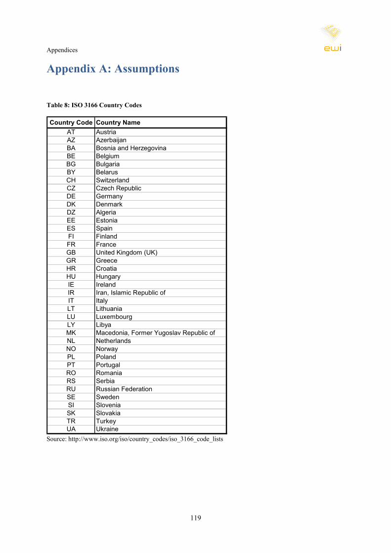
Appendices
119
Appendix A: Assumptions
Table 8: ISO 3166 Country Codes
Country Code Country NameAT AustriaAZ AzerbaijanBA Bosnia and HerzegovinaBE BelgiumBG BulgariaBY BelarusCH SwitzerlandCZ Czech RepublicDE GermanyDK DenmarkDZ AlgeriaEE EstoniaES SpainFI FinlandFR FranceGB United Kingdom (UK)GR GreeceHR CroatiaHU HungaryIE IrelandIR Iran, Islamic Republic ofIT ItalyLT LithuaniaLU LuxembourgLY LibyaMK Macedonia, Former Yugoslav Republic ofNL NetherlandsNO NorwayPL PolandPT PortugalRO RomaniaRS SerbiaRU Russian FederationSE SwedenSI SloveniaSK SlovakiaTR TurkeyUA Ukraine
Source: http://www.iso.org/iso/country_codes/iso_3166_code_lists

Appendices
120
Table 9: List of pipeline abbreviations
Pipeline (Project) Full Name Specification of RouteBBL Balgzand-Bacton-Line Balgzand (NL) - Bacton (GB)GALSI Gasdotto Algeria Sardegna Italia offshore section: Koudiet Draouche (DZ) -
Porto Botte, Sardinia (IT) - Piombino (IT)IGI (also Poseidon) Interconnector Greece-Italy offshore section: Igoumenitsa (GR) - Otranto (IT)Medgaz Mediterranean Gaz pipeline Hassi R'mel (DZ) - Almeida (ES)MEGAL Mittel-Europäische-Gasleitung Waidhaus (CZ-DE border) - Medelsheim (DE-FR border)
(2nd southern section from AT-DE border in Oberkappel)MidCat Midi – Cataluña Pipeline Project Barcelona region (Martorell, ES) - southern France
(Beziers) / (bi-directional)NEL Norddeutsche Erdgasleitung Lubmin (DE) - Achim (DE)OPAL Ostsee-Pipeline-Anbindungs-Leitung Lubmin (DE) - Olbernhau (DE-CZ border)TAG Trans Austria Gasleitung SK-AT border - Baumgarten (AT) - AT-IT borderTAP Trans-Adriatic Pipeline Thessaloniki (GR) - Albania - Puglia region (IT)TGL Tauerngasleitung Haiming (DE) - AT - Malborghetto/Tarvis (AT-IT border) /
(bi-directional)Transmed Trans-Mediterranean Pipeline Hassi R'mel (DZ) - Tunisia - Mazara del Vallo, Sicily (IT) Source: EWI.
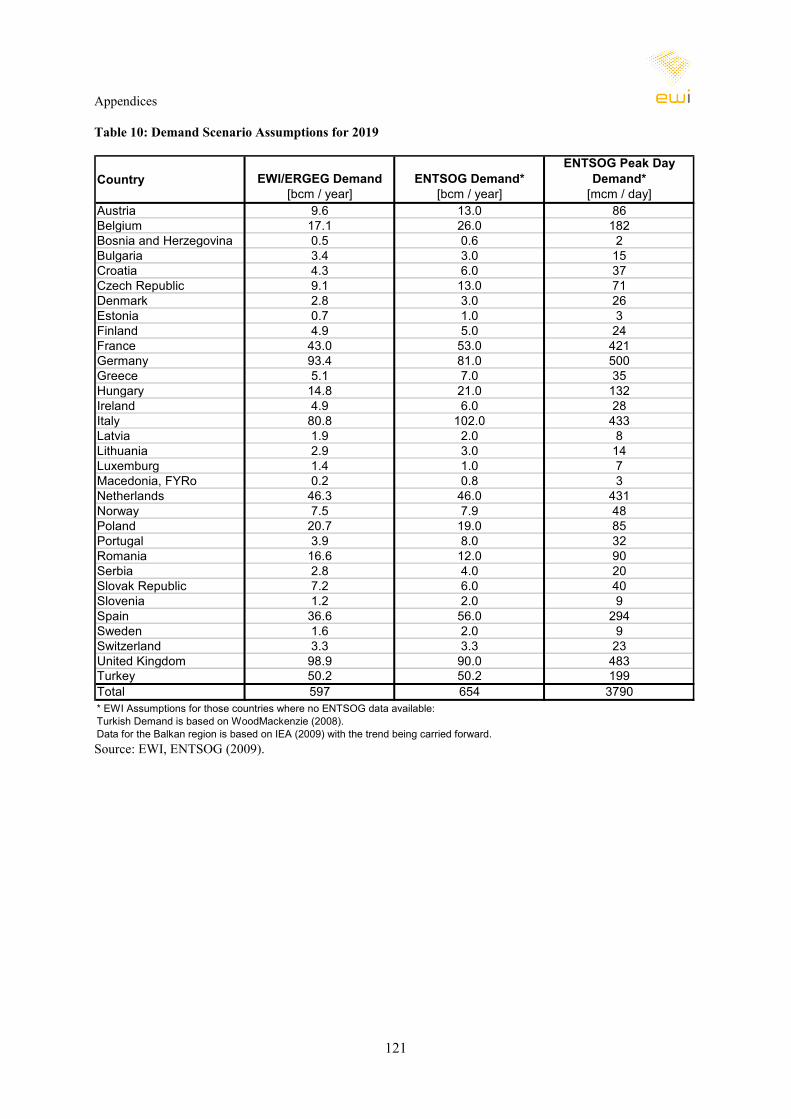
Appendices
121
Table 10: Demand Scenario Assumptions for 2019
Country EWI/ERGEG Demand[bcm / year]
ENTSOG Demand*[bcm / year]
ENTSOG Peak Day Demand*
[mcm / day]Austria 9.6 13.0 86Belgium 17.1 26.0 182Bosnia and Herzegovina 0.5 0.6 2Bulgaria 3.4 3.0 15Croatia 4.3 6.0 37Czech Republic 9.1 13.0 71Denmark 2.8 3.0 26Estonia 0.7 1.0 3Finland 4.9 5.0 24France 43.0 53.0 421Germany 93.4 81.0 500Greece 5.1 7.0 35Hungary 14.8 21.0 132Ireland 4.9 6.0 28Italy 80.8 102.0 433Latvia 1.9 2.0 8Lithuania 2.9 3.0 14Luxemburg 1.4 1.0 7Macedonia, FYRo 0.2 0.8 3Netherlands 46.3 46.0 431Norway 7.5 7.9 48Poland 20.7 19.0 85Portugal 3.9 8.0 32Romania 16.6 12.0 90Serbia 2.8 4.0 20Slovak Republic 7.2 6.0 40Slovenia 1.2 2.0 9Spain 36.6 56.0 294Sweden 1.6 2.0 9Switzerland 3.3 3.3 23United Kingdom 98.9 90.0 483Turkey 50.2 50.2 199Total 597 654 3790* EWI Assumptions for those countries where no ENTSOG data available: Turkish Demand is based on WoodMackenzie (2008). Data for the Balkan region is based on IEA (2009) with the trend being carried forward. Source: EWI, ENTSOG (2009).
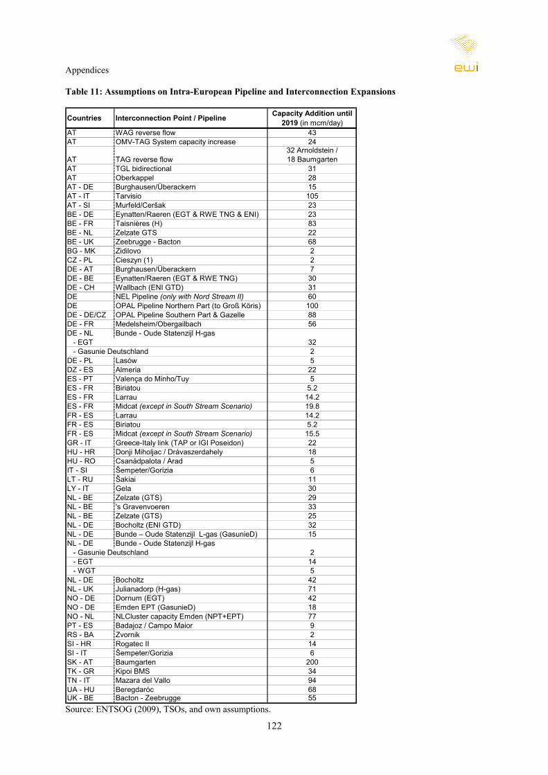
Appendices
122
Table 11: Assumptions on Intra-European Pipeline and Interconnection Expansions
Countries Interconnection Point / Pipeline Capacity Addition until 2019 (in mcm/day)
AT WAG reverse flow 43AT OMV-TAG System capacity increase 24
AT TAG reverse flow32 Arnoldstein /18 Baumgarten
AT TGL bidirectional 31AT Oberkappel 28AT - DE Burghausen/Überackern 15AT - IT Tarvisio 105AT - SI Murfeld/Ceršak 23BE - DE Eynatten/Raeren (EGT & RWE TNG & ENI) 23BE - FR Taisnières (H) 83BE - NL Zelzate GTS 22BE - UK Zeebrugge - Bacton 68BG - MK Zidilovo 2CZ - PL Cieszyn (1) 2DE - AT Burghausen/Überackern 7DE - BE Eynatten/Raeren (EGT & RWE TNG) 30DE - CH Wallbach (ENI GTD) 31DE NEL Pipeline (only with Nord Stream II) 60DE OPAL Pipeline Northern Part (to Groß Köris) 100DE - DE/CZ OPAL Pipeline Southern Part & Gazelle 88DE - FR Medelsheim/Obergailbach 56DE - NL Bunde - Oude Statenzijl H-gas
- EGT 32- Gasunie Deutschland 2
DE - PL Lasów 5DZ - ES Almeria 22ES - PT Valença do Minho/Tuy 5ES - FR Biriatou 5.2ES - FR Larrau 14.2ES - FR Midcat (except in South Stream Scenario) 19.8FR - ES Larrau 14.2FR - ES Biriatou 5.2FR - ES Midcat (except in South Stream Scenario) 15.5GR - IT Greece-Italy link (TAP or IGI Poseidon) 22HU - HR Donji Miholjac / Drávaszerdahely 18HU - RO Csanádpalota / Arad 5IT - SI Šempeter/Gorizia 6LT - RU Šakiai 11LY - IT Gela 30NL - BE Zelzate (GTS) 29NL - BE 's Gravenvoeren 33NL - BE Zelzate (GTS) 25NL - DE Bocholtz (ENI GTD) 32NL - DE Bunde – Oude Statenzijl L-gas (GasunieD) 15NL - DE Bunde - Oude Statenzijl H-gas
- Gasunie Deutschland 2- EGT 14- WGT 5
NL - DE Bocholtz 42NL - UK Julianadorp (H-gas) 71NO - DE Dornum (EGT) 42NO - DE Emden EPT (GasunieD) 18NO - NL NLCluster capacity Emden (NPT+EPT) 77PT - ES Badajoz / Campo Maior 9RS - BA Zvornik 2SI - HR Rogatec II 14SI - IT Šempeter/Gorizia 6SK - AT Baumgarten 200TK - GR Kipoi BMS 34TN - IT Mazara del Vallo 94UA - HU Beregdaróc 68UK - BE Bacton - Zeebrugge 55 Source: ENTSOG (2009), TSOs, and own assumptions.

Appendices
123
Table 12: Assumptions on Storage Projects / Expansions
Coun-try Name of facility Type of
facility Comment WGV* (mcm) Start-up Status
AT Haidach Reservoir New facility 1200 2011 Under construction
ATSchonkirchen Tief (Phase I) Reservoir New facility 850 2014 Planned
ATSchonkirchen Tief (Phase II) Reservoir New facility 750 2018 Planned
AT 7fields Reservoir New facility 1155 Apr 2011 PlannedAT 7fields Reservoir New facility 570 Apr 2014 PlannedBE Loenhout Aquifer Expansion 100 2010 Under constructionBG Chiren Reservoir Expansion 450 2010 Planned
FRCéré La Ronde/Soings Aquifer Expansion 400 2012 Under construction
FR Etrez Salt cavity Expansion 400 2015 Under ConstructionFR Etrez/Manosque Salt cavity Expansion 100 April 2008 LiveFR Hauterives Salt cavity New facility 150 2017 (full cap) Committed
FRIle-de-France Nord/Gournay Aquifer Expansion 500 2013 Under construction
FR Lussagnet / Izaute Aquifer Expansion 1100 2018 +100mcm/yearFR Manosque Salt cavity Expansion 130 2015 Under StudyFR Pécorade Reservoir New facility 750 2015 PlannedFR Trois Fontaines depleted field New facility 80 2010 Under ConstructionDE Bierwang depleted field Expansion 359 2015 under constructionDE Empelde Salt cavity New facility 110 2015 PlannedDE Epe Salt cavity New facility 200 2011 Under developmentDE Epe EGS H-Gas Salt cavity Expansion 273 2011 under constructionDE Epe Eneco Salt cavity New facility 100 2013 under constructionDE Epe Nuon Salt cavity Expansion 80 2011 under construction
DEEtzel EGL (share EGS) Salt cavity Expansion 250 2011 under construction
DE Etzel EGS Salt cavity New facility 2500 2016 Planned/CommittedDE Huntorf Salt cavity New facility 150 2015 PlannedDE Jemgum Salt cavity New facility 1200 2012 PlannedDE Kiel-Rönne Salt cavity New facility 70 2015 PlannedDE Krummhörn Salt cavity Reparation 229 2011 under constructionDE Peckensen Phase 2 Salt cavity New facility 160 2010 Under constructionDE Peckensen Phase 3 Salt cavity New facility 180 2014 CommittedDE Reckrod Salt cavity New facility 30 2015 PlannedDE Reckrod-Walf Salt cavity New facility 120 2015 PlannedDE Ruedersdorf Salt cavity New facility 300 2015 Under constructionDE Wolfersberg Reservoir Expansion 45 2010 PlannedDE Xanten Salt cavity Expansion 125 2015 PlannedHU Szoereg-1 Reservoir New facility 1900 2010 Under constructionHU Zsana Reservoir Expansion 600 late 2009 Under constructionIT Bordolano Reservoir New facility 1500 2013 Under constructionIT Caleppio-Merlino Reservoir New facility 450 2013 Under constructionIT Cellino & Collato Reservoir Expansion 552 2010 Under constructionIT Cignone Reservoir New facility 200 2013 CommittedIT Cornegliano Reservoir New facility 600 2015 Planned
IT Cotignola & San Potito Reservoir New facility 915 2013 Committed

Appendices
124
(continued)
Country Name of facility Type of
facility Comment WGV* (mcm) Start-up Status
IT Cugno Le Macine Reservoir New facility 740 2015 PlannedIT Fiume Treste BCC1 Reservoir New facility 350 2010 Under constructionIT Fiume Treste C2 Reservoir Expansion 200 2010 Under constructionIT Fiume Treste DEE0 Reservoir New facility 600 2010 Under constructionIT Ripalta Reservoir Expansion 300 2010 Under constructionIT Rivara Aquifer New facility 3000 2013 PlannedIT Sergnano Reservoir Expansion 200 2010 Under constructionLV Incukalns Reservoir Expansion 1000 2015 PlannedNL Bergermeer Reservoir New facility 4100 2013 PlannedNL Zuidwending Salt cavity New facility 180 2011 Under constructionPL Bonikowo Reservoir New facility 200 2010 CommittedPL Daszewo Reservoir New facility 30 2010 Under constructionPL Kosakowo Salt cavity New facility 250 2018 CommittedPL Mogilno Salt cavity Expansion 420 2018 Under constructionPL Strachocina Reservoir Expansion 180 2012 CommittedRS Banatski Dvor Reservoir New facility 800ES El Ruedo Reservoir New facility 90 2011 CommittedES Gaviota Reservoir Expansion 570 2015 CommittedES Las Barreras Reservoir New facility 72 2011 CommittedES Marismas Reservoir New facility 300 2011 CommittedES Marismas Reservoir New facility 300 2013 CommittedES Poseidon Reservoir New facility 250 2010 CommittedES Yela Aquifer New facility 1050 2011 Under constructionTR Tuz Gölü Reservoir New facility 1000 2015 CommittedGB Albury Phase 1 Reservoir New facility 160 2018 PlannedGB Aldbrough phase 2 Salt cavity Expansion 150 2013 PlannedGB Bains Offshore ReservNew facility 570 2013 PlannedGB Baird Offshore ReservNew facility 136 2016 PlannedGB Bletchingley Salt cavity New facility 605 2010 PlannedGB British Salt Salt Cavity New facility 1000 2016 PlannedGB Caythorpe Reservoir New facility 200 2011 PlannedGB Esmond / Gordon Offshore reserv New facility 4100 2015 PlannedGB Fleetwood Salt cavity New facility 1700 2018 PlannedGB Gateway Salt cavity New facility 1136 2019 PlannedGB Hewett Offshore ReservNew facility 5000 2015 PlannedGB Hole House phase 2 Salt cavity Expansion 27 2010 Under construction
GBHolford (formerly Byley) Salt cavity New facility 170 2011 Under construction
GB Isle of Portland Salt Cavity New facility 330 2015 PlannedGB Saltfleetby Reservoir New facility 600 2011 PlannedGB Stublach Salt cavity New facility 400 2013 Under construction
GBWelton / Scampton North Reservoir New facility 435 2018 Planned
GB Whitehill Farm Salt cavity New facility 420 2018 Planned
* Working Gas Volume for Expansion refers to additional WGV (not total WGV after expansion). Source: Own assumptions, GSE, IGU (2006) and EGM (2007).
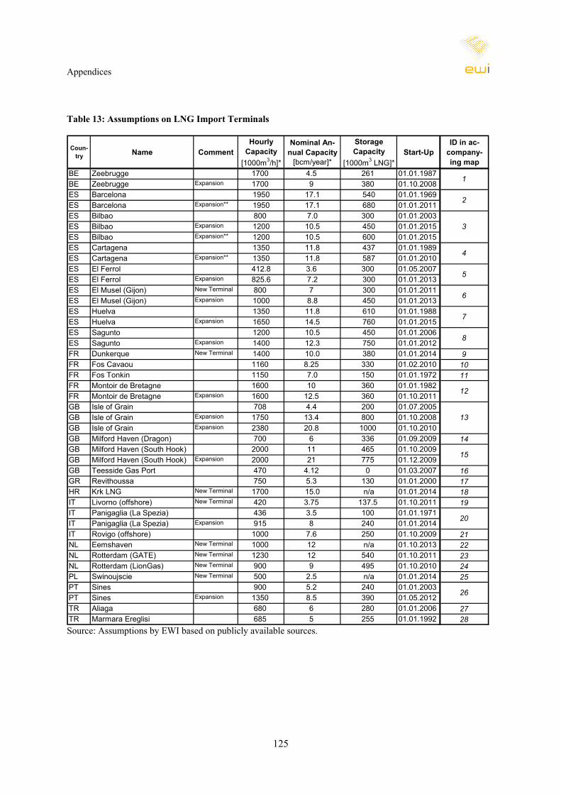
Appendices
125
Table 13: Assumptions on LNG Import Terminals
Coun-try Name Comment
Hourly Capacity
[1000m3/h]*
Nominal An-nual Capacity
[bcm/year]*
Storage Capacity
[1000m3 LNG]*Start-Up
ID in ac-company-ing map
BE Zeebrugge 1700 4.5 261 01.01.1987 BE Zeebrugge Expansion 1700 9 380 01.10.2008 ES Barcelona 1950 17.1 540 01.01.1969 ES Barcelona Expansion** 1950 17.1 680 01.01.2011ES Bilbao 800 7.0 300 01.01.2003ES Bilbao Expansion 1200 10.5 450 01.01.2015ES Bilbao Expansion** 1200 10.5 600 01.01.2015ES Cartagena 1350 11.8 437 01.01.1989 ES Cartagena Expansion** 1350 11.8 587 01.01.2010ES El Ferrol 412.8 3.6 300 01.05.2007ES El Ferrol Expansion 825.6 7.2 300 01.01.2013ES El Musel (Gijon) New Terminal 800 7 300 01.01.2011 ES El Musel (Gijon) Expansion 1000 8.8 450 01.01.2013ES Huelva 1350 11.8 610 01.01.1988 ES Huelva Expansion 1650 14.5 760 01.01.2015ES Sagunto 1200 10.5 450 01.01.2006ES Sagunto Expansion 1400 12.3 750 01.01.2012FR Dunkerque New Terminal 1400 10.0 380 01.01.2014 9FR Fos Cavaou 1160 8.25 330 01.02.2010 10FR Fos Tonkin 1150 7.0 150 01.01.1972 11FR Montoir de Bretagne 1600 10 360 01.01.1982FR Montoir de Bretagne Expansion 1600 12.5 360 01.10.2011GB Isle of Grain 708 4.4 200 01.07.2005GB Isle of Grain Expansion 1750 13.4 800 01.10.2008GB Isle of Grain Expansion 2380 20.8 1000 01.10.2010GB Milford Haven (Dragon) 700 6 336 01.09.2009 14GB Milford Haven (South Hook) 2000 11 465 01.10.2009GB Milford Haven (South Hook) Expansion 2000 21 775 01.12.2009GB Teesside Gas Port 470 4.12 0 01.03.2007 16GR Revithoussa 750 5.3 130 01.01.2000 17HR Krk LNG New Terminal 1700 15.0 n/a 01.01.2014 18IT Livorno (offshore) New Terminal 420 3.75 137.5 01.10.2011 19IT Panigaglia (La Spezia) 436 3.5 100 01.01.1971 IT Panigaglia (La Spezia) Expansion 915 8 240 01.01.2014 IT Rovigo (offshore) 1000 7.6 250 01.10.2009 21NL Eemshaven New Terminal 1000 12 n/a 01.10.2013 22NL Rotterdam (GATE) New Terminal 1230 12 540 01.10.2011 23NL Rotterdam (LionGas) New Terminal 900 9 495 01.10.2010 24PL Swinoujscie New Terminal 500 2.5 n/a 01.01.2014 25PT Sines 900 5.2 240 01.01.2003 PT Sines Expansion 1350 8.5 390 01.05.2012 TR Aliaga 680 6 280 01.01.2006 27TR Marmara Ereglisi 685 5 255 01.01.1992 28
1
5
4
3
2
12
8
7
6
20
26
15
13
Source: Assumptions by EWI based on publicly available sources.
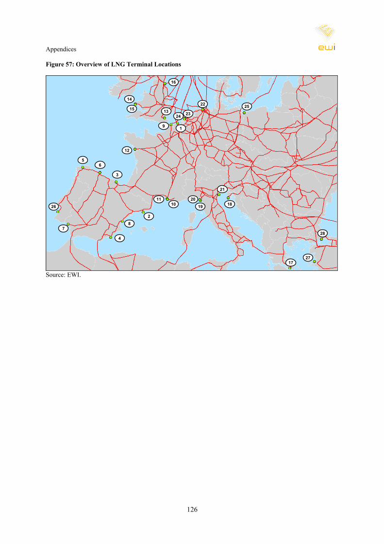
Appendices
126
Figure 57: Overview of LNG Terminal Locations
1
2
3
4
26
56
78
9
1011
12
13
14
16
15
17
181920
21
22
2324
25
27
28
Source: EWI.

Appendices
127
Appendix B: Additional Gas Flow Charts
Figure 58: Annual Gas Flows 2019 – Reference Scenario (ENTSOG Demand)
Yamal
Nord Stre
am
GALSIMedgaz
Transgas
Yamal
Nord Stre
am
GALSIMedgaz
Transgas
Source: EWI.
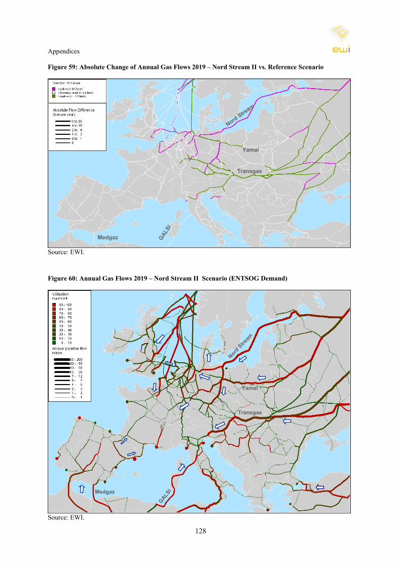
Appendices
128
Figure 59: Absolute Change of Annual Gas Flows 2019 – Nord Stream II vs. Reference Scenario
Yamal
Nord Stream
Medgaz
Transgas
GALSI
Source: EWI.
Figure 60: Annual Gas Flows 2019 – Nord Stream II Scenario (ENTSOG Demand)
Yamal
Nord Stre
am
GALSIMedgaz
Transgas
Yamal
Nord Stre
am
GALSIMedgaz
Transgas
Source: EWI.
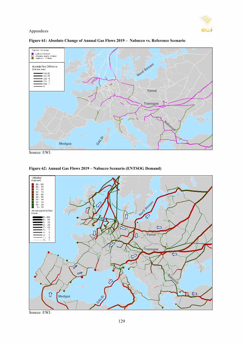
Appendices
129
Figure 61: Absolute Change of Annual Gas Flows 2019 – Nabucco vs. Reference Scenario
Yamal
Nord Stream
Medgaz
Nabucco
Transgas
GALSI
Source: EWI.
Figure 62: Annual Gas Flows 2019 – Nabucco Scenario (ENTSOG Demand)
Yamal
Nord Stre
am
GALSIMedgaz
Nabucco
Transgas
Yamal
Nord Stre
am
GALSIMedgaz
Nabucco
Transgas
Source: EWI.
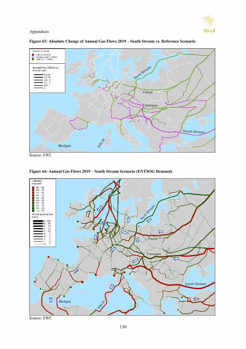
Appendices
130
Figure 63: Absolute Change of Annual Gas Flows 2019 – South Stream vs. Reference Scenario
Yamal
Nord Stream
Medgaz
South Stream
Transgas
GALSI
Source: EWI.
Figure 64: Annual Gas Flows 2019 – South Stream Scenario (ENTSOG Demand)
Yamal
Nord Stre
am
GALSIMedgaz
South Stream
Transgas
Yamal
Nord Stre
am
GALSIMedgaz
South Stream
Transgas
Source: EWI.

Appendices
131
Figure 65: Absolute Change of Annual Gas Flows 2019 – DG TREN vs. Reference Scenario
Yamal
Nord Stream
GALSI
Medgaz
Nabucco
Transgas
Source: EWI.
Figure 66: Annual Gas Flows 2019 – DG TREN Scenario (ENTSOG Demand)
Yamal
Nord Stre
am
GALSIMedgaz
Nabucco
Transgas
Yamal
Nord Stre
am
GALSIMedgaz
Nabucco
Transgas
Source: EWI.
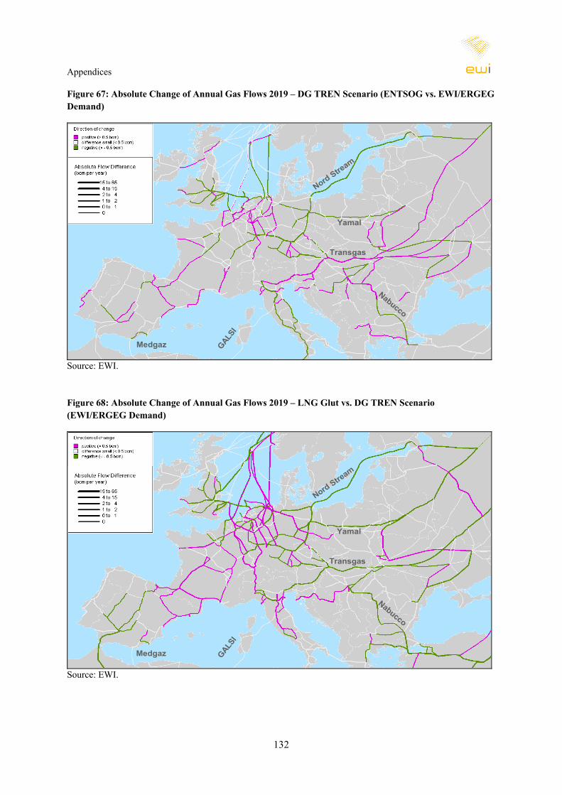
Appendices
132
Figure 67: Absolute Change of Annual Gas Flows 2019 – DG TREN Scenario (ENTSOG vs. EWI/ERGEG Demand)
Yamal
Nord Stream
Medgaz
Nabucco
Transgas
GALSI
Source: EWI.
Figure 68: Absolute Change of Annual Gas Flows 2019 – LNG Glut vs. DG TREN Scenario (EWI/ERGEG Demand)
Yamal
Nord Stream
Medgaz
Nabucco
Transgas
GALSI
Source: EWI.
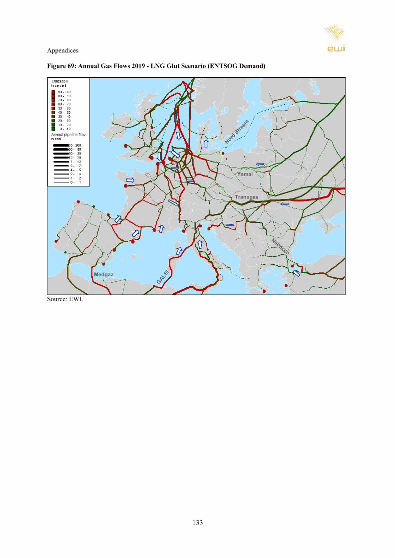
Appendices
133
Figure 69: Annual Gas Flows 2019 - LNG Glut Scenario (ENTSOG Demand)
Yamal
Nord Stre
am
GALSIMedgaz
Nabucco
Transgas
Source: EWI.
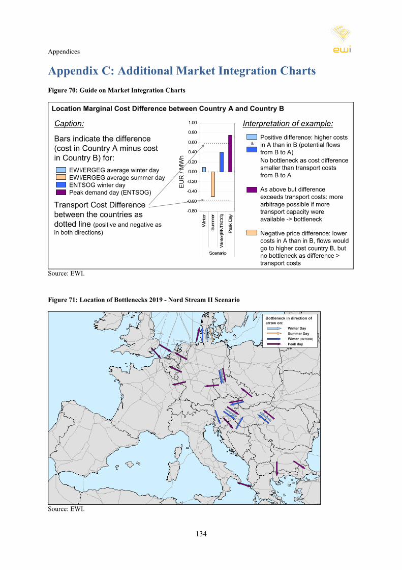
Appendices
134
Appendix C: Additional Market Integration Charts Figure 70: Guide on Market Integration Charts
-0.80
-0.60
-0.40
-0.20
0.00
0.20
0.40
0.60
0.80
1.00
Win
ter
Sum
mer
Win
ter(E
NTS
OG
)
Pea
k D
ay
Scenario
EU
R /
MW
h
Location Marginal Cost Difference between Country A and Country B
Bars indicate the difference (cost in Country A minus cost in Country B) for:
EWI/ERGEG average winter dayEWI/ERGEG average summer dayENTSOG winter dayPeak demand day (ENTSOG)
Transport Cost Difference between the countries as dotted line (positive and negative as in both directions)
Interpretation of example:Positive difference: higher costs in A than in B (potential flows from B to A)No bottleneck as cost difference smaller than transport costs from B to A
As above but difference exceeds transport costs: more arbitrage possible if more transport capacity were available -> bottleneck
Negative price difference: lower costs in A than in B, flows would go to higher cost country B, but no bottleneck as difference > transport costs
&
Caption:
Source: EWI.
Figure 71: Location of Bottlenecks 2019 - Nord Stream II Scenario
Bottleneck in direction of arrow on:
Winter DaySummer DayWinter (ENTSOG)
Peak day
Source: EWI.
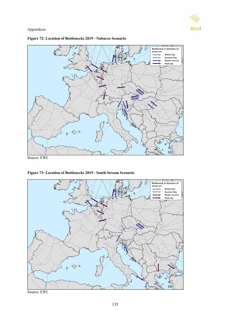
Appendices
135
Figure 72: Location of Bottlenecks 2019 - Nabucco Scenario
Bottleneck in direction of arrow on:
Winter DaySummer DayWinter (ENTSOG)
Peak day
Source: EWI.
Figure 73: Location of Bottlenecks 2019 - South Stream Scenario
Bottleneck in direction of arrow on:
Winter DaySummer DayWinter (ENTSOG)
Peak day
Source: EWI.
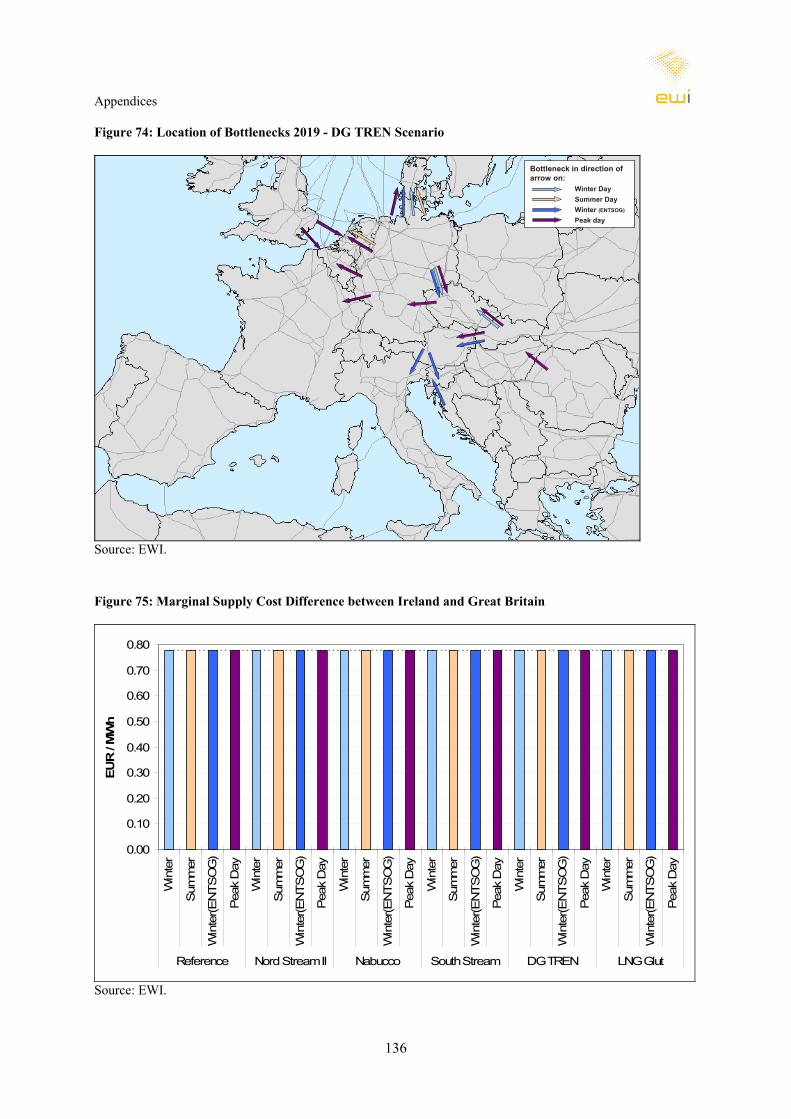
Appendices
136
Figure 74: Location of Bottlenecks 2019 - DG TREN Scenario
Bottleneck in direction of arrow on:
Winter DaySummer DayWinter (ENTSOG)
Peak day
Source: EWI.
Figure 75: Marginal Supply Cost Difference between Ireland and Great Britain
0.00
0.10
0.20
0.30
0.40
0.50
0.60
0.70
0.80
Win
ter
Sum
mer
Win
ter(E
NTS
OG
)
Pea
k D
ay
Win
ter
Sum
mer
Win
ter(E
NTS
OG
)
Pea
k D
ay
Win
ter
Sum
mer
Win
ter(E
NTS
OG
)
Pea
k D
ay
Win
ter
Sum
mer
Win
ter(E
NTS
OG
)
Pea
k D
ay
Win
ter
Sum
mer
Win
ter(E
NTS
OG
)
Pea
k D
ay
Win
ter
Sum
mer
Win
ter(E
NTS
OG
)
Pea
k D
ay
Reference Nord Stream II Nabucco South Stream DG TREN LNG Glut
EUR
/ M
Wh
Source: EWI.
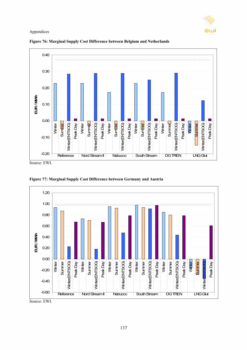
Appendices
137
Figure 76: Marginal Supply Cost Difference between Belgium and Netherlands
-0.20
-0.10
0.00
0.10
0.20
0.30
0.40W
inte
r
Sum
mer
Win
ter(E
NTS
OG
)
Pea
k D
ay
Win
ter
Sum
mer
Win
ter(E
NTS
OG
)
Pea
k D
ay
Win
ter
Sum
mer
Win
ter(E
NTS
OG
)
Pea
k D
ay
Win
ter
Sum
mer
Win
ter(E
NTS
OG
)
Pea
k D
ay
Win
ter
Sum
mer
Win
ter(E
NTS
OG
)
Pea
k D
ay
Win
ter
Sum
mer
Win
ter(E
NTS
OG
)
Pea
k D
ay
Reference Nord Stream II Nabucco South Stream DG TREN LNG Glut
EUR
/ M
Wh
Source: EWI.
Figure 77: Marginal Supply Cost Difference between Germany and Austria
-0.60
-0.40
-0.20
0.00
0.20
0.40
0.60
0.80
1.00
1.20
Win
ter
Sum
mer
Win
ter(E
NTS
OG
)
Pea
k D
ay
Win
ter
Sum
mer
Win
ter(E
NTS
OG
)
Pea
k D
ay
Win
ter
Sum
mer
Win
ter(E
NTS
OG
)
Pea
k D
ay
Win
ter
Sum
mer
Win
ter(E
NTS
OG
)
Pea
k D
ay
Win
ter
Sum
mer
Win
ter(E
NTS
OG
)
Pea
k D
ay
Win
ter
Sum
mer
Win
ter(E
NTS
OG
)
Pea
k D
ay
Reference Nord Stream II Nabucco South Stream DG TREN LNG Glut
EUR
/ M
Wh
Source: EWI.
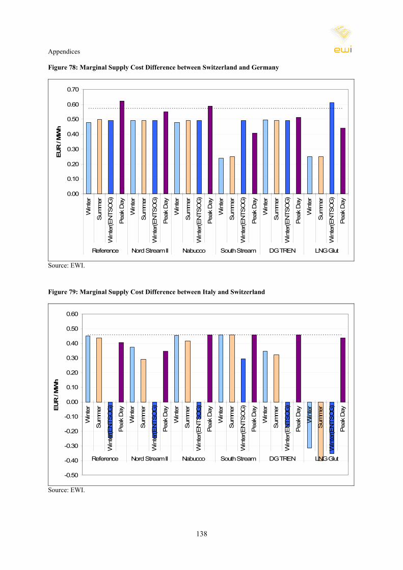
Appendices
138
Figure 78: Marginal Supply Cost Difference between Switzerland and Germany
0.00
0.10
0.20
0.30
0.40
0.50
0.60
0.70W
inte
r
Sum
mer
Win
ter(E
NTS
OG
)
Pea
k D
ay
Win
ter
Sum
mer
Win
ter(E
NTS
OG
)
Pea
k D
ay
Win
ter
Sum
mer
Win
ter(E
NTS
OG
)
Pea
k D
ay
Win
ter
Sum
mer
Win
ter(E
NTS
OG
)
Pea
k D
ay
Win
ter
Sum
mer
Win
ter(E
NTS
OG
)
Pea
k D
ay
Win
ter
Sum
mer
Win
ter(E
NTS
OG
)
Pea
k D
ay
Reference Nord Stream II Nabucco South Stream DG TREN LNG Glut
EUR
/ M
Wh
Source: EWI.
Figure 79: Marginal Supply Cost Difference between Italy and Switzerland
-0.50
-0.40
-0.30
-0.20
-0.10
0.00
0.10
0.20
0.30
0.40
0.50
0.60
Win
ter
Sum
mer
Win
ter(E
NTS
OG
)
Pea
k D
ay
Win
ter
Sum
mer
Win
ter(E
NTS
OG
)
Pea
k D
ay
Win
ter
Sum
mer
Win
ter(E
NTS
OG
)
Pea
k D
ay
Win
ter
Sum
mer
Win
ter(E
NTS
OG
)
Pea
k D
ay
Win
ter
Sum
mer
Win
ter(E
NTS
OG
)
Pea
k D
ay
Win
ter
Sum
mer
Win
ter(E
NTS
OG
)
Pea
k D
ay
Reference Nord Stream II Nabucco South Stream DG TREN LNG Glut
EUR
/ M
Wh
Source: EWI.
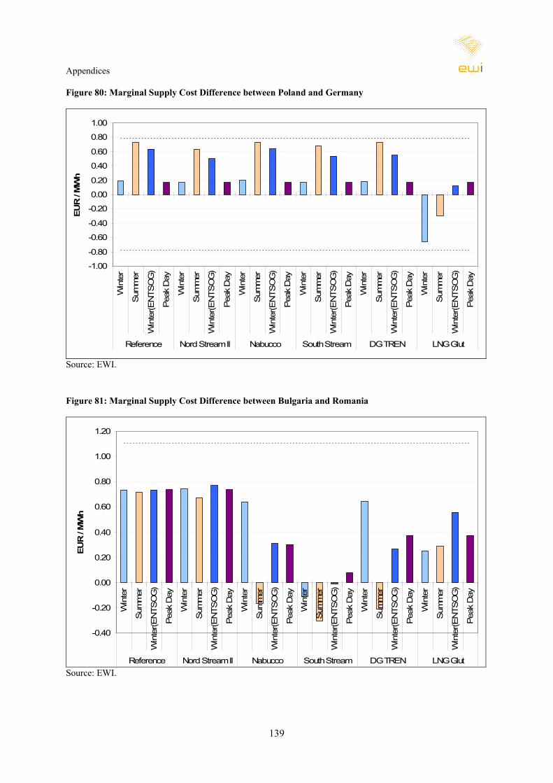
Appendices
139
Figure 80: Marginal Supply Cost Difference between Poland and Germany
-1.00
-0.80
-0.60
-0.40
-0.20
0.00
0.20
0.40
0.60
0.80
1.00W
inte
r
Sum
mer
Win
ter(E
NTS
OG
)
Pea
k D
ay
Win
ter
Sum
mer
Win
ter(E
NTS
OG
)
Pea
k D
ay
Win
ter
Sum
mer
Win
ter(E
NTS
OG
)
Pea
k D
ay
Win
ter
Sum
mer
Win
ter(E
NTS
OG
)
Pea
k D
ay
Win
ter
Sum
mer
Win
ter(E
NTS
OG
)
Pea
k D
ay
Win
ter
Sum
mer
Win
ter(E
NTS
OG
)
Pea
k D
ay
Reference Nord Stream II Nabucco South Stream DG TREN LNG Glut
EUR
/ M
Wh
Source: EWI.
Figure 81: Marginal Supply Cost Difference between Bulgaria and Romania
-0.40
-0.20
0.00
0.20
0.40
0.60
0.80
1.00
1.20
Win
ter
Sum
mer
Win
ter(E
NTS
OG
)
Pea
k D
ay
Win
ter
Sum
mer
Win
ter(E
NTS
OG
)
Pea
k D
ay
Win
ter
Sum
mer
Win
ter(E
NTS
OG
)
Pea
k D
ay
Win
ter
Sum
mer
Win
ter(E
NTS
OG
)
Pea
k D
ay
Win
ter
Sum
mer
Win
ter(E
NTS
OG
)
Pea
k D
ay
Win
ter
Sum
mer
Win
ter(E
NTS
OG
)
Pea
k D
ay
Reference Nord Stream II Nabucco South Stream DG TREN LNG Glut
EUR
/ M
Wh
Source: EWI.

Appendices
140
Figure 82: Marginal Supply Cost Difference between Turkey and Bulgaria
-1.00
0.00
1.00
2.00
3.00
4.00
5.00
6.00
7.00W
inte
r
Sum
mer
Win
ter(E
NTS
OG
)
Pea
k D
ay
Win
ter
Sum
mer
Win
ter(E
NTS
OG
)
Pea
k D
ay
Win
ter
Sum
mer
Win
ter(E
NTS
OG
)
Pea
k D
ay
Win
ter
Sum
mer
Win
ter(E
NTS
OG
)
Pea
k D
ay
Win
ter
Sum
mer
Win
ter(E
NTS
OG
)
Pea
k D
ay
Win
ter
Sum
mer
Win
ter(E
NTS
OG
)
Pea
k D
ay
Reference Nord Stream II Nabucco South Stream DG TREN LNG Glut
EUR
/ M
Wh
Source: EWI.
Figure 83: Marginal Supply Cost Difference between Turkey and Greece
-2.00
-1.50
-1.00
-0.50
0.00
0.50
1.00
1.50
2.00
Win
ter
Sum
mer
Win
ter(E
NTS
OG
)
Pea
k D
ay
Win
ter
Sum
mer
Win
ter(E
NTS
OG
)
Pea
k D
ay
Win
ter
Sum
mer
Win
ter(E
NTS
OG
)
Pea
k D
ay
Win
ter
Sum
mer
Win
ter(E
NTS
OG
)
Pea
k D
ay
Win
ter
Sum
mer
Win
ter(E
NTS
OG
)
Pea
k D
ay
Win
ter
Sum
mer
Win
ter(E
NTS
OG
)
Pea
k D
ay
Reference Nord Stream II Nabucco South Stream DG TREN LNG Glut
EUR
/ M
Wh
Source: EWI.

Appendices
141
Appendix D: Security of Supply Sensitivities – Further data
Table 14: Decline in LNG Imports in Algeria SoS Stress Simulation in mcm/day
Country Reference Nord Stream II Nabucco South Stream DG TRENGB -62.2 -65.8 -67.7 -49.0 -69.2BE -23.4 -23.1 -24.1 -4.9 -24.1NL -21.0 -18.2 -2.3 -54.0 -1.7FR -26.8 -27.3 -19.8 -20.5 -9.5ES -16.5 -13.9 -18.3 -18.1 -20.3PT -3.5 -3.4 -3.7 -3.5 -3.7IT -7.6 -7.6 -7.6 -7.6 -7.6
GR 0.0 0.0 0.3 -1.4 -0.2TR -6.4 -8.5 -5.7 -2.4 -5.9HR 0.0 0.0 -1.7 -12.6 -4.9
Source: EWI.
Figure 84: Bottlenecks and Marginal Cost Changes in Nord Stream II - Ukraine SoS Simulation
RR
Bottleneck in directionof arrow:
Average day
Peak day
(Grey colour impliesbottleneck also found in simulation withoutdisruption, see Chapter 8)
Source: EWI.
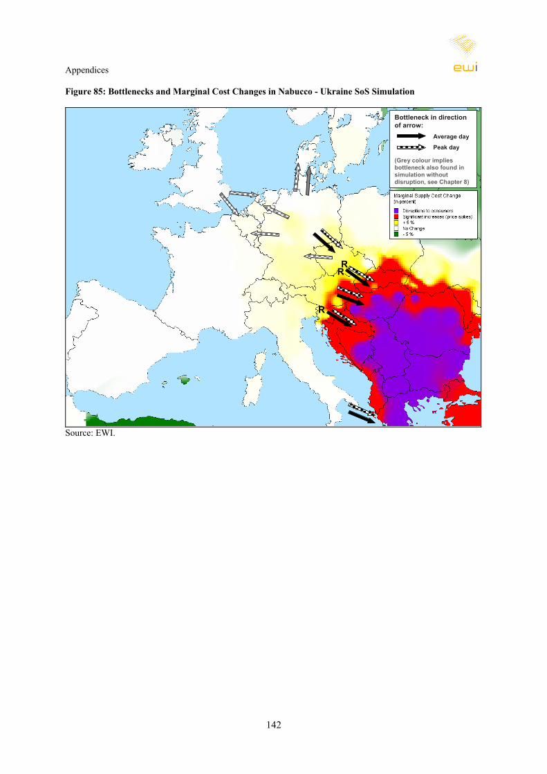
Appendices
142
Figure 85: Bottlenecks and Marginal Cost Changes in Nabucco - Ukraine SoS Simulation
RR
R
Bottleneck in directionof arrow:
Average day
Peak day
(Grey colour impliesbottleneck also found in simulation withoutdisruption, see Chapter 8)
Source: EWI.

Appendices
143
Figure 86: Bottlenecks and Marginal Cost Changes in DG TREN - Ukraine SoS Simulation
R
R
Bottleneck in directionof arrow:
Average day
Peak day
(Grey colour impliesbottleneck also found in simulation withoutdisruption, see Chapter 8)
Source: EWI.
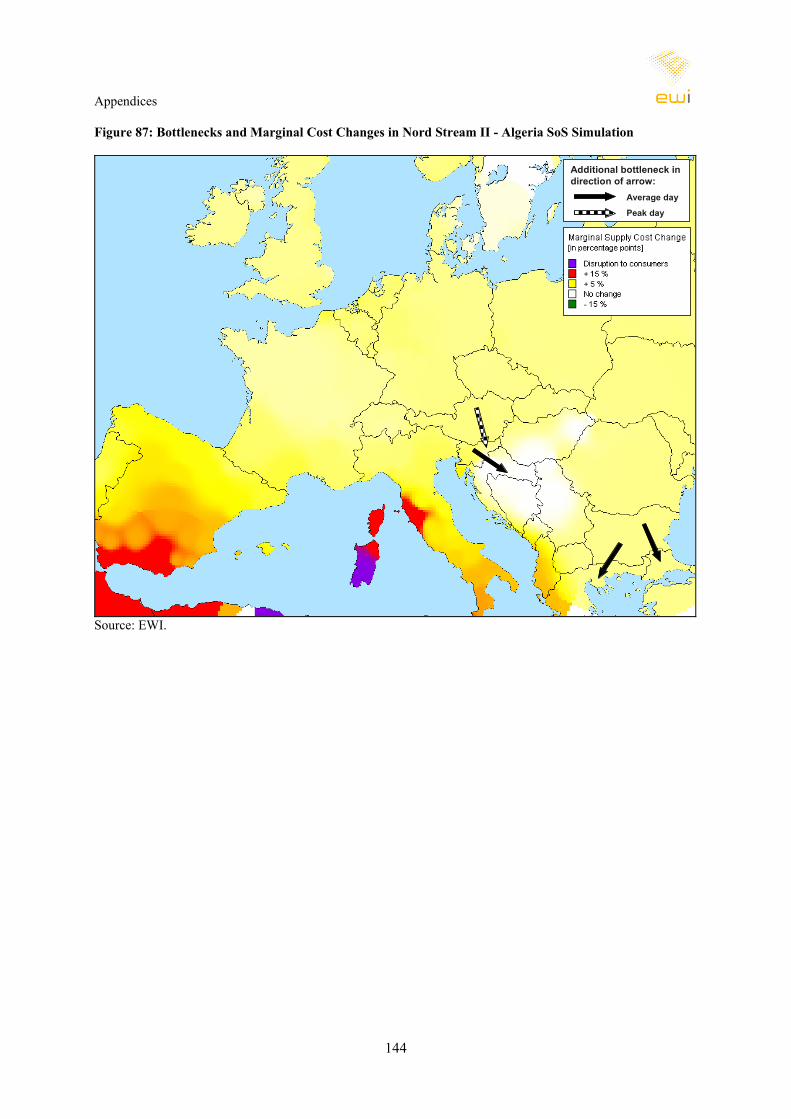
Appendices
144
Figure 87: Bottlenecks and Marginal Cost Changes in Nord Stream II - Algeria SoS Simulation
Additional bottleneck in direction of arrow:
Average day
Peak day
Source: EWI.
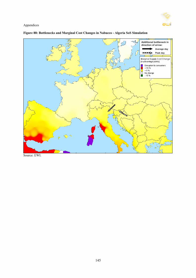
Appendices
145
Figure 88: Bottlenecks and Marginal Cost Changes in Nabucco - Algeria SoS Simulation
Additional bottleneck in direction of arrow:
Average day
Peak day
Source: EWI.

Appendices
146
Figure 89: Bottlenecks and Marginal Cost Changes in DG TREN - Algeria SoS Simulation
Additional bottleneck in direction of arrow:
Average day
Peak day
Source: EWI.

Appendices
147
Appendix E: Short description of MAGELAN Gas Supply Model MAGELAN is a long-term optimisation model of investments in natural gas production and
transport. It was developed at EWI (Seeliger, 2006) to optimise natural gas supply including
investments in production and infrastructure capacity up to 2035. It is an intertemporal and
interregional cost-minimisation model. The model's objective function includes both capital
and operating costs of global gas production and transport. Inefficiency, which could arise due
to strategic behaviour by market players, is therefore not reproduced by the model. (However,
incorporating such strategic actions would require strong assumptions regarding the type of
competition which in turn would significantly impact the results of the model.) Using linear
optimisation as an approach yields the advantage that results are solely based on objective
data. These results can therefore be interpreted as a first-best benchmark in the sense that they
represent the social welfare maximising outcome.
The optimisation in MAGELAN is subject to all relevant technical restrictions in production
and transportation of natural gas. That includes limited reserves and resources, the need to
balance demand and supply as well as in- and outflows for each country (and the system as
whole) and all capacity restrictions for infrastructure.79 The gas world in MAGELAN is
modelled as an interconnected grid consisting of 139 nodes for production, transport and
consumption. One node usually represents one country. In countries where production or
liquefaction or regasification of LNG takes or might in the future take place, additional nodes
have been implemented to provide for these facilities. A map of the coverage of the model
which includes all potential pipeline and LNG connections is depicted in Figure 90.
Major inputs of the model are assumptions on demand developments, existing reserves and
production costs per production region as well as existing infrastructure and all relevant cost
parameters. Based on existing capacities of the transport and production stages, the model can
in later periods endogenously expand capacities or build new facilities where possible (as
illustrated in Figure 90). Further, optimal production and transported volumes between nodes
are determined endogenously. Model outputs are therefore all capacity additions and
expansions as well as production per production region and volume flows between nodes on
an annual level.
79 A mathematical formulation of the model can be found in Seeliger (2006).
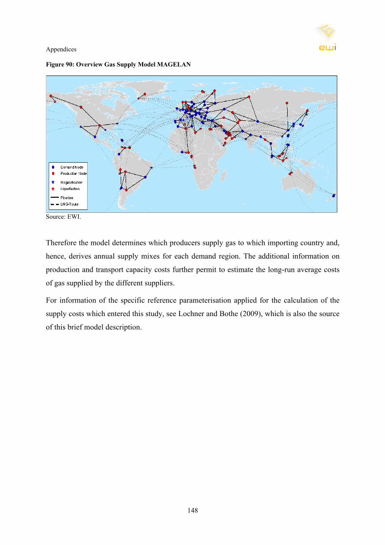
Appendices
148
Figure 90: Overview Gas Supply Model MAGELAN
Source: EWI.
Therefore the model determines which producers supply gas to which importing country and,
hence, derives annual supply mixes for each demand region. The additional information on
production and transport capacity costs further permit to estimate the long-run average costs
of gas supplied by the different suppliers.
For information of the specific reference parameterisation applied for the calculation of the
supply costs which entered this study, see Lochner and Bothe (2009), which is also the source
of this brief model description.