Model 707702 Computation Function Setup Software User's Manual

User'sManual

IM 707702-61E2nd Edition

Model 707702Computation Function SetupSoftware

1IM 707702-61E

ForewordThank you for purchasing the Computation Function Setup Software (Model: 707702).

This User’s Manual contains useful information about the operations and functions of the

software.

To ensure correct use, please read this manual thoroughly before operating the

software. Keep this manual in a safe place for quick reference in the event a question

arises.

The computation functions provided by this software serve to extend the capabilities of

the WE7000 Control Software’s Waveform Monitor or Viewer. The functions and

operating procedures of the WE7000 Control Software are described in the User’s

Manual listed below.

Manual Title Manual No. Description

WE7000 User’s Manual IM707001-01E Included with the Measuring Station WE800/WE400

This package contains the following items:

• Computation Function Setup Software (Model: 707702) setup disk: 1 floppy disk

• User’s Manual IM707702-61E (this manual): 1 piece

Notes• The WE7000 Control Software (Ver. 4.0.3.0 or later) must be installed on the PC in

order to use the Computation Function Setup Software (Model: 707702)

• The contents of this manual describe Version 1.03 of the Computation Function

Setup Software (Model: 707702). If you are using another version of the software,

the operating procedures and/or figures given in this manual may differ from those

corresponding to your version of the software.

• The contents of this manual are subject to change without prior notice as a result of

continuing improvements to the instrument’s performance and functions.

• Every effort has been made in the preparation of this manual to ensure the accuracy

of its contents. However, should you have any questions or find any errors, please

contact your nearest YOKOGAWA dealer as listed on the back cover of this manual.

• Copying or reproducing all or any part of the contents of this manual without

YOKOGAWA’s permission is strictly prohibited.

Trademarks• Microsoft, Windows, and Windows NT are either registered trademarks or trademarks

of Microsoft Corporation in the United States and/or other countries.

• Adobe and Acrobat are trademarks of Adobe Systems Incorporated.

• All other company and product names used in this manual are trademarks or

registered trademarks of their respective companies.

Revisions1st edition: February 2000

2nd edition: January 2001

Disk No. WE13

2nd Edition: January 2001 (YK)

All Rights Reserved, Copyright © 2000 Yokogawa Electric Corporation

2 IM 707702-61E

Notes on Using This Product

Storing and Backing Up the Setup DiskPlease store the original setup disk (floppy disk) in a safe place. Back up the contents of

the setup disk to another floppy disk (2HD: 1.44 MB). Use the backup copy for all future

operations including installation to the hard disk.

AgreementRestriction on Use

Use of this software by more than one computer at the same time is prohibited. Use by

more than one user is also prohibited.

Transfer and Lending

Transfer or lending of this product to any third party is prohibited.

Guarantee

Should a physical deficiency be found on the original setup disk or this manual upon

opening the product package, please promptly inform Yokogawa. The claim must be

made within seven days from the date you received the product in order to receive a

replacement free of charge.

Exemption from Responsibility

Yokogawa Electric Corporation provides no guarantees other than for physical

deficiencies found on the original setup disk or this manual upon opening the product

package. Yokogawa Electric Corporation shall not be held responsible by any party for

any losses or damage, direct or indirect, caused by the use or any unpredictable defect

of the product.

Conventions Used in this ManualUnit

k: Denotes 1000. Example: 100 kHz

K: Denotes 1024. Example 720 KB

Displayed Characters

Alphanumeric characters enclosed with [ ] usually refer to characters or setting values

that are displayed on the screen.

Symbols

Note Provides important information for the proper operation of the software.

3IM 707702-61E

PC System Requirements

HardwarePC

PC on which Windows 95/98/Me, Windows NT4.0, Windows 2000 Pro runs.

CPU: Pentium 133 MHz or higher

Internal Memory

48 MB or more (64 MB or more recommended)

Hard Disk

Free space of at least 20 MB.

Drive

One 3.5-inch floppy disk drive. The disk drive is used to install the software.

Display

Display supported by Windows95/98/Me, Windows NT4.0, or Windows 2000 Pro with a

resolution of 800×600 or better. Analog RGB with 65,536 colors or more recommended.

Operating SystemMicrosoft Windows 95/98/Me, Windows NT4.0, Windows 2000 Pro.

4 IM 707702-61E

5IM 707702-61E

1

2

3

Index

Contents

Foreword ................................................................................................................................................. 1

Notes on Using This Product ................................................................................................................... 2

PC System Requirements ....................................................................................................................... 3

Setting Up the Computation Function in the WE7000 Control Software ................................................. 6

Checking the Computation Function Setup ............................................................................................. 7

Chapter 1 Explanation of Functions1.1 Overview of Functions ............................................................................................................... 1-1

1.2 Details of Various Computations ............................................................................................... 1-4

Chapter 2 Operating Procedures2.1 User-defined Computation ........................................................................................................ 2-1

2.2 Averaging .................................................................................................................................. 2-4

2.3 Automated Measurement of Waveform Parameters ................................................................. 2-5

2.4 Displaying the Computation Results ......................................................................................... 2-7

2.5 Saving the Computation Results ............................................................................................... 2-8

Chapter 3 SpecificationsSpecifications ....................................................................................................................................... 3-1

Index .............................................................................................................................................................. Index-1

6 IM 707702-61E

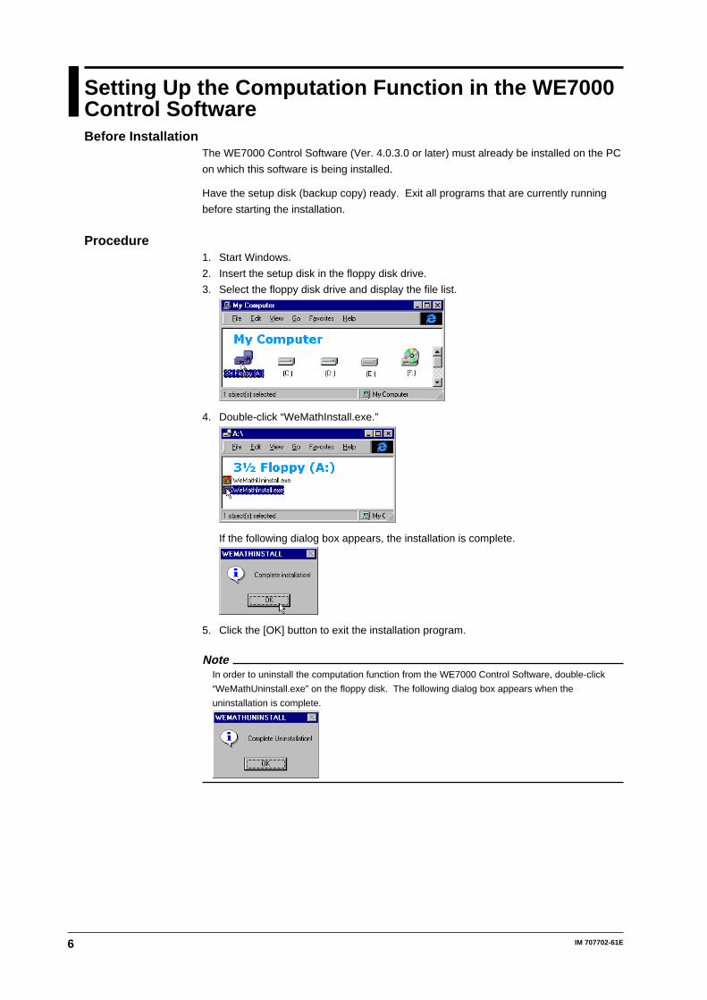
Setting Up the Computation Function in the WE7000Control SoftwareBefore Installation

The WE7000 Control Software (Ver. 4.0.3.0 or later) must already be installed on the PC

on which this software is being installed.

Have the setup disk (backup copy) ready. Exit all programs that are currently running

before starting the installation.

Procedure1. Start Windows.

2. Insert the setup disk in the floppy disk drive.

3. Select the floppy disk drive and display the file list.

4. Double-click “WeMathInstall.exe.”

If the following dialog box appears, the installation is complete.

5. Click the [OK] button to exit the installation program.

NoteIn order to uninstall the computation function from the WE7000 Control Software, double-click

“WeMathUninstall.exe” on the floppy disk. The following dialog box appears when the

uninstallation is complete.

7IM 707702-61E

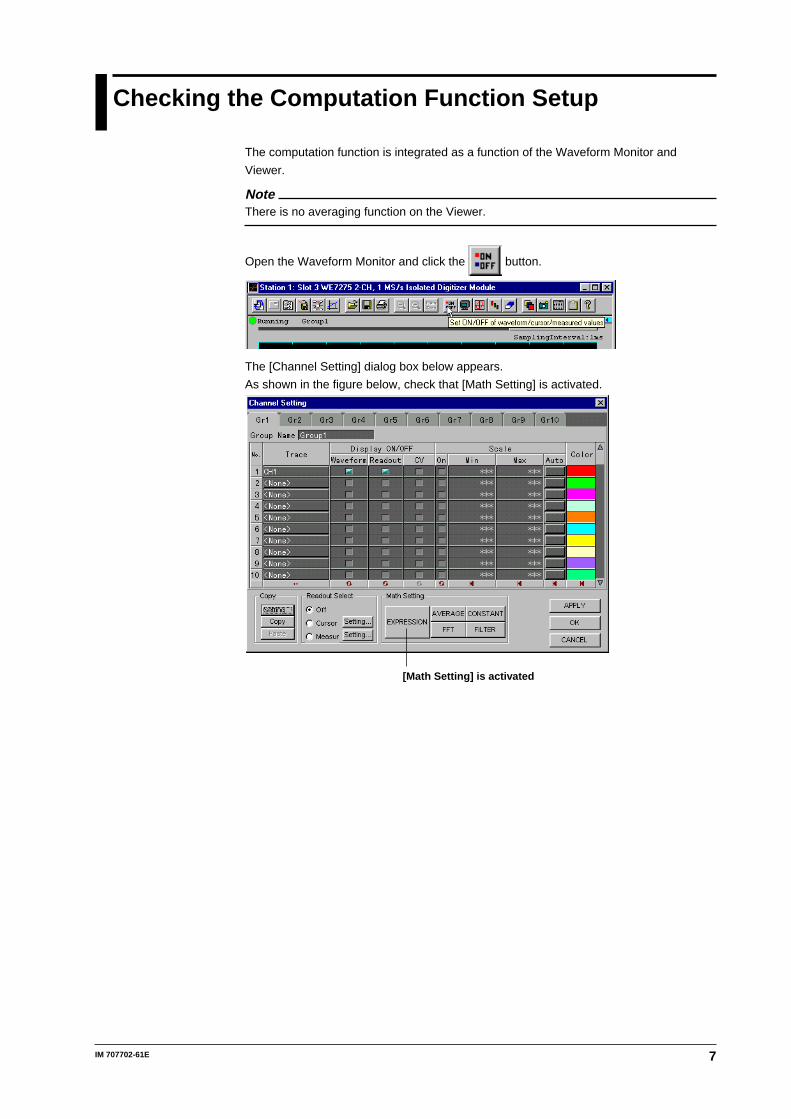
Checking the Computation Function Setup

The computation function is integrated as a function of the Waveform Monitor and

Viewer.

NoteThere is no averaging function on the Viewer.

Open the Waveform Monitor and click the button.

The [Channel Setting] dialog box below appears.

As shown in the figure below, check that [Math Setting] is activated.

[Math Setting] is activated

1-1IM 707702-61E

Exp

lanatio

n o

f Fu

nctio

ns

11.1 Overview of Functions

User-defined ComputationThe following variables and operators can be combined to create an equation. The

resulting computed waveform can then be displayed.

Variables

Variable Example Description

Cx C1+C2 The measured value of the specified channel, CHx.Mx ABS(M1) Computed (Math) value.T SIN(T) The accumulated value of the number of data points on

the time axis.

X: Number

Operators

If the acquisition mode is set to Free Run, the computed waveform that uses the

operators in the table below starting with BIN cannot be displayed while the

measurement is in progress. A and B represent the Upper and Lower threshold levels,

respectively.

Operator Example Description

+, - , *, / C1+C2 Four arithmetical operations of the two specifiedwaveforms

ABS ABS(M1) The absolute value of the specified waveformSQRT SQRT(C2) The square root of the specified waveformLOG LOG(C1) The logarithm of the specified waveformEXP EXP(C1) The exponent of the specified waveformSIN SIN(T) The sine of the specified waveformCOS COS(C1) The cosine of the specified waveformTAN TAN(C1) The tangent of the specified waveformATAN ATAN(C1, C2) The arc tangent of the two specified waveforms (a value

within ±π)P2 P2(C1) The square of the specified waveformP3 P3(C1) The cube of the specified waveformF1 F1(C1, C2) C12+C22

of the specified waveformsF2 F2(C1, C2) C12–C22 of the specified waveformsK1-10 C1+K1 Constants (assign an arbitrary value)BIN BIN(C1, A, B) The binary conversion of the specified waveformPWHH PWHH(M1, A, B) Pulse width computation from the rising edge to the next

rising edge.PWHL PWHL(C2, A, B) Pulse width computation from the rising edge to the next

falling edge.PWLH PWLH(C1, A, B) Pulse width computation from the falling edge to the next

rising edge.PWLL PWLL(C1, A, B) Pulse width computation from the falling edge to the next

falling edge.PWXX PWXX(C2, A, B) Pulse width computation from the rising or falling edge to

the next rising or falling edgeMEAN MEAN(C1) The 10th order moving average of the specified waveformDIF DIF(C1) The derivative of the specified waveformDDIF DDIF(C1) The second order derivative of the specified waveformINTG INTG(C1) The integration of the specified waveformIINTG IINTG(C1) The secondary integration of the specified waveformPH PH(C1, C2) The phase difference between the two specified

waveformsHLBT HLBT(C1) The Hilbert transform of the specified waveformFILT1 FILT1(C1) Apply a filter to the specified waveformFILT2 FILT2(C1) Apply a filter to the specified waveformLS-REAL LS-REAL(C1) The real part of the specified waveform’s linear spectrumLS-IMAG LS-IMAG(C1) The imaginary part of the specified waveform’s linear

spectrumLS-MAG LS-MAG(C1) The amplitude of the specified waveform’s linear spectrumLS-LOGMAG LS-LOGMAG(C1) The logarithmic amplitude of the specified waveform’s

linear spectrumLS-PHASE LS-PHASE(C1) The phase of the specified waveform’s linear spectrumRS-RS-MAG RS-MAG(C1) The amplitude of the specified waveform’s rms spectrum

Chapter 1 Explanation of Functions

1-2 IM 707702-61E

Operator Example Description

RS-LOGMAG RS-LOGMAG(C1) The logarithmic amplitude of the specified waveform’s rmsspectrum

PS-MAG PS-MAG(C1) The amplitude of the specified waveform’s powerspectrum

PS-LOGMAG PS-LOGMAG(C1) The logarithmic amplitude of the specified waveform’spower spectrum

PSD-MAG PSD-MAG(C1) The amplitude of the specified waveform’s powerspectrum density

PSD-LOGMAG PSD-LOGMAG(C1) The logarithmic amplitude of the specified waveform’spower spectrum density

CS-REAL CS-REAL(C1, C2) The real part of the cross spectrum of the two specifiedwaveforms

CS-IMAG CS-IMAG(C1, C2) The imaginary part of the cross spectrum of the twospecified waveforms

CS-MAG CS-MAG(C1, C2) The amplitude of the cross spectrum of the two specifiedwaveforms

CS-LOGMAG CS-LOGMAG(C1, C2) The logarithmic amplitude of the cross spectrum of the twospecified waveforms

CS-PHASE CS-PHASE(C1, C2) The phase of the cross spectrum of the two specifiedwaveforms

TF-REAL TF-REAL(C1, C2) The real part of the transfer function of the two specifiedwaveforms

TF-IMAG TF-IMAG(C1, C2) The imaginary part of the transfer function of the twospecified waveforms

TF-MAG TF-MAG(C1, C2) The amplitude of the transfer function of the two specifiedwaveforms

TF-LOGMAG TF-LOGMAG(C1, C2) The logarithmic amplitude of the transfer function of thetwo specified waveforms

TF-PHASE TF-PHASE(C1, C2) The phase of the transfer function of the two specifiedwaveforms

CH-MAG CH-MAG(C1, C2) The amplitude of the coherence function of the twospecified waveforms

AveragingThe measured waveform (before computation) and computed waveform are averaged

(linearly averaged/exponentially averaged) or their peaks are computed. The resultant

waveform is displayed. However, this is possible only when the acquisition mode is set

to some mode other than free run and memory partition is disabled.

NoteThere is no averaging function on the Viewer.

Linear Averaging

The specified number (averaging block length) of values are linearly summed and then

divided by the number of points summed. The averaging block length can be in the

range from 2 to 65536. The resultant waveform is displayed.

AN=N

N

n=1Σ Xn

XnN

: nth measured value: averaging block length

Exponential Averaging

The average is determined by attenuating the effects of past data according to the

specified attenuation constant (2 to 256, in 2n steps). The resultant waveform is

displayed.


1-3IM 707702-61E

Exp

lanatio

n o

f Fu

nctio

ns

1An= {(N–1)An–1+Xn}

1N

AnXnN

: nth averaged value: nth measured value: Attenuation constant

Peak Hold

The maximum value, among data located at the same time/frequency axis position of the

waveform being updated using triggers or other events, is determined. The resultant

waveform is displayed. For every computation, the new value is compared to the past

value and the larger one is displayed.

Saving the Computed Waveform DataLike the measured waveform, the user-defined computation waveform, average

waveform, and peak-held waveform can be saved to a file.

Automated Measurement of Waveform ParametersThe twenty types of waveform parameter measurements (see page 2-6), that were

previously only possible on the digital oscilloscope, can now, with the addition of this

software, be performed on data from other modules. In addition, the range over which

the waveform parameters are measured can be specified using cursors. The

measurement results can be saved to a file.


1-4 IM 707702-61E

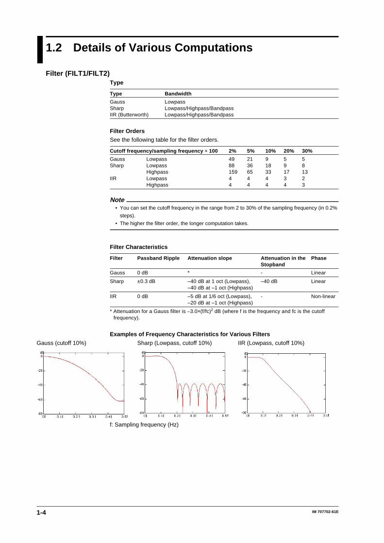
1.2 Details of Various Computations

Filter (FILT1/FILT2)Type

Type Bandwidth

Gauss LowpassSharp Lowpass/Highpass/BandpassIIR (Butterworth) Lowpass/Highpass/Bandpass

Filter Orders

See the following table for the filter orders.

Cutoff frequency/sampling frequency × 100 2% 5% 10% 20% 30%

Gauss Lowpass 49 21 9 5 5Sharp Lowpass 88 36 18 9 8

Highpass 159 65 33 17 13IIR Lowpass 4 4 4 3 2

Highpass 4 4 4 4 3

Note• You can set the cutoff frequency in the range from 2 to 30% of the sampling frequency (in 0.2%

steps).

• The higher the filter order, the longer computation takes.

Filter Characteristics

Filter Passband Ripple Attenuation slope Attenuation in the PhaseStopband

Gauss 0 dB * - Linear

Sharp ±0.3 dB –40 dB at 1 oct (Lowpass), –40 dB Linear–40 dB at –1 oct (Highpass)

IIR 0 dB –5 dB at 1/6 oct (Lowpass), - Non-linear–20 dB at –1 oct (Highpass)

* Attenuation for a Gauss filter is –3.0×(f/fc)2 dB (where f is the frequency and fc is the cutofffrequency).

Examples of Frequency Characteristics for Various Filters

Gauss (cutoff 10%) Sharp (Lowpass, cutoff 10%) IIR (Lowpass, cutoff 10%)

f: Sampling frequency (Hz)

1-5IM 707702-61E

Exp

lanatio

n o

f Fu

nctio

ns

1Hilbert Function (HLBT)

Normally, when we analyze a real time signal, it is convenient to think of the signal as the

real part of a complex valued signal. Analysis is often more convenient when done using

the complex signal. Given that the real time signal is considered to be the real part of

the complex signal, the imaginary part is then equal to the Hilbert transform of the real

part. When performing a Hilbert transform on a signal in the time domain, the signal is

first transformed into the frequency domain using the Fourier transform. Next, the phase

of each frequency component is shifted by -90 degrees if the frequency is positive and

+90 degrees if negative. Lastly, the Hilbert transform is completed by taking the inverse

Fourier transform. As can be seen from the above description, the Hilbert transform

does not change the order of the individual variables. The Hilbert transform of a time

signal results in another time signal.

Application Example

The Hilbert transform can be used to analyze an envelope waveform.

AM (amplitude modulation): SQRT(C1*C1+HLBT(C1)*HLBT(C1))

Demodulation of a FM signal: DIF(PH(C1, HLBT(C1)))

Phase Function (PH)Phase function PH(C1, C2) computes tan-1 (C1/C2). However, the phase function takes

the phase of the previous point into consideration and continues to sum even when the

value exceeds ±π (The ATAN function reflects at ±π). The unit is radians.

Previous point

Previous point

θ2

θ2

θ2=θ1+∆θ2 θ2=θ1–∆θ2

∆θ2

∆θ2

θ1

θ1

Binary Conversion (BIN)Performs binary conversion with respect to the specified threshold level.

The threshold level is specified as follows:

A and B represent the Upper and Lower threshold levels, respectively.

BIN(C1, A, B)

1

0

Upper threshold level

Lower threshold level


1-6 IM 707702-61E


Pulse Width Computation (PWHH/PWHL/PWLH/PWLL/PWXX)The signal is converted into binary values by comparing to a preset threshold level, and

the time of the pulse width is plotted as the Y-axis value for that interval.

The following 4 intervals are available:

PWHH: From the rising edge to the next rising edge.

PWHL: From the rising edge to the next falling edge.

PWLH: From the falling edge to the next rising edge.

PWLL: From the falling edge to the next falling edge.

PWXX: From the rising or falling edge to the next rising or falling edge.

The threshold level is specified as follows:

A and B represent the Upper and Lower threshold levels, respectively.

PWHH (C1, A, B)

When the Interval is Set to PWHH

Waveform to be computed

A: Upper threshold level

t1 t2 t3

Computed waveform

B: Lower threshold level

t1

t2 t3

FFTLinear Spectrum (LS-REAL/LS-IMAG/LS-MAG/LS-LOGMAG/LS-PHASE)

The linear spectrum is directly determined by the FFT. The power spectrum and cross

spectrum can be determined from one or two linear spectra.

The FFT is a complex function, and thus the linear spectrum is composed of both a real

and an imaginary part. The magnitude and phase of the frequency components of the

measured waveform can be derived from the real and imaginary parts of the FFT result.

The following spectra can be determined:

Item Expression Computation

Real part LS-REAL RImaginary part LS-IMAG IMagnitude LS-MAG (R2+I2)Log magnitude LS-LOGMAG 20×log (R2+I2)Phase LS-PHASE tan–1(I/R)

Log magnitude reference (0 dB): 1 VpeakR, I: R and I represent the real part and the imaginary part, respectively, when each frequencycomponent G of a linear spectrum is represented by “R+jI.”

Rms Value Spectrum (RS-RS-MAG/RS-LOGMAG)

Rms value spectrum expresses the rms value of the magnitude of the linear spectrum. It

does not contain phase information.



Magnitude RS-MAG (R2+I2)/2Log magnitude RS-LOGMAG 20×log (R2+I2)/2

Log magnitude reference (0 dB): 1 Vrms

1-7IM 707702-61E

Exp

lanatio

n o

f Fu

nctio

ns

1


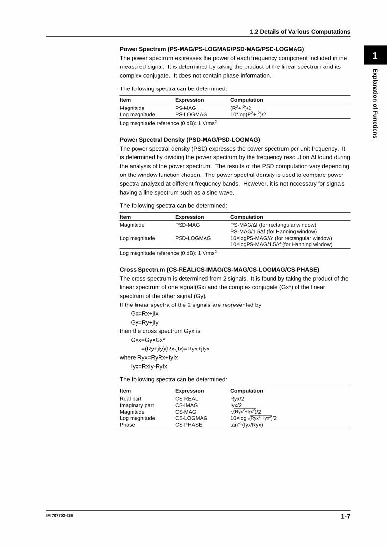
Power Spectrum (PS-MAG/PS-LOGMAG/PSD-MAG/PSD-LOGMAG)

The power spectrum expresses the power of each frequency component included in the

measured signal. It is determined by taking the product of the linear spectrum and its

complex conjugate. It does not contain phase information.



Magnitude PS-MAG (R2+I2)/2Log magnitude PS-LOGMAG 10*log(R2+I2)/2

Log magnitude reference (0 dB): 1 Vrms2

Power Spectral Density (PSD-MAG/PSD-LOGMAG)

The power spectral density (PSD) expresses the power spectrum per unit frequency. It

is determined by dividing the power spectrum by the frequency resolution ∆f found during

the analysis of the power spectrum. The results of the PSD computation vary depending

on the window function chosen. The power spectral density is used to compare power

spectra analyzed at different frequency bands. However, it is not necessary for signals

having a line spectrum such as a sine wave.



Magnitude PSD-MAG PS-MAG/∆f (for rectangular window)PS-MAG/1.5∆f (for Hanning window)

Log magnitude PSD-LOGMAG 10×logPS-MAG/∆f (for rectangular window)10×logPS-MAG/1.5∆f (for Hanning window)

Log magnitude reference (0 dB): 1 Vrms2

Cross Spectrum (CS-REAL/CS-IMAG/CS-MAG/CS-LOGMAG/CS-PHASE)

The cross spectrum is determined from 2 signals. It is found by taking the product of the

linear spectrum of one signal(Gx) and the complex conjugate (Gx*) of the linear

spectrum of the other signal (Gy).

If the linear spectra of the 2 signals are represented by

Gx=Rx+jIx

Gy=Ry+jIy

then the cross spectrum Gyx is

Gyx=Gy×Gx*

=(Ry+jIy)(Rx-jIx)=Ryx+jIyx

where Ryx=RyRx+IyIx

Iyx=RxIy-RyIx



Real part CS-REAL Ryx/2Imaginary part CS-IMAG Iyx/2Magnitude CS-MAG (Ryx2+Iyx2)/2Log magnitude CS-LOGMAG 10×log (Ryx2+Iyx2)/2Phase CS-PHASE tan–1(Iyx/Ryx)

1-8 IM 707702-61E

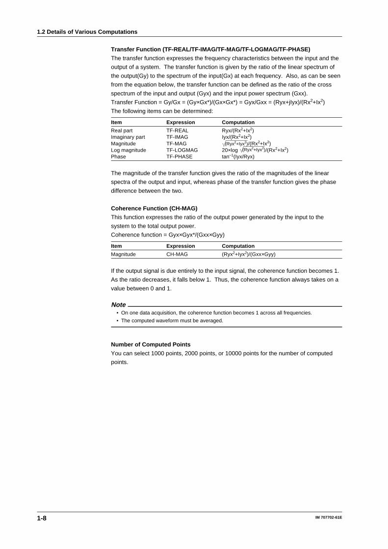
Transfer Function (TF-REAL/TF-IMAG/TF-MAG/TF-LOGMAG/TF-PHASE)

The transfer function expresses the frequency characteristics between the input and the

output of a system. The transfer function is given by the ratio of the linear spectrum of

the output(Gy) to the spectrum of the input(Gx) at each frequency. Also, as can be seen

from the equation below, the transfer function can be defined as the ratio of the cross

spectrum of the input and output (Gyx) and the input power spectrum (Gxx).

Transfer Function = Gy/Gx = (Gy×Gx*)/(Gx×Gx*) = Gyx/Gxx = (Ryx+jIyx)/(Rx2+Ix2)

The following items can be determined:


Real part TF-REAL Ryx/(Rx2+Ix2)Imaginary part TF-IMAG Iyx/(Rx2+Ix2)Magnitude TF-MAG (Ryx2+Iyx2)/(Rx2+Ix2)Log magnitude TF-LOGMAG 20×log (Ryx2+Iyx2)/(Rx2+Ix2)Phase TF-PHASE tan–1(Iyx/Ryx)

The magnitude of the transfer function gives the ratio of the magnitudes of the linear

spectra of the output and input, whereas phase of the transfer function gives the phase

difference between the two.

Coherence Function (CH-MAG)

This function expresses the ratio of the output power generated by the input to the

system to the total output power.

Coherence function = Gyx×Gyx*/(Gxx×Gyy)


Magnitude CH-MAG (Ryx2+Iyx2)/(Gxx×Gyy)

If the output signal is due entirely to the input signal, the coherence function becomes 1.

As the ratio decreases, it falls below 1. Thus, the coherence function always takes on a

value between 0 and 1.

Note• On one data acquisition, the coherence function becomes 1 across all frequencies.

• The computed waveform must be averaged.

Number of Computed Points

You can select 1000 points, 2000 points, or 10000 points for the number of computed

points.


1-9IM 707702-61E

Exp

lanatio

n o

f Fu

nctio

ns

1


About Time Windows

You can select rectangular, Hanning, or flattop as the time window.

The rectangular window is best suited to transient signals, such as an impulse wave, that

attenuate completely within the time window. The Hanning window allows continuity of

the signal by gradually attenuating the parts of the signal located near the ends of the

time window down to the “0” level. Hence, it is best suited to continuous signals. The

frequency resolution of the Hanning window is higher compared with the Flattop window.

However, the flattop window has a higher level of accuracy of the spectrum. When the

waveform being analyzed is a continuous signal, consider the above characteristics

when selecting the proper window to use.

T

T

T

T

t

Sine wave

Window Integral Power spectrumRectangular

window

Hanning window

Rectangular window

Hanning window

Flattop window

: W(t)=u(t)–u(t–T) U(t) : Step function

: W(t)=0.5–0.5cos(2π )

: W(t)={0.54–0.46cos(2π )}

T

TFlattop window

tT

tT

sin{2π(1–2t/T)}2π(1–2t/T)

2-1IM 707702-61E

Op

erating

Pro

cedu

res

2

2.1 User-defined Computation

Procedure1. Click the [EXPRESSION] button of the [Channel Setting] dialog box.

[Expression] button2. In the [Math Expression] dialog box below, set the expression, label, unit, and the

ON/OFF condition of the averaging of the computed waveform.

Up to 10 expressions can be specified.

If you select multiple [Math] buttons by dragging the mouse (the characters of the

selected button turn red) and click the copy & paste button, the first [Math] setting is

copied to the other [Math] settings. If you click the Average all ON/OFF button, the

averaging function of the selected [Math] settings are turn ON/OFF at once.

Averaging allON/OFF button

Label entry box (up to 31 characters)Unit entry box (up to 15 characters)

Expression setting boxComputed waveform averagingON/OFF button

When selectingor deselecting all[Math] settings

[Math] button

Copy & paste buttonClick the expression setting box to display the following dialog box.

Displays other equations

Label entry box(up to 31 characters)

Display the operatorselection menu

Unit entry box(up to 15 characters)

Buttons used to entervalues and variables

Expression entry box

Displaying the Operator Selection Menu

Chapter 2 Operating Procedures

2-2 IM 707702-61E

In the menu, the operators are classified into the following groups:Basic: ABS, SQRT, LOG, EXP, P2, P3, F1, F2Trigonometric: SIN, COS, TAN, ATAN, PHPulse Width: PWHH, PWHL, PWLH, PWLL, PWXXDIF & INTG: DIF, DDIF, INTG, IINTGFilter: FILT1, FILT2, HLBT, MEAN, BINFFT > LS: LS-REAL, LS-IMAG, LS-MAG, LS-LOGMAG, LS-PHASE

RS: RS-MAG, RS-LOGMAGPS: PS-MAG, PS-LOGMAG, PSD-MAG, PSD-LOGMAGCS: CS-REAL, CS-IMAG, CS-MAG, CS-LOGMAG, CS-PHASETF: TF-REAL, TF-IMAG, TF-MAG, TF-LOGMAG, TF-PHASECH: CH-MAG

Setting the Constants K1 through K10

1. Click the [CONSTANT] button of the [Channel Setting] dialog box.

[CONSTANT] button

2. Set the necessary constants, K1 through K10, in the [Constant Setting] dialog box.

The numerical range allowed is -1.0000E+30 to 1.0000E+30.

Setting the Filters (FILT1/FILT2)

1. Click the [FILTER] button of the [Channel Setting] dialog box.

[FILTER] button

2. Set the [Type], [Band], and [CutOff1] in the [Filter Setting] dialog box.

Select the type and bandwidth from the following list of choices:

Gauss: Lowpass

Sharp: Lowpass/Highpass/Bandpass

IIR (Butterworth): Lowpass/Highpass/Bandpass

The cutoff frequency is specified as a percentage of the sampling frequency. The

range is from 2.0% to 30.0% (0.2% resolution). If the bandwidth is set to [Bandpass],

specify both cutoff frequencies, [CutOff1] and [CutOff2].


2-3IM 707702-61E

Op

erating

Pro

cedu

res

2

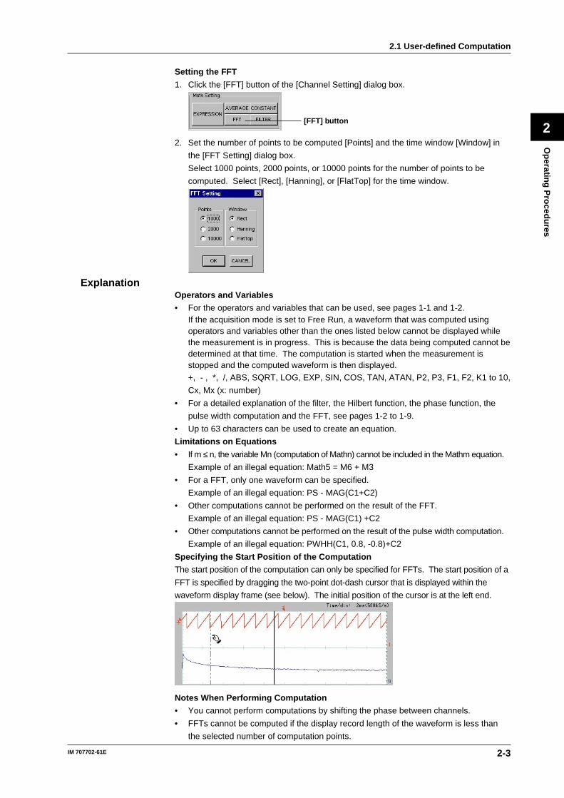
Setting the FFT

1. Click the [FFT] button of the [Channel Setting] dialog box.

[FFT] button

2. Set the number of points to be computed [Points] and the time window [Window] in

the [FFT Setting] dialog box.

Select 1000 points, 2000 points, or 10000 points for the number of points to be

computed. Select [Rect], [Hanning], or [FlatTop] for the time window.

ExplanationOperators and Variables

• For the operators and variables that can be used, see pages 1-1 and 1-2.If the acquisition mode is set to Free Run, a waveform that was computed usingoperators and variables other than the ones listed below cannot be displayed whilethe measurement is in progress. This is because the data being computed cannot bedetermined at that time. The computation is started when the measurement isstopped and the computed waveform is then displayed.

+, - , *, /, ABS, SQRT, LOG, EXP, SIN, COS, TAN, ATAN, P2, P3, F1, F2, K1 to 10,

Cx, Mx (x: number)

• For a detailed explanation of the filter, the Hilbert function, the phase function, the

pulse width computation and the FFT, see pages 1-2 to 1-9.

• Up to 63 characters can be used to create an equation.

Limitations on Equations

• If m ≤ n, the variable Mn (computation of Mathn) cannot be included in the Mathm equation.

Example of an illegal equation: Math5 = M6 + M3

• For a FFT, only one waveform can be specified.

Example of an illegal equation: PS - MAG(C1+C2)

• Other computations cannot be performed on the result of the FFT.

Example of an illegal equation: PS - MAG(C1) +C2

• Other computations cannot be performed on the result of the pulse width computation.

Example of an illegal equation: PWHH(C1, 0.8, -0.8)+C2

Specifying the Start Position of the Computation

The start position of the computation can only be specified for FFTs. The start position of a

FFT is specified by dragging the two-point dot-dash cursor that is displayed within the

waveform display frame (see below). The initial position of the cursor is at the left end.

Notes When Performing Computation

• You cannot perform computations by shifting the phase between channels.

• FFTs cannot be computed if the display record length of the waveform is less than

the selected number of computation points.


2-4 IM 707702-61E

2.2 Averaging

Procedure1. Click the [AVERAGE] button of the [Channel Setting] dialog box.

[AVERAGE] button

2. Select [Linear], exponential averaging [Exp.], or [Peak Hold] for the averaging

method in the [Average Setting] dialog box.

If [Linear] is selected, specify the average count in the range from 2 to 65536. In

linear averaging, the measurement is automatically stopped upon reaching the

specified average count regardless of whether the measured waveform or the

computed waveform is being averaged.

If exponential averaging [Exp.] is selected, specify the attenuation constant in the

range from 2 to 256 (in 2n steps).

Select the [Channel Average] check box when you wish to average the measured

waveform. In this case, if the measured waveform data of each channel (C1 and C2,

for example) are used as variables in an equation, the averaged values are used to

compute the equation.

Select the averaging method

Check when averaging the measured data

ExplanationFor details on the various averaging methods, see page 1-2.

Initializing the Averaging

Click the waveform clear button ( ) of the Waveform Monitor or Viewer to clear the

displayed waveform. The averaging will be restarted and a new waveform will be

displayed.

Precautions and Limitations on Averaging

• Time domain computations are averaged in the time domain.

• For FFTs, averaging is performed in the frequency domain.

• When a computation condition is changed, averaging is restarted using the new

condition. Thus, the waveform data displayed before the change will be cleared.

• If a computation condition is changed while averaging the computed waveform, all

the computed waveform data up to that point are cleared.

• If the measurement (waveform acquisition) is restarted, averaging is also restarted

and the new waveform is displayed.

• Averaging cannot be performed when the acquisition mode is set to free run or when

memory partition is enabled.

• Averaging cannot be performed on pulse width computation waveforms.

• There is no averaging function on the Viewer.

2-5IM 707702-61E

Op

erating

Pro

cedu

res

2

2.3 Automated Measurement of WaveformParameters

Procedure1. Select [Measure] under the [Readout Select] option button of the [Channel Setting]

dialog box.

2. Click the [Setting] button located to the right of [Measure].

[Setting] button for [Measure]

[Measure] option button3. In the [Measure Item Setting] dialog box, check the boxes corresponding to the

waveform parameters to be measured.

To check all waveform parameters, click the [ALL ON] button. To remove all checks,

click the [ALL OFF] button.

ExplanationWaveform Parameters• Voltage-axis parameters

P-P Value

Max

Min

High Level

Low Level

Maximum: Maximum voltage [V] Average: Average voltage (1/n )Σxi [V]Minimum: Minimum voltage [V] RMS: rms value (1/ n )(Σ(xi)2)1/2 [V]High level: High level voltage [V] Middle: Center value of the amplitude (Max+Min)/2 [V]Low level: Low level voltage [V] Standard deviation: Standard deviation (1/n(Σx2–(Σx2)/n))1/2

Peak to peak value: P-P value (Max - Min) [V] Overshoot: (Max–High)/(High–Low)×100 [%]Amplitude: (High - Low) [V] Undershoot: (Low–Min)/(High–Low)×100 [%]

Overshoot

Undershoot

• Time-axis parameters

+Width -WidthPeriod

Distal line (90%)

Mesial line (50%)

Proximal line (10%)

Rise Time Fall Time

High Level (100%)

Low Level (0%)

Rise time: Rise time [s] +Duty: Duty cycle Width1/Period×100 [%]Fall time: Fall time [s] - Duty: Duty cycle Width2/Period×100 [%]Frequency: Frequency [Hz] + Width: Time width above the mesial value [s]Period : Period [s] - Width: Time width below the mesial value [s]

2-6 IM 707702-61E

2.3 Automated Measurement of Waveform Parameters

The high level is defined to be the highest amplitude level (100% level) within the

measurement range based on the frequency of voltage levels of the waveform while

taking into account the effects of ringing, spikes, and other phenomena. Low is the

lowest amplitude level (0% level). With these levels as references, the distal, mesial,

and proximal values are defined to be the 90%, 50%, and 10% levels, respectively.

Limitations When Performing Automated Measurement of Waveform Parameters

• Automated measurement of waveform parameters cannot be performed on snapshot

waveforms and accumulated waveforms.

• If the [Measure] box is checked in the operation panel of the Digital Oscilloscope

Module WE7111, automated measurement of waveform parameters is performed on

the module. However, the results of this computation function are displayed in place

of the results from the module. (The computed results of this computation function

have precedence over the results obtained on the module.) Therefore, remove the

check from the [Measure] box.

Specifying the Range for Automated Measurement of Waveform Parameters

You can specify the range over which the automated measurement of waveform

parameters is performed. As in the following figure, the range is specified by dragging

the two cursors (solid and dotted lines) displayed within the waveform display frame.

Saving the Results of the Automated Measurement of Waveform Parameters

When the automated measurement of waveform parameters is performed, up to 1000

points of the measured data are saved. The data are cleared when the measurement

range is changed, the measurement item is changed, or the measurement is restarted.

For details related to saving the data, see page 2-11.

2-7IM 707702-61E

Op

erating

Pro

cedu

res

2

2.4 Displaying the Computation Results

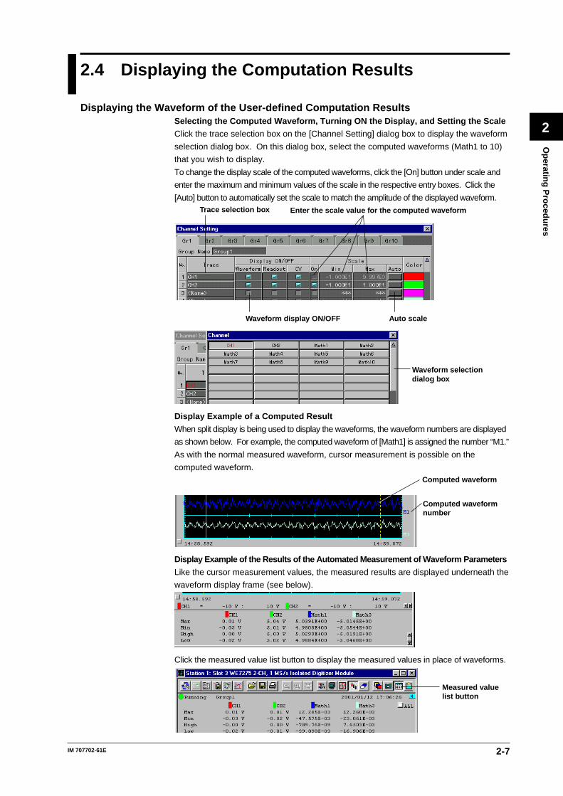
Displaying the Waveform of the User-defined Computation ResultsSelecting the Computed Waveform, Turning ON the Display, and Setting the Scale

Click the trace selection box on the [Channel Setting] dialog box to display the waveform

selection dialog box. On this dialog box, select the computed waveforms (Math1 to 10)

that you wish to display.

To change the display scale of the computed waveforms, click the [On] button under scale and

enter the maximum and minimum values of the scale in the respective entry boxes. Click the

[Auto] button to automatically set the scale to match the amplitude of the displayed waveform.Trace selection box Enter the scale value for the computed waveform

Waveform display ON/OFF Auto scale

Waveform selectiondialog box

Display Example of a Computed Result

When split display is being used to display the waveforms, the waveform numbers are displayed

as shown below. For example, the computed waveform of [Math1] is assigned the number “M1.”

As with the normal measured waveform, cursor measurement is possible on the

computed waveform.Computed waveform

Computed waveform number

Display Example of the Results of the Automated Measurement of Waveform Parameters

Like the cursor measurement values, the measured results are displayed underneath the

waveform display frame (see below).

Click the measured value list button to display the measured values in place of waveforms.

Measured valuelist button

2-8 IM 707702-61E

2.5 Saving the Computation Results

Procedure1. Click the data save button of the waveform viewer.

Data save button

Saving the Computed Waveform Data

2. The save dialog box opens (see figure below). Select the save format and name the

file. Select binary data (“*.wvf” extension), ASCII data in CSV format (“*.csv”

extension), or Excel link “*.” for the save format.

When the Save button is clicked when saving to CSV format, a dialog box appears

for you to select whether or not to include time axis information. Comments can be

saved to the file by entering text in the Comment box unless the file is saved in Excel

format. Select [Bitmap (*.bmp)] when you wish to save the displayed waveform as

image data in bitmap format. In this case, only one line of comment is saved as

image data.

Saving after Excel Linking

When [Excel (*.)] is selected, the displayed waveform data can be transferred directly

to Excel*. Clicking the [Save] button displays the dialog box shown below.

In this dialog box, enter the first cell to which to transfer the measured data in the

[Starting Cell] entry box and set whether or not to include time axis information using

the [Include Time Axis] check box. Set the starting cell to B3 or larger (B9 is default)

to allocate the minimum number of cells needed to transfer the data information.

Otherwise, an error will occur. All of the data information is transferred when you

select B9 as the starting cell.

To execute an Excel macro after transferring the data, check the [Execute Macro

After Linking] box and set the file name and macro name.

When you are ready, clicking the [OK] button starts Excel and the data are

transferred. Use the operations in Excel to manually save the data if you did not

specify a macro save operation.* Operation guaranteed on Microsoft Excel 97 only.

2-9IM 707702-61E

Op

erating

Pro

cedu

res

2


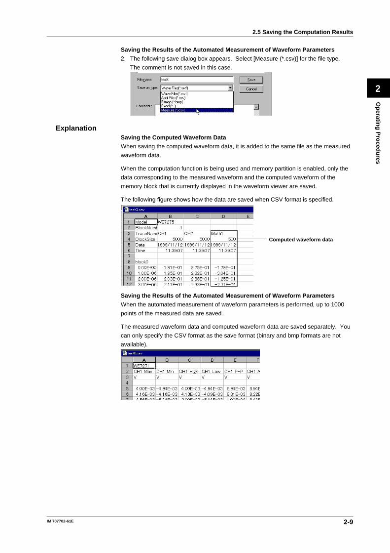
2. The following save dialog box appears. Select [Measure (*.csv)] for the file type.

The comment is not saved in this case.

ExplanationSaving the Computed Waveform Data

When saving the computed waveform data, it is added to the same file as the measured

waveform data.

When the computation function is being used and memory partition is enabled, only the

data corresponding to the measured waveform and the computed waveform of the

memory block that is currently displayed in the waveform viewer are saved.

The following figure shows how the data are saved when CSV format is specified.

Computed waveform data


When the automated measurement of waveform parameters is performed, up to 1000

points of the measured data are saved.

The measured waveform data and computed waveform data are saved separately. You

can only specify the CSV format as the save format (binary and bmp formats are not

available).

2.5 Saving the Computation Results

3-1IM 707702-61E

Sp

ecification

s

3

Specifications

User-defined ComputationNumber of Display Channels for Computed Waveforms

10

Waveforms on Which Computation Is to Be Performed

Measured waveforms and computed waveforms

Applicable Acquisition Modes

Trigger mode and free run mode (limitations on displaying the waveform while the

measurement is in progress)

Computation Accuracy

Single-precision floating point

Types of Computations

Operator types: four arithmetical operations, absolute value, square root, logarithm,

exponent, trigonometric functions, differentiation, integration, filter, Hilbert transform,

phase function, pulse width function, FFT, etc. (for details, see page 1-1)

Constants: Up to 10 constants can be specified

Number of characters that can be entered for creating equations: 63

Filter bandwidths: Select Low pass, high pass, or band pass.

Filter characteristics: Select Gaussian, sharp, or Butterworth

Number of points for taking the FFT: Select 1000, 2000, or 10000 points.

FFT window: Select rectangular, Hanning, or flattop.

Saving the computed waveform

Save as physical values to the same file as the measured waveform data.

AveragingData to Be Averaged

Measured data and computed data

Types

Linear averaging: Select the average count in the range from 2 to 65536.

Exponential averaging: Select the attenuation constant in the range from 2 to 256 (in 2n

steps).

Peak hold: Displays the maximum value among the data at the same time/frequency axis

position of the waveform.

Automated Measurement of Waveform ParametersMeasurement Parameters

Twenty parameters such as the maximum/minimum voltage, average voltage, rms value,

P-P value, overshoot, and undershoot (for details, see page 2-6).

Specifying the Measurement Range

Specify the measurement range using two cursors.

Saving the Measured Data

Up to 1000 points of measured data can be saved. The save format is CSV.

Chapter 3 Specifications

Index-1IM 707702-61E

Ind

ex

Index

Index

Index

Symbols

*.csv 2-8

*.wvf 2-8

A

ALL OFF 2-5

ALL ON 2-5

Auto 2-7

Automated Measurement of Waveform Parameters 1-3, 2-5

AVERAGE 1-2

Average Setting 2-4

B

Band 2-2

Bandpass 1-4, 2-2

Basic 2-2

BIN 1-5

Binary Conversion 1-5

Butterworth 1-4, 2-2

C

CH 2-2

CH-MAG 1-8

Channel Setting 2-5

Coherence function 1-8

coherence function 1-2

constant 2-2

Constant Setting 2-2

Cross spectrum 1-7

CS 2-2

CS-REAL/CS-IMAG/CS-MAG/CS-LOGMAG/CS-PHASE 1-7

CutOff 2-2

Cutoff frequency 1-4

D

Displaying the Waveform 2-7

DIF & INTG 2-2

E

Excel (*.) 2-8

Execute Macro After Linking 2-8

Exemption from responsibility 2

Exponential averaging 1-2

Expression 2-1

F

FFT 1-6, 2-3

FILT 1-4, 2-2

Filter 1-4, 2-2

Filter Setting 2-2

FlatTop 2-3

flattop window 1-9

G

Gauss 1-4, 2-2

H

Hanning 2-3

Hanning window 1-9

High pass 1-4, 2-2

Hilbert Function 1-5

Hilbert transform 1-1, 1-5

HLBT 1-5

I

IIR 1-4, 2-2

Include Time Axis Information 2-8

Installation 6

K

K1 through K10 2-2

L

Linear averaging 1-2

Linear spectrum 1-1, 1-6

Low pass 1-4, 2-2

LS 2-2

LS-REAL/LS-IMAG/LS-MAG/LS-LOGMAG/LS-PHASE 1-6

M

Measure 2-5

Measure (*.csv) 2-9

Measure Item Setting 2-5

Index-2 IM 707702-61E

O

Operator 2-3

P

PC System Requirements 3

Peak computation 1-2

Peak hold 1-3

PH 1-5

Phase Function 1-1, 1-5

Points 2-3

Power spectral density 1-7

Power spectrum 1-7

PS 2-2

PS-MAG/PS-LOGMAG/PSD-MAG/PSD-LOGMAG 1-7

PSD-MAG/PSD-LOGMAG 1-7

Pulse width computation 1-1, 1-6

PWHH/PWHL/PWLH/PWLL/PWXX 1-6

R

Readout Select 2-5

Rect 2-3

rectangular window 1-9

Rms value spectrum 1-6

RS 2-2

RS-RS-MAG/RS-LOGMAG 1-6

S

Saving 2-8

Saving after excel linking 2-8

Saving the Computed Waveform Data 1-3

Scale 2-7

Setting Up 6

Sharp 1-4, 2-2

Specifying the range for automated measurement of 2-6

Specifying the start position of the computation 2-3

Starting Cell 2-8

T

TF 2-2

TF-REAL/TF-IMAG/TF-MAG/TF-LOGMAG/TF-PHASE 1-8

time window 1-9, 2-3

Trace 2-7

Transfer function 1-2, 1-8

Type 2-2

U

User-defined Computation 1-1, 2-1

Index

V

Variables 1-1, 2-3

W

Waveforms, displaying 2-7

Window 2-3

Window function 1-9

Model 707702 Computation Function Setup Software User's Manual

Documents

Transcript of Model 707702 Computation Function Setup Software User's Manual