Modal Analysis of the Ice-Structure Interaction …...Modal Analysis of the Ice-Structure...

Modal Analysis of the Ice-Structure Interaction Problem

LT Michael Anthony Venturella

A thesis submitted to the faculty of the Virginia Polytechnic Institute and State University

in partial fulfillment of the requirements for the degree of

Master of Science in

Ocean Engineering

Dr. Leigh S. McCue, Co-Chair Dr. Mayuresh J. Patil, Co-Chair

Dr. Elisa D. Sotelino

15 April 2008 Blacksburg, VA

Keywords: (ice-structure interaction, modal analysis, Poincaré mapping, recurrence plot)

Copyright 2008, Michael A. Venturella

Modal Analysis of the Ice-Structure Interaction Problem

Michael A. Venturella Abstract In the present study, the author builds upon the single degree of freedom ice-structure interaction model initially proposed by Matlock, et al. (1969, 1971). The model created by Matlock, et al. (1969, 1971), assumed that the primary response of the structure would be in its fundamental mode of vibration. In order to glean a greater physical understanding of ice-structure interaction phenomena, it was critical that this study set out to develop a multi-mode forced response for the pier when a moving ice floe makes contact at a specific vertical pier location. Modal analysis is used in which the response of each mode is superposed to find the full modal response of the entire length of a pier subject to incremental ice loading. This incremental ice loading includes ice fracture points as well as loss of contact between ice and structure. In this model, the physical system is a bottom supported pier modeled as a cantilever beam. The frequencies at which vibration naturally occurs, and the mode shapes which the vibrating pier assumes, are properties which can be determined analytically and thus a more precise picture of pier vibration under ice loading is presented. Realistic conditions such as ice accumulation on the pier modeled as a point mass and uncertainties in the ice characteristics are introduced in order to provide a stochastic response. The impact of number of modes in modeling is studied as well as dynamics due to fluctuations of ice impact height as a result of typical tidal fluctuations. A Poincaré based analysis following on the research of Karr, et al. (1992) is employed to identify any periodic behavior of the system response. Recurrence plotting is also utilized to further define any existing structure of the ice-structure interaction time series for low and high speed floes. The intention of this work is to provide a foundation for future research coupling multiple piers and connecting structure for a comprehensive ice-wind-structural dynamics model.

iii

Dedication To my wife, Jeanine Anne Venturella, who

• put up with me throughout the process of this research • reviewed and edited the written portion • listened when I needed her to

iv

Acknowledgements I would like to thank

• My committee co-chair, Dr. Leigh McCue, for her tireless patience, guidance, and support over the past two years.

• My committee co-chair, Dr. Mayuresh Patil, for the countless hours of instruction he provided while imparting his wisdom during the past year.

• My committee member, Dr. Elisa Sotelino, for listening and always being there when I needed help.

• The US Coast Guard, for the opportunity to attend graduate school and produce this research.

• Countless others who helped me in my pursuit of higher education, thanks for everything.

v

Table of Contents

ABSTRACT ..........................................................................................................II

DEDICATION.......................................................................................................III

ACKNOWLEDGEMENTS .................................................................................. IV

TABLE OF CONTENTS ...................................................................................... V

LIST OF FIGURES ............................................................................................ VII

LIST OF TABLES............................................................................................... IX

CHAPTER 1-INTRODUCTION AND LITERARY SURVEY..................................1

1.1 Motivation....................................................................................................................................... 1

1.2 Early Studies of Sea Ice Mechanics and the Ice-Structure Interaction Process by H.R. Peyton [1958-1965] ....................................................................................................................................... 1

1.3 Introduction of the Ice-Structure Interaction Model Presented by Matlock, Dawkins & Panak [1969, 1971] ....................................................................................................................................... 3

1.4 Subsequent Studies of Ice-Structure Interaction Process by Blenkarn [1970] ......................... 6

1.5 Static Ice Forces on Isolated Structures Due to Slow Horizontal Movements of the Ice Cover Presented by Eranti and Lee [1986]............................................................................................................ 7

1.6 Observation of Ice Crushing Fragment Size and Dynamic Effects By Timco and Jordaan [1987].... ......................................................................................................................................................... 8

1.7 Non-Dimensionalization of Matlock, et al. System Equation of Motion Presented by Troesch, Karr, Beier and Wingate [1992] ................................................................................................. 9

1.8 Modal Analysis of the Ice-Structure Interaction Problem ....................................................... 11

CHAPTER 2-MODAL ANALYSIS OF THE ICE-STRUCTURE INTERACTION MODEL PRESENTED BY MATLOCK, DAWKINS & PANAK [1969, 1971]......12

2.1 Initial Development of Modal Equations and Implementation as a MATLAB Program..... 12 2.1.1 Modal Analysis ........................................................................................................................ 12

A. Beam Equation ........................................................................................................................ 12 B. Assumed Modal Solution ........................................................................................................ 14 C. Bi-orthogonality and Normality ............................................................................................. 15 D. Modal Decoupled Equations................................................................................................... 16

2.1.2 One Mode Solution .................................................................................................................. 16

vi

2.1.3 Matlock Parameters ................................................................................................................ 17 2.1.4 Solution..................................................................................................................................... 18

2.2 Addition of Uncertainties in Ice Characteristics to Allow for a Stochastic Response ........... 20

2.3 Addition of Ice Accumulation on the Pier Modeled as a Point Mass...................................... 23 2.3.1 Modal Analysis ........................................................................................................................ 24

A. Beam Equation ........................................................................................................................ 24 B. Normality ................................................................................................................................. 25

2.3.2 Parameters ............................................................................................................................... 26 2.3.3 Solution and Validation of Model .......................................................................................... 26

CHAPTER 3-APPLICATION OF MODAL ANALYSIS TO THE MODEL AND TYPICAL RESULTS...........................................................................................28

3.1 Replication of Previous Model Simulations ............................................................................... 28

3.2 Extension of Model to Show Single Mode Displacements at Multiple Vertical Pier Locations ……………………………………………………………………………………………………..30

3.3 Multi-Mode Approximations at Multiple Pier Locations ......................................................... 32

3.4 Variance of Ice Impact Height Due to Tidal Variances ............................................................ 37

3.5 Periodic Solutions and the Use of Poincaré Maps ..................................................................... 45 3.5.1 Low Velocity Ice Floe Poincaré Mapping.............................................................................. 45 3.5.2 High Velocity Ice Floe Poincaré Mapping ............................................................................. 51

3.6 Recurrence Plots........................................................................................................................... 54 3.6.1 Low Velocity Ice Floes............................................................................................................. 55 3.6.2 High Velocity Ice Floes............................................................................................................ 61

3.7 Stochastic Response from Addition of Uncertainties in Ice Characteristics .......................... 66

3.8 Results from Addition of Ice Accumulation on the Pier Modeled as a Point Mass ................ 72

CHAPTER 4-SUMMARY AND CONCLUSIONS................................................79

4.1 Future Work................................................................................................................................. 79

REFERENCES ...................................................................................................81

vii

List of Figures Figure 1. Dynamic Ice-Structure Interaction Model Reproduced with Permission (Matlock, et al. 1969, 1971)................................................................................................ 3 Figure 2. Gaussian Distribution of Pitch......................................................................... 21 Figure 3. Gaussian Distribution of Maximum Ice Forces............................................... 23 Figure 4. Sketch of ice accumulation on pier at impact height adapted from Matlock, et al. (1969, 1971)................................................................................................................. 24 Figure 5. Single Mode Simulation-Low Velocity Ice Flow............................................ 28 Figure 6. Single Mode Simulation-High Velocity Ice Flow........................................... 30 Figure 7. Single Mode Multi-Location Simulation-Low Velocity Ice @ 192 in............. 31 Figure 8. Single Mode Multi-Location Simulation-High Vel. Ice @ 192 in................... 32 Figure 9. Twenty Mode Multi-Location Simulation-Low Vel. Ice @ 192 in.................. 34 Figure 10. Twenty Mode Impact Location Simulation-Low Vel. Ice @ 192 in.............. 35 Figure 11. Twenty Mode Multi-Location Simulation-High Vel. Ice @ 192 in............... 36 Figure 12. Twenty Mode Impact Location Simulation-High Vel. Ice @ 192 in. ........... 37 Figure 13. Ten Mode Multiple Location-Low Vel. Ice @ 120 in. Height....................... 38 Figure 14. Ten Mode Impact Location-Low Vel. Ice @ 120 in. Height ......................... 39 Figure 15. Ten Mode Multiple Location-High Vel. Ice @ 120 in. Height ...................... 40 Figure 16. Ten Mode Impact Location-High Vel. Ice @ 120 in. Height......................... 41 Figure 17. Ten Mode Multiple Location-Low Vel. Ice @ 160 in. Height....................... 42 Figure 18. Ten Mode Impact Location-Low Vel. Ice @ 160 in. Height ......................... 43 Figure 19. Ten Mode Multiple Location-High Vel. Ice @ 160 in. Height ...................... 44 Figure 20. Ten Mode Impact Location-High Vel. Ice @ 160 in. Height......................... 44 Figure 21. Extended Time History-Low Ice Vel. w/ Impact @ 192 in. .......................... 46 Figure 22. Poincaré Map, Low Ice Velocity @ 192 inch Impact Height ........................ 47 Figure 23. Extended Time History-Low Ice Vel. w/ Impact @ 160 in. .......................... 48 Figure 24. Poincaré Map, Low Ice Velocity @ 160 inch Impact Height ........................ 49 Figure 25. Extended Time History-Low Ice Vel. w/ Impact @ 120 in. .......................... 50 Figure 26. Poincaré Map, Low Ice Velocity @ 120 inch Impact Height ........................ 51 Figure 27. Poincaré Map, High Ice Velocity @ 192 inch Impact Height........................ 52 Figure 28. Poincaré Map Overlaid on Phase Plane, High Ice Velocity @ 160 inch Impact Height................................................................................................................................ 53 Figure 29. Poincaré Map, High Ice Velocity @ 120 inch Impact Height........................ 54 Figure 30. Local Recurrence Plot (Non-dimensionalized), Low Ice Velocity @ 192 inch Impact Height.................................................................................................................... 56 Figure 31. Local Recurrence Plot (Non-dimensionalized), Low Ice Velocity @ 160 inch Impact Height.................................................................................................................... 57 Figure 32. Recurrence Plot Decision Flow Chart ........................................................... 58 Figure 33. Local Recurrence Plot (Non-Dimensionalized, last 4 seconds), Low Ice Velocity @ 160 inch Impact Height ................................................................................. 59 Figure 34. Local Recurrence Plot (Non-dimensionalized), Low Ice Velocity @ 120 inch Impact Height.................................................................................................................... 60 Figure 35. Local Recurrence Plot (Non-dimensionalized, last 3 seconds), Low Ice Velocity @ 120 inch Impact Height ................................................................................. 61

viii

Figure 36. Local Recurrence Plot (Non-dimensionalized), High Ice Velocity @ 192 inch Impact Height.................................................................................................................... 62 Figure 37. Local Recurrence Plot (Non-dimensionalized, reduced neighborhood size), High Ice Velocity @ 192 inch Impact Height .................................................................. 63 Figure 38. Local Recurrence Plot (Non-dimensionalized), High Ice Velocity @ 160 inch Impact Height.................................................................................................................... 64 Figure 39. Local Recurrence Plot (Non-dimensionalized), High Ice Velocity @ 120 inch Impact Height.................................................................................................................... 65 Figure 40. Local Recurrence Plot (Non-dimensionalized, reduced neighborhood size), High Ice Velocity @ 120 inch Impact Height .................................................................. 66 Figure 41. Gaussian Force and Pitch, Impact at 192 Inch Height ................................... 67 Figure 42. Gaussian Force and Pitch, Impact at 160 Inch Height ................................... 68 Figure 43. Gaussian Force and Pitch, Impact at 120 Inch Height ................................... 69 Figure 44. Gaussian Force and Pitch, Impact at 192 Inch Height ................................... 70 Figure 45. Gaussian Force and Pitch, Impact at 160 Inch Height ................................... 71 Figure 46. Gaussian Force and Pitch, Impact at 120 Inch Height ................................... 72 Figure 47. Gaussian Force/Pitch, Impact at 192 Inch Height (w/ Point Mass)................ 73 Figure 48. Gaussian Force/Pitch, Impact at 160 Inch Height (w/ Point Mass)................ 74 Figure 49. Gaussian Force/Pitch, Impact at 120 Inch Height (w/ Point Mass)................ 75 Figure 50. Gaussian Force/Pitch, Impact at 192 Inch Height (w/ Point Mass)................ 76 Figure 51. Gaussian Force/Pitch, Impact at 160 Inch Height (w/ Point Mass)................ 77 Figure 52. Gaussian Force/Pitch, Impact at 120 Inch Height (w/ Point Mass)................ 78

ix

List of Tables Table 1. Matlock, et al. Model Parameters (Matlock, et al. 1969, 1971) .......................... 5 Table 2. Ice Fragment Distribution (Timco and Jordaan 1987)......................................... 8 Table 3. System Eigenvalues ........................................................................................... 14 Table 4. Input for Ductile Failure Equation .................................................................... 21 Table 5. Volume and mass of ice point mass.................................................................. 26 Table 6. First 10 Eigenvalues at Three Different Point Mass/Impact Locations ............ 27 Table 7. Modal Frequencies ............................................................................................. 33

1

Chapter 1-Introduction and Literary Survey 1.1 Motivation The interaction of ice with offshore structures is an important topic due to the interest of the major oil companies worldwide in developing previously unexplored arctic regions. Added impetus for the study of ice-structure interaction is given by bridge construction in those same arctic regions. Modeling the interaction of a moving ice floe with a stationary structure is very complex due to the ever-changing properties of ice, tidal fluctuations, ice deformation response, and the geometry of the contact interface. The motivation of this study is to gain a better understanding of the ice-structure interaction process as it specifically applies to arctic bridges and platforms through the use of an established model of the process. 1.2 Early Studies of Sea Ice Mechanics and the Ice-Structure Interaction Process by H.R. Peyton [1958-1965] H.R. Peyton’s work was funded by the Office of Naval Research Arctic Project and begun on January 1958. As was the primary purpose of the study, Peyton conducted a comprehensive study of the mechanical and structural properties of sea ice. During this period in Cook Inlet, Alaska-the area of his study, there was a great deal of interest in the effects of ice loads imposed on offshore drilling platforms in the Inlet. The area had become a hotbed for the exploitation of oil reserves after the discovery of offshore oil there in the summer of 1962 (Peyton, 1966). At the time of his study, there were already eleven drilling platforms “in various stages of design, construction or operation” (Peyton, 1966, p.5). As a result, he decided to conduct additional work applying his newfound knowledge of sea ice mechanics to the design and construction of offshore drilling platforms in Cook Inlet, Alaska. This additional work is of primary interest to this research. The goal of the additional work was stated simply by the following question: “What will be the forces imposed by ice on an offshore oil drilling platform in Cook Inlet, Alaska?” (Peyton, 1966, p.135). Previous studies did exist that addressed the effect of lateral loads on structures, but the application of data from other studies was not feasible due to the harsh environment known to exist in Cook Inlet. Work in the Inlet means dealing with the existence of “35 foot tides and six knot tidal velocities” (Peyton, 1966, p.136). In the colder months of winter, sea ice flows up to 3.5 feet thick and 2 miles in diameter are carried up and down the Inlet by the six knot tide (Peyton, 1966). While observing the interaction of these ice flows with an existing platform, Peyton made an important observation of the ice failure mode. Peyton found that the ice failed by direct compression and was crushed into smaller pieces. He also found very little if any tension cracking (Peyton, 1966).

2

Peyton’s study provided images taken of a platform in Cook Inlet which showed the nature of the direct compression mode of failure. These images allowed for several interesting observation of the ice-structure interaction:

• Platform orientation in relation to the direction of ice flow was fairly insignificant in reducing ice forces on the platform. The expectation that a rear piling might receive a substantial force reduction was proven wrong during his observations. The path cut through the ice was approximately one piling diameter. A rear piling offset only one piling diameter received negligible force reduction (Peyton, 1966).

• The failure mode of ice was confirmed to be largely direct compression. The ice was broken into small pieces which formed rolling berms of broken ice around the pilings.

• Peyton observed from these figures that the path cut through the flows is straight unless disturbed by an upstream floe.

Between 1964 and 1965, Peyton (1966) collected large ice samples and conducted direct compression strength testing on the samples over a wide range of load rates and temperatures. This testing showed that loads/forces at low load rates are approximately twice that at high load rates. Peyton’s work also included some field measurements on the same platform he previously visually observed. A test pile was attached to a piling on the platform with a 300,000 pound load cell (Peyton, 1966). His observations included the following:

• “Largest ice forces occurred when the ice velocity was very slow or zero” • The slower ice velocity produced a consistent “ratcheting” type failure • “2:1 ratio of ratcheting induced forces to high velocity induced forces” (Peyton,

1966, p.140)

The first of these major findings was shown by a test pile force record displaying a change in ice velocity from 3-4 miles per hour to zero (Peyton, 1966). In this recording, the ice forces become substantially larger right before the flow is completely stopped. The forces at this slower ice velocity were of the ratcheting type. Further testing by Peyton using laboratory test piles with ice samples from the Inlet resulted in the reproduction of the 2:1 ratio. Some additional interesting findings that came from Peyton’s lab testing are as follows:

• “There is a slight reduction in failure stress with increased superstructure weight, but the effect is very small” (Peyton, 1966, p.144).

• The frequency of the ratcheting type failure “is not matched to the resonant frequency of the structure but rather is characteristic of the ice” (Peyton, 1966, p.144).

3

1.3 Introduction of the Ice-Structure Interaction Model Presented by Matlock, Dawkins & Panak [1969, 1971] One of the first mechanical models developed to analyze ice-structure interaction was presented by Matlock, Dawkins and Panak (1969, 1971). The study was originated in response to a planned Turnagain Arm crossing/bridge. The need for additional information prompted the Alaska Department of Highways to begin developing plans for a test pier to be erected at the crossing site. This study was related to the design and selection of instrumentation for that pier. The simplified model developed captures many realistic behaviors of the ice-structure interaction while not over-complicating the process. The model analyzed in the Matlock, et al. work was designed as an initial approximation to the ice-structure interaction felt by an idealized cantilever test pier. Assuming the response of the structure to the ice floe to be in its fundamental mode of vibration, the cantilevered test pier was replaced by the single degree-of-freedom oscillator displayed in Figure 1. The moving ice sheet is modeled as a rigid base on rollers, carrying a series of cantilevered bars/teeth. The bars/teeth are represented as linearly elastic-brittle beams, which experience instantaneous brittle fracture at a characteristic deformation.

Figure 1. Dynamic Ice-Structure Interaction Model Reproduced with Permission (Matlock, et al. 1969, 1971) The model provides a simple idealization of the fracturing of ice by crushing up against an offshore structure. The ice force acting on the structure is assumed to vary linearly and elastically with the deformation of the ice until the moment of ice tooth brittle fracture. The ice force returns to zero at the point of fracture and remains at zero until the ice again contacts the structure. Some additional assumptions in this model include uniformly spaced ice teeth and a constant relative velocity between the structure and the ice sheet. Equation (1) shows the equation of motion of a typical spring-mass damper used in the work of Matlock, et al. (1969, 1971).

4

(1)

In this and all subsequent studies of the Matlock model, the first tooth is assumed to be in contact with the structure at time zero when the ice sheet begins moving toward the structure with a constant velocity. In the original study, the ice sheet displacement is represented by z. The tooth deformation/deflection is described by Equation (2) from the Matlock work. If the deformation is negative, then the mass and tooth are not in contact, and the ice force Q is zero.

(2)

If a positive deformation exists, then the ice force is described by Equation (3) from the Matlock work. At the moment that the deformation reaches the characteristic maximum deformation, brittle fracture of the tooth occurs, and the ice force Q is zero until contact with the next tooth builds the force up again.

Qδ

δmaxQmax⋅

(3)

The dimensional data used for this study was consistent with the actual observations of ice flow/structure interaction in Alaska’s Cook Inlet (Matlock, et al. 1969, 1971). The maximum static ice force used was 450 kips. The stiffness of the ice structure is assumed to be 100 kips/inch. The first-mode natural frequency of the structure was estimated by Matlock, et al. to be 3 cps. The mass used was 0.14 kip-sec2/inch. The damping constant used was equal to 6% of critical. The deformation at tooth fracture was assumed to be 1 inch for simplicity. A summary of these key pieces of data is displayed in Table 1:

M 2txd

d

2C

txd

d⋅+ K x⋅+ Q

M = mass of the system C = viscous damping factor K = elastic stiffness of the systemx = displacement of mass M t = time Q = ice force

δ u N 1−( ) p⋅−

u = relative displacement (z-x) N = number of the tooth in contact or next to be in contact

5

Table 1. Matlock, et al. Model Parameters (Matlock, et al. 1969, 1971) Maximum Static Ice Force 450000 lbs (2001.7

kN) Lateral-Deflection Stiffness of Pier at Level of Contact (Ice at High-Tide Position)

50000 lbs/inch (8928.9 kg/cm)

Estimated First Mode Natural Frequency of the Pier 3 cps (3 Hz) Equivalent Mass used in Mechanical Analog 140 lbs*s2/inch

(2.5*103 kg*s2/m) Damping Constant (percent of critical) 6% Ice-Tooth Pitch and Ice Deformation at Fracture 1 inch(2.5 cm) The previous studies all indicated that at the relatively low ice flow velocities such as 5 in/sec, a saw-tooth deflection characteristic would predominate. In each saw-tooth on the plots, there is a complicated set of behaviors taking place. Each saw-tooth represents a gradual loading to the structure’s maximum deflection of about 9 inches before the first tooth fractures. The structure then begins to return to a position very close to the starting position of the structure. During this return, a rapid breaking of numerous teeth occurs. This process of ratcheting continues as long as the ice moves forward at this slower rate. The recurring pattern is that approximately 9 teeth are broken by the structure’s return. After the breakage of 9 teeth, the structure is halted by the flowing ice and the reloading process begins. Matlock explained this behavior in terms of the relative velocity between the structure and the ice. As the structure is initially loaded and moved in a forward direction by the force of the ice, no teeth are broken. The relative velocity between ice and structure is greatly increased by the tendency of the structure to return, causing the rapid breakage of teeth. The behavior of the pier in high velocity ice flows such as 50 in/sec is quite different from the slow and violent ratcheting behavior discussed for low velocity flows. The research of Matlock, et al. confirmed the results of Peyton that stated that after a few oscillations, the deflection would have much smaller oscillations about a mean value equal to half of the maximum deflection in low-velocity ice or 4.5 inches. The rate of tooth fracture in high velocity ice flows averaged 50 per second. The Matlock model’s repetition rate is primarily dependent on ice velocity and the stiffness of the structure. It is interesting to compare the results of the Matlock, et al. model with the early work of H.R. Peyton introduced earlier. The importance of Peyton’s work to the current study is that he was able to record force vs. time measurements for actual drilling structures. Interestingly enough, the Matlock model matches very closely the behavior observed by Peyton. In low-velocity ice flows, Peyton’s results and those of the model have a lower relative frequency with excursions from approximately zero to about double the mean amplitude at higher ice velocities (Matlock, et al. 1971).

6

By making this comparison to Peyton’s force recordings, Matlock was able to confirm the usefulness of this model in approximating the observed behavior in Cook Inlet. 1.4 Subsequent Studies of Ice-Structure Interaction Process by Blenkarn [1970] An investigation was conducted by K.A. Blenkarn that was markedly similar in nature to the Peyton study, involving field observation and testing of moving ice flow interaction with cylindrical pile platforms in Cook Inlet. The conditions described during Blenkarn’s study did not differ markedly from Peyton’s observations. Blenkarn described the ice as first year ice with thicknesses not exceeding 2 ft. Peyton had observed thicknesses of up to 3.5 feet during his period of testing which contradicted Blenkarn slightly. The two studies agree that tides and wind move the ice flows throughout the Inlet. The velocity range indicated by Blenkarn of 4 to 7 ft/s matches fairly well with Peyton’s conclusion that tidal velocities up to 6 knots (10.1 ft/s) occur. Some of Blenkarn’s major findings are quoted directly here: “1. Effective structural loading ice pressure in Cook Inlet is less than 125 lb/in.2 (860 kN/m2) . 2. Ice pressure does not appear to be strongly influenced by ice floe temperatures. … 4. Winters for which force measurements were made are not much less severe than historical extreme seasons. 5. Including allowance for dynamics, forces imposed by pressure ridges are two to three times the forces imposed uniform floes. 6. Maximum measured intensity of pressure ridge loading is in the range of 60000 to 70000 lb/ft (875 to 1020 kN/m) of leg diameter” (Blenkarn 1970). As discussed previously, Peyton concluded that the frequency of the ice-structure interaction was a characteristic of the ice failure mechanism and not the natural frequency of the structure. Blenkarn disagreed with Peyton’s characteristic frequency conclusion, instead stating, “observations of force data are for the most part explainable without recourse to such a mysterious behavior on the part of the ice” (Blenkarn 1970). Several observations of ice-structure interaction conducted on other piers seem to confirm Peyton’s conclusion though. This topic is perhaps best summed up by the work of Neill in 1976: “The force oscillations remain a controversial topic, but a simple explanation appears tenable: that ice tends to break into fragments of a certain size distribution and that this size distribution together with velocity determines a frequency spectrum. As the sheet slows down, the frequency, as expressed by velocity divided by size, should drop proportionately, which accords reasonably well with Peyton’s records” (Neill 1976, p. 319).

7

1.5 Static Ice Forces on Isolated Structures Due to Slow Horizontal Movements of the Ice Cover Presented by Eranti and Lee [1986] “When the ice cover moves, forces are exerted on fixed hydraulic structures such as lighthouses, linemarks, bridge piers, and artificial islands. In the areas of land-fast ice, movements of strong and thick ice covers are generally slow and limited. Ductile failure of ice is in many cases the governing loading condition” (Eranti and Lee 1986, p.111). Eranti and Lee presented equations and example problems for estimating design static ice forces. The force estimation for ductile failure of the ice is conducted through the use of the Equation (4) presented by Eranti and Lee (1986).

(4)

The contact coefficient, k, is assumed to be 1 for good contact between ice and structure. It could be larger than 1 for a frozen-in condition or a little less than 1 for continuous ductile failure. The shape factor, m, is 0.9 for a round indentor. The aspect ratio factor, n, is the effect of the aspect ratio h/D which is about 1.3 for a narrow structure in cold ice. The strength factor, f, “takes into account the fact that the loading condition is not uniaxial in indentation” (Eranti and Lee 1986, p.112). The strength factor has been shown in testing to be anywhere from 2 to 5, but is generally closer to 3. It is important to calculate the buckling force of the ice to ensure that ductile failure governs the design. The lower of the two forces governs. The buckling force is predicted through the use of the Equation (5) presented by Eranti and Lee (1986).

F k m⋅ n⋅ f⋅ σc⋅ D⋅ h⋅ where k = contact coefficient m = shape factor n = aspect ratio factor f = strength factor σc = uniaxial compressive strength of ice in direction of loading and corresponding to the relevant strain rate D = width of structure h = thickness of ice cover

8

(5)

1.6 Observation of Ice Crushing Fragment Size and Dynamic Effects By Timco and Jordaan [1987] The authors of this study conducted laboratory tests of ice crushing in which flat indentor bars were pushed through sheets of fine-grained (0.1-0.2 cm) columnar S2 freshwater ice. The intent of the tests was to examine the crushing process in detail to better understand the load level fluctuations and what controls the magnitude of the load in the crushing time series. The most important observation in this study is stated by the following taken directly from the study: “As the indentor bar moved through the ice, there was a continual stream of small pieces of ice ejected upward into the air and downward into the water in front of it” (Timco and Jordaan 1987, p. 14). The fragments were sieved through screens with openings of 0.4 cm, 0.2 cm, 0.12 cm and 0.071 cm and the ice in each tray was weighed to give distribution of piece sizes. The results are shown in Table 2.

Table 2. Ice Fragment Distribution (Timco and Jordaan 1987) Sieve Sizes (cm) Total Mass of Ice Pieces (gm) Relative Mass of Ice Pieces

>0.4 170 0.211 0.4 - 0.2 150 0.186

0.2 – 0.12 199 0.247 0.12 – 0.071 154 0.190

<0.071 132 0.162

LE h3

⋅

12 k⋅ 1 ν−( )2⋅

⎡⎢⎢⎣

⎤⎥⎥⎦

1

4

where E = Young's Modulus h = ice thickness k = subgrade reaction ν = Poisson's ratio

P c D⋅ k⋅ L2⋅

where c = elastic buckling pressure constant

9

The study concluded that after an initial loading to a critical stress, the ice pulverizes into the distribution of smaller ice pieces almost instantaneously. This observation matches well with the model of Matlock, et al. which also theorized an instantaneous fracture of ice teeth. This allows for the comparison of fragment size with the ice tooth pitch in the Matlock model. 1.7 Non-Dimensionalization of Matlock, et al. System Equation of Motion Presented by Troesch, Karr, Beier and Wingate [1992] The Matlock model has since been further developed by Troesch, et al. (1992) and Karr, et al. (1992). The normalization utilized by these studies is detailed by Equation (6) from the Troesch work. The equation variables with the over bars are the dimensional quantities.

(6)

This Troesch, et al. non-dimensionalization resulted in the simplified Equation (7) of motion derived from the Matlock, et al. work.

(7)

In the above equation of motion, the tooth deflection is expressed by Equation (8) from the Troesch work:

(8)

x t( )x t( )⎯

kstruct⎯

⋅

Fmax⎯ p

p⎯

kstruct⎯

⋅

Fmax⎯ U

U⎯

kstruct⎯

⋅

ω⎯

Fmax⎯

⋅

t ω⎯

t⎯

⋅ δδ⎯

δmax⎯ α

c⎯

2 M⎯

⋅ ω⎯

⋅ Kice

Kice⎯

kstruct⎯

Fmax⎯

Kice⎯

δmax⎯

ω⎯( )2 kstruct

⎯

M⎯ δmax

x''(t) + 2*α*x'(t) + x(t) = 0 for δ <= 0 or δ = 1.0 Kice [x0 + U*t - x(t) - p(n-1)] for 0 < δ < 1

δ t( ) xo U t⋅+ x t( )− p n 1−( )−

10

The normalization of system parameters results in the following values, which are used in the Troesch work.

α = .06 Kice = 4.5 and 9 p = 1/9 and 2/9 U = 5/ (54Π), 10/ (54Π) and 11/ (54Π) δmax = 1.0

This model functions in the same way as the Matlock, et al., but the change in variable names warrants some explanation. In this model p is the distance between teeth on the ice sheet whereas n is the positive integer number of the active tooth with an initial value of 1 at t=0. The ice sheet moves forward at a constant speed U. The other parameters are displayed in the Matlock model. Karr, et al. found that the system is highly sensitive to “time step size, tolerances and parameter precision” (Karr, et al. 1992, p.233). As a result, they opted to attempt to duplicate the results of Matlock’s study. System parameters used for this simulation were: α = .06 Kice = 9 p = 1/9 U = 5/ (54π) Karr, et al. observed that the resulting slow ice velocity simulation (5 inches/second dimensionally) was in close agreement with the Matlock solution through the first 22 teeth broken. The solutions start to diverge at this point most likely due to differences in integration tools used. The computer based integration techniques available in 1969 may not have had the same time step increments and tolerances. Karr, et al. observed that a steady state exists in which 38 teeth are broken per cycle at fixed points in the phase plane (P-38). The study also produced a phase plane plot which displays the periodic orbit as a closed orbit. This discovery of the existence of periodic behavior led to a definition of the Poincaré map as it applies to the ice-structure interaction response. The Poincaré map was defined by Karr, et al. as the structural displacements and velocities that correspond to tooth breakage.

11

Overall, of interest to this study, Karr, et al. confirmed the majority of Matlock’s major findings and agreed that the “complexity of the problem is reduced to a manageable level while at the same time enough realism is retained to provide significant insight into the process”(Karr, et al. 1992, p. 231). 1.8 Modal Analysis of the Ice-Structure Interaction Problem In the present study, the author builds upon the single degree of freedom ice-structure interaction model initially proposed by Matlock, et al. (1969, 1971). The model created by Matlock, et al. (1969, 1971), assumed that the primary response of the structure would be in its fundamental mode of vibration. In order to glean a greater physical understanding of ice-structure interaction phenomena, it was critical that this study set out to develop a multi-mode forced response for the pier when a moving ice floe makes contact at a specific vertical pier location. Modal analysis is used in which the response of each mode is superposed to find the full modal response of the entire length of a pier subject to incremental ice loading. This incremental ice loading includes ice fracture points as well as loss of contact between ice and structure. In this model, the physical system is a bottom supported pier modeled as a cantilever beam. The frequencies at which vibration naturally occurs, and the mode shapes which the vibrating pier assumes, are properties which can be determined analytically and thus a more precise picture of pier vibration under ice loading is presented. Realistic conditions such as ice accumulation on the pier modeled as a point mass and uncertainties in the ice characteristics are introduced in order to provide a stochastic response. The impact of number of modes in modeling is studied as well as dynamics due to fluctuations of ice impact height as a result of typical tidal fluctuations. A Poincaré based analysis following on the research of Karr, et al. (1992) is employed to identify any periodic behavior of the system response. Recurrence plotting is also utilized to further define any existing structure of the ice-structure interaction time series.

12

Chapter 2-Modal Analysis of the Ice-Structure Interaction Model Presented by Matlock, Dawkins & Panak [1969, 1971] 2.1 Initial Development of Modal Equations and Implementation as a MATLAB Program The model created by Matlock, et al., assumed that the primary response of the structure would be in its fundamental mode of vibration. While this assumption is a good one, it can be improved upon. This simplified model may contain errors due to an oversimplification of the problem. The frequencies at which vibration naturally occurs, and the modal shapes which the vibrating pier assumes, are properties which can be determined analytically. Perhaps more importantly for this research is the idea that modal analysis can be based on as few as one or as many as infinite number of modes. The multitude of equations one can solve for will together provide a more precise picture of pier vibration under ice loading. This complete vibration analysis is a critical component in the design process, but is often disregarded in the name of simplification. Structural elements in the arctic environment, such as a bottom-supported pier constantly impacted by moving ice floes, may be particularly prone to vibration problems. These problems include damage to sensitive equipment on a platform supported by the pier or even a premature or completely unforeseen catastrophic failure of the structural member. The use of modal analysis allows us to: 1. Find the structure’s natural modes and natural frequencies. 2. Calculate each individual mode’s response using modal decoupling. 3. Find the full modal response to a given loading. It was critical as a first step that this study set out to develop a multi-mode forced response for the pier when a moving ice flow makes contact at a specific vertical pier location, l. 2.1.1 Modal Analysis A. Beam Equation The process starts with the introduction of the partial differential equation governing the free transverse vibrations of a uniform beam shown in Equation (9).

2xEI x( ) 2x

y x t,( )∂

∂

2⋅

⎛⎜⎜⎝

⎞⎟⎟⎠

∂

∂

2− f x t,( )+ m x( ) 2t

y x t,( )∂

∂

2⋅

(9)

13

Equation (10) is used to perform a separation of variables on the beam equation. y x t,( ) Y x( ) F t( )⋅ (10) After a separation of variables, a normal mode solution leads to:

4xY x( )d

d

4 ω2 m⋅

E I⋅Y x( )⋅− 0

(11) The solution of Equation (11) for a prismatic beam with constant mass distribution and cross-sectional bending stiffness, is represented by Equations (12 a, b). Y x( ) A sin β x⋅( )⋅ B cos β x⋅( )⋅+ C sinh β x⋅( )⋅+ D cosh β x⋅( )⋅+ (12a)

β4 ω

2 m⋅E I⋅ (12b)

The beam equation is modified by the four end conditions for a cantilevered beam displayed in Equations (13) to (16).

(13)

(14)

(15)

(16)

y 0 t,( ) 0 Deflection at fixed end zero

xy 0 t,( )d

d0 Slope at fixed end zero

EI 2xy l t,( )d

d

2⋅ 0 Bending moment at free end zero

EI 3xy l t,( )d

d

3⋅ 0 Shear force at free end zero

14

B. Assumed Modal Solution The use of the end conditions allows for a cantilevered beam specific eigenfunction/modeshape equation and non-trivial solutions for the system eigenvalues. The mode shapes for a cantilevered beam can be calculated as:

Yr x( ) Ar sinβr x⋅ sinhβr x⋅−sinβr L⋅ sinhβr L⋅+

cosβr L⋅ coshβr L⋅+

⎛⎜⎜⎝

⎞⎟⎟⎠

cosβr x⋅ coshβr x⋅−( )⋅−⎡⎢⎢⎣

⎤⎥⎥⎦

⋅ (17)

Non-trivial solutions for the system’s eigenvalues are found by taking the determinant of the boundary condition matrix. Equation (18) is the resulting equation which is solved for the eigenvalues. The eigenvalues are determined by the node/roots of the equation. 1 cos βL( ) cosh βL( )+ 0 (18) The first twenty of these system eigenvalues are provided by Table 3.

Table 3. System Eigenvalues β 1 L⋅

1.8751 β 11 L⋅

32.9800

β 2 L⋅ 4.6941 β 12 L⋅

36.1850

β 3 L⋅ 7.8548 β 13 L⋅

39.2700

β 4 L⋅ 10.9955 β 14 L⋅

42.3950

β 5 L⋅ 14.1372 β 15 L⋅

45.5400

β 6 L⋅ 17.2788 β 16 L⋅

48.6850

β 7 L⋅ 20.4500 β 17 L⋅

51.8350

β 8 L⋅ 23.5500 β 18 L⋅

54.9780

β 9 L⋅ 26.6850 β 19 L⋅

58.1040

β 10 L⋅ 29.8300 β 20 L⋅

61.2550

15

Once the system eigenvalues are found, one can calculate each mode’s natural frequency, which is required in the formulation of the individual mode equations of motion. The natural frequencies are calculated using Equation (19).

(19)

Equation (20) is the assumed modal solution in which Yr(x) are mass normalized mode shapes of the cantilevered beam and ηr(t) are the uncoupled equations of motion for each mode.

y x t,( )

1

∞

r

Yr∑=

x( ) ηr t( )

(20) C. Bi-orthogonality and Normality It is possible to use the bi-orthogonality property of mode shapes to calculate the uncoupled equation of motion for each mode. This property is best represented by the integrals over the length of the beam in Equations (21 a, b), in which Yr and Ys are mode shapes corresponding to two distinct natural frequencies, ωr and ωs.

0

Lxm x( ) Yr x( )⋅ Ys x( )⋅

⌠⎮⌡

d 0

(21a)

0

L

xEI x( )2xYr x( )d

d

2⋅

2xYs x( )d

d

2⋅

⌠⎮⎮⎮⌡

d 0

(21b) The modes shapes of the continuous beam, of length L, are mass normalized using Equation (22). The mass normalization of the mode shapes allows for a calculated set of mode shape constants Ar, as seen in Equation (17).

ωr β r L⋅( )2 EI

m L4⋅⋅

16

0

Lxm x( ) Yr x( )2⋅

⌠⎮⌡

d 1

(22) D. Modal Decoupled Equations The uncoupled equations of motion take the form in Equation (23). In this equation, Yr(l) represents the mode shape value at the point of forcing, l.

2tηr t( )d

d

22ζ ωr⋅

tηr t( )d

d⋅+ ωr

2ηr t( )⋅+ F t( ) Yr l( )⋅

(23) 2.1.2 One Mode Solution The process is demonstrated here for the fundamental mode solution. This began with the use of the modal displacement Equation of Motion (24) listed below. This is the time function part of a complete forced modal response. The forcing is multiplied by the mass normalized first mode shape at the vertical location of ice impact.

(24)

The modal deflection equation of motion is converted to a deformation equation at the height of impact, l, through the use of Equation (25). q1 η1 Y1 l( )⋅

(25) The resulting one mode deformation equation of motion at the height of impact, l, is seen in Equation (26).

2tq1 t( )d

d

22 ζ⋅ ω1⋅

tq1 t( )d

d⋅+ ω1

2 q1 t( )⋅+ F t( ) Y1 l( )2⋅ (26)

2tη1 t( )d

d

22ζ ω1⋅

tη1 t( )d

d⋅+ ω1

2η1 t( )⋅+ F t( ) Y1 l( )⋅

17

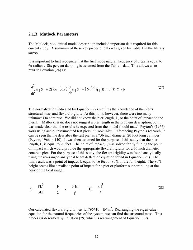
2.1.3 Matlock Parameters The Matlock, et al. initial model description included important data required for this current study. A summary of these key pieces of data was given by Table 1 in the literary survey. It is important to first recognize that the first mode natural frequency of 3 cps is equal to 6π radians. Six percent damping is assumed from the Table 1 data. This allows us to rewrite Equation (24) as:

(27)

The normalization indicated by Equation (22) requires the knowledge of the pier’s structural mass and flexural rigidity. At this point, however, there were too many unknowns to continue. We did not know the pier length, L, or the point of impact on the pier, l. Matlock, et al. does not suggest a pier length in the problem description, but it was made clear that the results he expected from the model should match Peyton’s (1966) work using actual instrumented test piers in Cook Inlet. Referencing Peyton’s research, it can be seen that he describes the test pier as a “36 inch diameter, 20 foot long cylinder” (Peyton, 1966, p.140). It was then assumed for the purpose of this study that the pier length, L, is equal to 20 feet. The point of impact, l, was solved for by finding the point of impact which would provide the appropriate flexural rigidity for a 36 inch diameter concrete pier. For the purpose of this study, the flexural rigidity was found analytically using the rearranged analytical beam deflection equation found in Equation (28). The final result was a point of impact, l, equal to 16 feet or 80% of the full height. The 80% height seems like a realistic point of impact for a pier or platform support piling at the peak of the tidal range.

(28)

Our calculated flexural rigidity was 1.1796*1011 lb*in2. Rearranging the eigenvalue equation for the natural frequencies of the system, we can find the structural mass. This process is described by Equation (29) which is rearrangement of Equation (19).

2tη1 t( )d

d

22 .06( ) 6π( )⋅

tη1 t( )d

d⋅+ 6π( )2

η1 t( )⋅+ F t( ) Y1 l( )⋅

ζFL3

3EI

Fζ

k3 EI⋅

l3 EI

k l3⋅3

18

mβ r L⋅( )4 EI⋅

ωr2 L4⋅

(29) 2.1.4 Solution At this point, having acquired the necessary system parameters, the normalization suggested by Equation (21) can be carried out. This normalization leaves us with a value for the constant A1 of 0.0426. Knowing this constant allows us to develop an equation for the fundamental eigenfunction/mode shape equation based on Equation (16). The next step was to formulate a deformation equation of motion at the point of ice impact to verify that it matched the Matlock, et al. version. Using Equation (27) and the newfound knowledge of the fundamental mode shape at the point of impact, Y1(l), we can develop the modal deflection equation shown by Equations (30 a, b). The second equation is the same as the first except that the entire equation has been multiplied by 50000/36π^2. This step was performed in order to match the individual terms to those provided by Matlock.

(30a)

(30b)

It is important to recognize that Equations (30 a, b) do not calculate the deformation at a specific point on the pier unless multiplied by the normalized mode shape value at the vertical point of interest. This is accomplished through the use of Equation (25). Equation (31) shows an equation which closely matches the Matlock point of impact deformation equation thereby verifying the work done to this point. The only minor difference between Equation (31) and the expected Matlock equation of motion is that the forcing is not multiplied by exactly one. This error is due to the use by this study of the analytical beam equation to save calculation time. The effect of this simplifying assumption is minor enough to accept the stated result.

ωr β r L⋅( )2 EI

m L4⋅⋅

2tη1 t( )d

d

22.26

tη1 t( )d

d⋅+ 36π

2η1 t( )+ F t( ) .0842⋅

1402tη1 t( )d

d

2316.4

tη1 t( )d

d⋅+ 50000η1 t( )+ F t( ) 11.85⋅

19

(31)

It is important to note however that the production of Equation (31) was done merely to validate the work done thus far and will not be used in the ordinary differential equation simulators. A more close representation of the equation used for our one mode solution is displayed by Equation (32). One interesting difference to note between Equations (31) and (32) is that Equation (32) is a more capable forced modal response equation. This is accomplished through the use of the multiplication factor/variable mass normalized mode shape specified in Equation (20). We are no longer focused on the deformation at a single spatial coordinate, but rather have made possible a total structure vibration analysis.

2tq1 t( )d

d

22.26

tq1 t( )d

d⋅+ 355.3q1 t( )+ Y1 l( ) Y1 x( )⋅ F t( )

(32) The selection of the integrator is of great importance when trying to develop a time series for this model. MATLAB generally recommends the use of the ODE45 solver, but the one caveat is that this particular solver does not fare well with stiff problem types. By a stiff ODE we mean an ODE for which numerical errors compound dramatically over time. For example, consider the ODE: y′ = −2000y + 2000t + 1. Since the dependent variable, y, in the equation is multiplied by 2000; small errors in our approximation will tend to become magnified. In general, we must take considerably smaller steps in time to solve stiff ODEs, and this can lengthen the time to solution. Often, solutions can be computed more efficiently using one of the solvers designed for stiff problems. The stiff nature of the equations of motion led to the selection of a MATLAB ode15s solver which is a stiff solver with medium accuracy. A MATLAB script ‘ice’ was developed simulate the ice model. Some interesting analysis tools were programmed into “ice” including: • Array that records time, structural displacement and structural velocity at the point of

any ice tooth fracture • Array that records time and structural displacement at any loss of contact between

moving ice floe and structure. Another program, ‘iceproject’ was developed to: • Allow user input of ice velocity, number of modes to use in the analysis, type of

output requested and time to run the simulation • Plot deformation time series at any point along pier or several at once in subplots • Overlay tooth fracture and loss of contact over any time series • Plot Poincaré Maps using points in phase plane that correspond to tooth breakage

(Karr, et al. 1992) which can help us discover periodic orbits

1402tq1 t( )d

d

2316.4

tq1 t( )d

d⋅+ 50000q1 t( )+ .998F t( )

20

• Plot Local Recurrence Plots based on work of Hegger, Kantz, and Schreiber (1999) and Dr. Charles L. Webber, Jr. (1996)

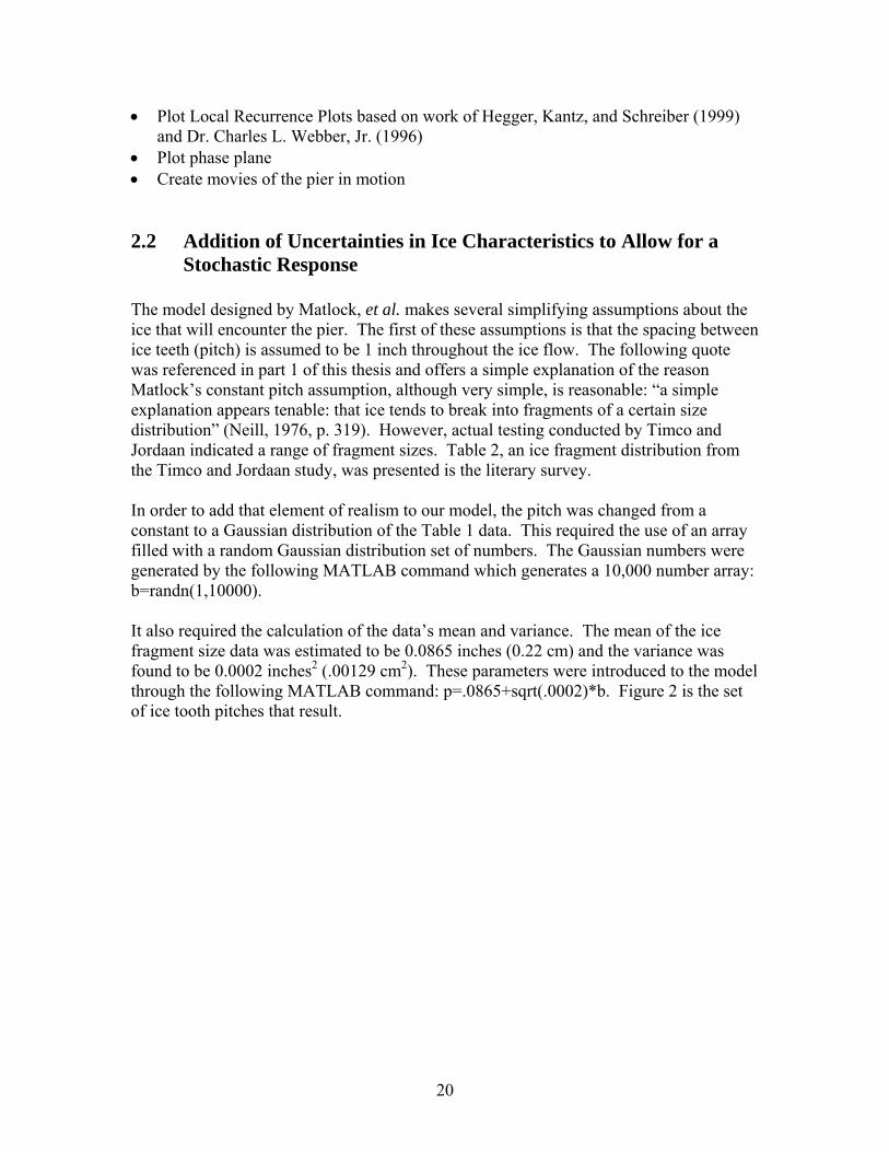
• Plot phase plane • Create movies of the pier in motion 2.2 Addition of Uncertainties in Ice Characteristics to Allow for a Stochastic Response The model designed by Matlock, et al. makes several simplifying assumptions about the ice that will encounter the pier. The first of these assumptions is that the spacing between ice teeth (pitch) is assumed to be 1 inch throughout the ice flow. The following quote was referenced in part 1 of this thesis and offers a simple explanation of the reason Matlock’s constant pitch assumption, although very simple, is reasonable: “a simple explanation appears tenable: that ice tends to break into fragments of a certain size distribution” (Neill, 1976, p. 319). However, actual testing conducted by Timco and Jordaan indicated a range of fragment sizes. Table 2, an ice fragment distribution from the Timco and Jordaan study, was presented is the literary survey. In order to add that element of realism to our model, the pitch was changed from a constant to a Gaussian distribution of the Table 1 data. This required the use of an array filled with a random Gaussian distribution set of numbers. The Gaussian numbers were generated by the following MATLAB command which generates a 10,000 number array: b=randn(1,10000). It also required the calculation of the data’s mean and variance. The mean of the ice fragment size data was estimated to be 0.0865 inches (0.22 cm) and the variance was found to be 0.0002 inches2 (.00129 cm2). These parameters were introduced to the model through the following MATLAB command: p=.0865+sqrt(.0002)*b. Figure 2 is the set of ice tooth pitches that result.

21

0 1000 2000 3000 4000 5000 6000 7000 8000 9000 100000.02

0.04

0.06

0.08

0.1

0.12

0.14P

itch

(inch

es)

Gaussian Pitch-10000 Number Array

Figure 2. Gaussian Distribution of Pitch Matlock, et al. also assumed that the maximum static ice force is 450 kips, which is held constant throughout the analysis. In an effort to achieve greater realism, calculations were performed using the technique described by Eranti and Lee (1986). This technique was explained in the literary survey. The maximum static ice forces were found to result from a ductile failure mode of the ice. Table 4 lists the values that were input into Equation (4).

Table 4. Input for Ductile Failure Equation Variable Value

σc 125 lb/in2 (Neill, 1976) k 0.8 m 0.9 n 1.0 f 2, 3, 4, 5 D 36 in (Peyton, 1966) h 3.5 ft (Peyton, 1966)

The resulting maximum static ice forces for the four different strength factors are given below.

22

It is interesting to note that testing cited by Eranti and Lee (1986) and conducted by Michel and Toussaint (1976) “determined empirically that a value of 2.97 for f gave reasonable agreement between indentation and uniaxial tests for columnar grained S2 ice over the entire strain-rate range at -10°C (14°F)” (Eranti and Lee, 1986, p.113). The maximum static ice force calculated at a strength factor of 3 was 408.2 kips which is remarkably close to the value chosen by the Matlock, et al. study. This lends some credibility to the Matlock, et al. study. However, as cited by Eranti and Lee (1986), Frederking (1977) found that “columnar grained ice samples were two to five times stronger when lateral deformation was prevented than in normal uniaxial tests” (Eranti and Lee, 1986, p.112). This was the reasoning for calculating the maximum static ice forces at the other strength factors. While this range of peak forces exists, it seems more appropriate that they exist as a Gaussian distribution centered at 408.2 kips, the value at the strength factor of three. It was also determined that the force required to cause ductile failure may be related to the ice tooth pitch. The force required was hypothesized to increase based on an increase in the fragment size of ice currently being fractured. The two variables were related by using the same random Gaussian distribution given before as: b=randn(1,10000). The mean was calculated to be 408.2 kips with a variance of 1.3*109 lbs2. These parameters were introduced to the model through the following MATLAB command: force=4.082*105+sqrt(1.3*109)*b. Figure 3 is the set of maximum ice forces that result.

F

2.722 105×

4.082 105×

5.443 105×

6.804 105×

⎛⎜⎜⎜⎜⎜⎜⎝

⎞⎟⎟⎟⎟⎟⎟⎠

lbf=

23

0 1000 2000 3000 4000 5000 6000 7000 8000 9000 100002.5

3

3.5

4

4.5

5

5.5x 10

5

Max

imum

Ice

Forc

e (lb

s)

Gaussian Forces-10000 Number Array

Figure 3. Gaussian Distribution of Maximum Ice Forces 2.3 Addition of Ice Accumulation on the Pier Modeled as a Point Mass Many of the studies referenced by this work indicate the possibility of rubble formation in front of the pier. “When ice begins to fail against a wide structure, it will not generally clear away. Broken ice accumulates and eventually forms a rubble in front of the structure” (Eranti and Lee, 1986, p. 133). These rubble formations have the potential for freezing together and becoming a point mass on the modeled pier. It became a goal of this study to add a point mass at the ice floe height of impact that would change the dynamics of the ice-structure interaction. This is portrayed in Figure 4, a sketch of the pier.

24

Figure 4. Sketch of ice accumulation on pier at impact height adapted from Matlock, et al. (1969, 1971) 2.3.1 Modal Analysis A. Beam Equation

25

This process can be started with the beam equation in Equation (12a). That equation was used for our solution without a point mass on the pier. The objective of the current analysis is to be able to place a point mass of ice at any height on the pier. In this case, the pier has to be divided into two segments-from 0 to height of impact and from height of impact to the top of the pier. The segmentation of the pier is required because of the discontinuity of the point mass at impact height. In order to accomplish that objective, two differential equations must be developed for the two parts of the beam. The solution to the two differential equations is given by:

(33)

This analysis requires 8 boundary conditions to be applied. These boundary conditions are: (a) Y1(0) = 0 deflection at clamped end is zero (b) Y1′(0) = 0 slope of the deflection curve at clamped end is zero (c) Y1(l) = Y2(l) displacement continuity at impact height (d) Y1′(l) = Y2′(l) slope continuity at impact height (e) Y1′′(l) = Y2′′(l) bending moment continuity at impact height (f) Y1′′′(l) + M/m*β4*Y1(l) = Y2′′′(l) shear force discontinuity due to inertial force of the point mass (g) Y2′′(L) = 0 bending moment at free end is zero (h) Y2′′′(L) = 0 shear force at free end is zero It is important to understand that m is the distributed mass of the pier while M is the point mass of ice. B. Normality One major difference in this analysis is the method of mass normalizing the mode shapes. The null vector is the vector of constants A-H that when multiplied by the terms of the 8 boundary conditions returns a 8 by 1 matrix of zeros. This null vector was found for each impact height by substituting the first eigenvalue, Β1L, into the matrix of boundary conditions. The command “condest” in MATLAB, which finds the null vector, was then used on the matrix. The null vector is substituted into Equation (33) for A through H completing the two differential equations with the exception of the constant Cr. After obtaining the null vector it is possible to mass normalize the mode shapes in the following manner and find the value of the constant Cr:

Y2.r x( ) Cr E sin β r x⋅( )⋅ F cos β r x⋅( )⋅+ G sinh β r x⋅( )⋅+ H cosh β r x⋅( )⋅+( )⋅

Y1.r x( ) Cr A sin β r x⋅( )⋅ B cos β r x⋅( )⋅+ C sinh β r x⋅( )⋅+ D cosh β r x⋅( )⋅+( )⋅

26

0

lxm x( ) Y1.r x( )( )2⋅

⌠⎮⌡

dl

Lxm x( ) Y2.r x( )( )2⋅

⌠⎮⌡

d+ M Y1.r l( )( )2⋅+ 1

(34)

2.3.2 Parameters It became necessary to calculate a realistic mass of this frozen rubble formation. Based on an array of photographs and observations from other studies, a set of dimensions of the ice point mass was developed. The shape of the ice point mass was assumed to be a sloped pile that covers the front half perimeter of the pier. The dimensions included a sloped section 48 inches high with a 6 inch base. The pier radius is 18 inches as defined by Peyton (1966). Given the density of sea ice of 0.9 tonne/m3 or 0.033 lb/m3, we are able to calculate the mass based on overall ice volume. The results are shown by Table 5.

Table 5. Volume and mass of ice point mass Variable Result

V=1/2*b*h* π*r 8.143*103 in3 M=V* ρ 264.8 lb

2.3.3 Solution and Validation of Model After applying these new boundary conditions, it is possible to solve for the zeros of the matrix determinant. The eigenvalues for three different impact heights are displayed in Table 6.

27

Table 6. First 10 Eigenvalues at Three Different Point Mass/Impact Locations Eigenvalues Impact 120 inch Impact 160 inch Impact 192 inch

β 1 L⋅

1.7159 1.5616 1.4393

β 2 L⋅ 3.8141 4.3703 4.6867

β 3 L⋅ 7.8538 7.0455 7.4498

β 4 L⋅ 9.7931 10.9213 10.0043

β 5 L⋅ 14.1372 13.3115 13.4309

β 6 L⋅ 15.9531 16.2063 17.0665

β 7 L⋅ 20.4204 20.3261 20.3645

β 8 L⋅ 22.1743 22.6805 22.4315

β 9 L⋅ 26.7035 25.5826 25.3785

β 10 L⋅ 28.4203 29.7467 29.0355

Using these newly found eigenvalues, and the eigenfunctions/modeshapes for each of the two beam segments a modal analysis can be performed with the addition of the point mass. The two-beam model was validated through a two-prong test:

1. Set non-dimensional quantity M/(m*L) to zero by making the point mass, M, equal to zero. Set impact height to 120 inches so that l/L=0.5. Beam eigenvalues should be the same as the one beam model with no point mass.

2. Set non-dimensional quantity M/(m*L) to 1. Set impact height to the top of the pier so that l/L=1. Beam eigenvalues should match textbook values for a one beam model with a tip mass.

The MATLAB two beam analysis was properly validated as a functional design through successful comparison with previously calculated one-beam model eigenvalues.

28

Chapter 3-Application of Modal Analysis to the Model and Typical Results 3.1 Replication of Previous Model Simulations To validate the modal analysis, single mode simulations are compared to the Matlock (1969, 1971) result. Matlock ran simulations of the model for typical high and low ice velocities and compared the results with existing laboratory and field measurements. For comparison purposes, single mode simulations were run with the Matlock, et al. variables for the same time series lengths. The first such simulation for a low ice velocity of 5 inches/second is shown in Figure 4.

0 2 4 6 8 10 12-2

0

2

4

6

8

10

time(sec)

Stru

ctur

e D

ispl

.(in)

Ice Velocity: 5 in/sec. 192 in. from beam btm/ 1 mode solution.

Structural DisplacementBroken TeethLoss of Contact

Figure 5. Single Mode Simulation-Low Velocity Ice Flow The simulation shown by this figure is at the characteristic impact height of 16 feet or 80% of the pier length, a set point calculated in part two of this work. In Figure 4, broken ice teeth are indicated by red asterisks and loss of contact between ice and structure is shown by a blue circle. The one mode, low velocity ice plot is in close agreement with Matlock’s (1969, 1971) results, but there are some noticeable differences. The

29

similarities include the dominance of the expected saw-tooth deflection, a maximum deflection of approximately nine inches and the equal periodicity of motion. The periodic motion is seen to match the expected result by displaying the same number of characteristic saw-tooth excursions in the eleven second simulation. The noticeable differences include a slight difference in the number of teeth broken per excursion and more variance in the peak heights of the saw-tooth excursions. The overall rate of tooth fracture remains as expected at approximately five fractures per second, but does not match the expected behavior of exactly nine tooth fractures per structural return. The variance in peak height and number of tooth fractures appears to be a more realistic approximation and is echoed by the work of Karr, et al. These differences are minute and most likely due to differences in time-steps used by the ordinary differential equation simulator. Smaller time increments are required by the model due to its stiffness and errors can result if the integration tool used does not accommodate this. The loss of contact plot enables us to analyze and understand the regime of structural loading immediately following structural return. The frequency at which the structure vibrates is not the natural frequency and went largely unexplained in previous work. Close examination of Figure 4 indicates that this frequency is a characteristic of contact between ice and structure. During periods of contact loss a periodic motion similar to the structure’s natural frequency of three cycles per second is seen. As contact is regained a much higher frequency of pier motion, approximately equal to ten cycles per second, is seen that is characteristic to the ice-structure interaction. This is an important observation that offers potential for future studies that identify the exact frequency of this characteristic of the contact. A single mode simulation of the pier motion at a high ice velocity of 50 inches/second is shown in Figure 5. There were once again many similarities with the simulation presented by Matlock, et al. Figure 5 displays the existence of sustained “superimposed oscillation at the structure natural frequency” (Matlock, et al., 1969, p.690) with a mean value of 4.5 inches. The oscillation at the structure’s natural frequency can be explained by the loss of contact overlay in which it can be seen that the structure is more frequently out of contact with the ice. This allows for vibration as a characteristic of the structure alone. The tooth fracture rate averages 50 per second as observed by previous studies. The key difference between the one mode approximations is in the amplitude of oscillation. Previous studies of the one mode approximation showed eventual settling into a continuous, small amplitude interaction about the 4.5 inch mark of approximately +/- 0.5 inches. The behavior of the interaction in Figure 5 shows a much larger amplitude of oscillation about the 4.5 inch mean deflection of approximately +/- 4 inches. This large variation was a cause for concern in the accuracy of the simulation and prompted further analysis. Another simulation was run with 100 equal time steps, bypassing the power of the Matlab ode15s simulation to decrease time increments in those areas needed. The result was very close to the Matlock, et al. approximation and did not include the level of detail displayed by Figure 5. The one inch oscillation was seen to exist in this version of the simulation. This lent further credibility to my assertion of potential errors in earlier simulations associated with time-step increments.

30

0 0.5 1 1.5 2 2.5 3-1

0

1

2

3

4

5

6

7

8

9

time(sec)

Stru

ctur

e D

ispl

.(in)



Figure 6. Single Mode Simulation-High Velocity Ice Flow 3.2 Extension of Model to Show Single Mode Displacements at Multiple Vertical Pier Locations Having successfully verified the model via comparison with Matlock’s result, it will be used for a total structure vibration analysis. It was decided to start with a multi-location single mode approximation in order to display the value of a total pier approach. Figure 7 shows a low ice velocity, 5 inches/second, simulation with all of the same parameters used for previous single location runs. The interest in pursuing this type of plot is in showing that the previous one location plot can be seen as the 192 inch from beam bottom plot in a multi-location plot. We have lost none of the realism of previous renditions and increased the user’s ability to see the plots as an actual structure.

31

0 1 2 3 4 5 6 7 8 9 10 110

5

10

time(sec)

Stru

ctur

e D

ispl

.(in)


Structural Displacement

0 1 2 3 4 5 6 7 8 9 10 110

5

10

time(sec)

Stru

ctur

e D

ispl

.(in)



0 1 2 3 4 5 6 7 8 9 10 110

5

10

time(sec)

Stru

ctur

e D

ispl

.(in)



0 1 2 3 4 5 6 7 8 9 10 110

5

10

time(sec)

Stru

ctur

e D

ispl

.(in)



Figure 7. Single Mode Multi-Location Simulation-Low Velocity Ice @ 192 in. Some interesting observations can be made from the multi-location plots. While it may seem obvious and trivial, the location on the pier greatly affects the level of displacement/forcing felt. While a 9 inch peak is characteristic at the set impact height of 192 inches, peak values are shown to vary between 1.2 inches and 12.4 inches elsewhere on the pier vertically. The periodic motion as expected is the same throughout the pier. Figure 8 shows a high ice velocity, 50 inches/second, simulation with all of the same parameters used for previous single location runs.

32

0 0.5 1 1.5 2 2.5 30

5

10

time(sec)

Stru

ctur

e D

ispl

.(in)



0 0.5 1 1.5 2 2.5 30

5

10

time(sec)

Stru

ctur

e D

ispl

.(in)



0 0.5 1 1.5 2 2.5 30

5

10

time(sec)

Stru

ctur

e D

ispl

.(in)



0 0.5 1 1.5 2 2.5 30

5

10

time(sec)

Stru

ctur

e D

ispl

.(in)



Figure 8. Single Mode Multi-Location Simulation-High Vel. Ice @ 192 in. The mean value about which the structure oscillates remains at 4.5 inches at the impact site, but varies between 0.5 inches and 6 inches as you move up the pier vertically. The periodic motion at the structure’s natural frequency remains characteristic of the total pier vibration. The total pier picture offered by this multi-location plot allows for a much more detailed vibration analysis that includes multiple mode shapes interacting to increase and decrease the displacement/forcing along the pier length. If the entire pier is not considered, the whole picture cannot be seen. While it may be obvious for the single mode approach that the displacements will vary in a simple one mode shape, this is not the case for a more realistic multi-mode approach. 3.3 Multi-Mode Approximations at Multiple Pier Locations Having decided that it would be of great value to pursue a multi-location, multi-mode response the Matlab program was modified to apply up to 20 modes to the system response. The number of modes to be used was designed as a user input along with the ice velocity. As stated in Chapter 2, the use of modal analysis allows us to: 1. Find the structure’s natural modes and natural frequencies. 2. Calculate each individual mode’s response.

33

3. Find the full modal response to a given loading. One of the program’s primary functions is to calculate the natural frequencies of the pier at different modes. The natural frequencies are vital in that they become part of each modal response equation of motion. The modal frequencies calculated by the program are shown in Table 7.

Table 7. Modal Frequencies Mode # Wn (rad/s) Mode # Wn (rad/s)

1 18.8496 11 5831.1412 2 118.1291 12 7019.5522 3 330.7673 13 8267.4972 4 648.16 14 9635.6615 5 1071.4676 15 11118.2979 6 1600.5875 16 12706.9875 7 2242.0169 17 14404.5091 8 2973.2681 18 16204.2946 9 3817.567 19 18099.4058 10 4770.4436 20 20115.709

The calculation of the above frequencies and simulation of the individual mode responses completes the first two elements of modal analysis. In order to acquire the total picture, the time function result must be multiplied by the mass normalized mode shape at each point of interest. The summation of these products provides the full modal response. A simulation was run using all twenty available modes and a low velocity ice flow in order to see the result of this detailed analysis. This simulation can be seen in Figure 9. Figure 10 is a close-in view of the behavior at impact level for comparison with the one mode approximation.

34

0 1 2 3 4 5 6 7 8 9 10 110

5

10

time(sec)

Stru

ctur

e D

ispl

.(in)



0 1 2 3 4 5 6 7 8 9 10 110

5

10

time(sec)

Stru

ctur

e D

ispl

.(in)



0 1 2 3 4 5 6 7 8 9 10 110

5

10

time(sec)

Stru

ctur

e D

ispl

.(in)



0 1 2 3 4 5 6 7 8 9 10 110

5

10

time(sec)

Stru

ctur

e D

ispl

.(in)



Figure 9. Twenty Mode Multi-Location Simulation-Low Vel. Ice @ 192 in. Some interesting observations from Figure 9:

• Peak height variance between 1.21 inches and 12.45 inches (1 mode was 1.2 inches-12.4 inches)

• Higher frequency of saw-tooth behavior (extra peak within 11 second simulation) • Averages same 5 tooth fracture/sec rate even though there are more saw-tooth

cycles (more evolutions that do not reach 9 inch characteristic deflection-less stored energy for return)

• The periodic repeating of the saw-tooth behavior is seen at each height of the pier/pile. As expected, the simulated structure acts as one pier.

35

0 2 4 6 8 10 120

1

2

3

4

5

6

7

8

9

10

time(sec)

Stru

ctur

e D

ispl

.(in)



Figure 10. Twenty Mode Impact Location Simulation-Low Vel. Ice @ 192 in. Observations from impact location plot in Figure 10:

• During periods of contact loss a periodic motion similar to the structure’s natural frequency of three cycles per second is still seen. As contact is regained a much higher frequency of pier motion, approximately equal to ten cycles per second, is also still seen that is characteristic to the ice-structure interaction.

• Clarity is added to the plot. The use of multiple modes, decreases the time step size required by the MATLAB program. This enables us to see that loss of contact is near constant in some areas of the plot and imminently closer to fracture points. Note: Fracture points and loss of contact never occur simultaneously although it appears that way in this plot.

A simulation was run using twenty modes and a high velocity ice flow in order to see the result of this detailed analysis. This simulation can be seen in Figure 11. Figure 11 is a close-in view of the behavior at impact level for comparison purposes.

36

0 0.5 1 1.5 2 2.5 30

2

4

6

time(sec)

Stru

ctur

e D

ispl

.(in)



0 0.5 1 1.5 2 2.5 30

2

4

6

time(sec)

Stru

ctur

e D

ispl

.(in)



0 0.5 1 1.5 2 2.5 30

2

4

6

time(sec)

Stru

ctur

e D

ispl

.(in)



0 0.5 1 1.5 2 2.5 30

2

4

6

time(sec)

Stru

ctur

e D

ispl

.(in)



Figure 11. Twenty Mode Multi-Location Simulation-High Vel. Ice @ 192 in. Some interesting observations from Figure 11:

• The mean value about which the structure oscillates is 4.691 inches at the impact site, but varies between 0.62 inches and 6.5 inches (one mode was 0.5 inches and 6 inches) as you move up the pier vertically.

• The periodic motion at the structure’s natural frequency remains characteristic of the total pier vibration, but ends at about 1 second. After the first second, a small amplitude vibration about the mean displacement of +/-.01 to +/-.05 inches dominates. This small amplitude vibration oscillates at a rate of approximately 50 cycles per second. Based on the results of multiple simulations, this appears to be the high velocity ice system characteristic vibration at the pier’s 80% impact height. The previous line of thinking was that repeated loss of contact would cause the structure to vibrate at its natural frequency. While this did appear to happen at first, the faster ice velocity does not allow sufficient contact loss time to maintain this behavior. The initial behavior was due to an initial impact extended loss of contact which triggered the natural frequency of the structure. The displacement/forcing became steady at the characteristic deflection of 4.68 inches with very little oscillation. This can be seen up close in Figure 12.

37

0 0.5 1 1.5 2 2.5 30

1

2

3

4

5

6

time(sec)

Stru

ctur

e D

ispl

.(in)



Figure 12. Twenty Mode Impact Location Simulation-High Vel. Ice @ 192 in. The plots provided by the full modal response provide a great deal more insight and detail into the response. The differences from the fundamental mode solution justify the use of the multi-mode approach and provide impetus for further improvements in realism. 3.4 Variance of Ice Impact Height Due to Tidal Variances The waterway upon which the model is based is Cook Inlet, Alaska. The region is known to have “35 foot tides” (Peyton 1966, p.136). This incredible tidal range brought on the question of the impact of tide changes on the model. Up to this point, the surface ice was assumed to collide with the pier at the 80% height or 16 feet from the seafloor. It was decided that the analysis of this work would make an attempt at understanding the impact of the tidal differences by simulating different ice impact heights ranging from the 10 foot mark (50%) up to the design height of 80%. Specifically, with the 80% design height already fully evaluated, the two impact heights to be examined are 120 inches and 160 inches from the seafloor. Figure 13 shows a simulation of the low ice velocity impacting at 120 inches from the seafloor. Figure 14 shows the modal response at the 120 inch impact height up close. Ten modes were used for each simulation. It was discovered during the course of the analysis that the latter modes have very little effect and that a 10 mode simulation is sufficient as a time saving measure.

38

0 1 2 3 4 5 6 7 8 9 10 110

2

4

time(sec)

Stru

ctur

e D

ispl

.(in)



0 1 2 3 4 5 6 7 8 9 10 110

2

4

time(sec)

Stru

ctur

e D

ispl

.(in)



0 1 2 3 4 5 6 7 8 9 10 110

2

4

time(sec)

Stru

ctur

e D

ispl

.(in)



0 1 2 3 4 5 6 7 8 9 10 110

2

4

time(sec)

Stru

ctur

e D

ispl

.(in)



Figure 13. Ten Mode Multiple Location-Low Vel. Ice @ 120 in. Height

39

0 2 4 6 8 10 120

0.5

1

1.5

2

2.5

time(sec)

Stru

ctur

e D

ispl

.(in)



Figure 14. Ten Mode Impact Location-Low Vel. Ice @ 120 in. Height Observations from Figure 13 and Figure 14:

• Peak height variance between 0.67 inches and 5.52 inches including only 2.15 inches at the impact height (large difference from impact at 192)

• Much greater frequency of saw-tooth behavior (14 extra peaks within 11 second simulation) although the behavior is not the typical saw-tooth behavior.

• Averages same 5 tooth fracture rate/sec even though there are more saw-tooth cycles (none of the evolutions reach 9 inch characteristic deflection-less stored energy for return)

• Periodic motion is the same throughout the pier although not as easily definable as the impact at 192 inches. This impact height will be interesting for further analysis into its periodic motion.

The impact height of 120 inches was then tested with a simulated collision with a high velocity ice flow. Figure 15 is the multiple location plot for the impact at 120 inches and Figure 16 shows the modal response at the 120 inch impact height up close.

40

0 0.5 1 1.5 2 2.5 30

2

4

time(sec)

Stru

ctur

e D

ispl

.(in)



0 0.5 1 1.5 2 2.5 30

2

4

time(sec)

Stru

ctur

e D

ispl

.(in)



0 0.5 1 1.5 2 2.5 30

2

4

time(sec)

Stru

ctur

e D

ispl

.(in)



0 0.5 1 1.5 2 2.5 30

2

4

time(sec)

Stru

ctur

e D

ispl

.(in)



Figure 15. Ten Mode Multiple Location-High Vel. Ice @ 120 in. Height

41

0 0.5 1 1.5 2 2.5 30

0.5

1

1.5

2

2.5

time(sec)

Stru

ctur

e D

ispl

.(in)



Figure 16. Ten Mode Impact Location-High Vel. Ice @ 120 in. Height Observations from Figure 15 and Figure 16:

• The mean value about which the structure oscillates is 1.1 inches at the impact site, but varies between 0.34 inches and 2.841 inches as you move up the pier vertically.

• The periodic motion at the structure’s natural frequency remains characteristic of the total pier vibration, but ends at about 3 seconds as the ice starts overcoming the pier’s natural frequency and the fracture rate picks up. After the first three seconds, a small amplitude vibration about the mean displacement of +/-.01 to +/-.05 inches dominates. This small amplitude vibration seems to oscillate much more frequently at a rate of 45 cycles per second. The displacement/forcing became steady at the characteristic deflection of 1.1 inches with very little oscillation. This can be seen up close in Figure 16.

Figure 17 shows a simulation of the low ice velocity impacting at 160 inches from the seafloor. Figure 18 shows the modal response at the 160 inch impact height up close. Ten modes were used for each simulation.

42

0 1 2 3 4 5 6 7 8 9 10 1102468

time(sec)

Stru

ctur

e D

ispl

.(in)



0 1 2 3 4 5 6 7 8 9 10 1102468

time(sec)

Stru

ctur

e D

ispl

.(in)



0 1 2 3 4 5 6 7 8 9 10 1102468

time(sec)

Stru

ctur

e D

ispl

.(in)



0 1 2 3 4 5 6 7 8 9 10 1102468

time(sec)

Stru

ctur

e D

ispl

.(in)



Figure 17. Ten Mode Multiple Location-Low Vel. Ice @ 160 in. Height

43

0 2 4 6 8 10 120

1

2

3

4

5

6

time(sec)

Stru

ctur

e D

ispl

.(in)



Figure 18. Ten Mode Impact Location-Low Vel. Ice @ 160 in. Height

Observations from Figure 17 and Figure 18:

• Peak height variance between 0.96 inches and 9.1 inches including only 5.25 inches at the impact height (large difference from impact at 192)

• Much greater frequency of saw-tooth behavior (8 extra peaks within 11 second simulation). Behavior more closely resembles saw-tooth form than at 120 inch impact site.

• Averages same 5 tooth fracture rate/sec even though there are more saw-tooth cycles (none of the evolutions reach 9 inch characteristic deflection-less stored energy for return)

• Periodic motion is the same throughout the pier. Contact loss is not as much of a factor in this simulation as in the impact at 192 inches. As contact is almost constant a much higher frequency of pier motion, approximately equal to 7 cycles per second, is seen that is characteristic to the ice-structure interaction.

The impact height of 160 inches was then tested by a simulated collision with a high velocity ice flow. Figure 19 is the multiple location plot for the impact at 160 inches and Figure 20 shows the modal response at the 160 inch impact height up close. The broken teeth are not shown on this plot in an effort to remain consistent with regard to the heights plotted. The impact height is not plotted.

44

0 0.5 1 1.5 2 2.5 30

5

10

time(sec)

Stru

ctur

e D

ispl

.(in)



0 0.5 1 1.5 2 2.5 30

5

10

time(sec)

Stru

ctur

e D

ispl

.(in)



0 0.5 1 1.5 2 2.5 30

5

10

time(sec)

Stru

ctur

e D

ispl

.(in)



0 0.5 1 1.5 2 2.5 30

5

10

time(sec)

Stru

ctur

e D

ispl

.(in)



Figure 19. Ten Mode Multiple Location-High Vel. Ice @ 160 in. Height

0 0.5 1 1.5 2 2.5 3-1

0

1

2

3

4

5

6

7

time(sec)

Stru

ctur

e D

ispl

.(in)



Figure 20. Ten Mode Impact Location-High Vel. Ice @ 160 in. Height

45

Observations from Figure 19 and Figure 20:

• The mean value about which the structure oscillates is 3 inches at the impact site, but varies between 0.46 inches and 4.88 inches as you move up the pier vertically.

• The periodic motion at the structure’s natural frequency remains characteristic of the total pier vibration throughout the time series. This phenomenon will be interesting to examine in greater detail as the structure does not succumb to the faster ice velocity. The cyclic vibration has a larger amplitude about the mean displacement of +/-.561 to +/-5.44 inches dominates. This can be seen up close in Figure 20.

3.5 Periodic Solutions and the Use of Poincaré Maps During much of the previous work, it became obvious that there may be periodic solutions that describe the behavior of the model. Finding and understanding when to expect periodic orbits based on initial system parameters can be very important. When estimating the fatigue life of a bridge/fixed platform pier, the following three pieces of information are key factors:

• “Number of cycles estimated for a given time span • Average contact forces • Magnitudes of the oscillating contact forces” (Karr, et al. 1992, p.231).

All three of these key design components can be better understood by examination of the periodic steady state motion. The discovery of periodic solutions can also contribute to a better understanding of the effects of the single pier/pile on a connected pier/pile structure (fixed platform, bridge). 3.5.1 Low Velocity Ice Floe Poincaré Mapping In order to properly analyze the system for periodic solutions, extended timelines are needed in which hundreds of cycles are run. One such extended timeline is shown by Figure 21. Figure 21 is a 200 second time series run at a 192 inch height of impact with a low velocity ice flow. The behavior appears to be following a pattern or periodic solution, but it is difficult to discover the steady state periodicity of the system with any certainty without a useful mapping of the system response. The Poincaré map is a very effective means of mapping the system response. In this case, as defined by Karr, et al., the Poincaré map is a phase plane plot of the structural displacements and velocities that correspond to ice tooth breakage. This mapping is more effective than a mapping at the structure’s natural frequency because of the system’s lack of reliance on the structure’s dynamic properties. The system is primarily reliant on the ice velocity and structural

46

stiffness. These system parameters define the regimes of contact and loss of contact which ultimately produce different characteristic frequencies.

0 20 40 60 80 100 120 140 160 180 2000

1

2

3

4

5

6

7

8

9

10

time(sec)

Stru

ctur

e D

ispl

.(in)



Figure 21. Extended Time History-Low Ice Vel. w/ Impact @ 192 in. Figure 22 is a Poincaré map sampled at tooth breakage for 300 seconds. Interestingly enough, the system has a clearly indicated periodic behavior. There are nine teeth broken before the periodic behavior begins. The elimination of this transient behavior results in 40 fixed points in the phase plane. This enables the defining of the system at an impact height of 192 inches as a P-40 closed orbit. There is some data slightly off of the fixed points. These points converge to the fixed points and are purely transient data that can be eliminated. The largest range around one fixed point is given by the following: +/- .01 in. structural displacement, +/- 1.75 in/sec structural velocity. This seems reasonable when compared to the full range of data. The largest range is in the structural velocity which has a +/- 1.9% variation.

47

1 2 3 4 5 6 7 8 9 10-80

-70

-60

-50

-40

-30

-20

-10

0

10

Structure Displacement(in)

Stru

ctur

e V

eloc

ity(in

/sec

)Poincare Map: 5 in/sec 192 in. from beam bottom/10mode solution.

Broken Teeth

Figure 22. Poincaré Map, Low Ice Velocity @ 192 inch Impact Height The next step was to look for periodic behavior when a low velocity ice flow impacts the structure at the 160 inch level. An extended 100 second time series was plotted for this set of parameters and is shown by Figure 23. Figure 24 is the associated Poincaré map sampled at tooth breakage for 250 seconds. When examining the plot visually, it appears that two different periodic solutions exist. There seems to be a repeating P-5 behavior between 8.5 seconds and 25 seconds and a P-24 behavior immediately following. The use of the Poincaré map however makes it less obvious. The 29 expected points are not shown clearly as there seems to be too much error involved in identifying these points. Although no periodic behavior has been proven to exist, we can still claim success in that we better understand the system’s cyclic behavior including oscillating forces/displacements involved.

48

0 10 20 30 40 50 60 70 80 90 100-1

0

1

2

3

4

5

6

7

time(sec)

Stru

ctur

e D

ispl

.(in)



Figure 23. Extended Time History-Low Ice Vel. w/ Impact @ 160 in.

49

0.5 1 1.5 2 2.5 3 3.5 4 4.5 5 5.5-60

-50

-40

-30

-20

-10

0

10


Stru

ctur

e V

eloc

ity(in

/sec

)

Poincare Map: 5 in/sec 160 in. from beam bottom/10mode solution.

Broken Teeth

Figure 24. Poincaré Map, Low Ice Velocity @ 160 inch Impact Height Another extended simulation was run for a low velocity ice impact at a 120 inch impact height. This 250 second simulation is displayed by Figure 25. A Poincaré map for this 250 second simulation is shown by Figure 26. The extended time series was studied visually and appeared to have a P-13 periodic solution. This was confirmed by the Poincaré map in Figure 25 which shows 13 distinct fixed points in the phase plane. There is a limited amount of transient data before complete convergence to the 13 fixed points is reached. The largest range about a fixed point is a point in which the group of fractures ranges over the following: +/- .01 in. structural displacement, +/- 2.5 in/sec structural velocity. This seems reasonable when compared to the full range of data. The largest range is in the structural velocity which has a +/- 8.3% variation.

50

0 50 100 150 200 250-0.5

0

0.5

1

1.5

2

2.5

3

3.5

4

4.5

time(sec)

Stru

ctur

e D

ispl

.(in)



Figure 25. Extended Time History-Low Ice Vel. w/ Impact @ 120 in.

51

0.8 1 1.2 1.4 1.6 1.8 2 2.2-25

-20

-15

-10

-5

0

5


Stru

ctur

e V

eloc

ity(in

/sec

)


Broken Teeth

Figure 26. Poincaré Map, Low Ice Velocity @ 120 inch Impact Height 3.5.2 High Velocity Ice Floe Poincaré Mapping The Karr, et al. (1992) study did not pursue Poincaré mapping of the high velocity (50 in/sec) ice floes. This was probably due to the overwhelming interest in understanding the destructive low velocity saw-tooth ratcheting behavior. At first glance, the pile’s dynamics at high velocity appear to prescribe to a very simple pattern of sustained deflection at half of the maximum low velocity ice floe caused deflection. However, the previous studies had not been able to examine the dynamics of the pile impacted by the tidal range so prevalent in places such as Cook Inlet, Alaska. The present study of the model showed that the impact location vertically on the pile can and will change the dynamics. The present study elected to pursue Poincaré mapping of the high velocity response time series in an effort to learn more about the anticipated behavior. Figure 27 is the Poincaré map of the response to the 50 in/sec ice floe impact at 192 inches from the pile bottom which takes place over 45 seconds. Perhaps not surprisingly, after some minimal transient behavior, the map converges to a single point. The point of system convergence is centered at 4.691 inches of horizontal deflection at impact height and 0.4199 in/sec of pile velocity indicating some slight movement. This particular example demonstrates the mapping of the high velocity system response of the original model which did not allow for tidal variation. As expected from earlier studies of the

52

Matlock model, the sustained deflection is approximately half of the 9 inch maximum deflection caused by the low velocity ice floe.

4 4.5 5 5.5-2

0

2

4

6

8

10

12

14

16

18


Stru

ctur

e V

eloc

ity(in

/sec

)

p

Broken Teeth

Figure 27. Poincaré Map, High Ice Velocity @ 192 inch Impact Height Figure 28 is the Poincaré mapping and phase plane of the response of the pile impacted at a height of 160 inches from the seafloor which takes place over 55 seconds. The mapping at this impact height justifies the study of the high velocity dynamics and periodicity. The map shows a horseshoe shape and does not converge to a single point. This behavior is interesting because it nearly rivals the violence of the low velocity ratcheting behavior. The motion includes displacements ranging from -0.1888 inches to 6.018 inches, a range of 6.2068 inches. This is not much off the 9 inch maximum at impact height for the low velocity floe. The periodic motion of the pile includes velocities ranging from 46.26 in/sec to -59.78 in/sec. The phase plane on which the Poincaré map is overlaid demonstrates the effect of sampling at ice tooth fracture. Sampling at a different frequency could lead to different results.

53

Figure 28. Poincaré Map Overlaid on Phase Plane, High Ice Velocity @ 160 inch Impact Height Figure 29 is a 45 second Poincaré mapping of the high velocity response at an impact height of 120 inches from the bottom of the pile. The map provides a little more transient behavior than seen at the 192 inch impact location, but it does share one similarity. The mapping of the response at the 120 inch height does converge to a single point. The point of convergence is centered at a horizontal pile deflection of 1.126 inches and a structural velocity of 5.004 in/sec. The velocity of the pile is much higher than the convergence point of the 192 inch impact height. The deflection is about half of the 2.15 inch peak experienced when the pile was struck by a low velocity ice floe at the 120 inch impact height.

54

0.2 0.4 0.6 0.8 1 1.2 1.4 1.6 1.8 2 2.2-30

-20

-10

0

10

20

30

40


Stru

ctur

e V

eloc

ity(in

/sec

)


Broken Teeth

Figure 29. Poincaré Map, High Ice Velocity @ 120 inch Impact Height 3.6 Recurrence Plots The discovery of the interesting periodic nature of the pile’s behavior when impacted by low and high velocity ice floes spurred interest in other methods of identifying structure in the displacement time series. This led the present study to look into the recurrence plot as an option. A recurrence plot is a plot showing, for a given moment in time, the times at which a phase space trajectory visits roughly the same area in the phase space. “Recurrence plots are a useful tool to identify structure in a data set in a time resolved way quantitatively” (Hegger, Kantz and Schreiber 1998, p. 7). The Hegger, et al. work developed a routine recurr as part of their TISEAN software package which was defined as follows: “Our routine recurr simply scans the time series and marks each pair of time indices (i,j) with a black dot, whose corresponding pair of delay vectors has distance ≤ ε. Thus in the (i,j)-plane, black dots indicate closeness” (Hegger, et al. 1998, p.7). The Hegger work also mentioned the color rendering and quantification of recurrence plots offered in software developed by Dr. Charles Webber, Jr. Dr. Webber’s Loyola University Chicago homepage explains that a “local recurrence plot is generated by keeping the radius low (15% of maxdist), allowing recurrences to occur only in near neighborhoods” (Webber 1996). The present study developed an addition to the MATLAB program which generated the time series which follows a scheme similar to that of the Hegger, et al. recurr routine.

55

As a starting point, the pier’s displacement and velocity time series must be in evenly spaced time increments. The time increments normally output from an ordinary differential equation simulation are not evenly spaced and would hinder proper analysis by way of recurrence plot. Two forms of the routine were created; dimensional and non-dimensional. Both dimensional and non-dimensional routines used by the present study start out by finding two maximum differences; between the maximum and minimum point of the displacement data and similarly the maximum difference in the recorded velocity data. The dimensional routine finds the normal vector for the maximum displacement and velocity differences and multiplies it by the neighborhood size desired expressed as a percentage. The result is a percentage/neighborhood size of the normal vector which can be compared to normal vectors of the displacement/velocity vector difference throughout the time series. The routine places the displacement and velocity at each point in time into a displacement/velocity vector. Through the use of for loops, the difference is found between each vector and the vectors associated with the other points in the time series. The normal vector is found for each of these differences and compared to the previously calculated neighborhood sized normal vector. If the normal vector, calculated in the for loop, is less than the neighborhood sized normal vector than the two times are plotted as one point. This gives the study a measure of closeness in the time series. There are some negatives to a dimensional approach to recurrence plotting which will be discussed later. A non-dimensionalized routine was developed to negate the potential errors involved in a purely dimensional analysis. The displacement/velocity vectors in the routine are non-dimensionalized by the max differences calculated previously. Non-dimensionalization makes it possible to compare the normal vectors of the non-dimensional displacement/velocity vector differences directly to a percentage /desired neighborhood size instead of to a normal vector sized prior to the routine. Our recurrence routine utilized the Webber recommended 15% of the maximum distance above the line of identity (LOI) and a smaller 7.5% below the LOI. This set of percentages was used as a starting point. The neighborhood size can be reduced to further filter illegible recurrence plots, much like a reduction filter for marine radar. Plus signs were used instead of black dots and the two sides were colored red and blue to make clear that they are different plots. The end result is a set of local recurrence plots that show the difference in choice of neighborhood size. 3.6.1 Low Velocity Ice Floes As with the Poincaré mapping, we first looked at the recurrence plots of the low (5 in/sec) velocity dynamics. The dimensional data at the 192 inch impact height was determined to be skewed by the large negative velocities in the time series. The large velocities drive the dimensional behavior and yield results dominated by velocity. The dominance by the large velocities was consistent for all impact heights of the low velocity behavior.

56

A non-dimensional approach proved to be more effective. Figure 30 is a non-dimensionalized local recurrence plot of the impact at the 192 inch height. The resulting plot displays several interesting elements which can be interpreted. The first thing that you see when looking at this plot is the obvious diagonal lines parallel to the line of identity (LOI). This is an indication of a similarity between the progressions of states at different times and may indicate a deterministic process. This is not surprising since the Poincaré mapping of the time series data resulted in a clearly defined P-40 orbit. It is also obvious that these lines parallel to the LOI include clustered sections which indicate a slower change of state in the vicinity of the clusters. These are most likely the regimes of the plot in which the pile displacement ramps up slowly before crushing through several ice teeth more rapidly on the return. The spacing between the parallel lines is about equal indicating a set period or time distance between similar evolutions of states. The difference between the 15% plot and the 7.5% plot is seen in between the clusters. The 7.5% plot does not record the faster moving parts of the times series.

Figure 30. Local Recurrence Plot (Non-dimensionalized), Low Ice Velocity @ 192 inch Impact Height Figure 31 is a non-dimensional local recurrence plot of the low velocity impact at the 160 inch height over an 11 second timespan. The Poincaré mapping, Figure 24, of the behavior did not contain a clearly identifiable structure. The plot at the 160 inch height has a similar structure to that seen in Figure 30. The spacing between parallel lines is

57

narrower indicating a smaller period. The clusters exist again showing the slowing of the structure. One difference is that there appears to be more than one period in the resulting behavior. Some of the clusters are located off of the lines. This may help explain the difficulty in ascertaining the periodic behavior via a Poincaré map. The 7.5% plot provides a more clear display of these features by removing some of the clutter from the 15% plot. Reducing the neighborhood size has a filtering effect on the plot.

Figure 31. Local Recurrence Plot (Non-dimensionalized), Low Ice Velocity @ 160 inch Impact Height While Figure 31 does allow for some valuable analysis, the spacing of the periodic structure makes the analysis more difficult than need be. When trying to improve upon an already established recurrence plot, the thought process developed by the present study is as follows:

58

Figure 32. Recurrence Plot Decision Flow Chart Following the decision flow chart, the decision was made to keep the neighborhood size intact and zoom into a section of the plot to improve structure visibility by way of spacing. Figure 33 is non-dimensional local recurrence plot of the 160 inch impact point during the final 4 seconds of the time span in Figure 31. While most of the observations that can be made mirror that of the Figure 31 analysis, it becomes even clearer that there may be more than one frequency involved in the time series.

Structure of previous recurrence plot

visible? (No excessive clutter)

Reduce neighborhood size until structure of

plot is visible. (No excessive clutter)

Is the spacing of the structure acceptable

to provide for meaningful analysis?

Previous Recurrence Plot Acceptable

Repeat Previous StepIs the spacing of the structure acceptable

to provide for meaningful analysis?

New Recurrence Plot Acceptable

Repeat Previous Step

No Yes

NoYes

Yes

No

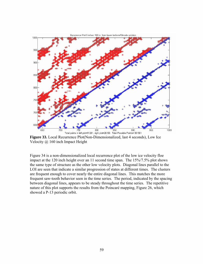
59

Figure 33. Local Recurrence Plot(Non-Dimensionalized, last 4 seconds), Low Ice Velocity @ 160 inch Impact Height Figure 34 is a non-dimensionalized local recurrence plot of the low ice velocity floe impact at the 120 inch height over an 11 second time span. The 15%/7.5% plot shows the same type of structure as the other low velocity plots. Diagonal lines parallel to the LOI are seen that indicate a similar progression of states at different times. The clusters are frequent enough to cover nearly the entire diagonal lines. This matches the more frequent saw-tooth behavior seen in the time series. The period, indicated by the spacing between diagonal lines, appears to be steady throughout the time series. The repetitive nature of this plot supports the results from the Poincaré mapping, Figure 26, which showed a P-13 periodic orbit.

60

Figure 34. Local Recurrence Plot (Non-dimensionalized), Low Ice Velocity @ 120 inch Impact Height Using the Recurrence Plot Decision Flow Chart, the decision was made to zoom in on the last 3 seconds in an effort to increase the spacing of the plot structure. The more focused plot in Figure 35 was the result. Figure 35 shows the existence of at least two frequencies indicated by the different spacing between periodic diagonal lines. There also seems to be some interesting features to the clusters. The clusters are bordered by 2 horizontal and 2 vertical lines each time which can be seen best on the 15% left plot. This is an interesting addition to the periodic behavior discovered through the focused analysis of the flow chart developed by this study.

61

Figure 35. Local Recurrence Plot (Non-dimensionalized, last 3 seconds), Low Ice Velocity @ 120 inch Impact Height 3.6.2 High Velocity Ice Floes The high velocity (50 in/sec) ice floes were also analyzed using the local recurrence plot. There are some challenges associated with recurrence plots of the high ice velocity impact. The displacement and velocity differences can be quite large compared to the rest of the times series. The typical behavior of the pier in high ice velocity floes is a sharp peak of pier displacement at impact followed by a settling to a near constant displacement of about ½ of the peak for the remainder of the time series. The velocity is also known to peak very high at the moment of impact and then oscillate near zero for the reminder of the data set. Another challenge is the more frequent oscillation of the structure under the higher velocity loading. This can make the spacing small enough between periodic lines that a recurrence plot becomes difficult to analyze. The high velocity ice floes, much like the low velocity floes, also provided a challenge for the use of the dimensional analysis. The results were once again dominated by the large velocities in the time series. The largest recorded velocities in the high speed floes are positive and occur at initial impact. The non-dimensional approach was preferred. Figure 36 is the non-dimensionalized local recurrence plot of the high velocity ice floe impact with the pile at the height of 192

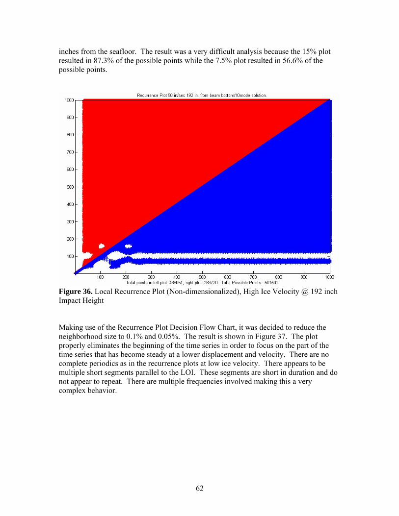
62

inches from the seafloor. The result was a very difficult analysis because the 15% plot resulted in 87.3% of the possible points while the 7.5% plot resulted in 56.6% of the possible points.

Figure 36. Local Recurrence Plot (Non-dimensionalized), High Ice Velocity @ 192 inch Impact Height Making use of the Recurrence Plot Decision Flow Chart, it was decided to reduce the neighborhood size to 0.1% and 0.05%. The result is shown in Figure 37. The plot properly eliminates the beginning of the time series in order to focus on the part of the time series that has become steady at a lower displacement and velocity. There are no complete periodics as in the recurrence plots at low ice velocity. There appears to be multiple short segments parallel to the LOI. These segments are short in duration and do not appear to repeat. There are multiple frequencies involved making this a very complex behavior.

63

Figure 37. Local Recurrence Plot (Non-dimensionalized, reduced neighborhood size), High Ice Velocity @ 192 inch Impact Height Figure 38 is a non-dimensional local recurrence plot of the impact of a high velocity ice floe at the height of 160 inches. This plot is of particular interest because Poincaré mapping, Figure 28, of the fracture behavior at this impact height and ice velocity indicated a horseshoe shaped periodic. The resulting recurrence plot is seemingly the most periodic display of all of the recurrence plots including those at lower ice velocities. The lines are evenly spaced and diagonal to the LOI. There are few noticeable clusters. The display indicates a repeating evolution of states at a periodic pace. There do not appear to be any obvious signs of speeding up or slowing down the rate of change of states. The steady, periodic nature of the behavior is quite different from the expected behavior at high ice velocities.

64

Figure 38. Local Recurrence Plot (Non-dimensionalized), High Ice Velocity @ 160 inch Impact Height Figure 39 is the non-dimensionalized local recurrence plot of the high velocity ice floe impact at the 120 inch height. The plot uses neighborhood sizes of 15% and 7.5%. The plot is interesting in its difference from all of the other recurrence plots. There exists lines parallel to the LOI, perpendicular to the LOI, lines that are vertical, and lines that are horizontal. The parallel lines exist only in the bottom left corner of the plot indicating a periodic evolution of states at the early part of the time series. The perpendicular lines are interesting because they may indicate a similar progression of states with reverse time. The vertical lines and horizontal lines become more prevalent as the plot moves up and to the right. Those lines are another indication of the slowing of the change of state, much like a cluster. The upper right hand corner of the plot is a homogenous state, an indication of a steady state.

65

Figure 39. Local Recurrence Plot (Non-dimensionalized), High Ice Velocity @ 120 inch Impact Height The plot in Figure 39 is interesting to analyze but much is missed because only the early part of the time series is identifiable with the Webber constraint applied. The Recurrence Plot Decision Flow Chart recommends reduction of the neighborhood size in cases when clutter has become too thick to easily identify plot structure. In this case, the neighborhood sizes were lowered to 3% and 1.5%. Figure 40 is the resulting plot. It appears from looking at Figure 40 that the periodic motion exists a little further into the time series than indicated by Figure 39. It can be seen, however, that most of the observations remain the same. The late part of the time series is largely steady state, with near continuous closeness.

66

Figure 40. Local Recurrence Plot (Non-dimensionalized, reduced neighborhood size), High Ice Velocity @ 120 inch Impact Height

3.7 Stochastic Response from Addition of Uncertainties in Ice Characteristics As discussed in part 2, realism can be added to the ice-structure interaction model through the use of Gaussian distributions of ice tooth pitch and peak ice forces. These distributions were implemented as described in Chapter 2 and the results are presented here. Figures 41-43 are multiple location plots of the interaction of the structure with a slow (5 in/sec) velocity ice floe at various heights. It is important to note that the loss of contact plot marked in previous plots with a blue circle has been removed from all stochastic plots. The loss of contact is so frequent because of the smaller fragment size distribution that the plots are overcome by this type of plot and become less understandable.

67

0 1 2 3 4 5 6 7 8 9 10 11-10

0

10

time(sec)

Stru

ctur

e D

ispl

.(in)



0 1 2 3 4 5 6 7 8 9 10 11-10

0

10

time(sec)

Stru

ctur

e D

ispl

.(in)



0 1 2 3 4 5 6 7 8 9 10 11-10

0

10

time(sec)

Stru

ctur

e D

ispl

.(in)



0 1 2 3 4 5 6 7 8 9 10 11-10

0

10

time(sec)

Stru

ctur

e D

ispl

.(in)



Figure 41. Gaussian Force and Pitch, Impact at 192 Inch Height Observations from Figure 41:

• Stochastic approach provides similar peak heights to the original model due to

the mean peak of the Gaussian forcing being close to the originally constant 450 kips peak. Peak heights varied between 1.03 inches at the 60 inch mark and 12.9 inches at the top of the pier/pile.

• Peak displacements do vary more at a specific height of the pier due to the force variation imposed on the model.

• Peaks occur much less frequently than indicated by the model originally. There exists 3 peaks instead of 7 for the original model.

• The structure has a much greater return during ice pulverization which tends to go far into the negative displacements. The structure returns up to -0.9417 inches at the 60 inch mark and up to -9.65 inches at the top of the pier. This sharp return into negative displacements represents a full structural unloading. The use of smaller ice fragment sizes made it possible for this unloading to occur.

• Fracture rate is a much more frequent 57.8 fractures per second on average. This rate is a function of fragment size and ice velocity: (1 inch/mean fragment size (in))*ice flow velocity (in/sec)=fracture rate

• Fractures are seen to occur outside the instantaneous ice pulverization event due to the existence of smaller fragment sizes/peak forces. This makes the

68

process less predictable.

0 1 2 3 4 5 6 7 8 9 10 11

-5

0

5

10

time(sec)

Stru

ctur

e D

ispl

.(in)



0 1 2 3 4 5 6 7 8 9 10 11

-5

0

5

10

time(sec)

Stru

ctur

e D

ispl

.(in)



0 1 2 3 4 5 6 7 8 9 10 11

-5

0

5

10

time(sec)

Stru

ctur

e D

ispl

.(in)



0 1 2 3 4 5 6 7 8 9 10 11

-5

0

5

10

time(sec)

Stru

ctur

e D

ispl

.(in)




• Stochastic approach again provides similar peak heights to the original model due to the mean peak of the Gaussian forcing being close to the originally constant 450 kips peak. Peak heights varied between .9437 inches at the 60 inch mark and 10.25 inches at the top of the pier/pile.

• Peaks occur much less frequently than indicated by the model originally. The simulation provides only 4 peaks.

• The structure has a much greater return during ice pulverization which tends to go far into the negative displacements. This structural unloading includes returns up to -0.8136 inches at the 60 inch mark and up to -8.34 inches at the top of the pier.

• Stochastic fracture rate remains 57.8 fractures per second on average. • Fractures are seen to occur outside the instantaneous ice pulverization event due

to the existence of smaller fragment sizes/peak forces. This makes the process less predictable.

69

0 1 2 3 4 5 6 7 8 9 10 11-4-20246

time(sec)

Stru

ctur

e D

ispl

.(in)



0 1 2 3 4 5 6 7 8 9 10 11-4-20246

time(sec)

Stru

ctur

e D

ispl

.(in)



0 1 2 3 4 5 6 7 8 9 10 11-4-20246

time(sec)

Stru

ctur

e D

ispl

.(in)



0 1 2 3 4 5 6 7 8 9 10 11-4-20246

time(sec)

Stru

ctur

e D

ispl

.(in)




• Stochastic approach again provides similar peak heights to the original model due to the mean peak of the Gaussian forcing being close to the originally constant 450 kips peak. Peak heights varied between 0.7999 inches at the 60 inch mark and 6.608 inches at the top of the pier/pile.

• Peaks occur much less frequently than indicated by the model originally. The simulation provides only 7 peaks.

• The structure has a much greater return during ice pulverization which tends to go far into the negative displacements. This structural unloading includes returns up to -0.4969 inches at the 60 inch mark and up to -4.748 inches at the top of the pier.

• Stochastic fracture rate remains 57.8 fractures per second on average. Figures 44-46 are multiple location plots of the interaction of the structure with a high (50 in/sec) velocity ice floe at various heights.

70

0 0.5 1 1.5 2 2.5 3

-20246

time(sec)

Stru

ctur

e D

ispl

.(in)



0 0.5 1 1.5 2 2.5 3

-20246

time(sec)

Stru

ctur

e D

ispl

.(in)



0 0.5 1 1.5 2 2.5 3

-20246

time(sec)

Stru

ctur

e D

ispl

.(in)



0 0.5 1 1.5 2 2.5 3

-20246

time(sec)

Stru

ctur

e D

ispl

.(in)




• Characteristic 3 cps structural frequency is seen to exist throughout the time

series. • Fracture rate is an average of 578 fractures/sec. • The peak displacement felt by the structure upon initial impact with the 50 in/sec

ice flow was 6.153 inches at the top of the pier and 0.6062 inches at the 60 inch mark.

• The structure settles out at a value very close to zero. This is much different from past model results which indicated settling at some characteristic positive deflection which is half of the low velocity peak displacement. The oscillation of the structure about the zero inch mark includes frequent structural loading and unloading.

71

0 0.5 1 1.5 2 2.5 3-1012

time(sec)

Stru

ctur

e D

ispl

.(in)



0 0.5 1 1.5 2 2.5 3-1012

time(sec)

Stru

ctur

e D

ispl

.(in)



0 0.5 1 1.5 2 2.5 3-1012

time(sec)

Stru

ctur

e D

ispl

.(in)



0 0.5 1 1.5 2 2.5 3-1012

time(sec)

Stru

ctur

e D

ispl

.(in)




• Characteristic 3 cps structural frequency is seen to exist throughout the time series.

• Fracture rate is an average of 578 fractures/sec. • The peak displacement felt by the structure upon initial impact with the 50 in/sec



72

0 0.5 1 1.5 2 2.5 3

0

1

2

time(sec)

Stru

ctur

e D

ispl

.(in)



0 0.5 1 1.5 2 2.5 3

0

1

2

time(sec)

Stru

ctur

e D

ispl

.(in)



0 0.5 1 1.5 2 2.5 3

0

1

2

time(sec)

Stru

ctur

e D

ispl

.(in)



0 0.5 1 1.5 2 2.5 3

0

1

2

time(sec)

Stru

ctur

e D

ispl

.(in)




• Characteristic 3 cps structural frequency is seen to exist throughout the time series.

• Fracture rate is an average of 578 fractures/sec. • The peak displacement felt by the structure upon initial impact with the 50 in/sec



3.8 Results from Addition of Ice Accumulation on the Pier Modeled as a Point Mass Through the process described in Chapter 2, an accumulated ice point mass of 264.8 lbs can be added at impact height of the ice flow for further realism. The addition of the point mass is an attempt at understanding the dynamic effects of frozen ice rubble that

73

does not clear away from the structure. The point mass is added to the already installed Gaussian distributions for ice tooth pitch and peak ice forces. Figures 47-49 are multiple location plots of the interaction of the structure (w/ point mass) with a slow (5 in/sec) velocity ice flow at various heights.

0 1 2 3 4 5 6 7 8 9 10 11

-505

10

time(sec)

Stru

ctur

e D

ispl

.(in)



0 1 2 3 4 5 6 7 8 9 10 11

-505

10

time(sec)

Stru

ctur

e D

ispl

.(in)



0 1 2 3 4 5 6 7 8 9 10 11

-505

10

time(sec)

Stru

ctur

e D

ispl

.(in)



0 1 2 3 4 5 6 7 8 9 10 11

-505

10

time(sec)

Stru

ctur

e D

ispl

.(in)



Figure 47. Gaussian Force/Pitch, Impact at 192 Inch Height (w/ Point Mass) As the vibration mode number increases, the impact point acts more like a pinned condition than a free end. As this is a fundamental mode dominant system, peak displacements remain largely the same while the periodicity is the most affected parameter. Observations from Figure 47:

• Peak heights varied between 1.25 inches at the 60 inch mark and 13.15 inches at the top of the pier/pile.

• Peaks occur less frequently than indicated by the stochastic model without an impact area point mass. The simulation provides only 2 peaks compared to 3 for the no point mass version.

74

• The structure has a similar unloading return during ice pulverization which tends to go far into the negative displacements. The structure returns up to -0.95 inches at the 60 inch mark and up to -9.5 inches at the top of the pier.

0 1 2 3 4 5 6 7 8 9 10 11

-5

0

5

10

time(sec)

Stru

ctur

e D

ispl

.(in)



0 1 2 3 4 5 6 7 8 9 10 11

-5

0

5

10

time(sec)

Stru

ctur

e D

ispl

.(in)



0 1 2 3 4 5 6 7 8 9 10 11

-5

0

5

10

time(sec)

Stru

ctur

e D

ispl

.(in)



0 1 2 3 4 5 6 7 8 9 10 11

-5

0

5

10

time(sec)

Stru

ctur

e D

ispl

.(in)



Figure 48. Gaussian Force/Pitch, Impact at 160 Inch Height (w/ Point Mass) Observations from Figure 48:


• Peaks occur less frequently than indicated by the stochastic model without an impact area point mass. The simulation provides only 3 peaks compared to 4 for the no point mass version.


75

0 1 2 3 4 5 6 7 8 9 10 11

-2024

time(sec)

Stru

ctur

e D

ispl

.(in)



0 1 2 3 4 5 6 7 8 9 10 11

-2024

time(sec)

Stru

ctur

e D

ispl

.(in)



0 1 2 3 4 5 6 7 8 9 10 11

-2024

time(sec)

Stru

ctur

e D

ispl

.(in)



0 1 2 3 4 5 6 7 8 9 10 11

-2024

time(sec)

Stru

ctur

e D

ispl

.(in)





• Peaks occur less frequently than indicated by the stochastic model without an impact area point mass. The simulation provides 7 peaks just like the no point mass version, but the seventh peak occurs much sooner in the no point mass version.


Figures 50-52 are multiple location plots of the interaction of the structure (w/ point mass) with a fast (50 in/sec) velocity ice flow at various heights.

76

0 0.5 1 1.5 2 2.5 3

-1012

time(sec)

Stru

ctur

e D

ispl

.(in)



0 0.5 1 1.5 2 2.5 3

-1012

time(sec)

Stru

ctur

e D

ispl

.(in)



0 0.5 1 1.5 2 2.5 3

-1012

time(sec)

Stru

ctur

e D

ispl

.(in)



0 0.5 1 1.5 2 2.5 3

-1012

time(sec)

Stru

ctur

e D

ispl

.(in)




• Structural frequency during the time series is approximately 2 cps compared to a

3 cps structural frequency without a point mass at impact level. This is the characteristic frequency of the structure with ice frozen at impact level.

• The peak displacement felt by the structure upon initial impact with the 50 in/sec ice flow was 2.819 inches at the top of the pier and 0.2725 inches at the 60 inch mark. This is a large difference from the no point mass peaks of 6.153 inches at the top of the pier and 0.6062 inches at the 60 inch mark. The latter vibration modes have a greater effect at higher ice velocities, thereby creating this difference.

• The structure settles out at a value very close to zero just as in the no point mass version of the model. Oscillation about zero causes loading and unloading of the structure.

77

0 0.5 1 1.5 2 2.5 3

0

1

2

time(sec)

Stru

ctur

e D

ispl

.(in)



0 0.5 1 1.5 2 2.5 3

0

1

2

time(sec)

Stru

ctur

e D

ispl

.(in)



0 0.5 1 1.5 2 2.5 3

0

1

2

time(sec)

Stru

ctur

e D

ispl

.(in)



0 0.5 1 1.5 2 2.5 3

0

1

2

time(sec)

Stru

ctur

e D

ispl

.(in)




• Structural frequency during the time series is approximately 2 cps compared to a

3 cps structural frequency without a point mass at impact level. This is the characteristic frequency of the structure with ice frozen at impact level.

• The peak displacement felt by the structure upon initial impact with the 50 in/sec ice flow was 2.368 inches at the top of the pier and 0.2388 inches at the 60 inch mark. This is a noticeable difference from the no point mass peaks of 2.963 inches at the top of the pier and 0.3112 inches at the 60 inch mark. The latter vibration modes have a greater effect at higher ice velocities, thereby creating this difference.


78

0 0.5 1 1.5 2 2.5 3

-0.50

0.51

1.5

time(sec)

Stru

ctur

e D

ispl

.(in)



0 0.5 1 1.5 2 2.5 3

-0.50

0.51

1.5

time(sec)

Stru

ctur

e D

ispl

.(in)



0 0.5 1 1.5 2 2.5 3

-0.50

0.51

1.5

time(sec)

Stru

ctur

e D

ispl

.(in)



0 0.5 1 1.5 2 2.5 3

-0.50

0.51

1.5

time(sec)

Stru

ctur

e D

ispl

.(in)




• Structural frequency during the time series is approximately 2.5 cps compared to

a 3 cps structural frequency without a point mass at impact level. The characteristic structural frequency seems to have been altered by considering impact and point mass at the 50% mark.

• The peak displacement felt by the structure upon initial impact with the 50 in/sec ice flow was 1.536 inches at the top of the pier and 0.1619 inches at the 60 inch mark. This is a noticeable difference from the no point mass peaks of 1.982 inches at the top of the pier and 0.2611 inches at the 60 inch mark. The latter vibration modes have a greater effect at higher ice velocities, thereby creating this difference.


79

Chapter 4-Summary and Conclusions The Matlock, et al. model captures many realistic behaviors of the ice-structure interaction without complicating the process. The study conducted by the authors of this work is based on a realistic analysis model of the structure based on modal analysis. Furthermore, the present study introduced realistic conditions to the Matlock, et al. (1969, 1971) model. One of those model modifications was the introduction of realistic ice fragment sizes based on the laboratory testing conducted by Timco and Jordaan (1987). It was learned from the work of Eranti and Lee (1986) that ductile failure would be the failure mode for the modeled ice and that the strength of the ice is multiplied by a strength factor between two and five due to lateral restraint. Linking the strength of the ice to the random Gaussian distribution of smaller ice fragment sizes reduced the period of the transverse structural displacement and allowed the structure to completely unload during structural return/ice pulverization. Adding in the effect of the tidal range resulted in the analysis of three different ice floe impact heights. It can be concluded that changes in tide can greatly affect the dynamics of the ice-structure interaction by altering the period of the transverse displacement or changing the amplitude of the motion. For example, the impact of high velocity ice at the height of 160 inches from the seafloor showed a behavior unlike any other impact height and unlike the projected behavior of the simple Matlock, et al. model. Realism was also added to the model by adding a point mass on the pier to simulate the effect of ice rubble that does not effectively clear away from the pier and refreezes. The point mass, applied as part of a two beam model, resulted in reduced structural periodicity and changed pier dynamics. The point mass acts more like a pinned condition than a free part of the pier when the higher number mode shapes are seen individually through uncoupling. The modified and now more realistic model’s behavior was analyzed using both visual observation and advanced techniques for identifying structure in a time series, such as Poincaré mapping and local recurrence plotting. Examination of the periodic steady state motion, through Poincaré mapping and local recurrence plots, led to a better understanding of the key factors in estimating fatigue life of the structure. Applying realistic conditions to a simple model and observing the dynamic interaction of ice and structure allowed for a better understanding of an extremely complex process. 4.1 Future Work The focus of the present study was adding realism to a simple one degree of freedom ice-structure interaction model originally introduced by Matlock, et al. The intention of this work was to provide a foundation for future work coupling multiple piers and connecting structure for a comprehensive ice-wind-structural dynamics model. With the foundation now laid, the focus can be shifted to extension of the model from a simple pier/pile to a multiple leg bottom-supported platform or a bridge. Details can be added to the structure by applying soil conditions to the base of each pier and applying added mass effects to account for the hydrodynamics of the pier’s underwater portion. Efforts should be made to engineer each piece of the pier/connecting structure through the use of structures computer programs. Realistic application of wind forces can be pursued by utilizing an

80

actual recorded range of wind conditions in Cook Inlet or coded requirements for platforms/bridges in the area. The amount that can be added to this comprehensive model is limitless in both level of detail and educational value.

81

References Blenkarn, K A., 1970, "Measurement and analysis of ice forces on Cook Inlet Structures." Offshore Technology Conference, Houston, TX. Eranti, E.M., and Lee, G.C., Cold Region Structural Engineering, USA: McGraw-Hill Book Company, 1986. Frederking, R N., 1977, "Plain Strain Compressive Strength of Columnar-Grained and Granular-Snow Ice", J. Glaciology, 18(89), pp. 506-516. Hegger, R, H Kantz, and T Schreiber, 1999, "Practical implementation of nonlinear time series methods: The TISEAN package." CHAOS, 9(413). Karr, D.G., Troesch, A.W., and Wingate, W.C., 1992, "Nonlinear Dynamic Response of a Simple Ice-Structure Interaction Model", Proceedings 11th International Conference Offshore Mechanics and Arctic Engineering, Vol. 4, pp. 231-237. Matlock, H., Dawkins, W. P., & Panak, J. J., 1969, “A Model for the Prediction of Ice- Structure Interaction”, Proceedings 1st Offshore Technology Conference, Houston, OTC 1066, Vol. 1, pp. 687-694. Matlock, H., Dawkins, W.P., and Panak, J.J., 1971, "Analytical Model for Ice Structure Interaction", ASCE Journal of the Engineering Mechanics Division, EM 4, pp. 1083-1092. Michel, B., and Toussaint, N., 1976, "Mechanism and Theory of Indentation of Ice Plates", J. Glaciology, 18(81), pp. 285-300. Neill, Charles R., 1976, "Dynamic ice forces on piers and piles. An assessment of design guidelines in light of recent research." Canadian Journal of Civil Engineering, 3, pp. 305-341. Peyton, H.R., 1966, “Sea Ice Strength”, Final Report to Office of Naval Research, Geophysical Institute, University of Alaska, College, Alaska. Timco, G W., and Jordaan, I.J., 1987, "Time-Series Variations in Ice Crushing", 9th International Conference Port and Ocean Engineering and Arctic Conditions, Fairbanks, Alaska, Vol. 1, pp. 13-20. Troesch, A.W., Karr, D.G. and Beier, K.P., 1992, “Global Contact Dynamics of an Ice- Structure Interaction Model”, International Journal of Bifurcation and Chaos, 2(3), pp. 607-620. Webber, Jr, C. L., 1996, http://homepages.luc.edu/~cwebber/

Modal Analysis of the Ice-Structure Interaction …...Modal Analysis of the Ice-Structure...

Documents

Transcript of Modal Analysis of the Ice-Structure Interaction …...Modal Analysis of the Ice-Structure...